Helsinki University of Technology Water Resources Publications

Teknillisen korkeakoulun vesitalouden ja vesirakennuksen julkaisuja

Espoo 2003 TKK-VTR-9 RAINFALL-RUNOFF MODELLING – COMPARISON OF MODELLING STRATEGIES WITH A FOCUS ON UNGAUGED PREDICTIONS AND MODEL INTEGRATION Teemu Kokkonen Dissertation for the degree of Doctor of Science in Technology to be presented with due permission of

the Department of Civil and Environmental Engineering for public examination and debate in

Auditorium R1 at Helsinki University of Technology (Espoo, Finland) on the 13th of June, 2003, at

12 o’clock noon.

Helsinki University of Technology

Department of Civil and Environmental Engineering

Laboratory of Water Resources

Teknillinen korkeakoulu

Rakennus- ja ympäristötekniikan osasto

Vesitalouden ja vesirakennuksen laboratorio

Kokkonen, T., Rainfall-runoff modelling – comparison of modelling strategies with a focus on

ungauged predictions and model integration, Helsinki University of Technology, Water Resources

Publications, TKK-VTR-9, Espoo, 2003, 68 pp.

Distribution:

Helsinki University of Technology

Laboratory of Water Resources

P.O.Box 5300

FIN-02015 HUT

Tel. +358-9-451 3821

Fax. +358-9-451 3856

E-mail: contact@water.hut.fi

© Teemu Kokkonen 2003

ISBN 951-22-6576-1

ISSN 1456-2596

Otamedia OY

Espoo 2003

3

HELSINKI UNIVERSITY OF TECHNOLOGY P.O. Box 1000, FIN-02015 HUT, http://www.hut.fi

ABSTRACT OF DOCTORAL DISSERTATION

Author Teemu Kokkonen Rainfall-runoff modelling – comparison of modelling strategies with a focus on ungauged predictions and model integration Date of the manuscript January 27, 2003 Date of the dissertation June 13, 2003

Monograph Article dissertation (summary + articles) Department Civil and Environmental Engineering Laboratory Water Resources Field of research Hydrology Opponent Professor Ezio Todini (University of Bologna, Italy) Supervisor Professor Tuomo Karvonen (HUT) Pre-examiners Docent Risto Lemmelä, professor Paul Whitehead This work is an integrative study of methods for rainfall-runoff simulation. The thesis addresses process description considerations, problems associated with ungauged predictions, and tools for sharing data and computational procedures over the Internet.

Simple runoff model structures can be preferred as they facilitate systematic uncertainty assessments and can fit streamflow data as well as more complex structures. A more complex model structure can be invoked when assessing hydrological problems involving water quality considerations, which often necessitates explicit representation of runoff generation mechanisms and different flow pathways. Models that have more ambitious objectives than merely to reproduce streamflow should also be validated against other measured data than just flow records. It is demonstrated that two different model parameterisations can yield both good quality fits to observed streamflow data, but generate drastically different evapotranspiration time series. This thesis also presents a case study where a physics-based hydrological model is calibrated and validated using groundwater levels and isotope tracer results.

Runoff predictions for a catchment lacking streamflow records can be based on establishing relationships between physical catchment attributes and runoff model parameters using flow data from other catchments belonging to the same region. Results of this thesis suggest that consideration of correlation among runoff model parameters can improve performance of such a regionalisation exercise. Ideally, one would wish to exploit available information on catchment properties in a more physics-based way where observed values of physical catchment properties are incorporated into the model structure and parameters directly. Although physics-based models still face problems which are not readily solvable, results of this study show some promise in predicting streamflow in a physically more consistent way with a minimum amount of parameter calibration.

The final part of this thesis explores tools for distribution of environmental data sets and simulation models over the Internet. The idea is to promote openness in environmental simulation studies by providing means for data and model integration from resources published by different parties. Keywords Hydrology, runoff, ungauged, mathematical modelling, integration UDC 556.16:556.12:51.001.57:004.94 Number of pages 68 ISBN (printed) 951-22-6576-1 ISBN (pdf) 951-22-6577-X ISBN (others) ISSN 1456-2596 Publisher HUT, Laboratory of Water Resources Print distribution Fax +358 9 451 3856, E-mail contact@water.hut.fi

The dissertation can be read at http://lib.hut.fi/Diss/2003/isbn951226577X

4

TEKNILLINEN KORKEAKOULU PL 1000, 02015 TKK, http://www.hut.fi

VÄITÖSKIRJAN TIIVISTELMÄ

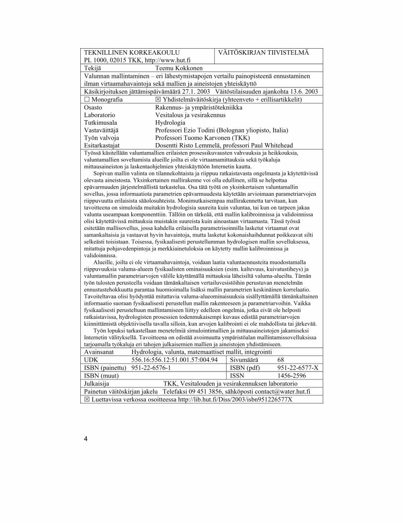
Tekijä Teemu Kokkonen Valunnan mallintaminen – eri lähestymistapojen vertailu painopisteenä ennustaminen ilman virtaamahavaintoja sekä mallien ja aineistojen yhteiskäyttö Käsikirjoituksen jättämispäivämäärä 27.1. 2003 Väitöstilaisuuden ajankohta 13.6. 2003

Monografia Yhdistelmäväitöskirja (yhteenveto + erillisartikkelit) Osasto Rakennus- ja ympäristötekniikka Laboratorio Vesitalous ja vesirakennus Tutkimusala Hydrologia Vastaväittäjä Professori Ezio Todini (Bolognan yliopisto, Italia) Työn valvoja Professori Tuomo Karvonen (TKK) Esitarkastajat Dosentti Risto Lemmelä, professori Paul Whitehead Työssä käsitellään valuntamallien erilaisten prosessikuvausten vahvuuksia ja heikkouksia, valuntamallien soveltamista alueille joilta ei ole virtaamamittauksia sekä työkaluja mittausaineiston ja laskentaohjelmien yhteiskäyttöön Internetin kautta.

Sopivan mallin valinta on tilannekohtaista ja riippuu ratkaistavasta ongelmasta ja käytettävissä olevasta aineistosta. Yksinkertainen mallirakenne voi olla edullinen, sillä se helpottaa epävarmuuden järjestelmällistä tarkastelua. Osa tätä työtä on yksinkertaisen valuntamallin sovellus, jossa informaatiota parametrien epävarmuudesta käytetään arvioimaan parametriarvojen riippuvuutta erilaisista sääolosuhteista. Monimutkaisempaa mallirakennetta tarvitaan, kun tavoitteena on simuloida muitakin hydrologisia suureita kuin valuntaa, tai kun on tarpeen jakaa valunta useampaan komponenttiin. Tällöin on tärkeää, että mallin kalibroinnissa ja validoinnissa olisi käytettävissä mittauksia muistakin suureista kuin ainoastaan virtaamasta. Tässä työssä esitetään mallisovellus, jossa kahdella erilaisella parametrisoinnilla lasketut virtaamat ovat samankaltaisia ja vastaavat hyvin havaintoja, mutta lasketut kokonaishaihdunnat poikkeavat silti selkeästi toisistaan. Toisessa, fysikaalisesti perustellumman hydrologisen mallin sovelluksessa, mitattuja pohjavedenpintoja ja merkkiainetuloksia on käytetty mallin kalibroinnissa ja validoinnissa.

Alueille, joilta ei ole virtaamahavaintoja, voidaan laatia valuntaennusteita muodostamalla riippuvuuksia valuma-alueen fysikaalisten ominaisuuksien (esim. kaltevuus, kuivatustiheys) ja valuntamallin parametriarvojen välille käyttämällä mittauksia läheisiltä valuma-alueilta. Tämän työn tulosten perusteella voidaan tämänkaltaisen vertailuvesistöihin perustuvan menetelmän ennustustehokkuutta parantaa huomioimalla lisäksi mallin parametrien keskinäinen korrelaatio. Tavoiteltavaa olisi hyödyntää mitattavia valuma-alueominaisuuksia sisällyttämällä tämänkaltainen informaatio suoraan fysikaalisesti perustellun mallin rakenteeseen ja parametriarvoihin. Vaikka fysikaalisesti perusteltuun mallintamiseen liittyy edelleen ongelmia, jotka eivät ole helposti ratkaistavissa, hydrologisten prosessien todenmukaisempi kuvaus edistää parametriarvojen kiinnittämistä objektiivisella tavalla silloin, kun arvojen kalibrointi ei ole mahdollista tai järkevää.

Työn lopuksi tarkastellaan menetelmiä simulointimallien ja mittausaineistojen jakamiseksi Internetin välityksellä. Tavoitteena on edistää avoimuutta ympäristöalan mallintamissovelluksissa tarjoamalla työkaluja eri tahojen julkaisemien mallien ja aineistojen yhdistämiseen. Avainsanat Hydrologia, valunta, matemaattiset mallit, integrointi UDK 556.16:556.12:51.001.57:004.94 Sivumäärä 68 ISBN (painettu) 951-22-6576-1 ISBN (pdf) 951-22-6577-X ISBN (muut) ISSN 1456-2596 Julkaisija TKK, Vesitalouden ja vesirakennuksen laboratorio Painetun väitöskirjan jakelu Telefaksi 09 451 3856, sähköposti contact@water.hut.fi

Luettavissa verkossa osoitteessa http://lib.hut.fi/Diss/2003/isbn951226577X

5

LIST OF APPENDED PAPERS

This thesis is based on the following Papers:

I: Kokkonen, T.S., Jakeman, A.J., 2001. A comparison of metric and conceptual approaches in rainfall-runoff modeling and its implications. Water Resources Research 37(9), 2345-2352.

II: Kokkonen, T., Koivusalo, H., Karvonen, T., 2001. A semi-distributed approach to rainfall-runoff modelling - a case study in a snow affected catchment. Environmental Modelling & Software 16, 481-493.

III: Kokkonen, T.S., Jakeman, A.J., Young, P.C., Koivusalo, H.J., 2003. Pedicting daily flows in ungauged catchments - model regionalization from catchment descriptors at the Coweeta Hydrologic Laboratory, North Carolina. Hydrological Processes (in print).

IV: Kokkonen, T.S., Jakeman, A.J., 2002. Structural effects of landscape and land use on streamflow response. In: Beck, M.B. (Ed.), Environmental Foresight and Models: A Manifesto. Elsevier, Amsterdam, pp. 303-321.

V: Kokkonen, T., Koivusalo, H., Karvonen, T., Croke, B., Jakeman, A., 2003. Exploring streamflow response to effective rainfall across event magnitude scale. Hydrological Processes (accepted).

VI: Koivusalo, H., Kokkonen, T., 2003. Modelling runoff generation in a forested catchment in southern Finland. Hydrological Processes 17, 313-328. VII: Kokkonen, T., Jolma, A., Koivusalo, H., 2003. Interfacing environmental simulation models and databases using XML. Environmental Modelling & Software 18, 463-471.

Papers I–VII, reprinted with permission, are copyright as follows: Paper I copyright © 2001 by American Geophysical Union; Paper II copyright © 2001, Paper IV copyright © 2002, and Paper VII copyright © 2003 by Elsevier Science; Paper III, Paper V, and Paper VI copyright © 2003 by John Wiley & Sons, Ltd.

6

Contribution of the author to Papers from I to VII is as follows: I: The author of this thesis is responsible for initiating and writing the paper. Prof. Jakeman has provided comments both during the analysis of the results and writing the paper. II: The author is responsible for deriving characteristic profiles from elevation data. Dr. Koivusalo has provided snow model results. Prof. Karvonen has provided comments both during the analysis of the results and writing the paper. Runoff model application, analysis of the results and writing the paper have been accomplished jointly between the author and Dr. Koivusalo. III: The author is responsible for the GIS analysis and all computations. Prof. Jakeman and Prof. Young have provided comments during the analysis of the results and writing of the paper. Dr. Koivusalo has assisted in writing the paper after reception of the review comments. IV: The author is mainly responsible for writing the paper. Prof. Jakeman has also participated in writing and commented author’s text. This paper is a book section and is based on previous work by the author, Prof. Jakeman, and Dr. Schreider. The author is responsible for additional computations conducted particularly for this book section. V: The author is responsible for initiating the paper. Computations and writing the paper have been accomplished jointly between the author and Dr. Koivusalo. Prof. Karvonen, Dr. Croke, and Prof. Jakeman have provided comments

VI: The author has participated in the analysis of the results and writing the paper. Dr. Koivusalo is responsible for all computations. VII: The author has initiated the paper and developed the sample application presented in the paper. Writing the paper has been accomplished jointly by all authors.

7

ACKNOWLEDGEMENTS

This thesis is a result of my studies at two inspiring universities. I have been privileged to work alternatively over a five-year period at the Helsinki University of Technology (HUT) and the Australian National University (ANU). I am greatly indebted to professor Tuomo Karvonen and professor Pertti Vakkilainen at the HUT, and professor Tony Jakeman at the ANU. Not only am I grateful for their insights into hydrology and environmental science, but also for their support and encouragement at difficult moments during completion of this thesis.

I am most thankful to docent Risto Lemmelä and professor Paul Whitehead for pre-examining my manuscript.

I want to acknowledge all staff members and students in the Laboratory of Water Resources, HUT. Particularly I am in debt to Dr. Harri Koivusalo, whose support and friendship have been invaluable.

I am most thankful to staff and students in the Centre for Resource and Environmental Studies (ANU), and to my wonderful housemates in Canberra, for always making me feel welcome during my visits in Oz.

This study was mainly funded from an Academy of Finland project “Predicting impacts of land use changes on catchment hydrological processes”. Other funding was received from the Land and Water Technology Foundation (Maa- ja vesitekniikan tuki ry.), the Finnish Cultural Foundation, the Jenny and Antti Wihuri Foundation, the Sven Hallin Foundation, and the Australian National University. All funding is greatly acknowledged.

Finally, I wish to thank my family for their support and interest into my studies. And for not asking too often, when this work would be completed.

Espoo, 21.5.2003 Teemu Kokkonen

8

TABLE OF CONTENTS

Abstract of doctoral dissertation ....................................................................................... 3 Väitöskirjan tiivistelmä ..................................................................................................... 4 List of appended papers .................................................................................................... 5 Acknowledgements........................................................................................................... 7 Table of contents............................................................................................................... 8 1 Introduction ............................................................................................................. 9

1.1 Background ............................................................................................... 9 1.2 Objectives of the present study ............................................................... 10

2 Rainfall-runoff modelling...................................................................................... 11 2.1 Rational method ...................................................................................... 11 2.2 Unit hydrograph ...................................................................................... 11 2.3 Conceptualisation of rainfall-runoff relationships................................... 12 2.4 Physics-based runoff modelling .............................................................. 13 2.5 How to deal with uncertainty?................................................................. 16 2.6 Why not let the data tell?......................................................................... 17 2.7 The ungauged case .................................................................................. 18 2.8 Tracing the origin and route of runoff..................................................... 21 2.9 Integration requires communication........................................................ 22

3 Sites and methods .................................................................................................. 24 3.1 Andrews Watershed 2 ............................................................................. 24 3.2 Coweeta Hydrologic Laboratory ............................................................. 25 3.3 Salmon Brook.......................................................................................... 26 3.4 Rudbäck .................................................................................................. 27 3.5 Vantaanjoki basin.................................................................................... 28 3.6 IHACRES hydrological model................................................................ 29 3.7 Characteristic profile hydrological model ............................................... 32 3.8 IUH – gamma distribution function ........................................................ 33 3.9 Data transfer ............................................................................................ 34

4 Results and discussion ........................................................................................... 35 4.1 How to select a modelling strategy?........................................................ 35 4.2 Modelling of ungauged catchments ........................................................ 47 4.3 Model integration .................................................................................... 49

5 Conclusions ........................................................................................................... 52 6 References ............................................................................................................. 55 Appendix 1 List of symbols........................................................................................ 64

9

1 INTRODUCTION

1.1 Background

Although already during the Hellenic Civilization correct perceptions of the hydrological cycle had been put forward (e.g. Theophrastus, 371/370 – 288/287 B.C.), it was not until the 17th century that it was shown in quantitative terms that precipitation alone would be sufficient to support the annual flow of rivers. Pioneering scientists advancing quantitative hydrology include the Frenchman Pierre Perrault (1608 – 1680), the Italian Edmé Mariotte (1620 – 1684), and the Briton Edmond Halley (1656 – 1742). Perrault showed in a catchment in the Seine basin that the annual rainfall was approximately six times greater than the annual flow in the river, thus indicating that precipitation indeed was capable of supporting the river flow. Mariotte did the same for a much bigger basin (the river Seine near Paris) and he also concluded that the annual rainfall was more than six times greater than the annual runoff. Halley’s measurements showed that the amount of water evaporated from the oceans was clearly sufficient to sustain the flows of rivers.

Measurement based evidence indicating that rainfall alone could sustain river flow laid basis for searching mathematical relationships between precipitation and streamflow. Mathematical problem formulation is convenient in that it provides a documentable and repeatable way for problem definition and analysis. It can also be relatively objective, assuming that the structure of the model is based on well proven, widely accepted hydrological and/or system analytical principles.

As simulation of rainfall-runoff relationships has been a prime focus of hydrological research for several decades, an abundance of mathematical models has been proposed to quantify transformation of precipitation into streamflow. Following Beck (1991), mathematical rainfall-runoff models can crudely be classified as metric, conceptual and physics-based. Metric models are strongly observation-oriented, and they are constructed with little or no consideration of the features and processes associated with the hydrological system. Conceptual models describe all of the component hydrological processes perceived to be of importance as simplified conceptualisations. This usually leads to a system of interconnected stores, which are recharged and depleted by appropriate component processes of the hydrological system. Finally, physics-based models attempt to mimic the hydrological behaviour of a catchment by using the concepts of classical continuum mechanics.

Even if the hydrological circulation of water could be accurately simulated in a study basin, it would be evident that problems associated with water resources could not be solved by hydrologists alone. Increasing collaboration between hydrologists, economists, ecologists, water users, and decision makers is vital on the track towards more sound policies in water resources management. Collaboration between different disciplines and interest groups calls for more efficient sharing of data sets and methods, which may exist but not be compatible with each other.

10

1.2 Objectives of the present study

Objectives of this thesis fall under three main topics. Firstly, this thesis aims at providing insight into selecting an adequate modelling strategy for a rainfall-runoff study (Section 4.1). Different strategies to model development are discussed and compared. Paper I compares metric and conceptual modelling approaches and discusses implications of increasing complexity in process description. A more physics-based approach is undertaken in Papers II and VI, which address, respectively, parameterisation of a semi-distributed model based on topographic data and simulation of other hydrological variables in addition to streamflow. Paper IV contributes to the objectives of the present thesis by presenting a case study where parametric uncertainty of a simple metric model is objectively quantified. In Paper V, following the metric modelling strategy, only little is assumed about the model structure a priori and data are used to infer whether differences in the hydrologic response can be detected and exploited in an improved model.

Secondly, this thesis seeks methods for predicting streamflow in ungauged catchments (Section 4.2). ‘Ungauged’ means here that flow records of sufficient length are not available to support calibration of model parameters against measured streamflow. Producing streamflow estimates for catchments lacking flow gauging has attracted a lot of interest among hydrologists, but the problem still remains somewhat unresolved. Opinions have been uttered (see e.g. Refsgaard, 1997) that a model should only be assumed to be valid with respect to outputs that have been explicitly validated. This is rather frustrating, if the objective is especially to model streamflow in areas where there are no streamflow measurements for either calibration or validation. Still, it is foreseeable that estimates of streamflow in ungauged catchments continue to be needed. In fact, many of the most acute problems concerning water quantity and quality are found in the third world countries, where long historical records are often not at hand. Paper III of the present thesis discusses a statistical approach to ungauged predictions. The objective is to study how well the hydrologic response of an ungauged catchment can be regionalised from other catchments belonging to the same region. Paper II addresses the ungauged problem from another perspective. It discusses how accurately streamflow can be reproduced when applying a more physics-based approach where most of the model parameters are fixed a priori and only little calibration is allowed.

Finally, as the third topic of the thesis, a methodology for integrating environmental simulation models and data sources is discussed (Section 4.3, Paper VII). It is not only lack of data which causes problems for an environmental modeller. Even if the data are available, they may be scattered among numerous sources and exist in heterogeneous formats. The same is true for simulation models. Agreement on techniques of how to transfer information between data sources and models is one of the key issues to be solved in integrated management of environmental problems. Model and data source integration is further motivated in the present thesis, as it itself is based on data sets from three continents and application of several simulation models.

2 RAINFALL-RUNOFF MODELLING

2.1 Rational method

Probably the first serious attempts to estimate flood flow volumes can be traced back to a group of Irish engineers, who were given the task to design drainage channels in 1842 (Biswas, 1970). Ten years later, in 1851, Thomas Mulvaney (1822 – 1892) presented a paper which can be considered as the origin of the so-called rational method for flood peak estimation (Dooge, 1957). The method can be written as

11

APf maxr=

− ττ dtr )()

qmax (1)

where qmax is the maximum rate of runoff, fr is the runoff coefficient, Pmax is the maximum rate of rainfall, and A is the area of the catchment. The rational method has stood the test of time well as a simple tool to estimate peak flows. The latest edition of the Handbook of Hydrology presents the rational method in the flood runoff chapter (Pilgrim and Cordery, 1992), and Pilgrim (1986) names it as the most widely used method for drainage design in urban areas.

2.2 Unit hydrograph

It took 80 years before significant progress over the rational method was achieved in representing rainfall-runoff relationships mathematically. It came with the method proposed by Sherman (1932) which allowed calculation of continuous hydrographs as opposed to merely delivering a peak flow estimate of the maximum flood event. Sherman called his method a unit-graph method, but it is presently better known as the unit hydrograph method. In essence, the unit hydrograph is equivalent to the systems analysis concept of the impulse response function, which depicts the response, x(t), of a system to an infinitesimally short unit input. The output of a linear system, resulting from a continuous input, i(t), is given by the following convolution integral

(2) ∫= τitx ()(

where r(t) is the impulse response function. In the case of rainfall-runoff computations, the input in Equation (2) is

rainfall multiplied by the (surface) runoff coefficient. This is because, mainly due to evapotransporative losses, not all of the rainfall is converted into streamflow. Furthermore, Sherman thought the output of Equation (2) to represent only the quick, surface runoff component. The so-called base flow, which is the part of a hydrograph preceding a storm and continuing after recession of a flow peak, he attributed to discharge of groundwater.

12

Since its proposal the unit hydrograph has established itself as a widely used engineering tool for assessing real floods, and for creating design floods from hypothetical storms. Pilgrim and Cordery (1992) describe the HEC-1 model (http://www.hec.usace.army.mil/publications/pubs_distrib/ hec-1/hec1.html) as the most widely used model in the United States, and it includes the unit hydrograph as one of the two available computation methods for runoff generation. Recent publications reporting application of the unit hydrograph include Cheng and Wang (2002) and Littlewood (2001). In Finnish conditions, Mustonen (1963) derived unit hydrographs separately for storm events of short and long duration using data from a small, cultivated catchment (0.12 km2).

The linearity assumption behind the unit hydrograph methods was later subject to criticism and it was suggested that the unit hydrograph itself, not only the share of rainfall becoming effective rainfall, might vary with the storm intensity (e.g. Minshall, 1960). Consequently, some papers have put forward unit hydrographs that depend on the intensity of the effective rainfall (Chen and Singh, 1986; Ding, 1974). Results presented in Section 4.1 of the present thesis clearly suggest that given any plausible series of effective rainfall, a single unit hydrograph may not be sufficient to adequately describe conversion of effective rainfall into streamflow in the two smallest catchments (0.18 and 0.63 km2) of the study.

2.3 Conceptualisation of rainfall-runoff relationships

Usually analysts have some kind of a perception in their mind about the behaviour of the hydrological system under study. The rationale for incorporating such concepts into the structure of a hydrological model can be an attempt to reproduce streamflow more accurately at the point of interest, or the need to include representations of various hydrological fluxes and runoff pathways into the model.

In 1934 Zoch (1934) developed equations relating rainfall to the rate of runoff, based on the assumption that the rate of runoff is proportional to the rainfall remaining with the soil. This is probably among the first published studies, where a linear store is applied to represent the delay between rainfall and streamflow. Later Nash (1957) showed how the response of a cascade of such linear stores could be characterised as a mathematical function involving two parameters. Nash’s primary motivation was to introduce a computationally convenient form for an instantaneous unit hydrograph in order to relate its parameters to catchment characteristics. But he also made the concept of linear stores as a delay mechanism in runoff computations popular1. This paved the way for the development of conceptual rainfall-runoff models, usually comprising interrelated stores recharged and depleted by appropriate component processes of the hydrological system.

One of the first conceptual, hydrological models for continuous streamflow simulation was that of Linsley and Crawford (1960), which was developed to assess increase of the capacity of one of the water-

1 The cascade of linear stores with equal time constants is often referred to as the Nash’s cascade, although he himself attributed the concept in the 1957 paper to Sugawara and Maruyama (1956).

supply reservoirs of the Stanford University. The structure of the model (Figure 1) is typical of many conceptual streamflow models, comprising storages representing upper level soil moisture, lower level soil moisture, groundwater, and water in the channel. The same group published later the well-known Stanford Watershed Model (Crawford and Linsley, 1966).

Increased computing power advanced development of conceptual models, and since the early efforts in the 1960’s a plethora of alternative structures for conceptual hydrological models have been suggested worldwide. Such models include the HBV model (Bergström and Forsman, 1973) in Sweden, the Sacramento model in the United States (Burnash et al., 1973), the TANK model (see e.g. Franchini and Pacciani, 1991) in Japan, the MODHYDROLOG model (Chiew and McMahon, 1994) in Australia, the XIANJIANG model (Zhao et al., 1980) in China, the ARNO model in Italy (Todini, 1996), and the SATT-I model in Finland (Vakkilainen and Karvonen, 1982).

RUNOFF FROM IMPERVIOUS AREA

TO AMFLOWSTRE

TO AMFLOWSTRE

TO AMFLOWSTRE

RUNOFF ABOVE INFILTRATION CAPACITY

DEPLETION

ACCRETION TO GROUNDWATER

PRECIPITATION

UPPER LEVELMOISTURE

CHANNELSTORAGE

GROUNDWATERSTORAGE

LOWER LEVELMOISTURE

EVAPORATIONTO ATMOSPHERE

"LOST"GROUNDWATER

MEANDAILY FLOW

DEPLETION

DEPLETION

LIMITED BY THE POTENTIAL EVAPOTRANSPIRATION

Figure 1. A flow diagram of the Linsley and Crawford model. Adopted from Linsley and Crawford (1960). For comparison, see schematic representation of the IHACRES model, which has been applied in the present thesis (Figure 9).

Conceptual rainfall-runoff models have found wide application in practical problems. As an example, the operational flood forecasting system in the United States is based on the Sacramento model (see e.g. Thiemann et al., 2001), and in Finland on the HBV model (Vehviläinen, 1992).

2.4 Physics-based runoff modelling

Advances in computing technology not only played a significant role in the development of conceptual hydrological models. They certainly also promoted emergence of distributed hydrological models. Distributed models – in contrast to lumped models which consider large entities (such as the entire catchment) – split the modelling domain into several units. It does not need to be so, but distributed hydrological models tend to have a

13

14

clearly formulated physical basis underlying their process descriptions, and hence they often fall into the category of physics-based models.

At the end of the 1960’s Freeze and Harlan (1969) proposed a blueprint for a ‘physically-based hydrologic response model’. They envisaged a model which combines physics-based descriptions of various hydrological subsystems and whose parameters are spatially distributed over the modelling domain. Two years later Freeze (1971) presented a model structure, which probably can be considered as the first realisation of the above-described blueprint. He proposed a three-dimensional, saturated-unsaturated flow model and explored development of pressure head distributions under different hypothetical scenarios with a particular focus on the yield of a groundwater basin subject to water extraction. Later he extended the model to include a simple one-dimensional channel flow scheme, which was fed by the subsurface model described in the 1971 paper (Freeze, 1972a; Freeze, 1972b). Freeze’s pioneering work attracted many followers. Well-documented physics-based, distributed hydrological models include the SHE model (Abbott et al., 1986) developed as a joint European effort, the IHDM model (Rogers et al., 1985) in the United Kingdom, the DHSVM in the United States (Wigmosta et al., 1994), the model of Kuchment et al. (2000) in Russia, and the THALES model (Grayson et al., 1992a) in Australia.

In the Freeze and Harlan (1969) blueprint, output of the envisaged model is seen to provide ‘a total picture of the hydrologic system’ including ‘the streamflow hydrograph at any point within the basin, the groundwater flow pattern and the soil moisture regime’. As the motivation to pursue the physics-based, distributed modelling strategy the authors suggest that a better understanding of the internal processes could be beneficial to the solution of practical problems. After thirty years of distributed hydrological modelling the motivation remains the same. Assessment of problems dealing with water quality, erosion, and human impact on catchment response (such as drainage, irrigation, forest management, and urban development) places high demands on the quantitative hydrologist. Simulation models should consider spatial distribution of dominant processes, be capable of separating between various water transport mechanisms, and allow predictions to be made to catchments lacking historical records used for parameter calibration.

But even today, satisfactory physics-based modelling descriptions of hydrological processes continue to evade hydrologists. Soon after publication of the first distributed hydrological model (see above Freeze, 1971; Freeze, 1972a; Freeze, 1972b) it was realised that although such models can provide detailed hydrologic predictions within the catchment, it is very doubtful whether the simulated values adequately represent the ‘true’ behaviour of the catchment. When Stephenson and Freeze (1974) applied the Freeze (1971) model to field data measured in a small upstream source area in Idaho, the United States, they encountered considerable difficulties in finding an agreement between measured and computed hydrologic variables without actually calibrating model parameters. In most (if not all) subsequent comparisons between observed data and simulation results of a physics-based runoff model, parameter values have been calibrated. Although physical parameter values in

15

principle are physically measurable in the field, calibration seems to be nearly always necessary.

Probably the most often heard argument against soundness of mathematical formulations depicting hydrological processes is related to the discrepancy between the measurement and computation scales (see e.g. Beven, 1989; Beven, 1996; Grayson et al., 1992b; Jensen and Mantoglou, 1992). When physical model parameters applicable in some smaller scale are averaged over the grid scale, they are commonly referred to as effective parameters. It can be argued that such effective parameters, which lump the effect of several small-scale processes into (a much larger) grid scale, are actually equivalent to parameters of lumped, conceptual models (see e.g. Beven, 1989; Beven, 1996). They cannot be directly measured in the field. One suggested avenue for bridging the gap between measurement and computation scales is to simplify the model structure in such a manner that it would be compatible with the scale where the effect of local heterogeneities inherent in the natural system becomes attenuated (Grayson et al., 1992b). Beven (1996) speculates that if it were possible to measure directly the volume of water stored in a block or hillslope of soil, then hydrological theories might be developed at that scale.

Problems arising from the difficulties to measure hydrologically relevant catchment characteristics at appropriate scales need to be overcome before physics-based runoff modelling can proceed much further. In a recent paper by Beven (2001), it is stated that the characteristics for subsurface flow processes are essentially unknowable with present measurement methods. Remote sensing techniques have been seen as a promising avenue for data acquisition for distributed hydrological models. However, Kite and Pietroniro (1996), in their comprehensive review of the use of remotely sensed data in hydrological modelling, note that ‘there are few case studies that show practical benefits’. The difficulty in using remote sensing information is that it does not provide direct estimates of hydrological variables or parameters, but an interpretative model is required, which itself is subject to uncertainties (Andersen et al., 2002; Beven, 2001).

Computational burden in distributed runoff models is now less problematic than earlier, although it still can be an issue when predictive uncertainty of a model is assessed through laborious Monte Carlo simulations (see Beven, 2001; Beven, 1996). Computational demands, however, along with the difficulties of measuring hydrological variables and parameters in the field, motivated introduction of the semi-distributed modelling schemes. Probably the most-cited such model is that of Beven and Kirkby (1979), which utilises distributed observations on the catchment topography to estimate the extent of contributing (i.e. saturated) areas. The model was later called, owing to the importance of the topographic control in the model structure, the TOPMODEL and it has received a substantial amount of attention in the form of model applications (Durand et al., 1992; Holko and Lepistö, 1997), proposals for alternative formulations (Ambroise et al., 1996), and critical assessments of the model structure and model sensitivity (Franchini et al., 1996; Wolock and Price, 1994). Another common approach to simplify the spatial description of the study region is to identify areas which are assumed to possess similar hydrological behaviour, and then lump such

16

areas together to form a single computation unit (Becker and Braun, 1999; Flügel, 1995; Karvonen et al., 1999; Schultz, 1993).

To conclude the discussion on distributed, physics-based hydrological modelling, it is noted that the future of such modelling efforts can be much brighter than what could be interpreted from the critics presented above. Firstly, and most importantly, there is a strong consensus that distributed predictions on hydrological variables within a catchment are required. This is almost without exception expressed in all studies dealing with distributed hydrological modelling, irrespective of whether the authors are promoting or criticising current modelling practices. Such a collective demand is likely to continue to generate efforts that aim at furthering understanding of how to represent a catchment’s hydrological behaviour in a distributed setting. An easier access to distributed data, owing to both remote sensing techniques and more organised acquisition and storage of point data, encourages a wider application of models capable of handling spatial variability. For example, Andersen et al. (2002) and Biftu and Gan (2001) report on recent studies where remotely sensed data have been applied in hydrological modelling with some success. Distributed, physics-based rainfall-runoff modelling is a controversial topic, which is prone to invoke discussion and split opinions. This can be seen from several response articles to critical assessments of physics-based hydrological modelling (Loague, 1990; Refsgaard et al., 1996; Smith et al., 1994). As argued by Refsgaard (1997), distributed models may still be the best tools presently available for certain tasks, such as assessing the effects of land use changes on a catchment’s hydrological behaviour. Efforts for narrowing the gap between what hydrologists want to do and what they can do will continue.

2.5 How to deal with uncertainty?

The increase in computing power did not only allow for more complicated model structures to be fabricated; it also enabled automatic optimisation methods to be applied to estimation of parameter values. Soon it was realised that obtaining a unique, ‘true’ set of parameter values for a rainfall-runoff model is not a trivial exercise, even though computing power would not be a limiting factor.

In the often-cited paper by Johnston and Pilgrim (1976) the authors concluded that, in spite of more than two years of full-time work concentrating on one catchment, a true optimum set of model parameter values could not be identified. It is not surprising that Johnston and Pilgrim (1976), who used real field data, failed in obtaining a unique set of model parameter values. A little later Pickup (1977) studied basically the same model with synthetic data, and even under such idealised conditions the true set of parameters used for generation of the flow record could not be recovered. It is intuitively conceivable, and has also been demonstrated in previous studies (see e.g. Kuczera and Williams, 1992; Sorooshian and Gupta, 1983), that data errors arising from uncertain measurements, and inadequacies in the model structure can lead to troublesome parameter identifiability. Furthermore, in synthetic studies it is easier to assure sufficient variability of the hydro-meteorological data. Variability of the

17

data enhances identifiability by activating different model parameters responsible for representing different catchment conditions (Gan et al., 1997; Sorooshian et al., 1983). Sorooshian and Gupta (1983) state in their conclusions that ‘most conceptual R-R [short for rainfall-runoff] models cannot be properly identified even when ‘perfect’ (synthetic) data is used. The presence of errors in the model makes the identification problem even more difficult’.

Statistical methods have appeal in uncertainty analysis as they implicitly take into account that all model structures are, to some extent, in error and all measured data are also subject to error. Mein and Brown (1978) published one of the early studies to address parameter identifiability in rainfall-runoff models in a statistical setting. They derived a covariance matrix for the fitted parameter vector of a conceptual rainfall-runoff model. Kuczera (1983a) used Bayesian methodology and data from a small (0.623 km2) experimental catchment to derive posterior distributions for a nine-parameter catchment model. In Kuczera (1983b) the Bayesian methodology was applied to address how measurements on variables other than streamflow (interception and soil moisture observations were considered) can be utilised to reduce parameter uncertainty. Beven and Binley (1992) also base their Generalized Likelihood Uncertainty Estimation (GLUE) (see also Freer et al., 1996) on Bayesian reasoning. Thiemann et al. (2001) present a Bayesian methodology for recursive parameter estimation in rainfall-runoff models.

Dealing with uncertainty in hydrological modelling is not straightforward. It can be computationally demanding, and the amount of data may appear to be too small to justify statistical assessments. When the latter is the case, a question worth asking is whether there are enough data to produce credible simulation results. Considering that models are quite imperfect representations of the real hydrological processes, it is important to address the problem of uncertainty. Only then can decision makers evaluate how much weight can be placed on the simulation results for management of water resources.

However, if all hydrologists, owing to their insight into the level of uncertainty, decided to abstain from giving an opinion in water resources planning problems, then others, who are less knowledgeable in hydrology, would have to venture a guess.

2.6 Why not let the data tell?

The concept of the unit hydrograph is an empirical one (see Section 2.2). It relies on the data and does not really consider what the physical processes involved in runoff generation are. Such metric models tend to have a simple structure and their data and computational requirements are usually less than for other types of hydrological models. Furthermore, due to the simple structure, it is in general easier to derive statistical measures of uncertainty for metric models than for more complex conceptual or physics-based models. In fact, the discharge response to rainfall is relatively simple to model at the catchment scale; following a rainfall, the stream discharge rises and then falls again with a certain characteristic timing (Beven, 1996). Jakeman and Hornberger (1993) and Perrin et al.

18

(2001) both conclude that complexity of a (lumped) rainfall-runoff model could be restricted to a structure involving only a handful of parameters.

According to some hydrologists, it does not need to be that simple models developed by rigorous statistical analysis could not be related to the real phenomena. Young (2001; 2002) discusses a modelling philosophy called ‘data-based mechanistic modelling’, where statistical tools are first applied to identify the most parametrically efficient model structure, and following this initial identification stage the resulting model is interpreted in a physically meaningful, mechanistic manner. Young (2002) states that the model is only accepted as a credible representation of the system if ‘in addition to explaining the data well, it also provides a description that has direct relevance to the physical reality of the system under study’. Here the reasoning underlying conceptual models is essentially turned around. Instead of imposing a priori a structure on the model, and then trying to fit that structure to the observed data, the model structure is interpreted only after analysis of the data. Jakeman et al. (1994) express similar ideas in their ‘data and theory to model’ approach where the modelling process is started with simple assumptions and additional complexity in the model structure is accepted only when observed data and theory warrant it.

Whichever modelling strategy is selected for representing rainfall-runoff relationships, measured data will have a vital role in determining how successful the modelling exercise is likely to be. It is now increasingly accepted that more emphasis needs to be placed on gathering field data in order to achieve improvements in environmental modelling (see e.g. Beven, 2002; Goodrich and Woolhiser, 1991; Vertessy et al., 1993). Pioneering efforts in collection of hydrological data include the following two contributions. Firstly, the United States Geological Survey and its antecedent organisations initiated systematic collection and publication of streamflow data for representative streams across the nation towards the latter half of the nineteenth century (Biswas, 1970). And secondly, in the 1930’s the Finnish National Board of Agriculture arranged a network of representative catchments extending across the nation (Kaitera, 1936) where, in addition to streamflow, precipitation and snow water equivalent were also observed. The catchments were mapped and information describing topography, vegetation, and soils was recorded.

2.7 The ungauged case

The preceding section concluded with highlighting the value of data in rainfall-runoff studies. However, a studied catchment may not have historical runoff records due to lack of flow gauging, or the catchment of interest may be subject to proposed changes in land use practices, and the aim of the study may be to assess hydrological impacts of such practices. In the first case the catchment is literally ungauged for flow, whereas in the latter case it is ungauged in the sense that the existing flow records are not representative of the changed conditions. This section explores existing methods to deal with situations when little or no streamflow data are available from the site of interest to support model calibration.

19

The problem of predicting streamflow in ungauged areas is not new. Already Sherman (Sherman, 1932; see Section 2.2) noted in his paper that ‘when no streamflow records from a particular area are available, it is possible to determine a unit graph by analogy from unit graphs from similar basins with like topographical characteristics’. Snyder (1938) proposed a quantitative relationship between the two parameters of his function for a unit hydrograph and catchment characteristics. Nash’s (1957) motivation to describe the unit hydrograph with a function involving just two parameters was the desire to link those parameters to catchment characteristics (see Section 2.3). Assuming that the identified relationships between runoff model parameters and catchment descriptors hold for the catchment lacking flow gauging, runoff simulations can be carried out for the ungauged catchments by estimating model parameters from the physical catchment descriptors (topography, soil depths, flow network geometry etc.). This type of methodology where information is transferred from one or more catchments to another is commonly called regionalisation (e.g. Blöschl and Sivapalan, 1995), and has been widely used in runoff modelling (see the review in Bates, 1994). Bates (1994) lists five critical topics on which successful regionalisation of rainfall-runoff model parameters depends. These are 1) accurate estimation of model parameters for gauged catchments, 2) selection of catchment descriptors that affect catchment response to rainfall, 3) delineation of homogenous regions, 4) degree to which the model parameters are correlated with catchment characteristics, and 5) correct specification of the regression model for each region. Topic 1) was addressed in Section 2.5, and topics 2), 4), and 5) are self-explanatory. Delineation of homogenous regions, topic 3), warrants further discussion.

To have a greater confidence in extrapolating hydrological behaviour from catchments with flow records to an ungauged catchment, all these catchments should form a relatively homogeneous group (Nathan and McMahon, 1990; Pilgrim, 1983; Post and Jakeman, 1996). The simplest method to delineate hydrologically homogeneous regions is merely to consider geographical proximity. Such a grouping is easy to perform but, as argued by Wiltshire (1986), geographical proximity may not be a very useful indicator of hydrological similarity. Statistical techniques such as cluster analysis have also been applied to identify hydrological homogeneity using data on climatological and/or terrain attributes (Acreman and Sinclair, 1986; Burn and Boorman, 1993; Tasker, 1982). The need first to group catchments according to hydrological similarity indicates that regionalisation is a technique for interpolating catchment response within a group of catchments possessing a relatively similar behaviour. Potter (1987) noted, in the context of predicting flood quantiles, that the greatest challenge in applying regionalisation techniques is defining homogeneous regions.

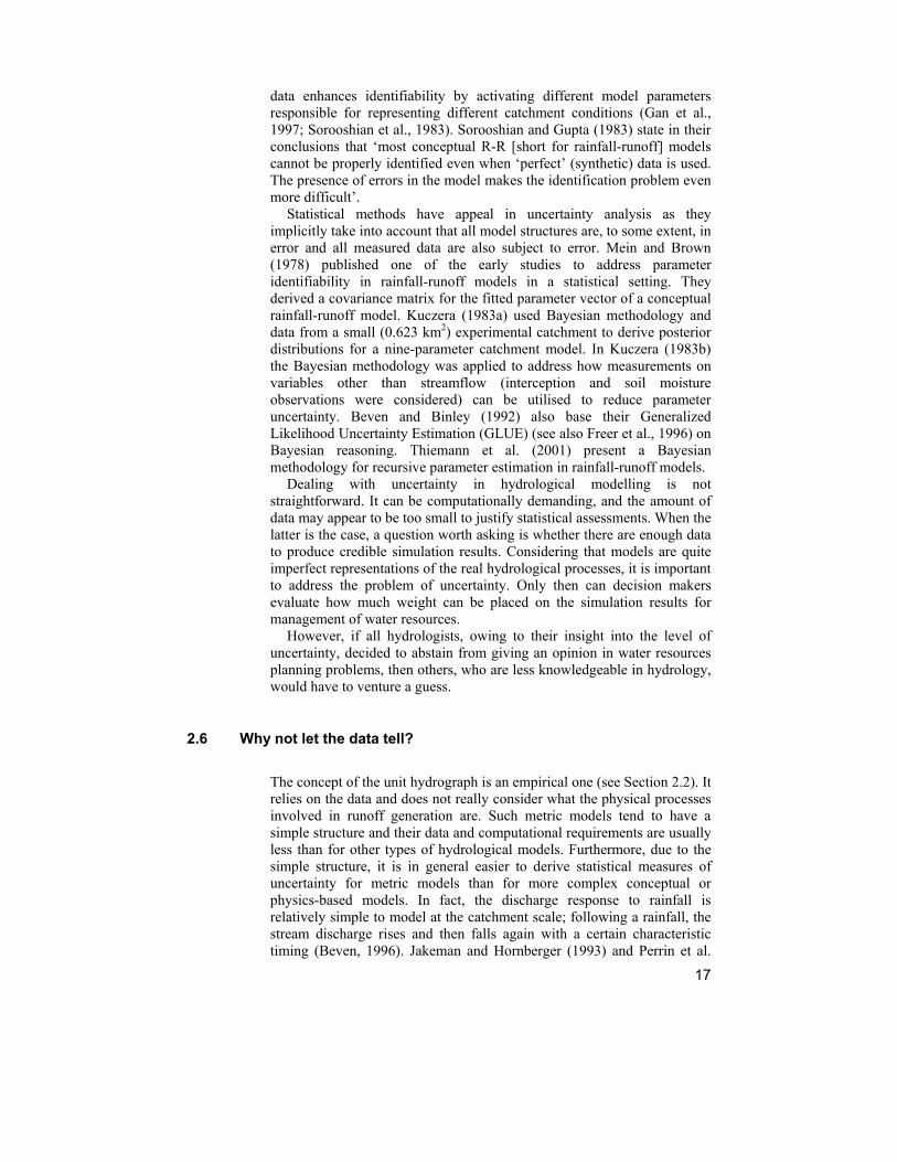
It is far from straightforward to be confident that all dominant controls on the catchment behaviour have been included into a regionalisation analysis. The paper by Post and Croke (2002) provides an illustrative example of this (see Figure 2). Three different relationships linking summer precipitation to percent yield (share of rainfall becoming streamflow) were developed for three groups of catchments. In particular the catchments in the Bowen region behave in a very different way

compared to the other two groups, and the reason for this difference is unknown (Post and Croke, 2002). Now if the catchments in the Bowen region were ungauged, and the percent yield in those catchments was to be predicted using information from the other catchments in Figure 2, regionalisation would yield erroneous results.

Often in regionalisation studies the predictive focus has been on a certain flow regime. In particular, estimation of flood indices for ungauged catchments has received a great deal of attention (e.g. Farquharson et al., 1992; Mimikou and Gordios, 1989; Zrinji and Burn, 1994). Nathan and McMahon (1990) considered low flow characteristics, which may be of importance with respect to the ecological health of a river system. Hyvärinen (1984) presented correlations between concurrently occurring summer and winter flows in a set of Finnish catchments. More recently, studies aimed at simulating continuous flow records have started to emerge. Vandewiele and Elias (1995) reconstruct monthly runoffs for basins considered to be ungauged; while Post and Jakeman (1999), Sefton and Howarth (1998), and Wheater et al. (2002) predict daily flow time series by developing relationships between the parameters of a daily time step rainfall-runoff model and physical catchment descriptors.

0

5

10

15

20

25

30

0 50 100 150 200 250 300

Summer precipitation (mm)

% Y

ield

Upper Burdekin

BowenBeylandoSuttor

350 400

Summer precipit at ion [mm]

Yiel

d [%

]

Figure 2. Predicting percent yield from summer precipitation in three groups of catchments. Adopted from Post and Croke (2002).

Physics-based rainfall-runoff models should have physically meaningful, measurable parameter values, and hence they should be capable of simulating streamflow in ungauged catchments lacking historical flow records required for parameter calibration. The difficulties of the current generation physics-based models were discussed at length in Section 2.4, and are not repeated here. The geomorphologic instantaneous unit hydrograph (GIUH) of Rodríguez-Iturbe and Valdés (1979) links the basin response to (measurable) geomorphologic parameters, and can hence be interpreted as a physics-based method of predicting flows for ungauged catchments. However, the methodology presented in Rodríguez-Iturbe and Valdés (1979) attempts to describe the streamflow response to surface

20

runoff, not directly to precipitation and other meteorological variables, and is not alone applicable to ungauged predictions2.

2.8 Tracing the origin and route of runoff

Often it may be sufficient to simulate the volume of streamflow at a certain location with no consideration of the travel path or origin of water appearing in the stream. Increasingly, however, hydrologists are faced with questions where explicit knowledge of the sources, residence times, and travel routes of water that eventually emerges in the stream is essential. Problems related with water quality, such as leaching of nutrients and contaminants from cultivated land, require consideration of physical, chemical, and biological processes, which are dependent on transport routes and flow residence times. A better understanding of flow pathways is one of the key advances required in tackling catchment-scale water management issues in a more general setting where merely predicting water quantities is not enough. Kendall et al. (1995) states that, of all the methods to understand hydrological behaviour in small catchments, tracer studies have been most useful in shedding light on the hydrological processes because they integrate small-scale variability and give an effective indication of catchment-scale processes.

Isotopes of oxygen and hydrogen forming water molecules are commonly used as tracers of water sources. The two main processes governing oxygen and hydrogen isotopic concentrations of waters within a catchment are 1) phase changes, and 2) mixing of waters having a different isotopic composition (Kendall et al., 1995). The following simple mixing model is typically used to identify contributions of stream water from two distinct sources:

21

s2s2s1

s2

QC+

(3) s1ss

s1s

QCQCQQQ

=+=

where Qs is the total stream discharge, Qs1 is the source one contribution to the total discharge, Qs2 is the source two contribution to the total discharge, Cs is the tracer concentration in stream water, Cs1 is the tracer concentration in source one, and Cs2 is the tracer concentration in source two.

Hydrograph separation has been undertaken for a long time. As discussed in Section 2.2, unit hydrograph based methods normally involve a separation of the total hydrograph into baseflow and quick component of runoff. Traditionally the quick component has been associated with surface runoff, and baseflow with discharge of groundwater into the stream. The latter concept is intuitively very conceivable, as at times of no precipitation (or snowmelt) the flow of stream must be sustained by waters stored in the ground. The origin of the fast responding runoff component,

2 It is worth noting that the authors do not promote the GIUH as a tool for ungauged predictions, but rather as a means to understand ‘the nature and development of existing hydrologic hierarchies’.

22

however, is much more open to debate. According to isotope and chemical hydrograph studies it appears that most stormflow in humid temperate environments is ‘old water’ (Kendall et al., 1995 ref . Bishop, 1991). Kendall (1995) defines old water as the water that existed in a catchment prior to a particular storm or snowmelt period; hence the quick responding part of streamflow would not then originate from the precipitation (or snowmelt) triggering the flow event. Sklash and Farvolden (1979) found groundwater to be a major component (sometimes more than 80% in peak discharge) virtually in all of the runoff events that they documented in their study. Results of Rodhe (1987) contribute between 32% and 95% of the streamflow to groundwater. Lepistö et al. (1994) studied the relationships between event water fraction and event rainfall in Siuntio and found that the new water fraction becomes dominant only in response to intense storms.

Although isotope tracing can provide valuable insights into sources of water found in streams, it cannot directly determine what the runoff generating mechanisms are and how the water reaches the stream (Kendall et al., 1995). Some information about flowpaths can be inferred when reactive solute isotopes are used in the tracer studies, as they can reflect the reactions that are characteristic of certain flow routes (Bullen and Kendall, 1991). As noted by Robson et al. (1992), the need to incorporate flowpath dynamics is a key ingredient in producing reliable water quality models. Traditional methods, using only streamflow data for hydrograph separation, can only differentiate between quick and slow response of streamflow. In order to obtain information about sources, residence times, and flowpaths of water in a catchment, additional data are required. Such data can consist of observations on internal hydrological variables (groundwater levels, soil moisture), or tracer measurements. Uhlenbrook and Leibundgut (2002) present a tracer-aided catchment model, where tracer investigations have been used to gain insights into runoff generation processes, and to validate modelling results.(Bishop, 1991)

2.9 Integration requires communication

This section addresses linking of various resources, which can be data sets or analysis tools. Such resources can include hydrological data and rainfall-runoff models, but also resources from other disciplines can be required. As pointed out in Section 1.1, integrated environmental analyses involving several disciplines and interest groups will increase in importance. An essential aspect of integration is the methodology which provides for communication between various parties. Without communication there is no integration.

Difficulty in linking data sets and analysis tools is one of the barriers to be overcome in developing integrated water resources management techniques (e.g. Huang and Xia, 2001). Development of modelling tools and acquisition of data sets often deal with relatively specific problems and this leads to troublesome model and data transferability. Parker et al. (2002) summarise deliberations of forty-five scientists dealing with integrated assessment and modelling in environmental problems, and they identified communication to be the critical factor in the success or failure

23

of integrated studies. Clearly, agreement on techniques of how to transfer information between data sources and models is one of the key issues in the integrated management of complex environmental problems.

Integration of simulation models has been implemented in many environmental assessment studies (e.g. Aspinall and Pearson, 2000; Booty et al., 2001; Huang et al., 1999). Computation frameworks particularly designed for handling different models – with minimal effort required for the integration – are sometimes called open modelling engines (Reed et al., 1999) or open modelling systems (Blind et al., 2001; Cate et al., 1998). Communication between model and data resources and the model user is crucial in the concept of the open modelling framework. The Internet – being an efficient means of communication – provides an attractive platform also in environmental studies to link models and data sets with each other. Section 4.3 presents results from a study where environmental models are coupled to a data source via the Internet.

3 SITES AND METHODS

First part of this section (subsections 3.1-3.5) briefly presents the sites whose data were used in this thesis. The remaining subsections give an outline to hydrological models (3.6-3.7) and data transfer techniques (3.8) included in the present thesis. For each site and method it is indicated in which Paper(s) I-VII it appears. Figure 3 depicts locations of the sites.

RVant

MAP:

udbäckaanjoki 700 mmCoweeta

MAP: 1870 - 2500 mm

Andrews WS2MAP: 2300 - 3550 mm

Salmon BrookMAP: 1200 mm

a)

b)

Figure 3. Location of Andrews WS2, Coweeta Hydrologic Laboratory, Rudbäck, and Vantaanjoki (a), and location of Salmon Brook (b). Indicative values of the mean annual rainfall (MAP) also shown.

3.1 Andrews Watershed 2

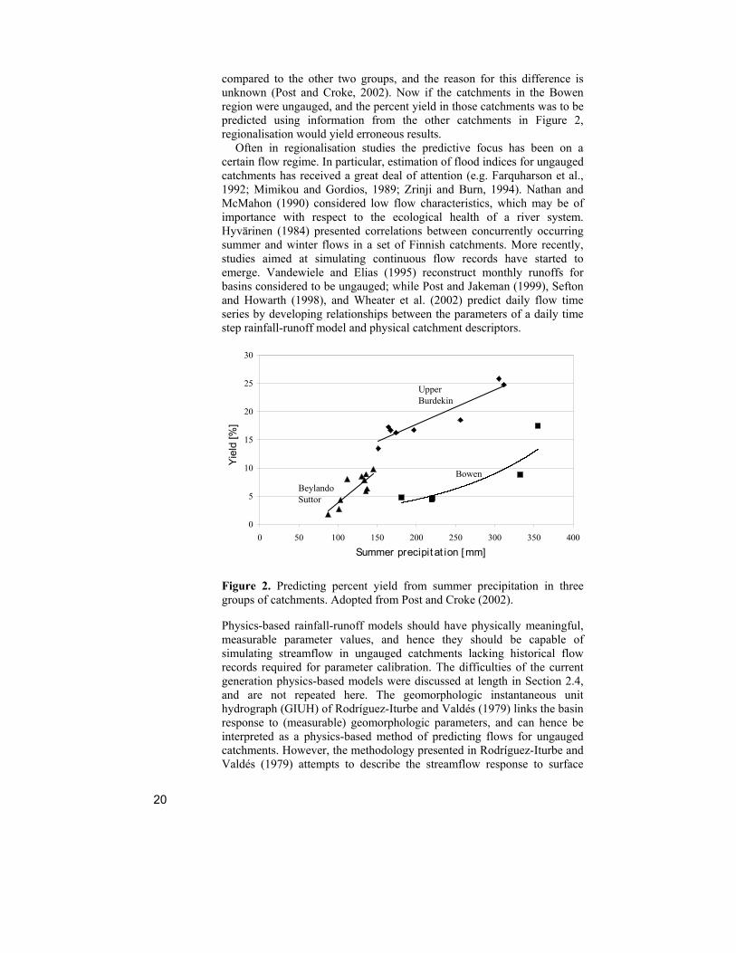
Andrews Watershed 2 (0.63 km2) is one of the research catcments in the H. J. Andrews Experimental Forest, Oregon, USA. Watershed 2 (Figure 4)

24

is completely forested with Douglas-fir and western hemlock as the dominating tree species. Elevation within the catchment ranges from 548 metres to 1070 metres and soils are predominantly composed of loams and clay loams.

The climate is maritime with wet, mild winters and dry, cool summers. The mean monthly temperature ranges from 1 ºC in January to 18 ºC in July. Average annual precipitation varies with elevation from about 2300 mm at the base to over 3550 mm at upper elevations, falling mainly in November through March. Rain predominates at low elevations; snowfall is more common at higher elevations. Highest streamflow occurs generally in November through February during rain-on-snow events.

The Andrews Watershed 2 data have been used in Paper V, where more detailed site information can also be found.

Figure 4. Watershed 2 in Andrews Experimental Forest, Oregon, USA.

3.2 Coweeta Hydrologic Laboratory

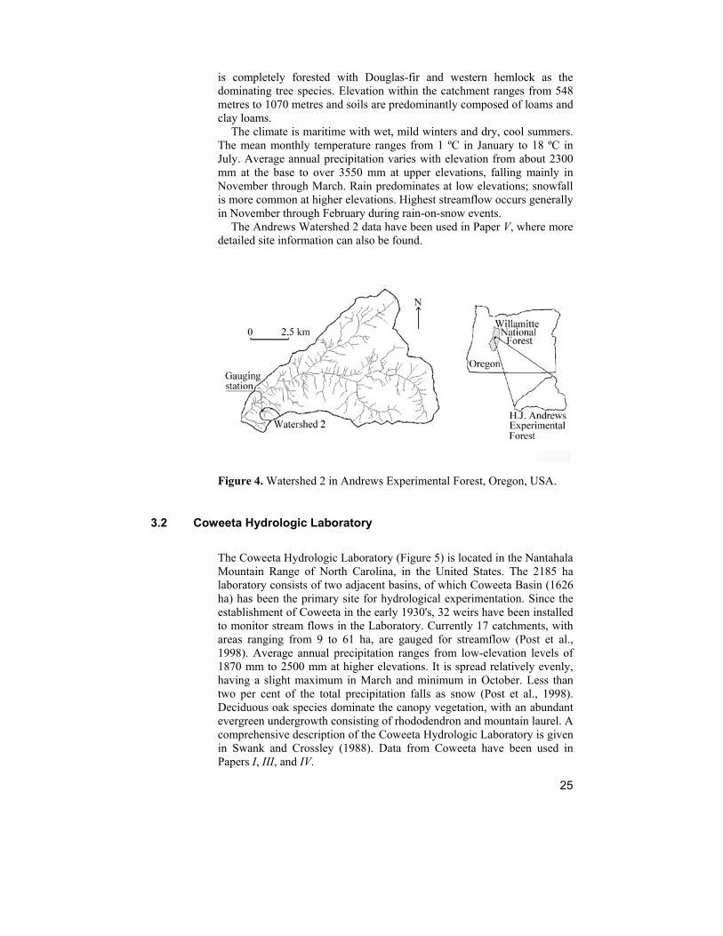
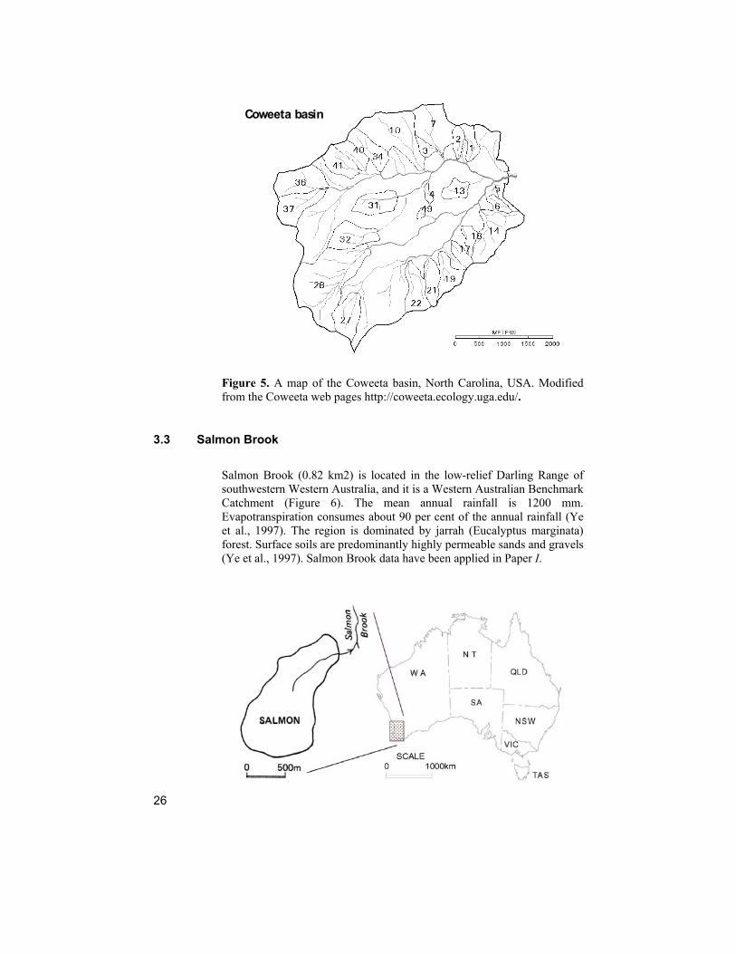
The Coweeta Hydrologic Laboratory (Figure 5) is located in the Nantahala Mountain Range of North Carolina, in the United States. The 2185 ha laboratory consists of two adjacent basins, of which Coweeta Basin (1626 ha) has been the primary site for hydrological experimentation. Since the establishment of Coweeta in the early 1930's, 32 weirs have been installed to monitor stream flows in the Laboratory. Currently 17 catchments, with areas ranging from 9 to 61 ha, are gauged for streamflow (Post et al., 1998). Average annual precipitation ranges from low-elevation levels of 1870 mm to 2500 mm at higher elevations. It is spread relatively evenly, having a slight maximum in March and minimum in October. Less than two per cent of the total precipitation falls as snow (Post et al., 1998). Deciduous oak species dominate the canopy vegetation, with an abundant evergreen undergrowth consisting of rhododendron and mountain laurel. A comprehensive description of the Coweeta Hydrologic Laboratory is given in Swank and Crossley (1988). Data from Coweeta have been used in Papers I, III, and IV.

25

Coweeta basin

Figure 5. A map of the Coweeta basin, North Carolina, USA. Modified from the Coweeta web pages http://coweeta.ecology.uga.edu/.

3.3 Salmon Brook

Salmon Brook (0.82 km2) is located in the low-relief Darling Range of southwestern Western Australia, and it is a Western Australian Benchmark Catchment (Figure 6). The mean annual rainfall is 1200 mm. Evapotranspiration consumes about 90 per cent of the annual rainfall (Ye et al., 1997). The region is dominated by jarrah (Eucalyptus marginata) forest. Surface soils are predominantly highly permeable sands and gravels (Ye et al., 1997). Salmon Brook data have been applied in Paper I.

26

27

Figure 6. Salmon Brook catchment in Western Australia. Modified from figures provided by Richard Silberstein (CSIRO Land and Water, WA, Australia) and Department of Environment, Water and Catchment Protection (Australia).

3.4 Rudbäck

Half-hourly streamflow and meteorological data were available from a small research catchment of the Finnish Environment Institute located in Siuntio, southern Finland (Rudbäck, 0.18 km2). The catchment (Figure 7) is covered by a mature forest stand dominated by Norway spruce. Elevation ranges from 34 to 65 metres above mean sea level. Bedrock is exposed on the hilltops and soils are composed of silty and sandy moraines with an average depth of 1 to 2 metres to the bedrock. More details on the site are published in Lepistö (1994) and Lepistö and Kivinen (1997).

The climate in Siuntio is temperate with cold, wet winters and precipitation is typically of relatively low intensity. Approximately 30 per cent of precipitation falls as snow. Mean annual precipitation, uncorrected for wind effects, was 700 mm during 1991-96. Mean monthly temperatures in February and July are –2 ºC and 16 ºC, respectively.

In 1996 a measurement campaign was initiated to provide meteorological, snow and streamflow data for calibration and validation of hydrological models (Koivusalo and Kokkonen, 2002; Koivusalo and Kokkonen, 2003; Koivusalo et al., 1999). The data from 1996 to 2001 include hourly records of precipitation, air temperature, relative humidity, wind speed, downward and reflected short-wave radiation, and long-wave radiation from an open site next to the catchment. Catchment data include hourly streamflow, and weekly measurements of snow depth and snow water equivalent, depth to the groundwater table, and throughfall beneath the canopy. Rudbäck data have been used in Papers II, V, and VI.

Figure 7. Rudbäck catchment in Siuntio, southern Finland.

3.5 Vantaanjoki basin

The Finnish Environment Institute provided daily streamflow records from two sub-catchments of the Vantaanjoki basin (Figure 8), a 58 km2 catchment gauged at Santamäki and a 1235 km2 catchment gauged at Myllymäki. The streamflow data covered the periods from 1971 to 1995 and from 1961 to 2001 for Santamäki and Myllymäki, respectively. Landuse in the Vantaanjoki basin comprises forest (46 %), agricultural land (29 %), urban areas (12 %), peat land (9 %), and open water bodies (3.5 %). Urban areas are concentrated in the south and the fraction of forest covered area increases towards the north. Forests are mainly scattered in the landscape as isolated patches. The elevation within the basin ranges from sea level up to 135 metres. Santamäki station is located at an elevation of 43 metres and Myllymäki station is just above sea level. The Salpausselkä ridge runs from south-east to north-west and divides the basin into two regions. Large depositions of sand and gravel are found in the ridge area. Sand and moraine soils predominate north of the ridge, and fine-grained materials are dominant south of the ridge. The climate south of the Salpausselkä ridge is similar to that of Siuntio, and north of the ridge it has a slightly more continental character. HWED (1994) provides a more detailed discussion on the Vantaanjoki area.

Precipitation and air temperature data were taken from meteorological stations operated by the Finnish Meteorological Institute (Figure 8). For Santamäki catchment the data were from Nurmijärvi, which is located 14 kilometres from the gauging station. Areal values of precipitation and air temperature for the Myllymäki catchment were computed with the Thiessen method (e.g. Smith, 1992) using point data from four stations (Helsinki-Vantaa airport, Nurmijärvi, Tuusula, Hyvinkää) located within the catchment. Areal estimates of the snow water equivalent were based on

28

snow course measurements from Tuusulanjärvi sub-catchment. Data from the Vantaanjoki basin have been used in Paper V.

Figure 8. Vantaanjoki basin, southern Finland. Meteorological stations at Helsinki-Vantaa airport, Nurmijärvi, Tuusula, and Hyvinkää are also shown.

3.6 IHACRES hydrological model

Identification of Hydrographs And Components from Rainfall, Evaporation and Streamflow data (IHACRES) is a simple lumped rainfall-runoff model, which has been applied in Papers I, II, III, and IV.

The model can be divided into a nonlinear and a linear module. The nonlinear or rainfall loss module converts rainfall to rainfall excess or effective rainfall, which is defined to be the share of rainfall that eventually becomes streamflow. The linear module, which represents the transformation of rainfall excess to streamflow, allows flexible configuration of linear stores connected in parallel and/or series. The store configuration is determined from the orders of the a and b polynomials of the following simple linear system

mkmub −kknknkk ububxaxax −−− ++++−−−= K 11011 K (4)

where xk is the output at time step k, uk is the input at time step k, and a1…an and b0…bm are coefficients. When n is two and m is one there are two stores in parallel, a configuration applicable in many hydrological systems (Young, 1992) and used in Papers I, III, and IV. The other

29

configuration used in this thesis is a single linear store, which can be found in Papers I, II, and IV.

For a linear system composed of two parallel stores, one store will have a quicker decay from its peak response to an input pulse. The ‘quick’ output at time step k reads

30

kqq

k ux β+−)(1

kss

k ux β+−)(1

)ln(/ q

(5) q

qkx α−=)(

where αq and βq are coefficients. Similarly, the ‘slow’ output can be written

(6) s

skx α−=)(

In this form the linear module is fully described by three parameters, which are

• q ατ −= is the time constant governing the rate of

recession in the quicker of the two parallel stores (∆ denotes the time step interval)

−∆

• )ln(/ ss ατ −= is the time constant governing the rate of recession in the slower of the two stores

−∆

• )/( sqqqv β += is the partitioning coefficient between the two stores, the proportion of quickflow to total flow

ββ

A more detailed discussion on the linear module can be found in Jakeman et al. (1990) and Jakeman and Hornberger (1993). Figure 9 shows a systems diagram for the model with two stores in parallel.

Total flowEffective rainfall

generation

Rainfall dataPET / temperature data

Quick flow

Slow flow

LINEAR MODULE

NONLINEAR MODULE

Figure 9. Schematic representation of the IHACRES rainfall-runoff model.

Two different kinds of the nonlinear loss module have been applied in this thesis. The more conceptual3 loss module (Evans and Jakeman, 1998) is basically a store which is recharged by precipitation P and depleted by evapotranspiration E and effective rainfall U. However, the state of the store is not expressed as water level but as a catchment moisture deficit CMD. The catchment moisture store accounting scheme is given at time step k by

31

kk UE kkk PCMDCMD −= −1 (7) ++

Evapotranspiration, Ek at time step k, is characterized here as a function of potential evaporation (or temperature Tk as a surrogate for potential evapotranspiration, PETk) and catchment moisture deficit. Effective rainfall is assumed to be dependent on catchment moisture deficit only. The parameterizations for evapotranspiration and effective rainfall are defined as

( )kCMDc2kk PETcE 1 exp −= (8)

<+−

−

= 34

3

3

if0

0 if

if

CMD

cCMDcc

CMDCMDc

U k

k

k

≥

<

<

4

4

0

c

cCMD

k

k

k

kp

kk PsU =

( ) 11 −

(9)

where c1, c2, c3, c4 are model parameters.

In the more statistical loss module the effective rainfall is computed using

(10)

where p is a model parameter which modulates the effect of the catchment wetness index sk. The index sk is calculated by a weighting of the precipitation time series, the weights decaying exponentially backward in time:

= kk cPs (11) −+ kw sk

The parameter kw defines the rate at which the catchment wetness declines in the absence of rainfall. The parameter c represents the increase in storage index per unit rainfall in the absence of evapotranspiration. It is chosen so that the volume of effective rainfall is equal to the total streamflow volume over the calibration period. To account for fluctuations in evapotranspiration, the following simple function of potential evaporation is used:

3 Level of ‘conceptualisation’ is understood as the degree to which the model structure and its parameters can be related to catchment-scale hydrological processes.

( ) ( )[ ]fPET /−

0wk

ckPETk bww exp0= (12)

where f is a PET (or temperature) modulation parameter on the rate of evapotranspiration and cb is an arbitrary constant at which value kw (cb) =

. The more conceptual nonlinear module has been applied in Papers I and

IV, whereas the more statistical one can be found in Papers I, II, III, and IV. A nonlinear module, which is similar to the more conceptual module presented above, is also applied in Paper V.

3.7 Characteristic profile hydrological model

The Characteristic Profile Model (CPM) describes soil water movement and runoff generation processes in a characteristic profile, which begins at a water divide and ends in a channel (Figure 10). For construction of the CPM, information on surface and bedrock topographies, and hydraulic properties of soils are required. The CPM is a quasi-two-dimensional model in the sense that vertical and lateral water fluxes are computed separately. Lateral flow is assumed to take place only in the saturated zone. The characteristic profile is divided into vertical soil columns, and for each column vertical water fluxes are computed from the Richards equation4 (Richards, 1931) describing unsaturated-saturated flow in the soil-root system. The Richards equation reads

( ) ( )hQhS −−zhK

zhhK

zthh z

z −

=

∂∂

∂∂

∂∂

∂∂ )()()(C (13)

where h is the soil water potential, Kz(h) is the vertical hydraulic conductivity, z is the distance from the soil surface, t is the time, C(h) is the differential water capacity, S(h) accounts for the transpiration in the root zone, and Q(h) accounts for the lateral flow in the saturated zone. The computed soil moisture distributions determine the groundwater levels in all columns.

Downslope groundwater movement between vertical soil columns is computed from Darcy’s law

q (14) lat =dl

dHDKS−

where qlat is the horizontal flow (per unit width) between two columns, KS is the saturated hydraulic conductivity, D is the thickness of the saturated zone, and dH/dl is the groundwater table gradient between the columns. In each column the net groundwater flow, i.e. the difference between flows

4 In VI the Richards equation is approximated with the successive steady-state approximation of Skaggs (1980).

32

from an upslope column to a downslope column, is used to determine Q(h) in Equation (7) as the volume of water added to (or subtracted from) the column per unit volume, and per unit time.

The upslope end of a characteristic profile lies at a water divide, and it is assigned with a no-flow boundary condition in the horizontal direction. The boundary condition at the downslope end of the profile is of a fixed head type, and it determines the water level in the channel. Water flow from the soil profile into the channel gives the slow response or the base flow component of the total runoff. Flow from the channel into the soil profile is not allowed. At the bottom of the profile there is a no-flow boundary at the interface between the soil and the impermeable bedrock.

33

ater levelditch

Fixed win the

Throughfall / snowmeltTranspiration

Surface runoff from exfiltration

Groundwater flow

Water divide Surface runoff frthrou

omghfall / sno

Base flow

wmeltRoot zone

Figure 10. An illustration of runoff generation mechanisms in the CPM.

CPM has been applied in Papers II and VI. Procedures for computation of transpiration, interception, and overland flow are described in the above papers5. In both Paper II and Paper VI delay caused by the channel network is accounted for by routing the runoff yielded by the CPM through a single linear store. As the catchment studied in Papers II and VI is small (0.18 km2) such a simple model structure was deemed sufficient.

3.8 IUH – gamma distribution function

In Paper V the IUH is formulated as the two-parameter gamma distribution, which reads

0,1 >≥ β

,)(

1)(IUH /1

Γ= −− α

αββα

αtett (15)

where α is the shape parameter, β is the scale parameter, and Γ is the gamma function. One-hour unit hydrographs were computed via numerical integration of IUH(t) in segments having a length of 1/100 hour. In time-convolutions one hour unit hydrograph was always used. Whenever the

5 With the exception that the interception procedure applied in VI is described in its companion paper Koivusalo and Kokkonen (2002).

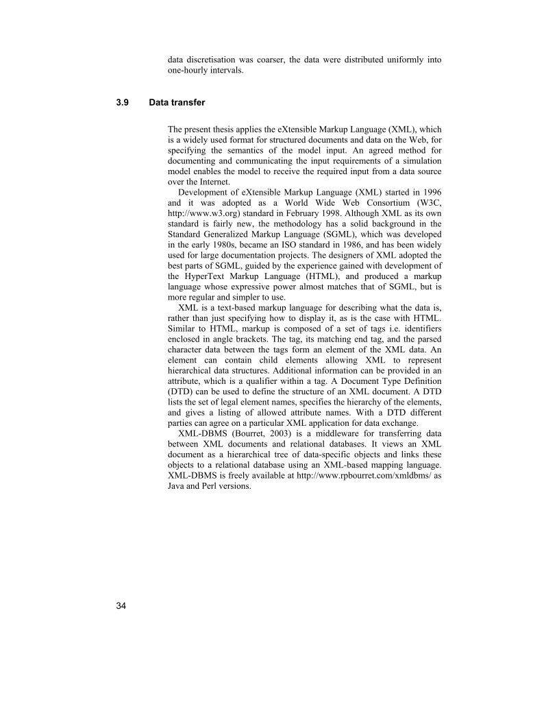
34

data discretisation was coarser, the data were distributed uniformly into one-hourly intervals.

3.9 Data transfer

The present thesis applies the eXtensible Markup Language (XML), which is a widely used format for structured documents and data on the Web, for specifying the semantics of the model input. An agreed method for documenting and communicating the input requirements of a simulation model enables the model to receive the required input from a data source over the Internet.

Development of eXtensible Markup Language (XML) started in 1996 and it was adopted as a World Wide Web Consortium (W3C, http://www.w3.org) standard in February 1998. Although XML as its own standard is fairly new, the methodology has a solid background in the Standard Generalized Markup Language (SGML), which was developed in the early 1980s, became an ISO standard in 1986, and has been widely used for large documentation projects. The designers of XML adopted the best parts of SGML, guided by the experience gained with development of the HyperText Markup Language (HTML), and produced a markup language whose expressive power almost matches that of SGML, but is more regular and simpler to use.

XML is a text-based markup language for describing what the data is, rather than just specifying how to display it, as is the case with HTML. Similar to HTML, markup is composed of a set of tags i.e. identifiers enclosed in angle brackets. The tag, its matching end tag, and the parsed character data between the tags form an element of the XML data. An element can contain child elements allowing XML to represent hierarchical data structures. Additional information can be provided in an attribute, which is a qualifier within a tag. A Document Type Definition (DTD) can be used to define the structure of an XML document. A DTD lists the set of legal element names, specifies the hierarchy of the elements, and gives a listing of allowed attribute names. With a DTD different parties can agree on a particular XML application for data exchange.

XML-DBMS (Bourret, 2003) is a middleware for transferring data between XML documents and relational databases. It views an XML document as a hierarchical tree of data-specific objects and links these objects to a relational database using an XML-based mapping language. XML-DBMS is freely available at http://www.rpbourret.com/xmldbms/ as Java and Perl versions.

35

4 RESULTS AND DISCUSSION

4.1 How to select a modelling strategy?

In Section 3 it became clear that an abundance of methods has been proposed to represent relationships between rainfall and streamflow mathematically. Many classifications for dividing rainfall-runoff models into distinct categories are available in the literature; that of Beck (1991) was presented in Section 1.2. Many models, however, do not neatly conform to any of such general categories, but rather contain elements from several modelling approaches. This is natural, as often models are tailored to suit specific case studies. Since the ‘total picture of the hydrologic system’, as phrased by Freeze and Harlan (1969), is not available, it is necessary to consider particular objectives, and also constraints imposed by availability of data and computing power, when selecting a modelling strategy.

In Paper I it is argued that when only limited data (daily rainfall, streamflow, and temperature) are available, it is difficult to justify substantial ‘conceptualisation’ of complex processes. Level of conceptualisation is understood here as the degree to which the model structure and its parameters can be related to catchment-scale hydrological processes. Increasing the level of conceptualisation enables the model to take into account various water fluxes, which are perceived to be of importance for the particular problem at hand. But, if there are no data to validate predicted water fluxes, there is a danger that the inadequacy of the model to reproduce those fluxes goes unnoticed. In Figure 11, simulated streamflow and evapotranspiration series are shown for two different model structures (for details, see Paper I). The difference in the modelled streamflow between these two models is very small, but they generate drastically different evapotranspiration time series. It is evident that streamflow data alone do not help in assessing the structural adequacy of the representation of evapotranspiration.

Figure 11. Simulated runoff and evapotranspiration series for two model structures.

As discussed in Section 2.4, models possessing physics-based process descriptions attempt to utilise data that are directly measurable in the field or in a laboratory. In Paper II a method is described as to how to incorporate topographical information into a semi-distributed rainfall-runoff model. The approach taken was to construct a flow direction grid from a digital elevation model, and then follow flowpaths from all grid cells located at the catchment border to the point where they first crossed a channel belonging to the drainage network of the catchment. Figure 12 plots the longitudinal sections for all computed flowpaths, i.e. the elevation above channel level as a function of distance along the flowpath. Three distinct groups can be identified by examining the figure, and a fourth group was formed from short flowpaths less than 60 metres in length. Within each group an average longitudinal section was calculated to represent the entire group. The proportion of the catchment area that each average longitudinal section was assumed to represent was obtained

36

by comparing the number of flowpaths belonging to each group (Figure 12).

0

5

10

15

20

25

30

0 100 200 300 400Distance f rom ditch [m]

Ele

vatio

n ab

ove

ditc

h le

vel [

m]

500 600

Profi le 1 (0.49 )Profi le 2 (0.17)Profi le 3 (0.25)Profi le 4 (0.09)

Figure 12. Surface topography for all computed flowpaths (thin lines). Typical flowpaths are shown as thick lines, and their relative shares are given in parentheses.

Only two model parameters were systematically calibrated in Paper II; one against snow water equivalent, and one against streamflow. In addition, potential transpiration was scaled by comparison of long-term sums of measured and modelled streamflow. Figure 13 shows measured and calculated streamflows for the study period. Performance of the semi-distributed model was compared against a simple lumped model (IHACRES) having five calibration parameters, and no substantial differences were found in their capabilities to simulate streamflow (Figure 13). Figure 14 plots runoff from the four identified typical profiles during springmelt 1999. It is clear that the flat profile number three produces higher peaks than the others during the first snowmelt events.

37

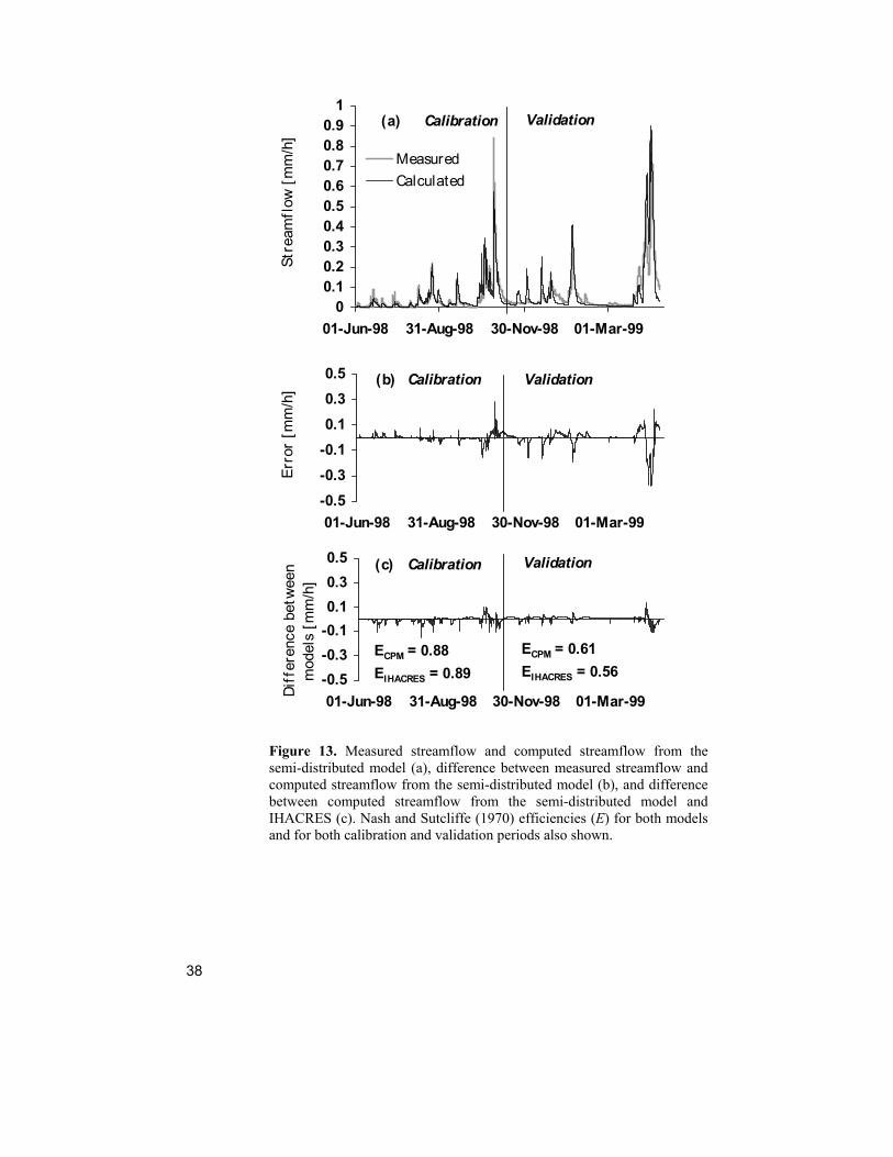
00.10.20.30.40.50.60.70.80.9

1

01-Jun-98 31-Aug-98 30-Nov-98 01-Mar-

Stre

amfl

ow [

mm

/h]

99

MeasuredCalculated

Calibration Validation

-0.5-0.3-0.10.10.30.5

01-Jun-98 31-Aug-98 30-Nov-98 01-Mar-

Erro

r [m

m/h

]

99

-0.5-0.3-0.10.10.30.5

01-Jun-98 31-Aug-98 30-Nov-98 01-Mar-Diff

eren

ce b

etw

een

mod

els

[mm

/h]

99

ECPM = 0.88EIHACRES = 0.89

ECPM = 0.61EIHACRES = 0.56

(b)

(a)

(c)

Calibration Validation

Calibration Validation

Figure 13. Measured streamflow and computed streamflow from the semi-distributed model (a), difference between measured streamflow and computed streamflow from the semi-distributed model (b), and difference between computed streamflow from the semi-distributed model and IHACRES (c). Nash and Sutcliffe (1970) efficiencies (E) for both models and for both calibration and validation periods also shown.

38

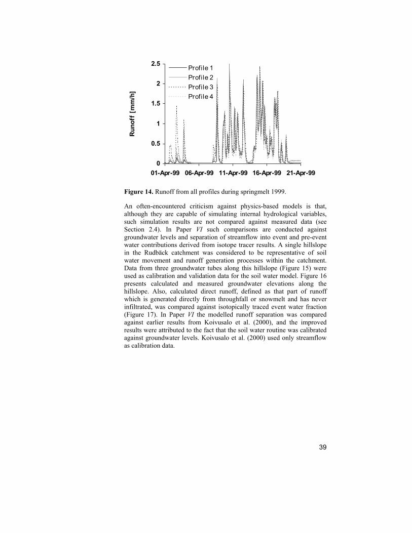
0

0.5

1

1.5

2

2.5

01-Apr-99 06-Apr-99 11-Apr-99 16-Apr-99

Run

off

[mm

/h]

21-Apr-99

Profile 1Profile 2Profile 3Profile 4

Figure 14. Runoff from all profiles during springmelt 1999.

An often-encountered criticism against physics-based models is that, although they are capable of simulating internal hydrological variables, such simulation results are not compared against measured data (see Section 2.4). In Paper VI such comparisons are conducted against groundwater levels and separation of streamflow into event and pre-event water contributions derived from isotope tracer results. A single hillslope in the Rudbäck catchment was considered to be representative of soil water movement and runoff generation processes within the catchment. Data from three groundwater tubes along this hillslope (Figure 15) were used as calibration and validation data for the soil water model. Figure 16 presents calculated and measured groundwater elevations along the hillslope. Also, calculated direct runoff, defined as that part of runoff which is generated directly from throughfall or snowmelt and has never infiltrated, was compared against isotopically traced event water fraction (Figure 17). In Paper VI the modelled runoff separation was compared against earlier results from Koivusalo et al. (2000), and the improved results were attributed to the fact that the soil water routine was calibrated against groundwater levels. Koivusalo et al. (2000) used only streamflow as calibration data.

39

Figure 15. Geometry of the hillslope in the Rudbäck catchment, locations of groundwater measurement tubes (R7, R8, and R9), and location of the interface between top and bottom soil layers.

Grou

nd w

ater

ele

vati

on [

m]

Figure 16. Measured and calculated groundwater elevations along the study hillslope in Rudbäck (tubes R7, R8, R9). Data from 1999 were used for calibration and the remaining data for validation.

40

0255075

100125150175200

01-Jan-91 02-Jul-91 01-Jan-92 01-Jul-92 31Tota

l tun

off [

mm

/mon

th]

-Dec-92-1-0.75-0.5-0.2500.250.50.751

New

water fraction [-]

Calculated runoff Measured runoff

Direct runoff fraction Event water fraction

Figure 17. Monthly total of measured and calculated runoff, and fractions of direct runoff and isotopically traced event water.

As argued in Section 1.2, and discussed further in Section 2.5, it is important to assess uncertainty inherent in the modelling results. In Section 2.6 it was pointed out that it is easier to derive statistical measures of uncertainty for simple, parsimonious models. In Paper IV, confidence intervals for instantaneous unit hydrographs have been derived over two climatically different periods of time for the same catchment, and for three different catchments over the same time period (Figures 18 and 19, respectively). Identification of the parameters defining the instant unit hydrograph has been described in detail in Papers III and IV.

The confidence intervals of IUHs shown in Figure 18 have been identified for a dry and a wet period for the same catchment (Coweeta catchment 36). The two confidence intervals do not overlap indicating that the unit hydrographs are significantly different at the 95% confidence level, and hence there appears to be some climate dependency in the model parameterisation6. However, from comparison with Figure 19 it is evident that the difference in IUHs is much smaller than in those which have been derived for the same period but for three catchments exhibiting a clearly different hydrological behaviour. In more complex models assessing implications of parametric uncertainty is harder. In Paper VI, a sensitivity analysis (Figure 20) is performed, which gives some appreciation of how much uncertain parameter values can affect modelling results.

6 Results presented later in this thesis (see Figure 21) demonstrate that IUHs for events of different intensity are variable. Results reported here address longer periods of time than single events cover. Here IUHs have been identified for time periods extending over three years.

41

Figure 18. Confidence intervals for IUHs as calibrated to Coweeta 36 catchment on two (dry and wet) time periods.

Figure 19. IUH confidence intervals for Coweeta catchments 2, 27, and 34.

42

100 300 500 700Runof f [mm]

Direct runoffRunoff from soil

(a)

0.5 0.6 0.7Depth t o GWL

0.8 [m]

(b)Reference Increase Kl Decrease Kl Increase Kv,sat Decrease Kv,sat Increase Kl Decrease Kl Increase Kv,sat Decrease Kv,sat Increase φ Decrease φ Increase θr Decrease θr Increase α Decrease α Increase β Decrease β Increase zr Decrease zr Increase fEP Decrease fEP

Bot

tom

laye

r pa

ram

eter

sTo

p la

yer

para

met

ers

Figure 20. Sensitivity of runoff components (a) and groundwater depth (b) to parameter perturbations of ±20%. CPM model application in Rudbäck. Symbols in this figure are from Paper VI and do not appear in the list of symbols (Appendix 1).

In Section 2.2 it was discussed that the unit hydrograph, i.e. the dynamics in conversion of effective rainfall into streamflow, can vary with the intensity of the event. The results of Paper V suggest that in small catchments a single instantaneous unit hydrograph may not be sufficient to adequately describe conversion of effective rainfall into streamflow, although the series of effective rainfall would be allowed to take any plausible shape. The approach taken was to optimise parameters of the instantaneous unit hydrograph and values of effective rainfall series concurrently from precipitation-streamflow data without imposing a functional form of the precipitation filter a priori. The effective rainfall was allowed to take any value as long as it did not exceed the measured rainfall at any time step. A gamma distribution function was used to parameterise the instantaneous unit hydrograph. Figure 21 plots the estimated instantaneous unit hydrographs for 9 events in Rudbäck and 17 events in Andrews Watershed 2. Instantaneous unit hydrographs are plotted in descending order of the measured event peak flows, and it is

43

easy to detect that events of greater magnitude tend to have a flashier response in both catchments. A similar relationship between event magnitude and response dynamics could not be identified in the larger catchments (58 and 1235 km2) of the study (Figure 22).

IUH

ord

inat

e [-]

Peak f low [mm/h]

Peak f low [mm/h]

IUH

ord

inat

e [-]

(a)

(b)

Rudbäck (0.

Andrews WS 2 (0.

Time 100 h

Time 100 h

18 km2)

63 km2)

Figure 21. Estimated IUHs for 9 events in Rudbäck (a) and 17 events in Andrews Watershed 2 (b). IUHs are plotted in descending order of event peak flow and the distance between starting points of IUHs is directly comparable to the difference between corresponding event peak flows. Time scale is shown as a separate line.

44

Figure 22. Estimated IUHs for 13 events in Santamäki (a) and 20 events in Myllymäki (b). IUHs are plotted in descending order of event peak flow and the distance between starting points of IUHs is directly comparable to the difference between corresponding event peak flows. Time scale is shown as a separate line.

The relationship between event magnitude and IUH parameterisation, which was detected in the smaller catchments, was exploited to formulate a structure for an event dependent (variable) IUH in Andrews Watershed 2. The scale parameter β (see Equation 15) was found to have a much stronger correlation with the event magnitude than the shape parameter α. Following this finding, the scale parameter β was related to the value of effective rainfall via a linear relationship while the shape parameter α was fixed to a constant value (see Paper V for details). Results presented in Figure 23 show that in three out of the four events selected for model validation the proposed variable IUH scheme provides a more accurate prediction of the flow hydrograph than a constant IUH scheme used as a reference.

45

Stre

amflo

w [m

m/h

]S

tream

flow

[mm

/h]

(a) (b)

(c) (d)

Observed

Constant IUH

Variable IUH

Figure 23. Observed and computed streamflows for two rainfall-runoff models involving either a variable or a constant IUH scheme. The shown four events are from Andrews Watershed 2 and are labelled in Paper V as event 1 (a), event 3 (b), event 11 (c), and event 14 (d).

In short, choice of a modelling methodology must depend on the problem at hand and on the data available. Results of this thesis (Paper II) corroborate the understanding (see e.g. Beven, 1996) that relatively simple models are adequate when the objective is to reproduce streamflow. But when it is desired to utilise measurements of internal hydrological variables, such as groundwater levels in Paper VI, a more complex model structure may be required. Despite the criticism presented against physics-based modelling (see Section 2.4), at least such models do allow model validation against internal state variables (Refsgaard et al., 1996). And when hydrological impacts of proposed land use changes are to be assessed, data representative of the changed conditions are often not available and the assessment must be based on a priori knowledge of the relevant hydrological processes. Above it was presented how topographical information can be used to form typical profiles, and it was also shown that the modelled hydrological response is different between

46

47

those profiles giving justification to the division. Similar approaches could be applied to incorporate land use data for the division of the catchment, and when changes in land use are proposed, model runs reflecting the proposed change could aid in assessing the impacts arising from the change. In any case, and particularly when there are no measurements to validate calculated hydrological fluxes, model results should be considered as an ‘expert opinion’ – not as an accurate reproduction of the real phenomena. Hence, it is important to address uncertainty contained in the results (Paper IV), and to document the modelling exercise carefully so that it is open to criticism and suggestions for improvement.

4.2 Modelling of ungauged catchments

Expert opinions and information from other catchments become especially valuable when in a particular catchment there are no flow data available to support calibration of hydrological models. In Paper III, prediction of daily streamflow using regionalisation techniques is explored using the Coweeta data.

In the light of the results it was not sufficient to adopt the mean of available calibrated parameter values as a regionalisation method for an ungauged catchment. From Figure 24 it can be seen that use of average parameters (labelled ‘Mean’ in the figure) often yields poor results in comparison to other methods. This implies that differences in the physical properties of catchments should be considered. Two regionalisation methods, Reg1Corr and NearElev in Figure 24, produced daily runoff predictions which were not much inferior to those given by calibration. The first method is a regression-based technique where correlations between runoff model parameters, i.e. dependent variables in the regressions, are also considered. And in the latter technique, a parameter set is transferred directly to the ungauged catchment from a gauged catchment likely to have a similar hydrological behaviour. Selection of such a gauged catchment was based on the weir elevation, which was identified to have a significant role in explaining the hydrological behaviour in the Coweeta basin.

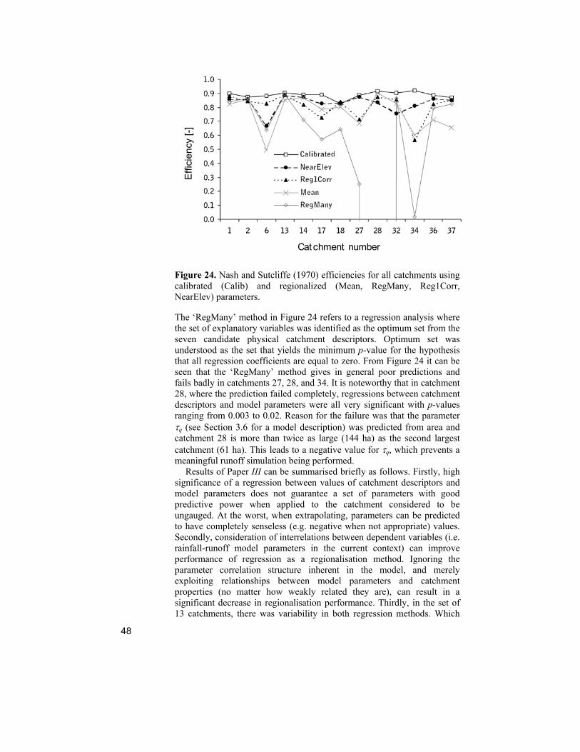
Effi

cien

cy [-

]

Cat chment number

Figure 24. Nash and Sutcliffe (1970) efficiencies for all catchments using calibrated (Calib) and regionalized (Mean, RegMany, Reg1Corr, NearElev) parameters.

The ‘RegMany’ method in Figure 24 refers to a regression analysis where the set of explanatory variables was identified as the optimum set from the seven candidate physical catchment descriptors. Optimum set was understood as the set that yields the minimum p-value for the hypothesis that all regression coefficients are equal to zero. From Figure 24 it can be seen that the ‘RegMany’ method gives in general poor predictions and fails badly in catchments 27, 28, and 34. It is noteworthy that in catchment 28, where the prediction failed completely, regressions between catchment descriptors and model parameters were all very significant with p-values ranging from 0.003 to 0.02. Reason for the failure was that the parameter τq (see Section 3.6 for a model description) was predicted from area and catchment 28 is more than twice as large (144 ha) as the second largest catchment (61 ha). This leads to a negative value for τq, which prevents a meaningful runoff simulation being performed.

Results of Paper III can be summarised briefly as follows. Firstly, high significance of a regression between values of catchment descriptors and model parameters does not guarantee a set of parameters with good predictive power when applied to the catchment considered to be ungauged. At the worst, when extrapolating, parameters can be predicted to have completely senseless (e.g. negative when not appropriate) values. Secondly, consideration of interrelations between dependent variables (i.e. rainfall-runoff model parameters in the current context) can improve performance of regression as a regionalisation method. Ignoring the parameter correlation structure inherent in the model, and merely exploiting relationships between model parameters and catchment properties (no matter how weakly related they are), can result in a significant decrease in regionalisation performance. Thirdly, in the set of 13 catchments, there was variability in both regression methods. Which

48

49

catchment descriptors were identified as explanatory variables for model parameters depended on which catchment was regarded as ungauged. The fact that the analysis was sensitive to a removal of one catchment and inclusion of another indicated that the number of available data points for the regressions was relatively small. And fourthly, when there is a reason to believe that in the sense of hydrological behaviour a gauged catchment resembles the ungauged catchment to a sufficient extent, it may be worthwhile to adopt the entire set of calibrated parameters from the gauged catchment.

An obvious drawback of the regionalisation type of methodology applied in Paper III is that flow data from numerous catchments belonging to the same region need to be available. Another way to reproduce flows for ungauged catchments is to exploit the available information on catchment properties in a more physics-based way, where there is no need to establish statistical relationships between catchment properties and parameter values of the hydrological model. As discussed in Section 2.4, there are still many problems to be tackled before physics-based models will find wider applicability. However, the results of Paper II reported in the previous Section, where a minimum amount of parameter calibration yielded satisfactory simulation results, show some promise in predicting streamflow in a physically more consistent way.

4.3 Model integration

In Paper VII methods are explored for how to transfer information between data sources and environmental simulation models in a web environment. The eXtensible Markup Language (XML) was selected as the data transfer format.

In the study application two snowmelt models, which have different process descriptions and different data requirements, were linked with a database which can be accessed over the Internet. The simpler model is based on the degree-day concept and it needs only daily precipitation and air temperature as input data. The other snow model (Koivusalo et al., 2001) is based on the energy balance approach and is much more demanding in its input data requirements. The energy balance model is driven by precipitation, air temperature, relative humidity, wind speed, and downward short- and long-wave radiation. In addition to the data input, both models require parameter values to be prescribed and given as parameter input to the models prior to a simulation. The degree-day model yields water equivalent and liquid water content of snow as a simulation output, and the energy balance model produces both snow mass and energy state variables as outputs.

In this application the focus was on the data transfer methodology, and the models did not contain any computational procedures. The meteorological data were from a meteorological station in Siuntio located in southern Finland within 50 kilometres of Helsinki. The meteorological time-series, and additional site and data specific information (metadata), were stored in a PostgreSQL (http://www.postgresql.org) relational database.

Figure 25 illustrates the linkage between the database and the snow models as perceived in the sample application. All input to the models and output from the models are directed through an interface, which accepts only XML.

Database

DB Schema

XML-DBMSMap File

Degree-Day Snow Model

DTD

Energy BalaMode

nce Snow l

DTD

XMLXML

ModelParameters

ModeParame

lters

XMLXML

Figure 25. Schematic representation of the linkage between database and snow models.

To create a simulation run, the user chooses via a Web browser which model is to be run and which data are fed to the selected model. Each model available in the system has an associated DTD file, which specifies the required data input and its structure. After the model selection has been accomplished, the user informs the system where the requested variables reside in the database. This information and the DTD file are then used to generate automatically an XML-DBMS map file. The map file describes linkage between structure of the XML document, which is required as an input to the model, and the database schema. A utility application included in the XML-DBMS package for creating map file templates from DTD files was modified to construct the map files required in this sample application. Finally, the user selects via the Web interface the site and the simulation period. This completes the information required to retrieve the model input from the database. The produced XML data file contains relevant time-series required to drive the selected model, and site-specific metadata such as site name and units of the input variables.

Figure 26a shows the DTD describing data input requirements of the degree-day snow model, and Figure 26b depicts an example of a generated input file for the degree-day snow model. For more details, including

50

description of the XML-DBMS map file, the reader is referred to Paper VII.

51

D> EQUIRED>

a) <!ELEMENT Site (Record+,AirTempUnit, PrecipUnit,SiteName)> <!ELEMENT Record (AirTemp,Precip,Date)> <!ELEMENT AirTemp (#PCDATA)> <!ELEMENT Precip (#PCDATA)> <!ELEMENT Date (#PCDATA)> <!ELEMENT AirTempUnit (#PCDATA)> <!ELEMENT PrecipUnit (#PCDATA)> <!ELEMENT SiteName (#PCDATA)> <!ATTLIST Site SiteCode CDATA #REQUIRE<!ATTLIST Record RecordNumber CDATA #R b) <?xml version="1.0" encoding="UTF-8"?> <Site SiteCode="1"> <Record RecordNumber="1"> <AirTemp>0.39</AirTemp> <Precip>2.5</Precip> <Date>Jan 1, 1997</Date> </Record> <Record RecordNumber="2"> ... </Record> <AirTempUnit>C</AirTempUnit> <PrecipUnit>mm/d</PrecipUnit> <SiteName>Siuntio</SiteName> </Site>

Figure 26. A DTD file specifying data input requirements for the degree-day snow model (a), and a data input file in XML format for the degree-day snow model (b).

52

5 CONCLUSIONS

This work is an integrative study of methods for rainfall-runoff simulation. Owing to its character the thesis addresses a range of modelling aspects, including process description considerations, problems associated with ungauged predictions, and tools for sharing data and computational procedures over the Internet. The present thesis itself is based on data sets from three continents and application of several simulation models, which adds motivation to integration aspects between model and data resources.

As Burnash et al. (1973) formulated in the context of their streamflow prediction system, the degree of effectiveness, which the user achieves in a runoff simulation study, will be dependent on the individual initiative and care with which the investigators conduct their work. This is intuitively quite obvious and the current thesis does not either claim to offer definitive, easy to follow instructions on how any particular case study should be conducted. Choice of a modelling methodology must depend on the problem at hand and on the data available. However, some principles to be taken into account when selecting methods for a rainfall-runoff study can be outlined.

Simple, but nevertheless carefully chosen, models involving a handful of calibration parameters are normally sufficient when the objective is just to simulate streamflow, and when there are historic flow data available for the calibration. This was mentioned in Section 4.1 in the light of results from Paper II. A simple model structure can also be preferred as it facilitates systematic uncertainty assessments. Paper IV (see Section 4.1) discusses how, in the case of a parsimonious model, information on parametric uncertainty can be exploited to study dependency of model parameters on different climatic periods.

A more complex model structure can be called for when assessing hydrological problems involving water quality considerations, which often necessitates explicit representation of runoff generation mechanisms and different flow pathways. In order to have confidence in simulation results of such models that have more ambitious objectives than merely to reproduce streamflow, the results should also be validated against other measured data than just flow records. In Paper I (see Section 4.1) it was clearly demonstrated that if there are no data to validate predicted evapotranspiration series, the inadequacy of the model to reproduce it might well go unnoticed. Two different model parameterisations can both yield good quality fits to observed streamflow data, but generate drastically different evapotranspiration time series. Section 4.1 also presents results from Paper VI where simulation results of a physics-based model are compared against measured data on groundwater levels and isotope tracer results. As yet there are not many studies where internal hydrological values (e.g. as groundwater levels) and environmental tracer data have been used in development and testing of physics-based rainfall-runoff models. Such data that complement standard meteorological and streamflow data are of high value when pursuing for a more realistic description of runoff generation. Further advance in hydrological understanding on how runoff is transported through the landscape is likely

53

to be a result of new innovative methods to measure more directly in the field, what are the preferential pathways of water below the soil surface.

Sufficiently long records of on-site measurements of hydrological variables, which enable proper model calibration and validation, will continue to be of high value. Still, expert opinions on hydrological problems are frequently required when there are not sufficient data available, or if the available historic data are not representative of the conditions after the studied site has undergone a change (e.g. forest logging). In Paper III (Section 4.2) a regionalisation is undertaken where relationships between physical catchment characteristics and parameter values of a hydrological model are derived, and these relationships are used to predict streamflow in a catchment assumed to be ungauged for streamflow. These results add insights into applying regionalisation as a method for predicting flows in ungauged catchments. It is demonstrated that relationships between physical catchment characteristics and parameter values are at times so weak that in a regression based analysis removal of one catchment and inclusion of another leads to a different set of explanatory variables. Results of Paper III also indicate that consideration of interrelations between rainfall-runoff model parameters themselves can improve performance of a regionalisation exercise. Ignoring the parameter correlation structure inherent in the model can result in a significant decrease in prediction accuracy. Finally, it is suggested that, instead of establishing statistical relationships between model parameters and physical catchment descriptors, it may be worthwhile to adopt the entire set of calibrated parameters from a single gauged catchment, which is believed to exhibit a similar hydrological behaviour to the ungauged catchment under study.

An obvious drawback in the regionalisation type approach to ungauged predictions is that, although the studied catchment itself can be ungauged, flow data from numerous catchments belonging to the same region need to be available. Ideally, one would wish to exploit available information on catchment properties in a more physics-based way where observed values of physical catchment properties are incorporated into the model structure and parameters directly. Unfortunately, as discussed in Section 2.4, physics-based models still face problems which are not readily solvable. However, the results of Paper II (Section 4.1), where a minimum amount of parameter calibration yielded satisfactory simulation results, show some promise in predicting streamflow in a physically more consistent way. In Paper II, a new approach for a more objective use of topographical information in the characteristic profile model of Karvonen et al. (1999) is presented. Approaches for objectively identifying typical patterns in other spatial information, such as landuse data, have a key role in applying the characteristic profile model to problems, where the study catchment is subject to proposed treatments. Research on accounting for forestry activities is currently underway.

Good quality data are essential in understanding how streamflow responds to climatic forcing. In Paper V (Section 4.1) a relationship between response dynamics and event magnitude was identified and quantified from short-interval precipitation-streamflow data measured in two small research catchments. This relationship was subsequently built into a model structure. A similar relationship was not visible in the larger

54

catchments. If such a relationship were existent it was masked by other causes leading to the variability of hydrological response between different events.

The final part of the thesis (Paper VII and Section 4.3) explores tools for distribution of environmental data sets and simulation models over the Internet. Paper VII presents a methodology how an environmental simulation model can document and communicate its input requirements, which facilitates automated retrieval of input data from a remote data source over the Internet. Such techniques, although routinely used in many web-based services (e.g. shopping, banking, library reservations), are only emerging in the environmental field. The idea is to promote openness in environmental simulation studies by providing means for data and model integration from resources published by different parties. Efficient sharing of data and methods is vital on the track towards more comprehensive and reliable assessments in environmental decision problems.

55

6 REFERENCES

Abbott, M.B., Bathurst, J.C., Cunge, J.A., O'Connell, P.E., Rasmussen, J.L., 1986. An introduction to the European Hydrology System SHE, 1: History and philosophy of a physically-based, distributed modelling system. Journal of Hydrology 87, 45-59.

Acreman, M.C., Sinclair, C.D., 1986. Classification of drainage basins according to their physical characteristics; an application for flood frequency analysis in Scotland. Journal of Hydrology 84, 365-380.

Ambroise, B., Freer, J., Beven, K., 1996. Application of a generalized TOPMODEL to the small Ringelbach catchment, Vosges, France. Water Resources Research 32, 2147-2159.

Andersen, J., Dybkjaer, G., Jensen, K.H., Refsgaard, J.C., Rasmussen, K., 2002. Use of remotely sensed precipitation and leaf area index in a distributed hydrological model. Journal of Hydrology 264, 34-50.

Aspinall, R., Pearson, D., 2000. Integrated geographical assessment of environmental condition in water catchments: Linking landscape ecology, environmental modelling and GIS. Journal of Environmental Management 59, 299-319.

Bates, B.C., 1994. Regionalisation of hydrologic data: A review - A report as part of project D2: Regionalisation and scaling of hydrologic data. Report 94/5, CRC for Catchment Hydrology, 61 pp.

Beck, M.B., 1991. Forecasting environmental change. Journal of Forecasting 10, 3-19.

Becker, A., Braun, P., 1999. Disaggregation, aggregation and spatial scaling in hydrological modelling. Journal of Hydrology 217, 239-252.

Bergström, S., Forsman, A., 1973. Development of conceptual deterministic rainfall-runoff model. Nordic Hydrology 4, 47-70.

Beven, K., 1989. Changing ideas in hydrology: the case of physically based models. Journal of Hydrology 105, 157-172.

Beven, K., 2001. How far can we go in distributed hydrological modelling? Hydrology & Earth System Sciences 5, 1-12.

Beven, K., Binley, A., 1992. The future of distributed models: model calibration and uncertainty prediction. Hydrological Processes 6, 279-298.

Beven, K.J., 1996. A discussion of distributed hydrological modelling. In: Abbott, M.B., Refsgaard, J.C. (Eds.), Distributed Hydrological Modelling. Water Science and Technology Library. Kluwer Academic Publishers, Dordrecht, pp. 255-278.

Beven, K.J., 2002. Uncertainty and the detection of structural change in models of environmental systems. In: Beck, M.B. (Ed.), Environmental Foresight and Models: A Manifesto. Developments in Environmental Modelling. Elsevier, Amsterdam, pp. 227-250.

Beven, K.J., Kirkby, M.J., 1979. A physically based, variable contributing area model of basin hydrology. Hydrological Sciences Bulletin 24, 43-69.

56

Biftu, G.F., Gan, T.Y., 2001. Semi-distributed, physically based, hydrologic modeling of the Paddle River Basin, Alberta, using remotely sensed data. Journal of Hydrology 244, 137-156.

Bishop, K.H., 1991. Episodic increases in stream acidity catchment flow pathways and hydrograph separation, University of Cambridge, Cambridge, 246 pp.

Biswas, A.K., 1970. History of hydrology. North-Holland Publishing Company, Amsterdam, 336 pp.

Blind, M.W., van Adrichem, B., Groenendijk, P., 2001. Generic Framework Water: An open modelling system for efficient model linking in integrated water management - current status, 4th International Eurosim 2001 congress “Shaping Future with Simulation”, Delft, the Netherlands. http://www.genericframework. org/download/pdf/EUROSIM_GF.pdf, accessed Jan 20, 2003.

Blöschl, G., Sivapalan, M., 1995. Scale issues in hydrological modelling: A review. Hydrological Processes 9, 251-290.

Booty, W.G., Lam, D.C.L., Wong, I.W.S., Siconolfi, P., 2001. Design and implementation of an environmental decision support system. Environmental Modelling & Software 16, 453-458.

Bourret, R., 2003. XML-DBMS: Middleware for transferring data between XML documents and relational databases. http://www.rpbourret.com/xmldbms/, accessed January 20, 2003.

Bullen, T.D., Kendall, C., 1991. 87Sr/86Sr and δ13C as tracers of interstream and intrastorm variations in water flowpaths, Catoctin Mountain, MD. Transactions, American Geophysical Union 72, 218.

Burn, D.H., Boorman, D.B., 1993. Estimation of hydrological parameters at ungauged catchments. Journal of Hydrology 143, 429-454.

Burnash, R.J.C., Ferral, R.L., McGuire, R.A., 1973. A generalized streamflow simulation system - conceptual modeling for digital computers, Joint Federal-State River Forecast Center, Sacramento, 204 pp.

Cate, H.H.ten, Lin, H.X., Mynett, A.E., 1998. A case study on integrating software packages. In: Babovic, V., Larsen, L.C. (Eds.), HYDROINFORMATICS '98. A.A. Balkema, Copenhagen, vol 1, 457-464.

Chen, S.J., Singh, V.P., 1986. Derivation of a new variable instantaneous unit hydrograph. Journal of Hydrology 88, 25-42.

Cheng, S.J., Wang, R.Y., 2002. An approach for evaluating the hydrological effects of urbanization and its application. Hydrological Processes 16, 1403-1418.

Chiew, F., McMahon, T., 1994. Application of the daily rainfall runoff model MODHYDROLOG to 28 Australian catchments. Journal of Hydrology 153, 383-416.

Crawford, N.H., Linsley, R.K., 1966. Digital simulation in hydrology: Stanford Watershed Model IV. Technical Report 39, Stanford University, California.

Ding, J.Y., 1974. Variable unit hydrograph. Journal of Hydrology 22, 53-69.

Dooge, J.C.I., 1957. The rational method for estimating flood peaks. Engineering 184, 311-313;374-377.

57

Durand, P., Robson, A., Neal, C., 1992. Modelling the hydrology of submediterranean montane catchments (Mont-Lozère, France) using TOPMODEL: initial results. Journal of Hydrology 139, 1-14.

Evans, J.P., Jakeman, A.J., 1998. Development of a simple, catchment-scale rainfall-evapotranspiration-runoff model. Environmental Modelling & Software 13, 385-393.

Farquharson, F.A.K., Meigh, J.R., Sutcliffe, J.V., 1992. Regional flood frequency analysis in arid and semi-arid areas. Journal of Hydrology 138, 487-501.

Flügel, W.-A., 1995. Delineating hydrological response units by geographical information system analyses for regional hydrological modelling using PRMS/MMS in the drainage basin of the River Bröl, Germany. Hydrological Processes 9, 423-436.

Franchini, M., Pacciani, M., 1991. Comparative analysis of several conceptual rainfall-runoff models. Journal of Hydrology 122, 161-219.

Franchini, M., Wendling, J., Obled, C., Todini, E., 1996. Physical interpretation and sensitivity analysis of the TOPMODEL. Journal of Hydrology 175, 293-338.

Freer, J., Beven, K., Ambroise, B., 1996. Bayesian estimation of uncertainty in runoff prediction and the value of data - an application of the GLUE approach. Water Resources Research 32, 2161-2173.

Freeze, R.A., 1971. Three-dimensional, transient, saturated-unsaturated flow in a groundwater basin. Water Resources Research 7, 347-366.

Freeze, R.A., 1972a. Role of subsurface flow in generating surface runoff, 1, Base flow contributions to channel flow. Water Resources Research 8, 609-623.

Freeze, R.A., 1972b. Role of subsurface flow in generating surface runoff, 2, Upstream source areas. Water Resources Research 8, 1272-1283.

Freeze, R.A., Harlan, R.L., 1969. Blueprint for a physically-based, digitally-simulated hydrologic response model. Journal of Hydrology 9, 237-258.

Gan, T.Y., Dlamini, E.M., Biftu, G.F., 1997. Effects of model complexity and structure, data quality, and objective functions on hydrologic modeling. Journal of Hydrology 192, 81-103.

Goodrich, D.C., Woolhiser, D.A., 1991. Catchment hydrology. Reviews of Geophysics, 202-209.

Grayson, R.B., Moore, I.D., McMahon, T.A., 1992a. Physically based hydrologic modeling, 1, A terrain-based model for investigative purposes. Water Resources Research 28, 2639-2658.

Grayson, R.B., Moore, I.D., McMahon, T.A., 1992b. Physically based hydrologic modeling, 2, Is the concept realistic? Water Resources Research 28, 2659-2666.

Holko, L., Lepistö, A., 1997. Modelling the hydrological behaviour of a mountain catchment using TOPMODEL. Journal of Hydrology 196, 361-377.

Huang, G.H., Liu, L., Chakma, A., Wang, X.H., Yin, Y.Y., 1999. A hybrid GIS-supported watershed modeling system. Hydrological Science Journal 44, 597-610.

Huang, G.H., Xia, J., 2001. Barriers to sustainable water-quality management. Journal of Environmental Management 61, 1-23.

58

HWED, 1994. The program of measures for water protection in river Vantaanjoki watercourse, southern Finland (in Finnish). Report A 43, Helsinki Water and Environment District (HWED), National Board of Waters and the Environment, Helsinki, 71 pp.

Hyvärinen, V., 1984. Virtaamaoloista Suomessa (in Finnish). Nro 1984:278, Vesihallitus, Helsinki, 37 pp.

Jakeman, A.J., Hornberger, G.M., 1993. How much complexity is warranted in a rainfall-runoff model? Water Resources Research 29, 2637-2649.

Jakeman, A.J., Littlewood, I.G., Whitehead, P.G., 1990. Computation of the instantaneous unit hydrograph and identifiable component flows with application to two small upland catchments. Journal of Hydrology 117, 275-300.

Jakeman, A.J., Post, D.A., Beck, M.B., 1994. From data and theory to environmental model: The case of rainfall-runoff. Environmetrics 5, 297-314.

Jensen, K.H., Mantoglou, A., 1992. Future of distributed modelling. Hydrological Processes 6, 255-264.

Johnston, P.R., Pilgrim, D.H., 1976. Parameter optimization for watershed models. Water Resources Research 12, 477-486.

Kaitera, P., 1936. Maataloushallituksen vesistötutkimukset vuosina 1929-1935 (in Finnish), Maataloushallituksen kulttuuriteknillisiä tutkimuksia N:o 1, Helsinki.

Karvonen, T., Koivusalo, H., Jauhiainen, M., Palko, J., Weppling, K., 1999. A hydrological model for predicting runoff from different land use areas. Journal of Hydrology 217, 253-265.

Kendall, C., Sklash, M.G., Bullen, T.D., 1995. Isotope tracers of water and solute sources in catchments. In: Trudgill, S.T. (Ed.), Solute Modelling in Catchment Systems. John Wiley & Sons, London, pp. 261-303.

Kite, G.W., Pietroniro, A., 1996. Remote sensing applications in hydrological modelling. Hydrological Sciences Journal 41, 563-592.

Koivusalo, H., Heikinheimo, M., Karvonen, T., 2001. Test of a simple two-layer parameterisation to simulate energy balance and temperature of a snowpack. Theoretical and Applied Climatology 70, 65-79.

Koivusalo, H., Karvonen, T., Lepisto, A., 2000. A quasi-three-dimensional model for predicting rainfall-runoff processes in a forested catchment in Southern Finland. Hydrology & Earth System Sciences 4, 65-78.

Koivusalo, H., Kokkonen, T., 2002. Snow processes in a forest clearing and in a coniferous forest. Journal of Hydrology 262, 145-164.

Koivusalo, H., Kokkonen, T., 2003. Modelling runoff generation in a forested catchment in southern Finland. Hydrological Processes 17, 313-328.

Koivusalo, H., Kokkonen, T., Karvonen, T., Lepistö, A., 1999. Modeling snow processes and streamflow generation under forest canopy and on a forest clearing. In: Oxley, L., Scrimgeour, F. (Eds.), MODSIM 99. Modelling and simulation society of Australia and New Zealand, Hamilton, New Zealand, vol 1, 147-152.

59

Kuchment, L.S., Gelfan, A.N., Demidov, V.N., 2000. A distributed model of runoff generation in the permafrost regions. Journal of Hydrology 240, 1-22.

Kuczera, G., 1983a. Improved parameter inference in catchment models, 1, Evaluating parameter uncertainty. Water Resources Research 19, 1151-1162.

Kuczera, G., 1983b. Improved parameter inference in catchment models, 2, Combining different kinds of hydrologic data and testing their compatability. Water Resources Research 19, 1163-1172.

Kuczera, G., Williams, B.J., 1992. Effect of rainfall errors on accuracy of design flood estimates. Water Resources Research 28, 1145-1153.

Lepistö, A., 1994. Areas contributing to generation of runoff and nitrate leaching as estimated by empirical isotope methods and TOPMODEL. Aqua Fennica 24, 103-120.

Lepistö, A., Kivinen, Y., 1997. Effects of climatic change on hydrological patterns of a forested catchment: a physically based modeling approach. Boreal Environment Research 2, 19-31.

Lepistö, A., Seuna, P., Bengtsson, L., 1994. The environmental tracer approach in storm runoff studies in forested catchments. In: Seuna, P., Gustard, A., Arnell, N.W., Cole, G.A. (Eds.), FRIEND: Flow Regimes from Experimental and Network Data. Braunschweig conference. IAHS Publication No. 221, 369-379.

Linsley, R.K., Crawford, N.H., 1960. Computation of a synthetic streamflow record on a digital computer. Publication 51, International Association of Scientific Hydrology, Stanford, 526-538 pp.

Littlewood, I., 2001. Practical aspects of calibrating and selecting unit hydrograph-based models for continuous river flow simulation. Hydrological Sciences Journal 46, 795-811.

Loague, K., 1990. Changing ideas in hydrology: the case of physically based models - comment. Journal of Hydrology 120, 405-407.

Mein, R.G., Brown, B.M., 1978. Sensitivity of optimized parameters in watershed models. Water Resources Research 14, 299-303.

Mimikou, M., Gordios, J., 1989. Predicting the mean annual flood and flood quantiles for ungauged catchments in Greece. Hydrological Sciences Journal 34, 169-184.

Minshall, N.E., 1960. Predicting storm runoff on small experimental watersheds. Journal of the Hydraulics Division. Proceedings of the American Society of Civil Engineers 86, 7-38.

Mustonen, S., 1963. Kesäsateiden aiheuttamasta valunnasta (in Finnish). Tiedotus 3/1963, Maataloushallituksen insinööritoimisto, Maa- ja vesiteknillinen tutkimustoimisto, Helsinki, 90 pp.

Nash, J.E., 1957. The form of the instantaneous unit hydrograph. Publication 45, International Association of Scientific Hydrology, Wallingford, 114-121 pp.

Nash, J.E., Sutcliffe, J.V., 1970. River flow forecasting through conceptual models, Part I - A discussion of principles. Journal of Hydrology 10, 282-290.

Nathan, R.J., McMahon, T.A., 1990. Identification of homogenous regions for the purposes of regionalisation. Journal of Hydrology 121, 217-238.

60

Parker, P., Letcher, R., Jakeman, A., Beck, M.B., Harris, G., Argent, R.M., Hare, M., Pahl-Wostl, C., Voinov, A., Janssen, M. et al., 2002. Progress in integrated assessment and modelling. Environmental Modelling & Software 17, 209-217.

Perrin, C., Michel, C., Andreassian, V., 2001. Does a large number of parameters enhance model performance? Comparative assessment of common catchment model structures on 429 catchments. Journal of Hydrology 242, 275-301.

Pickup, G., 1977. Testing the efficiencies of algorithms and strategies for automatic calibration of rainfall-runoff models. Hydrological Sciences Bulletin 22, 257-274.

Pilgrim, D.H., 1983. Some problems in transferring hydrological relationships between small and large drainage basins and between regions. Journal of Hydrology 65, 49-72.

Pilgrim, D.H., 1986. Bridging the gap between flood research and design practice. Water Resources Research 22, 165S-176S.

Pilgrim, D.H., Cordery, I., 1992. Flood runoff. In: Maidment, D.R. (Ed.), Handbook of Hydrology. McGraw-Hill, New York, pp. 9.1-9.42.

Post, D.A., Croke, B.F.W., 2002. Predicting hydrologic response from physio-climatic attributes: an application to ungauged sub-catchments of the Burdekin River, North Queensland. In: Rizzoli, A.E., Jakeman, A.J. (Eds.), IEMSs 2002. International Environmental Modelling and Software Society, Lugano, Switzerland, vol 1, 334-339.

Post, D.A., Jakeman, A.J., 1996. Relationships between catchment attributes and hydrological response characteristics in small Australian mountain ash catchments. Hydrological Processes 10, 877-892.

Post, D.A., Jakeman, A.J., 1999. Predicting the daily streamflow of ungauged catchments in SE Australia by regionalising the parameters of a lumped conceptual rainfall-runoff model. Ecological Modelling 123, 91-104.

Post, D.A., Jones, J.A., Grant, G.E., 1998. An improved methodology for predicting the daily hydrologic response of ungauged catchments. Environmental Modelling and Software 13, 395-403.

Potter, K.W., 1987. Research on flood frequency analysis: 1983-1986. Reviews of Geophysics 25, 113-118.

Reed, M., Cuddy, S.M., Rizzoli, A.E., 1999. A framework for modelling multiple resource management issues - an open modelling approach. Environmental Modelling & Software 14, 503-509.

Refsgaard, J.C., 1997. Parameterisation, calibration and validation of distributed hydrological models. Journal of Hydrology 198, 69-97.

Refsgaard, J.C., Storm, B., Abbott, M.B., 1996. Comment on 'A discussion of distributed hydroloigcal modelling' by K. Beven. In: Abbott, M.B., Refsgaard, J.C. (Eds.), Distributed Hydrological Modelling. Water Science and Technology Library. Kluwer Academic Publishers, Dordrecht, pp. 279-287.

Richards, L.A., 1931. Capillary conduction of liquids through porous mediums. Physics 1, 318-333.

Robson, A., Beven, K., Neal, C., 1992. Towards identifying sources of subsurface flow: a comparison of components identified by a

61

physically based runoff model and those determined by chemical mixing techniques. Hydrological Processes 6, 199-214.

Rodhe, A., 1987. The origin of streamwater traced by oxygen-18, Uppsala University, Uppsala, 73 pp.

Rodríguez-Iturbe, I., Valdés, J., 1979. The geomorphologic structure of hydrologic response. Water Resources Research 15, 1409-1420.

Rogers, C.C.M., Beven, K.J., Morris, E.M., Anderson, M.G., 1985. Sensitivity analysis, calibration and predictive uncertainty of the Institute of Hydrology Distributed Model. Journal of Hydrology 81, 179-191.

Schultz, G.A., 1993. Hydrological modeling based on remote sensing information. Advances in Space Research 13, (5)149-(5)166.

Sefton, C.E.M., Howarth, S.M., 1998. Relationships between dynamic response characteristics and physical descriptors of catchments in England and Wales. Journal of Hydrology 211, 1-16.

Sherman, L.K., 1932. Streamflow from rainfall by the unit-hydrograph method. Engineering News Record 108, 501-505.

Skaggs, R.W., 1980. A water management model for artificially drained soils, North Carolina Agricultural Research Service, Raleigh, NC, 54 pp.

Sklash, M.G., Farvolden, R.N., 1979. The role of groundwater in storm runoff. Journal of Hydrology 43, 45-65.

Smith, J.A., 1992. Precipitation. In: Maidment, D.R. (Ed.), Handbook of Hydrology. McGraw-Hill, New York, pp. 3.1-3.47.

Smith, R.E., Goodrich, D.R., Woolhiser, D.A., Simanton, J.R., 1994. Comment on "Physically based hydrologic modeling, 2, Is the concept realistic?" by R. B. Grayson, I. D. Moore, and T. A. McMahon. Water Resources Research 30, 851-854.

Snyder, F.F., 1938. Synthetic unit-graphs. Transactions, American Geophysical Union 19, 447-454.

Sorooshian, S., Gupta, V.K., 1983. Automatic calibration of conceptual rainfall-runoff models: The question of parameter observability and uniqueness. Water Resources Research 19, 260-268.

Sorooshian, S., Gupta, V.K., Fulton, J.L., 1983. Evaluation of maximum likelihood parameter estimation techniques for conceptual rainfall-runoff models: Influence of calibration data variability and length on model credibility. Water Resources Research 19, 251-259.

Stephenson, G.R., Freeze, R.A., 1974. Mathematical simulation of subsurface flow contributions to snowmelt runoff, Reynolds Creek Watershed, Idaho. Water Resources Research 10, 284-294.

Sugawara, M., Maruyama, F., 1956. A method of prevision of the river discharge by means of a rainfall model, Symposia Darcy Dijon, vol 3, 71-76.

Swank, W.T., Crossley, D.A., Jr. (Eds.), 1988. Forest hydrology and Ecology at Coweeta. Springer-Verlag, New York.

Tasker, G.D., 1982. Comparing methods of hydrologic regionalization. Water Resources Bulletin 18, 965-970.

Thiemann, M., Trosset, M., Gupta, H., Sorooshian, S., 2001. Bayesian recursive parameter estimation for hydrologic models. Water Resources Research 37, 2521-2535.

62

Todini, E., 1996. The ARNO rainfall-runoff model. Journal of Hydrology 175, 339-382.

Uhlenbrook, S., Leibundgut, C., 2002. Process-oriented catchment modelling and multiple-response validation. Hydrological Processes 16, 423-440.

Vakkilainen, P., Karvonen, T., 1982. Adaptive Rainfall-Runoff Model, SATT-I. Civil Engineering and Building Construction Series NO. 81. Helsinki University of Technology, Helsinki, 54 pp.

Vandewiele, G.L., Elias, A., 1995. Monthly water balance of ungauged catchments obtained by geographical regionalisation. Journal of Hydrology 170, 277-291.

Vehviläinen, B., 1992. Snow Cover Models in Operational Watershed Forecasting. Publications of Water and Environment Research Institute 11, National Board of Waters and the Environment, Helsinki, 112 pp.

Vertessy, R.A., Hatton, T.J., Oshaughnessy, P.J., Jayasuriya, M.D.A., 1993. Predicting water yield from a mountain ash forest catchment using a terrain analysis based catchment model. Journal of Hydrology 150, 665-700.

Wheater, H.S., Boxall, S., Wagener, S., 2002. Regionalisation of rainfall-runoff models: an application to the Thames Basin, Proceedings BHS 8th National Hydrology Symposium, Birmingham, 199-206.

Wigmosta, M.S., Vail, L.W., Lettenmaier, D.P., 1994. A distributed hydrology-vegetation model for complex terrain. Water Resources Research 30, 1665-1679.

Wiltshire, S.E., 1986. Identification of homogeneous regions for flood frequency analysis. Journal of Hydrology 84, 287-302.

Wolock, D.M., Price, C.V., 1994. Effects of digital elevation model map scale and data resolution on a topography-based watershed model. Water Resources Research 30, 3041-3052.

Ye, W., Bates, B.C., Viney, N.R., Sivapalan, M., Jakeman, A.J., 1997. Performance of conceptual rainfall-runoff models in low-yielding ephemeral catchments. Water Resources Research 33, 153-166.

Young, P.C., 1992. Parallel processes in hydrology and water quality: a unified time series approach. Jnl. Inst. of Water and Env. Man. 6, 598-612.

Young, P.C., 2001. Data-based mechanistic modelling and validation of rainfall-flow processes. In: Anderson, M.G., Bates, P.D. (Eds.), Model validation: Perspectives in Hydrological Science. J. Wiley, Chichester, pp. 117-161.

Young, P.C., 2002. Data-based mechanistic and top-down modelling. In: Rizzoli, A.E., Jakeman, A.J. (Eds.), IEMSs 2002. International Environmental Modelling and Software Society, Lugano, Switzerland, vol 1, 363-374.

Zhao, R.J., Zhang, Y.L., Fang, L.R., Xiu, X.R., Zhang, Q.S., 1980. The Xinanjiang model, Hydrological Forecasting. IAHS Publication 129, 351-356.

Zoch, R.T., 1934. On the relation between rainfall and stream flow. Monthly Weather Review 62, 315-322.

63

Zrinji, Z., Burn, D.H., 1994. Flood frequency analysis for ungauged sites using a region of influence approach. Journal of Hydrology 153, 1-21.

(Sugawara and Maruyama, 1956) (Skaggs, 1980)

APPENDIX 1 LIST OF SYMBOLS

A catchment area [m2] ai parameter of a linear system bi parameter of a linear system C differential water capacity [m-1] c model parameter (Equation 11) [m-1] c1 model parameter (Equation 9) c2 model parameter (Equation 9) [m-1] c3 model parameter (Equation 9) [m]

64

0wk

0wk

c4 model parameter (Equation 9) [m] cb constant at which kw (cb) = (Equation 12) [m] CS tracer concentration in stream water CS1 tracer concentration in source one CS2 tracer concentration in source two CMDk catchment moisture deficit at time step k [m] D thickness of the saturated zone [m] Ek evapotranspiration during a time step k [m] f modulation parameter on the rate of evapotranspiration

(Equation 12) [m] fr runoff coefficient h soil water potential [m] dH/dl groundwater table gradient i input of a linear system (continuous time) IUH instantaneous unit hydrograph k time step index kw parameter defining the rate at which catchment wetness

declines model parameter (Equation 12)

KS horizontal saturated hydraulic conductivity [mh-1] Kz vertical hydraulic conductivity [mh-1] p model parameter (Equation 10) Pk precipitation during a time step k [m] Pmax maximum rate of rainfall [mh-1] PETk potential evapotranspiration during a time step k [m]

Q sink term accounting for lateral flow in the saturated zone [h-1] Qs total stream discharge [m3h-1] Qs1 source one contribution to the total stream discharge [m3h-1] Qs2 source two contribution to the total stream discharge [m3h-1] qlat horizontal saturated flow per unit width [m2h-1] qmax maximum rate of runoff [mh-1] r impulse response S sink term accounting for transpiration in the root zone [h-1] sk soil moisture index at time step k t time [h] Tk temperature at time step k [ºC] uk input of a linear system at time step k Uk effective rainfall during a time step k [m] vq partitioning coefficient between the quick and slow stores x output of a linear system (continuous time)

65

)(qkx

)(skx

xk total output of a linear system at time step k ‘quick’ output of a system comprising two parallel stores, at

time step k ‘slow’ output of a system comprising two parallel stores, at

time step k z distance from the soil surface [m] α shape parameter of the gamma distribution function (Equation

15) αq coefficient in the equation for quick response (Equation 5) αs coefficient in the equation for slow response (Equation 6) β scale parameter of the gamma distribution function (Equation

15) βq coefficient in the equation for quick response (Equation 5) βs coefficient in the equation for slow response (Equation 6) ∆ time step interval [h] Γ gamma function τq time constant governing the rate of recession in the quick

store [h] τs time constant governing the rate of recession in the slow store

[h]

HELSINKI UNIVERSITY OF TECHNOLOGY WATER RESOURCES PUBLICATIONS

TKK-VTR-1 Järvelä, J.

Environmental river engineering and restoration: guiding principles and hydraulic performance (in Finnish).

1998.

TKK-VTR-2 Laininen, E.

Development of the Finnish Orienteering Federation’s environmental management system (in Finnish).

1998.

TKK-VTR-3 Silander, J.

Floating breakwater and environment. 1999.

TKK-VTR-4 Jolma, A.

Development of river basin management decision support systems: Two case studies. 1999.

TKK-VTR-5 Tamm, T.

Effects of meteorological conditions and water management on hydrological processes in agricultural fields:

Parameterization and modeling of Estonian case studies. 2002.

TKK-VTR-6 Koivusalo, H.

Process-oriented investigation of snow accumulation, snowmelt and runoff generation in forested sites in

Finland. 2002.

TKK-VTR-7 Kotola, J., Nurminen, J.

Kaupunkialueiden hydrologia - valunnan ja ainehuuhtouman muodostuminen rakennetuilla alueilla, osa 1:

kirjallisuustutkimus (in Finnish). 2003.

TKK-VTR-8 Kotola, J., Nurminen, J.

Kaupunkialueiden hydrologia - valunnan ja ainehuuhtouman muodostuminen rakennetuilla alueilla, osa 2:

koealuetutkimus (in Finnish). 2003.

ISBN 951-22-6576-1

ISSN 1456-2596