Rainfall extremes in some selected parts of Central and South America: ENSO and other relationships...

INTERNATIONAL JOURNAL OF CLIMATOLOGY

Int. J. Climatol. 19: 423–455 (1999)

RAINFALL EXTREMES IN SOME SELECTED PARTS OF CENTRALAND SOUTH AMERICA: ENSO AND OTHER RELATIONSHIPS

REEXAMINEDR.P. KANE*

Instituto Nacional de Pesquisas Espaciais (INPE), C.P. 515, 12201-970 Sao Jose dos Campos SP, Brazil

Recei6ed 9 September 1997Re6ised 14 August 1998

Accepted 3 September 1998

ABSTRACT

El Ninos and anti-El Ninos (La Ninas) are known to be associated with rainfall extremes in several parts of the globe.However, not all El Ninos show good associations. Recently, a finer classification of El Nino events was attempted.It was noticed that Unambiguous ENSOW (El Nino–Southern Oscillation, Warm) events (years when El Ninoexisted, and the Tahiti minus Darwin pressure difference (T−D) minima and equatorial eastern Pacific sea surfacetemperature (SST) maxima occurred in the middle of the calendar year) were very well associated with droughts inIndia and southeast Australia (Tasmania). In addition, C (cold SST, La Nina) events showed reverse effects (excessrains) in these regions. In the present paper, rainfall in selected regions in Central and South America are examined.For the Southern Oscillation Core Region (low latitudes, 155°W–167°E) and for the Gulf–Mexico region, no finerclassification was necessary. All El Ninos were associated with excess rains and all La Ninas with droughts. As inIndia and Tasmania, Unambiguous ENSOW years were associated with droughts in some parts of northeast Brazil(Ceara, Rio grande do Norte, Paraiba, Pernambuco) and excess rains in Chile and Peru. C events did not have goodassociations except in Chile and Peru, where droughts occurred. The effect of El Ninos showed some dependence onthe month of commencement. In years when El Ninos showed no effect, considerable influence of other factors (e.g.Atlantic SST on northeast Brazil rainfall) was noticed. Thus, predictions based on El Nino alone are likely to beerroneous, a fact which should be noted by the mass media. Effects of the recent El Nino of 1997–1998 are discussed.Copyright © 1999 Royal Meteorological Society.

KEY WORDS: sea surface temperature; rainfall; drought; northeast Brazil; South America; El Nino; Southern Oscillation; ENSO;La Nina

1. INTRODUCTION

During certain years, excessively warm sea water appears off the Ecuador–Peru coast. Owing to itscoincidence with the Christmas season, the phenomenon is known as El Nino (EN/the Child). It is alsoassociated with the phenomenon of the Southern Oscillation (SO), where the atmospheric pressures in thesoutheast Pacific Ocean and the Indonesian region show a see-saw motion. For example, the pressuredifference (T−D) between Tahiti (T; 18°S, 150°W) and Darwin (D; 12°S, 131°E) becomes small and goesthrough a minimum. The El Nino phenomenon is also associated with increases in the sea surfacetemperature (SST) in the equatorial eastern Pacific. However, El Ninos and the SO Index (SOI) minimado not always occur simultaneously, there are phase lags (Deser and Wallace, 1987).

It is believed that El Nino–Southern Oscillation (ENSO) phenomena tend to coincide with droughts innortheast Brazil and floods in South Brazil (Caviedes, 1973; Hastenrath et al., 1987; Rao and Hada,1990). However, as was shown in earlier communications (Kane, 1989, 1992), this relationship is ratherloose. Low correlations between SOI and northeast Brazil rainfall have also been reported by Ropelewski

* Correspondence to: Instituto Nacional de Pesquisas Espaciais (INPE), C.P. 515, 12201-970 Sao Jose dos Campos SP, Brazil;e-mail: [email protected]

CCC 0899–8418/99/040423–33$17.50Copyright © 1999 Royal Meteorological Society

R.P. KANE424

and Halpert (1987), Aceituno (1988), Rogers (1988) and Rao et al. (1993). El Nino effects (even those ofstrong ones) are not always alike; Trenberth (1993) mentions different ‘flavors’ of El Ninos. In recentpapers (Kane, 1997b,c), a finer classification of El Nino events was attempted (details given below) andit was shown that for All-India summer monsoon rainfall, for some regions in Australia and for someregions elsewhere on the globe, rainfall deficits (droughts) showed a clear association with UnambiguousENSOW (ENSOW-U) events (years when El Nino existed, and the T−D minimum and equatorialeastern Pacific SST maximum occurred in the middle of the calendar year), while floods were clearlyassociated with cold (C) SST (La Nina) events (see section 3.2). In this paper, the rainfalls for Fortalezaand other locations in northeast, east and southeast Brazil, as well as for a part of Argentina and Chilenear southern Brazil and some central American locations, are examined to determine whether anysignificant relationships can be obtained with this finer classification of El Nino events. In addition, foryears when this classification has not proven to be satisfactory, attempts are made to check whether thediscrepancies can be explained as being due to the effect of other parameters, notably the SST of thetropical Atlantic, first examined by Markham and McLain (1977) and recently by many other workers(e.g. Ward and Folland, 1991).

The purpose of the present communication is not to undertake a detailed study of the ENSOphenomenon, or to prove/disprove its being a single, coherent, global system. On the contrary the purposeis very limited, namely, to critically examine the ENSO associations with rainfall extremes in some regionsin central and south America, mainly to check propaganda by local mass media (press, radio andtelevision) regarding the so-called El Nino effects, and to emphasize that in some regions, other effectsalmost unrelated to the ENSO phenomenon can be equally, or more, important (e.g. the effects ofAtlantic temperatures on rainfall in northeast Brazil), a fact known to some workers in this field butignored by the mass media.

2. DATA

For purposes of classification, El Nino years were obtained from Quinn et al. (1978, 1987), SO index fromWright (1977, 1984) and Parker (1983) and equatorial eastern Pacific SST data from Angell (1981), as wellas further private communication and Wright (1984). Data for SST at Puerto Chicama (Peruvian coast,8°S, 80°W) from 1925 onwards were obtained privately from Dr Todd Mitchell and those for Pacific SST(El Nino regions 1+2, 3 and 4, from 1950 onwards) were obtained from the Climate Prediction Center(CPC) of the NOAA; Trenberth (1997) was also consulted. Rainfall data were obtained for northeastBrazil from SUDENE (Superintendencia do Desenvolvimento do Nordeste, Brazil; ‘Dados PluviometricosMensais’, Volumes I, II and III) for 224 stations. Data for locations near each other and having roughlysimilar average annual rainfalls were grouped together (A, B etc.), as shown by the dashed boundaries inFigure 1a, and separately for the states of Piaui, Ceara, Rio Grande do Norte, Paraiba, Pernambuco,Alagoas, Sergipe, Bahia and Minas Gerais. These were further grouped into eight regions (1, 2, . . . , 8), asshown in Table I, having annual rainfall data for 1913–1978. The location Fortaleza in Ceara had a muchlonger data series (1849 onwards) and was considered separately (FT annual rainfall in Table I). Inaddition, for a restricted region (3–8°S, 36–41°W) in the northeast, Hastenrath (1990) gave a series(March–September rainfall; HT in Table I) combining data from 27 stations. For east-northeast (ENE)Brazil (6–11°S, 35–40°W), Rao et al. (1993) obtained a series (April–July rainfall; R in Table I)combining data from 63 stations. Outside the northeast region, annual rainfall data were supplied byCENACLI (Centro Nacional de Analises Climaticas, Brazil) for three individual locations: Rio deJaneiro, Sao Paulo (east Brazil) and Porto Alegre (southeast Brazil). For an average of eight stations inCentral-East Argentina (30°S, 65°W; Figure 1b), annual data were obtained from Compagnucci andVargas (1983). In Chile, rainfall data for Santiago (33.5°S, 70.7°W), located in a central plain between acoastal range and the Andes (altitude ca. 500 m), and for Valparaiso (33.0°S, 71.6°W), a coastal city, wereobtained from Quinn and Neal (1983) and Rutllant and Fuenzalida (1991). For Peru, rainfall data werenot immediately available; therefore, as a measure of the rainfall integrated over a drainage basin in Peru

Copyright © 1999 Royal Meteorological Society Int. J. Climatol. 19: 423–455 (1999)

RAINFALL EXTREMES IN SOME SELECTED PARTS OF CENTRAL AND SOUTH AMERICA 425

roughly 7500 km2 in extent, the median discharge of the Piura River at Piura (5°S, 81°W) as given inDeser and Wallace (1987) was used. In low-latitude northern America, rainfall data for the Gulf andMexican regions (Gulf–Mexico) from Ropelewski and Halpert (1986) and Karl et al. (1994) were used.The average rainfall data of seven stations in the Southern Oscillation Core Region (4°N–1°S, 155°W–167°E) given by Wright (1984) in the form of a rainfall index, were also used.

The rainfall data chosen are those which were easily available and may not necessarily be representativeof large regions. Some are for single stations and local vagaries cannot be ruled out, while others areannual values only. Nonetheless, it is hoped that these locations display some characteristics of the regionsin question.

Figure 1. (a) Groupings of 224 stations in northeast Brazil: Piaui (PI), A–B; Ceara (CE), A–J; Rio Grande do Norte (RN), A–E;Paraiba (PB), A–D; Pernambuco (PE), A–D; Alagoas (AL), A–D; Sergipe (SE), A–D; Bahia (BA), A–F; Minas Gerais (MG), A.

(b): Map of the South American continent


R.P. KANE426

Figure 1 (Continued)

3. RELATIONSHIP WITH EL NIN0 OS (PERU–ECUADOR COAST)

3.1. All El Ninos

Kane (1997a) showed that for rainfall at Fortaleza, Ceara, in northeast Brazil, out of 46 strong andmoderate El Nino events during 1849–1992, only 21 were associated with droughts, and only 26 withnegative deviations of any magnitude (Quinn et al., 1978, 1987 and private communication). Thus, all ElNinos are not necessarily associated with droughts. In addition, in other parts of the world, e.g. India andAustralia, not all El Ninos show a clear association with droughts (Rasmusson and Carpenter, 1983).However, the finer classification outlined below showed better relationships (Kane 1997b,c).

3.2. El Ninos of the ENSOW types etc

The term ENSO is used nowadays to describe the general phenomenon of the El Nino–SouthernOscillation (see also p. 434 below). However, in the present paper, its components EN and SO are usedin their literal sense. Thus, every year was examined to check whether it had El Nino (EN; as listed inQuinn et al. 1978, 1987), and/or SOI minimum (SO), and/or warm (W) or cold (C) equatorial easternPacific SST anomalies. For SO and SST, 12-month running means were used. For several years, ENSOW



was present, the SOI showed minima and the Pacific SST was warmer. These were subdivided into twogroups—ENSOW-U where El Nino was present and the SOI minima and SST maxima were in the middleof the calendar year (May–August), and Ambiguous ENSOW (ENSOW-A) where El Nino was present,but the SOI minima and SST maxima were in the early or later part of the calendar year. In addition tothese, there were other years in which the following conditions prevailed: (i) ENSO (El Nino and SOIminima were present, but SST was neither warmer nor colder than normal); (ii) ENW, ENC (El Nino waspresent, SOI minima was not present, but SST was warm, W, or cold, C (before or after El Nino)); or (iii)EN (only El Nino was present, without SOI minima or SST maxima or minima). Some other years didnot have an El Nino and were of the following types: (i) SOW (SOI minima existed and Pacific waterswere warm); (ii) SOC, SO, W and C, where the last category C contains all anti-El Ninos, i.e. La Ninas.The types ENC and SOC seem contradictory. In fact, during these years, EN and/or SO and C did notoccur simultaneously. Either EN or SO occurred during part of the year, being followed or preceded bya cold Pacific SST, i.e. a C event. Years not falling into any of these categories were termed non-events.This classification has been prepared for all years from 1871 onwards.

With this classification, ENSOW-U events showed excellent association with droughts in All-Indiasummer monsoon (June–September) rainfall, as well as for some regional rainfalls in Australia (Kane1997b,c). Table IIa shows the rainfall characteristics for ENSOW-U, for the eight groups (1, 2, . . . , 8)—the Hastenrath (1990) group (HT) and Rao et al. (1993) group (R), located in northeast Brazil, and forindividual locations: Fortaleza, Ceara in northeast Brazil, Rio de Janeiro, Sao Paulo and Porto Alegre ineast and southeast Brazil, as well as Central Argentina, Santiago, Valparaiso, Piura River, the CoreRegion and the Gulf–Mexico Region. For comparison, All-India summer monsoon rainfall(Parthasarathy et al., 1992) and Australian (Tasmanian) rainfalls (Srikanthan and Stewart, 1991) are alsoshown. Events marked as R were selected by Rasmusson and Carpenter (1983) and later by Ropelewskiand Halpert (1987). All data were converted to normalised units. The symbols + and − indicate positive

Table I. Details of the rainfall locations

No. of S.D.LocationSymbol Geographic position Period of(%)stations data

Latitude Longitude(S) (W)

PI (A)1 7 4.5° 42.3° 27 1913–19782 1913–197826PI (B) 46.7°7.4°3

35ca. 39.0°ca. 6.0°97 1913–1978CE (A, B, C, D, E, F, G, H);3RN (A, B, C); PB (A, B); PE (B)Fortaleza 1 3.7° 38.6° 37 1849–1997FT

4 CE (I, J); PE (A) 28 ca. 7.5° ca. 40.0° 26 1913–1978RN (D, E); PB (C, D); PE (C, D)5 1913–197822ca. 35.5°ca. 7.0°24

1921–1987Normalca. 39.0°ca. 5.0°27HT Hastenrath (1990)6 29AL (A, B, C, D); SE (A, B, C, D) ca. 10° ca. 37.5° 24 1913–1978

21 ca. 10.5° ca. 40.0° 287 1913–1978BA (A, B, C, D)BA (E, F); MG (A) 15 ca. 14.0° ca. 43.0° 24 1913–19788

1914–1982Normalca. 36.0°ca. 9.0°63Rao et al. (1993)RRI 1851–197622Rio de Janeiro 43.2°22.7°1

1903–19761846.0°23.5°1SP Sao PauloPA 1Porto Alegre 30.0° 51.2° 21 1916–1985

8 ca. 30.0° ca. 65.0° 32AG 1910–1977Central Argentina1 33.5° 70.7° NormalST 1930–1988Santiago, Chile

1930–1980Normal71.6°33.0°1Valparaiso, ChileVP1 5° 81° NormalPR 1930–1983Piura, Peru

4°N–1°S7Core RegionCR 1930–1983Normal155°W–167°EGulf–Mexico 1930–1988Normalca. 90°Wca. 30°Nca. 10GM

For abbreviations see Figure 1.Normal=normalised deviations.


R.P

.K

AN

E428

Copyright

©1999

Royal

Meteorological

SocietyInt.

J.C

limatol.

19:423

–455

(1999)

Table II. Rainfall status during El Nino years of the types (a) ENSOW-U; (b) ENSOW-A; and (c) other types of El Ninos

India Australia Northeast Brazil

AI TA 1 2 3 FT 4 5 HT 6 7 8 R RI SP PA AG ST VP PR CR GM

(a) ENSOW-US 1918 I R � − � − − � − − � + � − − � � �M 1930 I R � � � � � � � � � − � − − � � � +S 1941 II 4 � � � � � � − − − − − + + � � � � � � � � �M 1951 R � − � � � � � � � + � � � − � � − + + + −S 1957 I R � − � � − − + � � + + � + + � + + − + � � �M 1965 R � − � − � + + + � � � − − � � � � � � � � �S 1972 I R � � − � − − � − − − − − − − − � + � � � � �M 1976 R + + � + − − − − � � � � � � � � � − − + � �S 1982 I R � � � � � + � � � + � +M 1987 � � − + + + � +8–10 eventsPositive deviation 1 2 3 2 1 2 2 1 3 3 2 3 4 5 6 7 5 6 5 6 7 7Negative deviation 9 8 5 6 7 8 6 7 6 5 6 5 6 4 4 2 3 2 1 0 0 1Positive/total 0.1 0.2 0.4 0.3 0.1 0.2 0.3 0.1 0.3 0.4 0.3 0.4 0.4 0.6 0.6 0.8 0.6 0.8 0.8 1.0 1.0 0.9

(b) ENSOW-AM 1914 R � � − � � � + � � � � � � � �M 1919 II + � � � � � � � − − � − � � � �M 1923 R − � � + − + − � � � − � � − − −S 1925 I R � � � + + − + − + � � � � � + � +S 1926 II � − − � � + � + � − � � − � − + �M 1931 II + + − � � � � � � � � � − + � − − − − − � +S 1940 I − � + � � + � � � � � � � − � � � − + − � �W 1948 + − + � − − − + + � + � � − � � − + − − + +M 1953 R � + � � � � � � � − � � + + � − − � + � � �S 1958 II + � � � � � � � � � � + � � − + � + + + � +W 1963 + − + � � � + − − − − � � � � + + � + − + +W 1969 R − + � − − � + � + � � � � + � � + � − − + �S 1983 II � − � � � � � � + � � �11–13 eventsPositive deviation 9 5 5 4 5 6 6 6 5 4 5 7 5 5 3 6 8 5 4 3 8 7Negative deviation 4 8 7 8 7 7 6 6 6 8 7 5 8 8 10 6 4 3 3 5 0 1Positive/total 0.7 0.4 0.4 0.3 0.4 0.5 0.5 0.5 0.5 0.3 0.4 0.6 0.4 0.4 0.2 0.5 0.7 0.6 0.6 0.4 1.0 0.9

(c) Other El NinosS 1932 EN R � − � � � � � − � � � � � � � + − − + � + +M1939 EN R � � � � − � � − − − � � � � � + � − − � + �M 1943 EN + − � − � � � � � � − − � � � � � − − � − �3 eventsPositive deviation 1 1 0 0 0 1 0 0 0 0 0 0 0 1 1 2 2 0 1 3 2 2Negative deviation 2 2 3 3 3 2 3 3 3 3 3 3 3 2 2 1 1 3 2 0 1 1Positive/total 0.3 0.3 0.0 0.0 0.0 0.3 0.0 0.0 0.0 0.0 0.0 0.0 0.0 0.3 0.3 0.6 0.6 0.0 0.3 1.0 0.7 0.7S 1917 ENC � � � � � � � + � + � + � � � �S 1973 II ENC � + � � � � � � � � + � − − + + � � − + + �2 eventsPositive deviation 2 2 2 2 2 2 2 2 1 1 2 1 1 0 1 1 2 0 0 1 1 0Negative deviation 0 0 0 0 0 0 0 0 0 1 0 1 1 2 1 1 0 1 1 0 0 1Positive/total 0.7 1.0 1.0 1.0 1.0 1.0 1.0 1.0 1.0 0.5 1.0 0.5 0.5 0.0 0.5 0.5 1.0 0.0 0.0 1.0 1.0 0.0

RA

INF

AL

LE

XT

RE

ME

SIN

SOM

ESE

LE

CT

ED

PA

RT

SO

FC

EN

TR

AL

AN

DSO

UT

HA

ME

RIC

A429

Copyright

©1999

Royal

Meteorological

SocietyInt.

J.C

limatol.

19:423

–455

(1999)

Table II. (continued)



Other EN; 5 eventsPositive deviation 3 3 2 2 2 3 2 2 1 1 2 1 1 1 2 3 4 0 1 4 3 2Negative deviation 2 2 3 3 3 2 3 3 3 4 3 4 4 4 3 2 1 4 3 0 1 2Positive/total 0.6 0.6 0.4 0.4 0.4 0.6 0.4 0.4 0.3 0.2 0.4 0.2 0.2 0.2 0.4 0.6 0.8 0.0 0.3 1.0 0.8 0.5All EN; 28 eventsPositive deviation 13 10 10 8 8 11 10 9 9 8 9 11 10 11 11 16 17 11 10 13 18 16Negative deviation 15 18 15 17 17 17 15 16 15 17 16 14 18 16 16 10 8 9 7 5 1 4Positive/total 0.5 0.4 0.4 0.3 0.3 0.4 0.4 0.4 0.4 0.3 0.4 0.4 0.4 0.4 0.4 0.6 0.7 0.6 0.6 0.7 0.9 0.8

The strengths of the El Ninos involved are indicated by: S, strong; M, moderate; and W, weak. First and second years of double events (El Ninos in two consecutive years) areindicated by I and II. The symbol R indicates that these events were also in the Rasmusson and Carpenter (1983) list. The columns show the rainfalls of: AI, All-India summermonsoon; TA, Tasmania (Australia); Regions 1, 2, 3, 4, 5, 6, 7, 8 and FT, Fortaleza; HT, the Hastenrath group; R, the Rao et al. group; all areas in northeast Brazil; RI, Riode Janeiro; SP, Sao Paulo; PA, Porto Alegre; areas in east and southeast Brazil; AG, Central Argentina; ST, Santiago; VP, Valparaiso; PR, Piura River discharge; CR, CoreRegion; and GM, Gulf–Mexico Region. The symbols + and − indicate positive and negative deviations within 0 to 90.5s, respectively, while � (positive) and � (negative)represent deviations \0.5s.

R.P. KANE430

and negative deviations within 0–0.5s, while � (positive) and � (negative) represent deviations \0.5s.As can be seen, the Indian and Tasmanian rainfalls ha6e a preponderance of negati6e de6iations. The onlyexception is 1976, probably because this El Nino began late (in April, as discussed below). Thus,ENSOW-U events show a close relationship with droughts. At the bottom of Table IIa, the numbers ofpositive and negative deviations are given. For All-India, among the ten events only one (1976) had apositive deviation and nine had negative deviations. The fraction of positive deviations was (1/10)=0.1;this fraction was also low for Tasmania (0.2). Among the other locations and groups, Fortaleza andCeara (region 3), as well as Rio Grande do Norte, Paraiba and Pernambuco (region 5) of northeast Brazilhad low fractions (0.1 and 0.2, respectively), indicating a close relationship with droughts. Regions 2, 4and 7 of northeast Brazil had a fraction of 0.3, indicating a mild association with droughts. Regions 1,6 and 8 of northeast Brazil and Rio de Janeiro, Sao Paulo and Argentina had fractions of 0.4, 0.5 and0.6 respectively, implying an almost equal number of positive and negative deviations, i.e. a poorrelationship. Porto Alegre had a fraction of 0.8, implying an association with excess rainfall, unlikenortheast Brazil. Incidentally, the deviations at Porto Alegre were not always similar to those ofArgentina, indicating that the rainfalls in and near south Brazil are not always alike. For Santiago,Valparaiso, Piura River, the Core Region and the Gulf–Mexico Region, the positive fractions are ]0.8,indicating that these places are prone to significantly higher rainfall.

Table IIb shows results for ENSOW-A. Here, Indian rainfall shows a fraction of 0.7, implying a mildaffinity for excess rains rather than for droughts. It is interesting to note that most of the II year of ElNinos fall within this group, which for India resulted in excess rainfall. Among the others, regions 2 and6 in northeast Brazil had a fraction of 0.3, i.e. a mild association with droughts. Sao Paulo had a fractionof 0.2, indicating an association with droughts. The Core and Gulf–Mexico regions showed a tendencyto flooding. All others had fractions of 0.4, 0.5 and 0.6, implying poor relationships, with the exceptionof Argentina, which had a fraction of 0.7, implying a mild tendency for excessive rainfall.

Table II(c) shows results for El Ninos of the types EN (i.e. only El Nino was present, but there wereno SOI minima or warm Pacific waters, W), and ENC (El Nino was present, but there were cold watersin the Pacific before or after the El Nino). Of the three EN events, at least two showed droughts in allregions except Porto Alegre and Argentina, where two showed excessive rainfall. At Santiago, all threeshowed a deficit in rainfall, while at Piura, all showed excessive rainfall. Thus, the pattern of droughts innortheast Brazil associated with excess rains in the south of Brazil cannot be clearly seen. In addition, therelationship with El Ninos is not invariably seen. For the two ENC-type events, a large number oflocations showed positive deviations, which for the northeast would imply an effect of C rather than EN.

At the bottom of Table II, the statistics for all 28 El Ninos types or less, indicates that only regions 2,3 and 6 of the northeast show a mild association with droughts (fraction of positives, 0.3), Argentina andPiura River for excessive rainfall (fraction of positives, 0.7) and the Core and Gulf–Mexico regions forsignificantly excessive rainfall. All other regions show poor relationships (fractions 0.4, 0.5 and 0.6).

The statistics for the various El Nino groups (a, b and c) as well as their total are given in Table V.Summarizing:

(i) The rainfall in the Core and Gulf–Mexico regions is excessive for all types of El Nino events.(ii) Only the ENSOW-U seems to show a good relationship with droughts in India, Tasmania and Ceara,

as well as nearby regions in northeast Brazil. It also shows a mild association with excess rainfall inthe south of Brazil, and a clear association with excess rainfall in Chile and Peru (Piura Riverdischarge). Thus, ENSOW-U certainly has a ‘flavor’ for more consistent ENSO relationships than doother El Nino events.

(iii) However, out of 24 El Nino years, Porto Alegre and Argentina had similar deviations for only 15years and dissimilar deviations for 9 years. Thus, rainfall may not be similar in Argentina and nearbySouth Brazil.

In northeast Brazil, Fortaleza, Ceara, has the longest rainfall record. Thus far, only data from about1913 onwards were considered. For Fortaleza alone, the results for earlier periods were as follows:



ENSOW-AENSOW-U Other El Ninos

S 1877 I � S 1878 II � ENSO S 1871+ ENW S 1884 �ENSO W 1873 � EN M 1897 �M 1896 �

S 1899 � ENSO M 1880+ ENC M 1874+ENC M 1887−ENSO S 1891 �M 1902 �

ENSO S 1990 � ENC M 1889 �M 1905−ENSO S 1912 � ENC M 1907�S 1911+

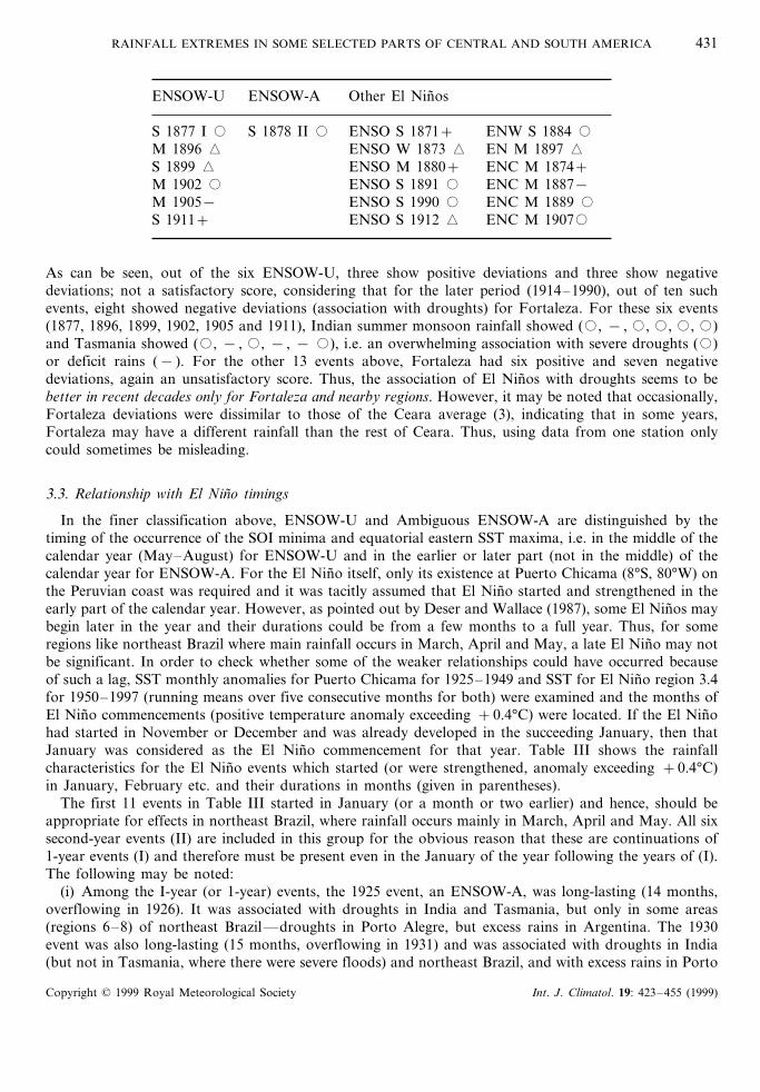
As can be seen, out of the six ENSOW-U, three show positive deviations and three show negativedeviations; not a satisfactory score, considering that for the later period (1914–1990), out of ten suchevents, eight showed negative deviations (association with droughts) for Fortaleza. For these six events(1877, 1896, 1899, 1902, 1905 and 1911), Indian summer monsoon rainfall showed (�, − ,�,�,�,�)and Tasmania showed (�, − ,�, − , − �), i.e. an overwhelming association with severe droughts (�)or deficit rains (− ). For the other 13 events above, Fortaleza had six positive and seven negativedeviations, again an unsatisfactory score. Thus, the association of El Ninos with droughts seems to bebetter in recent decades only for Fortaleza and nearby regions. However, it may be noted that occasionally,Fortaleza deviations were dissimilar to those of the Ceara average (3), indicating that in some years,Fortaleza may have a different rainfall than the rest of Ceara. Thus, using data from one station onlycould sometimes be misleading.

3.3. Relationship with El Nino timings

In the finer classification above, ENSOW-U and Ambiguous ENSOW-A are distinguished by thetiming of the occurrence of the SOI minima and equatorial eastern SST maxima, i.e. in the middle of thecalendar year (May–August) for ENSOW-U and in the earlier or later part (not in the middle) of thecalendar year for ENSOW-A. For the El Nino itself, only its existence at Puerto Chicama (8°S, 80°W) onthe Peruvian coast was required and it was tacitly assumed that El Nino started and strengthened in theearly part of the calendar year. However, as pointed out by Deser and Wallace (1987), some El Ninos maybegin later in the year and their durations could be from a few months to a full year. Thus, for someregions like northeast Brazil where main rainfall occurs in March, April and May, a late El Nino may notbe significant. In order to check whether some of the weaker relationships could have occurred becauseof such a lag, SST monthly anomalies for Puerto Chicama for 1925–1949 and SST for El Nino region 3.4for 1950–1997 (running means over five consecutive months for both) were examined and the months ofEl Nino commencements (positive temperature anomaly exceeding +0.4°C) were located. If the El Ninohad started in November or December and was already developed in the succeeding January, then thatJanuary was considered as the El Nino commencement for that year. Table III shows the rainfallcharacteristics for the El Nino events which started (or were strengthened, anomaly exceeding +0.4°C)in January, February etc. and their durations in months (given in parentheses).

The first 11 events in Table III started in January (or a month or two earlier) and hence, should beappropriate for effects in northeast Brazil, where rainfall occurs mainly in March, April and May. All sixsecond-year events (II) are included in this group for the obvious reason that these are continuations of1-year events (I) and therefore must be present even in the January of the year following the years of (I).The following may be noted:

(i) Among the I-year (or 1-year) events, the 1925 event, an ENSOW-A, was long-lasting (14 months,overflowing in 1926). It was associated with droughts in India and Tasmania, but only in some areas(regions 6–8) of northeast Brazil—droughts in Porto Alegre, but excess rains in Argentina. The 1930event was also long-lasting (15 months, overflowing in 1931) and was associated with droughts in India(but not in Tasmania, where there were severe floods) and northeast Brazil, and with excess rains in Porto


R.P

.K

AN

E432

Copyright

©1999

Royal

Meteorological

SocietyInt.

J.C

limatol.

19:423

–455

(1999)

Table III. Rainfalls for El Nino years when El Nino was strong in January, February etc.



January (14) 1925 I A � � � + + − + − + � � � � � + � +January (2) 1926 II A � − − � � + � + � − � � − � − + �January (15) 1930 I U � � � � � � � � � − � − − � � � +January (2) 1931 II A + + − � � � � � � � � � − + � − − − − − � +January (2) 1939 � � � � − � � − − − � � � � � + � − − � + �January (5) 1941 II U � � � � � � − − − − − + + � � � � � � � � �January (3) 1943 + − � − � � � � � � − − � � � � � − − � − �January (3) 1958 II A + � � � � � � � � � � + � � � + � + + + � +January (2) 1973 II C � + � � � � � � � � + � − − + + � � − + + �January (10) 1983 II A � − � � � � � � + � � �January (6) 1987 U � � − + + � +

February (5) 1932 � − � � � � � − � � � � � � � + − − + � + +February (17) 1940 A − � + � � + � � � � � � � − � � � − + − � �February (6) 1948 A + − + � − − − + + � + � � − � � − + − − + +February (9) 1953 A � + � � � � � � � − � � + + � − − � + � � �February (11) 1969 A − + � − − � + � + � � � � + � � + � − − + �February (13)1972 I U � � − � − − � − − − − − − − − � + � � � � �

March (17) 1957 I U � − � � − − + � � + + � + + � + + − + � � �March (11) 1965 U � − � − � + + + � � � − − � � � � � � � � �

April (10) 1951 U � − � � � � � � � + � � � − � � − + + + −April (11) 1976 U + + � + − − − − � � � � � � � � � − − + � �

July (5) 1963 A + − + � � � + − − − − � � � � + + � + − + +July (17) 1982 I U � � � � � + � � � + � +

Duration in months is given in parentheses. U, Unambiguous ENSOW; A, Ambiguous ENSOW; C, ENC; Blank, EN only.


Alegre and Argentina. The 1939 event was a very short-lived event (2 months) and yet was associated withdroughts in India, northeast Brazil (excluding Fortaleza proper), Chile and the Gulf–Mexico region (butnot in Tasmania), and with excess rains in Porto Alegre, Argentina, Peru and the Core Region. The 1943event was also short-lived (3 months) but caused droughts in northeast Brazil (but not in India) and PortoAlegre, and floods in Argentina, Peru and the Gulf–Mexico region. The 1987 event was relativelylong-lasting (6 months), causing droughts in India and Tasmania, but not in northeast Brazil (Fortaleza,HT, R), and floods in Chile and the Gulf–Mexico region. Thus, while some relationship with the timingof El Nino is indicated, it is not a clear-cut relationship. Opposite rainfall patterns in northeast and SouthBrazil are sometimes seen, but on other occasions, these patterns are similar.

(ii) The other events were all II-year events, four of which were short-lived. The 1926 event (2 months)rather than leading to droughts, caused flooding in many areas, including Argentina. The 1931 event (2months) did not cause droughts in India and Tasmania, but did lead to droughts in northeast Brazil anddeficit rains in the south of Brazil, and even in Chile and Peru, as well as to excess rains in the Core andGulf–Mexico regions. The 1958 event (3 months) did not result in droughts in India and Tasmania, butdid give rise to drought in northeast Brazil and to excess rains in Porto Alegre, Argentina, Chile, Peru andthe Core and Gulf–Mexico regions. The 1973 event (2 months, considered by some workers as an abortedEl Nino), rather than producing droughts, lead instead to excess rains in nearly every region, includingPorto Alegre and Argentina, Peru and the Core Region, and to deficit rains in Chile and theGulf–Mexico region. The 1941 event was relatively long-lived (5 months) and gave droughts at alllocations (India, Tasmania, northeast Brazil), perhaps because this was an ENSOW-U (the only one oftype II); however, it also led to droughts in Argentina, although not in Porto Alegre, while Chile, Peruand the Core and Gulf–Mexico regions had very heavy rains. The 1983 event was also long-lived (10months), causing droughts in Tasmania and northeast Brazil (but not in India), as well as excess rains inChile and heavy rains in Peru and the Core and Gulf–Mexico regions. Thus, ENSOW-A II-year eventsdo not cause drought in Tasmania and India (possibly even giving rise to excess rains); however, they maycause droughts in northeast Brazil—but not necessarily excess rains in South Brazil—while Chile, Peruand the Core and and Gulf–Mexico regions have heavy rains.

The next six events in Table III began in February; the 1932 and 1972 events were relatively long-lived(5 and 13 months, respectively) and gave rise to droughts in India, Tasmania and northeast Brazil, as wellas to excess rains in Porto Alegre; however, there was no extreme rainfall in Argentina. In 1932, Santiagohad deficit rains, while Valparaiso, Peru, and the Core and Gulf–Mexico regions had excess rains. In1972, all of these regions had heavy rains. The 1953 event, although long-lived (9 months), gave excessrains in India, Chile, Peru, the Core and Gulf–Mexico regions and Tasmania, and droughts in northeastBrazil; however, there were no excess rains in South Brazil. The event of 1940 was long-lived (17 months),resulting in deficit rains in India and Tasmania and in excess rains in northeast and South Brazil, as wellas the Core and Gulf–Mexico regions. The 1948 and 1969 events, relatively long-lived (6 and 11 months,respectively), showed small deviations in India, Tasmania, northeast Brazil, Chile, Peru and Argentina,droughts in Porto Alegre, and excess rains in the Core and Gulf–Mexico regions.

The next two events in Table III began in March, were long-lasting, and caused deficit rains in Indiaand Tasmania, heavy rains in Chile, Peru and the Core and Gulf–Mexico regions, and mixed rainfalls inother places. The next two events, in 1951 and 1976, started in April; the 1951 event caused droughtsalmost everywhere, while 1976 caused excess rains in India and Tasmania, deficit rains in northeast Braziland floods in South Brazil, Argentina and the Core and Gulf–Mexico regions. Finally, for the two eventsstarting in July, 1963 gave mixed results, while 1982, although starting so late, caused droughts innortheast Brazil, India and Tasmania and flooding in Porto Alegre, Chile, Peru and the Core andGulf–Mexico regions. Thus, northeast Brazilian and Indian droughts preceded El Nino.

Overall, there seems to be some connection between the starting months of El Nino and the rainfallevents occurring in the next few months; however, there are some disconcerting exceptions (rainfalls beingaffected before El Nino events). In addition, whereas rainfalls are generally opposite in northeast andSouth Brazil, sometimes both regions have similar rainfalls.


R.P. KANE434

The term El Nino has evolved in its meaning over the years. The original reference was to the annualweak, warm ocean current that runs southwards along the Peru–Ecuador coast (e.g. represented byPuerto Chicama SSTs). However, this coastal warming is often associated with a much more extensiveanomalous ocean warming up to the International Date Line. The atmospheric component tied to ElNino is the Southern Oscillation and the joint phenomenon is termed ENSO. El Nino corresponds to thewarm phase of ENSO, while the cold phase is termed La Nina. There is, however, considerable confusionin regard to the usage of these terms, with some using the term El Nino to represent the wholephenomenon, while others restrict it to the Peru–Ecuador coastal temperature increases. Aceituno (1992)gave a general review of the confusion in the terminology and Glantz (1996) gave dictionary-typedefinitions reflecting the multitude of uses of the term El Nino. At present, temperatures in fourgeographical regions are considered: El Nino 1+2 near the Peru–Ecuador coast (0°–10°S, 90°–80°W),El Nino 3 in the region (5°N–5°S, 150°–90°W) and El Nino 4 in the region (5°N–5°S, 160°–150°W). TheSSTs most-involved in ENSO are those of the Central Pacific, not those of Peru–Ecuador (Trenberth andShea, 1987; Deser and Wallace, 1987; Ropelewski et al., 1992). In recent years, Trenberth and Hoar (1996)showed that the negative correlations between SOI and SSTs exceeded −0.80 only throughout a broadregion (5°N–10°S, 180°–120°W) and called this the El Nino 3.5 region. Meanwhile, the CPC (ClimatePrediction Center, NOAA National Centers for Environmental Prediction) also introduced in theirmonthly Climate Diagnostic Bulletin, a new SST index called El Nino 3.4 for the region (5°N–5°S,170°–120°W). Using +0.4°C as a threshold for the SSTs in the El Nino 3.4 region, Trenberth (1997) gavea list of El Nino and La Nina events since 1950. It would be interesting to compare these with the SSTanomalies in the El Nino 1+2 region. Different workers seem to use El Nino years in different ways.Some consider single years, while others consider these only as double events: 1957–1958, 1982–1983 etc.In addition, some use the first years while others use the second years (Rasmusson and Carpenter, 1983;Andrade and Sellers, 1988; Heerden et al., 1988; Xavier et al., 1995). Quinn et al. (1978, 1987) mentiononly some of these as double events (events marked as I and II in Table II). Depending upon the timingof the parameter considered (e.g. rainfalls occurring early or late in the calendar year), the first or secondyear may or may not be meaningful. Table IV compares the El Nino 1+2 region SST anomalybeginnings and durations (CPC) with those of the El Nino 3.4 region as given by Trenberth (1997), usingthe same threshold of +0.4°C for both.

As can be seen, in almost all cases the El Nino 1+2 signal comes earlier by 0–5 months, and mainlyby 0–2 months. Exceptions were June 1963, September 1968, April 1982, August 1986 and June 1994,when El Nino 3.4 was reported to have started earlier (Trenberth, 1997). In addition, in some cases noEl Nino was reported near the Peru–Ecuador coast, but El Nino 3.4 developed nonetheless. These are Wevents (or, if associated with SOI decreases SO, SOW events). Thus, El Nino 3.4 is a better and morecomprehensive representation of the ENSO phenomenon. Nevertheless, in spite of their frequent waxingand waning, the El Nino 1+2 SST anomalies (or traditional El Ninos as judged from SST anomalies atPuerto Chicama) seem to be useful as early warnings. The above list of Trenberth (1997) shows onlyevents from 1950 onwards. For our classification, the SOI used was that of Wright (1977), obtained froma principle component analysis of atmospheric pressures at eight low latitude stations around the globe,as well as on the T−D pressure difference. For SST, the Wright (1984) index for the equatorial easternPacific (6°N–6°S, 180°–90°W), a similar index given by Angell (1981) and further private communication,were used. These seem to be very similar to the El Nino 3.4 anomaly indices. For 1925–1949, the El Ninooccurrences at Puerto Chicama were as shown in Table III. For earlier periods, Quinn et al. (1978)mention that the month of onset was not available for most of the early cases (during 1864–1976), anda study of recent cases showed onset times to range from January to May.

4. EVENTS NOT INVOLVING EL NIN0 O AT PUERTO CHICAMA

As mentioned by Deser and Wallace (1987), there were some years when the SOI showed minima (SO)and/or equatorial eastern Pacific waters were warmer (W) but there was no El Nino at Puerto Chicama


RA

INF

AL

LE

XT

RE

ME

SIN

SOM

ESE

LE

CT

ED

PA

RT

SO

FC

EN

TR

AL

AN

DSO

UT

HA

ME

RIC

A435

Copyright

©1999

Royal

Meteorological

SocietyInt.

J.C

limatol.

19:423

–455

(1999)

Table IV. Temperature anomalies exceeding +0.4°C (from 5-month running means) since 1950: starting month, ending month and duration, for the El Nino3.4 region (5°N–5°S, 170°–120°W) and for the El Nino 1+2 region, near the Peru–Ecuador coast. The classification from this paper for the years involved

(ENSOW etc.) is also given

El Nino 1+2 Duration Classifications from this paperEl Nino 3.4 Duration(months)(months)

April 1951–January 1952 10 August 1951–February 1952 7 1951, ENSOW-U 1952, non-eventFebruary 1953–October 1953 9 March 1953–November 1953 9 1953, ENSOW-AMarch l957–July 1958 17 April 1957–June 1958 15 1957 I, ENSOW-U 1958 II, ENSOW-AJuly 1963–November 1963 5 June 1963–February 1964 9 1963, ENSOW-A 1964, C(La Nina)March 1965–January 1966 11 May 1965–June 1966 14 1965, ENSOW-U 1966, non-eventFebruary 1969–December 1969 11 September 1968–March 1970 19 1968, W 1969, ENSOW-AFebruary 1972–February 1973 13 April 1972–March 1973 12 1972 I, ENSOW-U 1973 II, ENCApril 1976–February 1977 11 August 1976–March 1977 8 1976, ENSOW-U 1977No El Nino July 1977–January 1978 7 1977, SOW 1978, non-eventJuly 1979–January 1980 7 October 1979–April 1980 7 1979, SOW 1980, non-eventJuly 1982–November 1983 17 April 1982–July 1983 16 1982 I, ENSOW-U 1983 II, ENSOW-AOctober 1986–January 1988 16 August 1986–February 1988 19 1986, W 1987, ENSOW-UDecember 1990–July 1992 20 March 1991–July 1992 17 1991, ENSOW-A 1992, ENSOW-AMarch 1993–July 1993 5 February 1993–September 1993 8 1993, ENSOW-AOctober 1994–January 1995 4 June 1994–March 1995 10 1994, ENSOW-A 1995, ENSOW-A

R.P. KANE436

(Peru–Ecuador coast). Workers have often also included such events for ENSO studies (Shukla andPaolino, 1983; Khandekar and Neralla, 1984; Ropelewski and Halpert, 1987; Kiladis and Diaz, 1989;Mooley and Paolino, 1989; Ropelewski and Halpert, 1989). The results for such events are not shownindividually here. The general statistics are shown in Table V, with those of other types of years. If all theSOW etc. events are considered together, there is a slight bias for positives (association with floods) innortheast Brazil.

5. NON-EVENTS

If some events give results opposite to expectations, a doubt arises as to whether the relationships foundin other cases could be obtained by fluke. An important method of verification would be to observe whathappens in years when there were no ENSO effects (no El Nino, no SOI minima, no warmer (W) orcolder (C) waters in the Pacific). These years, termed as non-events, showed average results (Table V). Ascan be seen, the fractions are mainly around 0.3–0.7, indicating that such mild associations can occurrandomly, or owing to factors unrelated with ENSO. Particularly disconcerting is the fact that for manyindividual events (not shown here), many deviations were extremes (� and �). Thus, extreme rainfallscan occur without any connection with ENSO. These facts place in doubt the veracity of some of theENSO relationships discussed above.

6. COLD EVENTS (LA NIN0 AS)

In some years, Pacific waters are colder than normal. These are La Nina years, interspersed between ElNino years. The average results for these C events are shown in Table V. An examination of individualevents (not shown here) revealed that out of the 21 events, 19 were associated with positive deviations(excess rains) in India (positive/total ratio 0.9), a very good association indeed. It also confirms that theevents chosen are real cold events, many of which were also selected by Ropelewski and Halpert (1989).However, for many other rainfalls, including those in Tasmania, the fractions are 0.4, 0.5 and 0.6, i.e.there is an almost equal number of positive and negative deviations, thus implying a poor relationship. Incontrast, Chile, Peru and the Core and Gulf–Mexico regions had very low ratios of positives, indicatingsevere drought conditions during La Ninas, which is the converse of the excess rains expected during ElNinos. A strange fact was that in the years 1921, 1924, 1964 and 1967, there were widespread floods innortheast Brazil and Argentina ; in 1938, 1942, 1954 and 1970, there were widespread droughts in northeastBrazil and Argentina ; in 1922, 1934, 1971 and 1975, there were floods in northeast Brazil and droughts inArgentina ; and in 1955 and 1956, there were droughts in northeast Brazil and floods in Argentina. All ofthese conditions prevailed during C events when only floods in the northeast and droughts in Argentinaare believed to occur, thus calling into question the veracity of this popular belief. During a 20-yearperiod, Porto Alegre and Argentina had similar deviations in only 7 years (both negative in 6 years, bothpositive in 1 year). In the other 13 years, there were opposite deviations (Porto Alegre, positive;Argentina, negative in 7 years and vice versa in 6 years). Thus, the ENSO relationship during the coldphase is very weak indeed in the Brazilian and Argentinian regions considered here.

For the period from 1950 onwards, Trenberth (1997) listed the periods of La Nina as follows:

1950 CMarch 1950–February 1951, 12 months1954 C, 1955 CJune 1954–March 1956, 22 months1956 CMay 1956–November 1956, 7 months1964 CMay 1964–January 1965, 9 months

July 1970–January 1972, 19 months 1970 C, 1971 CJune 1973–June 1974, 13 months 1973 ENC (EN aborted early), 1974 SO

1975 C, 1976 ENSOW-USeptember 1974–April 1976, 20 months


RA

INF

AL

LE

XT

RE

ME

SIN

SOM

ESE

LE

CT

ED

PA

RT

SO

FC

EN

TR

AL

AN

DSO

UT

HA

ME

RIC

A437

Copyright

©1999

Royal

Meteorological

SocietyInt.

J.C

limatol.

19:423

–455

(1999)

Table V. Average rainfall status during years of the types (a) ENSOW-U; (b) ENSOW-A; (c) other types of El Ninos; (d) all El Ninos; (e) SOW etc.; (f)non-events; and (g) C events

Positive/Total India Australia Northeast Brazil


(a) ENSOW-U 0.1 0.2 0.4 0.3 0.1 0.2 0.3 0.1 0.3 0.4 0.3 0.4 0.4 0.6 0.6 0.8 0.6 0.8 0.8 1.0 1.0 0.9(b) ENSOW-A 0.7 0.4 0.4 0.3 0.4 0.5 0.5 0.5 0.5 0.3 0.4 0.6 0.4 0.4 0.2 0.5 0.7 0.6 0.6 0.4 1.1 0.9(c) Other El Ninos 0.6 0.6 0.4 0.4 0.4 0.6 0.4 0.4 0.3 0.2 0.4 0.2 0.2 0.2 0.4 0.6 0.8 0.0 0.3 1.0 0.8 0.5(d) All El Ninos 0.5 0.4 0.4 0.3 0.3 0.4 0.4 0.4 0.4 0.3 0.4 0.4 0.4 0.4 0.4 0.6 0.7 0.6 0.6 0.7 0.9 0.8(e) SOW etc. 0.5 0.4 0.6 0.7 0.5 0.7 0.5 0.4 0.6 0.6 0.7 0.7 0.7 0.3 0.3 0.5 0.5 0.6 0.3 0.4 0.4 0.4(f) Non-events 0.5 0.6 0.5 0.7 0.5 0.4 0.5 0.5 0.6 0.5 0.5 0.5 0.5 0.5 0.6 0.5 0.3 0.4 0.4 0.1 0.4 0.5(g) C (cold SST) 0.9 0.5 0.7 0.5 0.5 0.6 0.6 0.4 0.6 0.4 0.4 0.5 0.5 0.5 0.4 0.4 0.4 0.2 0.2 0.3 0.1 0.1

The columns show the rainfalls of: AI, All-India summer monsoon; TA, Tasmania (Australia); Regions 1, 2, 3, 4, 5, 6, 7, 8 and FT, Fortaleza; HT, the Hastenrath group; R,the Rao et al. group; all areas in northeast Brazil; RI, Rio de Janeiro; SP, Sao Paulo; PA, Porto Alegre; areas in east and southeast Brazil; AG, Central Argentina; ST, Santiago;VP, Valparaiso; PR, Piura River discharge; CR, Core Region; and GM, Gulf–Mexico Region.

R.P. KANE438

Figure 2. Plot of positive fractions for various rainfalls for different types of events: (a) ENSOW-U; (b) ENSOW-A; (c) other ElNinos; (d) all El Ninos; (e) SOW, SO, W and SOC; (f) non-events; and (g) C, i.e. La Ninas. The central vertical line is for a fractionof 0.5, i.e. an equal number of positive and negative deviations, implying a poor relationship. Values to the far-right imply an excessof positive deviations, i.e. an association with excess rains, while those to the far-left imply an excess of negative deviations, i.e. an

association with droughts

September 1984–June 1985, 10 months 1984 non-event, 1985 Non-eventMay 1988–June 1989, 14 months 1988 C, 1989 Non-event

Our classification for years in these intervals is also mainly C (occasionally ‘non-event’). Thus, the Cevents selected here are genuine La Ninas.

The fractions of positive deviations shown in Table V are plotted in Figure 2. The vertical line in themiddle represents a fraction of 0.5, implying equal numbers of positive and negative rainfall deviationsand hence, a poor relationship. Values falling to the far-right imply a large fraction of positive deviations,i.e. an association with floods. Values falling to the far-left imply a small fraction of positive deviations(large fraction of negative deviations), i.e. an association with droughts. The top panel (a) is forENSOW-U and the Indian summer monsoon (AI, shown with a rectangle) shows a great affinity fordroughts. Tasmania (Australia) and some parts of northeast Brazil (Fortaleza, and regions 2, 4 and 7)also show an affinity for droughts, while Porto Alegre in South Brazil, Chile (Santiago, Valparaiso) andthe Core and Gulf–Mexico regions all show an affinity for floods. The second panel (b) for ENSOW-Ashows fractions of 0.3–0.7, i.e. only mild relationships, except for the Core and Gulf–Mexico regions,which show a great affinity for floods. Panel (c) for other El Ninos does not show good relationships forIndia or Tasmania, but some regions in northeast Brazil (6, 8, HT and R), Rio de Janeiro and Chile



(Santiago, Valparaiso) show an affinity for droughts, while Core and Gulf–Mexico regions show anaffinity for floods. In Panel (d) for all 28 El Ninos, all effects are diluted (fractions 0.3–0.7, mild or poorrelationship) except for the Core and Gulf–Mexico regions, which show floods for all El Ninos. In Panel(e) for events when there were no El Ninos, but there were events of the types SOW, SO, W and SOC,Rio de Janeiro and Sao Paulo show a mild association with droughts, while some parts of northeast Brazil(R, Fortaleza, regions 2, 7 and 8) show a mild association with floods. Panel (f) for non-events shows anaffinity for floods in region 2 of northeast Brazil and droughts in Argentina and Peru, indicating thatthese can occur for reasons unrelated to ENSO. Finally, Panel (g) for C events (La Nina) shows a goodassociation with floods in India (AI) and droughts in Chile, Peru and the Gulf–Mexico region, but noclear associations in other areas. Thus, only ENSOW-U events show good associations with droughts innortheast Brazil and floods in South Brazil (Porto Alegre). For all other types of events, the relationshipsare poor. However, the core and Gulf–Mexico regions show excess rains for all El Ninos and droughtsfor all La Ninas.

The classification used in this study (ENSOW etc.) was made by a visual inspection of the plots(12-month running means), as shown in Kane (1997b,c), and is somewhat subjective. Thus, some eventswhere SO minima or W were considered as being late or early in the calendar year (not in the middle) andtherefore were termed as ENSOW-A could just as well have been ENSOW-U. Some events in C maydeserve to be termed non-events; by and large however, the classification seems clear enough and the mainconclusion that only some parts of northeast Brazil show an association with droughts during ENSOW-Uonly and that during all other events the effects are uncertain, seems valid. This indicates that otherfactors unrelated to ENSO must be causing considerable interference, except in the Core and Gulf–Mex-ico regions, where the ENSO relationship is very strong.

7. INTERCORRELATION

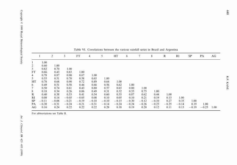
Since the different series show different results, it is obvious that these are not well related to each other.To obtain a quantitative estimate of their interrelationships, correlation coefficients were calculatedbetween the various locations in Brazil and Argentina and the matrix is shown in Table VI.

As can be seen, the northeast Brazil series are fairly well correlated (+0.5 or more) between each other;however they have a low positive correlation with Rio de Janeiro, a low negative correlation with SaoPaulo, a slightly more negative correlation with Porto Alegre, and a low positive correlation withArgentina. Rio de Janeiro has a correlation of +0.35 with Sao Paulo, −0.14 with Porto Alegre and+0.13 with Argentina. Sao Paulo has a correlation of +0.19 with Porto Algere and −0.19 withArgentina. Porto Alegre has a correlation of −0.25 with Argentina. Thus, in eastern and southern Brazil,the rainfall characteristics change rapidly with latitude, have very small intercorrelations and cannotpossibly have similar relationships with any phenomenon like ENSO.

8. RELATIONSHIP WITH FACTORS OTHER THAN ENSO

In every part of the globe, rainfalls are affected by factors which may not be related to ENSO, such aslocal conditions (circulations, topography), SSTs in nearby regions etc. For central Chile (30–35°S),Rubin (1955) found that the precipitation was below normal during the positive phase of the SO, i.e. whenthe southeast Pacific subtropical anticyclone was stronger than average (see also Pittock 1980). Quinn andNeal (1983) reported a good correlation between Chilean rainfall and SSTs in the southeastern TropicalPacific. Aceituno (1987) concluded that the excess rainfall in Chile during the negative phase of the SOwas associated with a weak and northerly displaced southeast Pacific subtropical anticyclone. Rutllantand Fuenzalida (1991) reported that the winter (June, July, August; JJA) rainfall in central Chile showedpositive anomalies during the developing stage of warm events of the SO and dry conditions during thecold events. They also presented a synoptic characterization of major storms during some warm events


R.P

.K

AN

E440

Copyright

©1999

Royal

Meteorological

SocietyInt.

J.C

limatol.

19:423

–455

(1999)

Table VI. Correlations between the various rainfall series in Brazil and Argentina

1 2 3 FT 4 5 HT 6 7 8 R RI SP PA AG

1 1.002 0.60 1.003 0.82 0.70 1.00FT 0.66 0.43 0.83 1.004 0.78 0.87 0.90 0.67 1.005 0.55 0.51 0.70 0.58 0.65 1.00HT 0.78 0.68 0.90 0.72 0.89 0.64 1.006 0.49 0.51 0.58 0.44 0.66 0.56 0.62 1.007 0.50 0.74 0.61 0.43 0.80 0.57 0.65 0.80 1.008 0.18 0.54 0.26 0.06 0.49 0.31 0.32 0.55 0.75 1.00R 0.40 0.38 0.53 0.41 0.54 0.60 0.55 0.87 0.62 0.44 1.00RI 0.08 0.14 −0.05 −0.05 0.08 0.10 0.05 0.10 0.21 0.19 0.13 1.00SP −0.11 −0.08 −0.21 −0.19 −0.18 −0.10 −0.15 −0.30 −0.12 −0.10 0.27 0.35 1.00PA −0.38 −0.31 −0.24 −0.21 −0.31 −0.14 −0.24 −0.24 −0.26 −0.23 −0.25 −0.14 0.19 1.00AG 0.16 0.24 0.22 0.22 0.22 0.28 0.18 0.19 0.20 0.12 0.11 0.13 −0.19 −0.25 1.00

For abbreviations see Table II.


and described dry months during cold events in terms of average 500 hPa contour anomaly fields, but insome cases found significant departures from the general behaviour. For central Chile, Rutllant andFuenzalida (1991) mention that the precipitation is almost exclusively a southern winter phenomenon,associated with the extratropical disturbances penetrating the area of influence of the southeast Pacificsubtropical anticyclone. About 80% of the annual precipitation occurs during May–August, distributedinto relatively few large events, particularly in wet winters. Regarding latitudes further south, Quinn andNeal (1983) mention that the prominent ENSO-related rainfall departures are primarily confined to theChilean subtropics, and that at times, stations near 40°S latitude register these changes, but to a lesserdegree.

For India, relationships were reported with Eurasian snow cover (Hahn and Shukla, 1976; Dey andBhanukumar, 1983), the state of the troposphere at middle and upper levels (Bhalme et al., 1986),stratospheric wind quasi-biennial oscillation (Bhalme et al., 1987 and references therein), and latitudinallocation of the axis of the 500 hPa ridge along 75°E (Krishna Kumar et al., 1992 and references therein).For Australia, a relationship was found with SST in the Indonesian region and Central Indian Ocean(Streten, 1983; Nicholls, 1989).

For rainfall in Brazil, particularly in the northeast, east and southern region, several factors are knownto be relevant. Markham and McLain (1977) reported considerable influence of tropical Atlantic SST.Other factors are, the 700 mb circulation pattern over the North Atlantic (Namias, 1977), the meridionaldisplacement and strength of the Inter-tropical Convergence Zone (ITCZ) (Hastenrath and Heller, 1977),Atlantic trade winds (Chung, 1982), rainfall systems associated with tropical disturbances movingwestward from the Atlantic towards northeast Brazil (Ramos, 1975; Yamazaki and Rao, 1977; Rao et al.,1993), and Southern Hemisphere cold fronts or their remains moving northward along the eastern andnortheast coast of Brazil (Kousky and Chu, 1978; Kousky, 1979). There is a well-defined large-scaleatmospheric circulation pattern related to the SST anomalies in the Tropical Atlantic (Hastenrath andHeller, 1977; Moura and Shukla, 1981). According to Hastenrath (1990), droughts in northeast Brazil canbe due to an anomalously far northerly position of the ITCZ, reduced northeast trades and acceleratedcross-equatorial flow from the Southern Hemisphere, and anomalously warm surface waters in a zonalband across the Tropical North Atlantic, contrasting with negative SST anomalies south of the equator.The association with SO minima may come about through the displacement of the near-equatorial troughnorthward. Hastenrath et al. (1984) and Hastenrath (1990) formulated prediction schemes involving zonaland meridional wind components over limited areas of the Equatorial Atlantic, SST in Tropical Northand South Atlantic, SOI and preseason rainfall itself in northeast Brazil as predictors. A particularlyinteresting aspect is the relationship between the rainfall in northeast Brazil and the coastal wind in thatregion, through its effect on the positioning of the ITCZ. Servain and Seva (1987) indicated that theposition of ITCZ was well-related to the minimum of the meridional component of the wind stress. Xavierand Xavier (1997) utilised this relationship for locating the position of the ITCZ in individual months andfor the predictions of rainfall. Since years when El Nino and cold events did not yield the expected results(droughts and floods, respectively) have been isolated here, the possibility of whether in these years otherfactors played a more important role will now be examined.

Figure 3 shows a plot of various parameters for 1913–1951 in Figure 3a and for 1952–1990 in Figure3b. The rectangles at the top show the category of the year (ENSOW etc.) allotted for this work, and inthe case of El Nino being present, the symbols above the rectangles (S, strong; M, moderate; W, weak)indicate the strength of the El Nino.

The next three plots are for rainfall at Fortaleza and for the average series by Hastenrath (1990) fornortheast Brazil and Rao et al. (1993) for east-northeast Brazil. Following these are plots of SST andzonal (U) and meridional (V) wind components in the Atlantic. Hastenrath (1990) presented indices ofJanuary values of SST, as well as and meridional and zonal wind components obtained by an EmpiricalOrthogonal Function (EOF) analysis of data for the entire Tropical Atlantic (30°N–30°S, 0–50°W). Raoet al. (1993) studied SST in the whole Atlantic and found the best correlation for a region near 10°S,10°W. They also found good correlations with the meridional wind component at Abrolhos (18°S, 39°W).Both of these sets of data have been used here, as have SST data given in Servain (1991) for the North


R.P. KANE442

Atlantic (28–5°N, 10–60°W) and South Atlantic (5°N–20°S, 10°E–40°W) and SST data for (8°S–0°W)and SST and wind stress data near the northeast Brazil coast (ca. 5°S, 40°W; Servain and Lukas (1990)and Drs Vianna and Servain, private communication). A large part of the Atlantic data were availablefrom 1964 onwards only (Figure 3b).

Figure 3. Categories of years (EN, SO etc.), rainfalls for Fortaleza (FT), the Hastenrath (1990) group (HT), and the Rao et al.(1993) group (R), and Atlantic SST and wind components (zonal, U; meridional, V) for (a) 1913–1951 and (b) 1952–1990



As mentioned earlier, among the 24 events involving El Nino and another seven involving SO and/orW, all of which were expected to be associated with droughts, at least eight were associated withunexpected flooding in northeast Brazil. These were 1914, 1926 II, 1940 I and 1969 in the El Nino group(Table II) and 1913, 1977, 1974 and 1968 in the SO/W group. These years should be examinedindividually for associations with SST and wind components in the Atlantic. Similarly, from the 21 Cevents which were expected to be associated with floods, 7 years (1928, 1938, 1942, 1954, 1955, 1956 and1970) were associated with droughts and require similar examination, as do some non-events which ratherthan giving rise to normal rainfall as expected, caused droughts or floods.

Table VII shows the results. The years, their categories (EN, SO etc.) and the expected and observedrainfalls are indicated. The symbols (+ + ), (+ ), (0), (− ) and (− − ) indicate the status of the variousSST and wind components. Thus, (+ + ) in SST (HT) means that for that year, the SST plot ofHastenrath (1990), reproduced in Figure 3, had a large positive deviation in Atlantic SST, which isfavourable for excess rainfall in northeast Brazil. A (+ + ) result also implies large positive deviations forall other SSTs except the Servain SST for the North Atlantic, for which—because of its dipole naturewith respect to the South Atlantic—a reverse convention, i.e. negati6e temperature deviations areconsidered as having a (+ ) or (+ + ) effect, are adopted. Since data for many of these parameters areavailable only from 1964 onwards, there are many gaps in the data in Figure 3a. However, in general,when floods and droughts were observed, there was a preponderance of (+ ) and (− ) respectively, thusconfirming that in cases where El Ninos and cold events did not give the expected results, the effects ofAtlantic (particularly South Atlantic) SST and winds comprised a predominant contribution.

Figure 3 shows rainfall data for Fortaleza, HT and R for years up to 1987. During 1979–1987, years1979 (SOW), 1982 (ENSOW), 1983 (ENSOW) and 1987 (ENSOW) were expected to yield droughts anddid so. However, 1980, 1981, 1984 and 1985 were non-events and 1986 was a late W; these were associatedwith droughts and floods, respectively. The lower part of Table VII shows a preponderance of negatives(− ) for droughts and positives (+ ) for floods, again indicating the prominent roles of South AtlanticSSTs and winds.

Since 1964 when copious data for the various parameters are available, only 3 years of the C type (1964,1967 and 1973) expected to have floods, did have floods and only 2 years of the ENSOW type (1982 and1983) expected to have droughts, did have droughts. Table VII (bottom) shows the contribution of otherparameters. The floods were associated mostly with (+ ) and the droughts mostly with (− ) thusaccentuating the El Nino and La Nina effects.

Therefore, it would seem that on occasions when El Ninos and La Ninas did not yield the expectedresults, considerable complications from the Atlantic region were involved. Hence, predictions in relationto rainfall anomalies in northeast Brazil must be made by taking into account the conditions in both thePacific and the Atlantic, although the media seems to be concerned only by the Pacific events (El Ninos).Such efforts are underway at present and involve correlation analysis discussed in the next section.

9. CORRELATIONS WITH PACIFIC AND ATLANTIC PARAMETERS

Ward and Folland (1991) investigated the relationship between northeast rainfall and SST in variousregions. For the Atlantic, they reported correlations similar to those reported earlier by Markham andMcLain (1977), i.e. positive correlation with SST in the South Tropical Atlantic and negative correlationwith SST in the North Tropical Atlantic. For the Tropical Pacific, negative correlations extended over awide area, thus implying a relationship with the ENSO phenomenon, reported earlier by Covey andHastenrath (1978). Furthermore, they calculated the covariance eigenvectors for SST in the Atlantic andPacific Oceans, with the main purpose being to derive a few time series which would express much of thelarge-scale variability in the SST in these two oceans. They also studied the relationship of the variouseigenvectors with north northeast Brazil rainfall. Atlantic eigenvector 3 and Pacific eigenvector 1 showedthe best correlations and together explained about 55% of the rainfall variance. When SST data wereaveraged over November–January, 35–50% of the variance was explained, sufficient to provide a


R.P

.K

AN

E444

Copyright

©1999

Royal

Meteorological

SocietyInt.

J.C

limatol.

19:423

–455

(1999)

Table VII. Indications as to whether the signs and strengths of the various Atlantic SST and wind components (zonal, U; meridional, V) forJanuary, February and March were favourable for heavy floods (++), mild floods (+), normal rainfall (0), mild droughts (−), severe

droughts (−−) in northeast Brazil

Year Type Rainfall SST U V

Expected Observed HT R SER, N SER, S VIA Off VIA Coast HT VIA HT R

1913 SOW Drought Flood1914 ENSOW Drought Flood1926 II ENSOW Drought Flood −1940 I ENSOW Drought Flood −− 01965 ENS OW Drought Flood 0 + + 0 −− − + + − ++1969 ENSOW Drought Flood − + − + + + + + 0 ++1974 SO Drought Flood + + + + + + 0 + + +1977 SOW Drought Flood + + + − 0 + 0 + + 0

1917 ENC Normal Flood1935 SOC Normal Flood ++ + +1947 X Normal Flood 0 − 0 0

1915 X Normal Drought1928 C Floods Drought −1938 C Flood Drought 01942 C Flood Drought − −1954 C Flood Drought 0 −1955 C Flood Drought + −1956 C Flood Drought −− −1970 C Flood Drought − − − − − + + − − 0

1980 X Normal Drought 0 − − − − − − − −1981 X Normal Drought − − − − − − − 0 01984 X Normal Flood + 0 + + + 0 + ++1985 X Normal Flood + 0 + + + − + +1986 W Normal Flood + + 0 + − − + +

1964 C Flood Flood − + − + + + + + 0 +1967 C Flood Flood − + − + + + + + − +1973 C Flood Flood − ++ 0 + + + 0 + + −

1982 ENSOW Drought Drought − − − 9 − −− − − −1983 ENSOW Drought Drought + − − 9 − − − + −

HT, Hastenrath (1990); R, Rao et al. (1993); SER (N, S), northern and southern Atlantic, Servain (1991); VIA (Off, Coast), coastal and off-coast, Dr Vianna(private communication). X, Non-event.


preliminary forecast of the March–April rainfall over northeast Brazil. Using two statistical techniques,namely multiple linear regression (MIR) and linear discriminant analysis (LDA), forecasts were made for1987, 1988, 1989 and 1990 which were subsequently found to be good. Since 1990, forecasts have beenavailable in February. Here, the results of a simplistic correlation analysis are reported.

In the Atlantic region, SST variations are dissimilar in the northern and southern hemispheres. SSTindices for the northern (N; 28°–5°N) and southern (S; 5°N–20°S) Atlantic were obtained from Servain(1991). Their average (N+S)/2 represents the average Tropical Atlantic SST, while their difference (N–S)represents the dipole inducing a meridional circulation cell with subsidence over northeast Brazil, asenvisaged by Moura and Shukla (1981). Two additional parameters were also considered, namely SSTvariations near the northeast Brazil coast and the zonal pseudo-wind stress (product of the intensity of theeastward wind velocity and the total wind speed) in the same region. A cross-correlation betweenFortaleza rainfall (12-month running means, centered 3 months apart) showed maximum correlations 0.30with North Atlantic SST N, 0.45 with South Atlantic SST S, 0.40 with (N+S) and (N−S), 0.50 withBrazil coastal SST and 0.40 with coastal wind stress. Thus, all of these parameters have some relationshipwith northeast Brazil rainfall. Most of these had a zero lag with rainfall, and therefore could not be usedfor prediction. However, N and S showed maximum correlation not at zero lag, but a lag of few (two tothree) seasons, with the parameters preceding the rainfall. Thus, the December–January Atlantic SSTwarming could be indicative of excess rainfall later in northeast Brazil. The equatorial eastern Pacific SSTshowed a good correlation (0.6590.05) with North Atlantic SST N, a smaller correlation (0.4590.06)with South Atlantic SST S and a moderate correlation with northeast coastal Brazil SST (−0.5, with alag of three to four seasons).

The maximum correlations (at a ca. two-season shift) between Fortaleza rainfall and Atlantic S,Atlantic N, SOI (T−D), and equatorial eastern Pacific SST were 0.52, 0.32, 0.25 and 0.18, respectively.When the Fortaleza rainfall values were shifted by two seasons and a multiple regression analysis wascarried out, the single variable correlation +0.52 between rainfall and South Atlantic SST S increased toa multiple correlation +0.69 when North Atlantic SST N was also included, but remained near +0.69when (T−D) and equatorial eastern Pacific SST were included one by one. Thus, Atlantic SST (both Nand S) seem to be the parameters of major influence, the effects of (T−D) and Pacific SST being almostinsignificant. When rainfall was correlated with northesat coastal SST and wind stress, the bivariateanalysis gave a multiple correlation +0.76, which increased to +0.80 when SST Atlantic S was alsoincluded. However, as mentioned earlier, the coastal parameters attain maximum correlations during therainfall regime and hence have no prediction potential. Overall, above-average temperatures in theTropical South Atlantic can cause excess rains in northeast Brazil and, if there is a simultaneous El Ninoeffect (droughts), normal rainfall may be the net result. However, below-normal temperatures in theTropical South Atlantic accompanied by El Nino could cause disastrous droughts in northeast Brazil.

Since the correlations are only ca. 0.7, the variance explained is ca. 50%, leaving almost 50% as arandom component. Therefore, quantitative predictions based only on Atlantic temperatures may not bevery accurate or reliable. Hastenrath et al. (1984) and Hastenrath (1990) conducted a stepwise multipleregression analysis, using October–January northeast rainfall, January values of SO (T−D pressure),Pacific and Tropical Atlantic SST and Tropical Atlantic wind components as predictors for theMarch–September northeast rainfall. In the Atlantic, the area chosen by the above authors is rather large(30°N–30°S) and EOF analysis was used; among the first five EOFs, those with the best correlation wereselected. However, the SST patterns in the North and South Atlantic are not alike; as illustrated inServain (1991), there is a meridional dipole structure, but the north (28°–5°N) and the south (5°N–20°S)series are not out of phase simultaneously. From the patterns seen in Table VII, it seems that use of SSTand winds in the South Atlantic only would be more appropriate. However, in their earlier publication,Hastenrath and Heller (1977) reported that the rainfall anomalies in northeast Brazil were associated withmeridional surface pressure gradients and the associated interhemispheric SST gradients, rather than withpressure and SST over either the Tropical North or South Atlantic alone. In a recent communication,Hastenrath and Greischar (1993) elaborated their list of predictors and showed that whereas excessrainfall in northeast Brazil was related both to anomalously cold SST and high pressure in the North


R.P. KANE446

Atlantic, and to anomalously warm SST and low pressure in the South Atlantic, the relationship ofnortheast rainfall extremes with the interhemispheric gradients of SST and pressure was even stronger.Servain (1991) gave the indices for SST variability separately for the North (NB) and South (SB) Atlantic,as well as for their difference (NB−SB) as a dipole index. However, the main feature of this dipole indexwas not a large year-to-year variation but a slow variation on a decadal time scale, i.e. positive during1964–1970 and 1976–1983 and negative during 1971–1975 and after 1984. It is clear that such a slowvariation cannot be related to the abrupt year-to-year changes in rainfall (Figure 3) seen in northeastBrazil. Earlier, Hastenrath (1990) mentioned that a model involving October–January rainfall Atlanticmeridional wind and equatorial Pacific SST as predictors captured ca. 70% of the March–Septemberrainfall variance. It would be interesting to see whether the modified list of predictors used by Hastenrathand Greischar (1993) (including N–S gradients) explains variance exceeding 70%. A major difficulty is todecide the relative weights of the different parameters, which seem to vary from time to time. Forexample, strong El Ninos do not always seem to be equally effective. For the 1980–1991 period, theseauthors acquired global upper air analysis from the European Center for Medium-Range WeatherForecasts (ECMWF) and studied the circulation differences between the four most wet (1984, 1985, 1986and 1989) and the four most dry (1980, 1982, 1983 and 1990) years of northeast Brazil rainfall and foundthat during the wet years, North Atlantic SST was cooler and south Atlantic SST warmer; a schematicsummary of thermal and hydrostatic mechanisms of SST forcing on lower atmosphere was given.Hastenrath and Druyan (1993) complemented this study by evaluating the output of a 7-year run of thegeneral circulation model (GCM) of the Goddard Institute of Space Studies (GISS). Whereas the responseof lower tropospheric thickness and near-surface pressure to SST was reasonably well produced, thesimulation of wind and rainfall was somewhat deficient. For predicting the HT rainfall series (March–Juneprecipitation, average of 27 stations in northeast Brazil), Hastenrath and Greischar (1993) used fivepotential predictors which had correlations with HT over the training period 1921–1957 as follows:

(i) October–January HT rainfall (pre-season rain), +0.55**.(ii) January meridional surface wind over the Tropical Atlantic (30°N–30°S), −0.35*.

(iii) January SST in the Equatorial Pacific, −0.11.(iv) January SST in the Tropical Atlantic, −0.57.(v) November–December–January SST in the Tropical Atlantic, −0.70**.

One/two asterisks indicate significance at the 5 and 1% levels, respectively. These predictors are used withstepwise multiple regression analysis and linear discriminate analysis and the forecasts are made at a1-month lead, i.e. using data no later than January. Eight prediction models are used, each using adifferent combination of the five predictors listed above.

In addition to these empirical techniques, dynamical model forecasts and forecasts using GCM forcedwith persisted or model-forecast SST anomalies are also used (discussed later).

10. PREDICTIONS FOR 1987–1996

Following the methodology outlined in Ward and Folland (1991), experimental forecasts of northeastBrazil rainfall at 1- and 0-month leads are issued using November–January and January–Februarypredictor data. The two predictors used are: (i) the 30°N–30°S third EOF eigenvector of Atlantic SST forall seasons, reflecting the SST anomaly immediately off the north-northeast coast of Brazil and thelarge-scale north–south SST gradient structure in the Atlantic; and (ii) the first EOF of Pacific SST forDecember–January–February, serving mainly as an ENSO index. Both multiple regression analysis anddiscriminant analysis are used and their results combined to predict the HT rainfall (March–April), aswell as Fortaleza/Quixeramobim (FQ) rainfall (March–May). The forecasts and observed values for FQfor the 10 years from 1987 to 1996 given by Colman et al. (1997) in the form of five broad Quintile (Q)categories, namely: Q1, very dry; Q2, dry; Q3, normal; Q4, wet; and Q5, very wet, were as follows:



1994 1995 1996Year 1987 1988 1989 1990 1991 1992 1993

2 5 4Preliminary 1 4 5 2 4 2.51.53.542 4.5Updated 21 5 5 3 4

1.5 1 4.5 5 5Observed 1 4 5 2 4

As can be seen, the preliminary forecasts matched very well with the observed rainfall for FQ in theearlier years and approximately in recent years. The worst forecast was for 1996, probably due to a sharpchange in Atlantic SST throughout the forecast season. These forecasts are statistical predictions. In thesame group (UK Meteorological Office (UKMO), Bracknell), Harrison et al. (1997) makes a dynamicalprediction of northeast Brazil rainfall using a version of the UKMO climate atmospheric generalcirculation model (AGCM). Colman et al. (1996) mention that the 1994 and 1995 dynamical AGCMforecasts were in good agreement with the statistical predictions. For 1996, the AGCM forecast was alsofor rainfall about 10% below average, thus agreeing with the statistical forecast (Q2.5); however, boththese forecasts were found to be in disagreement with the observed rainfall (Q5).

Using an atmospheric GCM with persisted SST anomalies, Graham (1996) has been forecastingnortheast Brazil rainfall since 1993. For 1993, a continued severe drought was forecast which proved tobe accurate (Q1 in the above table). According to Graham (1994, 1996), the information was givenbeforehand to the local agency (FUNCEME, in the state of Ceara, northeast Brazil), resulting in theconstruction of hydrological facilities that prevented severe shortages later in the year. Similarly, in 1994,a forecast of normal to slightly wetter-than-normal conditions was issued, which allowed agriculturalmanagers to devise a planting strategy that resulted in record agricultural production in the state ofCeara. It is not known what forecast was made for 1995, but that for 1996 (Graham, 1996) mentions dry(−50% of normal) conditions over the ‘nordeste’. Thus, this forecast proved to be erroneous (observed,Q5).

Using the method of five predictors, Greischar and Hastenrath (1996) predicted near-a6erage conditionsfor March–April–May–June 1996 rainfall. Therefore, this forecast also proved to be erroneous.

In summary, whereas forecasts for earlier years were reasonably correct, forecasts for 1996 weremiserably poor using all of these methods, because of the rapid changes in Atlantic SST during theforecast season, as mentioned by Colman et al. (1997).

11. PREDICTIONS FOR 1997–1998

During 1997, a strong El Nino developed. The forecasts for northeast Brazil rainfall issued in January1997 using different methods were mostly for below-average rainfall (Colman et al., 1997; Graham 1997;Greischar and Hastenrath, 1997; Harrison et al., 1997). The obser6ed rainfall in northeast Brazil duringMarch–May 1997 was 15–30% below normal, thus basically conforming to the abo6e predictions. Regard-ing the evolution of the 1997 El Nino itself, several predictions were made.

Different models predicted slightly different evolution patterns. However, the consensus seemed to befor a peak intensity in the northern autumn–winter (October, November, December) of 1997 and adecline after January 1998. With regard to the effect on rainfalls, the predicted deficit rainfall in northeastBrazil for 1997 did occur. For other regions, it may be interesting to examine the evolutions in earlier ElNino events in order to have some idea what to expect. Figure 4 shows plots of the temperature anomalies(deviations from the mean) in the El Nino 1+2 region near the Peru–Ecuador coast (full lines) and theEl Nino 3.4 region in the eastern Equatorial Pacific (crosses) and the SOI, represented by the T−Dpressure difference (negative values hatched). The arrows indicate the commencements of El Ninos. Ineach event, data for three complete years are plotted and the El Nino commences in the first year. Theduration of the Pacific El Nino 3.4 is shown black. For each year, our designation (ENSOW etc.) is


R.P. KANE448

Figure 4. Plots of the 5-month running averages of SSTs in the El Nino 1+2 region (full lines) and the El Nino 3.4 region (crosses),and monthly mean SOI, represented by the T−D atmospheric pressure difference (negative values hatched), for panels of 3-yearintervals in which El Nino started in the first year. Vertical lines indicate Januaries; durations of strong El Ninos 3.4 (anomalyexceeding +0.4°C) are shaded black; arrows indicate commencements of strong El Ninos. At the bottom of each 3-year panel,symbols (− , + , �, �) indicate rainfall status at the various locations: northeast Brazil (NE); All-India (I); Porto Alegre, southBrazil (PA); and Tasmania, Australia (T). The rectangles near NE show the status of Atlantic SST in the January of that year (full

rectangles, positive SST, cause of excess rains in northeast; blank rectangles, negative SST, cause of deficit rains in NE)

indicated. Vertical lines indicate Januaries. At the bottom of each 3-year panel, the symbols (+ , �,excess rain; − , �, deficit rain) indicate rainfall status for northeast Brazil, NE (centered in April),All-India (I) summer monsoon (July), Porto Alegre, PA (September), Tasmania, T (December). Since thenortheast Brazil rainfall is considerably affected by Atlantic parameters, one measurement of the same,namely the SST anomaly (shown in Figure 3 as SST Hastenrath and SST Rao et al.), is shown in Figure4 in each panel as a rectangle adjacent to the rainfall symbol of northeast Brazil, a full rectanglerepresenting positive Atlantic SST anomalies (expected to give excess rainfall in northeast Brazil), and ablank rectangle representing negative Atlantic SST anomalies (expected to give deficit rainfall in northeastBrazil). Figure 4 shows events from 1950 onwards only; these and many others before 1950 were discussedearlier. However, the main features may be restated as follows:



(i) El Nino 1+2 generally starts 0–5 months earlier than El Nino 3.4. However, notable exceptionswere 1963, 1968, 1982, 1986, 1991, 1993 and 1994.

(ii) Among the I-year events.(a) In 1951, 1953, 1957, 1965, 1972, 1976 and 1993, El Nino 1+2 started before April and northeast

Brazil had deficit rainfall in all of these years, except in 1957 and 1965, when there were excessrains. This discrepancy in 1957 and 1965 is due to the effect of Atlantic SSTs, which were abovenormal (full rectangles near NE) and hence appropriate for excess rains in northeast Brazil.

(b) In 1963, 1968, 1979, 1986 and 1994, both El Nino 1+2 and El Nino 3.4 started late (June orlater), but 1963 and 1979 brought droughts in northeast Brazil, because the Atlantic SSTs werebelow normal (blank rectangles near NE); 1968, 1986 and 1994 brought floods, because AtlanticSSTs were above normal (full rectangles near NE). For 1987 onwards, the rectangles representthe predictions based on the Ward and Folland (1991) methodology, as depicted in Colman etal. (1997). Since Pacific SST effects are small in January, the Ward and Folland (1991)predictions are based mainly on Atlantic SST anomalies). Thus, in the absence of properly timedEl Ninos (and perhaps even otherwise), the Atlantic SST anomalies dictate the rainfall patternsof northeast Brazil.

(c) In 1982, El Nino 1+2 started late (July) but El Nino 3.4 started earlier (April) and northeastBrazil had droughts. The Atlantic SST was below normal (blank rectangle near NE) and hence,favourable for droughts. However, in 1991, when El Nino 1+2 started late (December) but ElNino 3.4 started early (March), northeast Brazil had floods, probably because the Atlantic SSTwas above normal (full rectangle near NE).

(iii) Among the II-year events, 1958, 1983 and 1992 had strong El Ninos (both 1+2 and 3.4) in Januarywhich lasted for at least 2–3 months, and the northeast Brazil rainfall showed a deficit. The AtlanticSST was below normal (blank rectangles) for 1958 and 1992 January, which helped the droughts,while in 1983, Atlantic SST was above normal (full rectangle), which was conducive to floods;however, droughts were seen. (1983 is one of the rare examples when Atlantic SST predictions didnot match northeast Brazil rainfall). However, 1969, 1973 and 1995 had a strong El Nino 3.4 butweak a El Nino 1+2 in January and the northeast Brazil rainfall was in excess, probably becausethe Atlantic SST was above normal (full rectangles near NE).

It seems, therefore, that whereas some El Nino effects may exist, deviations from the expected patternare almost always explainable by the influence of Atlantic SST anomalies. A curious aspect is that among14 I-year El Nino events, all but two (1972 and 1976) had Atlantic SST matching with the northeast Brazilrainfall anomaly (full rectangles with � and blank rectangles with �). In all these events, although ElNino existed, its strength (anomaly) in January was negligible. Thus, even in the absence of El Nino inJanuary, the Atlantic SST anomaly during this month was sufficiently large to correctly predict thenortheast rainfall. If so, was the existence of El Nino superfluous? Or, were the Atlantic SSTs harbingersof El Nino activity? In addition, in the eight II-year El Ninos (which were strong in January), the Atlanticpredictions matched with northeast rainfall in seven cases (only 1983 was an exception), and among theseseven cases, three were of droughts (El Nino effect?), but three were of floods (El Nino ignored?). Overalltherefore, the effect of January Atlantic SST anomalies on northeast Brazil rainfall (positive SST anomalyleading to floods and negative SST anomaly leading to droughts) seems to be sufficiently overpoweringto neutralise the effects of El Ninos in some cases. It also raises another question: do the Atlantic SSTanomalies act independently or are they (even partially) related to Pacific SST? As mentioned earlier, acorrelation analysis between equatorial eastern Pacific SST and Atlantic SSTs showed a correlation withNorth Atlantic SST (0.6590.05) and with South Atlantic SST (0.4590.06), both relatively large andsignificant. Hameed et al. (1993) suggested that atmospheric and ocean conditions in the Atlantic sectorare related to conditions in the Pacific, not via an oceanic signal from the Pacific, but by changes in theatmospheric Walker circulation and the meridional circulation envisaged by Moura and Shukla (1981);SST gradients in the Atlantic are at least partially due to SO changes. Delecluse et al. (1994) alsosuggested that changes in the Walker circulation appear to connect the Central Equatorial Pacific andEquatorial Atlantic. Nobre and Shukla (1996) pointed out that the ENSO-related anomalous atmospheric


R.P. KANE450

patterns contribute to the genesis of dipole patterns in SST over the Atlantic. Thus, some connectionbetween the Pacific and the Atlantic is envisaged, but it is by no means perfect.

Figure 4(l) is for 1997, 1998 and 1999, where the El Nino 1+2 started (exceeded the threshold of+0.4°C) in March 1997 and El Nino 3.4 started in April 1997. The event is, therefore, comparable to1951, 1953, 1957, 1965, 1972, 1976 and 1993, when El Nino 1+2 started before April. The following maybe noted:

(i) The observed below-normal rainfall in northeast Brazil during March–May 1997 could be due to anEl Nino effect, but the Atlantic SST anomaly was also favourable for droughts and all modelspredicted deficit rains in northeast Brazil (Colman et al. 1997; Graham, 1997; Greischar andHastenrath, 1997; Harrison et al., 1997). The prediction was based on Atlantic SST data of January1997 when there was no trace of El Nino. Therefore, the effect of Atlantic SST is assumed to haveprevailed and the role of El Nino seems dubious.

(ii) The Indian rainfall should have shown deficits; however, in June, July and August 1997, there werese6ere floods in many parts of India, and the final rainfall was only marginally in deficit in some areasand in excess in others (overall, positive). Incidentally, the India Meteorological Department (IMD)issues long-range forecasts for the southwest monsoon rainfall during the Indian summer (June–Sep-tember) every May, based on the statistical models outlined by Thapliyal and Kulshrestha (1992).For 1997 summer monsoon, their prediction was for near-normal rainfall, which proved to be correctin spite of the strong El Nino. For the 1998 summer monsoon, the IMD predicted normal rainfallfor the eleventh year in succession. Actually, the rainfall turned out to be in excess in many parts ofIndia.

(iii) In 1997, there were excess rains in South Brazil and in Chile, where heavy excess rains caused thedeserts to bloom.

(iv) For Australia, The Bureau of Meteorology, Australia, mentions that from 1 March 1997 to 30 April1998, serious to severe deficiencies in rainfall occurred across southern and eastern Victoria andeastern Tasmania.

El Nino was still strong in January 1998 but was showing signs of weakening. Meanwhile, a dipole wasdeveloping in the Atlantic and hence, the January 1998 forecast by Andrew Colman of the Hadley Center,UKMO for northeast Brazil was for slightly wet conditions (private communication). However, anupdated forecast given in the Experimental Long-Lead Forecast Bulletin (Colman et al., 1998) preparedin early March 1998 using February 1998 SST seemed to indicate drier conditions. It was also mentionedthat given the continuing strong El Nino, and the fact that the atmospheric model placed positive (wet)anomalies over the northeast, the possibility of a dry or 6ery dry season should also be considered. Evanset al. (1998) gave a dynamical prediction of below-average rainfall for north-eastern South America, butabove-average rainfall for northeast Brazil. Greischar and Hastenrath (1998) predicted wetter-than-nor-mal conditions, but pointed out that whereas the pre-season northeast rainfall and the meridional SSTgradient in the Atlantic sector point to abundant March–June 1998 precipitation, the Equatorial PacificSST and the field of the meridional wind component in the Atlantic sector favour drier conditions. Hence,the precipitation should be only slightly abo6e a6erage. Cavalcanti et al. (1998) reported predictions fromCPTEC, INPE, BRAZIL, based on the CPTEC version of the COLA AGCM, derived from the NCEPmodel (Kinter et al., 1988) and a sophisticated biosphere model (Xue et al., 1991). Their prediction wasfor below-a6erage precipitation over much of northeast Brazil. During the main rainy season in northeastNorth Brazil (March, April and May, 1998), the region suffered one of the most se6ere droughts inrecorded history. It will naturally be attributed to the 1997–1998 El Nino, again the strongest in recordedhistory. Thus, in spite of the progress in understanding the mechanisms which affect rainfall in northeastBrazil, predictions are still hazardous and could be greatly in error.

In India, 1998 will be a II-year El Nino event (like 1958 and 1983) and normal or excess rainfall isexpected in 1998. Incidentally, for the 1997–1998 El Nino, the 12-monthly running averages show that theSO minima and Equatorial Eastern Pacific SST maxima were not in the middle of 1997, and although dataare not yet complete, the SO minima and SST maxima will probably be centered towards the end of 1997.



Hence, 1997 and 1998 are both ENSOW-A events, and therefore not suitable for droughts in India. InTasmania, the II-year events of 1958 and 1973 were also associated with excess rains; but 1983 showeddeficit rainfall, as did 1997. It is interesting to note that 1991, 1992, 1993 and 1994 all had El Ninos, aunique situation (according to Trenberth and Hoar, 1996, the longest on record), but droughts innortheast Brazil occurred only in 1992 and 1993, when El Ninos occurred early in the year, while in 1991and 1994, there were excess rains, since the El Ninos started late in the year. However, all of this couldalso be due to the Atlantic SST anomalies which were favourable for just such situations (full rectanglesin 1991, 1994; blank rectangles in 1992, 1993).

In south Brazil, a considerable influence arises from cold fronts originating in the Antarctic region.Their advance northwards is unpredictable and certainly not related to ENSO. Often, these cold frontsbring rain to Porto Alegre (South Brazil), but their advance northwards is obstructed by warmer airmasses ahead and the fronts either linger over South Brazil, giving excess rains, or deviate to the AtlanticOcean, sparing the rest of Brazil from their effects. When the cold fronts do manage to move northward,rainfall occurs in Sao Paulo and Rio de Janeiro, and even in Bahia. Thus, on occasion, all these regionshave similar rainfall; more often however, the rainfalls are dissimilar, resulting in low correlations. In ElNino years, warm fronts in central Brazil may obstruct the southern cold fronts more effectively, resultingin drier conditions in the north and wetter conditions in the south of Brazil, but this pattern is veryuncertain and irregular, resulting in the very low correlations between the rainfalls of Rio de Janeiro, SaoPaulo, Porto Alegre and Central Argentina. Therefore, predictions based upon El Nino effects alone inSouth Brazil are very often erroneous. In addition, SST in coastal South Brazil also seems to play animportant local role in the rainfall of south Brazil and may not have any relationship with ENSO.

12. CONCLUSIONS

The El Nino phenomenon is popularly known to be associated with rainfall extremes in many regions ofthe globe. However, serious workers have long known that this relationship is not one-to-one, with someEl Ninos seeming to to have an almost negligible effect. Trenberth (1993) mentions the possibility that ElNinos have different ‘flavors’. Recently, Kane (1997b,c) attempted a finer classification of El Nino eventsand noted that El Ninos of the ENSOW-U type (El Nino years in which the SOI T−D atmosphericpressure difference is minimum, and equatorial eastern Pacific SSTs are maximum in the middle of thecalendar year, i.e. May–August) were overwhelmingly associated with droughts in India and some partsof Australia (e.g. Tasmania), while years of type C (La Ninas) were associated with excess rains. In thispaper, this relationship is examined for some selected regions in Central and South America. The followingwas observed:

(i) For the SO Core Region (4°N–1°S, 155°W–167°E) and for the Gulf–Mexico Region (9°N, 90°W),all types of El Ninos are effective in producing excess rains, while La Ninas produce droughts.

(ii) ENSOW-U events, which are very clearly associated with droughts in India and southeast Australia(Tasmania), were also associated with droughts in some parts of northeast Brazil (Ceara, Rio Grande doNorte, Paraiba, Pernambuco) and excess rains in Chile and Peru (river discharge data).

(iii) For C-type events (negative SST anomalies in the Pacific), which were clearly associated with excessrains in India and Tasmania, the relationship with northeast Brazil rainfall was not clear-cut. Chile andPeru had droughts during C events.

(iv) Other parts of Brazil and Argentina did not have clear relationships with either ENSOW or C events.(v) Since northeast Brazil rainfall is known to be affected by Tropical Atlantic SST, all events when El

Ninos were not associated with droughts in northeast Brazil and when the C events were not associatedwith excess rains in northeast Brazil, were examined for the status of SST and wind components in theTropical Atlantic. It was noticed that in each case, the Atlantic parameter anomalies had interfered to spoilthe El Nino or C relationships with rainfalls. Thus, predictions of rainfall anomalies in northeast Brazilmust be based on conditions in the Pacific as well as the Atlantic, although Atlantic SST seems to playa dominant role.


R.P. KANE452

(vi) All El Ninos did not start in the same month. The starting month had some relevance in the sensethat events occurring soon after the starting of the El Nino had a better chance of feeling the effect (ElNino starting in January affecting northeast Brazil rainfall occurring during March–May etc.). However,some embarrassing situations occurred when the effects were felt before the El Nino started (northeastBrazil rainfall during March–May showing droughts while El Nino started in April and strengthened inJuly). A closer examination revealed that these droughts occurred because the Atlantic SST in January(before the rainfall season) was below normal.

(vii) The expectation that El Ninos would be associated with droughts in northeast Brazil and floodsin South Brazil was often belied. The correlation between northeast Brazil and South Brazil rainfalls wasnot highly negative. In addition, rainfalls in Sao Paulo, Rio de Janeiro, Porto Alegre and CentralArgentina were poorly interrelated. Thus, in each case local effects and/or different mechanisms appearto be interfering. For northeast Brazil, the Atlantic SST is very important. In the case of south Brazil,cold fronts from the Antarctic seem to play a prominent role. These fronts advance northwards in anirregular, unpredictable manner, mainly unrelated to El Ninos, although the presence of a strong El Ninosometimes seems to inhibit the northward advance of the cold fronts.

(viii) A strong El Nino developed in March 1997. The rainfall in northeast Brazil during March–April–May, 1997 was below normal (15–30%). However, such a deficit was predicted on the basis ofAtlantic SST anomalies in January 1997, when there was no sign of El Nino. Thus, the role of this ElNino in causing the deficit rains in northeast Brazil in 1997 was dubious. The El Nino continued strongin January 1998. Since an SST dipole was also developing in the Atlantic, initial predictions were forslightly above-average rainfall in northeast Brazil. However, Atlantic conditions changed rapidly there-after; the El Nino did not weaken, and the prediction had to be revised, to below-average rainfall. Whatfollowed was a disaster. In northeast Brazil, rains in the main season March–April–May, 1998 did notoccur and very severe drought conditions prevailed.

(ix) On the basis of El Nino alone, droughts were expected in India in 1997. Instead, only slightlydeficit rains occurred in some regions and excess rains in others (overall, rains were slightly in excess). In1998, continuation of the El Nino would indicate the II-year of a double event (1997–1998) and previousexperience indicates a possibility of floods or normal rains (not droughts) in 1998. The India Meteorolog-ical Department (IMD) predicted normal rains in All-India for the 1997 summer monsoon, which provedto be correct. The IMD also predicted normal rains for the All-India summer monsoon in 1998. Actually,rainfall was in excess.

For the prediction of rainfall anomalies in northeast and other parts of Brazil, several models arecurrently in use. The forecasts from these do not always correspond with each other, nor do any of themgive correct predictions in all years. Clearly, some factors have escaped notice. With more experience,these deficiencies should be overcome.

The finer classification in this paper—ENSOW-U and ENSOW-A—is based on the occurrence of theSO index minima and Pacific SST maxima in the middle of the calendar year. Does this have any physicalsignificance? A clue comes from the analysis of Ward et al. (1994), where years were classified as towhether they were wet (excess rains) or dry (droughts) in the Sahel and India, and their averagecharacteristics were studied in terms of SST anomalies in the Pacific. They found that years of type Iwhich were associated with a near-global rainfall teleconnection, including a tropic-wide oscillation,showed a strong contrast in SST anomalies between the central/eastern Tropical Pacific and westernTropical Pacific, leading to a strong perturbation in the longitude of the maximum in the zonal SSTprofile at 0–10°S in the western Pacific. Earlier, Fu et al. (1986) identified two distinct patterns in PacificSST. In one, the Pacific was warmer east of the dateline, warmer in the Central Pacific, and slightly belownormal west of the dateline (examples 1957, 1965, 1972 and 1982). In another, the Pacific was warmereverywhere (examples 1963 and 1969). In cases like 1976, there was a mixture of the two patterns. Thesedifferent SST patterns in the Pacific (different El Nino flavors?) could have different effects on the worldclimate.



ACKNOWLEDGEMENTS

Thanks are due to Dr Angell and Dr Wright for supplying updated SST data, to Dr Todd Mitchell forsupplying Puerto Chicama SST data and to Dr Vianna and Dr Servain for supplying SST plots for thenortheast Brazil coastal region and South Atlantic. This work was partially supported by FNDCT, Brazilunder contract FINEP-537/CT.

REFERENCES

Aceituno, P. 1987. On the interannual 6ariability of South American climate and the Southern Oscillation, PhD Thesis, University ofWisconsin, Madison, 128 pp.

Aceituno, P. 1988. ‘On the functioning of the Southern Oscillation in the South American sector. Part I: Surface climate’, Mon.Weather Re6., 116, 505–524.

Aceituno, P. 1992. ‘El Nino, the Southern Oscillation and ENSO: confusing names for a complex ocean–atmosphere interaction’,Bull. Am. Meteorol. Soc., 73, 483–485.

Andrade, E.R. Jr. and Sellers, W.D. 1988. ‘El Nino and its effect on precipitation in Arizona and western New Mexico’, J. Climatol.,8, 403–410.

Angell, J.K., 1981. ‘Comparison of variations in atmospheric quantities with sea surface temperature variations in the equatorialeastern Pacific’, Mon. Weather Re6., 109, 230–243.

Bhalme, H.N., Jadhav, S.K., Mooley, D.A. and Ramana Murty, Bh.V. 1986. ‘Forecasting of monsoon performance over India’, J.Climatol., 6, 347–354.

Bhalme, H.N., Rahalkar, S.S. and Sikder, A.B. 1987. ‘Tropical quasi-biennial oscillation of the 10 mb wind and Indian monsoonrainfall—implications for forecasting’, J. Climatol., 7, 345–353.

Cavalcanti, I.F.A., Pezzi, L.P., Nobre, P., Sampaio, G. and Camargo, H. Jr. 1998. ‘Climate prediction of precipitation in Brazil forthe nordeste rainy season’, CPC Bull., 7(1), 24–27.

Caviedes, C.N. 1973. ‘Secas and El Nino: two simultaneous climatological hazards in South America’, Proc. Am. Geogr., 5, 44–49.Chung, J.C. 1982. ‘Correlations between the tropical Atlantic trade winds and precipitation in NE Brazil’, J. Climatol., 2, 35–46.Colman, A., Davey, M., Harrison, M. and Richardson, D. 1996. ‘Multiple Regression, Discriminant Analysis and unevaluated

AGCM predictions of Mar–Apr–May 1996 rainfall in northeast Brazil’, CPC Bull., 5(1), 16–19.Colman, A., Davey, M., Harrison, M., Evans, T. and Evans, R. 1997. ‘Multiple Regression, Discriminant Analysis predictions of

Mar–Apr–May 1997 rainfall in northeast Brazil’, CPC Bull., 6(1), 29–32.Colman, A., Davey, M., Harrison, M. and Evans, A. 1998. ‘Prediction of March–April–May 1998 rainfall in northeast Brazil using

input from multiple regression, discriminant analysis and an atmospheric global circulation model’, CPC Bull., 7(1), 75–79.Compagnucci, R.H. and Vargas, W.M. 1983. ‘Analysis espectral de las series de precipitation estival’, Proceedings of the First

International Conference on South Hemisphere Meteorology, July 31–August 3, Instituto de Pesquisas Espaciais, Sao Jose dosCampos, SP, Brazil, pp. 150–153.

Covey, D.L. and Hastenrath, S. 1978. ‘The Pacific El Nino phenomenon and the Atlantic circulation’, Mon. Weather Re6., 106,1280–1287.

CPC (Climate Prediction Center). Experimental Long-Lead Forecast Bulletins, Volumes 5, 6, 7, March issues of 1996, 1997, 1998,NOAA National Centers for Environmental Predictions, Washington D.C.

Delecluse, P., Servain, J., Levy, C., Arpe, K. and Bengtsson, L. 1994. ‘On the connection between the 1984 Atlantic warm event andthe 1982–1983 ENSO’, Tellus, 46A, 448–464.

Deser, C. and Wallace, J.M. 1987. ‘El Nino events and their relation to the Southern Oscillation: 1925–1986’, J. Geophys. Res., 92,14189–14196.

Dey, B. and Bhanukumar, O.S.R.U., 1983. ‘Himalayan winter snow area and summer monsoon rainfall over India’, J. Geophys.Res., 88, 5471–5474.

Evans, T., Harrison, M., Graham, R., Davey, M. and Colman, A. 1998. ‘A dynamical one-month lead seasonal rainfall predictionfor March to May 1998 for the north-eastern area of South America’, CPC Bull., 7(1) 32–35.

Fu, C., Diaz, H.F. and Fletcher, J.O. 1986. ‘Characteristics of the response of sea surface temperature in the central Pacificassociated with warm episodes of the Southern Oscillation’, Mon. Weather Re6., 114, 1716–1738.

Glantz, M.H., 1996. Currents of Change: El Nino’s Impact on Climate and Society, Cambridge University Press, Cambridge, 194 pp.Graham, N.E. 1994. ‘Experimental predictions of the wet season precipitation in northeastern Brazil’, Proceedings of the 18th Annual

Climate Diagnostics Workshop, November 1–5, 1993, Boulder, Colorado, pp. 378–381.Graham, N. 1996. ‘Prediction of precipitation in northeast Brazil for boreal spring 1996 using an atmospheric GCM with persisted

SST anomalies’, CPC Bull., 5(1), 5–6.Graham, N. 1997. ‘Prediction of precipitation in northeast Brazil for boreal spring 1997 using an atmospheric GCM with persisted

SST anomalies’, CPC Bull., 6(1), 23–24.Greischar, L. and Hastenrath, S. 1996. ‘Multiple Regression and Discriminant Analysis to predict Mar–Apr–May–Jun 1996 rainfall

in northeast Brazil’, CPC Bull., 5(1), 20–21.Greischar, L. and Hastenrath, S. 1997. ‘Multiple Regression and Discriminant Analysis to predict Mar–Apr–May–Jun 1997 rainfall

in northeast Brazil’, CPC Bull., 6(1), 33–34.Greischar, L. and Hastenrath, S. 1998. ‘Multiple regression and discriminant analysis to predict Mar–Apr–May–Jun 1998 rainfall

in northeast Brazil’, CPC Bull., 7(1), 80–81.Hahn, D.G. and Shukla, J. 1976. ‘An apparent relationship between Eurasian snow cover and Indian monsoon rainfall’, J. Atmos.

Sci., 33, 2461–2462.


R.P. KANE454

Hameed, S., Sperber, K.R. and Meinster, A. 1993. ‘Telecommunications of the Southern Oscillation in the tropical Atlantic sectorin the OSU coupled upper ocean–atmosphere GCM’, J. Clim., 6, 487–498.

Harrison, M., Evans, T., Evans, R., Davey, M. and Colman, A. 1997. ‘A dynamical one-month lead seasonal rainfall prediction forMarch to May 1997 for the north-eastern area of South America’, CPC Bull., 6(1), 25–28.

Hastenrath, S. 1990. ‘Prediction of northeast Brazil rainfall anomalies’, J. Clim., 3, 893–904.Hastenrath, S. and Druyan, L. 1993. ‘Circulation anomaly mechanisms in the tropical Atlantic sector during the Northeast Brazil

rainy season: results from the GISS general circulation model’, J. Geophys. Res., 98, 14917–14923.Hastenrath, S. and Greischar, L. 1993. ‘Circulation mechanisms related to Northeast Brazil rainfall anomalies’, J. Geophys. Res., 98,

5093–5102.Hastenrath, S. and Heller, L. 1977. ‘Dynamics of climate hazards in northeast Brazil’, Q. J. R. Meteorol. Soc., 103, 77–92.Hastenrath, S., Wu, M-C and Chu, P-S. 1984. ‘Towards the monitoring and prediction of northeast Brazil droughts’, Q. J. R.

Meteorol. Soc., 110, 411–425.Hastenrath, S., Castro, L.C. and Aceituno, P. 1987. ‘The southern oscillation in the tropical Atlantic sector’, Contrib. Atmos. Phys.,

60, 447–463.van Heerden, J., Terblanche, D.E. and Schulze, G.C. 1988. ‘The Southern Oscillation and South African rainfall’, J. Climatol., 8,

577–597.Kane, R.P. 1989. ‘Relationship between the southern oscillation/El Nino and rainfall in some tropical and midlatitude regions’,

Proc. Ind. Acad. Sci. (Earth Planet. Sci.), 98, 223–235.Kane, R.P. 1992. ‘El Nino and La Nina events and rainfall in NE and south Brazil’, Re6. Bras. Geof., 10(2), 49–59.Kane, R.P. 1997a. ‘Prediction of droughts in north-east Brazil: Role of ENSO and use of periodicities’, Int. J. Climatol., 17,

655–665.Kane, R.P. 1997b. ‘On the relationship of ENSO with rainfall over different parts of Australia’, Aust. Meteorol. Mag., 46, 39–49.Kane, R.P. 1997c. ‘Relationship of El Nino–Southern Oscillation and Pacific sea surface temperature with rainfall in various regions

of the globe’, Mon. Weather Re6., 125, 1792–1800.Karl, T.R., Easterling, D.R. and Groisman, P.Ya. 1994. ‘United States historical climatology network—national and regional

estimates of monthly and annual precipitation’, in Boden, T.A., Kaiser, D.P., Sepanski, R.J. and Stoss, F. (eds), Trends ’93: ACompendium of Data on Global Change, ORNL/CDIAC-65, Carbon Dioxide Information Analysis Center, Oak Ridge NationalLaboratory, Oak Ridge, TN, USA, pp. 830–905.

Khandekar, M.L. and Neralla, V.R. 1984. ‘On the relationship between the sea surface temperatures in the equatorial Pacific andthe Indian monsoon rainfall’, Geophys. Res. Lett., 11, 1137–1140.

Kiladis, G.N. and Diaz, H.F. 1989. ‘Global climate anomalies associated with extremes in the Southern Oscillation’, J. Clim., 2,1069–1090.

Kinter, J.L., Shukla, J., Marx, L. and Schneider, E.K. 1988. ‘A simulation of winter and summer circulation with the NMC globalspectral model’, J. Atmos. Sci., 45, 2486–2522.

Kousky, V.E. 1979. ‘Frontal influences on Northest Brazil’, Mon. Weather Re6., 107, 1140–1153.Kousky, V.E. and Chu, P.S. 1978. ‘Fluctuations in annual rainfall for northeast Brazil’, J. Meteorol. Soc. Jpn., 56, 457–465.Krishna Kumar, K., Rupakumar, K and Pant, G.B. 1992. ‘Pre-monsoon ridge location over India and its relation to monsoon

rainfall’, J Clim., 5, 979–986.Markham, C.G. and McLain, D. 1977. ‘Sea surface temperature related to rain in Ceara, northeastern Brazil’, Nature, 265, 320–323.Mooley, D.A. and Paolino, D.A. 1989. ‘The response of the Indian monsoon associated with the change in sea surface temperature

over the eastern south equatorial Pacific’, Mausam, 40, 369–380.Moura, A.D. and Shukla, J. 1981. ‘On the dynamics of droughts in northeast Brazil: observations, theory and numerical experiments

with a general circulation model’, J. Atmos. Sci., 38, 2653–2675.Namias, J. 1977. ‘Influences of northern hemisphere general circulation on drought in Northeast Brazil’, Tellus, 24, 336–342.Nicholls, N. 1989. ‘Sea surface temperatures and Australian winter rainfall’, J. Clim., 2, 965–973.Nobre, P. and Shukla, J. 1996. ‘Variations of sea surface temperature, wind stress and rainfall over the tropical Atlantic and South

America’, J. Clim., 9, 2464–2479.Parker, E.E. 1983. ‘Documentation of a Southern Oscillation Index’, Meteorol. Mag., 112, 184–188.Parthasarathy, B., Rupa Kumar, K. and Kothawale, D.R. 1992. ‘Indian summer monsoon rainfall indices’, Meteorol. Mag., 121,

174–186.Pittock, A.B. 1980. ‘Patterns of climatic variations in Argentina and Chile. Part I: precipitation 1931–1960’, Mon. Weather Re6.,

108, 1347–1361.Quinn, W.H. and Neal, V.T. 1983. ‘Long-term variations in the Southern Oscillation, El Nino and the Chilean subtropical rainfall’,

Fish. Bull. (USA), 81, 363–374.Quinn, W.H., Zoff, D.G., Short, K.S. and Kuo Yang, R.T.W., 1978. ‘Historical trends and statistics of the Southern Oscillation,

El Nino and Indonesian droughts’, Fish. Bull. (USA), 76, 663–678.Quinn, W.H., Neal, V.T. and Antunes de Mayolo, S.E., 1987. ‘El Nino occurrences over the past four and a half centuries’, J.

Geophys. Res., 92, 14449–14461.Ramos, R.P.L. 1975. ‘Precipitation characteristics in the northeast Brazil dry region’, J. Geophys. Res., 80, 1665–1678.Rao, V.B. and Hada, K. 1990. ‘Characteristics of rainfall over Brazil: annual variations and connections with the Southern

Oscillation’, Theor. Appl. Climatol., 42, 81–91.Rao, V.B., de Lima, M.C. and Franchito, S.H., 1993. ‘Seasonal and interannual variations of rainfall over eastern Northeast Brazil’,

J. Clim., 6, 1754–1763.Rasmusson, E.M. and Carpenter, T.H. 1983. ‘The relationship between eastern equatorial Pacific sea surface temperatures and

rainfall over India and Sri Lanka’, Mon. Weather Re6., 111, 517–528.Rogers, J.C., 1988. ‘Precipitation variability over the Caribbean and tropical Americas associated with the Southern Oscillation’, J.

Clim., 1, 172–182.



Ropelewski, C.F. and Halpert, M.S. 1986. ‘North American precipitation and temperature patterns associated with the ElNino/Southern Oscillation (ENSO)’, Mon. Weather Re6., 114, 2352–2362.

Ropelewski, C.F. and Halpert, M.S. 1987. ‘Global and regional scale precipitation patterns associated with El Nino/SouthernOscillation’, Mon. Weather Re6., 115, 1606–1626.

Ropelewski, C.F. and Halpert, M.S. 1989. ‘Precipitation patterns associated with the high index phase of the Southern Oscillation’,J. Clim., 2, 268–289.

Ropelewski, C.F., Halpert, M.S. and Wang, X. 1992. ‘Observed tropospheric biennial variability and its relationship to the SouthernOscillation’, J. Clim., 5, 594–614.

Rubin, M.J. 1955. ‘An analysis of pressure anomalies in the southern hemisphere’, Notos, 4, 11–16.Rutllant, J. and Fuenzalida, H. 1991. ‘Synoptic aspects of the central Chile rainfall variability associated with the Southern

Oscillation’, Int. J. Climatol., 11, 63–76.Servain, J., 1991. ‘Simple climatic indices for the tropical Atlantic ocean and some applications’, J. Geophys. Res., 96, 15137–15146.Servain, J. and Lukas, S., 1990. Climatic Atlas of the Tropical Atlantic Wind Stress and Sea Surface Temperature 1985–1989, Institut

Francais de Recherche pour l’Exploration de la Mer, Plonzane, France, 143 pp.Servain, J. and Seva, M. 1987. ‘On relationships between tropical Atlantic sea surface temperature, wind stress and regional

precipitation indices: 1964–1984’, Ocean Air Interaction, 1, 183–190.Shukla, J. and Paolino, D.A. 1983. ‘The Southern Oscillation and long-range forecasting of the summer monsoon rainfall over

India’, Mon. Weather Re6., 111, 1830–1837.Streten, N.A., 1983. ‘Extreme distributions of Australian rainfall in relation to sea surface temperature’, J. Climatol., 3, 143–153.Srikanthan, I.R. and Stewart, B.J. 1991. ‘Analysis of Australian rainfall data with respect to climate variability and changes’, Aust.

Meteorol. Mag., 39, 11–20.Thapliyal, V. and Kulshrestha, S.M., 1992. ‘Recent models for long-range forecasting of southwest monsoon rainfall over India’,

Mausam, 43, 239–248.Trenberth, K.E., 1993. ‘The different flavors of El Nino’, Proceedings of the 18th Annual Climate Diagnostics Workshop, Boulder,

CO, pp. 50–53.Trenberth, K.E., 1997. ‘The definition of El Nino’, Bull. Am. Meteorol. Soc., 78, 2771–2777.Trenberth, K.E. and Hoar, T.J. 1996. ‘The 1990–1995 El Nino–Southern Oscillation event: longest on record’, Geophys. Res. Lett.,

23, 57–60.Trenberth, K.E. and Shea, D.J. 1987. ‘On the evolution of the Southern Oscillation’, Mon. Weather Re6., 115, 3078–3096.Ward, M.N. and Folland, C.K. 1991. ‘Prediction of seasonal rainfall in the north nordeste of Brazil using eigenvectors of sea-surface

temperature’, Int. J. Climatol., 11, 711–743.Ward, M.N., Maskell, K., Folland, C.K., Rowell, D.P. and Washington, R. 1994. A tropic-wide oscillation of boreal summer rainfall

and patterns of sea-surface temperature, Climate Research Technical Note CRTN48, Hadley Center, Meteorological Office,Bracknell, UK, 29 pp.

Wright, P.B., 1977. The Southern Oscillation patterns and mechanisms of the teleconnections and the persistence, Report HIG 77-13,Hawaii Institute of Geophysics, 107 pp.

Wright, P.B. 1984. ‘Relationship between indices of the Southern Oscillation’, Mon. Weather Re6., 112, 1913–1919.Xavier, T., de Ma, B., Oliveira, S., Silva Dias, M.A.F. and Xavier, A.F.S. 1995. ‘Impact of ENSO episodes on the autumn rainfall

patterns near Sao Paulo, Brazil’, Int. J. Climatol., 15, 571–584.Xavier, T., de Ma, B. and Xavier, A.F.S. 1997. ‘Papel da componente meridional do vento na costa do Nordeste para a Previsao

da chuva no Estado do Ceara’, Anais do Simposio Brasileiro de Recursos Hıdricos, 1, 537–543Xue, Y., Sellers, P., Kinter, J.L. and Shukla, J. 1991. ‘A simple biosphere model for global climate studies’, J. Clim., 4, 345–364.Yamazaki, Y. and Rao, V.B. 1977. ‘Tropical cloudiness over the south Atlantic Ocean’, J. Meteorol. Soc. Jpn., 55, 205–207.


Rainfall extremes in some selected parts of Central and South America: ENSO and other relationships...

Documents

Transcript of Rainfall extremes in some selected parts of Central and South America: ENSO and other relationships...