Neutrino masses and mixing

Raffaello Morales

Imperial College London

September 22, 2010

Submitted in partial fulfillment of the requirements for the degree of Masterof Science of Imperial College London

1

Contents

1 Introduction 3

2 The Standard Model: Quark mixing 6

3 Neutrino mixing schemes 103.1 Dirac and Majorana particles . . . . . . . . . . . . . . . . . . 103.2 Dirac mass term . . . . . . . . . . . . . . . . . . . . . . . . . 123.3 Majorana mass term . . . . . . . . . . . . . . . . . . . . . . . 143.4 Dirac-Majorana mass term and See-Saw mechanism for mass

generation . . . . . . . . . . . . . . . . . . . . . . . . . . . . . 15

4 Flavour oscillations and the mixing matrix U 20

5 The experimental side of the medal 235.1 Beta decay . . . . . . . . . . . . . . . . . . . . . . . . . . . . 245.2 Neutrinoless Double Beta Decay . . . . . . . . . . . . . . . . 26

2

1 Introduction

The possibility of neutrinos having definite mass is a long-aged issue datingback to the first experimental observations in the fifties. The Standard Model(the theory which describes with an incredible accuracy particle physics) wasnot yet even formulated, nor were neutrino flavours different from the elec-tron one νe yet discovered, when Bruno Pontecorvo postulated that neutrinososcillate, that is the state vector of a neutrino is a superposition of state vec-tors of Majorana particles with different masses, in analogy with what wasat that time known about the K0 − K0 system. This hypothesis requiresneutrinos to be of definite mass and that weak interaction do not conservelepton charge, as well as strangeness.In the sixties weak interactions were understood to fit well in a local non-abelian gauge theory unified to electromagnetism, where particles interactvia massive vector bosons and the lepton masses arise from a weird yet as-tonishingly precise mechanism of spontaneous symmetry breaking. It took alittle bit less than a decade to rule out the issue of taming the infinities crop-ping out the weak interactions loop diagrams and eventually demonstratethat this bewildering theory was indeed renormalizable. However, in thismajor theoretical model neutrinos, although present, are not given any massand are thus represented by spinors of definite chirality: left-handed spinors.A few decades before, the young italian genius Ettore Majorana (mysteri-ously disappeared in 1938) was working over a very original theory of spinorsin neat contrast with the by then established Dirac theory. The new mathe-matical objects the Sicilian scientist was proposing were suitable to representparticles with the property of being invariant under charge conjugation. Ma-jorana spinors carry two degrees of freedom only, instead of the four carriedby Dirac spinors. Since charge conjugation inverts the chirality, if neutrinosare Majorana particles, it is also possible to have three right-handed parti-cles from the left-handed neutrinos of the Standard Model. In this way theelectro-weak theory can be extended, including non-zero mass neutrinos.The appearance of Grand Unified Theories (Pati and Salam 1973; Georgiand Glashow 1974) stimulated further the interest in neutrino mixing andoscillations, which both arise naturally in these models. However the ulti-mate confirmation of the massive nature of neutrinos came out the neutrinosolar problem, in the 1980’s. For twenty years the world scientific commu-nity had been puzzled by a discrepancy between the number of neutrinosproduced by the nuclear reactions inside the sun, and those flowing throughthe earth. The measurements made by Ray Davies and John N. Bachall inthe 1960’s detected a flow of neutrinos that was in deficit of two thirds fromthe expected amount. Where had these two thirds of neutrinos gone? Theparticle physics community took it out on Davies and co., who were stillconvinced of having done a good job though. Someone then suggested thatthe Standard Solar Model, upon which the neutrino production inside the

sun was estimated, was wrong. This was not the case either, as it turnedout ultimately in 1998, when the Super-Kamiokande collaboration in Japanrevealed that neutrino oscillation do take place on the way from the sun tothe earth, and the detectors used to collect neutrino signals were only sen-sible to the electron flavour, missing out the other two neutrino flavours: τand µ. For not having stubbornly lied to the world for nearly fourty years,Ray Davies was eventually awarded the Nobel prize in 2002, together withMasatoshi Koshiba (who worked on Super-Kamiokande).The Super-Kamiokande collaboration showed clearly that neutrinos oscil-late between different generations, in particular the νµ ↔ ντ oscillation wasobserved. The oscillations are evidence of mass differences among differentflavour, but unfortunately don’t give any information on the value of a singlemass. The only thing we can deduce is a lower bound on the mass value:there is a mass eigenstate with a mass of at least 0.04 eV . Since the oscilla-tions experiments results, that is in the last ten years, all the experimentalefforts have been driven towards the goal of measuring this absolute massvalue. In particular, great attention has been given to neutrinoless double-βdecay experiments, whose theory had been developed in the 1980’s. Cur-rently many experiments are running or under construction to investigatefurther these processes which are very likely to reveal in short time the exactvalue of neutrino masses.From a theoretical point of view the question is of course how to incorporateneutrino masses in the Standard Model, or how to modify the previous the-ory to allow neutrinos to be massive. Depending on neutrinos being Diracor Majorana particles, different models, thoroughly analyzed in this work,are possible to describe the same physics. All these different frames weredeveloped starting from the early 1970’s, as hints of neutrinos having masswere already present. The general picture of the Standard Model is notmodified, meaning that the neutrino mass term (both Dirac and Majorana)arises from the same symmetry breaking pattern that gives masses to quarksand charged leptons. A remarkable issue is the one related to the symme-tries carried by different types of mass term. For example, would neutrinosbe Dirac particles, then the total lepton charge should be conserved andprocesses like neutrinoless double-β decay forbidden. Conversely in a theorywhere neutrinos are Majorana the total lepton charge is not conserved.All existing experimental data confirm the hypothesis that weak interactionsdo conserve lepton charge of all particles different from neutrinos. There-fore charged leptons are Dirac particles. Despite in principle both Diracand Majorana schemes are possible for neutrinos, nowadays the most plausi-ble scenario is the one with neutrinos being Majorana particles with definitemass and the lepton charge conservation violated at some energy scale higherthan the electro-weak one. The smallness of neutrino masses compared to thequarks and charged leptons would then be naturally explained as inverselyproportional to the very large energy scale at which the lepton charge con-

4

Particles Le Lµ Lτ(e, νe) 1 0 0(µ, νµ) 0 1 0(τ, ντ ) 0 0 1

Hadrons, W±, Z0, γ 0 0 0

servation is violated. The framework is that of an effective theory with themass term arising upon symmetry breaking from a non-renormalizable op-erator killed by the first power of the energy scale. As it is always the casein high-energy physics, going to higher energies reveals physics that lowerscales do not contemplate.

This work is aimed at giving a general picture of what is the currentknowledge of neutrino masses and wants to be an introduction for those whoare at their first touch with the topic. It is mainly a review of some keyworks in order to introduce the reader to this very challenging branch ofparticle physics.The first chapter is a summary of the main features of the mass generation inthe Standard Model, which is the background for the theory. In the secondchapter different mass terms are analyzed and discussed in relation withexperiments. The discussion merges then on the See-Saw mechanism, whichis considered to be the best theoretical picture of our current knowledgeabout neutrino masses. The subsequent chapter on oscillations is insertedonly for completeness and because oscillations crop out all over the place inthe discussion, even though they are not the principal aim of this work. Inparticular, oscillations help introducing the discussion on experiments, thatis the content of the last chapter.

5

2 The Standard Model: Quark mixing

In all our discussion we will assume that the interaction of neutrinos withother leptons and quarks is described by the SU(2) × U(1)Y − symmetricLagrangian of the Standard Model (SM). We will neglect the SU(3) factorof the strong interactions, which is also present as a symmetry of the SM butis not related to our aims. In this theory the left-handed (LH) neutrinos andthe corresponding LH charged leptons form SU(2) doublets in the followingfashion

ψlL =(νlLllL

), l = e, µ, τ (2.1)

while the right-handed (RH) components of the leptons are singlets withrespect to this group. No RH neutrinos are present in the original formulationof the Standard Model and this is because neutrinos were still considered tobe massless and so of definite chirality. As we see, the l-index runs over thethree different generations of leptons. The LH quark fields are grouped inSU(2) doublets of three generations (or families)

(uL1

dL1

),

(cL2

sL2

),

(tL2

bL2

)(2.2)

The six RH quarks are SU(2)-singlets: uR1, dR1; cR2, sR2; tR3, bR3. For amore compact notation, we shall denote these three families by

LLk =(uLkdLk

), k = 1, 2, 3 (2.3)

and the RH fields simply by uRk, dRk, with k = 1, 2, 3. As we have mentionedbefore, the Standard Model requires local SU(2)× U(1)Y gauge invariance,which is obtained by substituting in the dynamical lagrangian-terms of eachLH field the SU(2)× U(1)Y covariant derivative, and for each RH field theU(1)Y covariant derivative. The U(1)Y factor is known as the group ofweak-hypercharge. The theory then requires symmetry breaking

SU(2)× U(1)Y → U(1)em (2.4)

in order for the leptons, the quarks and the intermediate gauge vector bosonsto acquire masses, leaving the photon massless. The remaining unbrokenU(1)em symmetry is the proper electromagnetic symmetry, which is gener-ated by a mixture of the hypercharge generator, denoted Y , and an SU(2)generator, which we may take to be T3 = 1/2σ3, that is

Qem = Y + T3. (2.5)

The covariant derivatives which enter the Lagrangian are for the leptons

DµψlL = (∂µ + ig2

2Wµ + i

g1

2Bµ)ψlL (2.6)

DµllR = (∂µ + ig1

2Bµ)llR. (2.7)

6

where Wµ are the SU(2) gauge vector bosons, Bµ is the U(1)Y gauge bosonand g1, g2 are coupling constants. Analogously, for the quarks we have

DµLLk = (∂µ + ig2

2Wµ − i

g1

6Bµ)LLk (2.8)

DµuRk = (∂µ − 2ig1

3Bµ)uRk (2.9)

DµdRk = (∂µ − ig1

3Bµ)uRk (2.10)

The dynamical Lagrangian for leptons and quarks then reads

Ldyn = Ldyn(lepton) + Ldyn(quark) (2.11)

whereLdyn(lepton) = iψ†lLσ

µDµψlL + il†lRσµDµllR (2.12)

and

Ldyn(quark) = iL†Lkσµ[∂µ + i(g2/2)Wµ + (ig1/6)Bµ]LLk

+ iu†Rkσµ[∂µ + (2ig1/3)Bµ]uRk

+ id†Rkσµ[∂µ − (ig1/3)Bµ]dRk (2.13)

Sums over l and k indices are understood. So far all the fermions ar mass-less. They are given masses through the Higgs effect, by including Yukawacouplings in the Lagrangian. After symmetry breaking the choice of thevacuum for the Higgs field allows all the fermions to acquire masses. Is im-portant to remark that no SU(2) × U(1)-invariant mass terms are allowedin principle. Any attempt to construct mass terms would indeed involvesomething like χRψL, for some spinors χR, ψL. Such a quantity fails to begauge-invariant because of the spinor index-structure which does not permita good contraction.

Let us briefly consider how the Higgs mechanism works. The scalar fieldenters the theory as an SU(2) doublet

Φ =(φAφB

)(2.14)

It interacts both with the fermions and the gauge bosons and is also presentin the total Lagrangian of the SM in the Higgs potential

V (Φ†Φ) = κ(Φ†Φ)2 − µ2(Φ†Φ) (2.15)

If we take κ and µ2 to be positive constants, this potential is clearly degen-erate in its vacuum, and this spontaneously breaks the symmetry. Chooseas a vacuum expectation value (vev) for the scalar field

Φ =

(01√2v

), v = µ2/κ (2.16)

7

Expanding Φ about its vacuum expectation value (making use of the unitarygauge to avoid mixing terms with the Goldstone bosons) we have

Φ =

(0

1√2(v +H(x))

), (2.17)

H(x) is known as the Higgs field. The SU(2)×U(1) gauge invariant Yukawacouplings for both leptons and quarks are

LY = −(fmnψ†mLlnRΦ + hmnL

†mLdnRΦ + kmnL

†mLunRΦ) + h.c. (2.18)

with hmn, fmn and kmn coupling matrices, with no further constraints. Onsymmetry breaking, this gives the mass term

Lmass = − v√2

(fmnl†mLlnR + hmnd

†mLdnR + kmnu

†mLunR) + h.c. (2.19)

Note that the mass term for the u-quarks has appeared because

Φ =

(1√2(v +H(x))

0

)(2.20)

We have of course neglected the Higgs-fermions interactions which as wellarise in this process, as they don’t bring about any mass term.The mass term (2.19) involves mixture of the three generations of quarks,i.e. the form of (2.19) is not diagonal. However, any complex matrix can beput in diagonal form by making use of biunitary transformations. From nowon disregard the lepton term and focus on the quarks only. The matriceshmn and kmn can be diagonalized as

hmn = D†LmsmdstDRtn, kmn = U †Lmsm

ustURtn (2.21)

with UL, UR, DL, DR independent unitary matrices andmu,md diagonal ma-trices. After this substitution in (2.19), the theory turns out to be mostdirectly described in terms of the true quark fields

d′Li = DLijdLj , d

′Ri = DRijdRj ,

u′Li = ULijuLj , u

′Ri = URijuRj (2.22)

The mass contribution to the lagrangian then becomes, dropping the primeson the new quark fields

Lmass = −3∑

i=1

[mdi (d†LidRi + d†RidLi) +mu

i (u†LiuRi + u†RiuLi)] (2.23)

which is manifestly diagonal.There are further issues about the substitution (2.22), as it affects the form of

8

the charged and neutral weak currents (fermion-gauge bosons interactions)and brings in the Cabibbo-Kobayashi-Maskawa matrix, but we will not in-vestigate further this argument. Analogous to what we have seen for quarksis the story for charged leptons masses: the latter ones arise from couplingsto the scalar field after symmetry breaking. We should remark at this stagethat because the Higgs has been chosen to be a doublet and for the absenceof RH neutrino fields, is not possible to generate masses for neutrinos inthis theory and hence, in the original formulation of the Standard Model,neutrinos stay massless.

9

3 Neutrino mixing schemes

So far we have only briefly summarized the major features of the SM and themixing scheme for quarks, which is a good starting point for the theoreticalstructure we are going to look at more closely for neutrinos. Let us start thissection saying that there are several different schemes for neutrino mixing,whereas only one for quarks. This is because neutrinos are neutral particles,while quarks are charged. As we will briefly see, not carrying electric chargeallows neutrinos to be interpreted both as Dirac and Majorana particles(quarks are strictly Dirac particles).

3.1 Dirac and Majorana particles

A Dirac particle is described by a four-component spinor

ψa =(λα

χβ

)α, β = 1, 2 (3.1)

with λα and χβ being two irreducible representations of SL(2,C). The factthat ψa as a whole is not irreducible allows to project it in its irreduciblecomponents by making use of the matrix

γ5 := iγ0γ1γ2γ3 (3.2)

In particularγ5ψL = ψL, γ5ψR = −ψR (3.3)

where

ψL =(λα0

), ψR =

(0χβ

)(3.4)

are the LH and RH components of the Dirac spinor. Let us define theDirac conjugate as the row object

ψa = −i(χα λβ

)(3.5)

We can further define the Dirac charge conjugate as

ψc = C(ψ)T (3.6)

where C is the charge conjugation matrix, which has the following proper-ties

CγTα C−1 = −γα, C†C = 1, CT = −C (3.7)

However, neutral massive fermions can be described by simpler spinors car-rying only two independent components instead of four, as it was originally

10

proposed by Ettore Majorana in his major work in 1937. A Majorana spinorhas the following form

ψa =(λα

λβ

)(3.8)

If we now look at the charge conjugate, we easly find that, for a Majoranaspinor

ψc = ψ, (3.9)

that is charge conjugation leaves Majorana spinors invariant. This is thereason why, once they are given a definite mass, neutrinos can be seen asboth Dirac and Majorana particles: being a Dirac particle doesn’t require tobe charged, but being charged requires to be Dirac.

Suppose now to have as many neutrino flavours as we want, say n. Itis useful to separate LH and RH components in two n-component columnvectors

νL =

νeLνµLντL...

, νR =

νeRνµRντR...

. (3.10)

Say also there is an index l running over the n flavours, i.e. l = e, µ, τ, . . . .The LH fields are those entering into the SM and representing originallymassless neutrinos, while the RH do not enter the SM and are introduced inorder to build a mass term.For νL and νR let us define the charge conjugates

νcL ≡ C(νL)T , νcR ≡ C(νR)T . (3.11)

It turns out that νcL is a RH field, while νcR is LH. Indeed, using the relation

C−1γ5C = γT5 , (3.12)

we have12

(1− γ5)νcL = C[νL12

(1− γ5)]T . (3.13)

MoreoverνL

12

(1− γ5) = νL, (3.14)

hence we find12

(1− γ5)νcL = νcL (3.15)

and similarly12

(1 + γ5)νcR = νcR (3.16)

Using the fields νL, νR, νcL and νcR, we can now start building up differentmass terms.

11

3.2 Dirac mass term

Since the RH fields νeR, ντR, νµR do not exist in the SM, a mass term of theform

LD = −∑

α,β=e,µ,τ,...

ναRMDαβ νβL +H.c., (3.17)

known as a Dirac mass term, is in principle precluded. MD is a n × nmass matrix, not diagonal, which mixes neutrino flavours. However it is astraightforward extension to add the three RH fields as singlets under thetotal SM gauge group, so that neutrinos become similar to the other massivefermion fields (i.e. quarks and charged leptons). In this way, the mass term(3.17) can be generated by the same Higgs mechanism which is responsibleof the masse terms for the other fermions.Now proceed in diagonalizing the matrix MD, with the biunitary transfor-mation scheme we mentioned before for quarks:

MD = V mU †, (3.18)

with U and V both unitary matrices and mik = miδik (mi > 0). Makinguse of (3.18), the mass term (3.17) becomes

LD = −∑

α,β,i

ναR Vαimi (U †)iβ νβL +H.c. = −n∑

i=1

miνiνi, (3.19)

whereνi = νiL + νiR, i = 1, . . . , n (3.20)

and

νiL =∑

β

(U †)iβ νβL

νiR =∑

α

(V †)iα ναR (3.21)

Inverting the last two relations we have

ναL =∑

i

Uαi νiL, α = e, µ, τ, ... (3.22)

The neutrino fields given in (3.20) are the n components of a massive mul-tiplet

ν′

=

ν1

ν2

.

.

.νn

(3.23)

12

After this definition equation (3.22) may be further recast in the simplerform

νL = U ν′L (3.24)

From (3.22) and (3.24) we see that the the LH neutrino fields which arepresent in the SM are linear combinations of LH neutrino fields having defi-nite masses. Moreover (3.22) may be used to show that, with the mass term(3.17), the total Lagrangian is invariant under the global gauge transforma-tions

νk → eiΛ νk

l → eiΛ l, l = e, µ, τ, . . . , (3.25)

with Λ a constant parameter independent of the flavour l. This invarianceentails the conservation of the total lepton charge

L =∑

l=e,µ,τ,...

Ll (3.26)

and assures as well that neutrinos with definite masses are Dirac particles.In fact charged leptons carry lepton charge one, thus in order for L to beconserved, the global gauge transofrmations (3.25) require massive neutrinosto carry a unit of lepton charge too (since Λ is the same for both leptonsand neutrinos). In this way the lepton charge of νk is the opposite of theone of νk. On the other hand, for the SM fields ναL is easy to see that(3.17) doesn’t allow the individual lepton charges Ll to be conserved, unlessthe matrixMd is diagonal (in that case global gauge transformations with l-dependent parameters are still symmetries of the Lagrangian); but the theoryis nontheless invariant under the transformations

ναL → eiΛ ναL, ναR → eiΛ ναR

l → eiΛ l (3.27)

which imply the total lepton charge to be conserved.The theory of Dirac massive neutrinos hence allows processes like

µ+ → e+ + γ, µ+ → e+ + e− + e+ (3.28)

where the total lepton charge is conserved. Conversely, a process like neu-trinoless double β-decay

(A,Z) → (A,Z + 2) + e− + e− (3.29)

is forbidden.

13

3.3 Majorana mass term

By making use of the definitions we gave in section (3.1) we can constructdifferent mass terms involving the fields νcL, ν

cR as well as νL, νR. In particular

a left-handed Majorana mass term has the form

LML = −12

∑

α,β=e,µ,τ,...

νcαLMMαβL νβL +H.c. (3.30)

Similarly a right-handed is given by

LMR = −12

∑

α,β=e,µ,τ,...

νcαRMMαβR νβR +H.c. (3.31)

Note that there are no global gauge transformations which leave (3.30) and(3.31) invariant, thus no lepton charge can be conserved in a theory withsuch mass terms. Hence there is no way of discerning between a neutrinoand its own antiparticle, guaranteeing that the massive fields in this caserepresent true Majorana particles. Let us proceed to put the n × n massmatrix MM in the standard diagonal form.It is useful to take into account that MM is symmetric; in fact, using (3.7)and the definitions of νcL and νcR we find

νcL = −νTLC−1, νcR = −νTRC−1 (3.32)

Now (3.30) becomes

νcLMMνL = (νcLM

MνL)T = −(νTLC−1MMνL)T

= νTL (C−1)T (MM )T νL = νcL(MM )T νL (3.33)

(a minus sign appears when we permute two fermionic fields) and hence

M = MT (3.34)

A symmetrical matrix can be diagonalized with a unitary transformation Uin this way:

M = (U †)TmU † (3.35)

with m being a diagonal 3 × 3 matrix with positive eigenvalues. Inserting(3.35) into (3.30) we obtain

LML = −12ncLmnL −

12nLmncL, (3.36)

having putnL = U † νL, ncL = C nTL. (3.37)

14

So the mass term can be recast in

LM = −12

n∑

k=1

mkϕkϕk (3.38)

where

ϕ = nL + ncL =

ϕ1

ϕ2

.

.

.ϕn

. (3.39)

Again the LH neutrino fields νL are lineare combinations of massive neutrinofields ϕk. By inverting (3.37) and using (3.39) we have

νlL =n∑

k=1

Ulk ϕkL (3.40)

From (3.39) we also have that the fields ϕk are Majorana fermions. In fact,after some easy steps (making use of the second relation in Eq. (3.37), weget

ϕk = CϕTk , k = 1, . . . , n. (3.41)

Being no lepton charge conserved in a theory with a Majorana mass term,processes like (3.29) are now allowed together with the other ones. Thiskind of mass term was first considered by Pontecorvo et al in 1969; sub-sequently many experiments (as we will see) have been addressed to studyprocesses where lepton charge is not conserved which seem to go adrift fromthe fundamental pillars of the SM.

3.4 Dirac-Majorana mass term and See-Saw mechanism formass generation

After having considered in detail the two different kind of mass term, thenext step is to put them together to have

LD−M = −12νcLM

ML νL −

12νRM

MR νcR − νRMD νL +H.c. (3.42)

known as a Dirac −Majorana mass term. Sums over the matrix indicesare understood. Let us specify to the case of three neutrino flavours to makecalculations easier in this case. The expression (3.42) can be put in a morecompact form by defining the fields

nL =(

ν′L

(ν′R)c

), ν

′L =

νeLνµLντL

, ν

′R =

νeRνµRντR

, (3.43)

15

and hence writing

LD−M = −12ncLM nL +H.c. (3.44)

Now M is a 6× 6 matrix

M =(MML (MD)T

MD MMR

)(3.45)

whose entries are 3 × 3 matrices given respectively by Dirac and Majoranamass matrices we saw before. The procedure to diagonalize the matrix (3.45)is the same of the one we showed for the Majorana mass term, so we won’trepeat it here. The only difference to remark is that the sum in (3.38) nowruns over 6 values (if we took into account n neutrino flavours then it wouldhave been a sum over 2n values, being M a 2n× 2n matrix). Hence we candiagonalize the Dirac-Majorana mass matrix and express flavour neutrinofields as linear combinations of fields with definite masses. Moreover, as wesaw in the case of simple Majorana mass term, the massive neutrinos areMajorana particles, described by two degrees of freedom. Thus, as in theprevious case, we can’t distinguish between a neutrino and an antineutrino,because none of them carry a conserved lepton charge.This theory is very powerful in describing the smallness of the neutrinomasses and thence the difficulty in detecting them at the energy scale ofthe SM. In order to better understand this we need to look closer at themasses we get after diagonalizing the mass matrix.As a first note, is crucial to stress that the mass block MD in Eq. (3.45) isgenerated by the Higgs mechanism and then its entries must be proportionalto the Higgs doublet vacuum expectation value vsm = 246GeV , allowingat most an order 102GeV . Conversely, the RH Majorana mass block MM

R

is invariant under the gauge symmetries of the SM and doesn’t need to begenerated by the Higgs mechanism after symmetry breaking, but can bepresent in the total lagrangian of the theory without spoiling its symmetries.This implies that the elements of MM

R are in principle not bounded fromabove. However this Majorana mass term could be generated by the Higgsmechanism at a higher energy scale beyond the SM, as high as the grand-unification scale of Grand unified theories (GUT) of ∼ 1015GeV .Let us see what we get after diagonalizing (3.45) in the case of just oneflavour (the matrix being 2× 2). The lagrangian (3.42) reduces to

LD−M = −12mL(νL)c νL −

12mRνR (νR)c + h.c.

= −12

(nL)cM nL + h.c. (3.46)

where

nL ≡(

νL(νR)c

), M ≡

(mL mD

mD mR

). (3.47)

16

Assume also that mL,mR and mD are all real. To diagonalize, it turns outto be easier to write M in the following form

M =12TrM + M (3.48)

with M defined as

M =(

12(mR −mL) mD

mD12(mR −mL)

). (3.49)

Being M symmetric is diagonalizable by an orthogonal transformation

M = OmOT . (3.50)

where the diagonal matrix m has entries

m1,2 = ±12

√(mR −mL)2 + 4m2

D. (3.51)

which are the eigenvalues of M. Now we can put this result together withthe definition (3.48) to have for the eigenvalues of the matrix M

m′1,2 =

12

(mR +mL)± 12

√(mR −mL)2 + 4m2

D. (3.52)

The following relation holds

M = Om′ OT (3.53)

where O is a different orthogonal matrix from the unbarred one. To beconsistent with what we said in (3.35) let us write the eigenvalues of M inthis way

m′i = ηimi, ηi = ±1, mi = |m′

i| (3.54)

so that we can switch to a unitary transformation like in (3.35) by defining

U † =√η OT (3.55)

Now the mass term (3.46) has the form

LD−M = −12

2∑

i=1

miνiνi (3.56)

and the relation between flavour neutrinos and massive fields is(

νL(νR)c

)= U

(ν1L

ν2L

), U = O (

√η)∗. (3.57)

17

From (3.52) is easy to calculate the limit for mR � mD. Assume mL = 0,so that the lepton number conservation is not violated by the LH Majoranamass term. The eigenvalues we get are

m1 'm2D

mR, m2 ' mR, (3.58)

that is, if the condition mR � mD is enforced, we have one very heavyparticle with mass m2 and a light one with mass m1. This result is still validwhen we generalize to three flavours. Say we turn back to our 6 × 6 massmatrix (3.45) and put to zero theMM

L 3×3 block. The mass matrix reducesto

M =(

0 (MD)T

MD MMR

). (3.59)

If we assume, for what we explained before, that the entries ofMMR are much

bigger than those of MD, then we can approximately diagonalize by blocksthe total mass matrix. This procedure leads to a light 3× 3 block

Mlight 'MD (MMR )−1 (MD)T (3.60)

and a heavy 3 × 3 block Mheavy ' MMR . The six masses (three heavy and

three light) are given by the eigenvalues of the two matrices Mlight andMheavy. Note that the structure of the masses is the same of that in thesimpler case we saw before: the light mass is still quadratic in the Diracmass and pulled down in magnitude by the inverse of the Majorana mass.This is what is known as the See − Saw mechanism. The smallness ofthe three light neutrino masses is explained as inversely proportional to theenergy scale where the lepton number conservation is violated. The threeheavy particles we get form this model are completely unrelated to the low-energy physics of the SM, but could show up at some higher scale. On theother hand the three light neutrinos are predicted to be Majorana particles,allowing processes where the lepton number conservation is violated.It is very interesting and instructive to see how this model is related to aneffective theory, where the effective Lagrangian of the theory is given by

Leff = LSM +O5

Λ+O6

Λ2+ . . . (3.61)

Here LSM is the original Lagrangian of the SM, while the other terms arenon-renormalizable field operators which are not included in the originalelectroweak theory. These terms have energy (mass) dimensions grater thanfour and thus have to be rescaled by appropriate powers of the energy scaleΛ. The first non-renormalizable term O5 can be taken to be quadratic bothin the Higgs and leptons doublets so that, on symmetry breaking, the Higgsmechanism produces neutrino mass terms like in (3.30), but now the entriesof the mass matrix are of the order

MML ∼

vsm� vsm. (3.62)

18

This explains while neutrino masses obtained from this model are extremelysmall compared to the quark’s and lepton’s masses, which are proportionalto vsm. Moreover, as we will investigate further, experiments on flavour os-cillations give squared-mass differences, which can be used to roughly assessthe validity of this model. There are mainly two different kinds of experi-ments: solar experiments and atmospheric experiments, with a hierarchy ofsquared-mass differences between the two. From atmospheric experimentswe have

∆m2atm = 2.6± 0.15× 10−3eV 2 (3.63)

while from solar experiments

∆m2sol = 7.92(1± 0.09)× 10−5eV 2. (3.64)

So if we roughly put MML ≈

√∆m2

atm ≈ 0.05 eV we get from (3.62) Λ ∼1015GeV which is indeed the GUT energy scale. Hence for this model, ifneutrinos are massive, the lepton number conservation is violated at GUTenergies.

19

4 Flavour oscillations and the mixing matrix U

The mixing schemes we have discussed have as their principal consequencethat of triggering neutrino oscillations. These are really important in de-termining experimentally the massive nature of neutrinos as they give dif-ferences of squared masses and the mixing angles upon which the matrixU depends. The key idea of oscillations is that, because flavour fields arelinear combinations of massive fields, the state vector of any given flavourfield after time-evolution turns into a linear combination of states of all typesof neutrinos, meaning that any flavour neutrino is itself a superposition ofother flavour neutrinos. Let us briefly see how this happens. We start withour mixing scheme

ναL =∑

i

Uαi νi (4.1)

with the massive fields νi that can either be Majorana or Dirac. The statevector for the flavor neutrino is given by

|να〉 =∑

i

U∗αi |νi〉, (4.2)

where the ket |νi〉 is the state vector of a massive neutrino with mass mi andwe consider the approximation where the masses are negligible compared tothe corresponding momenta. The time-evolution evolves the state |να〉 to

|να〉t =∑

i

U∗αi e−iEit |νi〉 (4.3)

The remarkable fact is that the evolved state is now itself a linear combi-nation of all possible neutrino flavours. This is a consequence of (4.2) that,together with the unitarity of U yields

|νi〉 =∑

β

Uβi |νβ〉 (4.4)

and thus can be used to re-express the state evolved after time t as

|να〉t =∑

β

Aνβ ;να(t) |νβ〉 (4.5)

Aνβ ;να(t) =∑

i

Uβi e−iEitU∗αi (4.6)

The quantity Aνβ ;να(t) is the amplitude for the state transition να → νβ ,which gives the following probability

Pνα→νβ =

∣∣∣∣∣∑

i

Uβi e−iEitU∗αi

∣∣∣∣∣

2

. (4.7)

20

For this probability to be non-zero, at least two neutrino masses must bedifferent; in fact if the masses are all the same, for the unitarity of U theamplitude reduces to

Aνβ ;να(t) = e−iEt∑

i

UβiU∗αi = e−iEtδαβ. (4.8)

The same problem we have if the mixing matrix U is diagonal (i.e. nomixing). Eq. (4.7) can be expanded in

Pνα→νβ =∑

ij

UβiU∗αiU

∗βjUαje

−i∆m2ijD/2E . (4.9)

In the last expression ∆m2ij = m2

i −m2j , Ei =

√p2 +m2

i ' p + m2i /2p and

mi � p. D is the distance between the source of the neutrino beam and thedetector and approximately equals the time t (v ∼ c = 1). Thus we see thatany experiment designed to detect neutrino oscillations cannot measure anyindividual mass, but only mass differences.The probability depends both on (n − 1) mass squared differences and onthe parameters entering in the mixing matrix U . This matrix depends on n2

parameters, which are angles and phases, as any n × n unitary matrix canbe constructed as a product of rotation matrices and unitary matrices madeup of just phase factors. Not all these parameters are independent and itcan be shown that the number of independent angles is n(n− 1)/2 while thenumber of phases depends on whether the neutrinos are Dirac or Majorana:in the first case they are (n − 1)(n − 2)/2, in the second case n(n − 1)/2.We will come back to this to see how crucial it is for the properties of themixing matrix.

For completeness now briefly have a look at the oscillating behaviour ofantineutrinos. The antineutrino state-vector is given by

|να〉 =∑

i

Uαi |νi〉, (Dirac case) (4.10)

|να〉 =∑

i

Uαi |νi〉, (Majorana case). (4.11)

νi (νi) is the state for an antineutrino (neutrino) with mass mi. In bothcases the amplitude for the transition να → νβ is

Aνβ ;να(t) =∑

i

U∗βi e−iEitUαi (4.12)

which yields the following probability

Pνα→νβ =

∣∣∣∣∣∑

i

U∗βi e−iEitUαi

∣∣∣∣∣

2

. (4.13)

21

Comparing the amplitude for antineutrinos with the one for neutrinos wesaw before, we see that the relation

Aνβ ;να(t) = Aνα;νβ (t) (4.14)

holds, which entails for the probabilities

Pνα→νβ = Pνβ→να . (4.15)

Is easy to check that expressions (4.7) and (4.13) are invariant under trans-formations of the mixing matrix of the form

Uαi → U′αi = e−iγα Uαi eiδi (4.16)

with γα and δi real parameters. Hence the parameters of the mixing matrixU that appear in the probability cannot be absorbed by such transformationsand this, as we said, reduces the number of phases upon which the mixingmatrix depends to (n − 1)(n − 2)/2 in the Dirac case and to n(n − 1)/2 inthe Majorana case.One can parametrize the mixing matrix U in a very similar fashion to thatused for quark mixing (for reference see [4]). For a Dirac spinor this has thefollowing form

U =

ce2se3 se2ce3 se3 e−iδ

−se2cµ3 − ce2sµ3se3 eiδ ce2cµ3 − se2sµ3se3 e

iδ sµ3ce3se2cµ3 − ce2sµ3se3 e

iδ −ce2cµ3 − se2sµ3se3 eiδ cµ3ce3

. (4.17)

Here cij = cos θij and sij = sin θij and we identify the three angles θe3 , θe2and θµ3 and the phase δ as the parameters of U that can be measuredexperimentally.

22

5 The experimental side of the medal

Many experiments aimed to study oscillations have established, in the pasttwenty years, that neutrinos are indeed massive, albeit their masses are verysmall. Specifically, two different mass squared differences have been ob-served in solar and atmospheric experiments and then confirmed by otherexperiments made on earth. The experiment LSND measured a third massdifference which has not though be confirmed by subsequent experimentslike KARMEN and MiniBooNE. Two mass squared differences need at leastthree different mass eigenstates identifiable as the three massive neutrinofields. Solar experiments have given a squared mass difference involvingthe masses m1 and m2 with |m1| > |m2|. On the other hand atmosphericexperiments involve the third mass m3. In total we have

∆m2SOL = ∆m2

21 = |m2|2 − |m1|2

∆m2ATM = ∆m2

31 = |m3|2 − |m1|2. (5.1)

∆m2ATM can be either positive or negative depending on the hierarchy of

the masses. We talk of normal hierarchy if m1 < m2 < m3, while theinverted hierarchy is that where m3 < m1 < m2. In the following tablethe experimental results obtained from solar and atmospheric experimentsare shown. From these results we may see the hierarchy between the two

∆m2sun(10−5 eV 2) 7.67+0.16

−0.17 7.65+0.023−0.020

∆m2atm(10−3 eV 2) 2.39+0.11

−0.08 2.40+0.012−0.011

sin2 θ12 0.312+0.019−0.018 0.304+0.022

−0.016

sin2 θ23 0.466+0.073−0.058 0.50+0.07

−0.06

sin2 θ13 0.016± 0.010 0.0100.016−0.011

Table 1: The results in the first column are taken from ref. [10], those in thesecond from ref.[11]

mass squared differences which we mentioned in previous chapters, that isthe ratio between the two is

∆m2ATM ' 30 ∆m2

SOL. (5.2)

This experimental evidence matches with the mixing scheme where there arethree neutrinos and two independent mass squared differences, with ∆m2

31 '∆m2

32. From Table 1 we see that the the parameter θ13 is close to zero withinthe experimental error, while the other two angles are very large. If we nowlook back at the mixing matrix we saw at the end of the previous chapter,we see that substituting the values given in Table 1 within the errors, the

23

matrix is well represented by the following one

UTB =

√

2/3 1/√

3 0−1/√

6 1/√

3 1/√

21/√

6 −1/√

3 1/√

2

. (5.3)

This matrix is know as tri − bimaximal and to obtain it we made the fol-lowing approximations

θ13 = 0, sin2 θ12 =13, sin2 θ23 =

12, (5.4)

with the phase convention δ = 0. Should not θ13 be zero, or at least toit compatible, there would be issues in CP violation and matter-antimatterasymmetry which have not yet been observed. In the last ten years the ma-jority of data analysis have been made by taking the approximation θ13 = 0,due to the fact that there has not been yet any evidence of finiteness for θ13.

Whereas many experiments have hitherto confirmed that neutrinos do os-cillate and thus have masses, what remains still unknown is the so-calledabsolute value of these masses. Oscillations, as we have already pointed out,can’t give any information on what is the real value of a single neutrino massand so to probe any exact value other kinds of experiments have been car-ried through: the most important are those on beta decay and neutrinolessdouble beta decay. But still, starting from our mass squared difference weget from oscillation experiments, we can give a first rough and rather naiveapproximation of what is the lower bound for the single mass. If we considerfor example the data supplied by the MINOS experiment and published in2006 (see ref.[15]), it was measured that ∆m2

23 = 0.0027 eV 2, consistent withwhat measured by the Super-Kamiokande neutrino detector in 1998. Fromthis value, we can certainly say that at least one of the two masses involvedin the squared difference has to be at least as big as the square root of ∆m2

23,that is 0.04 eV .Once we know that a lower bound exists the even more interesting challengeis to investigate whether one can put also upper bounds to the mass value.This can be done through experiments on beta decay.

5.1 Beta decay

Measurement of the electron neutrino mass can be obtained by looking atthe spectrum of nuclear beta decay. The quantity of interest is the Curiefunction, which is given by

K(T ) =[(Q− T )

√(Q− T )2 −m2

νe

]1/2

(5.5)

24

in the case there is no neutrino mixing and by

K(T ) =

[(Q− T )

3∑

k=1

|Uek|2√

(Q− T )2 −m2kνe

]1/2

(5.6)

in the case of mixing. Here Q = Mi−Mf −me, with Mi and Mf the massesof the initial and final nuclei respectively. T = Ee−me is the electron kineticenergy. Would mνe be zero, then the Curie function would simply be a lineardecreasing line, with the point T = Q being the so-called end of the spectrum.Switching on the tiny neutrino mass, what we expect theoretically is thatthe end-point is shifted to the value T = Q−mνe (in case of no mixing) andto T = Q−mνl (in case of mixing), where νl is the lightest massive neutrinocomponent of νe, which depends on the hierarchy scheme. Another featureexpected analitically in this model with neutrino mixing is to have kinks inthe Curie function corresponding to the energies Tk = Q−mk; the sharpnessof these kinks depends on the value of |Uek|2. Tritium has turned out to bethe best candidate in these kind of experiments for its very small Q-valuein beta decay. This is important as the relative number of events occurringbelow the end-point is inversely proportional to the cubic of Q; hence onecan maximize this number by using small Q values.

↑Qβ

↑Qβ −m1

↑Qβ −m2

T [keV]

K(T

)[k

eV]

18.5718.56518.5618.55518.55

0.02

0.015

0.01

0.005

0

Figure 4: Kurie plot for tritium β decay. Dotted line: the linear Kurie function formνe = 0. Dashed line: Kurie function in Eq. (25) for mνe = 5 eV. Solid line: Kuriefunction in Eq. (27) for two-neutrino mixing with m1 = 5 eV, m2 = 15 eV and ϑ = π/4.

(a) A shift of the end-point of the spectrum from T = Q to T = Q − mlht, callingνlht the lightest massive neutrino component of νe (if Ue3 = 0, νlht = ν1 in boththe normal and inverted schemes; otherwise, νlht = ν1 in the normal scheme andνlht = ν3 in the inverted scheme).

(b) Kinks at the electron kinetic energies Tk = Q−mk, for νk 6= νlht, with correspondingstrength determined by the value of |Uek|2.

This behavior of the Kurie function is illustrated by the solid line in Fig. 4, which describesthe case of two-neutrino mixing (Ue3 = 0) with m1 = 5 eV, m2 = 15 eV and ϑ = π/4(|Ue1|2 = |Ue2|2 = 1/2).

If, in the future, effects of the neutrino masses will be discovered in tritium or otherβ-decay experiments, a precise analysis of the data may reveal kinks of the Kurie functiondue to mixing of the electron neutrino with more than one massive neutrino. In this case,the data will have to be analyzed using Eq. (27).

However, so far tritium experiments did not find any effect of the neutrino massesand their data have been analyzed in terms of the one-generation Kurie function inEq. (25), leading to the upper bound in Eq. (26). How this result can be interpreted inthe framework of three-neutrino mixing, in which Eq. (27) holds? The exact expressionof K(T ) in Eq. (27) cannot be reduced to the one-generation Kurie function in Eq. (25).In order to achieve such a reduction in an approximate way, one must note that, ifan experiment does not find any effect of the neutrino masses, its resolution for themeasurement of Qβ−T is much larger than the values of the neutrino masses. Consideringmk ≪ Qβ − T , we have

K2 = (Q− T )2∑

k

|Uek|2√

1− m2k

(Q− T )2 ≃ (Q− T )2∑

k

|Uek|2[1− 1

2

m2k

(Q− T )2

]

9

Figure 1: The Curie function is represented by the dotted line for mνe = 0;by the dashed line in case there is no mixing and mνe = 5 eV and by the solidline for a mixing scheme like in (5.6) with m1 = 5 eV and m2 = 15 eV .

Hence the important region of the spectrum to look at is the one closeto the end-point. With this technique experiments in Germany have beenable, five years ago, to estimate the upper bound on the electron neutrinomass as 2.3 eV [95%C.L.] (Mainz tritium experiment) and 2.5 eV [95%C.L.](Troitzk tritium experiment), but only in the case of one-generation Curiefunction given by (5.5). No kinks have yet been observed. However these

25

results obtained in the framework of no mixing can be extended to the threeneutrino mixing scheme by considering the following argument: since theimpossibility of measuring any kinks in the Curie function is very likely dueto the bad resolution of the instruments, one can assume that the followinginequality holds

mk � T −Q, (5.7)

so that the expression (5.6) can be exanded (taking the square) as

K2 = (Q− T )2∑

k

|Uek|2√

1− m2k

(Q− T )2

' (Q− T )2∑

k

|Uek|2[1− 1

2m2k

(Q− T )2

]

= (Q− T )2

[1− 1

2m2β

(Q− T )2

]' (Q− T )2

√1−

m2β

(Q− T )2

= (Q− T )√

(Q− T )2 −m2β, (5.8)

with mβ defined asm2β =

∑

k

|Uek|2m2k. (5.9)

This approximation has rendered K(T ) in (5.6) depend on mβ the same wayK(T ) in (5.5) depends on mνe . Hence the upper limit both in the Mainzand Troitzk experiments, must be interpreted, in the case of three neutrinomixing, as a limit on this effective mass mβ .

The next important data taking is supposed to start in 2012 at KATRIN,Münster, where a 0.2 eV -sensible spectrometer is currently under construc-tion. A very interesting analysis has been carried out recently where, startingfrom the data measured in oscillation experiments, the values of the singlemasses are plotted as functions of the lightest mass (chosen as unknown)in both the normal and inverted schemes. Figure (2) shows the behaviourof the masses and points out that after the lightest mass approaches ap-proximately 2 × 10−1 eV all the masses tend to be degenerate. The samebehaviour can be studied plotting mβ as a function of the lightest mass inboth schemes. Figure (3) helps understand which are the contributions ofthe single masses to mβ and also shows which regions will be better clarifiedby the forthcoming KATRIN experiment.

5.2 Neutrinoless Double Beta Decay

Neutrinoless Double Beta Decay (NDBD) is nowadays definitely the mostexciting area of research to probe neutrino properties and capture the exact

26

QUASIDEGENERATE

NORMALHIERARCHY

(a)

m3

m2

m1

Lightest Mass: m1 [eV]

m[e

V]

10010−110−210−310−4

100

10−1

10−2

10−3

10−4

QUASIDEGENERATE

INVERTEDHIERARCHY

(b)

m2

m1

m3

Lightest Mass: m3 [eV]

m[e

V]

10010−110−210−310−4

100

10−1

10−2

10−3

10−4

Figure 3: Values of neutrino masses as functions of the lightest mass, m1 in the normalscheme (a) and m3 in the inverted scheme (b). Solid lines correspond to the best-fit.Dashed lines enclose 2σ ranges.

values for ϑ12 and ϑ23 [9, 18]:

sin2 ϑ12 = 0.314(1+0.18−0.15

)[2σ] , (16)

sin2 ϑ23 = 0.45(1+0.35−0.20

)[2σ] . (17)

The mixing angle ϑ23 is close to maximal (π/4). The mixing angle ϑ12 is large, but lessthan maximal.

From the determination of the mixing angles, it is possible to reconstruct the allowedranges for the elements of the mixing matrix: at 2σ we have

|U |2σ ≃

0.78− 0.86 0.51− 0.61 0.00− 0.180.21− 0.57 0.41− 0.74 0.59− 0.780.19− 0.56 0.39− 0.72 0.62− 0.80

. (18)

One can see that all the elements of the mixing matrix are large, except |Ue3|, for whichwe have only an upper bound.

A mixing matrix of the type in Eq. (18), with two large mixing angles (ϑ12 and ϑ23),is called “bilarge”. Several future experiments are aimed at a measurement of the smallmixing angle ϑ13 (see Ref. [21]), whose finiteness is crucial for the existence of CP violationin the lepton sector, for the possibility to measure matter effects with future neutrinobeam passing through the Earth and for the possibility to distinguish the normal andinverted schemes in future oscillation experiments.

As a first approximation, it is instructive to consider ϑ13 = 0. In this case, the mixingmatrix is given by

U =

cϑ12 sϑ12 0−sϑ12cϑ23 cϑ12cϑ23 sϑ23

sϑ12sϑ23 −cϑ12sϑ23 cϑ23

, (19)

where cϑij≡ cos ϑij and sϑij

≡ sin ϑij . Choosing the attractive values

sin2 ϑ12 =1

3, sin2 ϑ23 =

1

2, (20)

6

Figure 2: Neutrino masses plotted as functions of the lightest mass in thenormal hierarchy. The region where the KATRIN experiments is giving in-formation is also shown.

m3

m2

m1

NORMAL SCHEME

KATRIN

←

↓ Mainz & Troitsk ↓

Lightest Mass: m1 [eV]

mβ

[eV

]

10110010−110−210−310−4

101

100

10−1

10−2

10−3

m1,m2

m3

INVERTED SCHEME

KATRIN

←

↓ Mainz & Troitsk ↓

Lightest Mass: m3 [eV]

mβ

[eV

]

10110010−110−210−310−4

101

100

10−1

10−2

10−3

Figure 5: Effective neutrino mass mβ in tritium β-decay experiments as a function of thelightest mass (m1 in the normal scheme and m3 in the inverted scheme; see Fig. 1). Middlesolid lines correspond to the best-fit values of the oscillation parameters. Extreme solidlines enclose 2σ ranges. Dashed lines show the best-fit values and 2σ ranges of individualmasses. In the inverted scheme, the best-fit values and 2σ ranges of m1 and m2 arepractically the same and coincide with the best-fit value and 2σ range of mβ .

= (Q− T )2

[1− 1

2

m2β

(Q− T )2

]≃ (Q− T )2

√1−

m2β

(Q− T )2

= (Q− T )√

(Q− T )2 −m2β , (28)

with mβ given by

m2β =

∑

k

|Uek|2m2k . (29)

The approximate expression of K(T ) in terms of mβ is the same as the expression inEq. (25) of the one-generation Kurie function in terms of mνe . Therefore, mβ can beconsidered as the effective electron neutrino mass in β-decay. In the case of three-neutrinomixing, the upper bound in Eq. (26) must be interpreted as a bound on mβ:

mβ < 2.3 eV [95% CL] . (30)

If the future experiments do not find any effect of neutrino masses, they will provide morestringent bounds on the value of mβ.

In the standard parameterization of the mixing matrix, we have

m2β = c2

12 c213 m2

1 + s212 c2

13 m22 + s2

13 m23 . (31)

Although neutrino oscillation experiments do not give information on the absolute valuesof neutrino masses, they give information on the squared-mass differences ∆m2

21 and

10

Figure 3: Effective mass plotted as function of the lightest mass. Solid linesare the best fit value (middle one) and the 2σ ranges. Dashed lines show theindividual masses with their 2σ ranges.

27

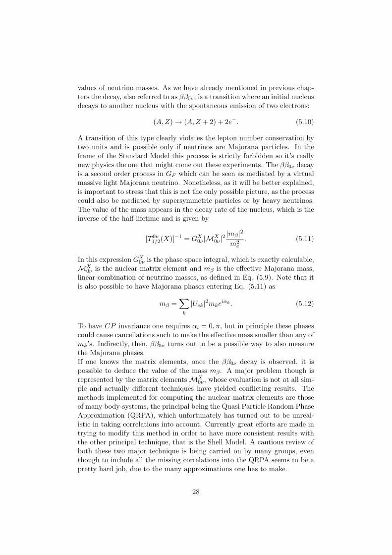
values of neutrino masses. As we have already mentioned in previous chap-ters the decay, also referred to as ββ0ν , is a transition where an initial nucleusdecays to another nucleus with the spontaneous emission of two electrons:

(A,Z)→ (A,Z + 2) + 2e−. (5.10)

A transition of this type clearly violates the lepton number conservation bytwo units and is possible only if neutrinos are Majorana particles. In theframe of the Standard Model this process is strictly forbidden so it’s reallynew physics the one that might come out these experiments. The ββ0ν decayis a second order process in GF which can be seen as mediated by a virtualmassive light Majorana neutrino. Nonetheless, as it will be better explained,is important to stress that this is not the only possible picture, as the processcould also be mediated by supersymmetric particles or by heavy neutrinos.The value of the mass appears in the decay rate of the nucleus, which is theinverse of the half-lifetime and is given by

[T 0ν1/2(X)]−1 = GX0ν |MX

0ν |2|mβ|2m2e

. (5.11)

In this expression GX0ν is the phase-space integral, which is exactly calculable,MX

0ν is the nuclear matrix element and mβ is the effective Majorana mass,linear combination of neutrino masses, as defined in Eq. (5.9). Note that itis also possible to have Majorana phases entering Eq. (5.11) as

mβ =∑

k

|Uek|2mkeiαk . (5.12)

To have CP invariance one requires αi = 0, π, but in principle these phasescould cause cancellations such to make the effective mass smaller than any ofmk’s. Indirectly, then, ββ0ν turns out to be a possible way to also measurethe Majorana phases.If one knows the matrix elements, once the ββ0ν decay is observed, it ispossible to deduce the value of the mass mβ . A major problem though isrepresented by the matrix elementsMX

0ν , whose evaluation is not at all sim-ple and actually different techniques have yielded conflicting results. Themethods implemented for computing the nuclear matrix elements are thoseof many body-systems, the principal being the Quasi Particle Random PhaseApproximation (QRPA), which unfortunately has turned out to be unreal-istic in taking correlations into account. Currently great efforts are made intrying to modify this method in order to have more consistent results withthe other principal technique, that is the Shell Model. A cautious review ofboth these two major technique is being carried on by many groups, eventhough to include all the missing correlations into the QRPA seems to be apretty hard job, due to the many approximations one has to make.

28

The picture with light neutrinos being the exchanging particles in the pro-cess is not the only possible one though. Frameworks with heavy particles(or heavy neutrinos) or supersymmetric particles exchange that still violatethe lepton charge conservation at high energy scales can reproduce the sameelectron spectrum as the one obtained with the exchange of the light Ma-jorana neutrino. Should these other mechanism also happen with, by nowunknown, non-negligible probability, then the possibility of extrapolating thelight neutrino mass from ββ0ν would be in real danger. More specifically,if we choose the lepton charge violating energy scale to be of the order of1012 eV and take mβ ∼ 0.1−0.5 eV , then the contributions to the decay am-plitude of heavy particle and light particle exchange are of the same order,meaning that both pictures are possible. Very naively, the decay amplitudesin both case are given by

AL ∼ G2F

mβ

k2, AH ∼ G2

F

M4W

Λ5(5.13)

being Λ the heavy mass energy scale at which the lepton charge conservationis violated and k the typical light neutrino (virtual) momentum. The ratiobetween the two, with the chosen energy scale, is ∼ O(1). If we go to higherenergy scales (like 3× 1012 eV ), then AL becomes dominant.So far there is no clear evidence of any ββ0ν observation, even though in2002 there was a claim for an observation of neutrinoless double beta decayof 76Ge with T 0ν

1/2 = 1.9+1.00−0.17×1025 years, which has been recently confirmed

[9]. This claim has been long criticized but still there is no evidence forruling it out completely, so new generation experiments are expected to givea substantial contribution to this issue. Hereafter we list the recent ββ0ν

results, with the mass limits deduced by the authors from the half-life times.All limits are at 90% level of confidence, unless otherwise indicated. We see

Isotope Half-life limit (y) mβ (meV)48Ca > 1.4× 1022 < 7200− 4470076Ge > 1.9× 1025 < 350 (H-M)76Ge > 1.6× 1025 < 330− 1350 (IGEX)82Se > 2.7× 1022 (68%) < 5000

100Mo > 5.5× 1022 < 2100116Cd > 1.7× 1023 < 1700128Te > 7.7× 1024 < 1100− 1500130Te > 5.5× 1023 < 370− 1700136Xe > 4.4× 1023 < 1800− 5200150Nd > 1.2× 1021 < 3000

that the most stringent bound is the one obtained in the Heidelberg-Moscow

29

76Ge experiment, comparable with the IGEX experiment result, also on 76Ge.

New generation experiments (CUORE and GERDA at the LNGS, Italy,or MAJORANA or Super-NEMO, this last one not started yet) have as theirprincipal goal that of improving sensitivity in order to probe the invertedhierarchy (IH) of neutrino masses (m ∼ 10−50meV ). Such a goal is howeverfar from the allowance of the current technology and so phased projects havebeen launched both in the USA and Europe. Also the claimed evidence forββ0ν signal in the Heidelberg-Moscow experiment is one of the first goals tobe achieved in short time.Many experiments are being carried out for the search of neutrinoless doublebeta decay with different experimental techniques and isotopes. This is offundamental importance for many reasons; first of all the observation of asignal may not be considered a real discovery without being confirmed byother experiments on different isotopes. Also the theoretical uncertainty onthe nuclear matrix elements requires different experiments to get a reliablevalue for the effective mass. Finally, from experiments on different isotopesone can have deeper insights on whether the light neutrino scheme is indeedtrue or not: in fact the relative matrix elements for different nuclei dependon the exchange mechanism.Huge strides have been made in the last ten years in developing advancedtechniques for the investigation of ββ0ν . It is very likely that this will bethe field where experimental confirmations on the theoretical frame we havebeen discussing will soon be made. A key point, as usual, is how muchgovernments will be keen on spending for very expensive experiments.

30

References

[1] S.M.Bilenky, S.T. Petcov, Rev. Mod. Phys. 59 (1987) 67.

[2] C.Giunti, Nucl.Phys.Proc.Suppl. 169: 309-320, 2007, hep-ph/0611125.

[3] S.M.Bilenky, Casta-Papiernicka 1999, High-energy physics 187-217,1999, hep-ph/0001311.

[4] M. Kobayashi and T. Maskawa, Prog.Theor. Phys. 49, 652 (1973).

[5] E.Majorana, Nuovo Cimento 14 (1937) 171.

[6] G.Altarelli, Nuovo Cimento 032C: 91-102, 2009.

[7] O.Cremonesi, J.Phys.Conf.Ser. 202: 012037, 2010.

[8] S.M.Bilenky, C.Giunti and W.Grimus, Prog.Part.Nucl.Phys. 43 (1999)1, hep-ph/9812360.

[9] Klapdor-Kleingrothaus, Phys.Scr. T 127 (2006) 40.

[10] G.L.Fogli, E.Lisi, A.Marrone, A.Palazzo and A.M.Rotunno,Phys.Rev.Lett. 101 (2008) 141801.

[11] T.Schwetz, M.Tortola and J.W.F.Valle, New J. Phys. 10 (2008) 113011.

[12] G.Altarelli and F.Feruglio ,Phys. Rept. 320 (1999) 295.

[13] W.E.Burcham and M.Jobes Nuclear and Particle Physics, John Wileyand Sons, New York 1995.

[14] B.Martin Nuclear and Particle Physics: An Introduction, John Wileyand Sons, 2009.

[15] Fermilab MINOS experiment sheds light on mystery of neutrino disap-pearence.

[16] F.Bohem and P.Vogel Physics of Massive Neutrinos, Cambridge Uni-versity Press, Cambridge 1987.

[17] S.M.Bilenky and B.Pontecorvo, Phys. Rep. 41, 225 (1978).

[18] S.Petcov, P.Vogel et al. Neutrinoless Double Beta Decay and DirectSearches for Neutrino Masses, hep-ph/0412300v1, 2004.

[19] H.Fritzsch Flavor Mixing, Neutrino Masses and Neutrino OscillationsarXiv:0902.2817v1, 2009.

[20] G.Altarelli and F.Feruglio, New J.Phys. 6 (2004) 106.

31

[21] G.Altarelli, F.Feruglio and Y.Lin, Nucl. Phys. B 775 (2007) 31.

[22] M.Trodden, Rev. Mod. Phys. 71, 1463 (1999).

[23] P. Minkowski, Phys. Rev. Lett. B67 (1977) 421.

[24] S.Weinberg, Phys. Rev. Lett. 43 (1979) 1566.

32