Radiative Transfer in the Earth Systemdust.ess.uci.edu/facts/rt/rt.pdf · CONTENTS iii Contents...
181
Online: http://dust.ess.uci.edu/facts Built: Thu 14 th Sept, 2017, 12:35 Radiative Transfer in the Earth System by Charlie Zender University of California, Irvine Department of Earth System Science [email protected] University of California Voice: (949) 891-2429 Irvine, CA 92697-3100 Fax: (949) 824-3256 Copyright © 1998–2017, Charles S. Zender Permission is granted to copy, distribute and/or modify this document under the terms of the GNU Free Documentation License, Version 1.3 or any later version published by the Free Software Foundation; with no Invariant Sections, no Front-Cover Texts, and no Back-Cover Texts. The license is available online at http://www.gnu.org/copyleft/fdl.html. Facts about FACTs: This document is part of the Freely Available Community Text (fact) project. facts are created, reviewed, and continuously maintained and updated by mem- bers of the international academic community communicating with eachother through a well-organized project website. facts are intended to standardize and disseminate our fun- damental knowledge of Earth System Sciences in a flexible, adaptive, distributed framework which can evolve to fit the changing needs and technology of the geosciences community. Currently available facts and their urls are listed in Table 1. Because of its international Table 1: Freely Available Community Texts Format URL Location Radiative Transfer in the Earth System DVI http://dust.ess.uci.edu/facts/rt/rt.dvi PDF http://dust.ess.uci.edu/facts/rt/rt.pdf Postscript http://dust.ess.uci.edu/facts/rt/rt.ps Particle Size Distributions: Theory and Application to Aerosols, Clouds, and Soils DVI http://dust.ess.uci.edu/facts/psd/psd.dvi PDF http://dust.ess.uci.edu/facts/psd/psd.pdf Postscript http://dust.ess.uci.edu/facts/psd/psd.ps Natural Aerosols in the Climate System DVI http://dust.ess.uci.edu/facts/aer/aer.dvi PDF http://dust.ess.uci.edu/facts/aer/aer.pdf Postscript http://dust.ess.uci.edu/facts/aer/aer.ps scope and availability to students of all income levels, the fact project may impact more students, and to a greater depth, than imaginable to before the advent of the Internet. If you are interested in learning more about facts and how you might contribute to or benefit from the project please contact [email protected].
Transcript of Radiative Transfer in the Earth Systemdust.ess.uci.edu/facts/rt/rt.pdf · CONTENTS iii Contents...
Online: http://dust.ess.uci.edu/facts Built: Thu 14th Sept, 2017, 12:35
Radiative Transfer in the Earth Systemby Charlie Zender
University of California, Irvine
Department of Earth System Science [email protected] of California Voice: (949) 891-2429Irvine, CA 92697-3100 Fax: (949) 824-3256
Copyright © 1998–2017, Charles S. ZenderPermission is granted to copy, distribute and/or modify this document under the terms ofthe GNU Free Documentation License, Version 1.3 or any later version published by the FreeSoftware Foundation; with no Invariant Sections, no Front-Cover Texts, and no Back-CoverTexts. The license is available online at http://www.gnu.org/copyleft/fdl.html.
Facts about FACTs: This document is part of the Freely Available Community Text (fact)project. facts are created, reviewed, and continuously maintained and updated by mem-bers of the international academic community communicating with eachother through awell-organized project website. facts are intended to standardize and disseminate our fun-damental knowledge of Earth System Sciences in a flexible, adaptive, distributed frameworkwhich can evolve to fit the changing needs and technology of the geosciences community.Currently available facts and their urls are listed in Table 1. Because of its international
Table 1: Freely Available Community TextsFormat URL Location
Radiative Transfer in the Earth SystemDVI http://dust.ess.uci.edu/facts/rt/rt.dviPDF http://dust.ess.uci.edu/facts/rt/rt.pdf
Postscript http://dust.ess.uci.edu/facts/rt/rt.psParticle Size Distributions: Theory and Application to Aerosols, Clouds, and Soils
DVI http://dust.ess.uci.edu/facts/psd/psd.dviPDF http://dust.ess.uci.edu/facts/psd/psd.pdf
Postscript http://dust.ess.uci.edu/facts/psd/psd.psNatural Aerosols in the Climate System
DVI http://dust.ess.uci.edu/facts/aer/aer.dviPDF http://dust.ess.uci.edu/facts/aer/aer.pdf
Postscript http://dust.ess.uci.edu/facts/aer/aer.ps
scope and availability to students of all income levels, the fact project may impact morestudents, and to a greater depth, than imaginable to before the advent of the Internet. Ifyou are interested in learning more about facts and how you might contribute to or benefitfrom the project please contact [email protected].

ii
Notes for Students of ESS 223,Earth System Physics:
This monograph on Radiative Transfer provides some core and some supplementary readingmaterial for ESS 223. We will discuss much of the material in the first twenty pages, andthe figures at the end. The Index beginning on page 171 is also helpful.
Notes for Students of ESS 236,Radiative Transfer and Remote Sensing:
Yada yada yada.

CONTENTS iii
Contents
Contents iii
List of Figures vi
List of Tables 1
1 Introduction 11.1 Planetary Radiative Equilibrium . . . . . . . . . . . . . . . . . . . . . . . . 11.2 Fundamentals . . . . . . . . . . . . . . . . . . . . . . . . . . . . . . . . . . . 2
2 Radiative Transfer Equation 42.1 Definitions . . . . . . . . . . . . . . . . . . . . . . . . . . . . . . . . . . . . . 4
2.1.1 Intensity . . . . . . . . . . . . . . . . . . . . . . . . . . . . . . . . . . 42.1.2 Mean Intensity . . . . . . . . . . . . . . . . . . . . . . . . . . . . . . 52.1.3 Irradiance . . . . . . . . . . . . . . . . . . . . . . . . . . . . . . . . . 72.1.4 Actinic Flux . . . . . . . . . . . . . . . . . . . . . . . . . . . . . . . . 82.1.5 Actinic Flux Enhancement . . . . . . . . . . . . . . . . . . . . . . . . 112.1.6 Energy Density . . . . . . . . . . . . . . . . . . . . . . . . . . . . . . 152.1.7 Spectral vs. Broadband . . . . . . . . . . . . . . . . . . . . . . . . . 152.1.8 Thermodynamic Equilibria . . . . . . . . . . . . . . . . . . . . . . . 162.1.9 Planck Function . . . . . . . . . . . . . . . . . . . . . . . . . . . . . 172.1.10 Hemispheric Quantities . . . . . . . . . . . . . . . . . . . . . . . . . 192.1.11 Stefan-Boltzmann Law . . . . . . . . . . . . . . . . . . . . . . . . . . 212.1.12 Luminosity . . . . . . . . . . . . . . . . . . . . . . . . . . . . . . . . 242.1.13 Extinction and Emission . . . . . . . . . . . . . . . . . . . . . . . . . 252.1.14 Optical Depth . . . . . . . . . . . . . . . . . . . . . . . . . . . . . . 262.1.15 Geometric Derivation of Optical Depth . . . . . . . . . . . . . . . . . 272.1.16 Stratified Atmosphere . . . . . . . . . . . . . . . . . . . . . . . . . . 29
2.2 Integral Equations . . . . . . . . . . . . . . . . . . . . . . . . . . . . . . . . 312.2.1 Formal Solutions . . . . . . . . . . . . . . . . . . . . . . . . . . . . . 312.2.2 Thermal Radiation In A Stratified Atmosphere . . . . . . . . . . . . 332.2.3 Angular Integration . . . . . . . . . . . . . . . . . . . . . . . . . . . 332.2.4 Thermal Irradiance . . . . . . . . . . . . . . . . . . . . . . . . . . . . 342.2.5 Grey Atmosphere . . . . . . . . . . . . . . . . . . . . . . . . . . . . . 352.2.6 Scattering . . . . . . . . . . . . . . . . . . . . . . . . . . . . . . . . . 392.2.7 Phase Function . . . . . . . . . . . . . . . . . . . . . . . . . . . . . . 402.2.8 Legendre Basis Functions . . . . . . . . . . . . . . . . . . . . . . . . 402.2.9 Henyey-Greenstein Approximation . . . . . . . . . . . . . . . . . . . 412.2.10 Direct and Diffuse Components . . . . . . . . . . . . . . . . . . . . . 422.2.11 Source Function . . . . . . . . . . . . . . . . . . . . . . . . . . . . . 432.2.12 Radiative Transfer Equation in Slab Geometry . . . . . . . . . . . . 442.2.13 Azimuthal Mean Radiation Field . . . . . . . . . . . . . . . . . . . . 452.2.14 Anisotropic Scattering . . . . . . . . . . . . . . . . . . . . . . . . . . 48
CONTENTS iv
2.2.15 Diffusivity Approximation . . . . . . . . . . . . . . . . . . . . . . . . 482.2.16 Transmittance . . . . . . . . . . . . . . . . . . . . . . . . . . . . . . 50
2.3 Reflection, Transmission, Absorption . . . . . . . . . . . . . . . . . . . . . . 512.3.1 BRDF . . . . . . . . . . . . . . . . . . . . . . . . . . . . . . . . . . . 522.3.2 Lambertian Surfaces . . . . . . . . . . . . . . . . . . . . . . . . . . . 522.3.3 Albedo . . . . . . . . . . . . . . . . . . . . . . . . . . . . . . . . . . 532.3.4 Flux Transmission . . . . . . . . . . . . . . . . . . . . . . . . . . . . 55
2.4 Two-Stream Approximation . . . . . . . . . . . . . . . . . . . . . . . . . . . 562.4.1 Two-Stream Equations . . . . . . . . . . . . . . . . . . . . . . . . . . 582.4.2 Layer Optical Properties . . . . . . . . . . . . . . . . . . . . . . . . . 612.4.3 Conservative Scattering Limit . . . . . . . . . . . . . . . . . . . . . . 61
2.5 Solar Heating . . . . . . . . . . . . . . . . . . . . . . . . . . . . . . . . . . . 632.6 Chapter Exercises . . . . . . . . . . . . . . . . . . . . . . . . . . . . . . . . . 63
3 Remote Sensing 643.1 Rayleigh Limit . . . . . . . . . . . . . . . . . . . . . . . . . . . . . . . . . . 643.2 Anomalous Diffraction Theory . . . . . . . . . . . . . . . . . . . . . . . . . . 653.3 Geometric Optics Approximation . . . . . . . . . . . . . . . . . . . . . . . . 683.4 Single Scattered Intensity . . . . . . . . . . . . . . . . . . . . . . . . . . . . 693.5 Satellite Orbits . . . . . . . . . . . . . . . . . . . . . . . . . . . . . . . . . . 693.6 Aerosol Characterization . . . . . . . . . . . . . . . . . . . . . . . . . . . . . 71
3.6.1 Measuring Aerosol Optical Depth . . . . . . . . . . . . . . . . . . . . 713.6.2 Aerosol Indirect Effects on Climate . . . . . . . . . . . . . . . . . . . 713.6.3 Aerosol Effects on Snow and Ice Albedo . . . . . . . . . . . . . . . . 713.6.4 Ångström Exponent . . . . . . . . . . . . . . . . . . . . . . . . . . . 72
4 Gaseous Absorption 724.1 Line Shape . . . . . . . . . . . . . . . . . . . . . . . . . . . . . . . . . . . . 72
4.1.1 Line Shape Factor . . . . . . . . . . . . . . . . . . . . . . . . . . . . 724.1.2 Natural Line Shape . . . . . . . . . . . . . . . . . . . . . . . . . . . . 744.1.3 Pressure Broadening . . . . . . . . . . . . . . . . . . . . . . . . . . . 764.1.4 Doppler Broadening . . . . . . . . . . . . . . . . . . . . . . . . . . . 814.1.5 Voigt Line Shape . . . . . . . . . . . . . . . . . . . . . . . . . . . . . 83
5 Molecular Absorption 845.1 Mechanical Analogues . . . . . . . . . . . . . . . . . . . . . . . . . . . . . . 84
5.1.1 Vibrational Transitions . . . . . . . . . . . . . . . . . . . . . . . . . . 875.1.2 Isotopic Lines . . . . . . . . . . . . . . . . . . . . . . . . . . . . . . . 895.1.3 Combination Bands . . . . . . . . . . . . . . . . . . . . . . . . . . . 89
5.2 Partition Functions . . . . . . . . . . . . . . . . . . . . . . . . . . . . . . . . 905.3 Dipole Radiation . . . . . . . . . . . . . . . . . . . . . . . . . . . . . . . . . 935.4 Two Level Atom . . . . . . . . . . . . . . . . . . . . . . . . . . . . . . . . . 935.5 Line Strengths . . . . . . . . . . . . . . . . . . . . . . . . . . . . . . . . . . 95
5.5.1 hitran . . . . . . . . . . . . . . . . . . . . . . . . . . . . . . . . . . . 955.6 Line-By-Line Models . . . . . . . . . . . . . . . . . . . . . . . . . . . . . . . 98

CONTENTS v
5.6.1 Literature . . . . . . . . . . . . . . . . . . . . . . . . . . . . . . . . . 98
6 Band Models 986.1 Generic . . . . . . . . . . . . . . . . . . . . . . . . . . . . . . . . . . . . . . 98
6.1.1 Beam Transmittance . . . . . . . . . . . . . . . . . . . . . . . . . . . 996.1.2 Beam Absorptance . . . . . . . . . . . . . . . . . . . . . . . . . . . . 1006.1.3 Equivalent Width . . . . . . . . . . . . . . . . . . . . . . . . . . . . . 1006.1.4 Mean Absorptance . . . . . . . . . . . . . . . . . . . . . . . . . . . . 101
6.2 Line Distributions . . . . . . . . . . . . . . . . . . . . . . . . . . . . . . . . 1046.2.1 Line Strength Distributions . . . . . . . . . . . . . . . . . . . . . . . 1046.2.2 Normalization . . . . . . . . . . . . . . . . . . . . . . . . . . . . . . . 1066.2.3 Mean Line Intensity . . . . . . . . . . . . . . . . . . . . . . . . . . . 1086.2.4 Mean Absorptance of Line Distribution . . . . . . . . . . . . . . . . . 1096.2.5 Transmittance . . . . . . . . . . . . . . . . . . . . . . . . . . . . . . 1186.2.6 Multiplication Property . . . . . . . . . . . . . . . . . . . . . . . . . 118
6.3 Transmission in Inhomogeneous Atmospheres . . . . . . . . . . . . . . . . . 1196.3.1 Constant mixing ratio . . . . . . . . . . . . . . . . . . . . . . . . . . 1196.3.2 H-C-G Approximation . . . . . . . . . . . . . . . . . . . . . . . . . . 120
6.4 Temperature Dependence . . . . . . . . . . . . . . . . . . . . . . . . . . . . 1226.5 Transmission in Spherical Atmospheres . . . . . . . . . . . . . . . . . . . . . 123
6.5.1 Chapman Function . . . . . . . . . . . . . . . . . . . . . . . . . . . . 123
7 Radiative Effects of Aerosols and Clouds 1247.1 Single Scattering Properties . . . . . . . . . . . . . . . . . . . . . . . . . . . 124
7.1.1 Maxwell Equations . . . . . . . . . . . . . . . . . . . . . . . . . . . . 1257.2 Separation of Variables . . . . . . . . . . . . . . . . . . . . . . . . . . . . . . 129
7.2.1 Azimuthal Solutions . . . . . . . . . . . . . . . . . . . . . . . . . . . 1297.2.2 Polar Solutions . . . . . . . . . . . . . . . . . . . . . . . . . . . . . . 1307.2.3 Radial Solutions . . . . . . . . . . . . . . . . . . . . . . . . . . . . . 1317.2.4 Plane Wave Expansion . . . . . . . . . . . . . . . . . . . . . . . . . . 1337.2.5 Boundary Conditions . . . . . . . . . . . . . . . . . . . . . . . . . . . 1347.2.6 Mie Theory . . . . . . . . . . . . . . . . . . . . . . . . . . . . . . . . 1347.2.7 Resonances . . . . . . . . . . . . . . . . . . . . . . . . . . . . . . . . 1357.2.8 Optical Efficiencies . . . . . . . . . . . . . . . . . . . . . . . . . . . . 1367.2.9 Optical Cross Sections . . . . . . . . . . . . . . . . . . . . . . . . . . 1377.2.10 Optical Depths . . . . . . . . . . . . . . . . . . . . . . . . . . . . . . 1377.2.11 Single Scattering Albedo . . . . . . . . . . . . . . . . . . . . . . . . . 1377.2.12 Asymmetry Parameter . . . . . . . . . . . . . . . . . . . . . . . . . . 1377.2.13 Mass Absorption Coefficient . . . . . . . . . . . . . . . . . . . . . . . 138
7.3 Effective Single Scattering Properties . . . . . . . . . . . . . . . . . . . . . . 1387.3.1 Effective Efficiencies . . . . . . . . . . . . . . . . . . . . . . . . . . . 1387.3.2 Effective Cross Sections . . . . . . . . . . . . . . . . . . . . . . . . . 1397.3.3 Effective Specific Extinction Coefficients . . . . . . . . . . . . . . . . 1397.3.4 Effective Optical Depths . . . . . . . . . . . . . . . . . . . . . . . . . 1397.3.5 Effective Single Scattering Albedo . . . . . . . . . . . . . . . . . . . 139

LIST OF FIGURES vi
7.3.6 Effective Asymmetry Parameter . . . . . . . . . . . . . . . . . . . . . 1407.4 Mean Effective Single Scattering Properties . . . . . . . . . . . . . . . . . . 140
7.4.1 Mean Effective Efficiencies . . . . . . . . . . . . . . . . . . . . . . . . 1417.4.2 Mean Effective Cross Sections . . . . . . . . . . . . . . . . . . . . . . 1417.4.3 Mean Effective Specific Extinction Coefficients . . . . . . . . . . . . . 1417.4.4 Mean Effective Optical Depths . . . . . . . . . . . . . . . . . . . . . 1427.4.5 Mean Effective Single Scattering Albedo . . . . . . . . . . . . . . . . 1427.4.6 Mean Effective Asymmetry Parameter . . . . . . . . . . . . . . . . . 142
7.5 Bulk Layer Single Scattering Properties . . . . . . . . . . . . . . . . . . . . . 1427.5.1 Addition of Optical Properties . . . . . . . . . . . . . . . . . . . . . 1427.5.2 Bulk Optical Depths . . . . . . . . . . . . . . . . . . . . . . . . . . . 1437.5.3 Bulk Single Scattering Albedo . . . . . . . . . . . . . . . . . . . . . . 1437.5.4 Bulk Asymmetry Parameter . . . . . . . . . . . . . . . . . . . . . . . 1437.5.5 Diagnostics . . . . . . . . . . . . . . . . . . . . . . . . . . . . . . . . 143
8 Global Radiative Forcing 143
9 Implementation in NCAR models 148
10 Appendix 15410.1 Vector Identities . . . . . . . . . . . . . . . . . . . . . . . . . . . . . . . . . 15410.2 Legendre Polynomials . . . . . . . . . . . . . . . . . . . . . . . . . . . . . . 15610.3 Spherical Harmonics . . . . . . . . . . . . . . . . . . . . . . . . . . . . . . . 15610.4 Bessel Functions . . . . . . . . . . . . . . . . . . . . . . . . . . . . . . . . . 157
10.4.1 Spherical Bessel Functions . . . . . . . . . . . . . . . . . . . . . . . . 15810.4.2 Recurrence Relations . . . . . . . . . . . . . . . . . . . . . . . . . . . 15810.4.3 Power Series Representation . . . . . . . . . . . . . . . . . . . . . . . 15810.4.4 Asymptotic Values . . . . . . . . . . . . . . . . . . . . . . . . . . . . 159
10.5 Gaussian Quadrature . . . . . . . . . . . . . . . . . . . . . . . . . . . . . . . 15910.6 Gauss-Lobatto Quadrature . . . . . . . . . . . . . . . . . . . . . . . . . . . . 16210.7 Exponential Integrals . . . . . . . . . . . . . . . . . . . . . . . . . . . . . . . 163
Bibliography 164
Index 171
List of Figures1 Cross Section and Quantum Yield of Nitrogen Dioxide . . . . . . . . . . . . 122 Vertical Distribution of Photodissociation Rates . . . . . . . . . . . . . . . . 133 Climatological Mean Absorbed Solar Radiation . . . . . . . . . . . . . . . . 1444 Climatological Mean Emitted Longwave Radiation . . . . . . . . . . . . . . 1455 ENSO Temperature and OLR . . . . . . . . . . . . . . . . . . . . . . . . . . 1466 Seasonal Shortwave Cloud Forcing . . . . . . . . . . . . . . . . . . . . . . . 1477 Zonal Mean Shortwave Cloud Forcing . . . . . . . . . . . . . . . . . . . . . . 149

8 Seasonal Longwave Cloud Forcing . . . . . . . . . . . . . . . . . . . . . . . . 1509 Zonal Mean Longwave Cloud Forcing . . . . . . . . . . . . . . . . . . . . . . 15110 Climatological Mean Net Cloud Forcing . . . . . . . . . . . . . . . . . . . . 15211 ENSO Cloud Forcing . . . . . . . . . . . . . . . . . . . . . . . . . . . . . . . 153
List of Tables1 facts . . . . . . . . . . . . . . . . . . . . . . . . . . . . . . . . . . . . . . . . i2 Wave Parameter Conversion Table . . . . . . . . . . . . . . . . . . . . . . . 43 Actinic Flux Enhancement . . . . . . . . . . . . . . . . . . . . . . . . . . . . 114 Surface Albedo . . . . . . . . . . . . . . . . . . . . . . . . . . . . . . . . . . 545 Temperature Dependence of αp . . . . . . . . . . . . . . . . . . . . . . . . . 796 Pressure-Broadened Half Widths . . . . . . . . . . . . . . . . . . . . . . . . 807 Mechanical Analogues of Important Gases . . . . . . . . . . . . . . . . . . . 878 hitran database . . . . . . . . . . . . . . . . . . . . . . . . . . . . . . . . . . 959 Full-range Gaussian quadrature . . . . . . . . . . . . . . . . . . . . . . . . . 16110 Half-range Gaussian quadrature . . . . . . . . . . . . . . . . . . . . . . . . . 161
1 IntroductionThis document describes mathematical and computational considerations pertaining to ra-diative transfer processes and radiative transfer models of the Earth system. Our approachis to present a detailed derivation of the tools of radiative transfer needed to predict theradiative quantities (irradiance, mean intensity, and heating rates) which drive climate. Inso doing we begin with discussion of the intensity field which is the quantity most oftenmeasured by satellite remote sensing instruments. Our approach owes much to Bohren andHuffman (1983) (particle scattering), Goody and Yung (1989) (band models), and Thomasand Stamnes (1999) (nomenclature, discrete ordinate methods, general approach). Thenomenclature follows these authors where possible. These sections will evolve and differen-tiate from their original sources as the manuscript takes on the flavor of the researchers whocontribute to it.
1.1 Planetary Radiative EquilibriumThe important role that radiation plays in the climate system is perhaps best illustrated by asimple example showing that without atmospheric radiative feedbacks (especially, ironically,the greenhouse effect), our planet’s mean temperature would be well below the freezing pointof water. Earth is surrounded by the near vacuum of space so the only way to transportenergy to or from the planet is via radiative processes. If E is the thermal energy of theplanet, and FASR and FOLR are the absorbed solar radiation and emitted longwave radiation,respectively, then
∂E
∂t= FASR − FOLR (1)

1 INTRODUCTION 2
On timescales longer than about a year the Earth as a whole is thought to be in planetaryradiative equilibrium. That, is, the global annual mean planetary temperature is nearlyconstant because the absorbed solar energy is exactly compensated by thermal radiationlost to space over the course of a year. Thus
FASR = FOLR (2)
The total amount of solar energy available for the Earth to absorb is the incoming solarflux (or irradiance) at the top of Earth’s atmosphere, F (aka the solar constant), times theintercepting area of Earth’s disk which is πr2⊕. Since Earth rotates, the total mean incidentflux πr2⊕F is actually distributed over the entire surface area of the Earth. The surfacearea of a sphere is four times its cross-sectional area so the mean incident flux per unitsurface area is F/4. The fraction of incident solar flux which is reflected back to space,and thus unable to heat the planet, is called the aplanetary albedo or spherical albedo, R.Satellite observations show that R ≈ 0.3. Thus only (1−R) of the mean incident solar fluxcontributes to warming the planet and we have
FASR = (1−R)F/4 (3)
Earth does not cool to space as a perfect blackbody (41a) of a single temperature andemissivity. Nevertheless the spectrum of thermal radiation FOLR which escapes to spaceand thus cools Earth does resemble blackbody emission with a characteristic temperature.The effective temperature TE of an object is the temperature of the blackbody which wouldproduce the same irradiance. Inverting the Stefan-Boltzmann Law (73) yields
TE ≡ (FOLR/σ)1/4 (4)
For a perfect blackbody, T = TE. For a planet, the difference between TE and the meansurface temperature Ts is due to the radiative effects of the overlying atmosphere. Theinsulating behavior of the atmosphere is more commonly known as the greenhouse effect.
Substituting (3) and (4) into (2)
(1−R)F/4 = σT 4E (5)
TE =
((1−R)F
4σ
)1/4
(6)
For Earth, R ≈ 0.3 and F ≈ 1367W m−2. Using these values in (6) yields TE = 255K.Observations show the mean surface temperature Ts = 288K.
1.2 FundamentalsThe fundamental quantity describing the electromagnetic spectrum is frequency, ν. Fre-quency measures the oscillatory speed of a system, counting the number of oscillations(waves) per unit time. Usually ν is expressed in cycles-per-second, or Hertz. Units ofHertz may be abbreviated Hz, hz, cps, or, as we prefer, s−1. Frequency is intrinsic to the

1 INTRODUCTION 3
oscillator and does not depend on the medium in which the waves are travelling. The energycarried by a photon is proportional to its frequency
E = hν (7)
where h is Planck’s constant. Regrettably, almost no radiative transfer literature expressesquantities in frequency.
A related quantity, the angular frequency ω measures the rate of change of wave phasein radians per second. Wave phase proceeds through 2π radians in a complete cycle. Thusthe frequency and angular frequency are simply related
ω = 2πν (8)
Since radians are considered dimensionless, the units of ω are s−1. However, angular fre-quency is also rarely used in radiative transfer. Thus some authors use the symbol ω todenote the element of solid angle, as in dω. The reader should be careful not to misconstruethe two meanings. In this text we use ω only infrequently.
Most radiative transfer literature use wavelength or wavenumber. Wavelength, λ (m),measures the distance between two adjacent peaks or troughs in the wavefield. The universalrelation between wavelength and frequency is
λν = c (9)
where c is the speed of light. Since c depends on the medium, λ also depends on the medium.The wavenumber ν m−1, is exactly the inverse of wavelength
ν ≡ 1
λ=ν
c(10)
Thus ν measures the number of oscillations per unit distance, i.e., the number of wavecrestsper meter. Using (9) in (10) we find ν = ν/c so wavenumber ν is indeed proportional tofrequency (and thus to energy). Historically spectroscopists have favored ν rather than λor ν. Because of this history, it is much more common in the literature to find ν expressedin CGS units of cm−1 than in SI units of m−1. The CGS wavenumber is used analogouslyto frequency and to wavelength, i.e., to identify spectral regions. The energy of radiativetransitions are commonly expressed in CGS wavenumber units. The relation between νexpressed in CGS wavenumber units (cm−1) and energy in SI units (J) is obtained by using(10) in (7)
E = 100hcν (11)
There is another, distinct quantity also called wavenumber. This secondary usage ofwavenumber in this text is the traditional measure of spatial wave propagation and is denotedby k.
k ≡ 2πν (12)
The wavenumber k is set in Roman typeface as an additional distinction between it andother symbols 1.
Table 2 summarizes the relationships between the fundamental parameters which describewave-like phenomena.
1The script k is already used for Boltzmann’s constant, absorption coefficients, and vibrational modes

2 RADIATIVE TRANSFER EQUATION 4
Table 2: Wave Parameter Conversion Tableab
Variable ν λ ν ω k τUnits s−1 m cm−1 s−1 m−1 s
ν − c
ν
ν
100c2πν
2πν
c
1
ν
λc
λ− 1
100λ
2πc
λ
2π
λ
λ
c
ν 100cν1
100ν− ν
200πc200πν
1
100cν
ωω
2π
2πc
ω
ω
200πc− ω
c
2π
ω
kkc
2π
2π
k
k
200πck − 2π
ck
τ1
τcτ
1
100cτ
2π
τ
2π
cτ−
aThe speed of light is c = 2.99792458× 10⁸ m s−1.bTable entries express the column in terms of the row.
2 Radiative Transfer Equation
2.1 Definitions2.1.1 Intensity
The fundamental quantity defining the radiation field is the specific intensity of radiation.Specific intensity, also known as radiance, measures the flux of radiant energy transportedin a given direction per unit cross sectional area orthogonal to the beam per unit time perunit solid angle per unit frequency (or wavelength, or wavenumber). The units of Iλ areJoule meter−2 second−1 steradian−1 meter−1. In SI dimensional notation, the units condenseto J m−2 s−1 sr−1 m−1. The SI unit of power (1 Watt ≡ 1 Joule per second) is preferred,leading to units of W m−2 sr−1 m−1. Often the specific intensity is expressed in terms ofspectral frequency Iν with units W m−2 sr−1 Hz−1 or spectral wavenumber (also Iν) withunits W m−2 sr−1 (cm−1)−1.
Consider light travelling in the direction Ω through the point r. Construct an infinitesi-mal element of surface area dS intersecting r and orthogonal to Ω. The radiant energy dEcrossing dS in time dt in the solid angle dΩ in the frequency range [ν, ν + dν] is related toIν(r, Ω) by
dE = Iν(r, Ω, t, ν) dS dt dΩdν (13)
It is not convenient to measure the radiant flux across surface orthogonal to Ω, as in (13),when we consider properties of radiation fields with preferred directions. If instead, we

2 RADIATIVE TRANSFER EQUATION 5
measure the intensity orthogonal to an arbitrarily oriented surface element dA with surfacenormal n, then we must alter (13) to account for projection of dS onto dA. If the anglebetween n and Ω is θ then
cos θ = n · Ω (14)and the projection of dS onto dA yields
dA = cos θ dS (15)
so thatdE = Iν(r, Ω, t, ν) cos θ dA dt dΩdν (16)
The conceptual advantage that (16) has over (13) is that (16) builds in the geometric factorrequired to convert to any preferred coordinate system defined by dA and its normal n. Inpractice dA is often chosen to be the local horizon.
The radiation field is a seven-dimensional quantity, depending upon three coordinatesin space, one in time, two in angle, and one in frequency. We shall usually indicate thedependence of spectral radiance and irradiance on frequency by using ν as a subscript, as inIν , in favor of the more explicit, but lengthier, notation I(ν). Three of the dimensions aresuperfluous to climate models and will be discarded: The time dependence of Iν is a functionof the atmospheric state and solar zenith angle and will only be discussed further in thoseterms, so we shall drop the explicitly dependence on t. We reduce the number of spatialdimensions from three to one by assuming a stratified atmosphere which is horizontallyhomogeneous and in which physical quantities may vary only in the vertical dimension z.Thus we replace r by z. This approximation is also known as a plane-parallel atmosphere,and comes with at least two important caveats: The first is the neglect of horizontal photontransport which can be important in inhomogeneous cloud and surface environments. Thesecond is the neglect of path length effects at large solar zenith angles which can dramaticallyaffect the mean intensity of the radiation field, and thus the atmospheric photochemistry.
With these assumptions, the intensity is a function only of vertical position and of di-rection, Iν(z, Ω). Often the optical depth τ (defined below), which increases monotonicallywith z, is used for the vertical coordinate instead of z. The angular direction of the radiationis specified in terms of the polar angle θ and the azithumal angle φ. The polar angle θ is theangle between Ω and the normal surface n that defines the coordinate system. The specificintensity of radiation traveling at polar angle θ and azimuthal angle φ at optical depth levelτ in a plane parallel atmosphere is denoted by Iν(τ, θ, φ). Specific intensity is also referredto as intensity.
Further simplification of the intensity field is possible if it meets certain criteria. If Iνis not a function of position (τ), then the field is homogeneous. If Iν is not a function ofdirection (Ω), then the field is isotropic.
2.1.2 Mean Intensity
The mean intensity is an integrated measure of the radiation field at any point r. Meanintensity Iν is defined as the mean value of the intensity field integrated over all angles.
Iν =
∫ΩIν dΩ∫ΩdΩ
(17)
2 RADIATIVE TRANSFER EQUATION 6
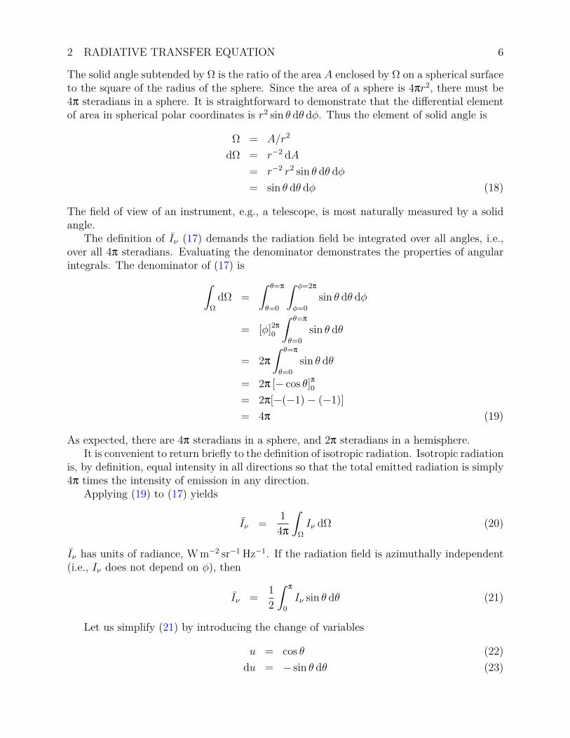
The solid angle subtended by Ω is the ratio of the area A enclosed by Ω on a spherical surfaceto the square of the radius of the sphere. Since the area of a sphere is 4πr2, there must be4π steradians in a sphere. It is straightforward to demonstrate that the differential elementof area in spherical polar coordinates is r2 sin θ dθ dφ. Thus the element of solid angle is
Ω = A/r2
dΩ = r−2 dA
= r−2 r2 sin θ dθ dφ
= sin θ dθ dφ (18)
The field of view of an instrument, e.g., a telescope, is most naturally measured by a solidangle.
The definition of Iν (17) demands the radiation field be integrated over all angles, i.e.,over all 4π steradians. Evaluating the denominator demonstrates the properties of angularintegrals. The denominator of (17) is∫
Ω
dΩ =
∫ θ=π
θ=0
∫ φ=2π
φ=0
sin θ dθ dφ
= [φ]2π
0
∫ θ=π
θ=0
sin θ dθ
= 2π
∫ θ=π
θ=0
sin θ dθ
= 2π [− cos θ]π0= 2π[−(−1)− (−1)]= 4π (19)
As expected, there are 4π steradians in a sphere, and 2π steradians in a hemisphere.It is convenient to return briefly to the definition of isotropic radiation. Isotropic radiation
is, by definition, equal intensity in all directions so that the total emitted radiation is simply4π times the intensity of emission in any direction.
Applying (19) to (17) yields
Iν =1
4π
∫Ω
Iν dΩ (20)
Iν has units of radiance, W m−2 sr−1 Hz−1. If the radiation field is azimuthally independent(i.e., Iν does not depend on φ), then
Iν =1
2
∫π
0
Iν sin θ dθ (21)
Let us simplify (21) by introducing the change of variables
u = cos θ (22)du = − sin θ dθ (23)

2 RADIATIVE TRANSFER EQUATION 7
This maps θ ∈ [0, π] into u ∈ [1,−1] so that (21) becomes
Iν = −1
2
∫ −1
1
Iν du
Iν =1
2
∫ 1
−1
Iν du (24)
The hemispheric intensities or half-range intensities are simply the up- and downwellingcomponents of which the full intensity is composed
Iν(τ, Ω) = Iν(τ, θ, φ) =
I+ν (τ, θ, φ) : 0 < θ < π/2I−ν (τ, θ, φ) : π/2 < θ < π
(25a)
Iν(τ, Ω) = Iν(τ, u, φ) =
I+ν (τ, u, φ) : 0 ≤ u < 1I−ν (τ, u, φ) : −1 < u < 0
(25b)
I+ν (τ, µ, φ) = Iν(τ,+µ, φ) = Iν(τ, 0 < θ < π/2, φ) = Iν(τ, 0 < u < 1, φ) (26a)I−ν (τ, µ, φ) = Iν(τ,+µ, φ) = Iν(τ, π/2 < θ < π, φ) = Iν(τ,−1 < u < 0, φ) (26b)
2.1.3 Irradiance
The spectral irradiance Fν measures the radiant energy flux transported through a givensurface per unit area per unit time per unit wavelength. Although it is somewhat ambiguous,“flux” is used a synonym for irradiance, and has become deeply embedded in the literature(Madronich, 1987). Consider a surface orthogonal to the Ω′ direction. All radiant energytravelling parallel to Ω′ crosses this surface and thus contributes to the irradiance with 100%efficiency. Energy travelling orthogonal to Ω′ (and thus parallel to the surface), however,never crosses the surface and does not contribute to the irradiance. In general, the intensityIν(Ω) projects onto the surface with an efficiency cosΘ = Ω · Ω′, thus
Fν =
∫Ω
Iν cos θ dΩ
=
∫ θ=π
θ=0
∫ φ=2π
φ=0
Iν cos θ sin θ dθ dφ (27)
In a plane-parallel medium, this defines the net specific irradiance passing through a givenvertical level. Note the similarity between (20) and (27). The former contains the zerothmoment of the intensity with respect to the cosine of the polar angle, the latter contains thefirst moment. Also note that (27) integrates the cosine-weighted radiance over all angles. IfIν is isotropic, i.e., Iν = I0ν , then Fν = 0 due to the symmetry of cos θ.
Let us simplify (27) by introducing the change of variables u = cos θ, du = − sin θ dθ.This maps θ ∈ [0, π] into u ∈ [1,−1]:
Fν =
∫ u=−1
u=1
∫ φ=2π
φ=0
Iνu (−du) dφ
=
∫ u=1
u=−1
∫ φ=2π
φ=0
Iνu du dφ (28)

2 RADIATIVE TRANSFER EQUATION 8
The irradiance per unit frequency, Fν , is simply related to the irradiance per unit wave-length, Fλ. The total irradiance over any given frequency range, [ν, ν + dν], say, is Fν dν.The irradiance over the same physical range when expressed in wavelength, [λ, λ− dλ], say,is Fλ dλ. The negative sign is introduced since −dλ increases in the same direction as +dν.Equating the total irradiance over the same region of frequency/wavelength, we obtain
Fν dν = −Fλ dλ
Fν = −Fλdλ
dν
= −Fλd
dν
( cν
)= −Fλ
(− c
ν2
)Fν =
c
ν2Fλ =
λ2
cFλ (29)
Fλ =c
λ2Fν =
ν2
cFν (30)
Thus Fν and Fλ are always of the same sign.
2.1.4 Actinic Flux
A quantity of great importance in photochemistry is the total convergence of radiation ata point. This quantity, called the actinic flux, F J , determines the availability of photonsfor photochemical reactions. By definition, the intensity passing through a point P in thedirection Ω within the solid angle dΩ is Iν dΩ. We have not multiplied by cos θ since we areinterested in the energy passing along Ω (i.e., θ = 0). The energy from all directions passingthrough P is thus
F Jν =
∫4π
Iν dΩ
= 4πIν (31)
Thus the actinic flux is simply 4π times the mean intensity Iν (20). F Jν has units of
W m−2 Hz−1 which are identical to the units of irradiance Fν (27). Although the nomen-clature “actinic flux” is somewhat appropriate, it is also somewhat ambiguous. The “flux”measured by F J
ν at a point P is the energy convergence (per unit time, frequency, and area)through the surface of the sphere containing P . This differs from the “flux” measured by Fν ,which is the net energy transport (per unit time, frequency, and area) through a definedhorizontal surface. Thus it is safest to use the terms “actinic radiation field” for F J
ν and“irradiance” for Fν . Unfortunately the literature is permeated with the ambiguous terms“actinic flux” and “flux”, respectively.
The usefulness of actinic flux F Jν becomes apparent only in conjunction with additional,
species-dependent data describing the probability of photon absorption, or photo-absorption.Photo-absorption is the process of molecules absorbing photons. Each absorption removesenergy (a photon) from the actinic radiation field. The amount of photo-absorption per
2 RADIATIVE TRANSFER EQUATION 9
unit volume is proportional to the number concentration of the absorbing species NA [m−3],the actinic radiation field F J
ν , and the efficiency with with each molecule absorbs photons.This efficiency is called the absorption cross-section, molecular cross section, or simply cross-section. The absorption cross-section is denoted by α and has units of [m−2]. In the literature,however, values of α usually appear in CGS units [cm−2]. To make explicit the frequency-dependence of α we write α(ν). If α depends significantly on temperature, too (as is truefor ozone), we must consider α(ν, T ).
The probability, per unit time, per unit frequency that a single molecule of species A willabsorb a photon with frequency in [ν, ν + dν] is proportional to F J
ν (ν)α(ν)2. Thus α(ν) is
the effective cross-sectional area of a molecule for absorption. The absorption cross-sectionis the ratio between the number of photons (or total energy) absorbed by a molecule to thenumber (or total energy) per unit area convergent on the molecule. Let Fα
ν [W m−3] be theenergy absorbed per unit time, per unit frequency, per unit volume of air. Then
Fαν (ν) = NAF
Jν (ν)α(ν) (32)
where NA m−3 is the number concentration of A.Photochemists are interested in the probability of absorbed radiation severing molecular
bonds, and thus decomposing species AB into constituent species A and B. Notationallythis process may be written in any of the equivalent forms
AB + hν −→ A+ B
AB + hνν>ν0−→ A+ B
AB + hνλ<λ0−→ A+ B (33)
Both forms indicate that the efficiency with which reaction (33) proceeds is a function ofphoton energy hν. The second form makes explicit that the photodissociation reaction doesnot proceed unless ν < ν0, where ν0 is the photolysis cutoff frequency. In any case, photonenergy is conventionally written hν, rather than the less convenient hc/λ.
The probability that a photon absorbed by AB will result in the photodissociation ofAB, and the completion of (33), is called the quantum yield or quantum efficiency and isrepresented by φ. The probability φ is dimensionless3. In addition to its dependence onν, φ depends on temperature T for some important atmospheric reactions (such as ozonephotolysis). We explicitly annotate the T -dependence of φ only for pertinent reactions.Measurement of φ(ν) for all conditions and reactions of atmospheric interest is an ongoingand important laboratory task.
The specific photolysis rate coefficient for the photodissociation of a species A is thenumber of photodissociations of A occuring per unit time, per unit volume of air, per unitfrequency, per molecule of A. In accord with convention we denote the specific photolysis
2The proportionality constant is (hν)−1, i.e., when the actinic radiation field F Jν (ν) is converted from
energy (J m−2 s−1 Hz−1) to photons (# m−2 s−1 Hz−1) then F Jν (ν)α(ν) is the probability of absorption per
second per unit frequency3Azimuthal angle and quantum yield are both dimensionless quantities denoted by φ. The meaning of φ
should be clear from the context.
2 RADIATIVE TRANSFER EQUATION 10
rate coefficient by Jν . The units of Jν are s−1 Hz−1.
Jν =F Jν (ν)α(ν)φ(ν)
hν
=4πIν(ν)α(ν)φ(ν)
hν(34)
The photon energy in the denominator converts the energy per unit area in F Jν to units of
photons per unit area. The factor of α turns this photon flux into a photo-absorption rate perunit area. The final factor, φ, converts the photo-absorption rate into a photodissociationrate coefficient. Note that each factor in the numerator of (34) requires detailed spectralknowledge, either of the radiation field or of the photochemical behavior of the molecule inquestion. This complexity is a hallmark of atmospheric photochemistry.
The total photolysis rate coefficient J is obtained by integrating (34) over all frequenciesthat may contribute to photodissociation
J =
∫ν>ν0
Jν(ν) dν
=
∫ν>ν0
F Jν (ν)α(ν)φ(ν)
hνdν
=4π
h
∫ν>ν0
Iν(ν)α(ν)φ(ν)
νdν (35)
As mentioned above, evaluation of (35) requires essentially a complete knowledge of theradiative and photochemical properties of the environment and species of interest.
J is notoriously sensitive to uncertainty in the input quantities. Integration errors due tothe discretization of (35) are quite common. To compute J with high accuracy, regular gridsmust have resolution of ∼1 nm in the ultraviolet, (Madronich, 1989). Much of the difficultyis due to the steep but opposite gradients of F J
ν and φ that occur in the ultraviolet. Highfrequency features in α worsen this problem for some molecules.
The utility of J has motivated researchers to overcome these computational difficul-ties by brute force techniques and by clever parameterizations and numerical techniques(Chang et al., 1987; Dahlback and Stamnes, 1991; Toon et al., 1989; Stamnes and Tsay,1990; Petropavlovskikh, 1995; Landgraf and Crutzen, 1998; Wild et al., 2000). It is commonto refer to photolysis rate coeffients as “J-rates”, and to affix the name of the molecule tospecify which individual reaction is pertinent. Another description for J is the first order ratecoefficient in photochemical reactions. For example, JNO2 is the first order rate coefficientfor
NO2 + hνλ<420 nm−→ NO+O (36)
If [NO2] denotes the number concentration of NO2 in a closed system where photolysis is theonly sink of NO2, then
d[NO2]
dt= −JNO2 [NO2] + SNO2 (37)

2 RADIATIVE TRANSFER EQUATION 11
Table 3: Actinic Flux Enhancement by Scatteringa
Description F−ν ρL(ν) Iν(Ω) F+
ν Iν F Jν
Collimated,non-reflecting
Fν 0 F
ν δ(Ω− Ω) 0Fν
4πFν
Isotropic,non-reflecting
Fν 0
I−ν = Fν /π
I+ν = 00
Fν
2π2F
ν
Collimated,reflecting
Fν 1
I−ν = Fν δ(Ω− Ω)
I+ν = Fν /π
Fν
3Fν
4π3F
ν
Isotropic,reflecting
Fν 1 F
ν /π Fν
Fν
π4F
ν
aTerminology: F−ν is downwelling irradiance of source, ρL(ν) is Lambertian reflectance of surface (or
cloud), Iν(Ω) is resulting intensity field, F+ν is upwelling irradiance, Iν is mean intensity, F J
ν is actinic flux.
where SNO2 represents all sources of NO2. The terms in (37) all have dimensions of m−3 s−1.The first term on the RHS is the photolysis rate of NO2 in the system.
Figure 1 shows the spectral distribution of actinic flux in a clear mid-latitude summeratmosphere, and the absorption cross-section and quantum yield of NO2.
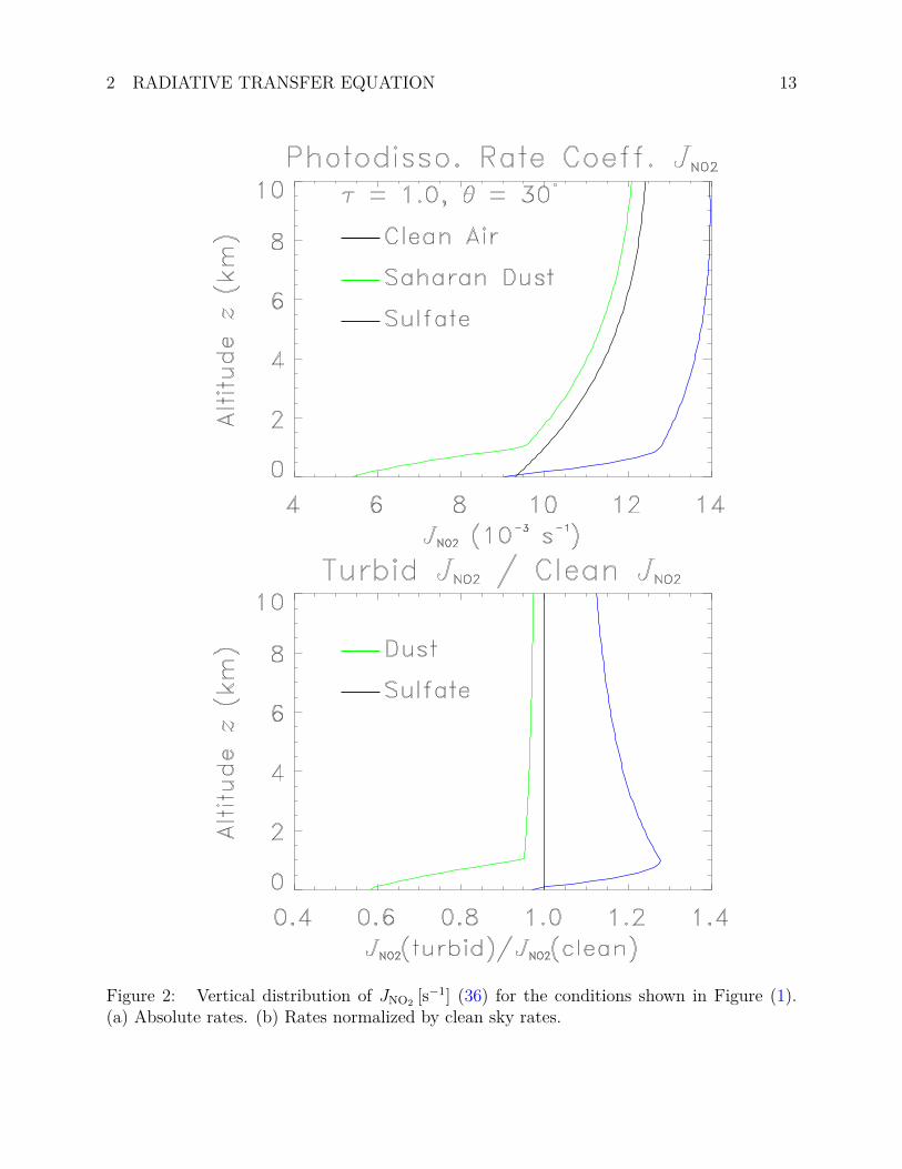
Figure 2 shows the vertical distribution of JNO2 [s−1] for the conditions shown in Fig-ure (1).
In this section we have assumed the quantities F Jν , α, and φ are somehow known and
therefore available to use to compute J . Typically, α and φ are considered known quantitiessince they usually do not vary with time or space. Models may store their values in lookuptables or precompute their contributions to (35). The essence of forward radiative problemsis to determine Iν so that quantities such as Jν and Fα may be determined. In inverseradiative transfer problems, which are encountered in much of remote sensing, both J andthe species concentration are initially unknown and must be determined. We shall continuedescribing the methods of forward radiative transfer until we have tools at our disposal tosolve for Jν . At that point we shall re-visit the inverse problem.
2.1.5 Actinic Flux Enhancement
The actinic flux F Jν (31) is sensitive to the angular distribution of radiance Iν . Nearly
all scattering processes diffuse the radiation field, i.e., convert collimated photons to moreisotropic photons. Such diffusion causes actinic flux enhancement. It is instructive to exam-ine how the relationship between downwelling flux and actinic flux changes in the presenceof scattering. Four limiting cases may be identified and are summarized in Table 3. Thescenarios differ in the isotropicity of the downwelling radiance (collimated or isotropic) andthe reflectance ρL(ν) (0 or 1) of the lower boundary, taken to be a Lambertian surface. Allscenarios are driven by the same downwelling irradiance, taken to be the direct solar beam.The scenarios are arranged in order of increasing actinic flux F J
ν , shown in the final column.F Jν increases with both the number and the brightness of reflecting surfaces. The reflectiv-

2 RADIATIVE TRANSFER EQUATION 12
Figure 1: (a) Spectral distribution of actinic flux F J [# m−2 s−1 µm−1] at TOA and at thesurface for a mid-latitude summer (MLS) atmosphere with a unit optical depth of dust orsulfate in the lowest kilometer. (b) Absorption cross section of NO2, αNO2 [m2 molecule−1].(c) Quantum yield of NO2, φNO2 (36).
2 RADIATIVE TRANSFER EQUATION 13
Figure 2: Vertical distribution of JNO2 [s−1] (36) for the conditions shown in Figure (1).(a) Absolute rates. (b) Rates normalized by clean sky rates.
2 RADIATIVE TRANSFER EQUATION 14
ity of natural surfaces is no more than 90% nor less than 5%4, so that the F Jν in Table 3
represent bounds on realistic systems.The Collimated-Non-Reflecting scenario assumes all light travels unidirectionally in a
tightly collimated direct beam with irradiance Fν = Fν . In this case the radiation field is
the delta-function in the direction of the solar beam Iν(Ω) = Fν δ(Ω − Ω). The closest
approximation to this scenario in the natural environment is the pristine atmosphere highabove the ocean in daylight. The actinic flux F J
ν = Fν follows directly from (31). We define
the actinic flux enhancement S of a medium as the ratio of the actinic flux to the actinicflux of a collimated beam with the same incident irradiance
S ≡ F Jν /F
−ν (38)
Table 3 shows S ranges from one for the direct solar beam to a maximum of four in a com-pletely isotropic radiation field. Thus a collimated beam is the least efficient configurationof radiant energy for driving photochemistry. Scattering processes diffuse the radiation field,and, as a result, always enhance the photolytic efficiency of a given irradiance. Absorptionin a medium (i.e., in the atmosphere or by the surface) always reduces F J
ν and may lead toS < 1.
The Isotropic-Non-Reflecting scenario assumes isotropic downwelling radiance above acompletely black surface. Under these conditions, the actinic flux is twice the incident irradi-ance because the photons are evenly distributed over the hemisphere rather than collimated.Moderately thick clouds (τ ∼> 3) over a dark surface such as the ocean create a radiance fieldapproximately like this. However, because clouds are efficient at diffusing downwelling irra-diance, they are also efficient reflectors and this significantly reduces the incident irradianceF−ν relative to the total extraterrestrial irradiance F
ν . Whether photochemistry is enhancedor diminished beneath real clouds depends on whether the actinic flux enhancement factorF Jν = 2 compensates the reduced sub-cloud insolation due to photons up-scattering off the
cloud and back to space.The Collimated-Reflecting scenario is a very important limit in nature because the net
effect on photochemistry can approach the theoretical photochemical enhancement of S = 3.In this limit, collimated downwelling radiation and diffuse upwelling radiation combine todrive photochemistry from both hemispheres. A clear atmosphere above bright surfaces(clouds, desert, snow) approaches this limit. These conditions describe a large fraction of theatmosphere, which is 50–60% cloud-covered. Moreover, the incident flux is not attenuatedby cloud transmission, so F−
ν ≈ Fν . The relatively high frequency of occurance of this
scenario, combined with the large photochemical enhancement of S = 3, are unequalled byany other scenario.
We may also define the actinic flux efficiency E of a medium as the actinic flux relativeto the actinic flux of an isotropic radiation field with the same incident irradiance
E ≡ F Jν
4F−ν
(39)
4Glaciers are the most reflective surfaces in nature, with ρL(ν) ∼< 0.9. Maximum cloud reflectance is∼< 0.7. Dark forests and ocean have ρL(ν) ∼> 0.05. See discussion in §2.3.2 and Table 4.

2 RADIATIVE TRANSFER EQUATION 15
Clearly 0 ≤ E ≤ 1. Table 3 shows E = 0.25 for a collimated beam, and E = 1 forisotropic radiation. Just as scattering of the solar beam is required to increase E above 0.25,absorption must be present to reduce E beneath 0.25.
The Isotropic-Reflecting scenario shows that an isotropic radiation field is most efficientfor driving photochemistry. The maximum four-fold increase in efficiency relative to thecollimated field arises from the radiation field interacting with the particle from all directions,rather than from one direction only. This is geometrically equivalent to multiplying themolecular cross section by a factor of four, the ratio between the surface and cross-sectionalareas of a sphere. Note that photochemistry itself is driven by molecular absorption whichreduces F J
ν from the values in Table 3.In summary, we have learned that a reactant molecule with a spherically symmetric field
of influence receives photochemical radiation much like Earth receives solar irradiance. Inboth cases the collimated beam intercepts one fourth of the total area of matter (molecule orEarth), while an equal flux of diffuse (or diurnal average) irradiance impinges on four timesas much area. Since, in the geometric limit, absorption probability depends upon area,not direction, collimated beams have one fourth the photochemical potential as isotropicradiation.
2.1.6 Energy Density
Another quantity of interest is the density of radiant energy per unit volume of space. Wecall this quantity the energy density Uν . The energy density is the number of photons perunit volume in the frequency range [ν, ν+dν] times the energy per photon, hν. Uν is simplyrelated to the actinic flux F J
ν (31) and thus to the mean intensity Iν .
Uν =
∫4π
dUν
=4π
cIν (40)
The units of Uν are J m−3 Hz−1.
2.1.7 Spectral vs. Broadband
Until now we have considered only spectrally dependent quantities such as the spectralradiance Iν , spectral irradiance Fν , spectral actinic flux F J
ν , and spectral energy density Uν .These quantities are called spectral and are given a subscript of ν, λ, or ν because theyare expressed per unit frequency, wavelength, or wavenumber, respectively. Each spectralradiant quantity may be integrated over a frequency range to obtain the corresponding band-integrated radiant quantity. Band-integrated radiant fields are often called narrowband orbroadband Depending on the size of the frequency range, broadband radiant are obtained

2 RADIATIVE TRANSFER EQUATION 16
by integrating over all frequencies:
I =
∫ ∞
0
Iν(ν) dν
F =
∫ ∞
0
Fν(ν) dν
F J =
∫ ∞
0
F Jν (ν) dν
Fα =
∫ ∞
0
Fαν (ν) dν
J =
∫ ∞
0
Jν(ν) dν
U =
∫ ∞
0
Uν(ν) dν
h =
∫ ∞
0
hν(ν) dν
2.1.8 Thermodynamic Equilibria
Temperature plays a fundamental role in radiative transfer because T determines the popu-lation of excited atomic states, which in turn determines the potential for thermal emission.Thermal emission occurs as matter at any temperature above absolute zero undergoes quan-tum state transitions from higher energy to lower energy states. The difference in energybetween the higher and lower level states is transferred via the electromagnetic field by pho-tons. Thus an important problem in radiative transfer is quantifying the contribution to theradiation field from all emissive matter in a physical system. For the atmosphere the systemof interest includes, e.g., clouds, aerosols, and the surface.
To develop this understanding we must discuss various forms of energetic equilibria inwhich a physical system may reside. Earth (and the other terrestrial planets, Mercury, Venus,and Mars) are said to be in planetary radiative equilibrium because, on an annual timescalethe solar energy absorbed by the Earth system balances the thermal energy emitted to spaceby Earth. Radiation and matter inside a constant temperature enclosure are said to be inthermodynamic equilibrium, or TE.
Radiation in thermodynamic equilibrium with matter plays a fundamental role in radi-ation transfer. Such radiation is most commonly known as blackbody radiation. Kirchofffirst deduced the properties of blackbody radiation.
Thermodynamic equilibrium (TE) is an idealized state, but, fortunately, the propertiesof radiation in TE can be shown to apply to a less restrictive equilibrium known as localthermodynamic equilibrium, or LTE.

2 RADIATIVE TRANSFER EQUATION 17
2.1.9 Planck Function
The Planck function Bν describes the intensity of blackbody radiation as a function oftemperature and wavelength
Bν(T, ν) =2hν3
c2(ehν/kT − 1)(41a)
Bλ(T, λ) =2hc2
λ5(ehc/λkT − 1)(41b)
Blackbodies emit isotropically—this considerably simplifies thermal radiative transfer. Thecorrect predictions (41a) resolved one of the great mysteries in experimental physics in thelate 19th century. In fact, this discovery marked the beginning of the science of quantummechanics.
The relations (41a) and (41b) predict slightly different quantities. The former predictsthe blackbody radiance per unit frequency, while the latter predicts the blackbody radianceper unit wavelength. Of course these quantities are related since the blackbody energy withinany given spectral band must be the same regardless of which formula is used to describe it.Expressed mathematically, this constraint means
Bν dν = −Bλ dλ (42)
Once again, the negative sign arises as a result of the opposite senses of increasing frequencyversus increasing wavelength. We may derive (41b) from (41a) by using (9) in (42)
Bν = −Bλdλ
dν
=Bλc
ν2
= Bλc
(λ2
c2
)Bν =
λ2
cBλ =
c
ν2Bλ (43)
Bλ =ν2
cBν =
c
λ2Bν (44)
These relations are analogous to (30).The Planck function (41) has interesting behavior in both the high and the low energy
photon limits. In the high energy limit, known as Wien’s limit, the photon energy greatlyexceeds the ambient thermal energy
hνM kT (45)
In Wien’s limit, (41) becomes
Bν(T, ν) =2hν3
c2e−hν/kT (46a)
Bλ(T, λ) =2hc2
λ5e−hc/λkT (46b)

2 RADIATIVE TRANSFER EQUATION 18
In the very low energy limit, known as the Rayleigh-Jeans limit, the photon energy ismuch less than the ambient thermal energy
hνM kT (47)
Thus in the Rayleigh-Jeans limit the arguments to the exponential in (41) are less than 1 sothe exponentials may be expanded in Taylor series. Starting from (41a)
Bν(T, ν) ≈2hν3
c2
(1 +
hν
kT− 1
)−1
=2hν3kT
c2hν
=2ν2kT
c2(48)
Similar manipulation of (41b) may be performed and we obtain
Bν(T, ν) ≈2ν2kT
c2(49a)
Bλ(T, λ) ≈2ckT
λ4(49b)
The frequency of extreme emission is obtained by taking the partial derivative of (41a)with respect to frequency with the temperature held constant
∂Bν
∂ν
∣∣∣∣T
=2h
c2× 1
(ehν/kT − 1)2×(3ν2(ehν/kT − 1)− ν3 h
kTehν/kT
)To solve for the frequency of maximum emission, νM, we set the RHS equal to zero so thatone or more of the LHS factors must equal zero
2hν2M[3(ehνM/kT − 1)− hνM
kTehνM/kT
]c2(ehνM/kT − 1)2
= 0
3(ehνM/kT − 1)− hνMkT
ehνM/kT = 0
hνMkT
ehνM/kT = 3(ehνM/kT − 1)
hνMkT
= 3(1− e−hνM/kT ) (50)
An analytic solution to (50) is impossible since νM cannot be factored out of this transcen-dental equation. If instead we solve x = 3(1 − e−x) numerically we find that x ≈ 2.8215 sothat
hνMkT
≈ 2.82
νM ≈ 2.82kT/h
≈ 5.88× 10¹⁰ T Hz (51)

2 RADIATIVE TRANSFER EQUATION 19
where the units of the numerical factor are Hz K−1. Thus the frequency of peak blackbodyemission is directly proportional to temperature. This is known as Wien’s DisplacementLaw.
A separate relation may be derived for the wavelength of maximum emission λM by ananalogous procedure starting from (41b). The result is
λM ≈ 2897.8/T µm (52)
where the units of the numerical factor are µm K. Note that (51) and (52) do not yieldthe same answer because they measure different quantities. The wavelength of maximumemission per unit wavelength, for example, is displaced by a factor of approximately 1.76from the wavelength of maximum emission per unit frequency.
It is possible to use (51) to estimate the temperature of remotely sensed surfaces. Forexample, a satellite-borne tunable spectral radiometer may measure the emission of a newlydiscovered planet at all wavelengths of interest. Assuming the wavelength of peak measuredemission is λM µm. Then a first approximation is that the planetary temperature is close to2897.8/λM.
2.1.10 Hemispheric Quantities
In climate studies we are most interested in the irradiance passing upwards or downwardsthrough horizontal surfaces, e.g., the ground or certain layers in the atmosphere. Thesehemispheric irradiances measure the radiant energy transport in the vertical direction. Thesehemispheric irradiances depend only on the corresponding hemispheric intensities. Let us as-sume the intensity field is azimuthally independent, i.e., Iν = Iν(θ) only. Then the azimuthalcontribution to (28) is 2π and
Fν = 2π
∫ u=1
u=−1
Iνu du
= 2π
(∫ u=0
u=−1
Iνu du+
∫ u=1
u=0
Iνu du
)(53)
We now introduce the change of variables µ = |u| = | cos θ|. Referring to (23) we find
µ = | cos θ| =
cos θ : 0 < θ < π/2− cos θ : π/2 < θ < π
(54a)
µ = |u| =
u : 0 ≤ u < 1−u : −1 < u < 0
(54b)

2 RADIATIVE TRANSFER EQUATION 20
Most formal work on radiative transfer is written in terms of µ rather than u or θ. Substi-tuting (54) into (53)
Fν = 2π
(∫ µ=0
µ=1
Iν(−µ) (−dµ) +∫ µ=1
µ=0
Iνµ dµ
)= 2π
(∫ µ=0
µ=1
Iνµ dµ+
∫ µ=1
µ=0
Iνµ dµ
)= 2π
(−∫ µ=1
µ=0
Iνµ dµ+
∫ µ=1
µ=0
Iνµ dµ
)= −F−
ν + F+ν
= F+ν − F−
ν (55)
where we have defined the hemispheric fluxes or half-range fluxes
F+ν = 2π
∫ 1
0
Iν(+µ)µ dµ (56a)
F−ν = 2π
∫ 1
0
Iν(−µ)µ dµ (56b)
The hemispheric fluxes are positive-definite, and their difference is the net flux.
Fν = F+ν − F−
ν (57)
Fν = F+ν − F−
ν (58)
The superscripts + and − denote upwelling (towards the upper hemisphere) and downwelling(towards the lower hemisphere) quantities, respectively. The net flux Fν is the differencebetween the upwelling and downwelling hemispheric fluxes, F+
ν and F−ν , which are both
positive-definite quantities.The hemispheric flux transport in isotropic radiation fields is worth examining in detail
since this condition is often met in practice. It will be seen that isotropy considerably simpli-fies many of the troublesome integrals encountered. When Iν has no directional dependence(i.e., it is a constant) then F+
ν = F−ν (58). Thus the net radiative energy transport is zero
in an isotropic radiation field, such as a cavity filled with blackbody radiation.Let us compute the upward transport of radiation Bν(T ) (41a) emitted by a perfect
blackbody such as the ocean surface. Since Bν(T ) is isotropic, the intensity may be factoredout of the definition of the upwelling flux (56a) and we obtain
FBν = 2π
∫ 1
0
Bνµ dµ
= 2πBν
∫ 1
0
µ dµ
= 2πBνµ2
2
∣∣∣∣µ=1
µ=0

2 RADIATIVE TRANSFER EQUATION 21
= 2πBν (12− 0)
= πBν (59)
Thus the upwelling blackbody irradiance tranports π times the constant intensity of theradiation. Given that the upper hemisphere contains 2π steradians, one might naively expectthe upwelling irradiance to be 2πBν . In fact the divergence of blackbody radiance above theemitting surface is 2πBν . But the vertical flux of energy is obtained by cosine-weighting theradiance over the hemisphere and this weight introduces the factor of 1
2difference between
the naive and the correct solutions.
2.1.11 Stefan-Boltzmann Law
The frequency-integrated hemispheric irradiance emanating from a blackbody of great inter-est since it describes, e.g., the radiant power of most surfaces on Earth. Although we couldintegrate the Bν (41a) directly to obtain the broadband intensity B ≡
∫∞0Bν(ν) dν, it is
traditional to integrate Bν first over the hemisphere (59). By proceeding in this order, weshall obtain the total hemispheric blackbody irradiance F+
B in terms fundamental physicalconstants and the temperature of the body.
F+B = π
∫ ∞
0
Bν dν
= π
∫ ∞
0
2hν3
c2(ehν/kT − 1)dν
=2πh
c2
∫ ∞
0
ν3
ehν/kT − 1dν (60)
To simplify (60) we make the change of variables
x =hν
kT
ν =kTx
h
dν =kT
hdx
dx =h
kTdν
This change of variables maps ν ∈ [0,∞) to x ∈ [0,∞). Substituting this into (60) we obtain
F+B =
2πh
c2
∫ ∞
0
(kT
h
)3x3
ex − 1
kT
hdx
=2πk4T 4
c2h3
∫ ∞
0
x3
ex − 1dx (61)
The definite integral in (61) is π4/15. Proving this is a classic problem in mathematicalphysics which involves the Riemann zeta function (and thus prime number theory), the
2 RADIATIVE TRANSFER EQUATION 22
Gamma function, and contour integration. The procedure used to obtain this result isinteresting so we briefly summarize it here. The Riemann zeta function ζ(x) for real x > 1may be defined as
ζ(x) ≡ 1
Γ(x)
∫ ∞
0
ux−1
eu − 1du (62)
Comparing (61) with the Riemann zeta function definition (62), we see that x = 4, i.e,
F+B =
2πk4T 4
c2h3Γ(4)ζ(4) (63)
The integral (62) is analytically solvable for the special case of integers x = n. Wemay transform the integrand from a rational fraction into a power series using algebraicmanipulation:
ux−1
eu − 1=
ux−1
eu − 1× e−u
e−u
=ux−1e−u
1− e−u
= ux−1e−u × 1
1− e−u(64)
The integration limits in (62) are [0,∞) so it is always true that e−u < 1 in (64), and thusin the integrand of (62).
Recall that the sum of an infinite power series with initial term a0 and ratio r is∞∑k=0
a0rk = lim
k→∞a0 + a0r + a0r
2 + · · ·+ a0rk−1 + a0r
k
= a0/(1− r) for |r| < 1 (65)
Hence the last term in (64) is the sum of a power series (65) with initial term a0 = 1 andratio r = e−u.
1
1− e−u=
∞∑k=0
e−ku (66)
Substituting (66) into (64) we obtain
ux−1
eu − 1= ux−1e−u
∞∑k=0
e−ku
=∞∑k=0
ux−1e−(k+1)u
=∞∑k=1
ux−1e−ku (67)
2 RADIATIVE TRANSFER EQUATION 23
where the last step shifts the initial index to from zero to one.Using the inifinite series representation (67) for the integrand of (62) yields
ζ(x) =1
Γ(x)
∫ ∞
0
[∞∑k=1
ux−1e−ku
]du
Integration and addition are commutative operations. Interchanging their order yields
ζ(x) =1
Γ(x)
∞∑k=1
[∫ ∞
0
ux−1e−ku du
](68)
We change variables from u ∈ [0,+∞] to y ∈ [0,+∞] with
y = ku
dy = k du
u = y/k
du = k−1 dy (69)
so that (68) becomes
ζ(x) =1
Γ(x)
∞∑k=1
[∫ ∞
0
(yk
)x−1
e−yk−1 dy
]=
1
Γ(x)
∞∑k=1
k−(x−1)k−1
[∫ ∞
0
yx−1e−y dy
]=
1
Γ(x)
∞∑k=1
k−x[Γ(x)]
=∞∑k=1
k−x (70)
where we replaced the integral in brackets with the Gamma function it defines. Hence theRiemann zeta function of a positive integer n is the sum of the reciprocals of the postiveintegers to the power n.
Contour integration in the complex plane gives analytic closed-form solutions to Σ∞1 k
−n
(70) for positive, even integers n. Our immediate concern is n = 4. Consider the complexfunction (Carrier et al., 1983, p. 97)
f(z) =π cot πz
z4(71)
This function
1. Is analytic throughout the complex plane2. Has first order poles at all integer values on the real axis (except the origin)3. Has a fifth order pole at the origin
2 RADIATIVE TRANSFER EQUATION 24
4. Satisfies lim|R|→∞ f(z) = 0 where z = Reiθ
Therefore (71) obeys the residue theorem for suitably chosen contours. In other words, fxm.Having shown
ζ(4) = π4/90 (72)
Using Γ(4) = 3! = 3× 2× 1 = 6 and ζ(4) = π4/90 from (72), Equation (63) becomes
F+B =
2πk4
c2h3× 6× π4
90× T 4
=2π5k4
15c2h3T 4
This is known as the Stefan-Boltzmann Law of radiation, and is usually written as
F+B = σT 4 where (73)
σ ≡ 2π5k4
15c2h3(74)
σ is known as the Stefan-Boltzmann constant and depends only on fundamental physicalconstants. The value of σ is 5.67032 × 10⁻⁸ W m−2 K−4. The thermal emission of matterdepends very strongly (quartically) on T (73). This rather surprising result has profoundimplications for Earth’s climate.
We derived F+B (73) directly so that the Stefan-Boltzmann constant would fall naturally
from the derivation. For completeness we now present the broadband blackbody intensity B
B =
∫ ∞
0
Bν(ν) dν
=2π4k4
15c2h3T 4
= F+B /π = σT 4/π (75)
The factor of π difference between B and F+B is at first confusing. One must remember that B
is the broadband (spectrally-integrated) intensity and that F+B is the broadband hemispheric
irradiance (spectrally-and-angularly-integrated).
2.1.12 Luminosity
The total thermal emission of a body (e.g., star or planet) is called its luminosity, L. Theluminosity is thermal irradiance integrated over the surface-area of a volume containing thebody. The luminosity of bodies with atmospheres is usually taken to be the total outgoingthermal emission at the top of the atmosphere. If the time-mean thermal radiation field ofa body is spherically symmetric, then its luminosity is easily obtained from a time-meanmeasurement of the thermal irradiance normal to any unit area of the surrounding surface.This technique is used on Earth to determine the intrinsic luminosity of stars whose distanceD is known (e.g., through parallax) including our own.
L = 4πD2F (76)
2 RADIATIVE TRANSFER EQUATION 25
The meaning of the solar constant F is made clear by (76). F is the solar irradiance thatwould be measured normal to the Earth-Sun axis at the top of Earth’s atmosphere. Themean Earth-Sun distance is ∼ 1.5 × 10¹¹ m and F ≈ 1367W m−2 so L = 3.9 × 1026 W.Note that L has dimensions of power, i.e., J s−1.
An independent means of estimating the luminosity of a celestial body is to integratethe surface thermal irradiance over the surface area of the body. For planets without atmo-spheres, L is simply the integrated surface emission. Assuming the effective temperature (4)of our Sun is TE, the radius r at which this emission must originate is defined by combining(73) with (76)
4πr2σT4 = 4πD2
F
r2 =D2
F
σT 4
r =D
T 2
√F
σ(77)
For the Sun-Earth system, T ≈ 5800K so r = 6.9 × 10⁸ m. Solar radiation received byEarth appears to originate from a portion of the solar atmosphere known as the photosphere.
2.1.13 Extinction and Emission
Radiation and matter have only two forms of interactions, extinction and emission. Lam-bert5, first proposed that the extinction (i.e., reduction) of radiation traversing an infinitesi-mal path ds is linearly proportional to the incident radiation and the amount of interactingmatter along the path
dIνds
= −k(ν)Iν Extinction only (78)
Here k(ν) is the extinction coefficient, a measurable property of the medium, and s is theabsorber path length. k(ν) is proportional to the local density of the medium and is positive-definite.
The term extinction coefficient and the exact definition of k(ν) are somewhat ambiguousuntil their physical dimensions are specified. Path length, for example, can be measuredin terms of column mass path M [kg m−2], number path of molecules N [# m−2], and geo-metric distance s [m]. Each path measure has a commensurate extinction coefficient: themass extinction coefficient ψe [m2 kg−1] (i.e., optical cross-section per unit mass), the numberextinction coefficient κe [m2 molecule−1] (i.e., optical cross-section per molecule), the volumeextinction coefficient ke [m2 m−3]=[m−1] (i.e., optical cross-section per unit concentration).These coefficients are inter-related by
ψe [m2 kg−1] =ke [m−1]ρ [kg m−3]
κe [m2 molecule−1] =ψe [m2 kg−1]×M [kg mol−1]N [molecule mol−1]
ke [m−1] = κe [m2 molecule−1]× n [molecule m−3] (79)5Beer is usually credited with first formulating this law, but actually the similarly-named Bougher deserves
the credit.

2 RADIATIVE TRANSFER EQUATION 26
We will develop the formalism of radiative transfer in this chapter in terms using thegeometric path and volume extinction coefficient (s, ke) formalism. Our intent is to beconcrete, rather than leaving the choice of units unstated. However, there is nothing fun-damental about (s, ke). In Section 4.1.1 we state our preference for working in mass-pathunits (M , ψe).
Extinction includes all processes which reduce the radiant intensity. As will be describedbelow, these processes include absorption and scattering, both of which remove photons fromthe beam. Similarly the radiative emission is also proportional to the amount of matter alongthe path
dIνds
= k(ν)Sν Emission only (80)
where Sν is known as the source function. The source function plays an important rolein radiative transfer theory. We show in §2.2.1 that if Sν is known, then the full radiancefield Iν is determined by an integration of Sν with the appropriate boundary conditions.Emission includes all processes which increase the radiant intensity. As will be describedbelow, these processes include thermal emission and scattering which adds photons to thebeam. Determination of k(ν), which contains all the information about the electromagneticproperties of the media, is the subject of active theoretical, laboratory and field research.
Extinction and emission are linear processes, and thus additive. Since they are the onlytwo processes which alter the intensity of radiation,
dIνds
= −keIν + keSν
1
ke
dIνds
= −Iν + Sν (81)
Equation (81) is the equation of radiative transfer in its simplest differential form.
2.1.14 Optical Depth
We define the optical path τ between points P1 and P2 as
τ(P1, P2) =
∫ P2
P1
ke ds
dτ = ke ds (82)
The optical path measures the amount of extinction a beam of light experiences travelingbetween two points. When τ > 1, the path is said to be optically thick.
The most frequently used form of optical path is the optical depth. The optical depth τis the vertical component of the optical path τ , i.e., τ measures extinction between verticallevels. For historical reasons, the optical depth in planetary atmospheres is defined τ = 0at the top of the atmosphere and τ = τ ∗ at the surface. This convention reflects theastrophysical origin of much of radiative transfer theory. Much like pressure, τ is a positive-definite coordinate which increases monotonically from zero at the top of the atmosphereto its surface value. Consider the optical depth between two levels z2 > z1, and then allow
2 RADIATIVE TRANSFER EQUATION 27
z2 →∞
τ(z1, z2) =
∫ z′=z2
z′=z1
ke dz′
τ(z,∞) =
∫ z′=∞
z′=z
ke dz′ (83)
=
∫ z′=∞
z′=z
ke dz′ (84)
Equation (84) is the integral definition of optical depth. The differential definition of opticaldepth is obtained by differentiating (84) with respect to the lower limit of integration andusing the fundamental theorem of differential calculus
dτ = [ke(∞)− ke(z)] dz= −ke(z) dz (85)
where the second step uses the convention that ke(∞) = 0. By convention, τ is positive-definite, but (85) shows that dτ may be positive or negative. If this seems confusing, considerthe analogy with atmospheric pressure: pressure increases monotonically from zero at thetop of the atmosphere, and we often express physical concepts such as the temperature lapserate in terms of negative pressure gradients.
2.1.15 Geometric Derivation of Optical Depth
The optical depth of a column containing spherical particles may be derived by appealingto intuitive geometric arguments. Consider a concentration of N m−3 identical sphericalparticles of radius r residing in a rectangular chamber measuring one meter in the x and ydimensions and of arbitrary height. If the chamber is uniformly illuminated by a collimatedbeam of sunlight from one side, how much energy reaches the opposite side?
For this thought experiment, we will neglect the effects of scattering6. Moreover, we willassume that the particles are partially opaque so that the incident radiation which they donot absorb is transmitted without any change in direction. Finally, assume the particles arehomogeneously distributed in the horizontal so that the radiative flux F (z) is a function onlyof height in the chamber. Let us denote the power per unit area of the incident collimatedbeam of sunlight as F. Our goal is to compute F (z) as a function of N and of r.
Since each particle absorbs incident energy in proportion to its geometric cross-section,the total absorption of radiation per particle is proportional to πr2Qe, where Qe = 1 forperfectly absorbing particles. If Qe < 1, then each particle removes fewer photons thansuggested by its geometric size7. Conversely, if Qe > 1 each particle removes more photons
6The effects of diffraction will not be explicitly included either, but are implicit in the assumption of thehorizontal homogeneity of the radiative flux.
7Although intuition suggests a spherical particle should not remove more energy from a collimated lightbeam than it can geometrically intercept, this is not the case. As discussed later, diffraction around theparticle is important. In fact, for r λ, Qe → 2. However, most of the extinction due to diffraction occursas scattering, not absorption.

2 RADIATIVE TRANSFER EQUATION 28
than suggested by its geometric size. Each particle encountered removes πr2QeF (z)W m−2
from the incident beam. The maximum flux which can be removed from the beam is, ofcourse, F.
In a section of height ∆z, the collimated beam passing through the chamber will encountera total of N∆z particles. The number of particles encounted times the flux removed perparticle gives the change in the radiative flux of the beam between the entrance and the rearwall
∆F = −πr2QeFN∆z∆F
F= −πr2QeN∆z (86)
If we take the limit as ∆z → 0 then (86) becomes
1
FdF = −πr2QeN dz
d(lnF ) = −πr2QeN dz (87)
Let us define the volume extinction coefficient k as
k ≡ πr2QeN (88)
Finally we define the optical depth τ in terms of the extinction
τ ≡ k∆z (89)τ = πr2QeN∆z (90)
The dimensions of k are inverse meters [m−1], or, perhaps more intuitively, square metersof effective surface area per cubic meter of air [m2 m−3]. Therefore τ is dimensionless. Itcan be helpful to remember that All quantities which compose τ are positive by convention,therefore τ itself is positive-definite.
We are now prepared to solve (87) for F (τ). From the theory of first order differentialequations, we know that F must be an exponential function whose solution decays from itsinitial value with an e-folding constant of τ
F (τ) = Fe−τ (91)
Thus, in the limit of geometrical optics, the optical depth measures the number of e-foldingsundergone by the radiative flux of a collimated beam passing through a given medium. Thisresult is one form of the extinction law.
The exact value of Qe(r, λ) depends on the composition of the aerosol. However, thereis a limiting value of Qe as particles become large compared to the wavelength of light.
limrλ
Qe = 2 (92)
Thus particles larger than 5–10 µm extinguish twice as much visible light as their geometriccross-section suggests.

2 RADIATIVE TRANSFER EQUATION 29
To gain more insight into the usefulness of the optical depth, we can express τ (90) interms of the aerosol mass M , rather than number concentration N . For a monodisperseaerosol of density ρ, the mass concentration is
M =4
3πr3ρN (93)
If we substituteπr2N =
3M
4rρ
into (90) we obtainτ =
3MQe∆z
4rρ(94)
Typical cloud particles have r ∼ 10µm so that for visible solar radiation with λ ∼ 0.5µmwe may employ (92) to obtain
τ =3M∆z
2rρ(95)
Thus τ increases linearly with M for a given r. Note however, that a given mass M producesan optical depth that is inversely proportional to the radius of the particles!
2.1.16 Stratified Atmosphere
We obtain the radiative transfer equation in terms of optical path by substituting (82) into(81)
dIνdτ
= −Iν + Sν (96)
A stratified atmosphere is one in which all atmospheric properties, e.g., temperature, density,vary only in the vertical. As shown in the non-existant Figure, the photon path incrementds at polar angle θ in a stratified atmosphere is related to the vertical path increment dzby dz = cos θ ds or ds = u−1 dz. In other words, the optical path traversed by photons isproportional to the vertical path divided by the cosine of the trajectory.
dτ = u−1 dτ (97a)dτ = u dτ (97b)
Substituting (97a) into (96) we obtain
udIνdτ
= −Iν + Sν (98)
This is the differential form of the radiative transfer equation in a plane parallel atmosphereand is valid for all angles. The solution of (98) is made difficult because Sν depends on Iν .A more tractable set of equations may be obtained by considering the form of the boundaryconditions. For many (most) problems of atmospheric interest, we know Iν over an entirehemisphere at each boundary of a “slab”. Considering the entire atmosphere as a slab, for
2 RADIATIVE TRANSFER EQUATION 30
example, we know that, at the top of the atmosphere, sunlight is the only incident inten-sity from the hemisphere containing the sun. Or, at the surface, we have constraints onthe upwelling intensity due to thermal emission or the surface reflectivity. When combined,these two hemispheric boundary conditions span a complete range of polar angle, and arethus sufficient to solve (98). However, in practice it is difficult to apply half a boundarycondition. Moreover, we are often interested in knowing the hemispheric flows of radiationbecause many instruments (e.g., pyranometers) are designed to measure hemispheric irra-diance and many models (e.g., climate models) require hemispheric irradiance to computesurface exchange properties. For these reasons we will decouple (98) into its constituentupwelling and downwelling radiation components.
Using the definitions of the half-range intensities (25) in (98) we obtain
−udI−ν
dτ= I−ν − S−
ν 0 < θ < π/2, u = cos θ > 0 (99a)
−udI+ν
dτ= I+ν − S+
ν π/2 < θ < π, u = cos θ < 0 (99b)
where we have simply multiplied (98) by −1 in order to place the negative sign on the LHSfor reasons that will be explained shortly. The definitions of S−
ν and S+ν are exactly analogous
to (25).We now change variables from u to µ (54). Replacing u by µ in (99a) is allowed since
µ = u > 0 in this hemisphere. In the upwelling hemisphere where π/2 < θ < π, u < 0 so thatµ = −u (54). This negative sign cancels the negative sign on the LHS of (99b), resulting in
−µdI−ν
dτ= I−ν − S−
ν (100a)
µdI+νdτ
= I+ν − S+ν (100b)
These are the equations of radiative transfer in slab geometry for downwelling (0 < θ < π/2)and upwelling (π/2 < θ < π) intensities, respectively. The only mathematical differencebetween (100a) and (100b) is the negative sign. A helpful mnemonic is that the negativesign on the LHS is associated with I−ν while the implicit unary positive sign is associatedwith I+ν . Of course the Iν and Sν terms on the RHS are prefixed with opposited signs sincethey represent opposing, but positive definite, physical processes (absorption and emission).
Equation (99) states that I± depends explicitly only on I± and on S±, but has no explicitdependence on I∓ or on S∓. Thus it may appear that I+ and I− are completely decoupledfrom eachother. However, we shall see that in problems involving scattering, S± dependsexplicitly on I∓ because scattering may change the trajectory of photons from upwelling todownwelling and visa versa. By coupling I+ to I−, scattering allows the entire radiance fieldto affect the radiance field at every point and in every direction (modulo the speed of light,of course). Thus scattering changes the solutions to (100) from being locally-dependent todepending on the global radiation field.
As a special case of (98), consider a stratified, non-scattering atmosphere in thermody-namic equilibrium. Then the source function equals the Planck function Sν = Bν = Bν(T )and we have
udIνdτ
= −Iν +Bν (101)

2 RADIATIVE TRANSFER EQUATION 31
Equation (101) is the basis of radiative transfer in the thermal infrared, where scatteringeffects are often negligible. The solution to (101) is described in §2.2.2.
2.2 Integral Equations2.2.1 Formal Solutions
It is useful to write down the formal solution to (98) before making additional assumptionsabout the form of the source function Sν .
udIνdτ
= −Iν + Sν
u dIν = −Iν dτ + Sν dτ
u dIν + Iν dτ = Sν dτ
dIν +Iνudτ = u−1Sν dτ (102)
Multiplying (102) by the integrating factor eτ/u
eτ/u dIν +eτ/uIνu
dτ = u−1eτ/uSν dτ
d(eτ/u Iν) = u−1eτ/uSν dτ
d(eτ/u Iν)
dτ= u−1eτ/uSν (103)
The LHS side of (103) is a complete differential. The boundary condition which appliesto this first degree differential equation depends on the direction the radiation is traveling.Thus we denote the solutions to (103) as Iν(τ,+µ) and Iν(τ,−µ) for upwelling and down-welling radiances, respectively. We shall assume that the upwelling intensity at the surface,Iν(τ
∗,+µ), and the downwelling intensity at the top of the atmosphere, Iν(0,−µ), are knownquantities. Since µ is positive-definite (54), +µ and −µ uniquely specify the angles for whichthese boundary conditions apply.
The solution for upwelling radiance is obtained by replacing u in (103) by −µ becauseu < 0 for upwelling intensities.
d(e−τ/µ I+ν )
dτ= −µ−1e−τ/µS+
ν (104)
We could have arrived at (104) by starting from (100b), and proceeding as above exceptusing e−τ/µ as the integrating factor. We now integrate from the surface to level τ (i.e.,

2 RADIATIVE TRANSFER EQUATION 32
along a path of decreasing τ ′) and apply the boundary condition at the surface
e−τ′/µIν(τ
′,+µ)∣∣∣τ ′=ττ ′=τ∗
= −µ−1
∫ τ ′=τ
τ ′=τ∗e−τ
′/µS+ν dτ ′
e−τ/µIν(τ,+µ)− e−τ∗/µIν(τ
∗,+µ) = µ−1
∫ τ∗
τ
e−τ′/µS+
ν dτ ′
e−τ/µIν(τ,+µ) = e−τ∗/µIν(τ
∗,+µ) + µ−1
∫ τ∗
τ
e−τ′/µS+
ν dτ ′
Iν(τ,+µ) = e(τ−τ∗)/µIν(τ
∗,+µ) + µ−1
∫ τ∗
τ
e(τ−τ′)/µS+
ν dτ ′
Note that τ ∗ > τ and τ ′ > τ so that both of the transmission factors reduce a beam’sintensity between its source (at τ ∗ or τ ′) and where it is measured (at τ). The physicalmeaning of the transmission factors is more clear if we write all transmission factors asnegative exponentials.
Iν(τ,+µ) = e−(τ∗−τ)/µIν(τ∗,+µ) + µ−1
∫ τ∗
τ
e−(τ ′−τ)/µSν(τ′,+µ) dτ ′ (105)
The first term on the RHS is the contribution of the boundary (e.g., Earth’s surface) to theupwelling intensity at level τ . This contribution is attenuated by the optical path of theradiation between the ground and level τ . The second term on the RHS is the contributionof the atmosphere to the upwelling intensity at level τ . The net upward emission of eachparcel of air between the surface and level τ is S+
ν (τ′), but this internally emitted radiation
is attenuated along the slant path between τ ′ and τ . The µ−1 factor in front of the integralaccounts for the slant path of the emitting mass in the atmosphere.
The solution for downwelling radiance is obtained by replacing u in (103) by µ becauseµ = u in the downwelling hemisphere. The resulting expression must be integrated from theupper boundary down to level τ , and a boundary condition applied at the top.
d(eτ/µ I−ν )
dτ= µ−1eτ/µS−
ν
eτ′/µIν(τ
′,−µ)∣∣∣τ ′=ττ ′=0
= µ−1
∫ τ ′=τ
τ ′=0
eτ′/µS−
ν dτ ′
eτ/µIν(τ,−µ)− Iν(0,−µ) = µ−1
∫ τ
0
eτ′/µS−
ν dτ ′
eτ/µIν(τ,−µ) = Iν(0,−µ) + µ−1
∫ τ
0
eτ′/µS−
ν dτ ′
Iν(τ,−µ) = e−τ/µIν(0,−µ) + µ−1
∫ τ
0
e(−τ+τ′)/µS−
ν dτ ′
Iν(τ,−µ) = e−τ/µIν(0,−µ) + µ−1
∫ τ
0
e−(τ−τ ′)/µSν(τ′,−µ) dτ ′ (106)
The upwelling and downwelling intensities in a stratified atmosphere are fully describedby (105) and (106). Such formal solutions to the equation of radiative transfer are of great

2 RADIATIVE TRANSFER EQUATION 33
heuristic value but limited practical use until the source function is known. Note that we haveassumed a source function and boundary conditions which are azimuthally independent, butthat the derivation of (105) and (106) does not rely on this assumption. It is straightforwardto relax this assumption and replace Iν(τ, µ) by Iν(τ, µ, φ) and Sν(τ, µ) by Sν(τ, µ, φ) in theabove.
2.2.2 Thermal Radiation In A Stratified Atmosphere
Consider a purely absorbing, stratified atmosphere in thermodynamic equilibrium. Thenthe source function equals the Planck function Sν = Bν = Bν(T ) (41) and the radiativetransfer equation is given by (101). It is important to remember that Bν is the completesource function only because we are explicitly neglecting all scattering processes. Thus weneed only define the boundary conditions in order to use (105) and (106) to fully specify Iν .We assume that the surface emits blackbody radiation into the upper hemisphere
Iν(τ∗,+µ) = Bν [T (τ
∗)] (107)
For brevity we shall define B∗ν = Bν [T (τ
∗)]. At the top of the atmosphere, we assume thereis no downwelling thermal radiation.
Iν(0,−µ) = 0 (108)
The solutions for upwelling and downwelling intensities are then obtained by usingSν(τ
′, µ) = Bν(τ′) (the Planck function is isotropic) and substituting (107) and (108) into
(105) and (106), respectively
Iν(τ,+µ) = e−(τ∗−τ)/µBν(τ∗) + µ−1
∫ τ∗
τ
e−(τ ′−τ)/µBν(τ′) dτ ′ (109)
Iν(τ,−µ) = µ−1
∫ τ
0
e−(τ−τ ′)/µBν(τ′) dτ ′ (110)
The first term on the RHS of (109) is the thermal radiation emitted by the surface, attenuatedby absorption in the atmosphere until it contributes to the upwelling intensity at level τ .The second term on the RHS contains the upwelling intensity arriving at τ contributed fromthe attenuated atmospheric thermal emission from each parcel between the surface and τ .The µ−1 factor in front of the integral accounts for the slant path of the thermally emittingatmosphere. The RHS of (110) is similar but contains no boundary contribution since thevacuum above the atmosphere is assumed to emit no thermal radiation. The upwelling anddownwelling intensities in a stratified, thermal atmosphere are fully described by (109) and(110).
2.2.3 Angular Integration
Once the solutions for the hemispheric intensities are known, it is straightforward to obtainthe hemispheric fluxes by performing the angular integrations (56a)–(56b).
F−ν (τ) = 2π
∫ µ=1
µ=0
Iν(τ,−µ)µ dµ (111)
2 RADIATIVE TRANSFER EQUATION 34
Consider first the downwelling flux in a non-scattering, thermal, isotropic, stratified atmos-phere obtained by substituting (110) into (111) and interchanging the order of integration
F−ν (τ) = 2π
∫ µ=1
µ=0
(µ−1
∫ τ ′=τ
τ ′=0
e−(τ−τ ′)/µBν(τ′) dτ ′
)µ dµ
= 2π
∫ τ ′=τ
τ ′=0
∫ µ=1
µ=0
e−(τ−τ ′)/µBν(τ′) dµ dτ ′
= 2π
∫ τ ′=τ
τ ′=0
Bν(τ′)
(∫ µ=1
µ=0
e−(τ−τ ′)/µ dµ
)dτ ′ (112)
Notice that two factors of µ cancelled each other out: The reduction in irradiance due tonon-normal incidence (µ) exactly compensates the increased irradiance due to emission bythe entire slant column which is µ−1 times greater than emission from a vertical column.
In terms of exponential integrals defined in Appendix 10.7, the inner integral in paren-theses in (112) is E2(τ − τ ′) (603c).
F−ν (τ) = 2π
∫ τ ′=τ
τ ′=0
Bν(τ′)E2(τ − τ ′) dτ ′ (113)
Similar terms arise when we consider the horizontal upwelling flux obtained by substituting(109) into (56a) and we obtain
F+ν (τ) = 2π
∫ µ=1
µ=0
Iν(τ,+µ)µ dµ
= 2π
∫ µ=1
µ=0
(e−(τ∗−τ)/µBν(τ
∗) + µ−1
∫ τ∗
τ
e−(τ ′−τ)/µBν(τ′) dτ ′
)µ dµ
= 2πBν(τ∗)
∫ µ=1
µ=0
e−(τ∗−τ)/µµ dµ+ 2π
∫ τ∗
τ
Bν(τ′)
(∫ µ=1
µ=0
e−(τ ′−τ)/µ dµ
)dτ ′
= 2πBν(τ∗)E3(τ
∗ − τ) + 2π
∫ τ ′=τ
τ ′=τ∗Bν(τ
′)E2(τ′ − τ) dτ ′ (114)
Subtracting (113) from (114) we obtain the net flux at any layer in a non-scattering, thermal,stratified atmosphere
Fν(τ) = F+ν (τ)− F−
ν (τ)
= 2π
[Bν(τ
∗)E3(τ∗ − τ) +
∫ τ∗
τ
Bν(τ′)E2(τ
′ − τ) dτ ′ −∫ τ
0
Bν(τ′)E2(τ − τ ′) dτ ′
](115)
Equations (113) and (114) may not seem useful at this point but their utility becomesapparent in §2.3.4 where we define the flux transmissivity.
2.2.4 Thermal Irradiance
Assume a non-scattering planetary surface at temperature T emits blackbody radiation suchthat Iν(τ ∗,+µ) = Bν(T ) (107). What is the total upwelling thermal irradiance from the

2 RADIATIVE TRANSFER EQUATION 35
surface? From (56a) we have
F+ν = 2π
∫ 1
0
Bν(T )µ dµ
= 2πBν(T )
∫ 1
0
µ dµ
= 2πBν(T )
[µ2
2
]10
= 2πBν(T )
(1
2− 0
)F+ν = πBν(T )
1
πF+ν = Bν(T ) (116)
Notice the isotropy of the Planck function allows the factor of 2 from the azimuthal integra-tion to cancel the mean value of the cosine weighting function over a hemisphere. Movingthe remaining factor of π from the azimuthal integration to the LHS conveniently sets theRHS equal to the Planck function.
We integrate (116) over frequency to obtain the total upwelling thermal irradiance
1
π
∫ ∞
0
F+ν dν =
∫ ∞
0
Bν(T ) dν
1
πF+ =
∫ ∞
0
Bν(T ) dν
1
πF+ =
σT 4
π
F+ = σT 4 (117)
Thus the factor of π from the azimuthal integration nicely cancels the factor of π fromthe Stefan-Boltzmann Law. Equation (117) applies to any surface whose emissivity is 1.Consider, e.g., a thick cloud with cloud base and cloud top temperatures T (zB) = TB andT (zT) = TT, respectively. Then the upwelling thermal flux at cloud top and the downwellingflux at cloud bottom will be F−(zB) = σT 4
B and F+(zT) = σT 4T, respectively.
2.2.5 Grey Atmosphere
Consider an atmosphere transparent to solar radiation and partially opaque to thermalradiation governed by (101). The exact solution, including angular dependence, is given in§2.2.2. The hemispheric fluxes and net flux may only be obtained exactly by accountingfor the angular dependence as in §2.2.3. We may eliminate the angular dependence of thenet flux by making the simplifying assumption that the hemispheric up and downwellingirradiances equal a constant times the corresponding intensity. A number of methods existto determine this constant, called the diffusivity factor (e.g., §2.2.15). These methods areall related to the two-stream approximation.

2 RADIATIVE TRANSFER EQUATION 36
One such method (Salby, 1996, p. 232) is to identify an effective inclination µ alongwhich all radiation is assumed to travel. With this assumption, the contribution to upwellingirradiance from the lower boundary, the first term on the RHS of 115), is
2E3(τ∗ − τ) = exp
(−τ
∗ − τµ
)(118)
Inspection (or differentiation) shows that the atmosphere within one optical depth makesthe dominant contribution to (118). For ∆τ = τ ∗ − τ = 1, the diffusivity factor
µ−1 ≈ 5
3(119)
The hypothetical collimated beam of radiation is inclined to the zenith by arccos(3/5) ≈53.13. This is equivalent to a collimated beam of radiation travelling vertically through anoptical depth equal to five thirds the vertical optical depth traversed by the diffuse radiation.
Using this assumption (118), the upwelling hemispheric irradiance (56a) for blackbodyradiation is
F+ν = 2π
∫ 1
0
Iν(+µ)µ dµ
≈ 2π
∫ 1
0
Iν(+µ)µ dµ
= 2πµIν(+µ)
∫ 1
0
µ dµ
= 2πIν(+µ)
[µ2
2
]10
= 2πIν(+µ)
[1
2− 0
]= πIν(+µ)
(120)
An analogous relationship holds for the downwelling irradiance.Based on (119) and (120), the irradiance structure of the thermal atmosphere may ap-
proximated by performing a direct angular integration of (100). With our approximation,radiances I integrate directly to irradiances F modulo the diffusivity factor µ. (101)
−µdF−ν
dτ= F−
ν − πFBν (121a)
µdF+
ν
dτ= F+
ν − πFBν (121b)
It is instructive to examine an idealized grey atmosphere, where the fluxes of interesthave no spectral dependence. Although this is far from true in Earth’s atmosphere, thesolution is straightforward and sheds light on the radiative equilibrium temperature profileand the greenhouse effect. We simplify (121) in two ways. First, we introduce a scaled
2 RADIATIVE TRANSFER EQUATION 37
optical depth dτ = µ−1dτ = 53dτ . Second, we drop the frequency dependence, which is
equivalent to integrating over a broad range of frequencies. For heuristic purposes, think ofthis integration as being over the relatively narrow λ = 5–20µm range where most of Earth’sterrestrial radiative energy resides.
−dF−
dτ= F− − πB (122a)
dF+
dτ= F+ − πB (122b)
In the absence of dynamical, chemical, and latent heating, the energy deposition ina parcel of air is entirely radiative. Under these conditions the idealize grey atmospheredescribed by (122) will adjust to a temperature profile determined by radiative equilibrium.Let the time rate of change of temperature T of a parcel be denoted by h [K s−1], the parcelwarming rate8 or cooling rate. The warming rate is the rate of net energy deposition dividedby the specific heat capacity at constant pressure cp [J kg−1 K−1] times the density ρ [kg m−3]
h ≡ dT
dt=
1
ρcp
dF
dz(123)
Ks
=
(kgm3 ×
Jkg K
)−1
× Jm2 s
× 1
m
The forcing term on the RHS, dF/dz is the radiative flux divergence, the vertical gradientof net radiative flux. Absorption and emission are the only mechanisms which contribute tothe flux divergence. In terms of hemispheric fluxes,
dF
dz=
d
dz(F− − F+) (124)
By definition, the time variation of net radiative heating vanishes (dT/dt = 0) at alllevels of an atmosphere in radiative equilibrium. By (124), we see that the vertical gradientin net radiative flux must also vanish in radiative equilibrium. Setting (124) to zero andintegrating we obtain
F− − F+ = F0 (125)
The net radiative flux F (z) = F0 is constant in radiative equilibrium.Adding and subtracting (122), we obtain
d
dτ(F+ − F−) = F+ + F− − 2πB (126a)
d
dτ(F+ + F−) = F+ − F− = F0 (126b)
8Conventionally h is called the heating rate, which is a misnomer since the dimensions of dT/dt are K s−1.Thus we use the less common but more accurate terminology “warming rate”. We reserve “heating rate” fora measure power dissipation, i.e., energy per unit time, in J s−1, J m−3 s−1, or J kg−1 s−1.

2 RADIATIVE TRANSFER EQUATION 38
Defining ψ = F+ − F− and φ = F = F+ − F−,
dφ
dτ= ψ − 2πB (127a)
dψ
dτ= φ = F0 (127b)
Since φ = F+ − F− is constant, (127b) shows that dφ/dτ = 0 and thus
ψ = 2πB (128)
Substituting this into (127b),
d
dτ(2πB) = F0
dB
dτ=
F0
2π
B(τ) =F0τ
2π+ C1 (129)
We evaluate the constant of integration by using the boundary condition at the top of theatmosphere. By definition F− = 0 and τ = 0 at TOA. This implies that φ = ψ(0) =F+(0) = F0. We must therefore have B(0) = φ/2π by (128). Using this result in (133),
B(0) =φ
2π=F0(0)
2π+ C1
C1 =φ
2π=F0
2π
(130)
Substituting (130) back into (133) shows
B(τ) =F0τ
2π+F0
2π
=F0
2π(τ + 1) (131)
The thermal absorption and emission in a grey atmosphere increase linearly with opticaldepth from TOA to the surface.
The upwelling irradiance at the surface is F+(τ ∗) = πB(Ts) where Ts [K] is the surfaceskin temperature. The atmospheric temperature just above the surface is given by (131) asB(τ ∗) = F0
2π(τ ∗ + 1). Thus there is a temperature discontinuity between the near-surface air
and the ground.Climate models typically express h (124) in terms of the flux gradient with respect to

2 RADIATIVE TRANSFER EQUATION 39
pressure by invoking the hydrostatic equilibrium condition (456)
h ≡ dT
dt=
1
ρcp
dF
[−(ρg)−1dp]
= − g
cp
dF
dp(132)
= − g
cp
(F−k − F
+k )− (F−
k+1 − F+k+1)
pk − pk+1
=g
cp
(F−k − F
−k+1) + (F+
k+1 − F+k )
pk+1 − pk(133)
where the subscript denotes the kth vertical interface level in the atmosphere.
2.2.6 Scattering
Energy interacting with matter undergoes one of two processes, scattering or absorption.Scattering occurs when a photon reflects off matter without absorption. The direction of thephoton after the interaction is usually not the same as the incoming direction. The case wherethe scattered photons are homogeneously distributed throughout all 4π steradians is calledisotropic scattering. In general, the angular dependence of the scattering is described by thephase function of the interaction. The phase function p is closely related to the probabilitythat photons incoming from the direction Ω′ = (θ′, φ′) will (if scattered) scatter into outgoingdirection Ω = (θ, φ). It is usually assumed that p depends only on the scattering angle Θbetween incident and emergent directions.
cosΘ = Ω′ · Ω (134)
The case where incident and emergent directions are equal, i.e., Ω′ = Ω corresponds to Θ = 0.When the scattered direction continues moving in the forward hemisphere (relative to theplane defined by Ω′), it is called forward scattering, and corresponds to Θ < π/2. Whenscattered radiation has been reflected back into the hemisphere from whence it arrived, it iscalled back scattering, and corresponds to Θ > π/2. The case where incident and emergentdirections are opposite, i.e., Ω′ = −Ω, corresponds to Θ = π.
The Cartesian components of Ω′ and Ω are straigtforward to obtain in spherical polarcoordinates.
Ω = sin θ cosφ i+ sin θ sinφ j+ cos θ k (135)Ω′ = sin θ′ cosφ′ i+ sin θ′ sinφ′ j+ cos θ′ k (136)
The scattering angle Θ is simply related to the inner product of Ω′ and Ω by the cosinelaw
cosΘ = Ω′ · Ω= sin θ′ cosφ′ sin θ cosφ+ sin θ′ sinφ′ sin θ sinφ+ cos θ′ + cos θ
= sin θ′ sin θ (cosφ′ cosφ+ sinφ′ sinφ) + cos θ′ cos θ
= sin θ′ sin θ cos(φ′ − φ) + cos θ′ cos θ (137)

2 RADIATIVE TRANSFER EQUATION 40
2.2.7 Phase Function
Accurate treatment of the angular scattering of radiation, i.e., the phase function, is, perhaps,makes rigorous demands of radiative transfer applications. A correspondingly large bodyof literature is devoted to this topic. Essential references include van de Hulst (1957),Joseph et al. (1976), Wiscombe and Grams (1976), Wiscombe (1977), Wiscombe (1979,edited/revised 1996), and Boucher (1998).
The phase function p(cosΘ) is normalized so that the total probability of scattering isunity
1
4π
∫Ω
p(cosΘ) dΩ = 1 (138a)
1
4π
∫ φ=2π
φ=0
∫ θ=π
θ=0
p(θ′, φ′; θ, φ) sin θ dθ dφ = 1 (138b)
The dimensions of the phase function are somewhat ambiguous. If the (4π)−1 factor in (138)is assumed to be steradians, then p is a true probability and is dimensionless. However, ifthe (4π)−1 factor is considered to be numeric and dimensionless (i.e., a probability), thenp has units of (dimensionless) probability per (dimensional) steradian, sr−1. The latterconvention best expresses the physical meaning of the phase function and is adopted inthis text. It is therefore important to remember that factors of (4π)−1 which multiply thescattering integral in the radiative transfer equation are considered to be dimensionless inthe formulations which follow, e.g., (152). Furthermore, the units of p are probability persteradian, sr−1.
Scattering may depend on the absolute directions Ω′ and Ω themselves, rather than justtheir relative orientations as measured by the angle Θ between them. This might be thecase, for example, in a broken sea-ice field. For the time being, however, we shall assumethat the phase function depends only on Θ.
In atmospheric problems, the phase function may often be independent of the azimuthalangle φ, and depend only on θ. In this case the phase function normalization (138b) simplifiesto
1
2
∫ θ=π
θ=0
p(θ′; θ) sin θ dθ = 1 (139)
In accord with the discussion above, the factor of 1/2 is dimensionless, as is the RHS.
2.2.8 Legendre Basis Functions
The phase function (138) specifies the angular distribution of scattering. Solution of anyradiative transfer equation involving scattering depends on it. Numerical approaches aimfor a suitable approximation or discretization which represents p(Θ) to some desired level ofaccuracy. The optimal basis functions for representing p(Θ) are the Legendre polynomials.
The Legendre polynomial expansion of the phase function is
p(cosΘ) =n=N∑n=0
(2n+ 1)χnPn(cosΘ) (140)

2 RADIATIVE TRANSFER EQUATION 41
An expansion of order N contains N +1 terms. The zeroth order polynomial and coefficientare identically 1.
The Legendre polynomials are orthonormal on the interval [−1, 1]. The factor of 2n+ 1that appears in the numerator of the Legendre expansion (146) also appears in the denomi-nator of the Legendre polynomial orthonormality property:
1
2
∫ u=1
u=−1
Pn(u)Pk(u) du =1
2n+ 1δn,k (141a)
1
2
∫ u=1
u=−1
Pn(cosΘ)Pk(cosΘ) d(cosΘ) =1
2n+ 1δn,k (141b)
Some other properties of Legendre polynomials are discussed in §10.5.The expansion coefficients χn are defined by the projection of the corresponding Legendre
polynomial onto the phase function.
χn =1
2
∫ u=1
u=−1
Pn(u)p(u) du (142a)
=1
2
∫ Θ=0
Θ=π
Pn(cosΘ)p(cosΘ) d(cosΘ) (142b)
=1
2
∫ Θ=π
Θ=0
Pn(cosΘ)p(cosΘ) sinΘdΘ (142c)
map the phase function into a series of Legendre polynomials. The χn are also called thephase function moments. Radiative transfer programs like DISORT (Stamnes et al., 1988)usually require that directional information be specified as a Legendre polynomial expansion.
The Legendre expansion for simple, smoothly varying and symmetric phase functions ishighly accurate with just few terms. For instance, a single moment Legendre expansion ex-actly describes Rayleigh scattering. However, the expansions of asymmetric phase functionsconverge much more slowly. The strongly peaked forward scattering lobes which appear atlarge size parameter may require hundreds of moments for accurate representation.
Computing the χn using quadrature methods significantly increases accuracy and reducestime. Wiscombe (1977) recommends Gauss-Lobatto quadrature for highly asymmetric phasefunctions:
χn =1
2
l=L∑l=1
HlPn(cosΘl)p(cosΘl) sinΘl (143)
where L is the number of Gauss-Lobatto abscissae. Lobatto quadrature is discussed morethorought in § 10.6.
2.2.9 Henyey-Greenstein Approximation
Computation of the exact phase function of scatterers is laborious but desirable when theobjective is to predict directional radiances. However, phase function approximations oftensuffice when hemispheric fluxes are the objective. The Henyey-Greenstein Phase Function
2 RADIATIVE TRANSFER EQUATION 42
approximates the full phase function in terms of its first Legendre moment, i.e., its asymmetryparameter g.
p(cosΘ) =1− g2
(1 + g2 − 2g cosΘ)3/2(144)
The n’th moment in the Legendre expansion of (144) is, conveniently, gn.
χn = gn (145)
Applying (145) in (146) gives
p(cosΘ) =n=N∑n=0
(2n+ 1)gnPn(cosΘ) (146)
This convenient property (145) makes numerical quadrature of the Legendre expansion co-efficients unnecessary once the first moment, g = χ1, is known.
2.2.10 Direct and Diffuse Components
When working with half-range intensities it is convenient to decompose the downwellingintensity I− into the sum of a direct component, I−s (τ, Ω), and a diffuse component, I−d (τ, Ω)such that
I−ν (τ, Ω) = I−s (τ, Ω) + I−d (τ, Ω) (147)
where we have suppressed the ν subscript on the RHS to simplify notation. The directcomponent refers to any photons contributing from a collimated source which have not (yet)been scattered. Typically the collimated source is solar radiation, and so we subscript thedirect component with s for “solar”. There may be a corresponding direct component ofintensity in the upwelling direction I+s if the reflectance at the lower surface is specular, e.g.,ocean glint. In such situations it is straightforward to define
I+ν (τ, Ω) = I+s (τ, Ω) + I+d (τ, Ω) (148)
Of course there exist planetary atmospheres somewhere which are illuminated by multiplestars. We shall neglect upwelling solar beams for the time being. For consistency, though,we shall shall use I+d rather than I+ in equations in which I−d also appears.
It is plain that I−s (τ, Ω) is zero in all directions except that of the collimated beam.Moreover, the intensity in the direct beam is, by definition, subject only to extinction byBougher’s law (i.e., there is no emission). Thus the direct beam component of the down-welling intensity is the irradiance incident at the top of the atmosphere, attenuated by theextinction law (91),
I−s (τ, Ω) = Fe−τ/µ0δ(Ω− Ω) (149)
= Fe−τ/µ0δ(µ− µ0)δ(φ− φ0)

2 RADIATIVE TRANSFER EQUATION 43
2.2.11 Source Function
The source function for thermal emission Stν is
Stν =
j(ν)
k(ν)
=α(ν)
k(ν)Bν(T )
=k(ν)− α(ν)
k(ν)Bν(T )
= (1−$)Bν(T ) (150)
With knowledge of the phase function p(Ω′, Ω) as well as the scattering and absorptioncoefficients of the particular extinction process, we can determine the contribution of scat-tering to the total source function Sν . Consider the change in radiance dIν(Ω) occuringover a small change in path dτ due to a scattering process with phase function p(Ω′, Ω).The scattering contribution to dIν(Ω) from every incident direction Ω′ is proportional theradiance of the incident beam, Iν(Ω′), the probability that extinction of Iν(Ω′) at locationτ is due to scattering (not to absorption), and to the normalized phase function p(Ω′, Ω)/4π
(138).
dIν(Ω)
dτ= Iν(Ω
′)σ(ν)
σ(ν) + α(ν)
p(Ω′, Ω)
4π
=$
4πIν(Ω
′)p(Ω′, Ω) (151)
The source function for scattering Ssν is obtained by integrating (151) over all possible incident
directions Ω′ that contribute the exiting radiance in direction Ω
Ssν =
$
4π
∫Ω′Iν(τ , Ω
′)p(τ , Ω′, Ω) dΩ′ (152)
The LHS and RHS of (152) must have equal dimensions. This is easily verified: $ is dimen-sionless, (4π)−1 is dimensionless (cf. §2.2.7), Iν and Ss
ν both have dimensions of intensity,the dimensions of p are sr−1 and the cancel the dimensions of dΩ′ which are sr.
All terms in (152) are functions of position and scattering process. If there are n distinctscattering processes (e.g., Rayleigh scattering, aerosol scattering, cloud scattering) then wemust know the properties of each individual process (e.g., σi, pi) and sum their contributionsto obtain to total scattering source function Ss
ν =∑i=n
i=1 Ssν,i. We neglect such details for now
and merely remind the reader that applications need to consider multiple extinction processesat the same time.
The total source function is obtained by adding the source functions for thermal emission(150) and for scattering (152)
Sν = Stν + Ss
ν
Sν = (1−$)Bν(T ) +$
4π
∫Ω′Iν(τ , Ω
′)p(τ , Ω′, Ω) dΩ′ (153)
2 RADIATIVE TRANSFER EQUATION 44
Although (153) is complete for sources within a medium, additional terms may need to beadded to account for boundary sources, such as surface reflection. Boundary sources arediscussed in §2.3.
2.2.12 Radiative Transfer Equation in Slab Geometry
Inserting (153) into (96) we obtain the radiative transfer equation including absorption,thermal emission and scattering
dIνdτ
= −Iν + Sν
= −Iν + (1−$)Bν(T ) +$
4π
∫Ω′Iν(τ , Ω
′)p(τ , Ω′, Ω) dΩ′ (154)
This is a general form for the equation of radiative transfer in one dimension, and thejumping off point for our discussion of various solution techniques. The physics of thermalemission, absorption, and scattering are all embodied in (154). The most appropriate solutiontechnique for (154) depends on the boundary conditions of the particular problem, the fieldsrequired in the solution (e.g., if irradiance is required but radiance is not), and the requiredaccuracy of the solution.
We are most interested in solving the radiative transfer equations in a slab geometry.To do this we transform from the path optical depth coordinate τ to the vertical opticaldepth coordinate τ . Applying the procedure described in (96)–(100) to (154) we obtain theradiative transfer equation for the half range intensities in a slab geometry
−µdI−(τ, Ω)
dτ= I−(τ, Ω)− (1−$)B − $
4π
∫+
I+(τ, Ω′)p(+Ω′,−Ω) dΩ′
− $
4π
∫−I−(τ, Ω′)p(−Ω′,−Ω) dΩ′ (155a)
µdI+(τ, Ω)
dτ= I+(τ, Ω)− (1−$)B − $
4π
∫+
I+(τ, Ω′)p(+Ω′,+Ω) dΩ′
− $
4π
∫−I−(τ, Ω′)p(−Ω′,+Ω) dΩ′ (155b)
If we substitute (147) into (155a) we obtain
−µdI−d (τ, Ω)
dτ− µdI
−s (τ, Ω)
dτ=
I−d (τ, Ω) + I−s (τ, Ω)− (1−$)B − $
4π
∫−I−s (τ, Ω
′)p(−Ω′,−Ω) dΩ′
− $
4π
∫+
I+d (τ, Ω′)p(+Ω′,−Ω) dΩ′ − $
4π
∫−I−d (τ, Ω
′)p(−Ω′,−Ω) dΩ′
The direct beam (150) satisfies the extinction law (91) so that −µ dI−s /dτ = I−s . Thus the

2 RADIATIVE TRANSFER EQUATION 45
second terms on the LHS and the RHS of (156) cancel eachother and we are left with
−µdI−d (τ, Ω)
dτ= I−d (τ, Ω)− (1−$)B − S∗(τ,−Ω)
− $
4π
∫+
I+d (τ, Ω′)p(+Ω′,−Ω) dΩ′ − $
4π
∫−I−d (τ, Ω
′)p(−Ω′,−Ω) dΩ′ (156)
where S∗ is called the single-scattering source function. S∗ is defined by the integral con-taining the direct beam on the RHS of (156)
S∗(τ,−Ω) =$
4π
∫−I−s (τ, Ω
′)p(−Ω′,−Ω) dΩ′
=$
4π
∫−Fe
−τ/µ0δ(Ω′, Ω)p(−Ω′,−Ω) dΩ′
=$
4πFe
−τ/µ0p(−Ω,−Ω) (157)
Note that (156) is an equation for the diffuse downwelling radiance, not for the total down-welling radiance. The relation between the diffuse and total radiance is given by (147). Thedirect component is always known (150) once the optical depth has been determined.
Likewise, inserting (147) and (150) into (155b), we obtain the equation for the diffuseupwelling intensity
µdI+d (τ, Ω)
dτ= I+d (τ, Ω)− (1−$)B − S∗(τ,+Ω)
− $
4π
∫+
I+d (τ, Ω′)p(+Ω′,+Ω) dΩ′ − $
4π
∫−I−d (τ, Ω
′)p(−Ω′,+Ω) dΩ′ (158)
where
S∗(τ,+Ω) =$
4π
∫−I−s (τ, Ω
′)p(−Ω′,+Ω) dΩ′
=$
4π
∫−Fe
−τ/µ0δ(Ω′, Ω)p(−Ω′,+Ω) dΩ′
=$
4πFe
−τ/µ0p(−Ω,+Ω) (159)
2.2.13 Azimuthal Mean Radiation Field
Often we are not concerned with the azimuthal dependence of the radiation field. In somecases this is because the azimuthal dependence is very weak. For example, heavily overcastskies, or diffuse reflectance from a uniform surface. In other cases the azimuthal dependencemay not be weak, but there insufficient information to fully determine the solutions. Forexample, the full surface BRDF or the shapes of clouds are not available. The azimuthaldependence of a radiative quantityX(φ) is removed by applying the azimuthal mean operator
Xφ =1
2π
∫ 2π
0
X(φ) dφ (160)

2 RADIATIVE TRANSFER EQUATION 46
For future reference we present also the polar angle integration operator which will be usedto formulate the two stream equations.
Xθ =
∫π
0
X(θ) sin θ dθ
Xµ =
∫ 1
0
X(µ) dµ (161)
Applying (160) to (25) and (138), we obtain the azimuthal mean hemispheric intensity,phase function, and single-scattering source function respectively,
I±(τ, µ) =1
2π
∫ 2π
0
I±(τ, µ, φ) dφ (162)
p(±µ′;±µ) =1
2π
∫ 2π
0
p(±µ′, φ′;±µ, φ) dφ (163)
S∗(τ,±µ) =$
4πFe
−τ/µ0p(−µ0,±µ) (164)
No additional symbols are used to indicate azimuthal mean quantities. The presence of onlythe polar angle (θ or µ) on the LHS of (162) indicates that azimuthal mean quantities areinvolved.
Applying (160) to the full radiative transfer equations for slab geometry, (156) and (158),we obtain the radiative transfer equations for the azimuthal mean intensity in slab geometry
−µdI−d (τ, µ)
dτ= I−d (τ, µ)− (1−$)B − $
4πFe
−τ/µ0p(−µ0,−µ)
− $
2
∫+
I+d (τ, µ′)p(+µ′,−µ) dµ′ − $
2
∫−I−d (τ, µ
′)p(−µ′,−µ) dµ′ (165a)
µdI+d (τ, µ)
dτ= I+d (τ, µ)− (1−$)B − $
4πFe
−τ/µ0p(−µ0,+µ)
− $
2
∫+
I+d (τ, µ′)p(+µ′,+µ) dµ′ − $
2
∫−I−d (τ, µ
′)p(−µ′,+µ) dµ′ (165b)
The azimuthal mean equations (165) are very similar to the full equations (156) and (158).While the remainder of the terms in (165) contain only one azimuthally dependent intensity,the scattering integrals contain two, p and I±. This causes the factor of $/4π in front ofthe scattering integrals has to become a factor of $/2.
We apply the two stream formalism introduced in §2.4 to the radiative transfer equationfor the azimuthal mean radiation field (165). Recall that the two stream formalism is ob-tained by applying three successive approximations. The approximation is achieved in threestages. First, we operate on both sides of (165a) with the hemispheric averaging operator(161). The procedure for (165a) is identical.
−∫ 1
0
µdI−d (τ, µ)
dτdµ =
∫ 1
0
I−d (τ, µ) dµ− (1−$)
∫ 1
0
B dµ− $
4πFe
−τ/µ0∫ 1
0
p(−µ0,−µ) dµ
− $
2
∫ 1
0
∫+
I+d (τ, µ′)p(+µ′,−µ) dµ′ dµ− $
2
∫ 1
0
∫−I−d (τ, µ
′)p(−µ′,−µ) dµ′ dµ(166)

2 RADIATIVE TRANSFER EQUATION 47
Further approximations are required to simplify equations (173). These approximationsallow us to decouple products of functions with µ dependence. The first approximation,(167), replaces the continuous value µ on the LHS of (165) by a suitable hemispheric meanvalue µ. ∫ 1
0
µdI−d (τ, µ)
dτdµ ≈ µ
d
dτ
∫ 1
0
I−d (τ, µ) dµ = µdI−d (τ)
dτ(167)
Extracting µ from the integral on the LHS of (167) is an approximation whose validityworsens as the correlation between µ and I±d (τ, µ) increases.
The first two terms on the RHS of (166) are simple hemispheric integrals of hemispherically-varying intensities. We will replace I±(τ, µ) by the hemispheric mean intensity I±(τ) (205).The Planck function is isotropic and so may be pulled outside the hemispheric integral whichpromptly vanishes since
∫ 1
0dµ = 1. Thus the hemispherically integrated intensities which
result explicitly are replaced by the hemispheric mean intensity (205) associated with µ.The final three terms on the RHS of (166) involve products of the phase function and
the intensity. We approximate the scattering integrals by applying the hemispheric integralover µ to the intensities, and then extracting the intensities from original integrals over µ′.∫ 1
0
∫+
p(+µ′,−µ)I+d (τ, µ′) dµ′ ≈
∫ 1
0
I+d (τ, µ′) dµ
∫+
p(+µ′,−µ) dµ′
= I+d (τ)
∫+
p(+µ′,−µ) dµ′ (168)
These terms define the backscattered fraction of the radiation field. Equation (168), forexample, represents the fraction of upwelling energy backscattered into the downwellingdirection. This is one of four similar terms that appear in the coupled equations (166). Wedefine the azimuthal mean backscattering function b(µ) as
b(µ) ≡ 1
2
∫ 1
0
p(−µ′, µ) dµ′ =1
2
∫ 1
0
p(µ′,−µ) dµ′ (169)
The complement of the backscattering function is the forward scattering function f .
f(µ) = 1− b(µ) ≡ 1
2
∫ 1
0
p(−µ′,−µ) dµ′ =1
2
∫ 1
0
p(µ′, µ) dµ′ (170)
Pairs of the terms in (169)–(170) are identical due to reciprocity relations. Reciprocityrelations state that photon paths are reversible.
The hemispheric mean backscattering coefficient b is the hemispheric integral of (169)
b ≡∫ 1
0
b(µ) dµ (171)
=1
2
∫ 1
0
∫ 1
0
p(−µ′, µ) dµ′ dµ (172)
The hemispheric mean forward scattering coefficient is defined analogously.

2 RADIATIVE TRANSFER EQUATION 48
The result of these two steps is
−µdI−d (τ)
dτ= I−d (τ)− (1−$)B − $
4πFe
−τ/µ0p(−µ0,−µ)
− $
2
∫+
I+d (τ)p(+µ′,−µ) dµ′ − $
2
∫−I−d (τ)p(−µ
′,−µ) dµ′ (173a)
µdI+d (τ)
dτ= I+d (τ)− (1−$)B − $
4πFe
−τ/µ0p(−µ0,+µ)
− $
2
∫+
I+d (τ)p(+µ′,+µ) dµ′ − $
2
∫−I−d (τ)p(−µ
′,+µ) dµ′ (173b)
These are the hemispheric mean, azimuthal mean, two stream equations for the radiationfield in slab geometry. It should be clear that these equations (173) are not derived simplyby performing a hemispheric integral (161) on (165). A strict hemispheric averaging opera-tion would applies to the product of the phase function and and the intensity, not to eachseparately, so that extracting I±d from the scattering integrals is an approximation, as is thedefinition of µ.
2.2.14 Anisotropic Scattering
Armed with techniques introduced in solving the two stream equations for an isotropicallyscattering medium §2.4.1, we now solve analytically the coupled two stream equations foran anisotropic medium. First we recast (??) into a simpler notation
µdI+ν (τ)
dτ= I+ν (τ)−$(1− b)I+ν (τ)−$bI−ν (τ)− (1−$)Bν − S∗+
ν (174a)
−µdI−ν (τ)
dτ= I−ν (τ)−$(1− b)I−ν (τ)−$bI+ν (τ)− (1−$)Bν − S∗−
ν (174b)
For the remainder of the derivation we drop the ν subscript and the explicit dependence ofI± on τ . Adding and subtracting we obtain
d(I+ + I−)
dτ= −(α− β)(I+ − I−) (175a)
d(I+ − I−)dτ
= −(α + β)(I+ + I−) (175b)
where we have defined
α ≡ −[1−$(1− b)]/µ (176a)β ≡ $b/µ (176b)
2.2.15 Diffusivity Approximation
The angular integration required to convert the intensity field into a hemispheric irradianceis a time consuming aspect of numerical models and should be avoided where possible.
2 RADIATIVE TRANSFER EQUATION 49
According to (56a)–(56b)
1
πF+ν = 2
∫ 1
0
Iν(+µ)µ dµ (177a)
1
πF−ν = 2
∫ 1
0
Iν(−µ)µ dµ (177b)
The factor of π has been moved to the LHS so that, when the source function is thermal,the RHS is the integral Planck function (116). These angular integrals may be reduced to acalculation of the intensity at certain quadrature points (zenith angles) in each hemispherewith surprising accuracy. The location of the optimal quadrature points may be arrived atthrough both theoretical and empirical methods.
Two point full Gaussian quadrature (§10.5) tells us the optimal angles to evaluate (177)at are u = ±3−1/2, θ = ±54.7356.
1
πF+ν '
2√3Iν(+3−1/2) (178a)
1
πF−ν '
2√3Iν(−3−1/2) (178b)
The relation in Equation (178) is exact when Iν(µ) is a polynomial of degree < 2. For twopoint Gaussian quadrature the quadrature weights happen to be unity, but not so for threepoint (or higher order) Gaussian quadrature. Here is the four point quadrature version of(178)
u1 = −u4 = 0.339981
u2 = −u3 = 0.861136
A1 = A4 = 0.652145
A2 = A3 = 0.3478551
2πF+ν ' A1u1Iν(u1) + A2u2Iν(u2)
1
2πF−ν ' A3u3Iν(u3) + A4u4Iν(u4)
(179)
What is often used to evaluate (177) instead of Gaussian quadrature is a diffusivityapproximation. Instead of choosing optimal quadrature angles µk, the diffusivity approxi-mation relies on choosing the optimal effective absorber path. Thus the diffusivity factor,D, is defined by
1
πF+ν ' Iν(u = +D−1) (180a)
1
πF−ν ' Iν(u = −D−1) (180b)
Comparing (180) to (178) and (177) shows that D replaces, simultaneously, the quadratureangle, its weight, the factor of µ in (177), and a factor of 2 from the azimuthal integration.
2 RADIATIVE TRANSFER EQUATION 50
The angle θD = arccosD−1 may be interpreted as the mean slant path of radiation in anisotropic, non-scattering atmosphere.
The reasons for subsuming so many factors into D are historical. Nevertheless, (180)is much more common than (178) in the literature. Heating rate calculations in isotropic,non-scattering atmospheres show that using D = 1.66 results in errors < 2% (Goody andYung, 1989, p. 221).
In applying (180), D only affects the optical depth factor of the intensity. Thus computingthe intensity in (180) at the angle θ = θD is formally equivalent to computing the intensityin the vertical direction θ = 0 but through an atmosphere in which the absorber densitieshave been increased by a factor of D.
2.2.16 Transmittance
The transmittance between two points measures the transparency of the atmosphere betweenthose points. The transmittance T from point P1 to point P2 is the likelihood a photontraveling in direction Ω at P1 will arrive at P2 without having interacted with the matter inbetween.
T (P1, P2) = exp[−τ(P1, P2)] (181)
We have left implicit the dependence on frequency. In a stratified atmosphere, we areinterested in the transmission of light traveling from layer z′ to layer z at angle θ from thevertical, thus
T (z′, z;µ) = exp[−τ(z′, z)/µ] (182)
Thus, in common with absorptance A and reflectance R, the transmittance T ∈ [0, 1]9
The vertical gradient of T is frequently used to formulate solutions of the radiativetransfer equation in non-scattering, thermal atmospheres.
∂
∂z′T (z′, z;µ) =
∂
∂z′exp[−τ(z′, z;µ)/µ]
∂T (z′, z;µ)
∂z′= − 1
µexp[−τ(z′, z;µ)/µ]∂τ(z
′, z;µ)
∂z′
= − 1
µT (z′, z;µ)
∂τ
∂z′(183)
Inverting the above, we obtain
µ−1T (z′, z;µ) = −∂T (z′, z;µ)
∂z′∂z′
∂τ(184)
The integral solutions for the upwelling and downwelling intensities in a non-scattering,thermal, stratified atmosphere (109)–(110) may be rewritten in terms of T . (110) from τ to
9This text distinguishes between transmittance and transmission. The former measures the potential forthe latter to occur. Thus a transmittance of unity means the transmission of energy is very high. A similarrule holds for reflectance and reflection and for absorptance and absorption.

2 RADIATIVE TRANSFER EQUATION 51
z. To do this we use
z(τ = τ ∗) = 0
z(τ = 0) = ∞T (0, z;µ) = e−(τ∗−τ)/µ
T (z′, z;µ) = e−(τ ′−τ)/µ
T (z, z′;µ) = e−(τ−τ ′)/µ
∂T (z′, z;µ)
∂z′= −∂T (z, z
′;µ)
∂z′(185)
The last relation simply states that the transmission decreases as the distance between z′, zincreases and visa versa. Substituting the above into (109) and (110) yields
Iν(z,+µ) = T (0, z;µ)Bν(0) + µ−1
∫ 0
z
T (z′, z;µ)Bν(z′) (−dz′)
Iν(z,−µ) = µ−1
∫ z
∞T (z, z′;µ)Bν(z
′) (−dz′)
Rearranging terms we obtain
Iν(z,+µ) = T (0, z;µ)Bν(0) + µ−1
∫ z
0
T (z′, z;µ)Bν(z′) dz′ (186a)
Iν(z,−µ) = µ−1
∫ ∞
z
T (z, z′;µ)Bν(z′) dz′ (186b)
Substituting (184) in the above leads to
Iν(z,+µ) = T (0, z;µ)Bν(0) +
∫ z
0
∂T (z′, z;µ)
∂z′Bν(z
′) dz′ (187a)
Iν(z,−µ) = −∫ ∞
z
∂T (z, z′;µ)
∂z′Bν(z
′) dz′ (187b)
If T is known, then Equations (187a)–(187b) are suitable for use in quadrature formulae toobtain irradiances.
2.3 Reflection, Transmission, AbsorptionPerhaps the most useful metrics of the radiative properties of entire systems are the quantitiesreflection, transmission, and absorption. These metrics describe normalized properties of asystem and thus are somewhat more fundamental than absolute quantities (like transmittedirradiance), which may, for example, change depending on time of day. We shall define thereflection, transmission, and absorption first of the radiance field, and then integrate thesedefinitions with the appropriate weighting to obtain the R, T , and A pertinent to fluxes.We shall introduce a painful but necessary menagerie of terminology to describe the variousspecies of R, T , and A.

2 RADIATIVE TRANSFER EQUATION 52
Molotch et al. (2004) show how remotely sensed surface reflectance differs significantlyfrom that derived from snow-age models. Using the more realistic albedos improved modelsof snowmelt by providing more accurate net surface shortwave radiation estimates. Thisterm, F sfc
SW, dominates the snow-melt energy budget.Wang et al. (2005) derived a simple functional fit to the desert surface albedo observed
by MODIS.
2.3.1 BRDF
The bidirectional reflectance distribution function (BRDF) ρ is the ratio of the reflectedintensity to the energy in the incident beam. As such, ρ is a function of frequency, incidentangle, and scattered angle
ρ(ν,−Ω′, Ω) ≡ dI+νr(Ω)
I−ν (Ω′) cos θ′ dΩ′
(188)
The dimensions of ρ are sr−1 and they convert irradiance to intensity. The reflectedintensity in any particular direction Ω is the sum of contributions from all incident directionsΩ′ that have a finite probability of reflecting into Ω.
I+νr(Ω) =
∫−Ω′
dI+νr(Ω)
=
∫−Ω′
I−ν (Ω′)ρ(ν,−Ω′, Ω) cos θ′ dΩ′ (189)
The dependence of ρ(ν,−Ω′, Ω) on two directions and on frequency makes it a difficultproperty to measure.
2.3.2 Lambertian Surfaces
Fortunately many surfaces found in nature obey simpler reflectance properties first charac-terized by Lambert. A Lambertian surface is one whose reflectance is independent of bothincident and reflected directions. The reflectance of a Lambertian surface depends only onfrequency
ρ(ν,−Ω′, Ω) = ρL(ν) (190)
The intensity reflected from a Lambertian surface is given by inserting (190) into (188) andthen using (56b)
I+νr(Ω) =
∫−Ω′
I−ν (Ω′)ρL(ν) cos θ
′ dΩ′
= ρL(ν)
∫−Ω′
I−ν (Ω′) cos θ′ dΩ′
= ρL(ν)F−ν (191)
2 RADIATIVE TRANSFER EQUATION 53
As expected, the intensity reflected from a Lambertian surface depends only on the incidentirradiance, and not at all on the details of the angular distribution of the incident intensityfield.
The irradiance reflected from a Lambertian surface F+νr is the cosine-weighted integral of
the reflected intensity (191) over all reflected angles
F+νr =
∫ΩI+ν (Ω) cos θ dΩ
=
∫ΩρL(ν)F
−ν cos θ dΩ
Neither F−ν and ρL(ν) depend on the emergent angle Ω so the integral reduces to the familiar
integral of cos θ over the hemisphere (59) which is π.
F+νr = πρL(ν)F
−ν (192)
The reflected irradiance may not exceed the incident irradiance or the requirement ofenergy conservation will be violated. Therefore (192) shows that
ρL(ν) ≤ π−1 (193)
with equality holding only for a perfectly reflective (non-absorbing) Lambertian surface.Many researchers prefer the Lambertian BRDF to have an upper limit of 1, not π−1
(193). Thus it is common to encounter in the literature BRDF defined as r = πρ.
2.3.3 Albedo
The reflectance of a surface illuminated by a collimated source such as the Sun or a laseris of great interest in planetary studies and in remote sensing. For an incident collimatedbeam of intensity F, the diffusely reflected intensity is
I+νr(Ω) =
∫−Ω′
Fδ(Ω′ − Ω)ρ(ν,−Ω′, Ω) cos θ′ dΩ′
= Fρ(ν,−Ω, Ω) cos θ0 (194)
Integrating (194) over all reflected angles we obtain the diffusely reflected hemispheric irra-diance
F+νr =
∫+Ω
Fρ(ν,−Ω, Ω) cos θ0 cos θ dΩ
= F cos θ0
∫+Ω
ρ(ν,−Ω, Ω) cos θ dΩ (195)
The flux reflectance or plane albedo is the ratio of the reflected (diffuse) irradiance (195) tothe incident (collimated) irradiance (150)
ρ(ν,−Ω, 2π) =F+νr
F−ν
=
∫+Ω
ρ(ν,−Ω, Ω) cos θ dΩ (196)

2 RADIATIVE TRANSFER EQUATION 54
Table 4: Surface Albedoa
Surface Type ReflectanceGlacier 0.9
Snow 0.8Sea-ice 0.6Clouds 0.2–0.7Desert 0.2–0.3
Savannah 0.2–0.25Forest 0.05–0.1Ocean 0.05–0.1
Planetary 0.3
aSources: Bird Entrails (2000)
The 2π indicates that the plane albedo pertains to the entire reflected hemisphere.When the reflecting body is of finite size then the corresponding ratio of reflected to
incident fluxes is more complicated because it contains “edge effects”, e.g., diminishing con-tributions from planetary limbs. First we consider the reflection, called the spherical albedo,planetary albedo or Bond albedo, of an entire planetary disk illuminated by collimated sun-light.
The directional reflectance ρ(ν,−2π, Ω) is the
F+νr(Ω) =
∫−Ω′
F−ν (−Ω′)ρ(ν,−2π, Ω) cos θ′ dΩ′
(197)
The flux reflectance of a Lambertian surface to collimated light is found by subsituting(190) in (196)
ρ(ν,−Ω, 2π) =
∫+Ω
ρL(ν) cos θ dΩ
= πρL(ν) (198)
which agrees with (192).The BRDF must be integrated over all possible angles of reflectance in order to obtain
the flux reflectance, ρ(ν,−Ω′, 2π). Representative flux reflectances of various surfaces in theEarth system are presented in Table 4.

2 RADIATIVE TRANSFER EQUATION 55
2.3.4 Flux Transmission
The flux transmission T Fν between two layers is (twice) the cosine-weighted integral of thespectral transmission
T Fν (z′, z) = 2
∫ 1
0
T (z′, z;µ)µ dµ
T Fν (z′, z) = 2
∫ 1
0
exp[−τ(z′, z)/µ]µ dµ (199)
We can rewrite (199) in terms of exponential integrals (603d)
T Fν (z′, z) = 2E3[τ(z
′, z)] (200)
The factor of 2 ensures that expressions for the hemispheric fluxes in non-scattering, thermalatmospheres closely resemble the equations for intensities, as will be shown next.
The vertical gradient of the flux transmission is frequently used to formulate solutionsof the radiative transfer equation in non-scattering, thermal atmospheres. It is obtained bydifferentiating (200) then applying (602a)
∂
∂z′T Fν (z
′, z) = 2∂
∂z′E3[τ(z
′, z)]∂T Fν (z
′, z)
∂z′
∂T Fν (z′, z)
∂z′= 2[−E2(z
′, z)]∂τ(z′, z;µ)
∂z′
= −2E2(z′, z)
∂τ
∂z′(201)
The integral solutions for the upwelling and downwelling fluxes in a non-scattering, ther-mal, stratified atmosphere (113) and (114) may be rewritten in terms of T Fν . The procedurefor doing so is analogous to the procedure applied to intensities in §2.2.16. First, we changethe independent variable in (113) and (114) from τ to z.
F+ν (z) = 2πBν(0)E3(z) + 2π
∫ z′=z
z′=0
Bν(z′)E2(z − z′) dz′
F−ν (z) = 2π
∫ z′=∞
z′=z
Bν(z′)E2(z
′ − z) dz′
Substituting (201) into the above yields
1
πF+ν (z) = Bν(0)T
Fν (0, z) +
∫ z′=z
z′=0
Bν(z′)∂T Fν (z
′, z)
∂z′dz′ (202a)
1
πF−ν (z) = −
∫ z′=∞
z′=z
Bν(z′)∂T Fν (z
′, z)
∂z′dz′ (202b)
The analogy between (202a)–(202b) and (187a)–(187b) is complete. T Fν plays the same rolein former that T plays in the latter.

2 RADIATIVE TRANSFER EQUATION 56
Equations (202a)–(202b) are particularly useful because they contain no explicit referenceto the angular integration. The polar integration, however, is still implicit in the definitionof T Fν (199). The hemispherical irradiances may be determined without any angular inte-gration if the diffusivity approximation is applied to (202a)–(202b). This is accomplishedby replacing T Fν by the vertical spectral transmission T through a factor D (180) times asmuch mass
T Fν (z′, z) ' T (z′, z; arccosD−1) (203)
Determination of T requires the use of a spectral gaseous extinction database in conjunctionwith either a line-by-line model, a narrow band model, or a broadband emissivity approach.
2.4 Two-Stream ApproximationThe two-stream approximation to the radiative transfer equation assumes that up- and down-welling radiances travel at mean inclinations µ+ and µ−, respectively. With this assumption,the hemispheric intensities I±ν in the azimuthally averaged radiative transfer equation (165)lose their explicit dependence on µ and depend solely on optical depth. For an isotropicallyscattering atmosphere in a slab geometry, the two-stream approximation may be written
µ+dI+ν (τ)
dτ= I+ν (τ)−
$
2I+ν (τ)−
$
2I−ν (τ)− (1−$)Bν [T (τ)] (204a)
−µ−dI−ν (τ)
dτ= I−ν (τ)−
$
2I+ν (τ)−
$
2I−ν (τ)− (1−$)Bν [T (τ)] (204b)
These equations are no longer exact, but only approximations. Nevertheless, and as we shallshow, the two-stream approximation yields remarkably accurate solutions for a wide varietyof scenarios including the most important ones in planetary atmospheres. We emphasizethat the solutions to the two-stream equation, I±ν , are hemispheric mean intensities eachassociated with a hemispheric mean direction µ±. In this interpretation of I±ν (τ),
I±ν (τ) =
∫ 1
0I±ν (τ, µ) dµ∫ 1
0dµ
=
∫ 1
0
I±ν (τ, µ) dµ (205)
As emphasized by (205), I±ν are not isotropic intensities in each hemisphere.We now re-define the other important properties of the radiation field to be consistent
with the two-stream approximation. Perhaps most important is the hemispheric irradiance.Starting from (56) we obtain
F±ν (τ) = 2π
∫ 1
0
I±ν (τ, µ)µ dµ
≈ 2πµI±ν (τ) (206)
where ≈ indicates that (206) is an approximation. Equation (206) reveals one interestingphysical interpretation of the two-stream approximation: the radiance field comprises onlytwo discrete streams travelling at angles µ±. Mathematically, this radiance field could berepresented by the union of the two delta-functions representing collimated beams travelling

2 RADIATIVE TRANSFER EQUATION 57
in the µ± directions. This interpretation (presumably) gives the “two stream” method itsname. Physically, it is more appropriate to interpret the two-stream radiance field as beingcontinuously distributed in each hemisphere (205), such that the angular moments (e.g., inthe definition of irradiance) have the properties in (206).
A common mis-understanding of the two-stream approximation is that the radiance fieldis isotropic in each hemisphere. If two-stream radiance were isotropic in each hemispherethen the appropriate measure of hemispheric irradiance would be F±
ν = πI±ν (59) as opposedto F±
ν = 2πµ±I±ν (206). In fact, assuming the intensity field varies linearly with µ (and isthus anisotropic) is a reasonable interpretation of the two-stream approximation.
The mean intensity Iν (20) for an azimuthally independent, isotropically scattering radi-ation field is
Iν(τ) =1
2
∫ 1
−1
Iν(τ, u) du
=1
2
∫ 1
0
I+ν (τ, µ) + I−ν (τ, µ) dµ
≈ 1
2[I+ν (τ) + I−ν (τ)] (207)
Although Iν(τ) (207) appears independent of µ, the two-stream intensities in (207) do dependon µ.
Continuing to write the two-stream approximations for radiative quantities of interest,we turn now to the source function. The source function Sν (153) for an azimuthally inde-pendent, isotropically scattering (p = 1) radiation field is
Sν(τ) = (1−$)Bν [T (τ)] +$
2
∫ 1
−1
Iν(τ, u) du
≈ (1−$)Bν [T (τ)] +$
2[I+ν (τ) + I−ν (τ)] (208)
The final term on the RHS is the two-stream mean intensity ntnmnfrq (207). Iν appearsin Sν (208) due to the assumption of isotropic scattering. For more general phase functions,Sν will not contain Iν .
A comment on vertical homogeneity is appropriate here. The Planck function in (208)varies continuously with τ , whereas $ is assumed to be constant in a given layer over which(208) is discretized. Thus τ -dependence appears explicitly for Bν , and is absent for $. Moregenerally, the radiation field (intensity, irradiance, source function, etc.) varies continuouslywith τ . The discretization of τ (or, in general, all spatial coordinates) is required in orderto solve for the continuously varying radiation field. The discretization determines the scaleover which the properties of the matter in the medium may change.
The radiative heating rate hν in the two-stream approximation may be obtained in atleast two distinct forms.
hν(τ) = −∂Fν∂z
= 4πIν(τ)α− 4παBν [T (τ)]
≈ 2πα[I+ν (τ) + I−ν (τ)]− 4παBν [T (τ)] (209)

2 RADIATIVE TRANSFER EQUATION 58
The first term on the RHS represents the rate of absorption of radiative energy, while thesecond term is the rate of radiative emission. Note that (209) depends on the absorptioncross section α rather that the single scattering albedo $. This emphasizes that scatteringhas no direct effect on heating.
Together the relations for Fν , Iν , Sν , and hν in (206)–(209) define a complete and self-consistent set of radiative properties under the two-stream approximation. We turn now toobtaining the two-stream intensities I±ν (τ) from which these quantities may be computed.
2.4.1 Two-Stream Equations
We shall simplify both the physics and nomenclature of (204) before attempting an analyticalsolution. First, for algebraic simplicity we set µ+ = µ− = µ. Also, we neglect the thermalsource term Bν [T (τ)]. With these assumptions, (204) becomes
µdI+ν (τ)
dτ= I+ν (τ)−
$
2I+ν (τ)−
$
2I−ν (τ) (210a)
−µdI−ν (τ)
dτ= I−ν (τ)−
$
2I+ν (τ)−
$
2I−ν (τ) (210b)
For the remainder of the derivation we drop the ν subscript and the explicit dependenceof I± on τ . Adding and subtracting the equations in (210) we obtain
µd(I+ − I−)
dτ= I+ + I− −$(I+ + I−) = (1−$)(I+ + I−) (211a)
µd(I+ + I−)
dτ= I+ − I− (211b)
These may be rewritten as first order, coupled equations in Y ± where
Y ± ≡ I+ ± I− (212a)I± = 1
2(Y + ± Y −) (212b)
Using (212a) in (211)
dY −
dτ=
(1−$)
µY + (213a)
dY +
dτ=
1
µY − (213b)
We differentiate (213) with respect to τ to uncouple the equations,
d2Y −
dτ 2=
(1−$)
µ
dY +
dτ=
(1−$)
µ
1
µY − =
1−$µ2
Y −
d2Y +
dτ 2=
1
µ
dY −
dτ=
1
µ
(1−$)
µY + =
1−$µ2
Y +
The uncoupled quantities Y ± satisfy the same second order ordinary differential equation
d2Y ±
dτ 2= Γ2Y ± (214)

2 RADIATIVE TRANSFER EQUATION 59
where
Γ2 ≡ (1−$)
µ2(215)
Elementary differential equation theory teaches us that the solutions to (214) are
Y ±(τ) = C±1 e
Γτ + C±2 e
−Γτ (216)
The general forms of I± are obtained by inserting (216) into (212b)
I+(τ) = C1eΓτ + C2e
−Γτ (217a)I−(τ) = C3e
Γτ + C4e−Γτ (217b)
Equation (217) suggests that there are four unknown constants of integration C1–C4. Thisis a consequence of solving for the hemispheric intensities (25) separately in two equations(210) rather solving the full radiative transfer equation (154) for the full domain intensityI. As discussed in §2.1.16, the motivation for solving the half-range equations is that thephysical boundary condition (at least in planetary science applications) is usually knownfor half the angular domain at both the top and the bottom of the atmosphere. These twoindependent boundary conditions for the first order equations for the hemispheric intensities(210) mean there must be two additional relationships among the unknowns C1–C4. Notethat the boundary conditions themselves are still unspecified.
To obtain the relationships among C1–C4 we substitute the general solution forms (217)into the governing equations (210). It can be shown (after much tedious algebra) that
C2 = ρ∞C4
C3 = ρ∞C1
where
ρ∞ ≡ 1−√1−$
1 +√1−$
(218)
With these additional constraints, (217) becomes
I+(τ) = C1eΓτ + ρ∞C4e
−Γτ (219a)I−(τ) = ρ∞C1e
Γτ + C4e−Γτ (219b)
where now only the constants C1 and C4 remain to be determined by the particular boundaryconditions of the problem.
The most relevant two-stream problem that is easily tractable is that of an isotropic,downwelling hemispheric radiation field of intensity I illuminating a homogeneous slab whichoverlies a black surface (so that upwelling intensity at the lower boundary is zero).
I+(τ = τ ∗) = 0 (220a)I−(τ = 0) = I (220b)

2 RADIATIVE TRANSFER EQUATION 60
Substituting (220) into the solutions for the case of an isotropically scattering medium(219) we obtain
I+(τ = τ ∗) = 0 = C1eΓτ∗ + ρ∞C4e
−Γτ∗
I−(τ = 0) = I = ρ∞C1 + C4
which lead to
C1 =ρ∞Ie−Γτ∗
ρ2∞e−Γτ∗ − eΓτ∗=
ρ∞Iρ2∞ − e2Γτ∗
(221a)
C4 =IeΓτ∗
eΓτ∗ − ρ2∞e−Γτ∗=
I1− ρ2∞e−2Γτ∗
(221b)
It will prove convenient to define the denominators of (221b) as
D = eΓτ∗ − ρ2∞e−Γτ∗ (222a)
D∗ = 1− ρ2∞e−2Γτ∗ (222b)
where D∗ = e−Γτ∗D. The initial forms of C1 and C4 contain both positive and negativeexponentials and are pleasingly symmetrical. These forms have been divided top and bottomby e−Γτ∗ to obtain the final forms on the RHS for reasons that will be discussed shortly.
Substituting (221) and (222) into (219) we can finally write the intensities at any opticaldepth τ in terms of the known quantities τ ∗ and $
I+(τ) =ρ∞ID
[eΓ(τ∗−τ) − e−Γ(τ∗−τ)] =
ρ∞ID∗ [e−Γτ − e−2Γ(τ∗−τ/2)] (223a)
I−(τ) =ID[eΓ(τ
∗−τ) − ρ2∞e−Γ(τ∗−τ)] =ID∗ [e
−Γτ − ρ2∞e−2Γ(τ∗−τ/2)] (223b)
Two forms of the solution are presented. The initial forms on the RHS are differences betweenpositive and negative exponential terms. In this form, the solutions may appear to dependonly on the distance from the lower boundary (τ ∗ − τ) but notice that the D term (222a)depends on the absolute layer thickness (τ ∗) as well. This solution form is not recommendedfor computational implementation because the positive exponentials are difficult to handlefor large optical depths. Moreover, the difference between the exponential terms quicklyleads to a loss of numerical precision as τ →∞.
The final forms on the RHS of (223) contain only negative exponentials and are numeri-cally well-behaved as τ →∞. Since 0 < τ < τ ∗, it is clear that all exponentials in (223) and(222a) are negative exponentials and thus well-conditioned for computational applications.There are no physical processes which would lead to positive exponential terms in the solu-tions, so it is always worthwhile doublechecking for accuracy or stability any formulae whichcontain positive exponentials.
As expected, the solutions (223) are proportional to the incident intensity I, which isthe only source of energy in the problem since we neglected the thermal source term whileconstructing the governing equations (210). The upwelling radiance is proportional to theparameter ρ∞. The physical meaning of ρ∞ is elucidated by noting that I+ → ρ∞I asτ ∗ →∞. Thus ρ∞ is the maximum reflectance of semi-infinite layer of matter with the sameoptical properties as the layer in question.

2 RADIATIVE TRANSFER EQUATION 61
2.4.2 Layer Optical Properties
The solutions for the intensities (223) allow us to derive the other optical properties of thelayer using (206)–(209). The total flux reflectance ρ(ν,−2π, 2π) is the ratio of reflectedirradiance to all incident irradiance.
R(ν) ≡ ρ(ν,−2π, 2π) ≡ F+ν (τ = 0)
F−ν (τ = 0)
≈ 2πµI+ν (τ = 0)
2πµI−ν (τ = 0)=I+ν (τ = 0)
I−ν (τ = 0)
=ρ∞ID∗ (1− e−2Γτ∗)×
[ID∗ (1− ρ
2∞e−2Γτ∗)
]−1
=ρ∞D∗ (1− e−2Γτ∗) =
ρ∞D
(eΓτ∗ − e−Γτ∗)
=ρ∞(1− e−2Γτ∗)
1− ρ2∞e−2Γτ∗=ρ∞(eΓτ
∗ − e−Γτ∗)
eΓτ∗ − ρ2∞e−Γτ∗(224)
where we have used the definition of D∗ (222b) in the last step.The total flux transmittance T (ν) is the ratio of transmitted irradiance to incident irra-
diance. 10
T (ν) ≡ T (ν,−2π,−2π) ≡ F−ν (τ = τ ∗)
F−ν (τ = 0)
≈ 2πµI−ν (τ = τ ∗)
2πµI−ν (τ = 0)=I−ν (τ = τ ∗)
I−ν (τ = 0)
=ID∗ (e
−Γτ∗ − ρ2∞e−Γτ∗)×[ID∗ (1− ρ
2∞e−2Γτ∗)
]−1
=(1− ρ2∞)e−Γτ∗
D∗ =1− ρ2∞D
=(1− ρ2∞)e−Γτ∗
1− ρ2∞e−2Γτ∗=
1− ρ2∞eΓτ∗ − ρ2∞e−Γτ∗
(225)
The first expressions in (224) and (225) were derived using the D∗ forms of the solutions(223) and contain no positive exponential terms which blow up as τ ∗ → ∞. The secondexpressions, on the other, hand, are numerically ill-conditioned as τ ∗ →∞.
Conservation of energy requires that the total flux absorptance A(ν) is one minus thesum of the transmittance and the reflectance
A(ν) ≡ A(ν,−2π) ≡ F−ν (0)− F−
ν (τ∗) + F+
ν (τ∗)− F+
ν (0)
F−ν (0)
≈ I−ν (0)− I−ν (τ ∗) + I+ν (τ∗)− I+ν (0)
I−ν (0)
= 1− T (ν)−R(ν) (226)
2.4.3 Conservative Scattering Limit
The preceding section evaluated R(ν) and T (ν) for the entire layer for a non-conservativescattering ($ 6= 1) atmosphere. When $ = 1 the two-stream equations take a simpler form
10A non-reflecting lower boundary ensures there is no ambiguity to the meaning of transmittance. A reflect-ing lower boundary artificially enhances the apparent transmittance by allowing surface-reflected radiationto scatter off the bottom of the layer and thus be counted as transmitted radiation.

2 RADIATIVE TRANSFER EQUATION 62
with the result:
R(ν) ≡ ρ(ν,−2π, 2π) ≡ I+ν (τ = 0)
I−ν (τ = 0)
=I(τ ∗ − τ)2µ+ τ ∗
×[I(2µ+ τ ∗ − τ)
2µ+ τ ∗
]−1
=τ ∗ − τ
2µ+ τ ∗ − τ(227)
=τ ∗
2µ+ τ ∗
T (ν) ≡ T (ν,−2π,−2π) ≡ I−ν (τ = τ ∗)
I−ν (τ = 0)
=I(2µ+ τ ∗ − τ)
2µ+ τ ∗× 1
I
=2µ+ τ ∗ − τ2µ+ τ ∗
(228)
=2µ
2µ+ τ ∗

2 RADIATIVE TRANSFER EQUATION 63
2.5 Example: Solar Heating by Uniformly Mixed GasesIn hydrostatic balance, the density of a uniformly mixed species i is
ρi(z) = ρi(z = 0)e−z/H (229)(230)
The optical depth of a purely absorbing species with volume absorption coefficient ka is (84)
fxm (231)
2.6 Exercises for Chapter 21. Consider a vertically homogeneous stratiform liquid water cloud extending from z =
1–2 km above the surface, i.e., the cloud is 1 km thick. Assume the sun is directlyoverhead and let F (z) denote the downwelling flux (in W m−2) in the direct solarbeam. At the top of the cloud F (z = 2) = F. In the middle of the cloud it is foundthat F (z = 1.5) = F/2.(a) What causes F (z) to decrease from the top to the middle of the cloud?
Answer: Absorption and scattering by cloud droplets.
(b) What is F (z = 1), i.e., the downwelling flux exiting the bottom of the cloud?Answer: F/4
(c) What is the extinction optical depth of the cloud τe? Answer: ln 2
(d) Assuming the cloud droplets are uniform in size, what additional informationabout the cloud is needed to estimate the droplet radius? Answer: The massor number concentration of cloud droplets and their density (i.e., the density ofwater, 1 g cm−3). Also, the extinction efficiency Qe must be known, but it can beassumed to be 2.

3 REMOTE SENSING 64
3 Remote Sensing
3.1 Rayleigh LimitThe size parameter χ is the ratio of particle circumference to wavelength, times the real partof the refractive index of the surrounding medium nr
χ = krnr (232)= 2πrnr/λ (233)
For particles in air, nr ≈ 1 so χ ≈ 2πr/λ. The Rayleigh limit is the regime where thewavelength is large compared to the particle size, λ r, or, equivalently, where χ →0. Note that this regime applies equally to visible light interacting with nanoparticles,and to microwave radiation interacting with cloud droplets. The absorption and scatteringefficiencies reduce to simple, closed form expressions in the Rayleigh limit
limχ→0
Qa = −4χ=(n2 − 1
n2 + 2
)(234a)
limχ→0
Qs =8χ4
3
∣∣∣∣n2 − 1
n2 + 2
∣∣∣∣2 (234b)
where =(z) is the imaginary part of z. We see that Qa > Qs as χ→ 0. Thus we may rewrite(543) as
k(z) =
∫ ∞
0
−4(2πr
λ
)=(n2 − 1
n2 + 2
)πr2nn(r, z) dr
= −8π2
λ=(n2 − 1
n2 + 2
)∫ ∞
0
r3nn(r, z) dr
= −8π2
λ=(n2 − 1
n2 + 2
)3
4πρ
∫ ∞
0
4πρ
3r3nn(r, z) dr
= −6π
ρλ=(n2 − 1
n2 + 2
)M0(z) (235)
where in the last step we have replaced the integrand by the total mass concentration,M0 kg m−3. If the cloud particles are liquid droplets then the density ρ and index of refractionn are well known and M0 is referred to as the liquid water content. Assuming the extinctionby cloud droplets dominates the volume extinction coefficient then we may integrate overthe thickness of the cloud to determine the total optical depth. Referring to (545c) we have
τe = −6π
ρλ=(n2 − 1
n2 + 2
)∫∆z
M0(z) dz
= −6π
ρλ=(n2 − 1
n2 + 2
)MΣ
0 (236)
where MΣ0 is the path-integrated water content in the cloud, called the liquid water path.
It is notable that τe explicitly depends on the total condensed water mass, but not on the

3 REMOTE SENSING 65
cloud droplet size. In contrast, (95) shows that τe in visible wavelengths depends on bothMΣ
0 and r. If the microwave optical depth of the cloud is known, through any independentmeasurement, then we may use it to obtain MΣ
0 by inverting (236). Fortunately τe(λ) maybe independently estimated through estimating the microwave brightness temperature ofclouds.
3.2 Anomalous Diffraction TheoryThe full Mie theory solutions are amenable to approximations in certain limits, the Rayleighapproximation (§3.1) for example. Scattering and absorption by particles with indices ofrefraction near unity (n ≈ 1) may be treated with anomalous diffraction theory (ADT) inthe regime of large size parameters χ 1. ADT, described in van de Hulst (1957), estimatesparticle-radiation interaction in this regime by considering the effect refraction has on thephase delay between scattered and diffracted waves. Consider incident plane waves of theform
Ec(r, t) = E0 exp[i(k · r− ωt)]= E0 exp[i(k · r− iωt+ φ)]
E(r, t) = <(Ec)
= E0 cos(k · r− ωt+ φ)
= E0,x cos(k · r− ωt+ φx)i+ E0,y cos(k · r− ωt+ φy )j+ E0,z cos(k · r− ωt+ φz)k(237)
where the phase angle φ is an arbitrary angular offset. Of course plane waves which explicitlyinclude φ satisfy Maxwell’s equations (474). φ is often omitted from plane wave solutionssince, being a constant offset, it has no effect on the physical properties of the solution. Weinclude φ in (237) because it will prove useful to examine the phase delay which accrues inplane waves due to particle scattering.
After particle scattering, the electric field is comprised of two waves: the incident planewave E0 which travels unrefracted through the particle (because n ≈ 1), and the scatteredwave, Es which has been diffracted by the edge of the particle.
E = E0 + Es (238)
We assume that rays suffer no reflection or deviations at the particle boundaries since n ≈ 1.Thus the particle changes Es only in phase, not in amplitude. The change in phase maybe determined by considering the geometric path length through the particle. Collimatedrays passing through the particle of radius r a distance a (the impaction parameter) fromthe center define chords of length 2a sinψ from the entry point to the exit point. The angleψ lays between the radius to the point where the light ray enters the sphere, and the linesegment (of length a) joining the center of the sphere to the chord the ray travels throughthe sphere.
ψ = cos−1 a/r (239)
Thus the angle between the entry and exit points and the center of the particle is 2ψ. Thephase lag ∆φ is determined by the phase of the electric field measured on a plane behind
3 REMOTE SENSING 66
the particle but normal to the propagation of the incident wave. The electric field measuredwithin the geometric shadow of the particle has suffered a phase lag relative to the fieldoutside the geometric shadow, which has not interacted with the particle. The path lengthtraveled within the particle is a
a = 2r sinψ (240)
The phase lag ∆φ suffered during particle transit is a times the difference in propagationspeeds times the spatial wavenumber k = 2π/λ (12). We assume the particle is suspendedin air so the propagation speeds differ by a factor of n− 1.
∆φ = a× (n− 1)× k
= 2r sinψ × (n− 1)× k
= ρ sinψ (241)
where ρ is the phase delay suffered by a ray crossing the full diameter of the particle
ρ = 2r(n− 1)(2π/λ)
= 2χ(n− 1) (242)
The phase delay (241) causes a radially varying reduction the electric field amplitude behindthe particle, so that
Es = E0e−i∆φ − 1 (243)
We shall determine the extinction efficiency due to the particle by examining the scat-tering amplitude function S(Θ) at the scattering angle Θ = 0. The amplitude function S(0)is the integral over the geometric shadow region of the ratio of the scattered wave to theincident wave.
S(0) =k2
2π
∫A
Es
E0
dA
Following van de Hulst (1957), we employ polar coordinates within the geometric shadowregion and begin by integrating over the impact parameter (239)
a = r cosψ
from the center of the particle to the edge. The element of area is a ring of radius a aboutthe center of the particle. The elemental area is 2πa da and area
S(0) =k2
2π
∫ r
0
(1− e−iρ sinψ)(2πa) da
= k2∫ r
0
(1− e−iρ sinψ) a da (244)
3 REMOTE SENSING 67
The first term in the integrand represents the incident wave. The exponential term whichrepresents the scattered wave is more difficult to integrate. We now change integrationvariables from impact parameter to entry angle using (244),
a = r cosψ
ψ = cos−1(a/r)
da = −r sinψ dψ
The change of variables maps a ∈ [0, r] to ψ ∈ [0, π/2]. Thus
S(0) = k2∫
π/2
0
(1− e−iρ sinψ)(r cosψ)(r sinψ) dψ
= k2r2∫
π/2
0
(1− e−iρ sinψ) cosψ sinψ dψ
≡ k2r2K(w) (245)
where w ≡ iρ. The first term in the integrand in K(w) (245) is a simple trigonometricfunction. The second term may be integrated by parts with the formula
∫u dv = uv−
∫v du
where
u = sinψ
dv = e−w sinψ cosψ dψ
v = −e−w sinψ
wdu = cosψ dψ (246)
Using these standard techniques we obtain
K(w) =
∫π/2
0
sinψ cosψ dψ − (uv −∫v du)
=
∫π/2
0
sin 2ψ
2dψ −
[− sinψ
e−w sinψ
w
]π/2
0
+
∫π/2
0
e−w sinψ
wcosψ dψ
=
[−cos 2ψ
4
]π/2
0
−(−e−w
w− 0
)+
1
w
[−e−w sinψ
w
]π/2
0
=−(−1)− [−(1)]
4+
e−w
w+
e−w − 1
w2
=1
2+
e−w
w+
e−w − 1
w2(247)
With K(w) known we can finally determine the scattering function and the extinction effi-ciency in the anomalous diffraction limit
S(0) = χ2K(w)
Qe =4
χ2< [S(0)]
= 4< [K(w)] (248)

3 REMOTE SENSING 68
For non-absorbing spheres, n is real so (248) becomes
Qe = 2− 4
ρsin ρ+
4
ρ2(1− cos ρ) (249)
Following a similar procedure (Liou, 2002) leads to the ADT approximation for absorptionefficiency
Qa = 1 +2
be−b +
2
b2(e−b − 1) (250)
where b = 4χni.
3.3 Geometric Optics ApproximationNussenzveig (2003) estimate the fraction of absorption due to Mie resonance effects. First,they summarize previous studies (Nussenzveig, 1992; van de Hulst, 1957) which show Miescattering in transparent spheres results in quasi-periodic resonances with approximate pe-riod δχ. For water-based liquid aerosols typical of the atmosphere, the period is of orderunity in size parameter space. A more precise estimate is
µ ≡√n2r − 1 (251)
δχ ≈ arctanµ
µ(252)
Nussenzveig (2003) estimate the absorption due to resonance effects based on complexangular momentum (CAM) theory. Let R be the fractional contribution of resonances tothe total mean density of states. In the asymptotic limit as χ 1,
R = (µ/nr)3, for χ 1 (253)
For H2O, nr = 1.33 so R ∼ 29%. Let 〈Qa,r〉 be the mean absorption efficiency due toresonances across the approximate resonance period δχ. Nussenzveig argues that, since eachresonance adds to the absorption efficiency, R is a good estimate of 〈Qa,r〉/Qa, the fractionalcontribution of resonances to the overall absorption efficiency.
A second estimate of 〈Qa,r〉/Qa,r can be obtained from the geometric optics approximation(GOA). A fundamental result of GOA (Bohren and Huffman, 1983) is that
Qa,g =8
3n2r (1−R)niχ, for niχ 1 (254)
Nussenzveig (2003) combines (254) with Wentzel-Kramers-Brillouin (WKB) theory to show
〈Qa,r〉Qa,g
=3
4
arctanµ
n3r − µ3
[(µ
arctanµ
)2
− 1
]for χ 1, ni 1 (255)
For nr = 1.33, (255) yields 〈Qa,r〉/Qa,g ∼ 16%, similar to the estimate based on R (253).Dave recommended a size parameter resolution for Mie integrations of ∆χ ≈ 0.1. Markel
(2002) shows this leads to an underestimate of the absorptance of soot in water spheres byabout a factor of two.

3 REMOTE SENSING 69
3.4 Single Scattered IntensityIn clear sky conditions it is reasonable to assume that most of the majority photons measuredby Downward looking satellite instruments measure upwelling radiation reflected by thesurface plus any photons scattered by the atmosphere into the satellite viewing geometry.In clear sky conditions it is reasonable to approximate the solar radiance measured by asatellite as consisting entirely of singly-scattered photons.
The upwelling intensity measured by a downward-looking instrument mounted, e.g., onan aircraft or satellite, is formally described by the exact solution for upwelling radiancepresented in (105). The full, multiple scattering source function with thermal emission S+
ν
(153) is difficult to obtain and we shall instead make the single-scattering approximation.In the single-scattering approximation, we replace S+
ν (τ, Ω) by the single-scattering sourcefunction S∗(τ, Ω) (159).
In the single-scattering approximation, the upwelling intensity leaving the surface consistssolely of reflected photons (194) from the direct downwelling beam (150)
I+ν (τ∗, Ω) =
∫−Ω′
I−s (τ∗, Ω′)ρ(ν,−Ω′, Ω) cos θ′ dΩ′
=
∫−Ω′
Fe−τ∗/µ0δ(Ω′ − Ω)ρ(ν,−Ω′, Ω)µ′ dΩ′
= µ0Fe−τ∗/µ0ρ(ν,−Ω, Ω) (256)
3.5 Satellite OrbitsAssume a satellite is in a circular orbit about Earth so that its Cartesian position r at radialdistance r as a function of time t is
r = r(sinωti+ cosωtj) (257)
where ω is the angular velocity. As its name implies, ω measures the rapidity with which theangular coordinate changes (in radians per second, denoted s−1). Let τ denote the orbitalperiod of the satellite. We assume the orbital speed v of a satellite in a circular orbit is aconstant. Circular geometry dictates that
τ = 2πr/v (258)
By definition
ω = 2πτ−1
= 2π
(2πr
v
)−1
= v/r (259)
The acceleration a of the satellite is the second derivative of the position.
v = rω(cosωti− sinωtj) (260)a = −rω2(sinωti+ cosωtj) (261)
= −ω2r (262)

3 REMOTE SENSING 70
It is easy to show that v · r = 0 because they are orthogonal. Thus the velocity of an objectin a circular trajectory is tangential to the radial vector. In plane polar coordinates, r = rrso
a = −rω2r (263)Moreover, (263) shows that the acceleration of an object in a circular trajectory is oppositein direction to the radial vector.
Since the orbit is circular, the magnitudes of r, v, and a are all constant with time andonly their direction changes. This can be verified by computing the vector magnitudes, e.g.,
a ≡ |a| =√a · a
= rω2√
sin2 ωt+ cos2 ωt
= rω2 (264)a is known as the centripetal acceleration. Substituting (259) into (264) we obtain
a = r(v/r)2
= v2/r
a = −v2
rr (265)
According to Newton’s Second Law (??), the gravitational force F (??) holding the satel-lite in orbit must exactly balance (265). Let m and M⊕ denote the mass of the satellite andof Earth, respectively. Then
F = ma
−GmM⊕
r2r = −mv2
rr
GmM⊕
r2= m
v2
rGM⊕
r2=
v2
r
v2 =GM⊕
r
v =
√GM⊕
r(266)
We note that r is the distance from Earth’s center of mass, not its surface, to the satellite.Hence satellite’s speed increases slowly as its distance from Earth decreases. The orbitalperiod τ is determined by substituting (266) into (258)
τ = 2πr
√r
GM⊕
τ 2 =4π2r3
GM⊕(267)
Hence the satellite period squared is proportional to the cube of the orbital size. Thisrelationship is known as Kepler’s Law in honor of its discoverer, the astronomer JohannesKepler.

3 REMOTE SENSING 71
3.6 Aerosol CharacterizationThe wavelength and size dependence of aerosol optical properties are generally well-predictedif the aerosol composition and shape are known. However, in situ aerosol composition andsize are often difficult or impossible to obtain in the field. Thus indirect estimates of particlesize and composition are often derived from the measurements that are available. Many fieldsites and experiments are equipped to measure the spectrally resolved, column-integrated,aerosol extinction optical depth τ aer
e (λi) where i denotes the spectral channel. The followingsections discuss techniques for inferring aerosol optical depth from surface measurements,and the subsequent uses of τ aer
e (λi) to calibrate radiometry, and to infer information aboutaerosol size distribution and composition.
3.6.1 Measuring Aerosol Optical Depth
Surface radiometry is incapable of directly measuring aerosol optical depth (AOD)11 be-cause aerosol is vertically distributed in the atmosphere. We now describe how AOD isinferred from surface measurements. This will enable us to qualify what is usually meantby the phrase “measured optical depth” as it appears in the literature. Upward pointingradiometers may measure one or more parts of the radiance field. Downwelling total solarirradiance F− is traditionally measured by global solar pyranometers. The downwelling di-rect beam irradiance F−
s is most accurately measured by a normal incidence pyrheliometer(NIP). Downwelling diffuse irradiance F−
d is measured by shaded pyranometers. Instrumentsthat measure all three irradiances also exist. A class of instruments called shadowband ra-diometers do this by periodically blocking the detector from the direct solar beam using anoccluding device called a shadowband.
3.6.2 Aerosol Indirect Effects on Climate
Greater than the direct radiative effect of aerosols on climate is the uncertainty are theeffects on climate of changes in cloud due to aerosols. These changes are collectively knownas Aerosol Indirect Effects (AIE). The first AIE is the droplet size effect or albedo effectdescribed by Twomey (1977). The second AIE is the so-called cloud lifetime effect or LWCeffect. Other AIEs include the cloud glaciation effect.
Dust may suppress precipitation (Rosenfeld et al., 2001; Rudich et al., 2002) includingtropical storms and hurricanes () or enhance precipitation (Levin and Ganor, 1996; Wurzleret al., 2000).
3.6.3 Aerosol Effects on Snow and Ice Albedo
Snow and ice always contain a number of particulate and bubble inclusions. The effect onreflectance is non-negligible when the particles are substantially darker than the snow or ice.Warren and Wiscombe (1980) and Wiscombe and Warren (1980) show that Mie theory isan appropriate, but not exact, tool with which to model these effects. Light et al. (1998)present updated data on these effects.
11AOD implicitly refers to aerosol extinction optical depth τaere , the sum of aerosol absorption optical
depth τaera and aerosol scattering optical depth τaer
s .
4 GASEOUS ABSORPTION 72
3.6.4 Ångström Exponent
The sensitivity of the particle extinction efficiency to wavelength i.e., |∂Qe(r, λ)/∂λ|, gen-erally increases with decreasing particle size. This sensitivity holds true any paritcle com-position, and may be easily demonstrated using Mie codes. An empirical measure of thissensitivity is obtained by defining the Ångström exponent or Ångström parameter α.
α =ln[τe(λ1)/τe(λ2)]
ln(λ1/λ2)(268)
Typical values of α are α > 2 for small carbonaceous aerosols (smoke) and urban pollution(sulfate) to α ≈ 0 for large dust particles.
4 Gaseous Absorption
4.1 Line ShapeThree fundamental processes interact to determine the observed shape of spectral lines.These are the natural line width, pressure broadening, and Doppler broadening. Naturalline width, which arises from the Heisenberg uncertainty principle, is unimportant in plan-etary atmospheres. Pressure- and Doppler-broadening effects dominated line shapes here.However, the processes determining natural line widths and pressure broadening of lines arestatistically identical, so these two processes have the same analytical form. In planetaryatmospheres, Doppler broadening is intermediate in importance between natural line shapeand pressure broadening or collision broadening. At pressures weaker than about 1 mb colli-sions become infrequent enough that the line shapes transition from Lorentzian to Doppler.In this transitional regime the line shape is a convolution of Lorentzian and Doppler shapes.This convolution is known as the Voigt line shape.
4.1.1 Line Shape Factor
The fundamental property of a discrete line transition is the spectral absorption cross section,α(ν), which measures the strength of the transition as a function of frequency (or wavelength,etc.). As discussed in Section 2.1.13, the units of α(ν) depend on the application, and theymust be consistent with the units of the absorber path, U . The absorber mass path is integralof the absorber amount u along the path.
U(P1, P2) =
∫ P2
P1
u(s) ds (269)
Thus, if α(ν) is expressed in units of m2 kg−1, then U and ρ should be expressed in units ofkg m−2 and kg m−3, respectively. We adopt the convention that, when referrring to gaseousabsorption, α(ν) is the number absorption coefficient and is expressed in m2 molecule−1.Closely related is the volume absorption coefficient ka [m−1]
ka(ν) = α(ν)N0 (270)

4 GASEOUS ABSORPTION 73
where N0 is the number concentration [molecule m−3] of the species.The value of α(ν) depends on the absorber type. For a single spectral line, α(ν) is ob-
tained by converting the parameters in the hitran compilation (Rothman et al., 1998) tothe local temperature and pressure. For a continuum absorption process, e.g., O3 Chappuisbands, α(ν) is usually obtained from a standard table (which may include a parameter-ized temperature dependence). The JPL compilation (DeMore et al., 1994) is the standardreference for absorption cross sections of photochemical species.
Given these definitions, the optical depth due to absorption between points P1 and P2 is
τa(P1, P2) =
∫ P2
P1
α(ν)u(s) ds
= α(ν)
∫ P2
P1
u(s) ds
= α(ν)U(P1, P2) (271)
Comparing this to (82) we see that α(ν) is the extinction due to absorption.The integrated strength of a transition is called the line strength or line intensity and is
denoted by SS =
∫ ∞
0
α(ν) dν (272)
The dimensions of S are thus the dimensions of the absorption coefficient times the dimen-sions of frequency (or wavelength), e.g., m2 kg−1 Hz or m2 kg−1 m. The relation between α(ν)and the line strength is called the line shape factor Φ(ν − ν0)
α(ν) = SΦ(ν − ν0) (273a)S = α(ν)/Φ(ν − ν0) (273b)
Φ(ν − ν0) = α(ν)/S (273c)
where ν0 is the central frequency of the unperturbed transition. Thus Φ(ν − ν0) relatesthe frequency-integrated absorption amount (i.e., line strength) to the specific absorptiona distance ν − ν0 from the line center. The shape factor for each transition (i.e., line) isnormalized to unity ∫ ∞
0
Φ(ν − ν0) dν = 1 (274)
The dimensions of Φ are inverse frequency or wavelength, e.g., (s−1)−1, Hz−1, or m−1.In this section we do not need to specify the which set of self-consistent dimensions we
choose for u, U , and α(ν). Nevertheless, for concreteness we list the three most commonchoices. First, we may employ dimensions relative to absorber number concentration
u = n molecule m−3
U = N molecule m−2
α(ν) = ka(ν) m2 molecule−1
(275)
4 GASEOUS ABSORPTION 74
where ka(ν) is a number absorption coefficient. Alternatively, we may employ dimensionsrelative to absorber mass concentration
u = m kg m−3
U = MΣ0 kg m−2
α(ν) = ψ(ν) m2 kg−1
where
ψ(ν) is a mass absorption coefficient. (276)
Finally, we may employ dimensions relative to absorber number
u = m kg m−3
U = MΣ0 kg m−2
α(ν) = ψ(ν) m2 kg−1
where
ψ(ν) is a mass absorption coefficient. (277)
We prefer to work in units absorption per unit mass (277) because, at least in models, themass of absorbers is more readily available than the number of absorbers.
4.1.2 Natural Line Shape
Radiative transitions from an upper to a lower state may occur spontaneously, in a pro-cess known as spontaneous emission or spontaneous decay. The time intervals t betweenspontaneous emission are described by a Poisson distribution
pP(t) =1
τee−t/τe (278)
where τe is the mean lifetime of the excited state.The time-dependent Schroedinger equation predicts that the relation between the time
intervals between such decays and the energy of the decays gives rise to a continuous, ratherthan discrete, profile of absorption. The resulting profile is called the natural line shape andis described by
Φn(ν − ν0) =αn
π[(ν − ν0)2 + α2n]
(279)
where αn is the natural line shape half width at half-maximum (HWHM). This is seenby noting that Φn(ν = ν0) = (παn)
−1 is the full maximum value of Φn(ν), while Φn(ν =ν0 + αn) = (2παn)
−1.Natural broadening is one of two important broadening processes that are described by
the Lorentz line shape, ΦL(ν − ν0). The Lorentz line shape is defined identically to (279) as
ΦL(ν − ν0) =αL
π[(ν − ν0)2 + α2L]
(280)

4 GASEOUS ABSORPTION 75
The Lorentz profile (280) may also be written in terms of the full width at half-maximumγL = 2αn as
ΦL(ν − ν0) =γL/2
π[(ν − ν0)2 + (γL/2)2](281)
The HWHM of a Lorentz profile is often written in terms of a parameter ΓL such that
ΦL(ν − ν0) =ΓL/4π
π[(ν − ν0)2 + (ΓL/4π)2](282)
The full meaning of ΓL is described below in §4.1.3.The Lorentz line shape describes the relative absorption as a function of distance from
line center. A separate parameter, the line strength, S (272), defines the abolute absorption.Thus ΦL(ν − ν0) must be normalized such that its integral over all frequencies is unity.∫ ∞
0
ΦL(ν − ν0) dν =
∫ ∞
0
αn
π[(ν − ν0)2 + α2n]dν
=αn
π
∫ ∞
0
1
(ν − ν0)2 + α2n
dν
=αn
π
1
1/α2n
1/α2n
1
∫ ∞
0
1
(ν − ν0)2 + α2n
dν
=1
παn
∫ ∞
0
11α2n(ν − ν0)2 + 1
dν
We now make the change of variable
y = (ν − ν0)/αn
ν = ν0 + αny
dy = dν/αn
dν = αn dy
This change of variables maps ν ∈ [0,∞) to y ∈ [−ν0/αn,∞). Since ν0 1, and theintegrand is peaked near the origin, we will replace the lower limit of integration by −∞.∫ ∞
0
ΦL(ν − ν0) dν =1
παn
∫ ∞
−∞
1
y2 + 1αn dy
=1
π
∫ ∞
−∞
1
y2 + 1dy
=1
π
[tan−1 y
]∞−∞
=1
π
[π
2−(−π
2
)]= 1 (283)
Thus the Lorentz line shape (280) is correctly normalized.

4 GASEOUS ABSORPTION 76
Some insight into the origin of natural broadening may be obtained from simple exami-nation of the Heisenberg uncertainty principle which may be expressed as the fundamentaluncertainty relating two conjugate coordinates such as position and momentum, or, in ourcase, time and energy:
∆t∆E ∼ h (284)
When a molecule is in an excited state it has a probability of spontaneously decaying to thelower state. Its actual state is uncertain on the timescale ∆t, during which it may be in asuperposition of allowed states. Corresponding to this uncertainty, then, is an uncertaintyin energy ∆E = h∆ν so that
∆t h∆ν ∼ h/2π
∆ν ∼ 1
2π∆t(285)
If we identify ∆t with τe, the mean lifetime of the excited state, and ∆ν with αn, the naturalhalf width, then
αn =1
2πτe(286)
For spontaneous emission, τe is the reciprocal of the Einstein A coefficient (Shu, 1991). Atypical value of τe is 10−8 s. This is an extremely long time relative to the typical mean timebetween (optical) collisions in a planetary atmosphere, order 10−10 s. In practice, therefore,the line shapes we are concerned with are dominated by collisional effects.
4.1.3 Pressure Broadening
Collisions between molecules are the most important cause of line broadening in the loweratmosphere. Statistically, collisions in a gas of molecules of uniform speeds take place atrandom time intervals about a mean value. As with spontaneous decay, the probabilitydistribution of time intervals between collisions is therefore a Poisson distribution (278). Inreality, molecular velocities are not uniform but obey the Maxwell distribution
pM(v) dv =
(M
2πkT
)1/2
exp
(−Mv2
2kT
)dv (287)
pM(v) is the probability that a molecule of mass M at temperature T has a velocity in[v, v+dv]. In all other respects, collision-induced line broadening, or pressure broadening oflines is equivalent to (279) and is thus governed by a Lorentz line shape (280).
Φp(ν − ν0) =αp
π[(ν − ν0)2 + α2p]
(288)
where the half width at half-maximum intensity due to pressure (collision) broadening, αpis called the pressure-broadened line width. Because αp charaterizes collisional interactions,its value depends on the concentrations and masses of all the molecular species which arepresent. Thus its determination is somewhat involved.
4 GASEOUS ABSORPTION 77
Molecular collisions occur in two senses, the kinetic and the optical. A collision mightchange the kinetic energy of one or both of the molecules, but this is not neccessary. Collisionswhich do alter the kinetic energy of one or both of the particpants are kinetic collisions.Collisions may also cause a radiative excitation or de-excitation of the radiative energylevels of either or both of the molecules involved. Collisional de-excitation, for example,might release one vibrational quanta of energy without changing the kinetic energy of eitherof the molecules. Collisions which alter the rotational or vibrational quanta of one or bothof the particpants are called optical collisions. Rotational energy levels are, in general, muchsmaller than translational energy levels and thus optical collisions may occur more frequentlythan kinetic collisions.
Many methods of determining the pressure broadened line shape have been proposed. Aparticularly satisfying model is that of molecules radiating with constant intensity betweenelastic collisions that change the phase of the emitted wavetrain randomly. The radiation isa delta-function in frequency with harmonic time dependence
f(t) = eiν0t (289)
ν0 is the center of the unbroadened line. We may restate (289) in frequency space by takingits Fourier transform
F (ν) ≡∫ ∞
−∞f(t)e−iνt dt (290)
=
∫ ∞
−∞eiν0te−iνt dt
=
[ei(ν0−ν)t
i(ν0 − ν)
]=
ei(ν0−ν)τc
i(ν0 − ν)(291)
The phase of the oscillation, and thus of f(t) is reset randomly by each collision. Thewaiting period between collisions determines the length of each wavetrain. The probabilityof a collision occuring between time t and t+ dt follows a Poisson distribution
pP(t) dt = et/τc dt (292)
Let τc and τo denote the mean times between kinetic collisions and optical collisions,respectively. By definition the mean collision frequency νcol is the inverse of τc. The rela-tionship between distance, rate, and time may be formulated to obtain τc
τc = ν−1col =
λ
vm(293)
where vm is the thermal speed and λ is the mean free path, both of which are known propertiesof the thermodynamic state of the atmosphere. First, let us recall that Maxwell-Boltzmannstatistics prescribe a square-root dependence of vm on T
vA =
√8RT
π=
√8R∗T
πM(294)
4 GASEOUS ABSORPTION 78
where M is the mean molecular weight of the gas, R∗ =MR is the universal gas constant,R is the specific gas constant, and T is the ambient temperature. Kinetic theory tells us(Seinfeld and Pandis, 1997, p. 457) that the mean free path λAA of molecular species A in agas of molecular species A is inversely related to the total concentration of molecules and totheir cross-sectional area for collisions, πσ2
A/4
λAA =1
π√2NAσ2
A
(295)
=M
π√2ρNσ2
A
=MRT
π√2pNσ2
A
=R∗T
π√2pNσ2
A
(296)
where12 we have re-expressed λAA in terms of p and T by using N = ρN /M and thenapplying the ideal gas law ρ = p/(RT ) (??) to (295). There are many subtle assumptionsembedded in (295) that should be clarified before proceeding: First is that λAA is the meanfree path of molecular species A in a gas of molecular species A, i.e., of a homogeneous gasof A. Often A is a trace species (e.g., CO2) in air, represented by species B. The mean freepath of A in B incorporates properties of both A and B (Seinfeld and Pandis, 1997, p. 457):
The pressure of an inhomogeneous gaseous mixture of A and B is due, mainly, to the pre-sence of the bulk medium which, for our purposes is air represented by species B. Althoughthe temperatures T of both gases in a mixture are equal in thermodynamic equilibrium, theirdensities and partial pressures are unequal. Hence the expressions for pressure-broadenedline shapes of A will contain molecular properties of A as well as bulk thermodynamics state(temperature, pressure) due mainly to B.
For a homogeneous gas of A, substituting (294) and (296) into (293) yields
αp = νcol =vmλ
=
√8R∗T
πMA
× π√2pNσ2
A
R∗T
=
√8R∗T
πMA
× π√2pNσ2
A
R∗T
= 4Nσ2A
√π
R∗MA
p√T
=4Nσ2
A
MA
√π
RA
p√T
(297)
We see the interesting result that αp decreases as T increases. This is because althoughthermal speed increases as
√T (294), the mean free path λ between collisions increases
12Unfortunately, terminology has placed in close proximity two symbols that are easy to confuse:NA [# m−3] is the number concentration of molecular species A, while N [# mol−1] is Avagadro’s constant.

4 GASEOUS ABSORPTION 79
Table 5: Temperature Dependence of αpa
Molecule Min Mean Median MaxH2O 0.28 0.66 0.97
CO2 0.49 0.75 0.78
O3 0.76 0.76 0.76 0.76
N2O 0.64 0.78 0.82
CH4 0.75 0.75 0.75
O2 0.63 0.71 0.74
OH 0.50 0.66 0.66
SO2 0.50 0.60 0.75
aSources: Rothman et al. (1998), Liou (1992)
linearly as T (296). The net result of increasing T is therefore to decrease collision frequencyνcol, and αp (297).
If we define
αp,0 ≡ 4Nσ2A
√π
R∗MA
p0√T0
≡ 4Nσ2A
MA
√π
RA
p0√T0
(298)
then
αp(p, T ) = αp,0p
p0
(T0
T
)n(299)
where n = 12. The exponent n determining the temperature dependence in (299) is called the
line width exponent. Two of the key line parameters measured in laboratory experiments areαp,0 and n. Both are tabulated in databases such as hitran (§5.5.1). Table 5 shows the mean,median, and range of the temperature-dependent exponent n for the pressure-broadened halfwidth αp of various optically active gases. For most optically active gases, 0.6 < n < 0.8.This range differs considerably from n = 1
2derived in (299), which is known as the classical
value of n. This discrepancy arises becauses the optical cross section σ of the molecules havea temperature dependence.
Table 6 shows the mean, median, and range of the pressure-broadened half width αp ofvarious optically active gases.

4 GASEOUS ABSORPTION 80
Table 6: Pressure-Broadened Half Widthsa
Molecule Min Mean Median MaxH2O 0.0077 0.071 0.11
CO2 0.055 0.071 0.095
O3 0.049 0.069 0.084
N2O 0.069 0.075 0.097
CH4 0.018 0.054 0.16
O2 0.028 0.043 0.060
OH 0.040 0.044 0.095
SO2 0.10 0.11 0.15
aUnits are cm−1 atm−1 at 296 K. Sources: Rothman et al. (1998)
Pure kinetic theory must be combined with the optical cross section σ to determine αp13
αp =∑i
N2i
[(2kT
π
)(1
M+
1
Mi
)]1/2(300)
where the summation is over all perturber species i (i.e., O2, N2, …) and M is the mass ofthe absorber. Thus αp depends quadratically (fxm: typo, must be linear) upon the numberdensity of collision partners and linearly upon the velocity of the molecules (note the factorof√kT ). A scaling approximation is therefore frequently used to extrapolate αp(T ) based
on some measured or tabulated value αp(T0)
αp(T, p) ≈ αp(T0, p0)p
p0
(T
T0
)1/2
(301)
Atmospheric pressure changes by three orders of magnitude, from 1–1000 mb, from 50 kmto the surface. Temperature changes by only a factor of 2 over the same altitude range. Sinceline widths (301) depend linearly on p, but only on the square root of T , pressure variationdominates vertical changes in αp.
The mean time between optical collisions τo is then related to αp by
τo =1
2παp
αp =1
2πτo
αp =νcol2π
(302)
13(300) is taken from Goody and Yung (1989), p. 99. The equation appears to contain typos and shouldbe viewed qualitatively until it is checked against a trustworthy reference on kinetic theory. For example, thequadratic dependence on the concentration of the perturber appears to be typo. Also the optical collisiondiameter σ is missing.

4 GASEOUS ABSORPTION 81
This is exactly analogous to the relation between τe and αn (286) because both processes aredescribed by the Lorentz line shape.
When natural and collision broadening are considered simultaneously, it can be shownthat the combined line shape is also a Lorentzian with HWHM ΓL/4π (282). The parameterΓL is related to both the natural line width and the mean frequency of collisions νcol = τ−1
c
(302) by
ΓL = 4παn + 2ν (303)
These relations may be proved by examining the power spectrum of a sinusoidal electric fieldwhich is randomly interrupted νcol times per second. In practice in the lower atmosphereαp >> αn so the Lorentz line width is nearly equivalent to the pressure-broadened linewidth. Therefore, Lorentz broadening and the Lorentz line width will hereafter refer to theLorentzian line shape (280) due to the convolution of natural and collision broadening. Withreference to (303) and (302)
αL = ΓL/4π
αL = αn + νcol/2π
αL = αn + αp (304)
When discussing a given transition, it is convenient to translate the origin of the frequencyaxis to the line center. Rather than defining a new variable to do this, we continue to useν. Thus we replace ν − ν0 by ν alone. The intended meaning of ν should be clear from thecontext. Using this notation (280) becomes
ΦL(ν) =αL
π(ν2 + α2L)
(305)
The absorption cross-section (273) for Lorentzian lines may now be written
α(ν) =SαL
π(ν2 + α2L)
(306)
4.1.4 Doppler Broadening
Brownian motion causes molecules to constantly change their velocity relative to the photonswhich may interact with them. While the frequencies of resonant absorption are constantin the frame of motion of the molecule, this random motion broadens the range of resonantfrequencies in the frame of a stationary observer. This form of line broadening is calledDoppler broadening. The probability that the molecule and a stationary reference frame (an“observer”) have relative velocity in [v, v + dv] is given by the Maxwell distribution (287)
pM(v) dv =
(M
2πkT
)1/2
exp
(−Mv2
2kT
)dv (307)
We convert this Maxwellian PDF directly to the Doppler line shape PDF ΦD(ν − ν0) bynoting that each value of v describes a shift in line center ∆ν ≡ ν − ν0. For v/c 1, the

4 GASEOUS ABSORPTION 82
relation between v and the Doppler shift ∆ν is
∆ν = ν0v/c
v = c∆ν/ν0
dν = d∆ν =ν0cdv
dv =c
ν0dν
When we re-express pM(v) (307) in terms of ∆ν by imposing the condition
pM(v) dv = pM(∆ν) d∆ν (308)
This relation between pM(v) and pM(∆ν) is like that between Bλ(λ) and Bν(ν) (42). Inserting(308) into (307) leads to
pM[v(ν)] dv =
(M
2πkT
)1/2
exp
(−Mc2∆ν2
2ν20kT
)dv
dνdν
=c
ν0
(M
2πkT
)1/2
exp
[−∆ν2
(2ν20kT
Mc2
)−1]dν (309)
The RHS of (309) is now strictly a function of ν. We name this function the Doppler lineshape, ΦD(ν) and define the Doppler width αD as the square root of the portion of theexponential in parentheses
αD =ν0c
√2kT
M(310)
so that (309) becomes
ΦD(ν) dν =c
ν0
(M
2πkT
)1/2
exp
(−∆ν2
α2D
)dν
=1√π
c
ν0
(M
2kT
)1/2
exp
(−∆ν2
α2D
)dν
=1
αD
√πexp
[−(ν − ν0αD
)2]dν (311)
The normalization of (311) follows from the fact that it is simply a re-expression of theMaxwell distribution (307), which is already known to be normalized. The full maximumvalue of ΦD is ΦD(ν = ν0) = (αD
√π)−1, and ΦD(ν = ν0 + αD) = (eαD
√π)−1, so that αD is
the half width at e−1 of the maximum of ΦD. Care should be taken not to confuse αD witha half-width at half-maximum. The half width at half-maximum of ΦD(ν) is
αD = αD
√ln 2 (312)
It is more appropriate to compare αL (298) to αD (312), since they are identical measures ofline width, than to αD (310).

4 GASEOUS ABSORPTION 83
We recognize that (311) is a form of Gaussian distribution, although it is not expressedin the canonical form of a Gaussian
pG(ν) dν =1
σ√2π
exp
[−(ν − ν0σ√2
)2]dν (313)
in which σ represents the standard deviation and ν0 the mean value. Comparing (313)to (311) we see that the standard deviation of the Doppler line shape σD = αD/
√2. Thus
Doppler broadening alone allows absorptions to occur within αD/√2 and
√2αD of line center
with efficiencies (relative to line center) of 1− e−1 = 0.683, and 1− e−2 = 0.954, respectively.
4.1.5 Voigt Line Shape
Line broadening processes occur simultaneously in nature. In particular, Collision broad-ening occurs in tandem with Doppler broadening. If we assume these two processes areindependent but occur simulateously, then the net line shape of the total process will bethe collision-broadened line shape, shifted by the Doppler shift (308), and averaged over theMaxwell distribution (307). The resulting line shape is call the Voigt profile, ΦV(ν).
ΦV(ν − ν0) =
∫ ∞
−∞
(M
2πkT
)1/2
exp
(−Mv2
2kT
)αL
π[(ν − ν0 + ν0v/c)2 + α2L]
dv (314)
=
√M
2πkT
∫ ∞
−∞exp
(−Mv2
2kT
)αL
π[(ν − ν0 + ν0v/c)2 + α2L]
dv (315)
Analytic approximations to and asymptotic behavior of ΦV(ν − ν0) are discussed in Goodyand Yung (1989); Liou (1992).
With appropriate definitions (e.g., Liou, 1992, p.30)
t =√ln 2(ν − ν ′)/αD
x =√ln 2(ν − ν0)/αD
αD =√ln 2αD
y =√ln 2αp/αD (316)
we may re-express (315) as
ΦV(ν − ν0) =1
αD
√ln 2
πK(x, y) (317)
where the complex error function K(x, y) is defined
K(x, y) =y
π
∫ +∞
−∞
e−t2
y2 + (x− t)2dt (318)
Efficient algorithms for evaluating K(x, y) have been developed (Hui et al., 1978; Humlíček,1982; Kuntz, 1997) to reduce computational expense in detailed line-by-line calculations.

5 MOLECULAR ABSORPTION 84
5 Molecular AbsorptionWe now attempt to develop an introductory understanding of the location of absorptionlines in gases. The science of atomic and molecular spectroscopy is extremely detailed andrequires a quantum mechanical treatment for a satisfactory explanation of all phenomenon.Nevertheless, important insights as to the spectral location, temperature dependence, andrelative population of radiative energy levels may be gained by resorting to a semi-classicaltreatment of the radiation field. In essence, our first task is to characterize the distributionof observed molecular transitions in the atmosphere, i.e., to characterize ∆E from Planck’srelation
∆E = hν (319)
To begin, we enumerate the contributions to a molecule’s total energy Et. The total molec-ular energy comprises the tranlational kinetic energy ngrtrn, the electronic energy Ee, thevibrational energy Ev, the rotational energy Er, and the nuclear energy En.
Et = Et + Ee + Ev + Er + En (320)
These energy components have been listed in order of decreasing magnitude. We are mainlyinterested in describing vibrational and rotational energy transitions in the next sections.
5.1 Mechanical AnaloguesIn the quantum mechanical view, radiative absorption occurs when an incident photon ofenergy level hν encounters a molecule with energy E1. If E1 + hν is “close enough” to anavailable energy state E2 of the molecule, then absorption may occur. If absorption doesoccur, the energy of the photon is transferred to to the corresponding energetic mode ormodes of the molecule. These molecular modes, e.g., spin, vibration, rotation, take theirnames from mechanical systems which form their classical analogues. To understand thedistribution of energy levels in these modes it is thus useful to describe classical mechanicalanalogues which are known to behave like molecular systems.
Molecules may be thought of as rotating structures. When the molecular structure isfixed, i.e., the separation between the atoms does not change, we call the molecule obeys therigid rotator model. Diatomic molecules, for example, may be visualized as barbell-shaped,with an atom at each end, separated by a massless but rigid rod. The separation of the atomsmeans their charges are separated. If the center of mass between the atoms does not coincidewith the center of charge, then the molecule has a permanent dipole moment. Moleculescomprised of a single element, e.g., N2 or O2, are called homonuclear. Homonuclear moleculesare perfectly symmetric rigid rotators, and thus have no permanent dipole moment.
To continue with the quantum mechanical behavior of the rigid rotator molecule, wemust determine the available energy states of the system. Let the atoms of masses M1 andM2 be separated by a distance r. Then the distances of each from the center of mass of the
5 MOLECULAR ABSORPTION 85
system are
r1 =M1r
M1 +M2
=M
M2
r (321)
r2 =M2r
M1 +M2
=M
M1
r (322)
where the reduced mass M of the system is
M ≡ M1M2
M1 +M2
(323)
The moment of inertia I of the system about the center of mass is the total mass-weightedmean square distance from the axis of rotation
I = M1r21 +M2r
22 (324)
The angular momentum L of the system is the total mass-weighted product of the distancefrom the axis of rotation times the velocity. Denoting the angular frequency of the rotationby ω, the linear velocity of the atoms are ωr1 and ωr2.
L = M1r1v1 +M2r2v2
= M1ωr21 +M2ωr
22
= ω(M1r21 +M2r
22)
The classical energy of a rigidly rotating dumbbell may be expressed in terms of I and L
Er = 12Iω2
Er =L2
2I(325)
The quantum mechanical angular momentum operator, L, quantizes the angular momen-tum component of the energy Hamiltonian. The eigenvalues of the square of the angularmomentum operator, L2, are
L2ψ = h2J(J + 1)ψ (326)
where ψ is the wavefunction and J , an integer, is the rotational quantum number of thesystem. Substituting (326) into (325) we obtain the quantum mechanical energy of a rigidrotator
Er =h2
2IJ(J + 1)
=h2
4π2
1
2I
c
cJ(J + 1)
=h
8π2cIhcJ(J + 1)
= hcBvJ(J + 1) (327)

5 MOLECULAR ABSORPTION 86
where
Bv =h
8π2cI(328)
Bv is the rotational constant of the species. Bv is purely a function of the atomic masses andgeometry of the species through I (324). The v subscript14 indicates that Bv is a functionof vibrational state.
Spectroscopists have adopted a variety of equivalent but usually unintuitive notations todescribe the lower (lower energy) and upper (higher energy) states of transitions. The mostcommon convention is that lower and upper state quantum numbers are superscripted bya double prime “′′” and a single prime “′”, respectively. Thus lower and upper vibrationaland rotational quantum states are denoted by (v′′, J ′′) and (v′, J ′), respectively. Examplesof equivalent representations of emission include
ν ′ → ν
ν ← ν ′
(v′, J ′) → (v′′, J ′′) + hν
(v′′, J ′′) + hν ← (v′, J ′) (329)
Due to destructive interference patterns between quantum mechanical wavefunctions, notall conceivable vibrotational transitions are allowed transitions. Rotational transitions aresubject to the selection rule that
∆J = J ′ ± J ′′ = ±1 (330)
Transitions which break selection rules like (330) are called forbidden transitions.Applying this rule to (327) we obtain the energy of photons released in purely rotational
emission
∆Er = hcBv(J + 1)(J + 2)− hcBvJ(J + 1)
hν = hcBv[J2 + 3J + 2− (J2 + J)]
ν = cBv(2J + 2)
= 2cBv(J + 1) (331)
Thus lines in pure rotational bands are spaced linearly in frequency. Linear, symmetricmolecules such as N2, O2, and CO2 have no permanent dipole moments in their groundvibrational states because the center of mass coincides with the center of charge. Thesemolecules therefore have no rotational bands in their ground vibrational state.
The factor of c on the RHS of (331) disappears if we work in wavenumber rather thanfrequency units. Using ν = ν/c results in
ν = ∆Er = 2Bv(J + 1) (332)
This direct relation between wavenumber and quantum number is one reason spectroscopistsprefer to work in wavenumber space.
14Bv is not to be confused with the Planck function, Bν .
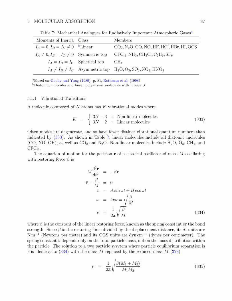
5 MOLECULAR ABSORPTION 87
Table 7: Mechanical Analogues for Radiatively Important Atmospheric Gasesa
Moments of Inertia Class Members
IA = 0, IB = IC 6= 0 bLinear CO2,N2O,CO,NO,HF,HCl,HBr,HI,OCS
IA 6= 0, IB = IC 6= 0 Symmetric top CFCl3,NH3,CH3Cl,C2H6, SF6
IA = IB = IC Spherical top CH4
IA 6= IB 6= IC Asymmetric top H2O,O3, SO2,NO2,HNO3
aBased on Goody and Yung (1989), p. 81, Rothman et al. (1998)bDiatomic molecules and linear polyatomic molecules with integer J
5.1.1 Vibrational Transitions
A molecule composed of N atoms has K vibrational modes where
K =
3N − 3 : Non-linear molecules3N − 2 : Linear molecules (333)
Often modes are degenerate, and so have fewer distinct vibrational quantum numbers thanindicated by (333). As shown in Table 7, linear molecules include all diatomic molecules(CO, NO, OH), as well as CO2 and N2O. Non-linear molecules include H2O, O3, CH4, andCFCl3.
The equation of motion for the position r of a classical oscillator of mass M oscillatingwith restoring force β is
Md2r
dt2= −βr
r+β
M= 0
r = A sinωt+B cosωt
ω = 2πν =
√β
M
ν =1
2π
√β
M(334)
where β is the constant of the linear restoring force, known as the spring constant or the bondstrength. Since β is the restoring force divided by the displacement distance, its SI units areN m−1 (Newtons per meter) and its CGS units are dyn cm−1 (dynes per centimeter). Thespring constant β depends only on the total particle mass, not on the mass distribution withinthe particle. The solution to a two particle sysytem where particle equilibrium separation isr is identical to (334) with the mass M replaced by the reduced mass M (323)
ν =1
2π
√β(M1 +M2)
M1M2
(335)

5 MOLECULAR ABSORPTION 88
The bond strength β depends on the exact arrangement of nuclei within a molecule. Fordiatomic molecules β approximately fits the following progression: Single bond, double bond,and triple bond diatomic molecules have β of approximately 500, 1000, and 1500N m−1(5×10⁵, 10× 105, and 15× 105 dyn cm−1) respectively.
Let us consider the aborption spectrum due to stretching of the carbon monoxide molecule.CO is approximately a triply bonded diatomic molecule with a bond strength of about1900 N m−1. We will use (335) to predict the fundamental frequency νCO of the absorptionspectrum. We shall include the details of the calculation to demonstrate the equivalence ofthe results obtained using SI and CGS units.
νCO ≈ 1
2π
√1900N m−1 × (12.0× 10−3 + 16.0× 10⁻³) kg mol−1
12.0× 10⁻³ kg mol−1 × 16.0× 10−3 kg mol−1
≈ 1
6.28
√53.2N m−1
192× 10−6 kg mol−1 ≈ 0.160
√2.77× 10⁵
kg ms2× 1
m× N
kg
νCO ≈ 84.2
√1
s2× 6.02× 1023
1≈ 65.3× 10¹² s−1 = 65.3THz
λCO =c
νCO
≈ 3.00× 10⁸ m s−1
65.3× 10¹² s−1 = 4.59× 10⁻⁶ m = 4.59µm
νCO =νCO
100c≈ 65.3× 10¹² s−1
100 cm m−1 × 3.00× 108 m s−1 ≈ 2182 cm−1 (336)
The conversion of νCO to νCO and λCO is straightforward, and shows that the stretchingmode of the CO molecule produces an absorption spectrum in the infrared. For pedagogicalreasons, let us repeat the derivation of νCO using CGS units to demonstrate that neithersystem is clearly superior in terms of its simplicity or ease of manipulation.
νCO ≈ 1
2π
√1.9× 10⁶ dyn cm−1 × (12.0 + 16.0) g mol−1
12.0 g mol−1 × 16.0 g mol−1
≈ 1
6.28
√53.2× 10⁶ dyn cm−1
192 g mol−1 ≈ 0.160
√27.7× 10⁴
g cms2× 1
cm× N
g
and the rest of the computation is identical to (336). It appears that CGS units, historicallythe system of choice for radiative transfer, are slightly more simple to work with than SI unitsbecause of the CGS-centric definition of atomic weights. However, in this era of automatedcomputations, the slight advantage of CGS does not appear to outweigh the usefulness ofconsistently using SI units (336). All other things being equal, we recommend using SI unitswherever practical in radiative transfer, a convention we follow in this text.
The vibrational energy of a quantum harmonic oscillator is
Ev =K∑k=1
hνk(vk +12) (337)
where νk is the frequency of the kth mode, hνk is the vibrational constant of the mode,and vk is the vibrational quantum number of the mode. Like other quantum numbers, v
5 MOLECULAR ABSORPTION 89
is an integer v ∈ [0, 1, 2, . . .]. The term of 12
in (337) is called the zero-point energy. Thevibrational ground state of a molecule is reached when vk = 0 for all K vibrational modes.The linear relation between vk and Ev (337) is an approximation. In reality anharmonicitiescause oscillations to deviate from linear behavior. This causes vibrational energy levels tobecome more closely spaced as vk increases.
Allowed transitions must match applicable selection rules. The selection rule for vibra-tional transitions is
∆v = v′ ± v′′ = ±1 (338)
The fundamental transition refers to transitions between the first excited state (v = 1) andthe vibrational ground state (v = 0). Using ∆v = ±1 in (337) leads to
∆Ev = hνk(v + 1 + 12)− hνk(v +
12)
= h[νk(v +32)− νk(v + 1
2)]
= hνk (339)
For simpler molecules such as diatomic molecules, the relation between the type of vibrationalmode k (e.g., stretching, bending) and the fundamental energy of the mode (339) may dependon only a few parameters.
5.1.2 Isotopic Lines
The quantum mechanical analogue of (334) is
νk =1
2π
√β
M(340)
where now β is the force constant of vibrational mode k which depends on the distributionof charge in the molecule but is completely independent of the mass distribution, and thusindependent of isotope. Two distinct isotopes i and j of the same species will thus havediffering equilibrium frequencies νi and νj for the same vibrational mode:
νiνj
=
√Mj
Mi
(341)
For instance, the frequency shift for 13C16O relative to the 2140 cm−1 band of 12C16O is47.7 cm−1.
5.1.3 Combination Bands
Transition selection rules for many important molecules (including all diatomic molecules),require that ∆v 6= 0 and ∆J 6= 0, i.e., vibrational transitions must occur simultaneouslywith rotational transitions. Thus simultaneous transitions of both vibrational and rotationalstates are the norm, not the exception, in the atmosphere. These simultaneous transitions

5 MOLECULAR ABSORPTION 90
form what are called combination bands or vibration-rotation bands. The energy of suchtransitions is obtained by subtracting the lower energy state from the upper energy state
νR = νk +B′vJ
′(J ′ + 1)−B′′vJ
′′(J ′′ + 1)J2 (342)
where νk is the energy of the pure vibrational transition (337). We have not cancelled liketerms, as in the idealized case of (331), since B′
v 6= B′′v in combination bands. Substituting
∆J = ±1 into (342) leads to the energy spacings between the R-branch transitions and theP-branch transitions, respectively.
νR = νk + 2B′v + (3B′
v −B′′v)J + (B′
v −B′′v)J
2 (343)νP = νk − (B′
v +B′′v)J + (B′
v −B′′v)J
2 (344)
There may be a number of absorption bands in addition to the fundamental bands of amolecule. These include overtone bands, combination bands, vibration-rotation bands, andharmonic coupling bands. Overtone bands occur at frequencies which are multiples of thefundamental frequencies. Combination bands are due to the interaction of two fundamentalvibration bands. The combined frequency …Vibration-rotation bands have already beendiscussed. Harmonic coupling bands occur when interactions among closely spaced oscillationfrequencies produces distinct, unexpected bands. This is relatively uncommon.
5.2 Partition FunctionsThe statistical weight g measures the number of available states in a given quantum con-figuration. Quantum theory teaches us that rotational energy levels are 2J + 1 degenerateowing to 2J + 1 indistinguishable orientations of the component of angular momentum in afixed direction in space. The statistical weight for rotational levels is therefore
gr = 2J + 1 (345)
In LTE, rotational states are populated according to Boltzmann statistics, so that theprobability of occupancy is proportional to e−Er/kT . At temperature T , the ratio of moleculesin state J ′ to those in state J ′′ is therefore
N(J ′)
N(J ′′)≡ gJ ′
gJ ′′
e−Er(J ′)/kT
e−Er(J ′′)/kT
=2J ′ + 1
2J ′′ + 1exp
−hcBv
kT[J ′(J ′ + 1)− J ′′(J ′′ + 1)]
(346)
where now J ′ and J ′′ refer to any values of J , not just those satisfying selection rules.To examine the fractional abundance of molecules in state J relative to those in all otherrotational states, we must sum (346) over all J ′′ while holding J ′ = J fixed. This leads to
N(J)
N=
2J + 1
Qr
exp
[−hcBv
kTJ(J + 1)
](347)

5 MOLECULAR ABSORPTION 91
where we have defined the rotational partition function Qr as the total, probability-weightednumber of available rotation states in the system
Qr =∞∑J=1
(2J + 1) exp
[−hcBv
kTJ(J + 1)
](348)
For atmospheric cases of interest, kT hcBv so the exponential term becomes vanishinglysmall. To express and evaluate (348) as an integral, we make a change of variables
x =hcBv
kTJ(J + 1)
dx =hcBv
kT(2J + 1)dJ
(2J + 1)dJ =kT
hcBv
dx (349)
This maps J ∈ [0,∞) to x ∈ [0,∞). Thus x is considered a continuous function of J .Substituting (349) into (348) results in
Qr ≈∫ ∞
0
(2J + 1) exp
[−hcBv
kTJ(J + 1)
]dJ
=
∫ ∞
0
kT
hcBv
e−x dx
=kT
hcBv
[−e−x
]∞0
=kT
hcBv
[−0− (−1)]
=kT
hcBv
(350)
Substituting (350) into (347) we obtainN(J)
N=
hcBv(2J + 1)
kTexp
[−hcBv
kTJ(J + 1)
](351)
Examination of (351) shows that N(J)/N is small for J → 0 and for J →∞ and maximalin between. The derivation of (351) neglected any vibrational-dependence of Bv.
The vibrational partition function Qv is defined by a procedure analogous to (346)–(350).Contrary to rotational states (345), vibrational states all have equal statistical weights
gv = g0 (352)
In LTE, Boltzmann’s Law, (352) and (337) lead to
N(v′)
N(v′′)≡ gv′
gv′′
e−Ev(v′)/kT
e−Ev(v′′)/kT
=g0g0
exp
−[hν0(v
′ + 12)
kT−
hν0(v′′ + 1
2)
kT
]= exp
[−hν0kT
(v′ − v′′)]
(353)
5 MOLECULAR ABSORPTION 92
Notice that the statistical weight and the zero-point energy contribution of hν0/2 factor outof the relative abundance of molecules in a given vibrational level (353). Nevertheless, thezero-point energy does contribute to the total internal energy of the system and so is properlyincluded in the definition of the vibrational partition function Qv
Qv =∞∑v=0
exp
[−hν0kT
(v + 12)
]= e−hν0/2kT
∞∑v=0
(e−hν0/kT
)v=
e−hν0/2kT
1− e−hν0/kT(354)
where in the last step we used the solution for an infinite geometric series whose ratio betweenterms r < 1,
∞∑n=0
a0rn =
a01− r
(355)
The fractional abundance of molecules in vibrational state v is thus
N(v)
N=
1
Qv
exp
[−hν0kT
(v + 12)
]=
1− e−hν0/kT
e−hν0/2kTe−hν0/2kT e−vhν0/kT
= (1− e−hν0/kT )e−vhν0/kT (356)
Vibrational levels are so widely spaced that most molecules in the lower atmosphere are inv = 0 or v = 1 states.
It is common to approximate the total internal partition function of atmospheric transi-tions Q as the product of the vibrational and the rotational partition functions. Using (354)and (350) we obtain
Q ≈ QvQr
≈ e−hν0/2kT
1− e−hν0/kT
kT
hcBv
In the high temperature limit where kT hν0 then we may use the behavior e−x ≈ 1 − xso this becomes
Q ≈1− hν0
2kT
1− 1 + hν0kT
kT
hcBv
≈2kT−hν0
2kThν0kT
kT
hcBv
≈ 2kT − hν02hν0
kT
hcBv
5 MOLECULAR ABSORPTION 93
5.3 Dipole RadiationThe probability Pif of absorption of a photon leading to a change in molecular state fromstate i to state f is
Pif = t
(e2
hc3m2e
) 2∑α=1
∮ [ωNα(k)|〈ψf |eik·reα(k) · p|ψi〉|2
]fi
dΩ (357)
The matrix element 〈ψf |eik·reα(k) · p|ψi〉 determines the absorption probability. The dipoleapproximation retains only the first term in the expansion
eik·r = 1 + ik · r + · · ·
so that the matrix element simplifies to
〈ψf |eik·reα(k) · p|ψi〉 = eα · 〈ψf |p|ψi〉 (358)
This matrix element is related to the line strength S as follows (Rothman et al., 1998,p. 709)....
5.4 Two Level AtomEinstein created an elegant paradigm for analyzing the interaction of matter and radiation.His tool is called the two level atom. It consists of an ensemble of molecules with twodiscrete energy levels, E1 and E2 > E1. The energy levels have statistical weights g1 andg2, respectively. There are n1 molecules per unit volume in the state with E1, and n2 in thestate with E2. The frequency of transition between the two levels is hν0 = E2 − E1.
The five processes by which an idealized two-level molecule may change state are
n2A21−→ n1 + hν0 (359)
n1 + hν0B12−→ n2 (360)
n2 + hν0B21−→ n1 + 2hν0 (361)
n2 +M+KEC21−→ n1 +M+KE′ + hν0 (362)
n1 +M+KEC12−→ n2 +M+KE′ (363)
where M is a collision partner and KE and KE′ represent the kinetic energy of the twomolecule system before and after the collision, respectively. The most frequent collisionpartners are, naturally, nitrogen and oxygen molecules.
The Einstein coefficient A21 s−1 is the transition probability per unit time for spontaneousemission. Spontaneous emission, as its name implies, requires no external stimulus. Thusdecay of excited molecules occurs even in the absence of a radiation field. Each emissionreduces the population of excited molecules and increases the population of ground statemolecules by one. Hence
dn1
dt= A21n2 (364)
5 MOLECULAR ABSORPTION 94
The Einstein coefficient B12 determines the rate of radiative absorption. B12 is also calledthe Einstein coefficient for stimulated absorption. More specifically, B12 is the proportionalityconstant between the mean intensity of the radiation field Iν and the probability per unit timeof an absorption occuring. The transition probability per unit time for radiative absorptionis B12Iν . B12 has units of [s−1(W m−2 sr−1 Hz−1)−1]. The rate of radiative absorptions perunit time per unit volume is
dn2
dt= n1
∫ ∞
0
∫Ω
α(ν)Iνhν
dΩdν
= 4πn1
∫ ∞
0
α(ν)Iνhν
dν (365)
where α(ν) refers to absorption cross-section of the single transition available in the two-levelatom. Comparing the final two expressions we see that
B12 =4πα(ν)
hνΦ(ν)(366)
B12 is intimately related to the line strength S of the molecular transition (Rothman et al.,1998, p. 709). In particular, B12 may be expressed in terms of the weighted transition-moment squared.
The Einstein coefficient B21 determines the rate of stimulated emission or induced emis-sion. B21Iν is transition probability per unit time for stimulated emission. B21 has the samedimensions as B12.
dn1
dt= n2
∫ ∞
0
∫Ω
αs(ν)Iνhν
dΩdν
= 4πn2
∫ ∞
0
αs(ν)Iνhν
dν (367)
where αs(ν) is the absorption cross-section for stimulated emission.Gaseous absorption cross-sections α(ν) are extremely narrow and so the integrals over
frequency domain in (365) and (367) are determined by a small range of frequencies aboutν0, the line center frequency. Exact descriptions of line broadening about ν0 are discussedin §4.1.2–§4.1.5. It is instructive to ignore the details of the finite shape of line transitionsfor now and to assume the line absorption cross section behaves as a delta-function withintegrated cross section a12
α(ν) ≈ a12δ(ν − ν0) (368)
a12 =πe2
mec(369)
where me is the electron rest mass, e is the electron charge, and f is the oscillator strengthof the transition. With these definitions.
In thermodynamic equilibrium the number of transitions from state 1 to state 2 per unittime per unit volume equals the number of transitions from state 2 to state 1 per unit time

5 MOLECULAR ABSORPTION 95
Table 8: hitran databaseab
This Text hitran DescriptionSi,0 Sηη′ Line strengthαi,0 γair Pressure-broadened HWHM
γself Self-broadened HWHMν0 νηη′ Transition frequencyν ′′i Eν Lower state energyn n Exponent in temperature-dependence of pressure-broadened halfwidthδ δ Air-broadened pressure shift of transition frequency ν0ν ν Frequency in wavenumbers
aEquivalance between symbols employed in this work and those used by Rothman et al. (1998), Ap-pendix A.
bhitran data are tabulated at a temperature T0 and pressure p0 of 296K and 101325.0Pa, respectively.
per unit volume. Combining (364), (365), and (367) we obtain
dn1
dt=
dn2
dtn1B12Iν = n2A21 + n2B21Iν (370)
5.5 Line StrengthsWe repeat the definition of line strength (272) for convenience
S =
∫ ∞
0
α(ν) dν (371)
In practice, (371) is either measured in the laboratory or predicted from ab initio methods.
5.5.1 hitran
The hitran (“high-resolution transmission”) database provides the parameters required tocomputed absorption coefficients for all atmospheric transitions of interest. The hitrandatabase is defined by Rothman et al. (1998), and its usage is defined in their Appendix A.
The idiosyncratic units of line parameters can be confusing. Most hitran data are pro-vided in CGS units. For reference, Table 8 presents the equivalence between the symbolsused in Rothman et al. (1998), their Appendix A, and our symbols.
The line strength Si,0 (272) is tabulated in hitran in CGS units of wavenumbers times cen-timeter squared per molecule, cm−1 cm2 molecule−1, often written cm atm−1. Line strengthsfor weak lines can be less than 10−36 cm−1 cm2 molecule−1, i.e., unrepresentable as IEEEsingle precision (4 byte) floating point numbers. Thus it is more robust to work with Si,0

5 MOLECULAR ABSORPTION 96
units of per mole (rather than per molecule) in applications where using IEEE double pre-cision (8 byte) floating point numbers is not an option either due to memory limitationsor computational overhead. Following are the conversions from the tabulated values of Si,0in cm−1 cm2 molecule−1 to more useful units, including cm−1 m2 molecule−1, cm−1 m2 mol−1,and to fully SI units of Hz m2 mol−1 and m m2 mol−1.
Si,0[cm−1 m2 molecule−1] = Si,0[cm−1 cm2 molecule−1]× 10−4 (372a)Si,0[cm−1 m2 mol−1] = Si,0[cm−1 cm2 molecule−1]× 10−4 ×N (372b)Si,0[Hz m2 mol−1] = Si,0[cm−1 cm2 molecule−1]× 10−4 × 100c×N (372c)Si,0[m m2 mol−1] = Si,0[cm−1 cm2 molecule−1]× 10−4 × 100λ2 ×N (372d)
where N is Avagadro’s number. Equation (372d) is uncertain.The energy of the lower state of each transition, E ′′
i , is required to determine the relativepopulation of that state available for transitions. hitran supplies this energy in wavenumberunits in the tabulated parameter ν ′′i which is simply related to E ′′
i by
E ′′i = hcν ′′i (373)
Of course, consistent with hitran and spectroscopic conventions, ν ′′i is archived in CGS, cm−1.All hitran data have been scaled from the conditions of the experiment to a temperature
and pressure of 296K and 1013.25mb, respectively. Thus line strengths must typically bescaled from hitran-standard conditions, Si,0(T0), to the atmospheric conditions of interest,Si(T ).
Si(T ) = Si,0(T0)Q(T0)
Q(T )
e−hcνi/kT
e−hcνi/kT0
1− e−hcνij/kT
1− e−hcνij/kT0(374)
where Q is the total internal partition function. The second, third and fourth factors onthe RHS of (374) are the temperature-dependent scalings of, respectively, the total partitionfunction, the Boltzmann factor for the lower state, and the stimulated emission factor. Thescaling presented in (374) is general and contains no approximation.
The classical approximation (Rogers and Yau, 1989; Thomas and Stamnes, 1999) assumesthat Q is the product of the rotational and the vibrational partition functions
Q(T ) ≈ Qv(T )Qr(T ) (375)
In this approximation, Qv (354) and Qr (350) are treated as independent components of Q.This allows Q to be computed as discussed in §5.2. Most high precision calculation improvethis approach by using more exact methods described in Gamache et al. (1990) and Gamacheet al. (2000).
For many applications, a simplified version of (374) is employed
Si(T ) = Si,0(T0)
(T0
T
)mexp
[−E
′′i
k
(1
T− 1
T0
)]= Si,0(T0)
(T0
T
)mexp
[E ′′i
k
(1
T0
− 1
T
)](376)
5 MOLECULAR ABSORPTION 97
where m is an empirical parameter of order unity and The parameterization (376) incorpo-rates the temperature dependence of both partition functions and the stimulated emissionfactor into the single factor (T0/T )
m. The exact temperature dependence of Boltzmann fac-tors is retained. If the parameter m is available, use of (376) offers decreased computationaloverhead relative to (374).
Pressure-broadened halfwidths αp,0 are also provided at the reference temperature andpressure, αp,0 ≡ αp(p0,T0). hitran literature refers to broadening features are as air-broadened (rather than pressure-broadened) because all parameters in the hitran databaseare normalized to Earth’s natural isotopic mixing ratios. Thus while the broadening pro-cess is collision-broadening, the tabulated line width refers to collision-broadening by air ofEarth’s isotopic composition, hence the label. hitran actually provides two halfwidths, theself-broadened halfwidth αs,0 and the air-broadened or foreign-broadened halfwidth αf,0. Air-broadening accounts for collision-broadening by foreign molecules, i.e., all molecules exceptthe species undergoing radiative transition. Thus air-broadening is, to a good approximation,due nitrogen and oxygen molecules. The other form of broadening, self-broadening refersto collision-broadening by molecules of the species undergoing the radiative transition. Be-cause reasonances may develop between members of identical species, in general αs,0 6= αf,0.The pressure-broadened halfwidth of transitions of radiatively active species A at arbitrarypressure and temperature scales as
αp(p, T ) =
(T0
T
)n(p− pAp0
αf,0 +pAp0
αs,0
)(377)
where n is an empirical fitting parameter supplied by hitran and pA is the partial pressureof species A. Clearly self-broadening effects are appreciable only for species with signifcantpartial pressures, i.e., O2 and N2. For minor trace gases, pA p and pA p0 so p− pA ≈ pand pA/p0 ≈ 0. For such gases, (377) simplifies to
α(p, T ) ≈ α0p
p0
(T0
T
)n(378)
which has no dependence on self-broadening.Collision-broadening may also cause a pressure-shift of the line transition frequency away
from the tabulated line center frequency ν0 = ν(p0) to a shifted frequency ν∗ = ν(p). hitransupplies a parameter δ(p0) in CGS wavenumbers per atmosphere (cm−1 atm−1) with whichto calculate the line center frequency change due to pressure-shifting.
ν∗(p) = ν0 + δ(p0)p
p0
(379)
The prescriptions for adjusting line centers (379) and half-widths (377) from (p0,T0) toto arbitrary p and T should be used to determine the corrected line shape profile of eachtransition considered. In the lower atmosphere, application of (379) and (377) leads to acorrected Lorentzian profile (280)
ΦL(ν, ν0, p, T ) =1
π
αL(p, T )
ν − [ν0 + pδ(p0)/p0]2 + αL(p, T )2
ΦL(ν, ν0, p, T ) =1
π
αL(p, T )
(ν − ν∗)2 + αL(p, T )2(380)
6 BAND MODELS 98
Of course this section has only discussed application of hitran database parameters to at-mospheres in LTE conditions. Application of hitran to nonlocal thermodynamic equilibriumconditions is discussed in Gamache and Rothman (1992).
It is necessary to compute statistics of Si for use in narrow band models (§6). There isno reason not to apply the full approach of (374) when computing these statistics. Certainwell-documented narrow band models use more approximate forms appropriate for specificapplications. Briegleb (1992) uses
Si(T ) = Si,0(T0)
(T0
T
)3/2e−hcνi/kT
e−hcνi/kT0
1− e−hcνij/kT
1− e−hcνij/kT0(381)
which is a hybrid of (374) and (376) with m = 1.5.
5.6 Line-By-Line Models5.6.1 Literature
The classic paper on the water vapor continuum is Clough et al. (1989). Fu and Liou(1992) compare a correlated-k method to line-by-line model results. Ellingson and Wiscombe(1996) describe the a field experiment to directly compared measured and modeled spectralradiances to both band and line-by-line models. Crisp (1997) uses a line-by-line model todetermine atmospheric solar absorption. Sparks (1997) presents an economical algorithmfor selecting variable wavelength grid resolution such that absorption coefficients may becomputed to a given level of accuracy. Mlawer et al. (1997) compare a correlated-k model(rrtm) to the well-known line-by-line model lblrtm. Moncet and Clough (1997) describea fully scattering line-by-line model. Walden et al. (1997) presents test-case spectra forevaluating line-by-line radiative transfer models in cold and dry atmospheres. Vogelmannet al. (1998) use observations to constrain magnitude of any non-Lorentzian continuumin the near-infrared. Partain et al. (2000) discuss the equivalance theorem. Quine andDrummond (2001) present an algorithm that computes absorption coefficients to a specifiederror tolerance by using a pre-computed lookup table of where interpolation is appropriate.
6 Band ModelsBand models, also called narrow band models, discretize the radiative transfer equation in-tervals for which the line statistics and the Planck function are relatively constant. Theliterature describing these models extends back to Goody (1957). Band models have tradi-tionally been applied to thermal source functions (187a)–(187b), but they may also be appliedto the solar spectral region (Zender et al., 1997) (MODTRAN3) if additional assumptionsare made.
6.1 GenericThe following presentation assumes that the absorption path is homogeneous, i.e., at constanttemperature and pressure. Important corrections to these assumptions are necessary ininhomogeneous atmospheres. These corrections are discussed in §6.3.2.

6 BAND MODELS 99
This discussion makes use of an arbitrary frequency interval ∆ν which represents thediscretization interval of narrow band approximation. It is important to remember that ∆νis best determined empirically by comparison of the narrow band approximation to line-by-line approximations. Typically, ∆ν is 5–10 cm−1. Kiehl and Ramanathan (1983) showed∆ν = 5 cm−1 bands are optimal for CO2. Briegleb (1992) uses ∆ν = 5 cm−1 for CO2, O3,CH4, N2O, but ∆ν = 10 cm−1 for H2O. Kiehl (1997) recommends ∆ν = 5 cm−1 for CO2,10 cm−1 for H2O, 5–10 cm−1 for O3, and 5 cm−1 for all other trace gases.
6.1.1 Beam Transmittance
The gaseous absorption optical depth τa(ν) is the product of the spectrally resolved molecularcross-section α(ν) (535a) and the absorber path U (269)
τa(ν) = α(ν)U (382)
The transmittance T (ν) between two points in a homogeneous atmosphere is the negativeexponential of τa(ν) (182),
T (ν) = e−τa(ν)
= e−α(ν)U (383)
Note that T (ν) is the spectrally and directionally resolved transmittance because (a) it per-tains to a monochromatic frequency interval and (b) it applies to radiances, not to irradiances(which require an additional angular integration). Narrow band models are based on themean transmittance T∆ν of a narrow but finite frequency interval ∆ν between ν0 − ∆ν/2and ν0 +∆ν/2.
T∆ν =1
∆ν
∫∆ν
T dν
=1
∆ν
∫∆ν
e−τa dν (384)
where ν0 is the central frequency of the interval in questionUsing (271), we rewrite (384) as
T∆ν =1
∆ν
∫∆ν
exp[−α(ν)U ] dν
If the lines are Lorentzian (i.e., pressure-broadened) then the transmittance may be writtenin terms of the line strength and absorber amount using (273a) and (305)
α(ν)U =SαLU
π(ν2 + α2L)
(385)
Thus (384) becomes
T∆ν =1
∆ν
∫∆ν
exp
[− SαLU
π(ν2 + α2L)
]dν (386)

6 BAND MODELS 100
6.1.2 Beam Absorptance
In analogy to T (181) we define the monochromatic beam absorptance A
A = 1− T= 1− exp[−α(ν)U ] (387)
where α(ν) is the absorption cross-section and U is the absorber path. As described in §6.1.1,we refer to A as the beam absorptance becuase it pertains to a monochromatic frequency,and refers to absorption of radiance, not irradiance.
The band absorptance A∆ν is the complement of the band transmittance
A∆ν = 1− T∆ν=
1
∆ν
∫∆ν
A dν
=1
∆ν
∫∆ν
1− e−τa dν
=1
∆ν
∫∆ν
1− exp[−α(ν)U ] dν (388)
The relation between the band absorptance and band transmittance is the same as the rela-tion between the monochromatic beam absorptance and the monochromatic beam transmit-tance (387). A∆ν measures the mean absorptance within a finite frequency (or wavelength)range comprising many lines. A∆ν does not include any contribution from outside the ∆νrange. Thus A∆ν may neglect contribution from the far wings of some lines in the band.Moreover, it is important to remember that energy absorption follows the band absorptanceonly if the energy distribution within the band is close to linear.
If the line shape is Lorentzian (280), then (386) applies so that
A∆ν =1
∆ν
∫∆ν
1− exp
[− SαLU
π(ν2 + α2L)
]dν (389)
6.1.3 Equivalent Width
The spectrally integrated monochromatic beam absorptance of a line is called its equivalentwidth
W =
∫ +∞
−∞A dν
W (U) =
∫ +∞
−∞1− exp[−α(ν)U ] dν (390)
Thus the absorber amount must be specified in order to determine the equivalent width.The lower limit of integration, −∞, is actually an approximation which is mathematicallyconvenient to retain so that (390) is analytically integrable for the important line shapefunctions. Recall that we are working with a frequency coordinate ν which is defined to beν = 0 at line center ν0 (306). In practice the error caused by using the analytic expressions

6 BAND MODELS 101
resulting from∫ +∞−∞ rather than those resulting from
∫ +∞−ν0 is negligible except for lines in the
microwave.The name “equivalent width” reminds us that W is the width of a completely saturated
rectangular line profile that has the same total absorptance. The relation between U andW (U) is called the curve of growth. The curve of growth of a gas can be measured inthe laboratory. The interpretation of the curve of growth played a very important role inadvancing our understanding and representation of gaseous absorption.
If the line shape is Lorentzian (280), then (389) applies
W =
∫ +∞
−∞1− exp
[− SαLU
π(ν2 + α2L)
]dν (391)
6.1.4 Mean Absorptance
Although the spectrally resolved absorptance (387) and the band absorptance (388) aredimensionless, the equivalent width (390) has units of frequency (or wavelength). It isconvenient to define a dimensionless mean absorptance for a transition line A
A =1
δ
∫ +∞
−∞A dν
=1
δ
∫ +∞
−∞1− exp[−α(ν)U ] dν
=W
δ(392)
where δ is the mean line spacing between adjacent lines in a given band. Note that A∆ν
(388) differs from A (392). A accounts for the absorptance due to a single line over theentire spectrum and renormalizes that to a mean absorptance within a specified frequency(or wavelength) range (δ). In contrast to A∆ν , A does not neglect any absorption in thefar wings of a line. Therefore the sum of the average absorptances of all the lines centeredwithin ∆ν may exceed, by a small amount, the band absorptance computed from (388)
i=N∑i=1
Ai ≥ A∆ν (393)
This difference should make it clear that A is much more closely related to W than to A∆ν .For lines with Lorentzian profiles (280), W and A are
W = Aδ =
∫ +∞
−∞1− exp
[− SαLU
π(ν2 + α2L)
]dν (394)

6 BAND MODELS 102
We shall rewrite (394) in terms of three dimensionless variables, x, y, and u
x = ν/δ (395a)ν = δx
dx = δ−1 dν
dν = δ dx
y = αL/δ (395b)αL = δy
u =SU
2παL
(395c)
SU
π= 2αLu
This change of variables maps ν ∈ [−∞,+∞] to x ∈ [−∞,+∞]. We obtain
A =1
δ
∫ +∞
−∞1− exp
[−(2αLu)
(αL
δ2x2 + δ2y2
)](δ dx)
=
∫ +∞
−∞1− exp
[− 2α2
Lu
δ2(x2 + y2)
]dx
=
∫ +∞
−∞1− exp
[− 2δ2y2u
δ2(x2 + y2)
]dx
=
∫ +∞
−∞1− exp
[− 2uy2
x2 + y2
]dx (396)
The solution to this definite integral may be written in terms of modified Bessel functionsof the first kind Iν(u) (see §10.4)
A = 2πyue−u[I0(u) + I1(u)]
≡ 2πyL(u)
= 2παLδ−1L(u)
W = 2παLL(u) (397)
where L(u) is the Ladenburg and Reiche function (Ladenburg and Reiche, 1913). Thedimensionless optical path u (395) is therefore a key parameter in determining the gaseousabsorptance. Two important limiting cases of (397) are u 1 and u 1.
For small optical paths, SU 1 (269), or, equivalently, u 1 (395c). This is theweak-line limit. In this limit the exponential in (394) or (396) may be replaced by the firsttwo terms in its Taylor series expansion. Thus all line shapes have the same weak-line limit
W = Aδ ≈∫ +∞
−∞α(ν)U dν
≈ SU
∫ +∞
−∞ΦL(ν) dν
≈ SU (398)
6 BAND MODELS 103
where we have use the generic normalization property of the line shape profile (283) in thefinal step.
For large optical paths, SU 1 (269), or, equivalently, u 1 (395c). This is the strongline limit. To examine this limit we first note that the line HWHM is much smaller thanthe frequencies where line absorptance is strong, i.e., αL ν in (394). Equivalently, y x(395a)–(395b) so that y2 may be neglected relative to x2 in the denominator of (396)
A ≈∫ +∞
−∞1− exp(−2uy2/x2) dx
One further simplification is possible. Both terms in the integrand are symmetric about theorigin so we may consider only positive x if we double the value of the integral.
A = 2
∫ +∞
0
1− exp(−2uy2/x2) dx (399)
The change of variables z = 2uy2x−2 maps x ∈ (0,+∞) to z ∈ (+∞, 0)
z = 2uy2x−2 (400a)x = (2u)1/2yz1/2 (400b)
dx = (2u)1/2y(−12)z−3/2 dz
= −2−1/2u1/2yz−3/2 dz (400c)
Substituting this into (399) leads to
A ≈ 2
∫ 0
+∞(1− e−z)(−2−1/2u1/2y)z−3/2 dz
≈ 21/2u1/2y
∫ +∞
0
(1− e−z)z−3/2 dz
≈ y√2u
∫ +∞
0
z−3/2 − z−3/2e−z dz
The first term in the integrand of (401) is directly integrable∫z−3/2 dz = −2z−1/2. The
second term in the integrand of (401) is the complete gamma function Γ(−1/2) =. Section ??describes the properties of gamma functions15.
Combining these results we find that the mean absorptance of an isolated Lorentz linein the strong-line limit (401) reduces to
A ≈ y√2u
(−2z−1/2
∣∣∣∣+∞
0
− (−2√
π)
)= y
√2u(∞+ 2
√π)
= 2y√2πu (401)
15This section is currently in http://dust.ess.uci.edu/facts/aer/aer.pdf.

6 BAND MODELS 104
fxm: The first term must vanish, but how? Substituting (395b)–(395c) into (401)
A ≈ 2(αL
δ
)√2π
√SU
2παL
W = Aδ = 2√SUαL (402)
In the strong line limit we see that the mean absorptance A of an isolated line increasesonly as the square-root of the mass path. Physically, the strong line limit is approached asthe line core becomes saturated and any additional absorption must occur in the line wings.Put another way, transition lines do not obey the exponential extinction law on which oursolutions to the radiative transfer equation are based. One important consequence of thisresult is that complicated gaseous spectra must either be decomposed into a multitude ofmonochromatic intervals, each narrow enough to resolve a small portion of a transition line,or some new statistical means must be developed which correctly represents line absorptionin both the weak line and strong line limits.
In summary, the equivalent width W (390) of an isolated spectral line behaves distinctlydifferently in the two limits (398) and (402)
W = Aδ =
SU : Weak-line limit
2√SUαL : Strong-line limit (403)
6.2 Line DistributionsInspection of realistic gaseous absorption spectra reveals that line strengths in complex bandsoccupy a seemingly continuous distribution space, with line strengths S varying over manyorders of magnitude in a single band. A key point discussed further in Goody and Yung(1989) is that the variabilities in line spacing and in line widths within a band are negligible(and usually order of magnitude smaller) in comparison to the dynamic range of S. A bandcontaining a suitably large number of lines, therefore, may be amenable to the approximationthat the line strength distribution may be represented by a continuous function of S. Theline strength distribution function p(S) is the probability that a line in a given spectralregion will have a line strength between S and S +dS. The function p(S) must be correctlynormalized so that probability of a line having a finite, positive strength is unity∫ ∞
0
p(S) dS = 1 (404)
A number of functional forms for p(S) have been proposed.
6.2.1 Line Strength Distributions
Goody (1952) proposed the exponential line strength distribution, now also known as theGoody distribution
p(S) = S−1 e−S/S (405)
where S is a constant which, in the next section, we show to be equal to the mean lineintensity. A prime advantage of (405) is its arithmetic tractability. The zeroth and first

6 BAND MODELS 105
moments of (405) are both solvable analytically. The following sections use this propertyto demonstrate the absorptive characteristics of line distributions. However, more complexdistributions can improve upon the exponential distribution (405) by better representing theobserved line shape distribution of many important species in Earth’s atmosphere, such asH2O.
Malkmus (1967) proposed an improved, albeit more complex, analytic form for the linestrength distribution function. First we present a simplified, approximate version of this PDFwhich illustrates the essential differences between the Malkmus distribution and simpler linestrength distributions.
p(S) = S−1 e−S/S (406)
The difference with (405) is the prefactor has changed from S−1 to S−1. The S−1 dependenceincreases the number of weaker lines relative to stronger lines, which is an improvement over(405) and simpler distributions (such as the Elsasser or Godson distributions). The Malkmusdistribution (406) is now perhaps the most commonly used line distribution function.
The astute reader will note that (406) is not normalizable on the interval [0,+∞) (cf.§6.2.2). A key point of the Malkmus distribution, therefore, is the truncation or tapering ofp(S) so that statistics of the resulting p(S) are well-behaved. A straightforward line strengthdistribution function with most of the desired properties is the “truncated” distributionwhich is non-zero only between a fixed maximum and minimum line strength, SM and Smin,respectively. By convention, Smin is deprecated in favor of the ratio RS between the maximumand minimum line strengths considered in the band
Smin = SM/RS
RS ≡ SM/Smin (407)
The line strength ratio RS measures the dynamic range of line strengths considered in aband, which can be quite large, e.g., greater than 106 for H2O bands. With this convention,
p(S) =
0 : S < SM/RS
(S lnRS)−1 : SM/RS < S < SM0 : S > SM
(408)
Godson (1953) appears to have been the first to examine (408), although it is closely relatedto the full Malkmus distribution. The normalization of (408) is demonstrated in §6.2.2.Clearly (408) contains no contributions from lines weaker than SM/RS or stronger than SM .The main disadvantage to (408) is that it is discontinuous, and thus more difficult to treatcomputationally.
Malkmus (1967) had the insight to identify the following continuous function
p(S) =e−S/SM − e−RSS/SM
S lnRS
(409)
We shall call (409) the full Malkmus line strength distribution. In practice, (409) is onlyapplied in the limit RS →∞. Rather than simply truncating (406) so that p(S) is non-zeroonly between some lower and upper bound (408), Malkmus (1967) developed (409) becauseit has many useful properties:

6 BAND MODELS 106
1. p(S) is continuous2. p(S) has S−1 dependence over the bandwidth of interest3. p(S) approaches (408)4. p(S) is analytically integrable
Following Malkmus (1967), let us ellucidate the behavior of (409) in important limits. ForlargeRS and SM/RS S SM the bracketed term in (409) approaches unity so that p(S) ≈(S lnRS)
−1, i.e., the behavior is identical to (408). For S SM , p(S) ≈ (S lnRS)−1e−S/SM .
Thus for S SM , p(S) is non-zero but much less than what extrapolating (S lnRS)−1 into
this region would yield. Finally, for large SM and S SM/RS, p(S) ≈ (RS)−1(RS − 1)/SM .
To summarize, the limits of (409) are as follows
p(S) =
(lnRS)
−1(RS − 1)/SM : S SM/RS
(S lnRS)−1 : SM/RS S SM
(S lnRS)−1e−S/SM : S SM
(410)
Thus (409) behaves like (408) everywhere except near the truncation points SM/RS and SM .Beyond these points, (409) is sharply tapered so that lines in these regions do not influencethe statistics of the line strength distribution very much.
6.2.2 Normalization
The normalization properties of the line strength distribution functions will now be shown.The exponential distribution (405) is easily shown to be normalized∫ ∞
0
S−1 e−S/S dS = S−1[−Se−S/S
]∞0
= −0− (−1) = 1 (411)
For heuristic purposes we first demonstrate that the approximate Malkmus distribution(406) is not normalizeable despite its apparent simplicity. With the substitution x = S/Swe have ∫ ∞
0
S−1 e−S/S dS =
∫ ∞
0
x−1 e−x dx (412)
The RHS resembles the complete gamma function of zero, Γ(0) (??). However, Γ(0) isindeterminate, a singularity between negative and positive infinities much like tan π
2. Thus
(406) is not normalizeable.Next we consider the truncated Malkmus distribution (410). We integrate over the non-
zero region, SM/RS to SM , to demonstrate its normalization properties∫ SM
SM/RS
(S lnRS)−1 dS = (lnRS)
−1[lnS]SM
SM/RS
= (lnRS)−1[lnSM − ln(SM/RS)]
= (lnRS)−1[lnSM − lnSM + lnRS]
= 1 (413)
6 BAND MODELS 107
It is more challenging to prove that the full Malkmus distribution (409) is normalized. Tobegin, we simplify p(S) (409) with the substituions a = S−1
M , b = RSS−1M , and thus RS = b/a.∫ ∞
0
p(S) dS = (lnRS)−1
∫ ∞
0
S−1(e−aS − e−bS) dS (414)
We must show, therefore, that this rather complex definite integral always equals ln(b/a) =lnRS. Since both terms in the integrand are of the same form, we shall explicitly evaluateS−1e−aS before subtracting the analogous term involving b. These terms are amenable tointegration by parts with the change of variables
u = e−aS
du = −aeaS dSdv = S−1 dS
v = lnS (415)
The result is
lnRS
∫ ∞
0
S−1e−aS dS =[e−aS lnS
]∞0−∫ ∞
0
lnS(−ae−aS) dS
=[e−aS lnS
]∞0+ a
∫ ∞
0
e−aS lnS dS
The first term on the RHS contains a singularity since ln(0) is undefined. This term however,will disappear once the similar term arising from the integration of
∫S−1e−bS dS is subtracted
from (416). Now we change variables to isolate the parameter a from the dummy variableof integration. Letting x = aS, S = x/a, dx = a dS, and dS = a−1 dx leads to
lnRS
∫ ∞
0
S−1e−aS dS =[e−aS lnS
]∞0+ a
∫ ∞
0
e−x ln(x/a)a−1 dx
=[e−aS lnS
]∞0+
∫ ∞
0
e−x lnx− e−x ln a dx
=[e−aS lnS
]∞0+
∫ ∞
0
e−x lnx dx− ln a[−e−x
]∞0
=[e−aS lnS
]∞0+
∫ ∞
0
e−x lnx dx− ln a[−0− (−1)]
=[e−aS lnS
]∞0+
∫ ∞
0
e−x lnx dx− ln a (416)
There is no closed form solution to the second term on the RHS,∫e−x lnx dx, which is very
close in appearance to the original integral (414). However, this term will also disappear oncethe integration involving b is subtracted from (416). Multiplying both sides by (lnRS)
−1,
6 BAND MODELS 108
and subtracting the integration involving b leads to∫ ∞
0
p(S) dS =1
lnRS
[e−aS lnS
]∞0−[e−bS lnS
]∞0
+
∫ ∞
0
e−x lnx dx−∫ ∞
0
e−x lnx dx− ln a+ ln b
=
ln b− ln a
lnRS
=ln(b/a)
lnRS
=lnRS
lnRS
= 1 (417)
All the like terms in the numerator cancelled in the first step with the exception of lnRS.
6.2.3 Mean Line Intensity
The mean line intensity S of a line strength distribution p(S) is defined as
S =
∫ ∞
0
Sp(S) dS (418)
S is an important statistic of a line strength distribution and any realistic line strengthdistribution should adequately predict S when compared to observed line strengths. Thusmany line strength distributions, e.g., the exponential distribution (405) contain S in theirdefinition. The claim that S is, in fact, the mean strength of these distributions will now beproved.
The mean line intensity of the exponential distribution (405) is∫ ∞
0
Sp(S) dS =
∫ ∞
0
S
Se−S/S dS
=1
S
∫ ∞
0
Se−S/S dS
=1
S
∫ ∞
0
Sxe−xS dx
= S
∫ ∞
0
xe−x dx
= S[−xe−x − e−x
]∞0
= S [−0− 0− (0− 1)]
= S (419)
This demonstrates S is the mean line strength of the exponential distribution.

6 BAND MODELS 109
The mean line intensity of the approximate Malkmus distribution, (406) is∫ ∞
0
Sp(S) dS =
∫ ∞
0
S
Se−S/S dS
=
∫ ∞
0
e−S/S dS
= −Se−S/S∣∣∣∞0
= −S(e−∞/S − e−0/S)
= S (420)
This proves that S is also the mean line strength in the approximate Malkmus line distribu-tion function (406).
The mean line intensity of the full Malkmus distribution is derived directly from (409)∫ ∞
0
Sp(S) dS =
∫ ∞
0
S × e−S/SM − e−RSS/SM
S lnRS
dS
= (lnRS)−1
∫ ∞
0
e−S/SM − e−RSS/SM dS
=1
lnRS
[−SMe−S/SM +
SMRS
e−RSS/SM
]∞0
=SMlnRS
[−0 + 0− (−1)− (R−1
S )]
=SMlnRS
(1−R−1S ) =
SMlnRS
RS − 1
RS
=RS − 1
RS lnRS
SM (421)
This expression for S does not converge in the limit as RS → ∞. Thus the mean linestrength of the Malkmus distribution (409) depends on the parameter RS (??), the ratiobetween the strongest and weakest lines in a given band. It is clear from (421) that Sdecreases as RS increases. Adequately representing the importance of weak lines is one ofthe chief advantages of the Malkmus distribution relative to other distributions.
The maximum line strength intensity SM may be expressed in terms of the mean linestrength S by inverting (421)
SM =RS lnRS
RS − 1S (422)
6.2.4 Mean Absorptance of Line Distribution
This section develops the concept of mean absorptance of a band of non-overlapping lines,whereas §6.1.4 derived the mean absorptance A of an isolated Lorentz line. Since the linesare assumed to be non-overlapping, we may weight the contribution of each line to the mean
6 BAND MODELS 110
absorptance (392) by the normalized line strength probability (404)
W = Aδ =
∫ ∞
0
p(S)
(∫ +∞
−∞A dν
)dS
=
∫ ∞
0
p(S)
∫ +∞
−∞1− exp[−SΦU ] dν dS (423)
Inserting the exponential line strength distribution function (405) for p(S) in (423) andinterchanging orders of integration yields
W = Aδ =
∫ ∞
0
S−1 e−S/S∫ +∞
−∞1− exp[−SΦU ] dν dS
= S−1
∫ +∞
−∞
∫ ∞
0
e−S/S − exp
(−SS− SΦU
)dS dν
= S−1
∫ +∞
−∞
∫ ∞
0
e−S/S − exp(−S(S−1 + UΦ)
)dS dν
= S−1
∫ +∞
−∞
[−Se−S/S + (S−1 + UΦ)−1 exp
(−S(S−1 + UΦ)
)]∞0
dν
= S−1
∫ +∞
−∞
[0 + 0−
(−S × 1 + (S−1 + UΦ)−1 × 1
)]dν
= S−1
∫ +∞
−∞S − (S−1 + UΦ)−1 dν
= S−1
∫ +∞
−∞S − S
1 + SUΦdν
=
∫ +∞
−∞1− 1
1 + SUΦdν
=
∫ +∞
−∞
1 + SUΦ− 1
1 + SUΦdν
=
∫ +∞
−∞
SUΦ
1 + SUΦdν (424)
Thus the mean absorptance of the exponential line distribution depends straightforwardlyon the line shape function. Substituting the Lorentz line shape ΦL(ν) = αL/[π(ν
2 + α2L)]
(280) into (424) we obtain
W = Aδ =
∫ +∞
−∞
αL
π(ν2 + α2L)× SU
1 + SU αL
π(ν2+α2L)
dν
=SUαL
π
∫ +∞
−∞
1
ν2 + α2L
× 1π(ν2+α2
L)+SUαL
π(ν2+α2L)
dν
=SUαL
π
∫ +∞
−∞
1
ν2 + α2L
× π(ν2 + α2L)
π(ν2 + α2L) + SUαL
dν

6 BAND MODELS 111
= SUαL
∫ +∞
−∞
1
π(ν2 + α2L) + SUαL
dν
=SUαL
π
∫ +∞
−∞
1
ν2 + α2L + π−1SUαL
dν
(425)
Letting a =√α2L + π−1SUαL = αL
√1 + SU/(παL) and noting that
∫(x2 + a2)−1 dx =
a−1 tan−1(x/a),
W = Aδ =SUαL
π
∫ +∞
−∞
1
ν2 + a2dν
=SUαL
π
1
a
[tan−1 x
a
]+∞
−∞
=SUαL
π
[αL
(1 +
SU
παL
)1/2]−1 [
π
2−(−π
2
)]= SU
(1 +
SU
παL
)−1/2
W
δ= A =
SU
δ
(1 +
SU
παL
)−1/2
(426)
In addition to U , the mean band absorptance A depends on only two statistics of the band,namely S/δ and S/(παL).
We recall that (426) is based on the idealized, continuous line strength distribution (405)rather than on real (observed) line strengths. Observed line strengths and positions aretabulated in the hitran database (§5.5.1). Therefore we may compute any desired statistics ofthe actual line strength distribution. Of particular interest is the observed mean absorptanceof a band in both the weak and strong line limits. Summing (398) and (402) over the Nlines in the given band
W = Aδ =
N−1
∑Ni=1 SiU : SU 1
N−1∑N
i=1 2√SiUαL,i : SU 1
(427)
The weak and strong line limits of the mean absorptance of the exponential line strengthdistribution function (426) are
limSU1
W = Aδ ≈ SU (428a)
limSU1
W = Aδ ≈ SU
(SU
παL
)−1/2
=√
πSUαL (428b)
We now require (428) to equal (427) in the appropriate limits. In the weak line limit
SU = N−1
N∑i=1
SiU
S
δ= (Nδ)−1
N∑i=1
Si (429)

6 BAND MODELS 112
In the strong line limit
√πSUαL = N−1
N∑i=1
2√SiUαL,i
πSUαL =4U
N2
(N∑i=1
√SiαL,i
)2
1
πSαL
=N2
4
(N∑i=1
√SiαL,i
)−2
1
πSαL
× S2 = S2 × N2
4
(N∑i=1
√SiαL,i
)−2
S
παL
=1
N2
(N∑i=1
Si
)2
× N2
4
(N∑i=1
√SiαL,i
)−2
S
παL
=1
4
(N∑i=1
Si
/ N∑i=1
√SiαL,i
)2
(430)
The tractable analytic form of (426) led to its adoption as the dominant formulationfor band models for many years. The mean band absorptances A of other line strengthdistributions have forms similar to (426).
Inserting the Malkmus line strength distribution function (409) for p(S) in (423) andinterchanging orders of integration yields
W = Aδ =
∫ ∞
0
e−S/SM − e−RSS/SM
S lnRS
∫ +∞
−∞1− exp(−SΦU) dν dS
=1
lnRS
∫ +∞
−∞
∫ ∞
0
1
S(e−S/SM − e−SRS/SM )(1− e−SΦU) dS dν
=1
lnRS
∫ +∞
−∞
∫ ∞
0
e−S/SM
S− e−SRS/SM
S+
e−S(ΦU+RS/SM )
S− e−S(ΦU+1/SM )
SdS dν
The first two terms and the last two terms in the integrand are both of the form S−1(e−aS −e−bS). In proving the Malkmus distribution is correctly normalized (414)–(417) we showedthe value of this type of definite integral is ln(b/a). For the first two terms, a = S−1
M andb = RS/SM . For the final two terms, a = ΦU +RS/SM and b = ΦU + 1/SM . Therefore theintegration over S is complete and results in
W = Aδ =1
lnRS
∫ +∞
−∞lnRS + ln
(ΦU + 1/SMΦU +RS/SM
)dν
=1
lnRS
∫ +∞
−∞lnRS + ln
(1 + SMΦU
RS + SMΦU
)dν
=1
lnRS
∫ +∞
−∞lnRS + ln
[(1
RS
)1 + SMΦU
1 + SMΦU/RS
]dν

6 BAND MODELS 113
=1
lnRS
∫ +∞
−∞lnRS + ln
(1 + SMΦU
1 + SMΦU/RS
)− lnRS dν
=1
lnRS
∫ +∞
−∞ln
(1 + SMΦU
1 + SMΦU/RS
)dν (431)
The mean absorptance of the Malkmus distribution also depends simply on the line shapeΦ(ν). The mean absorptance of the exponential line distribution (424) is analogous tothe Malkmus result (431). Note that the former is a rational function of the mean lineintensity S, while the latter depends logarithmically on S. Moreover, the mean absorptanceof the Malkmus distribution depends on the additional parameter RS, the ratio between themaximum and minimum line strengths with the band. The dependence is problematic inthat (431) is not self-evidently convergent as RS → ∞. We now show that for the mostimportant line shapes, A(431) does converge in this limit.
Substituting the Lorentz line shape ΦL(ν) = αL/[π(ν2 + α2
L)] (280) into (424) we obtain
W = Aδ =1
lnRS
∫ +∞
−∞ln
(1 + SMUαL
π(ν2+α2L)
1 + SMUαL
π(ν2+α2L)RS
)dν
=1
lnRS
∫ +∞
−∞ln
(SMUαL + π(ν2 + α2
L)
SMUαLR−1S + π(ν2 + α2
L)
)dν
=1
lnRS
∫ +∞
−∞ln
(ν2 + α2
L + SMUαL/π
ν2 + α2L + SMUαL/(πRS)
)dν
=1
lnRS
∫ +∞
−∞ln
(ν2 + α2
L +SMUαL
π
)− ln
(ν2 + α2
L +SMUαL
πRS
)dν (432)
We simplify (432) by making the substitutions c2 = α2L + SMUαL/π and d2 = α2
L +SMUαL/(πRS), or, equivalenty
c = αL
√1 +
SMU
παL
(433a)
d = αL
√1 +
SMUαL
παLRS
(433b)
With these definitions, (432) becomes
W = Aδ =1
lnRS
∫ +∞
−∞ln(ν2 + c2)− ln(ν2 + d2) dν (434)
This is the difference of two identical, standard integrals (e.g., Gradshteyn and Ryzhik, 1965,p. 205) and reduces to elementary functions∫
ln(ν2 + a2) dν = ν ln(ν2 + a2)− 2ν + 2ν tan−1 ν
a(435)
It is straightforward to differentiate (435) and verify the result. Using (435) to complete thefrequency integration in (434) results in
W = Aδ = (lnRS)−1[ν ln(ν2 + c2)− 2ν + 2c tan−1 ν
c− ν ln(ν2 + d2) + 2ν − 2d tan−1 ν
d
]+∞
−∞
= (lnRS)−1[2c tan−1 ν
c− 2d tan−1 ν
d
]+∞
−∞

6 BAND MODELS 114
The mutual cancellation of the 2ν terms is obvious, but the equivalence of the logarithmicterms may not be self-evident. Consider, however, that both c and d (433) are finite-valuedas ν → ±∞, and it is clear that these terms must cancel. Evaluating the remaining termsleads to
W = Aδ = (lnRS)−12c
π
2− 2d
π
2−[2c(−π
2
)− 2d
(−π
2
)]= (lnRS)
−1(πc− πd+ πc− πd)
= (lnRS)−12π(c− d)
=2παL
lnRS
(√1 +
SMU
παL
−√
1 +SMU
παLRS
)(436)
Although (436) does convey the behavior of the mean absorptance of the Malkmus bandmodel with Lorentzian lines, the presence of the SM term and the RS term is undesirablebecause their values are interrelated and depend on the specific gaseous absorption bandbeing considered. It would be more convenient to express the mean absorptance in terms ofuniversal statistics applicable to all band models, so that A and W may be easily intercom-pared among band models. The mean line strength S (418) appears in both the exponential(405) and Godson line strength distributions. We use (422) to replace SM by S in (436)
W = Aδ =2παL
lnRS
√1 +SU
παL
RS lnRS
RS − 1−
√1 +
SU
παLRS
RS lnRS
RS − 1
=
2παL
lnRS
√1 +SU
παL
RS lnRS
RS − 1−
√1 +
SU
παL
lnRS
RS − 1
(437)
The weak line limit of the mean absorptance of the Malkmus line strength distributionfunction (437) is obtained by expanding the radical into a Taylor series and retaining onlythe first two terms limx1
√1 + x ≈ 1 + x/2
limSU1
W = Aδ ≈ 2παL
lnRS
(1 +
SU
2παL
RS lnRS
RS − 1− 1− SU
2παL
lnRS
RS − 1
)=
2παL
lnRS
× SU lnRS(RS − 1)
2παL(RS − 1)
= SU (438)
which is identical to (428a). The strong line limit of (437) is
limSU1
W = Aδ ≈ 2παL
lnRS
√ SU
παL
RS lnRS
RS − 1−
√SU
παL
lnRS
RS − 1
=
2παL
lnRS
√SU lnRS
παL
(√RS
RS − 1−√
1
RS − 1
)
6 BAND MODELS 115
= 2
(παLSU
lnRS
)1/2( √RS√
RS − 1− 1√
RS − 1
)= 2
√παLSU ×
√RS − 1√
(RS − 1) lnRS
(439)
Let us encapsulate the RS-dependence into the function χ(RS) and and also present χ2(RS)for future use.
χ(RS) =
√RS − 1√
(RS − 1) lnRS
(440a)
[χ(RS)]2 =
(√RS − 1)(
√RS − 1)
(RS − 1) lnRS
=(√RS − 1)(
√RS − 1)
(√RS − 1)(
√RS + 1) lnRS
χ2(RS) =
√RS − 1
(√RS + 1) lnRS
(440b)
where we have made use of the factoring RS − 1 = (√RS − 1)(
√RS + 1). Rewriting (439)
with χ(RS) (440a)
limSU1
W = Aδ ≈ 2√
παLSUχ(RS) (441)
The strong line limit of the Malkmus distribution of Lorentzian lines (441), and the strongline limit of an individual Lorentzian line (403), differ by the factor
√πχ(RS).
The advantage of encapsulating the RS-dependence in the χ(RS) function is that theweak and strong line limits of the Malkmus distribution may now be cast in exactly thesame notation as the exponential distribution (428). First introduce a transformed meanline intensity ˜S and mean line spacing ˜δ which are defined in terms of the line strength ratioof the Malkmus distribution
˜S =S
πχ2↔ S = π
˜Sχ2 (442a)
˜δ =δ
πχ2↔ δ = π
˜δχ2 (442b)
The definitions (442) ensure that S/δ = ˜S/˜δ. In terms of the original mean line strength andspacing, and the transformed line strength and line spacing, the weak and strong line limitsof the mean absorptance A of the Malkmus line strength distribution applied to Lorentzianlines (437) is
limSU1
W = Aδ ≈ SU
δ=
˜SU˜δ
(443a)
limSU1
W = Aδ ≈ 2√
παLSUχ(RS) = 2
√αL
˜SU (443b)

6 BAND MODELS 116
We now rewrite the mean absorptance (437) in terms of the transformed parameters ˜S
and ˜δ (442), making use of (440b)
W
δ= A =
2παL
δ lnRS
√1 +SU
παL
RS lnRS
RS − 1−
√1 +
SU
παL
lnRS
RS − 1
=
1
π˜δχ2
2παL
lnRS
√1 +πχ2 ˜SU
παL
RS lnRS
RS − 1−
√1 +
πχ2 ˜SU
παL
lnRS
RS − 1
=
(√RS + 1) lnRS√RS − 1
2αL
˜δ lnRS
√1 +˜SU
αL
×√RS − 1
(√RS + 1) lnRS
× RS lnRS
(√RS − 1)(
√RS + 1)
−
√1 +
˜SU
αL
×√RS − 1
(√RS + 1) lnRS
× lnRS
(√RS − 1)(
√RS + 1)
=
2αL
˜δ
(√RS + 1√RS − 1
)√1 +˜SU
αL
× RS
(√RS + 1)2
−
√1 +
˜SU
αL
× 1
(√RS + 1)2
=
2αL
˜δ
(√RS + 1√RS − 1
)√1 +˜SU
αL(1 + 1/√RS)2
−
√1 +
˜SU
αL(1 +√RS)2
The asymmetric nature of the optical path terms under the radicals in (444) is clear. Forlarge RS, the first absorptance term approaches a finite-valued function of ˜S, U , and αL. Thesecond absorptance term, on the other hand, approaches unity. Thus the mean absorptanceA asymptotes to a finite value as RS → ∞. Formally, this amounts to taking the limit as√RS 1
W
δ= A ≈ 2αL
˜δ
(√RS√RS
)√1 +˜SU
αL(1 + 0)−√1 + 0
=
2αL
˜δ
√1 +˜SU
αL
− 1
(444)
To obtain W and A in terms of S and δ we use (440a) in (444)
W
δ= A = 2αL ×
πχ2
δ
√1 +S
πχ2× U
αL
− 1
=
2παLχ2
δ
√1 +SU
παLχ2− 1
(445)

6 BAND MODELS 117
The mean absorptance of the Malkmus-Lorentz distribution A (445) is thus a straightforwardfunction of S, U , αL, and the parameter χ (440a). Equation (445) is valid only in the limit√RS 1.
It is more computationally economical to choose a single value of χ than to determine anew value for each band considered. The traditional approach to this has been to choose χsuch that the mean absorptance of the Malkmus distribution (445) equals the mean absorp-tance of the exponential distribution (426) in the weak and strong line limits. The weak andstrong line limits of (445) are
limSU1
W = Aδ ≈ 2παLχ2
(1 +
SU
2παLχ2− 1
)= SU (446a)
limSU1
W = Aδ ≈ 2παLχ2
√ SU
παLχ2− 1
≈ 2παLχ
2
√SU
παLχ2
= 2χ√
πSUαL (446b)
Equations (446a) and (428a) are an identity and yield no information on the value of χ(RS).Equating (446b) to (428b) yields
2χ√
πSUαL =√
πSUαL
2χ = 1
χ = 1/2 (447)
Thus the value χ = 12
causes (446) to agree with (428). Substituting χ2 = 1/4 into (445)yields the traditional form of the mean absorptance of the Malkmus line strength distributionfor Lorentzian lines
W
δ= A =
παL
2δ
√1 +4SU
παL
− 1
(448)
As mentioned above, the choice χ2 = 14
(447) implies a specific choice of RS. Startingfrom (440b)
√RS − 1
(√RS + 1) lnRS
=1
4
lnRS = 4
(√RS − 1√RS + 1
)RS = exp
[4
(√RS − 1√RS + 1
)](449)
which is a transcendental equation in RS. The solution of (449) appears to be imaginary,which is inconsistent with the assumption that
√RS 1 (444).

6 BAND MODELS 118
6.2.5 Transmittance
The band transmittance T∆ν of the exponential distribution (405) is the negative exponentialof (426)
T∆ν = exp
[− SU
δ
(1 +
SU
παL
)−1/2]
(450)
The band transmittance T∆ν of the Malkmus distribution (409) is
T∆ν = exp
− (S/δ)∆ν2(S/παL)∆ν
[(1 + 4w
(S
παL
)∆ν
)1/2
− 1
](451)
The band flux transmittance T F∆ν is simplified by replacing the angular integration witha diffusivity factor, D.
T F∆ν = exp
− (S/δ)∆ν2(S/παL)∆ν
[(1 + 4Dw
(S
παL
)∆ν
)1/2
− 1
](452)
As discussed in §2.2.15, D = 1.66 gives the best agreement between (452) and models whichintegrate the RT equation directly
Applying the Malkmus model to shortwave spectral regions is also possible if we redefinethe diffusivity factor. For solar radiative transfer in clear skies most of the downwellingradiation follows the path of the direct solar beam. Thus the downwelling radiation traversesa mass path which increases with the cosine of the solar zenith angle θ. Defining µ = cos θwe have
T F∆ν = exp
− (S/δ)∆ν2(S/παL)∆ν
[(1 +
4w
µ
(S
παL
)∆ν
)1/2
− 1
](453)
The role of µ in (453) is analogous to the role of D in (452). Note that both µ and D areapproximations to the angular integral. Diffuse radiation, i.e., thermal emission, upwelling(scattered) solar radiation and downwelling solar radiation beneath optically thick scatterers,is better characterized by D = 1.66 than by µ. Direct downwelling solar radiation, on theother hand, is better characterized by µ than by D = 1.66.
6.2.6 Multiplication Property
It is observed that the spectrally resolved transmittance of a mixture of N gases obeys themultiplication property. Let T (1, 2, . . . N) be the spectral transmittance of a mixture of Ngases, and T (i) be the transmittance of the ith gas alone.
T (1, 2, . . . N) =N∏i=1
T (i) (454)
The usefulness of the multiplication property of transmittance cannot be overstated. It isbasic to the construction of efficient wide band (emissivity) models.

6 BAND MODELS 119
Equation (454) may be integrated over a finite frequency interval.∫∆ν
T (1, 2, . . . N) dν =
∫∆ν
N∏i=1
T (i) dν
T∆ν(N) =
∫∆ν
N∏i=1
T (i) dν
=N∏i=1
T∆ν(i) (455)
The final step is strictly valid only if the spectral transmittances of the N gases are uncor-related over the range of ∆ν. This will always be the case if the lines in these gases arerandomly distributed in the interval. Fortunately, this random band assumption is met byall important atmospheric bands. Henceforth we shall consider (455) valid unless otherwisespecified.
6.3 Transmission in Inhomogeneous AtmospheresUntil now we have focused on methods designed to obtain accurate spectral mean absorp-tance and transmittance of one or many lines over homogeneous atmospheric paths, i.e.,paths along which temperature, pressure, and gas mixing ratio do not vary. This is generallya reasonable assumpution only along horizontal atmospheric paths, i.e., at constant altitude.In realistic atmospheres, at least pressure and temperature will vary vertically, and causecorresponding changes in line strength and line width (374).
6.3.1 Constant mixing ratio
Exact, analytic solutions for mean transmission through inhomogeneous atmospheres existfor Lorentzian lines in the idealized case where the gas mixing ratio is uniform, the atmos-phere is isothermal at temperature T , and where, therefore, the half-width depends only onpressure p. Let q be the gas mass mixing ratio, and ρ be the atmospheric mass density so thatthe total gas mass concentration is qρ. The Lorentzian line shape has a linear dependenceon pressure (298). We shall assume hydrostatic equilibrium applies,
dp = −ρg dzdz = −(ρg)−1 dp (456)
and use (456) to change variables to pressure coordinates. Referring to (271) and (273a),we may write the absorption optical depth through a uniformly mixed layer in hydrostatic

6 BAND MODELS 120
equilibrium between heights z and z′ as
τa(z, z′) =
∫ U
0
SΦL(z′′) dU
=
∫ z′
z
SΦL(z′′)qρ(z′′) dz′′
=
∫ z′
z
SαL(z′′)qρ(z′′)
π[ν2 + αL(z′′)2]dz′′
=
∫ p′
p
SαL(p′′)qρ(p′′)
π[ν2 + αL(p′′)2]
(−dp′′
ρg
)=
Sq
πg
∫ p
p′
αL(p′′)
ν2 + αL(p′′)2dp′′
=Sq
πg
∫ αL(p)
αL(p′)
αL
ν2 + α2L
dαL
=Sq
πg
[1
2ln(ν2 + α2
L
)]αL(p)
αL(p′)
=Sq
2πglnν2 + αL(z)
2
ν2 + αL(z′)2
. . . fxm: find error in above!
=SU
2παL(z)lnν2 + αL(z)
2
ν2 + αL(z′)2(457)
where we have used the simple relationship U = qp/g to determine the mass path of a gaswith constant mixing ratio q.
Near the top of the atmosphere, the line shape approaches the Doppler shape ΦD (311).In an isothermal atmosphere αD does not depend on height. The optical depth from level zto space is
τa(z, z′) =
Sq
2πglnν2 + αL(z)
2
ν2 + α2D
(458)
6.3.2 van de Hulst-Curtis-Godson Approximation
The general problem is to account for the effects of inhomogeneous mass, temperature, andpressure paths on transmission. We shall attempt to determine an scaled absorber path U ,scaled temperature T , and scaled pressure p such that U , T , and p yield optimal results whenemployed in our machinery for homogeneous paths, e.g., (450), (451). We shall show thatthe scaled parameters can be chosen to yield correct band transmittances in certain limits.
The extra degree of freedom permitted by each parameter means that U , T , and pform a three-parameter scaling approximation. The researchers van de Hulst, Curtis, andGodson independently discovered the following scaling approximation, now known as theH-C-G approximation. First we note that absorption along a path in Earth’s atmosphere isgenerally more affected by changes in p than by changes in T . This stands to reason since p
6 BAND MODELS 121
changes by many orders of magnitude from the surface to space, while T generally changesby less than 30%. Thus the usualy practice, which is often adeequate, is to set T equal tothe mean temperature along a path,
T = T (459)
This leaves two parameters, U and p, to account for the effects of inhomogeneity on pathabsorption. We first derive a single parameter scaling approximation based solely on U . Thiswill prove useful afterwards in developing the two parameter H-C-G approximation.
Consider an the absorption optical depth through an arbitrary inhomogeneous atmos-phere whose mass absorption coefficient ψ(p, T ) (277) depends only on T and p. The opticalpath through this medium is (271)
τa =
∫ψ(p, T ) dU (460)
A one-parameter scaling approximation is exact if ψ(p, T ) can be separated into a frequency-dependent function η(ν) times a p-T dependent function Φ(p, T ) (Goody and Yung, 1989,p. 224)
ψ(p, T ) = Φ(p, T ) η(ν)
Φ(p, T ) = ψ(p, T )/η(ν) (461)
Applying this separation of variables (461) to (460) yields
τa =
∫Φ(p, T ) η(ν) dU
=
∫Φ(p, T )
Φ(p, T )
Φ(p, T )η(ν) dU
=
∫Φ(p, T )
Φ(p, T )
ψ(p, T )
η(ν)η(ν) dU
=
∫ψ(p, T )
Φ(p, T )
Φ(p, T )dU
We see that ψ(p,T ) is independent of the variable of integration, U , since both p and T arepath-mean quantities. Therefore ψ(p, T ) may be placed outside the integrand
τa = ψ(p, T )
∫Φ(p, T )
Φ(p, T )dU
= ψ(p, T )U where
U ≡∫
Φ(p, T )
Φ(p, T )dU (462)
The scaled absorber amount, U , together with the absorption coefficient evaluated for thescaled temperature and pressure, exactly predicts the absorption optical path (460).
6 BAND MODELS 122
The exact form of the scaling function Φ(p, T ) is chosen to optimize the accuracy of(462). The definition (461) makes clear that Φ(p, T ) is a weighting function that doesnot explicitly depend on frequency, and yet must somehow account for the temperaturedependence of all the lines with the band. Line strengths are highly temperature dependent(374). Considering first Doppler lines, we note that the Doppler line width αD (310) has nopressure dependence, but does depend on
√T . Both strong and weak Doppler lines within
a given band will therefore be well-represented by identifying the scaling function Φ(p, T )with the line strength S
Φ(p, T ) =N∑i
Si(T ) (463)
Thus Φ(p, T ) has no explicit pressure dependence in this case.Chou and Arking (1980) present a more formalized one-parameter scaling based on the
presumption (appropriate for water vapor) that errors due to inhomogeneity are likely to biasline wing absorption more than line center absorption. Liou (1992), p. presents a detailedaccount of this scaling.
The H-C-G approximation, sometimes called the C-G approximation, …
6.4 Temperature DependenceSWNB evaluates the temperature dependence of the random band parameters. Let T0 bethe temperature at which the line parameters (strengths, half-widths) are known. TypicallyT0 = 296K, the reference temperature of the hitran database discussed in §5.5.1. The H-C-Gapproximation accounts for the influence of temperature and pressure inhomogeneity alongthe path on the absorption (460). The scaling functions Φ(T ) and Ψ(T ) at an arbitrarytemperature T are
Φ(T ) ≡N∑i
Si(T )
/ N∑i
Si(T0) (464)
Ψ(T ) ≡
(N∑i
√Si(T )αL(p0, T )
)2/(N∑i
√Si(T0)αL(p0,T0)
)2
(465)
where Si(T ) is scaled from Si(T0) using (374) and αL(p0, T ) is scaled from αL(p0,T0) using(377).
The scaled absorber path U is
U =
∫qΦ(T )
dp
g(466)
The scaled pressure p is
p =1
U
∫qΨ(T )
p
p0
dp
g(467)

6 BAND MODELS 123
Following Rodgers and Walshaw (1966), we fit the logarithms of Φ(T ) and Ψ(T ) toquadratic polynomials in temperature
lnΦ(T ) = aΦ(T − T0) + bΦ(T − T0)2 (468a)
lnΨ(T ) = aΨ(T − T0) + bΨ(T − T0)2 (468b)
The linear term dominates (468a) since Φ(T ) (463) depends most exponentially on T (374),i.e., aΦ bΦ. On the other hand the quadratic term is important in (468b) since Ψ(T ) (??)contains significant nonlinear behavior. The coefficients aΦ, bΦ, aΨ, and bΨ are determinedby least-squares fitting Φ and Ψ at discrete temperatures Tk over the temperature range ofinterest:
aΦ =
∑k(Tk − T0) lnΦ(Tk)
∑k(Tk − T0)
4 −∑
k(Tk − T0)2 lnΦ(Tk)
∑k(Tk − T0)
3∑k(Tk − T0)2
∑k(Tk − T0)4 −
∑k(Tk − T0)3
∑k(Tk − T0)3
(469a)
bΦ =
∑k(Tk − T0)
2 lnΦ(Tk)∑
k(Tk − T0)2 −
∑k(Tk − T0) lnΦ(Tk)
∑k(Tk − T0)
3∑k(Tk − T0)2
∑k(Tk − T0)4 −
∑k(Tk − T0)3
∑k(Tk − T0)3
(469b)
and aΨ and bΨ are defined analogously.In practice SWNB adjusts all band parameters from the hitran-standard temperature
(296 K) to 250 K, which is near the mass-weighted mean temperature of Earth’s atmosphere.This reduces any biases caused by non-quadratic temperature-dependent behavior of thelogarithms of Φ(T ) and Ψ(T ) (469). Φ(T ) and Ψ(T ) are evaluated exactly in the temperaturerange 180 < Tk < 320K with a 1 K resolution and the results are fit using (469). Theexpressions (469) are generally accurate to within 1% over this 140 K range.
6.5 Transmission in Spherical AtmospheresUntil this point we have assumed plane-parellel boundary conditions. That is we haveassumed the increase in path length due to off-vertical transmission is given by the secant ofthe solar zenith angle times the vertical path. Planetary atmospheres are, of course, sphericaland the plane parallel approximation must be corrected for spherical effects when the zenithangle is large. Horizontal irradiances must be corrected if the zenith angle is greater thanabout 80.
6.5.1 Chapman Function
The earliest quantitative computations of the absorber path to space at arbitrary anglesthrough a spherical atmosphere were made by Sidney Chapman. Let H be the scale heightof the species, so that
n(z) = n(z0)e−(z−z0)/H (470)
The scale height well-mixed gases in Earth’s atmosphere is about 7 km. Let r⊕ be the Earth’sradius, and z0 be the altitude at which the absorber path is to begin. With the assumptionthat the species is distributed exponentially with altitude (470), the number path N fromheight z0 to space at a polar angle θ0 reduces to
N(z0, θ0) =
∫ z=∞
z=z0
n(z)
[1− (r⊕ + z0) sin(θ0)
(r⊕ + z)2
]−1/2
dz
7 RADIATIVE EFFECTS OF AEROSOLS AND CLOUDS 124
It can be shown that the number path N (471) is a function of a dimensionless measurecalled the radius of curvature of the absorber distribution X
X = (r⊕ + z0)/H (471)
According to Huestis, X varies from about 300 to 1300 on Earth. The Chapman functionCh (e.g., Rees, 1989) is defined implicitly by the RHS of (471). It directly relates N(z0, θ0)to the scale height H and local number concentration n(z) of a species via
N(z0, θ0) = Hn(z0)Ch(X, θ0) (472)
Note that Ch (472) depends only on X, not on the individual values of r⊕, z0, and H.
7 Radiative Effects of Aerosols and CloudsInteraction of radiation and matter occurs on three scales. On the molecular scale, thescattering and absorption of radiation is described by the ambient concentration, scatteringcross sections, reasonant frequencies, and quantum states of the molecule. Interaction ofradiation with bulk phase matter (e.g., the sea surface) is described by the change in theindex of refraction of the media (e.g., Snell’s law) and macroscopic thermodynamic propertiessuch as F+ = σT 4 (117). In between these two scales is the interaction of radiation withatmospheric particulates, i.e., aerosols and hydrometeors. Particulates are, by definition,isolated bodies of condensed matter surrounded by a continuous media. We now turn ourattention to describing the effects of particulates on the radiation field.
7.1 Single Scattering PropertiesThree properties are required to exactly specify the radiative effects of particles. The proper-ties define the total extinction (scattering plus absorption) due to the particle, the probabilityan interaction results in absorption rather than scattering, and, finally, the angular distribu-tion of scattered photons as a function of the incident angle. By convention, the propertiesdefining the above attributes are usually specified as the extinction optical depth τe, thesingle scattering albedo $, and the asymmetry parameter g. These three parameters, τe,$, and g, are known collectively as the single scattering properties of the particles. Theseproperties depend in turn on the mass, size, and composition of the particle species.
A particle’s chemical composition determines its index of refraction16 n. The index ofrefraction is a dimensionless, complex number
n = nr + ini (473)
All the physics describing the fundamental electromagnetic properties of the material areconsolidated into n. nr describes the scattering properties of the medium while ni describes
16Care must be taken not to confuse the complex index of refraction n (dimensionless) with the sizedistribution nn [# m−3 m−1]. The former is a function of wavelength for a given chemical composition, whilethe latter is a function of size for a given particle population. The meaning should be clear from the context.

7 RADIATIVE EFFECTS OF AEROSOLS AND CLOUDS 125
the absorption properties of the medium. The literature disagrees about the sign conventionfor ni. We choose to represent ni as positive-definite, i.e., ni > 0. This convention is employedby Bohren and Huffman (1983), among others.
nr and ni are fundamental properties of matter and must be determined from laboratorystudies (e.g., Hess et al., 1998; Patterson et al., 1977; Patterson, 1981; Perovich and Govoni,1991; Tang, 1997; Volz, 1973; Bohren and Huffman, 1983), or from models constrained byfield measurements (e.g., Colarco et al., 2002; Sinyuk et al., 2003). The hitran database(Rothman et al., 1998) contains a compilation of n for many aerosols of atmospheric interest.
7.1.1 Maxwell Equations
The macroscopic form of Maxwell’s equations in Rationalized SI (MKSA) units is (Bohrenand Huffman, 1983, p. 12)
∇ ·D = ρF Coulomb’s law (474a)∇ ·B = 0 (474b)
∇× E+∂B
∂t= 0 Faradays’s law (474c)
∇×H = JF +∂D
∂tMaxwell’s generalization of Ampere’s law (474d)
where E is the electric field measured in Volts per meter [V m−1], B is the magnetic in-duction measured in Tesla [T], and JF is the free current density measured in Amperes persquare meter [A m−2]. In this context, macroscopic refers to spatio-temporal averaging ofthe Maxwell equations in a vacuum. Clearly (474) applies to microscopic spaces, since it isexpressed in terms of differentials, though it does not apply at the smallest molecular scales.
The electric displacement D and magnetic field H are defined by
D = ε0E+P (475a)
H =B
µ0
−M (475b)
where P is the electric polarization (mean electric dipole moment per unit volume), M is themagnetization (mean magnetic dipole moment per unit volume). P is measured in [C m−2],and M is measured in [A m−1]. The scalar symbols are the free charge density ρF, measuredin [C m−3], the permittivity of free space ε0, measured in [F m−1], the permeability of freespace µ0, measured in [H m−1].
The constitutive equations in SI units are (Bohren and Huffman, 1983, p. 13)
JF = σE (476a)B = µH (476b)P = ε0χE (476c)
Here σ is the conductivity which is measured in Siemens [S], Amperes per volt [A V−1],or mhos per meter [mho x−1]. µ is the permeability measured in [H m−1]. χ is the electricsusceptibility measured in Farads per meter [F m−1] or [C V−1 m−1]. Together, σ, µ, and χ are

7 RADIATIVE EFFECTS OF AEROSOLS AND CLOUDS 126
known as the phenomenological coefficients—they define the medium under consideration.In a linear medium, these coefficients do not depend upon the electromagnetic field. In ahomogeneous medium, these coefficients are independent of position. In an isotropic medium,these coefficients are independent of direction. The media we consider is assumed to be linear,homogeneous, and isotropic.
We shall now simplify the Maxwell equations (474) to the problem of scattering of radi-ation by matter described by the the constitutive equations (476). Subsituting (476c) into(475a) and (475a) into (474a), we obtain
∇ ·D = ∇ · (ε0E+ ε0χE) = ε0(1 + χ)∇ · E = ρF (477)
Subsituting (476b) into (474b) leads to
∇ ·B = ∇ · (µH) = µ∇ ·H = ∇ ·H = 0 (478)
Subsituting (476b) into (474c) leads to
∇× E+∂µH
∂t= 0 (479)
Subsituting (476c) into (475a), and then sustituting (476a) and (475a) into (474d), we obtain
∇×H = σE+∂(ε0E+ ε0χE)
∂t= σE+ ε0(1 + χ)
∂E
∂t(480)
where ε, the complex permittivity is defined by
ε = ε0(1 + χ) + iσ
ω(481)
We assume the time-variation of the electro-magnetic field is harmonic, i.e., of the formE ∝ exp(−iωt) where ω is the angular frequency. The particular problem we wish to solveis the scattering of incident plane waves by a sphere. The harmonic plane wave definition(237) is
Ec(r, t) = E0 exp[i(k · r− ωt)](482)
where the subscript c denotes complex plane wave. With this assumption, the Maxwell equa-tions for the medium (477)–(480) impose a dispersive relationship upon wave characteristicsof (237).
∇ · Ec = 0 (483a)∇ ·Hc = 0 (483b)∇× Ec = iωµHc (483c)∇×Hc = −iωεEc (483d)
Electrodynamics texts are often written in CGS (Gaussian) units. The Maxwell equationsin all common units appear in Jackson (1975) p. 818.

7 RADIATIVE EFFECTS OF AEROSOLS AND CLOUDS 127
The coupled vector equations (483) will prove more tractable once they are reduced tocoupled scalar equations. This will be accomplished by exercising (483) with some vectormathematics (560). First we take the curl of equations (483c) and (483d):
∇×∇× Ec = ∇× (iωµHc)
= iωµ∇×Hc
= iωµ(−iωεEc)
= ω2µεEc (484a)∇×∇×Hc = ∇× (−iωεEc)
= −iωε∇× Ec
= −iωε(iωµHc)
= ω2µεHc (484b)
We introduce the wavenumber k as
k2 = ω2µε (485)
Applying (560j) to (484) results in
∇×∇× Ec = ∇(∇ · Ec)−∇ · (∇Ec) = ω2µεEc
∇(0)−∇ · (∇Ec) + ω2µεEc = 0
∇2Ec + k2Ec = 0 (486a)∇2Hc + k2Hc = 0 (486b)
where the derivation of (486b) follows (486a). Thus both the electric and magnetic fieldssatisfy the vector wave equation (486a)–(486b), as well as the Maxwell equations for time-harmonic fields (483). In fact, any two vector fields M and N which satisfy (486) and (483)are valid electric and magnetic fields. In keeping with convention (Bohren and Huffman,1983), we let M and N denote a candidate pair of solutions to the electro-magnetic fieldequations.
We shall apply a gauge transformation to simplify the Maxwell equations for a planewave scattering from a sphere. This transformation identifies a scalar generating functionwhich satisfies the scalar wave equation. This generating function then determines M andN. The problem thus reduces to identifying the correct scalar field. Denote the scalar fieldby u and introduce a constant vector function c such that
M = ∇× (uc) (487)= ∇u× c+ u∇× c (488)
where (488) follows from the vector identity for the curl of a product (560v). The divergenceof M (487) is zero since M is the curl of a vector field (560s)
∇ ·M = 0 (489)

7 RADIATIVE EFFECTS OF AEROSOLS AND CLOUDS 128
The curl of M (487) is
∇×M = ∇× [∇× (uc)]
= ∇[∇ · (uc)]−∇2(uc) (490)= ∇× (∇u× c+ u∇× c) (491)
where (492) comes from the vector identity for the curl of a curl (560j) and (491) arises fromdirect subsitution of (488). Neither of these expressions is particularly appealing for directevaluation. We proceed from (492) armed with the vector identities for the gradient of adivergence (560n) and the Laplacian of a vector (560k)
= ∇× (∇u× c+ u∇× c)
= ∇[c · ∇u+ u∇ · c]−∇[∇ · (uc)]−∇× [∇× (uc)]
Applying (560m) to (489)
fxm (492)
…leads to the desired result
∇2M+ k2M = ∇× [c(∇2u+ k2u)] (493)
If u satisfies the scalar wave equation then the RHS of (494) vanishes and M must satisfythe vector wave equation.
∇2M+ k2M = 0 (494)
As M was constructed from the curl of c (487) , so may we construct a new vector functionN from the curl of M
N =∇×M
k(495)
The divergence of N vanishes since N is the curl of a vector field (560s). Hence N alsosatisfies the vector wave equation
∇2N+ k2N = 0 (496)
This implies that
∇×N = kM (497)
We constructed M and N to behave like electric and magnetic fields, respectively. First,they are construced from the curls of vector fields and so their divergence vanishes (560s),as (483a)–(483b). Second, relations (495) and (497) show that the curls of M and N aremutually proportional, as are (483c)–(483d). Third, relations (494) and (496) show that Mand N satisfy the vector wave equations.

7 RADIATIVE EFFECTS OF AEROSOLS AND CLOUDS 129
7.2 Separation of VariablesWe now seek a function u which satisfies the scalar wave equation (the Helmholtz equation)in spherical coordinates
∇2u+ k2u = 0 (498)1
r2∂
∂r
(r2∂u
∂r
)+
1
r2 sin θ
∂
∂θ
(sin θ
∂u
∂θ
)+
1
r2 sin2 θ
∂2u
∂φ2+ k2u = 0 (499)
The separation of variables procedure attempts to find u as the product of three independentfunctions—one for each radial and angular coordinate:
u(r, θ, φ) = R(r)Θ(θ)Φ(φ) (500)
whereR(r), Θ(θ), and Φ(φ) contain the radial, polar, and azimuthally dependent componentsof u. Substituting (500) into (499) and dividing by RΘΦ we obtain (Arfken, 1985, p. 115)
1
Rr2d
dr
(r2dR
dr
)+
1
Θr2 sin θ
d
dθ
(sin θ
dΘ
dθ
)+
1
Φr2 sin2 θ
d2Φ
dφ2= −k2 (501)
The differentials are full, not partial.
7.2.1 Azimuthal Solutions
We isolate the second order derivative of Φ by multiplying (501) by r2 sin2 θ— this is ill-defined at the poles, a detail we neglect:
1
Φ
d2Φ
dφ2= r2 sin2 θ
[−k2 − 1
Rr2d
dr
(r2dR
dr
)− 1
Θr2 sin θ
d
dθ
(sin θ
dΘ
dθ
)](502)
Equation (502) has the interesting property that its LHS and RHS are equal yet depend oncompletely independent variables (φ and r, θ, respectively). This can be true for all valuesof r, θ, and φ if and only if both sides are constant—the so-called separation constant. Sincethe LHS is an azimuthal angle, we expect Φ(φ) to be periodic, i.e., to repeat every 2π radi-ans. Recognizing the LHS allows simple trigonometric solutions, we denote the separationconstant by −m2.
1
Φ
d2Φ
dφ2= −m2
d2Φ
dφ2= −m2Φ
Φm(φ) = C1,meimφ + C2,me
−imφ (503)Φm(φ) = C1,m cosmφ+ C2,m sinmφ (504)
where C1,m and C2,m are constants of integration determined by the boundary conditions.A requirement of our physical problem, Mie scattering, is that the resulting electromagnetic

7 RADIATIVE EFFECTS OF AEROSOLS AND CLOUDS 130
fields be single-valued. In other words, a given azimuthal angle φ must be associated withonly one functional value so that
Φ(φ+ 2π) = Φ(φ) (505)
Requirement (505) can be met only if m is an integer. Consider, for example m = 12. In this
hypothetical case, Φ(φ) is double-valued since
cosmφ = cos φ26= cos φ+2π
2= cos(φ
2+ π) = − cos φ
2(506)
This does not satisfy requirement (505). Hence the physical requirements of the Mie problemrequire that m is integral.
The symmetries involved in Mie scattering make it useful to distinguish the even andodd components of Φ. We note that cosmφ and sinmφ are symmetric and anti-symmetric,respectively, so that
C1,m cosmφ = C1,m cos[(−m)φ] (507a)C2,m sinmφ = −C2,m sin[(−m)φ] (507b)
Following Bohren and Huffman (1983), p. 85, we subscript even functions with e and oddfunction with o.
Φe,m = C1,m cosmφ
Φo,m = C2,m sinmφ
Φm(φ) = Φe,m + Φo,m (508a)
The negative sign arising from anti-symmetric functions (507b) may be subsumed into C2,m
so that all linear all linear combinations of Φe,m and Φo,m are obtainable with positiveintegers m. Hence we may assume that m takes only positive (or zero) integer values.
Since cosmφ and sinmφ are orthonormal, any azimuthal function can be decomposedinto a series of these basis functions
Φ(φ) =∞∑m=0
C1,m cosmφ+ C2,m sinmφ (509)
7.2.2 Polar Solutions
The polar and radial components of (502) now must satisfy
1
Rr2d
dr
(r2dR
dr
)+
1
Θr2 sin θ
d
dθ
(sin θ
dΘ
dθ
)− m2
r2 sin2 θ= −k2 (510)
To separate the radial and polar terms, multiply (510) by r2 and re-group
1
R
d
dr
(r2dR
dr
)+
1
Θ sin θ
d
dθ
(sin θ
dΘ
dθ
)− m2
sin2 θ= −k2r2
1
R
d
dr
(r2dR
dr
)+ k2r2 = − 1
Θ sin θ
d
dθ
(sin θ
dΘ
dθ
)+
m2
sin2 θ(511)

7 RADIATIVE EFFECTS OF AEROSOLS AND CLOUDS 131
The LHS and RHS of Equation (511) must each equal a (new) separation constant for thesame reasons given for the separation constant in Equation (502). We label this separationconstant Q.
− 1
Θ sin θ
d
dθ
(sin θ
dΘ
dθ
)+
m2
sin2 θ= Q
1
sin θ
d
dθ
(sin θ
dΘ
dθ
)+
[Q− m2
sin2 θ
]Θ = 0 (512)
The radial component is
1
R
d
dr
(r2dR
dr
)− k2r2 = Q
d
dr
(r2dR
dr
)+ [k2r2 −Q]R = 0 (513)
It is a well-known result that the separation constant Q is quantized and takes positiveintegral values defined by Q = n(n + 1). The reasoning for this is fxm. Substituting thisinto (512) and (513) and we obtain
1
sin θ
d
dθ
(sin θ
dΘ
dθ
)+
[n(n+ 1)− m2
sin2 θ
]Θ = 0 (514)
d
dr
(r2dR
dr
)+ [k2r2 − n(n+ 1)]R = 0 (515)
Equation (514) is the associated Legendre equation and its solutions are the associatedLegendre polynomials. The solutions are Legendre polynomials of degree n and order m,denoted by Pm
n (cos θ). Appendix 10.2 describes many properties of Legendre polynomialsincluding series expansions and recurrence formulae.
Legendre polynomials are usually expressed in terms of µ = cos θ. Note that the restof this monograph uses µ = | cos θ| to refer to the zenith angle with respect to an entireatmosphere. The present section is concerned with the polar angle of a single particle, andfor this use only, and to maintain consistency with other Mie theory presentations (e.g.,Bohren and Huffman, 1983; Liou, 2002) we define µ = cos θ.
d
dµ
[(1− µ2)
dΘ
dµ
]+
[n(n+ 1)− m2
1− µ2
]Θ = 0 (516)
The associated Legendre polynomials of degree n and order m which satisfy (516) are denotedby Pm
n (µ).
7.2.3 Radial Solutions
We turn now to the solution of the radial equation (522), which we re-write as
r2d2R
dr2+ 2r
dR
dr+ [k2r2 − n(n+ 1)]R = 0 (517)

7 RADIATIVE EFFECTS OF AEROSOLS AND CLOUDS 132
The algebraic form of (517) simplifies if we change independent variables from r to thedimensionless ρ
ρ = kr (518a)r = ρ/k (518b)
dr = k−1 dρ (518c)dρ = kdr (518d)
to yield (ρk
)2( 1
k−1
)2d2R
dρ2+ 2
(ρk
)( 1
k−1
)dR
dρ+
[k2(ρk
)2− n(n+ 1)
]R = 0
ρ2d2R
dρ2+ 2ρ
dR
dρ+ [ρ2 − n(n+ 1)]R = 0 (519)
Equation (519) is not tractable in its present form. However, a re-defined radial functionwill transform (519) into Bessel’s equation. Define Z by
R = ρ−1/2Z (520a)Z =
√ρR (520b)
and substitute it into (519) to obtain
ρ2d2(ρ−1/2Z)
dρ2+ 2ρ
d(ρ−1/2Z)
dρ+ [ρ2 − n(n+ 1)](ρ−1/2Z) = 0
ρ2d
dρ
(−ρ
−3/2
2Z + ρ−1/2dZ
dρ
)+ · · ·
· · ·+ 2ρ
(−ρ
−3/2
2Z + ρ−1/2dZ
dρ
)+ [ρ2 − n(n+ 1)]ρ−1/2Z = 0
ρ2(3ρ−5/2
4Z − ρ−3/2
2
dZ
dρ− ρ−3/2
2
dZ
dρ+ ρ−1/2d
2Z
dρ2
)− · · ·
· · · − ρ−1/2Z + 2ρ1/2dZ
dρ+ [ρ2 − n(n+ 1)]ρ−1/2Z = 0
3ρ−1/2
4Z − ρ1/2dZ
dρ+ ρ3/2
d2Z
dρ2− ρ−1/2Z + 2ρ1/2
dZ
dρ+ [ρ2 − n(n+ 1)]ρ−1/2Z = 0
3
4Z − ρdZ
dρ+ ρ2
d2Z
dρ2− Z + 2ρ
dZ
dρ+ [ρ2 − n(n+ 1)]Z = 0
ρ2d2Z
dρ2+ ρ
dZ
dρ− Z
4+ [ρ2 − n(n+ 1)]Z = 0
ρ2d2Z
dρ2+ ρ
dZ
dρ+ [ρ2 − (n2 + n+ 1
4)]Z = 0
ρ2d2Z
dρ2+ ρ
dZ
dρ+ [ρ2 − (n+ 1
2)2]Z = 0(521)

7 RADIATIVE EFFECTS OF AEROSOLS AND CLOUDS 133
Equation (521) is Bessel’s equation (Watson, 1958, p. 19) for half-integral values. Thesolutions are Bessel functions of half-integral order, Z = Zn+1/2(ρ). Appendix 10.4 describesmany properties of Bessel functions, including modified Bessel functions, asymptotic limits,and recurrence formulae.
In terms of the radial coordinate r and wavenumber k, the solutions to (517) are
R(n; r, k) =1√krZn+1/2(kr) (522)
The general solution to our Helmholtz equation in spherical coordinates (499), is the product(500) of the radial, polar, and azimuthal solutions from (522), (514), and (504), respectively
u(n,m; r, θ, φ) =1√krZn+1/2(kr)P
mn (cos θ)(C1,m cosmφ+ C2,m sinmφ) (523)
The physical environment of Mie scattering allows us to restrict the radial solutionsZn+1/2(kr) to certain subsets of Bessel functions. It is advantageous to explain the rationalefor doing so now before the nomenclature becomes even more cumbersome as it will oncewe expand the incident wave into spherical harmonics Section 10.7 and apply the boundaryconditions Section 7.2.5. As described in Appendix 10.4, the spherical Bessel functions zn(kr)(571b) are suitably normalized re-definitions of Zn+1/2(kr). The two linearly independentsets of basis function which zn(kr) represents are (1) jn(kr) and yn(kr), and (2) h(1)n (kr) andh(2)n (kr).
The first physical restriction is that the scattered electromagnetic field must be finite atthe origin. yn(kr) is unbounded at the origin so jn(kr) must suffice for Mie solutions interiorto the sphere. The second physical restriction is that the scattered electromagnetic fieldmust be finite at large distances from the sphere, as r →∞. jn(kr) is unbounded as r →∞whereas the Hankel functions are well-behaved. Hence h(1)n (kr) and h(2)n (kr) will be used forMie solutions exterior to the sphere.
Note that (523) depends on kr rather than r. The radius-to-wavelength ratio is physicallymeaningful in the Helmholtz equation, rather than the absolute radius or wavelength. Ofcourse (523) only defines the generating function that accounts for the geometry of thescattering problem. In practice, the dielectric constant (i.e., index of refraction) does dependon the absolute wavelenth, and this information propogates into the solutions for the electricand magnetic fields which are coupled through the Maxwell equations. Some explications ofMie theory (e.g., Liou, 2002, p. 180) include refractive index dependence in the solution ofthe Helmholtz equation rather than waiting until applying the boundary conditions, as weshall do.
7.2.4 Expansion of Plane Wave into Spherical Harmonics
Consider the scattering of a linearly polarized plane wave (482) by a sphere of radius acentered at the origin of the Cartesian coordinate system. In this coordinate system, anincident plane wave may be written as
Ei(r, t) = E0 exp[i(ki · r− ωt)] (524)

7 RADIATIVE EFFECTS OF AEROSOLS AND CLOUDS 134
where the subscript i denotes “incident”. We may simplify the representation of Ei(r, t)without loss of generality by picking our coordinate system to align with the incident planewave. By convention we choose (1) the incident wave to propogate toward the z-direction,and (2) the direction of polarization of the incident electric vector is parallel to the x-axis.Under our assumptions, the incident plane waves have no components in the j or k directionsbecause we assumed linear polarization in the i direction. Hence, Ei may be represented bythe simple scalar E0. Furthermore, the waves are traveling in the positive z-direction, so thewavenumber vector ki in (524) collapses to the scalar k, and its dot product with positionsimplifies ki · r = kz. Finally, we assume the incident field is constant in time so thatEi(r, t) = Ei(r). Accordingly, (524) simplifies to
Ei(r) = E0eikzi (525)
fxm
7.2.5 Boundary Conditions
7.2.6 Mie Theory
The solution of Maxwell’s equations (474) for the geometry of the aerosol (usually consideredto be spherical) in the medium of interest (e.g., air or ocean water) yields the connectionbetween the index of refraction n and the single scattering properties τe, $, and g. Thecomplete solution to this important problem was derived independently by physicists LudwigLorenz in 1890 and Gustav Mie in 1908. The subject is usually called Mie theory in honor ofthe latter, but Lorenz-Mie theory would be more appropriate. In-depth discussions of Mietheory are presented in van de Hulst (1957), Hansen and Travis (1974), and Bohren andHuffman (1983).
Consider the scattering of a linearly polarized plane wave (237) by a sphere of radiusr centered at the origin of the Cartesian coordinate system. The plane wave propogatestoward the z-direction. The direction of polarization of the incident electric vector is alongthe x-axis. The subscripts i, p, and s refer to the incident wave, particle wave (i.e., the waveinterior to the particle), and scattered wave, respectively.
Ei(r, t) =∞∑n=1
En[M(1)o1n − iN
(1)e1n] (526a)
Hi(r, t) = −kmωµ
∞∑n=1
En[M(1)e1n + iN
(1)o1n] (526b)
Ep(r, t) =∞∑n=1
En[cnM(1)o1n − idnN
(1)e1n] (526c)
Hp(r, t) = −k
ωµp
∞∑n=1
En[dnM(1)o1n + icnN
(1)o1n] (526d)
Es(r, t) =∞∑n=1
En[ianN(3)e1n − bnM
(3)o1n) (526e)
7 RADIATIVE EFFECTS OF AEROSOLS AND CLOUDS 135
Hs(r, t) = −kmωµ
∞∑n=1
En[ibnN(3)o1n + anM
(3)e1n] (526f)
where
En =in(2n+ 1)
n(n+ 1)E0 (527)
and E0, the amplitude of the incident electric field, is defined in (237). The superscripts (1)and (3) in (527) indicate the type of spherical Bessel function into which the electric andmagnetic fields are decomposed. The complex wavenumbers within the particle, k, and themedium, km, are defined by, respectively
k = 2πnp/λ0 (528a)km = 2πnm/λ0 (528b)
The vector spherical harmonic expansions of M and N are
Mo1n = cosφπn(cos θ)zn(ρ)θ − sinφτn(cos θ)zn(ρ)φ (529a)Me1n = (529b)No1n = (529c)Ne1n = (529d)
where the definition of the coordinate ρ at which the radial Bessel functions are evaluateddepends on the field location. Within the particle, the radial coordinate is the radial distancetimes the internal wavenumber, while the radial coordinate used to evaluate the incident andscattered fields (which are outside the particle)
ρ =
rk : Internal fieldrkm : Incident and Scattered fields (530)
7.2.7 Resonances
Recent studies suggest that resonant absorption of sunlight by cloud droplets may consti-tute a significant and unaccounted-for solar energy sink in the atmosphere (e.g, Nussenzveig,2003). Many studies refer to the impact of resonances on absorptance (e.g., Chýlek et al.,1978a,b; Bennett and Rosasco, 1978; Bohren and Huffman, 1983; Guimarães and Nussen-zveig, 1994; Markel and Shalaev, 1999; Mitchell, 2000; Markel, 2002; Nussenzveig, 2003;Zender and Talamantes, 2006). Resolving all sharp resonances requires a resolution in sizeparameter χ = 2πr/λ (r—droplet radius, λ—incident wavelength) of about 10−7 (Chýleket al., 1978a).
This section describes application of resonance enhancement by absorbing particles suchas soot in otherwise weakly absorbing spheres such as liquid cloud droplets. Markel andShalaev (1999) present an exact theory for this enhancement. Markel (2002) shows howresonances amplify this enhancement.
Markel and Shalaev (1999) present a general theory of energy absorption by absorbingspheres in weakly-absorbing media. The theory has three main assumptions:

7 RADIATIVE EFFECTS OF AEROSOLS AND CLOUDS 136
1. fxm
The absorption enhancement factor G is the ratio of absorption α by an inclusion inside arelatively weakly absorbing medium to the absorption α(0) of the same inclusion in a vacuum.For concreteness, we may henceforth refer to the absorbing inclusion as the soot cluster andthe relatively weakly absorbing spherical medium as the cloud droplet.
G(rc, λ) =α(rc, λ)
α(0)(rn, λ)(531)
where subscripts c and n refer to the cloud droplet and the soot inclusion, respectively.Hence rc is the cloud droplet radius, rn is the soot inclusion radius, and the cloud dropletsize parameter χc = 2πrc/λ.
With the above assumptions, the enhancement factor G (531) depends only on the wave-length and the size of the cloud droplet, not on the size of the inclusion.
7.2.8 Optical Efficiencies
Mie theory predicts the optical efficiencies Qx of particles of a given size at a given wave-length. Here x stands for a, s, or e which represent the processes of absorption, scattering,and extinction, respectively. The optical efficiency for each of these processes is the ratiobetween a particle’s effective cross-sectional area for the specified interaction (absorption,scattering, or both) with light and its geometric cross sectional area.
Qa(r, λ) =α(r, λ)
πr2(532a)
Qs(r, λ) =σ(r, λ)
πr2(532b)
Qe(r, λ) =k(r, λ)
πr2(532c)
Thus the optical efficiencies are dimensionless. In mie, the band-mean versions of Qa, Qs,and Qe are named abs_fsh, sca_fsh, and ext_fsh, respectively.
These optical efficiencies are not independent of one another. Two of the efficiency factors,usually the extinction efficiency Qe and the scattering efficiency Qs, are predicted directlyby Mie theory. The third efficiency factor, the absorption efficiency Qa, is the residual thatsatisfies energy conservation
Qa(r, λ) = Qe(r, λ)−Qs(r, λ) (533)
This relation states that extinction is the sum of absorption and scattering.As mentioned previously (92), Mie theory shows that
limχ→∞
Qe(r, λ) = 2 (534)

7 RADIATIVE EFFECTS OF AEROSOLS AND CLOUDS 137
7.2.9 Optical Cross Sections
As mentioned above, the optical efficiencies Qx are the ratios between a particle’s effectivecross-sectional area for interacting with light (i.e., absorbing or scattering photons) and itsgeometric cross-sectional area. The interaction cross-sections per particle are
α(r, λ) = πr2Qa(r, λ) (535a)σ(r, λ) = πr2Qs(r, λ) (535b)k(r, λ) = πr2Qe(r, λ) (535c)
The relationship between the interaction cross-sections is exactly analogous to the relation-ship between the optical efficiencies (532), so that
k(r, λ) = α(r, λ) + σ(r, λ) (536)
The optical cross sections have dimensions of area per particle.
7.2.10 Optical Depths
Using (85) we see that a column of depth ∆z [m] with a homogeneous particle concentrationof N(r) [m−3] produces optical depths of
τa(r, λ) = πr2Qa(r, λ)N(r)∆z (537a)τs(r, λ) = πr2Qs(r, λ)N(r)∆z (537b)τe(r, λ) = πr2Qe(r, λ)N(r)∆z (537c)
7.2.11 Single Scattering Albedo
The single scattering albedo is simply the probability that, given an interaction between thephoton and particle, the particle will be scattered rather than absorbed. For a single particlesize, this probability may easily be expressed in terms of the optical efficiencies (532), opticalcross-sections (535), or optical depths (537)
$(r, λ) = Qs(r, λ)/Qe(r, λ)
= σ(r, λ)/k(r, λ)
= τs(r, λ)/τe(r, λ)
=1− τa(r, λ)τe(r, λ)
(538)
In mie, the band-mean version of $ is named ss_alb_fsh.
7.2.12 Asymmetry Parameter
In mie, the band-mean version of g is named asm_prm_fsh.

7 RADIATIVE EFFECTS OF AEROSOLS AND CLOUDS 138
7.2.13 Mass Absorption Coefficient
It is often a reasonable approximation to neglect the effects of particulate scattering ofradiation for wavelengths longer than about 5 µm, i.e., in the longwave spectral region. Thisapproximation to longwave radiative transfer means that many longwave band models requireonly one parameter to account for the absorption (and emission) of radiation by particles,the mass absorption coefficient ψ.
7.3 Effective Single Scattering PropertiesIn nature, particles are not monodisperse but rather appear continuous size distributions.Therefore the single scattering properties of each particle size must be appropriately weightedand combined into the net or effective single scattering properties of the entire size distri-bution. These effective properties are the optical properties of an infinitely narrow spectralregion.
The size distribution, nn(r, z) [# m−3 m−1], describes the rate of change of particle con-centration with particle size, and is a function of position, which we denote by z for height.
nn(r) =dN(r)
dr(539)
The total particle concentration is the integral of the number size distribution
N0 =
∫ ∞
0
nn(r) dr (540)
N0 has dimensions of [# m−3], particle number per unit air volume.The total cross-sectional area A0 is the integral of the cross-sectional area weighted by
the size distributionA0 =
∫ ∞
0
πr2nn(r) dr (541)
A0 has dimensions of [m2 m−3], particle area per unit air volume. Since Maxwell’s equations(474) are linear, the solutions to the equations, i.e., the optical efficiencies, are linear andadditive. The appropriate weight for each property is the particle number distribution anda factor which depends on the particular property.
For the rest of this section we assume that the single scattering properties of the aerosolare known or can be obtained. Section 9 describes a computer program which computesthese properties for arbitrary size distributions of spherical aerosols.
7.3.1 Effective Efficiencies
Qa(z, λ) =1
A0
∫ ∞
0
πr2Qa(r, λ)nn(r, z) dr (542a)
Qs(z, λ) =1
A0
∫ ∞
0
πr2Qs(r, λ)nn(r, z) dr (542b)
Qe(z, λ) =1
A0
∫ ∞
0
πr2Qe(r, λ)nn(r, z) dr (542c)
The effective efficiencies, like the fundamental optical efficiencies (542), are dimensionless.

7 RADIATIVE EFFECTS OF AEROSOLS AND CLOUDS 139
7.3.2 Effective Cross Sections
The effective cross sections are the the fundamental optical cross sections (535) integratedover the size distribution.
α(z, λ) = A0Qa =
∫ ∞
0
πr2Qa(r, λ)nn(r, z) dr (543a)
σ(z, λ) = A0Qs =
∫ ∞
0
πr2Qs(r, λ)nn(r, z) dr (543b)
k(z, λ) = A0Qe =
∫ ∞
0
πr2Qe(r, λ)nn(r, z) dr (543c)
The dimensions of the effective cross-sections are [m2 m−3], particle area per unit air volume.Hence, they are also known as the volume absorption, scattering, and extinction coefficients.These units are usually expressed as [m−1]—we feel that [m2 m−3] is much clearer.
7.3.3 Effective Specific Extinction Coefficients
As mentioned earlier, specific extinction is the extinction per unit mass of particle. Thus thespecific extinction coefficients are the effective specific cross-sections (Section 7.3.2) dividedby the total mass of particles M0. For completeness, we list the explicit definition here:
ψa(z, λ) =α
M0
=A0Qa
M0
=
∫∞0
πr2Qa(r, λ)nn(r, z) dr∫∞0
4π
3ρr3nn(r, z) dr
(544a)
ψs(z, λ) =σ
M0
=A0Qs
M0
=
∫∞0
πr2Qs(r, λ)nn(r, z) dr∫∞0
4π
3ρr3nn(r, z) dr
(544b)
ψe(z, λ) =k
M0
=A0Qe
M0
=
∫∞0
πr2Qe(r, λ)nn(r, z) dr∫∞0
4π
3ρr3nn(r, z) dr
(544c)
7.3.4 Effective Optical Depths
τa(z) = α∆z = ψaw = ∆z
∫ ∞
0
πr2Qa(r, λ)nn(r, z) dr (545a)
τs(z) = σ∆z = ψsw = ∆z
∫ ∞
0
πr2Qs(r, λ)nn(r, z) dr (545b)
τe(z) = k∆z = ψew = ∆z
∫ ∞
0
πr2Qe(r, λ)nn(r, z) dr (545c)
7.3.5 Effective Single Scattering Albedo
$(z, λ) = σ(z, λ)/k(z, λ) =
(∫ ∞
0
πr2Qs(r, λ)nn(r, z) dr
)/k(z, λ) (546)
7 RADIATIVE EFFECTS OF AEROSOLS AND CLOUDS 140
7.3.6 Effective Asymmetry Parameter
The effective asymmetry parameter g
g(z, λ) =
∫∞0
πr2g(r, λ)Qs(r, λ)nn(r, z) dr∫∞0
πr2Qs(r, λ)nn(r, z) dr(547)
7.4 Mean Effective Single Scattering PropertiesAtmospheric radiative transfer models (with the possible exception of line-by-line models)work by discretizing the spectral region of interest into a reasonable number of finite widthspectral bands. These bands can be, and usually are, much wider that the spectral structureof the absorption and scattering features they contain. For example, many GCMs dividethe solar spectrum into about twenty bands, and the infrared spectrum into about ten17.The appropriate optical properties for such finite bands are called the mean effective singlescattering properties.
Naturally, we construct the mean effective properties as a weighted mean of the effectivesingle scattering properties (Section 7.3). For the single scattering properities of atmosphericsize distributions, the appropriate spectral weight is the specific flux or radiance. For solaror infrared radiative transfer, weight by the fractional solar or infrared flux, respectively.These procedures are sometimes called Rayleigh weighting or Planck weighting, respectivelyIf possible, use the ambient temperature for determining infrared weights.
Other potential spectral weighting factors depend on the application. For example, thesingle scatter properties of the surface particle size distribution determine the surface re-flectance. The spectral surface reflectance is a more optimal weight than the incident specificflux for determining the band average reflectance of snow and ice surfaces.
We denote the spectral weighting function by W (λ). Spectral flux weighting in Earth’satmosphere may be done by setting
W (λ) =
Fλ (λ) : λ ∼< 5µm
Bλ(λ, T ) : λ ∼> 5µm (548)
where Fλ (λ) is the solar spectral irradiance and Bλ(λ, T ) is the specific blackbody radiance
(41b). For brevity, we omit the explicit dependence of W (λ) on any factor (e.g., altitude,atmospheric composition) except wavelength. The mean effective single scattering propertiesmust be normalized by the integral of the spectral weighting function over the region ofinterest, W0.
W0 ≡∫ λmax
λmin
W (λ) dλ (549)
Unless the spectral weighting function is normalized, i.e., integrates to unity over the regionof interest, the computation of (549) should be done once, outside the spectral integrationloop.
17CAM uses nineteen solar bands and six-to-eight infrared bands. The Malkmus narrow band modelSWNB2 covers the solar spectrum with 1690 bands.

7 RADIATIVE EFFECTS OF AEROSOLS AND CLOUDS 141
7.4.1 Mean Effective Efficiencies
The mean effective efficiencies are the flux-weighted opacities of a size distribution of parti-cles.
Qa(z) =1
A0W0
∫ λmax
λmin
∫ ∞
0
πr2Qa(r, λ)nn(r, z)W (λ) dr dλ (550a)
Qs(z) =1
A0W0
∫ λmax
λmin
∫ ∞
0
πr2Qs(r, λ)nn(r, z)W (λ) dr dλ (550b)
Qe(z) =1
A0W0
∫ λmax
λmin
∫ ∞
0
πr2Qe(r, λ)nn(r, z)W (λ) dr dλ (550c)
The mean effective efficiencies, like the effective efficiencies (542) and the fundamental op-tical efficiencies (532), are dimensionless. In mie, Qa, Qs, and Qe, are named abs_fsh_ffc,sct_fsh_ffc, and ext_fsh_ffc, respectively.
7.4.2 Mean Effective Cross Sections
α(z) = A0Qa =1
W0
∫ λmax
λmin
∫ ∞
0
πr2Qa(r, λ)nn(r, z)W (λ) dr dλ (551a)
σ(z) = A0Qs =1
W0
∫ λmax
λmin
∫ ∞
0
πr2Qs(r, λ)nn(r, z)W (λ) dr dλ (551b)
k(z) = A0Qe =1
W0
∫ λmax
λmin
∫ ∞
0
πr2Qe(r, λ)nn(r, z)W (λ) dr dλ (551c)
The mean effective cross sections, like the effective cross section (543), and the fundamentaloptical cross sections (535), have dimensions of area. In mie, α, σ, and k, are namedabs_cff_vlm, sca_cff_vlm, and ext_cff_vlm, respectively.
7.4.3 Mean Effective Specific Extinction Coefficients
ψa(z) =α
M0
=A0Qa
M0
=
∫ λmax
λmin
∫∞0
πr2Qa(r, λ)nn(r, z)W (λ) dr dλ∫ λmax
λminW (λ) dλ
∫∞0
4π
3ρr3nn(r, z) dr
(552a)
ψs(z) =σ
M0
=A0Qs
M0
=
∫ λmax
λmin
∫∞0
πr2Qs(r, λ)nn(r, z)W (λ) dr dλ∫ λmax
λminW (λ) dλ
∫∞0
4π
3ρr3nn(r, z) dr
(552b)
ψe(z) =k
M0
=A0Qe
M0
=
∫ λmax
λmin
∫∞0
πr2Qe(r, λ)nn(r, z)W (λ) dr dλ∫ λmax
λminW (λ) dλ
∫∞0
4π
3ρr3nn(r, z) dr
(552c)
The mean effective specific extinction coefficients, like the effective specific extinction co-efficients (544) have dimensions of area per unit mass. In mie, ψa, ψs, and ψe are namedabs_cff_mss, sca_cff_mss, and ext_cff_mss, respectively.

7 RADIATIVE EFFECTS OF AEROSOLS AND CLOUDS 142
7.4.4 Mean Effective Optical Depths
τa = α∆z = ψaw =∆z
W0
∫ λmax
λmin
∫ ∞
0
πr2Qa(r, λ)nn(r, z)W (λ) dr dλ (553a)
τs = σ∆z = ψsw =∆z
W0
∫ λmax
λmin
∫ ∞
0
πr2Qs(r, λ)nn(r, z)W (λ) dr dλ (553b)
τe = k∆z = ψew =∆z
W0
∫ λmax
λmin
∫ ∞
0
πr2Qe(r, λ)nn(r, z)W (λ) dr dλ (553c)
7.4.5 Mean Effective Single Scattering Albedo
$(z) = σ(z)/k(z) =1
W0k(z)
∫ λmax
λmin
∫ ∞
0
πr2Qs(r, λ)nn(r, z)W (λ) dr dλ (554)
In mie, $ is named ss_alb.
7.4.6 Mean Effective Asymmetry Parameter
The mean effective asymmetry parameter g
g(z) =
∫ λmax
λmin
∫∞0
πr2g(r, λ)Qs(r, λ)nn(r, z)W (λ) dr dλ∫ λmax
λmin
∫∞0
πr2Qs(r, λ)nn(r, z)W (λ) dr dλ(555)
In mie, g is named asm_prm.
7.5 Bulk Layer Single Scattering PropertiesThe real atmosphere is characterized by multiple species coexisting and interacting withthe radiation field. The radiation field is determined by the combined optical propertiesof all the radiatively active constituents. Knowing only the individual radiative propertiesof the constituents is not helpful as the radiation field is not in any sense linear, i.e., theadditive result of the radiation fields produced by each constituent individually. Instead theindividual radiative properties of all constituents, gases, particles, and boundary surfacesmust be combined into what we shall call the bulk single scattering properties or layer singlescattering properties. Combination of optical properties proceeds as in the previous section.
7.5.1 Addition of Optical Properties
Let N denote the number of radiatively active species in a volume. If we assume thatthese species do not interact with eachother then the scattering and absorbing properties ofthe medium are additive. This may be called the independent scatterers assumption. Thecombination rules that result from this assumption were described by Cess (1985).
The independent scatterers assumption has many critics. Melnikova (2008) believes thatenough interactions occur on the scale of interstitial aerosol and gases in clouds, that the in-dependent scatterers assumption significantly underestimates the effective optical depth (andthus absorption) of these media. Knyazikhin et al. (2002) may also question the assumption.

8 GLOBAL RADIATIVE FORCING 143
7.5.2 Bulk Optical Depths
Optical depths add linearly. With reference to (545),
τa =N∑i=1
τa,i (556a)
τs =N∑i=1
τs,i (556b)
τe =N∑i=1
τe,i (556c)
7.5.3 Bulk Single Scattering Albedo
With reference to (546), (545) and (556c),
$ =1
τe
N∑i=1
$iτe,i (557)
7.5.4 Bulk Asymmetry Parameter
With reference to (555), (546), (545), (556c), and (557),
g =1
$τe
N∑i=1
gi$iτe,i (558)
7.5.5 Diagnostics
When the radiation field is known, it is possible to diagnose the contribution of individualelements to bulk properties such as heating. For instance, the contribution of given-sizeparticles to the net radiative heating of a layer is the difference between the absorption andthe emission of the particles.
qR(r, z) = 4π
∫ ∞
0
πr2Qa(r, λ)[Iν(z, λ)−Bν(Ta, λ)]dλ (559)
8 Global Radiative ForcingFigure 3 shows the balance between incident, reflected, and absorbed solar radiation observedby the ERBE satellite system from 1985–1989.
Figure 4 shows the balance between terrestrial radiation emitted by the surface, trappedby the atmosphere, and escaping to space as observed by the ERBE satellite system from1985–1989.
Figure 5 shows the temperature and OLR response to ENSO in terms of Hovmöllerdiagrams.

8 GLOBAL RADIATIVE FORCING 144
Figure 3: Geographic distribution of 1985–1989 climatological mean (a) insolationTOAcld F ↓
SW, (b) reflected shortwave irradiance TOAcld F ↑
SW, and (c) absorbed shortwave radiationTOAcld FSW [W m−2] from ERBE observations.
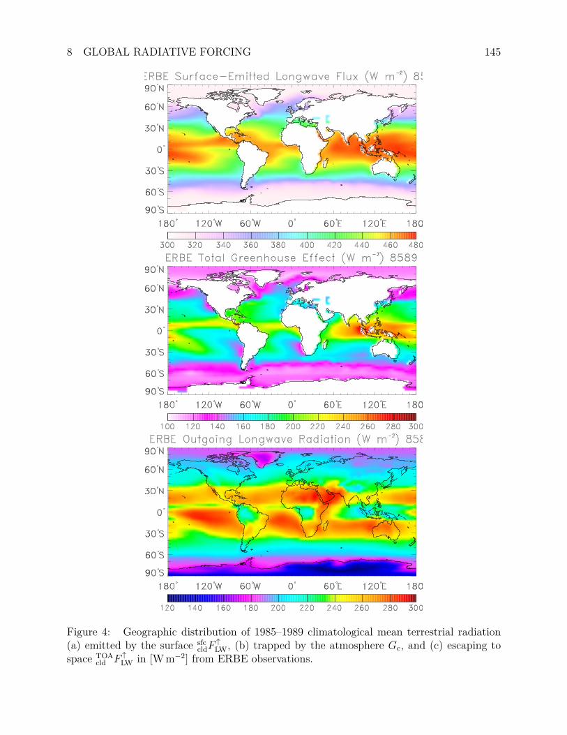
8 GLOBAL RADIATIVE FORCING 145
Figure 4: Geographic distribution of 1985–1989 climatological mean terrestrial radiation(a) emitted by the surface sfc
cldF↑LW, (b) trapped by the atmosphere Gc, and (c) escaping to
space TOAcld F ↑
LW in [W m−2] from ERBE observations.

8 GLOBAL RADIATIVE FORCING 146
Figure 5: Hovmöller diagrams of (a) sea surface temperature [K] and (b) outgoing longwaveradiation [W m−2] over the Equatorial Pacific (averaged 10 S–10 N). Month 1 is January1985. Contour intervals are 0.5 K and 10 W m−2, respectively.
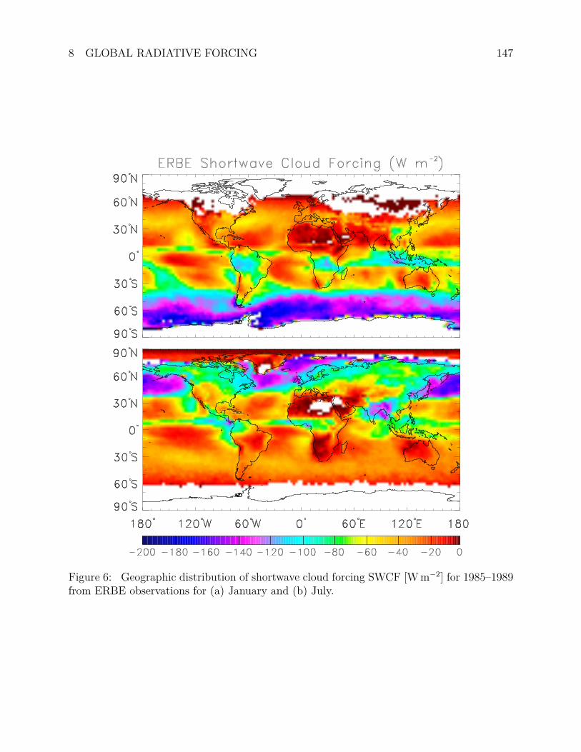
8 GLOBAL RADIATIVE FORCING 147
Figure 6: Geographic distribution of shortwave cloud forcing SWCF [W m−2] for 1985–1989from ERBE observations for (a) January and (b) July.

9 IMPLEMENTATION IN NCAR MODELS 148
Figure 6 shows the shortwave cloud forcing (SWCF) observed by the ERBE satellitesystem from 1985–1989.
Figure 7 shows the zonal mean shortwave cloud forcing (SWCF) observed by the ERBEsatellite system from 1985–1989.
Figure 8 shows the longwave cloud forcing (LWCF) observed by the ERBE satellitesystem from 1985–1989.
Figure 9 shows the zonal mean longwave cloud forcing (LWCF) observed by the ERBEsatellite system from 1985–1989.
Figure 10 shows the balance between solar and terrestrial cloud forcing as observed bythe ERBE satellite system from 1985–1989.
Figure 11 shows the interannual variability of the cloud forcing over the Pacific in termsof Hovmöller diagrams of cloud forcing.
9 Implementation in NCAR modelsThe discussion thus far has centered on the theoretical considerations of radiative transfer.In practice, these ideas must be implemented in computer codes which model, e.g., shortwaveor longwave atmospheric fluxes and heating rates. This section describes how these ideashave been implemented in the NCAR narrow band models.

9 IMPLEMENTATION IN NCAR MODELS 149
Figure 7: Zonal mean shortwave cloud forcing SWCF [W m−2] for 1985–1989 from ERBEobservations and from CCM simulations for (a) January and (b) July.
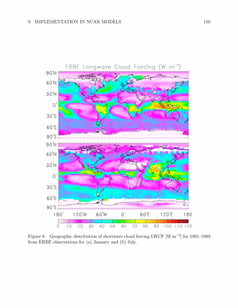
9 IMPLEMENTATION IN NCAR MODELS 150
Figure 8: Geographic distribution of shortwave cloud forcing LWCF [W m−2] for 1985–1989from ERBE observations for (a) January and (b) July.
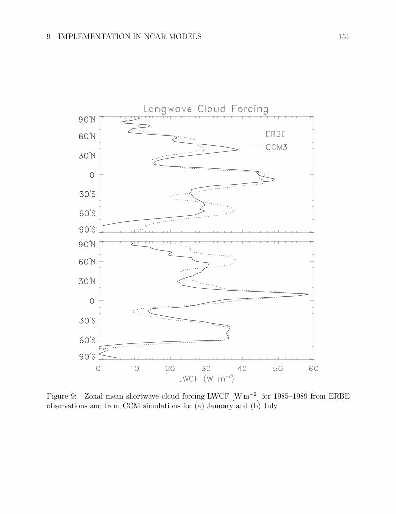
9 IMPLEMENTATION IN NCAR MODELS 151
Figure 9: Zonal mean shortwave cloud forcing LWCF [W m−2] for 1985–1989 from ERBEobservations and from CCM simulations for (a) January and (b) July.

9 IMPLEMENTATION IN NCAR MODELS 152
Figure 10: Geographic distribution of 1985–1989 climatological mean (a) shortwave cloudforcing SWCF, (b) longwave cloud forcing LWCF, and (c) net cloud forcing NCF [W m−2]from ERBE.

9 IMPLEMENTATION IN NCAR MODELS 153
Figure 11: Hovmöller diagrams of cloud forcing [W m−2] in the Equatorial Pacific (averaged10 S–10 N). ERBE observations of (a) shortwave cloud forcing SWCF, and (b) longwavecloud forcing. Month 1 is January 1985. Contour interval is 10 W m−2.

10 APPENDIX 154
10 Appendix
10.1 Vector IdentitiesA number of vector identities are useful in the derivation of Mie theory. For arbitrary vectorsa, b, and c; arbitrary scalars α and β; and scalar fields u = u(x, y, z) and v = v(x, y, z), wehave:
Grad-linearity: ∇(αu+ βv) = α∇u+ β∇v (560a)Div-linearity: ∇ · (αa+ βb) = α∇ · a+ β∇ · b (560b)
Curl-linearity: ∇× (αa+ βb) = α∇× a+ β∇× b (560c)Dot-commutativity: a · b = b · a (560d)
Cross-(non)-commutativity: a× b = −b× a (560e)Scalar Triple Product: a · b× c = c · a× b = b · c× a (560f)
Cross-cross: a× (b× c) = b(a · c)− c(a · b) (560g)(a× b)× c = b(a · c)− a(b · c) (560h)
Curl-cross: ∇× (a× b) = a(∇ · b)− b(∇ · a) + (b · ∇)a− (a · ∇)b (560i)Curl-curl: ∇× (∇× a) = ∇(∇ · a)−∇ · (∇a)
= ∇(∇ · a)−∇2a (560j)Vector Laplacian: ∇2a ≡ (∇ · ∇)a ≡ ∇ · (∇a) (560k)
= ∇(∇ · a)−∇× (∇× a) (560l)Grad-div: ∇(∇ · a) = ∇2a+∇× (∇× a) (560m)
6= (not equal)∇2a
Grad-dot: ∇(a · b) = a× (∇× b) + b× (∇× a) + (b · ∇)a+ (a · ∇)b= (a · ∇)b+ (b · ∇)a+ a× (∇× b) + b× (∇× a)
(560n)Del-vector: ∇a ≡ ∇iiaixi = Dyadic (560o)
Div-grad: ∇ · (∇u) ≡ ∇2u (560p)Div-del: (∇ · ∇)a ≡ ∇2a (560q)
Dot-cross: a · (b× c) = b · (c× a) = c · (a× b) (560r)Div-curl: ∇ · ∇ × a = 0 (560s)Curl-grad: ∇×∇u = 0 (560t)
Div-product: ∇ · (ua) = u∇ · a+ a · ∇u (560u)Curl-product: ∇× (ua) = ∇u× a+ u∇× a (560v)
Dot-del: (a · ∇)a =1
2∇|a|2 + (∇× a)× a (560w)
The divergence of the curl vanishes (560s). The curl of the gradient vanishes (560t).The Laplacian ∇2 is shorthand for (∇ ·∇), and is usually read as “del-squared”, though
it is not the “square” of the del operator. The scalar Laplacian is the divergence of thegradient (560p). However, the vector Laplacian is not the gradient of the divergence (560m).

10 APPENDIX 155
The vector Laplacian ∇2 is defined by (??) which is obtained by simply re-arranging (560j).The vector Laplacian (??) is the gradient of the divergence (560m) minus the curl of the curl(560j).

10 APPENDIX 156
10.2 Legendre PolynomialsThe associated Legendre equation of degree n and order m is
d
dµ
[(1− µ2)
dΘ
dµ
]+
[n(n+ 1)− m2
1− µ2
]Θ = 0 (561)
The solutions to (561) are associated Legendre polynomials, also called spherical harmonics.The associated Legendre polynomial of degree n, order m, and argument µ is denoted byPmn (µ). The Pm
n (µ) are orthogonal functions∫ 1
−1
Pmn (µ)Pm
n′ (µ) dµ = δn,n′2
2n+ 1
(n+m)!
(n−m)!(562)
When m = 0, Pmn (µ) reduces to the Legendre polynomial of order n, Pn(µ) whose orthogo-
nality properties follow from (562) and are shown in (141). Applying suitable normalizationto Pm
n (µ) yields the normalized associated Legendre polynomials Λmn (µ)
Λmn (µ) ≡
√2n+ 1
2
(n−m)!
(n+m)!Pmn (µ) (563)
The Λmn (µ) are orthonormal and are the polar components of the spherical harmonics Y mn (θ, φ)
(566).
10.3 Spherical HarmonicsSpherical harmonics are the product of the normalized associated Legendre polynomials(563) and the orthonormal exponentials (564)
Φm(φ) =1√2π
eimφ (564)
The spherical harmonics Y mn (θ, φ) of degree n and order m are
Y mn (θ, φ) ≡ (−1)m
√2n+ 1
4π
(n−m)!
(n+m)!Pmn (cos θ)eimφ (565)
The Condon-Shortley phase factor (−1)m is a convention which causes the sign alternationfor the positive m spherical harmonics (Arfken, 1985, p. 682).
The spherical harmonics (566) are normalized such that∫ φ=2π
φ=0
∫ θ=π
θ=0
Y m∗n (θ, φ)Y m′
n′ (θ, φ) ≡ δn,n′δm,m′ (566)
where ∗ denotes the complex conjugate.

10 APPENDIX 157
10.4 Bessel FunctionsThe definitive reference for properties of Bessel functions is Watson (1958). Other usefulreferences are Abramowitz and Stegun (1964), p. 374 and Arfken (1985), p. 573. When theHelmholtz equation is solved by separation of variables in cylindrical or spherical coordinates(521), the radial component satisfies Bessel’s equation (Watson, 1958, p. 19),
z2d2w
dz2+ z
dw
dz+ [z2 − ν2]w = 0 (567)
Bessel functions are solutions to (567). The order of the functions is indicated by theparameter ν (not to be confused with frequency). The functions take a single argument z.Both ν and z may be complex, e.g., z = x+ iy, although our particular applications dependonly on real-valued ν. Indeed, we require only integer and half-integer ν.
Due to their power and range of applicability, a menagerie of inter-related solutions to(567) exist. Fortunately, the terminology to identify and describe them is standard. Thestandard Bessel functions of the first kind, second kind, and third kind, are denoted byJν(z), Yν(z), and H
(1)ν (z) and H
(2)ν (z), respectively. Bessel functions of the second kind are
also called Neumann functions and notated with is Nν(z) instead of Yν(z). Mathematicalphysics texts often use the Neumann function notation Nν(z) to avoid confusion with spher-ical harmonics; whereas pure mathematical texts normally use the Yν(z) notation. Besselfunctions of the third kind are also called Hankel functions. All of these satisfy (567) andso are properly called Bessel functions. Specialized versions of Bessel functions derive fromthe three basic kinds. These specializations include modified Bessel functions, and sphericalBessel functions.
General solutions to the Bessel equation (567) are formed from any two linearly indepen-dent Bessel functions. For non-integer ν, Jν(z) and J−ν(z) are linearly independent solutionsand so form a complete basis. However, for integral ν
J−n(z) = (−1)nJn(z) Integer n (568)
and these solutions are not linearly independent.Bessel functions of the second kind Yν(z) are always linearly independent of Jν(z). They
may be defined as
Yν(z) = Nν(z) =Jν(z) cos(νπ)− J−ν(z)
sin νπ(569)
where the RHS limiting value used for integral ν. Bessel functions of the first and secondkind, Jν(z) and Yν(z) together form a complete basis. Series expansion (not shown) revealsthat Yn(z) diverges logarithmically as z → 0. Boundary conditions which require finitesolutions at the origin (z = 0) therefore automatically exclude Yn(z). Conversely, Yn(z) mayappear in any solution which does not require finite values at the origin.
Bessel functions of the third kind (Hankel functions), H(1)ν (z) and H(2)
ν (z), are another setof linearly independent solutions to Bessel’s equation. The relation between these completebases is
H(1)ν (z) = Jν(z) + iYν(z) (570a)
H(2)ν (z) = Jν(z)− iYν(z) (570b)
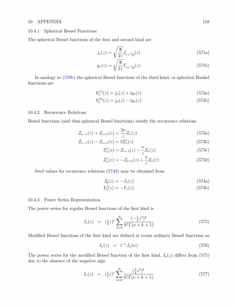
10 APPENDIX 158
10.4.1 Spherical Bessel Functions
The spherical Bessel functions of the first and second kind are
jν(z) =
√π
2zJν+1/2(z) (571a)
yν(z) =
√π
2zYν+1/2(z) (571b)
In analogy to (570b) the spherical Bessel functions of the third kind, or spherical Hankelfunctions are
h(1)ν (z) = jν(z) + iyν(z) (572a)h(2)ν (z) = jν(z)− iyν(z) (572b)
10.4.2 Recurrence Relations
Bessel functions (and thus spherical Bessel functions) satisfy the recurrence relations
Zν−1(z) + Zν+1(z) =2ν
zZν(z) (573a)
Zν−1(z)− Zν+1(z) = 2Z ′ν(z) (573b)
Z ′ν(z) = Zν−1(z)−
ν
zZν(z) (573c)
Z ′ν(z) = −Zν+1(z) +
ν
zZν(z) (573d)
Seed values for recurrence relations (573d) may be obtained from
J ′0(z) = −J1(z) (574a)Y ′0(z) = −Y1(z) (574b)
10.4.3 Power Series Representation
The power series for regular Bessel functions of the first kind is
Jν(z) = (12z)ν
∞∑k=0
(−14z2)k
k! Γ(ν + k + 1)(575)
Modified Bessel functions of the first kind are defined in terms ordinary Bessel functions as
Iν(z) = i−νJν(iz) (576)
The power series for the modified Bessel function of the first kind, Iν(z) differs from (575)due to the absence of the negative sign
Iν(z) = (12z)ν
∞∑k=0
(14z2)k
k! Γ(ν + k + 1)(577)

10 APPENDIX 159
Of particular interest to radiative transfer are I0(z) and I1(z) which appear in the solutionto the mean beam absorptance (397) and equivalent width of an isolated Lorentz line.
I0(z) =∞∑k=0
(12z)2k
(k!)2(578a)
I1(z) =∞∑k=0
(12z)2k+1
k! (k + 1)!(578b)
For z 1, (578) becomes
I0(z 1) ≈ 1 (579a)I1(z 1) ≈ z/2 (579b)
10.4.4 Asymptotic Values
The asymptotic behavior of functions can often be ascertained from their power series rep-resentation. Bessel functions obey the following limits as z → 0:
Zν(z)→ (12z)ν/Γ(ν + 1) (ν 6= −1,−2,−3 . . .) (580a)
Y0(z)→ (2/π) ln z (580b)
Yν(z)→Γ(ν)
π(12z)ν
(580c)
10.5 Gaussian QuadratureThe accuracy of automatic integration of analytic formulae by computers rests on threecriteria:
1. Smoothness of function2. Number of quadrature points3. Placement of quadrature points
For many problems the functional form of the integrand is given. We are usually free tochange, however, the number and placement of quadrature points. For many applications, theoptimal number and location of quadrature points are related through Gaussian quadrature.
Gaussian quadrature points xk have the property that∫ b
a
f(x)w(x) dx ≈n∑k=1
Akf(xk) (581)
is exact if f(x) is any polynomial of degree ≤ 2n − 1. The values of the xk are determinedby the form of the weighting function w(x) and the interval boundaries [a, b]. In fact the xkare the roots of the orthogonal polynomial with weighting function w(x) over the interval[a, b] (see, e.g., Arfken, 1985, p. 969). A common case in radiative transfer has w(x) = 1,[a, b] = [−1, 1] ∫ 1
−1
f(x) dx ≈n∑k=1
Akf(xk) (582)

10 APPENDIX 160
For this case, the xk are the n roots of the Legendre polynomial of degree n, Pn(x), 18 andthe Gaussian weights Ak are defined by the derivative of Pn(x)
xk = x ∈ [0, 1] | Pn(xk) = 0 (583)
Ak =2
(1− x2k)[P ′n(xk)]
2(584)
Radiative transfer problems often use Gaussian weights in the angular integration. De-pending on whether we are concerned with net or hemispherical quantities the angular inte-gration will have different intervals∫ 1
−1
f(x)w(x) dx ≈n∑k=1
Akf(xk) (585)
∫ 1
0
f(y)w(y) dy ≈n∑k=1
Bkf(yk) (586)
Equation (585) is known as full-range Gaussian quadrature and (586) as half-range Gaussianquadrature.
The half-range points and weights are intimately related to the full-range points andweights. The interval y ∈ [0, 1] is a simple linear transformation of x ∈ [−1, 1]
y =x+ 1
2(587)
x = 2y − 1 (588)
The half-range points and weights may be obtained by applying the forward transformation(587) to (585). Thus
yk =xk + 1
2(589)
The weights Ak depend only on n (fxm: I think) and are independent of f(x) and w(x).For Legendre polynomials, the Ak and Bk sum to the size of the interval
n∑k=1
Ak = 2 (590)
n∑k=1
Bk = 1 (591)
A common technique is to apply half of the full range quadrature points and weightsto half of the full range interval, [0, 1]. In this case the quadrature is no longer Gaussian(i.e., not exact for polynomials of degree < 2n), but the quadrature points are often quiteoptimal.
Table 9 lists the first five Legendre polynomials, their roots, the associated full Gaussianangles, and their Gaussian weights. Abramowitz and Stegun (1964), p. 917, list Gaussianquadrature points and weights for n ≤ 32.
Table 10 summarizes the same information needed for half-range Gaussian quadrature.18When w(x) 6= 1, the Gaussian quadrature points are the roots of other orthogonal polynomials, e.g.,
Chebyshev, Laguerre, Hermite.
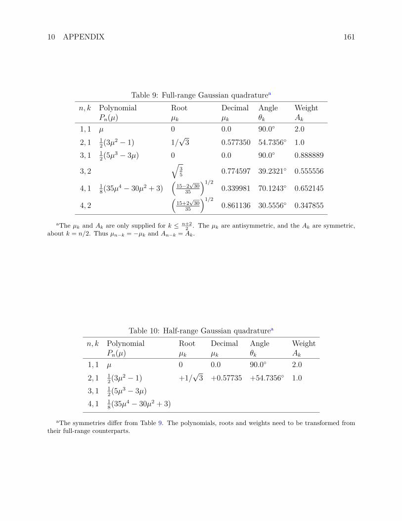
10 APPENDIX 161
Table 9: Full-range Gaussian quadraturea
n, k Polynomial Root Decimal Angle WeightPn(µ) µk µk θk Ak
1, 1 µ 0 0.0 90.0 2.0
2, 1 12(3µ2 − 1) 1/
√3 0.577350 54.7356 1.0
3, 1 12(5µ3 − 3µ) 0 0.0 90.0 0.888889
3, 2√
35
0.774597 39.2321 0.555556
4, 1 18(35µ4 − 30µ2 + 3)
(15−2
√30
35
)1/20.339981 70.1243 0.652145
4, 2(
15+2√30
35
)1/20.861136 30.5556 0.347855
aThe µk and Ak are only supplied for k ≤ n+22 . The µk are antisymmetric, and the Ak are symmetric,
about k = n/2. Thus µn−k = −µk and An−k = Ak.
Table 10: Half-range Gaussian quadraturea
n, k Polynomial Root Decimal Angle WeightPn(µ) µk µk θk Ak
1, 1 µ 0 0.0 90.0 2.02, 1 1
2(3µ2 − 1) +1/
√3 +0.57735 +54.7356 1.0
3, 1 12(5µ3 − 3µ)
4, 1 18(35µ4 − 30µ2 + 3)
aThe symmetries differ from Table 9. The polynomials, roots and weights need to be transformed fromtheir full-range counterparts.

10 APPENDIX 162
10.6 Gauss-Lobatto QuadratureLobatto quadrature, is a type of Gaussian quadrature that prescribes abscissae at the inte-gration endpoints. The Lobatto quadrature rule of order L is∫ +1
−1
f(x) dx =l=L∑l=1
Hlf(xl) (592)
= H1f(−1) +l=L∑l=1
Hlf(xl) +HLf(1) (593)
Whereas Gaussian quadrature is exact for polynomials of degrees ≤ 2L−1, Lobatto quadra-ture fixes two quadrature points and so is exact only for polynomials of degrees ≤ 2L − 3.Nevertheless, the placement of abscissae can give Lobatto quadrature a higher effective accu-racy for certain classes of functions such as asymmetric phase functions (Wiscombe, 1977).
The free (non-prescribed) Lobatto abscissae xl for l = 2, . . . , L− 1 are the L− 2 zeros ofthe derivative of the Legendre polynomial of degree L− 1
P ′L−1(xl) = 0 (594)
(By comparison, the abscissae in Gauss-Legendre quadrature are Legendre polynomial roots).The interior Lobatto weights Hl satisfy
Hl =2
L(L− 1)[PL−1(xl)]2(595)
while the endpoint weights are
H1 = HL =2
L(L− 1)(596)
Michels (1963) describes numerical approaches to determining Lobatto quadrature ab-scissae endpoints and weights. This procedure converges remarkably quickly and smoothly.However, the traditional quadrature variable u = cos(θ) and range [−1, 1] produce abscis-sae that a forward-clustered in cos(θ) and thus angles that are relatively evenly distributed(rather than forward-clustered) in θ.
Wiscombe (1977) puts forward a solution to this problem. He changes the quadraturevariable and domain to θ and [0, π], respectively. Implementing this procedure is relativelystraightforward. The Lobatto weights Hl must be normalized on the new integration domain
Hl =π
L(L− 1)[PL−1(xl)]2(597)
while the endpoint weights are
H1 = HL =π
L(L− 1)(598)

10 APPENDIX 163
10.7 Exponential IntegralsThe exponential integrals En(x) are defined by
En(x) =
∫ ∞
1
t−ne−tx dt (599)
and by the behavior of En(x) at x = 0
E1(0) = ∞En(0) = 1/(n− 1)
A definition equivalent to (599) is obtained by making the change of variable w = t−1. Thismaps t ∈ [1,∞) into w ∈ [1, 0]
w = t−1
t = w−1
dt = −w−2 dw
dw = −t−2 dt (600)
Substituting (600) into (599) we obtain
En(x) =
∫ 0
1
(w−1)−ne−x/w(−w−2) dw
=
∫ 1
0
wnw−2e−x/w dw
=
∫ 1
0
wn−2e−x/w dw (601)
Exponential integrals satisfy two important recurrence relations
−E ′n(x) = −En−1(x) (602a)
nE(n+1)(x) = e−x − xEn(x) (602b)
The angular integral of many radiometric quantities may often be expressed in terms ofthe first few exponential integrals.
En(τ) =
∫ 1
0
µn−2e−τ/µ dµ (603a)
E1(τ) =
∫ 1
0
µ−1e−τ/µ dµ (603b)
E2(τ) =
∫ 1
0
e−τ/µ dµ (603c)
E3(τ) =
∫ 1
0
µe−τ/µ dµ (603d)

BIBLIOGRAPHY 164
BibliographyAbramowitz, M., and I. Stegun (1964), Handbook of Mathematical Functions, 1046 pp.,
Dover, New York. 10.4, 10.5
Arfken, G. (1985), Mathematical Methods for Physicists, third ed., Academic Press, SanDiego, CA. 7.2, 10.3, 10.4, 10.5
Bennett, H. S., and G. J. Rosasco (1978), Resonances in the efficiency factors for absorption:Mie scattering theory, Appl. Opt., 17(4), 491–493. 7.2.7
Bohren, C. F., and D. R. Huffman (1983), Absorption and Scattering of Light by SmallParticles, 530 pp., John Wiley & Sons, New York, NY. 1, 3.3, 7.1, 7.1.1, 7.1.1, 7.1.1, 7.2.1,7.2.2, 7.2.6, 7.2.7
Boucher, O. (1998), On aerosol direct shortwave forcing and the Henyey-Greenstein phasefunction, J. Atmos. Sci., 55(1), 128–134. 2.2.7
Briegleb, B. P. (1992), Longwave band model for thermal radiation in climate studies, J. Geo-phys. Res., 97(D11), 11,475–11,485. 5.5.1, 6.1
Carrier, G. F., M. Krook, and C. E. Pearson (1983), Functions of a Complex Variable, HodBooks, Ithaca, NY. 2.1.11
Cess, R. D. (1985), Nuclear war: Illustrative effects of atmospheric smoke and dust uponsolar radiation, Clim. Change, 7(2), 237–251, doi:10.1007/BF00140,508. 7.5.1
Chang, J. S., R. A. Brost, I. S. A. Isaksen, S. Madronich, P. Middleton, W. R. Stockwell,and C. J. Walcek (1987), A three-dimensional Eulerian acid deposition model: Physicalconcepts and formulation, J. Geophys. Res., 92, 14,681–14,700. 2.1.4
Chou, M. D., and A. Arking (1980), Computation of infrared cooling rates in the watervapor bands, J. Atmos. Sci., 37, 855–867. 6.3.2
Chýlek, P., J. T. Kiehl, and M. K. W. Ko (1978a), Narrow resonance structure in the Miescattering characteristics, Appl. Opt., 17(19), 3019–3021. 7.2.7
Chýlek, P., J. T. Kiehl, and M. K. W. Ko (1978b), Optical levitation and partial-waveresonances, Phys. Rev. A, 18(5), 2229–2233. 7.2.7
Clough, S. A., F. X. Kneizys, and R. W. Davies (1989), Line shape and the water vaporcontinuum, Atmos. Res., 23, 229–241. 5.6.1
Colarco, P. R., O. B. Toon, O. Torres, and P. J. Rasch (2002), Determining the UV imaginaryindex of refraction of Saharan dust particles from Total Ozone Mapping Spectrometerdata using a three-dimensional model of dust transport, J. Geophys. Res., 107(D16),doi:10.1029/2001JD000,903. 7.1
Crisp, D. (1997), Absorption of sunlight in clear and cloudy atmospheres: A solution to thecloud absorption anomaly?, Rejected by J. Geophys. Res. 5.6.1

BIBLIOGRAPHY 165
Dahlback, A., and K. Stamnes (1991), A new spherical model for computing the radiationfield available for photolysis and heating at twilight, Planet. Space Sci., 39(5), 671–683.2.1.4
DeMore, W. B., S. P. Sander, D. M. Golden, R. F. Hampson, M. J. Kurylo, C. J. Howard,A. R. Ravishankara, C. E. Kolb, and M. J. Molina (1994), Chemical kinetics and photo-chemical data for use in stratospheric modeling, Evaluation Number 11 92-20, Jet Propul-sion Laboratory, Pasadena Calif. 4.1.1
Ellingson, R. G., and W. J. Wiscombe (1996), The spectral radiance experiment (SPEC-TRE): Project description and sample results, Bull. Am. Meteorol. Soc., 77(9), 1967–1985.5.6.1
Fu, Q., and K. N. Liou (1992), On the correlated k-distribution method for radiative transferin nonhomogeneous atmospheres, J. Atmos. Sci., 49(22), 2139–2156. 5.6.1
Gamache, R. R., and L. S. Rothman (1992), Extension of the HITRAN database to non-LTEapplications, J. Quant. Spectrosc. Radiat. Transfer, 48(5/6), 519–525. 5.5.1
Gamache, R. R., R. L. Hawkins, and L. S. Rothman (1990), Total internal partition sums inthe temperature range 70–3000 k: atmospheric linear molecules, J. Mol. Spectrosc., 142,205–219. 5.5.1
Gamache, R. R., S. Kennedy, R. L. Hawkins, and L. S. Rothman (2000), Total internalpartition sums for molecules in the terrestrial atmosphere, Journal of Molecular Structure,517/518, 413–431. 5.5.1
Godson, W. L. (1953), The evaluation of infra-red radiative fluxes due to atmospheric watervapour, Q. J. R. Meteorol. Soc., 79, 367–379. 6.2.1
Goody, R. M. (1952), A statistical model for water-vapour absorption, Q. J. R. Meteorol.Soc., 78, 165. 6.2.1
Goody, R. M., and Y. L. Yung (1989), Atmospheric Radiation Theoretical Basis, second ed.,Oxford Univ. Press, New York. 1, 2.2.15, 13, 4.1.5, a, 6.2, 6.3.2
Gradshteyn, I. S., and I. M. Ryzhik (1965), Table of Integrals, Series, and Products, fourthed., Academic Press, New York. 6.2.4
Guimarães, L. G., and H. M. Nussenzveig (1994), Uniform approximation to Mie resonances,J. Modern Optics, 41(3), 625–647. 7.2.7
Hansen, J. E., and L. D. Travis (1974), Light scattering in planetary atmospheres, SpaceSci. Rev., 16, 527–610. 7.2.6
Hess, M., P. Koepke, and I. Schult (1998), Optical properties of aerosols and clouds: Thesoftware package OPAC, Bull. Am. Meteorol. Soc., 79(5), 831–844. 7.1
Hui, A. K., B. H. Armstrong, and A. A. Wray (1978), Rapid computation of the Voigt andcomplex error functions, J. Quant. Spectrosc. Radiat. Transfer, 19, 509–516. 4.1.5
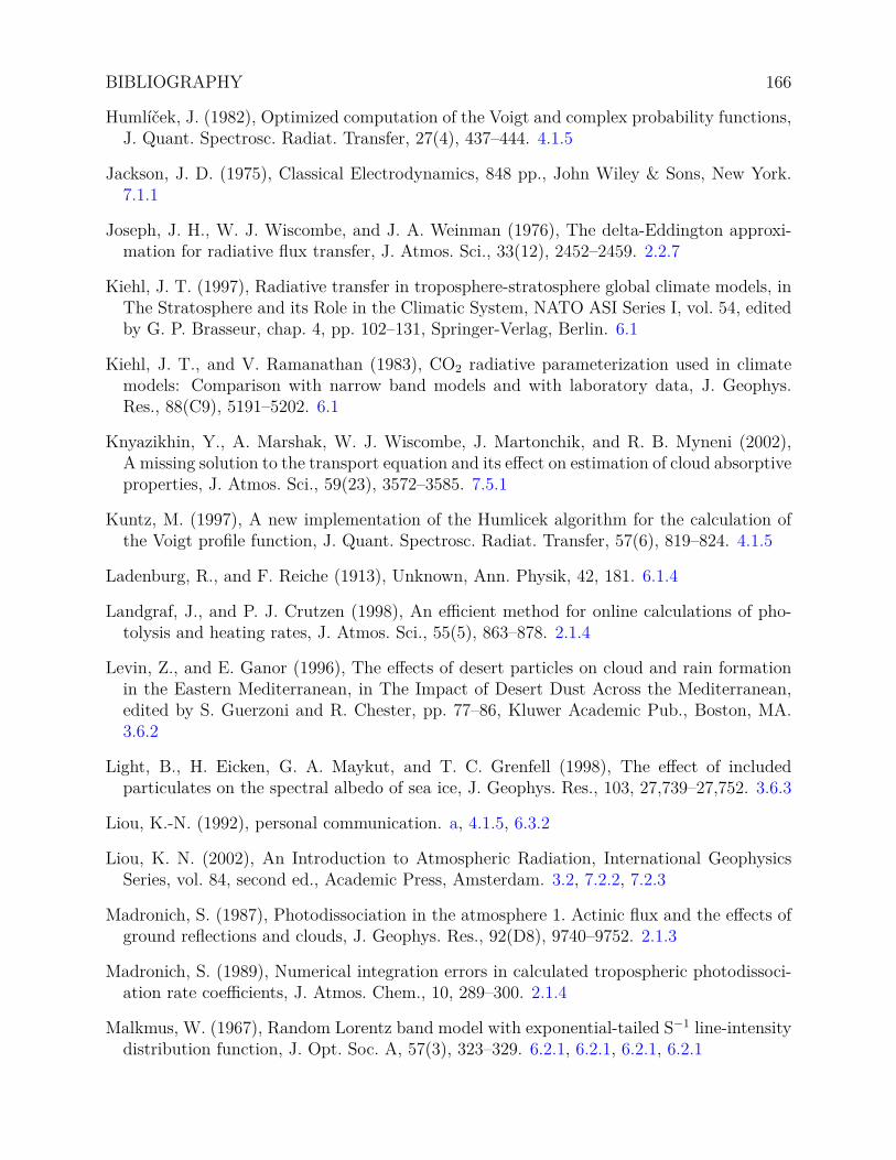
BIBLIOGRAPHY 166
Humlíček, J. (1982), Optimized computation of the Voigt and complex probability functions,J. Quant. Spectrosc. Radiat. Transfer, 27(4), 437–444. 4.1.5
Jackson, J. D. (1975), Classical Electrodynamics, 848 pp., John Wiley & Sons, New York.7.1.1
Joseph, J. H., W. J. Wiscombe, and J. A. Weinman (1976), The delta-Eddington approxi-mation for radiative flux transfer, J. Atmos. Sci., 33(12), 2452–2459. 2.2.7
Kiehl, J. T. (1997), Radiative transfer in troposphere-stratosphere global climate models, inThe Stratosphere and its Role in the Climatic System, NATO ASI Series I, vol. 54, editedby G. P. Brasseur, chap. 4, pp. 102–131, Springer-Verlag, Berlin. 6.1
Kiehl, J. T., and V. Ramanathan (1983), CO2 radiative parameterization used in climatemodels: Comparison with narrow band models and with laboratory data, J. Geophys.Res., 88(C9), 5191–5202. 6.1
Knyazikhin, Y., A. Marshak, W. J. Wiscombe, J. Martonchik, and R. B. Myneni (2002),A missing solution to the transport equation and its effect on estimation of cloud absorptiveproperties, J. Atmos. Sci., 59(23), 3572–3585. 7.5.1
Kuntz, M. (1997), A new implementation of the Humlicek algorithm for the calculation ofthe Voigt profile function, J. Quant. Spectrosc. Radiat. Transfer, 57(6), 819–824. 4.1.5
Ladenburg, R., and F. Reiche (1913), Unknown, Ann. Physik, 42, 181. 6.1.4
Landgraf, J., and P. J. Crutzen (1998), An efficient method for online calculations of pho-tolysis and heating rates, J. Atmos. Sci., 55(5), 863–878. 2.1.4
Levin, Z., and E. Ganor (1996), The effects of desert particles on cloud and rain formationin the Eastern Mediterranean, in The Impact of Desert Dust Across the Mediterranean,edited by S. Guerzoni and R. Chester, pp. 77–86, Kluwer Academic Pub., Boston, MA.3.6.2
Light, B., H. Eicken, G. A. Maykut, and T. C. Grenfell (1998), The effect of includedparticulates on the spectral albedo of sea ice, J. Geophys. Res., 103, 27,739–27,752. 3.6.3
Liou, K.-N. (1992), personal communication. a, 4.1.5, 6.3.2
Liou, K. N. (2002), An Introduction to Atmospheric Radiation, International GeophysicsSeries, vol. 84, second ed., Academic Press, Amsterdam. 3.2, 7.2.2, 7.2.3
Madronich, S. (1987), Photodissociation in the atmosphere 1. Actinic flux and the effects ofground reflections and clouds, J. Geophys. Res., 92(D8), 9740–9752. 2.1.3
Madronich, S. (1989), Numerical integration errors in calculated tropospheric photodissoci-ation rate coefficients, J. Atmos. Chem., 10, 289–300. 2.1.4
Malkmus, W. (1967), Random Lorentz band model with exponential-tailed S−1 line-intensitydistribution function, J. Opt. Soc. A, 57(3), 323–329. 6.2.1, 6.2.1, 6.2.1, 6.2.1

BIBLIOGRAPHY 167
Markel, V. A. (2002), The effects of averaging on the enhancement factor for absorption oflight by carbon particles in microdroplets of water, J. Quant. Spectrosc. Radiat. Transfer,72(6), 765–774. 3.3, 7.2.7
Markel, V. A., and V. M. Shalaev (1999), Absorption of light by soot particles in micro-droplets of water, J. Quant. Spectrosc. Radiat. Transfer, 63(2–6), 321–339, see erratum inJQSRT 66(6):591. 7.2.7
Melnikova, I. (2008), Range of application of the scattering theory within the multi-component turbid media of the cloud atmosphere is the reason for anomalous absorp-tion and incorrectness of climate prediction, Intl. J. Rem. Sens., 29(9), 2615–2628,doi:10.1080/01431160701767,443. 7.5.1
Michels, H. H. (1963), Abscissas and weight coefficients for Lobatto quadrature, Math. Com-put., 17(83), 237–244. 10.6
Mitchell, D. L. (2000), Parameterization of the Mie extinction and absorption coefficientsfor water clouds, J. Atmos. Sci., 57(9), 1311–1326. 7.2.7
Mlawer, E. J., S. J. Taubman, P. D. Brown, M. J. Iacono, and S. A. Clough (1997), Radiativetransfer for inhomogeneous atmospheres: RRTM, a validated correlated-k model for thelongwave, J. Geophys. Res., 102(D14), 16,663–16,682. 5.6.1
Molotch, N. P., T. H. Painter, R. C. Bales, and J. Dozier (2004), Incorporating remotely-sensed snow albedo into a spatially-distributed snowmelt model, Geophys. Res. Lett., 31,L03,501, doi:10.1029/2003GL019,063. 2.3
Moncet, J. L., and S. A. Clough (1997), Accelerated monochromatic radiative transfer forscattering atmospheres: Application of a new model to spectral radiance observations,J. Geophys. Res., 102(D18), 21,853–21,866. 5.6.1
Nussenzveig, H. M. (1992), Diffraction Effects in Semiclassical Scattering, Montroll MemorialLecture Series in Mathematical Physics, vol. 1, Cambridge Univ. Press, Cambridge, UK.3.3
Nussenzveig, H. M. (2003), Light tunneling in clouds, Appl. Opt., 42(9), 1588–1593. 3.3,3.3, 3.3, 3.3, 7.2.7
Partain, P. T., A. K. Heidinger, and G. L. Stephens (2000), High spectral resolution at-mospheric radiative transfer: Application of the equivalence theorem, J. Geophys. Res.,105(D2), 2163–2178. 5.6.1
Patterson, E. M. (1981), Optical properties of the crustal aerosol: Relation to chemical andphysical characteristics, J. Geophys. Res., 86(C4), 3236–3246. 7.1
Patterson, E. M., D. A. Gillette, and B. H. Stockton (1977), Complex index of refractionbetween 300 and 700 nm for Saharan aerosols, J. Geophys. Res., 82(21), 3153–3160. 7.1

BIBLIOGRAPHY 168
Perovich, D. K., and J. W. Govoni (1991), Absorption coefficients of ice from 250 to 400 nm,Geophys. Res. Lett., 18(7), 1233–1235. 7.1
Petropavlovskikh, I. (1995), Evaluation of photodissociation coefficient calculations for usein atmospheric chemical models, Ph.D. thesis, Université Libre de Bruxellex and NationalCenter for Atmospheric Research, Boulder, CO. 2.1.4
Quine, B. M., and J. R. Drummond (2001), GENSPECT: A line-by-line code with selectableinterpolation error tolerance, sub judice, Q. J. R. Meteorol. Soc. 5.6.1
Rees, M. H. (1989), Physics and Chemistry of the Upper Atmosphere, Cambridge Univ.Press, Cambridge. 6.5.1
Rodgers, C. D., and C. D. Walshaw (1966), The computation of infra-red cooling rate inplanetary atmospheres, Q. J. R. Meteorol. Soc., 92(391), 67–92. 6.4
Rogers, R. R., and M. K. Yau (1989), A Short Course in Cloud Physics, 293 pp., PergamonPress, Elmsford, NY. 5.5.1
Rosenfeld, D., Y. Rudich, and R. Lahav (2001), Desert dust suppressing precipitation: A pos-sible desertification feedback loop, Proc. Natl. Acad. Sci., 98, 5975–5980. 3.6.2
Rothman, L. S., et al. (1998), The HITRAN molecular spectroscopic database and HAWKS(HITRAN atmospheric workstations): 1996 edition, J. Quant. Spectrosc. Radiat. Transfer,60(5), 665–710. 4.1.1, a, a, a, 5.3, 5.4, a, 5.5.1, 7.1
Rudich, Y., O. Khersonsky, and D. Rosenfeld (2002), Treating clouds with a grain of salt,Geophys. Res. Lett., 29, doi:10.1029/2002GL016,055. 3.6.2
Salby, M. L. (1996), Fundamentals of Atmospheric Physics, Academic Press, San Diego, CA.2.2.5
Seinfeld, J. H., and S. N. Pandis (1997), Atmospheric Chemistry and Physics, 1326 pp., JohnWiley & Sons, New York, NY. 4.1.3, 4.1.3
Shu, F. H. (1991), The Physics of Astrophysics Volume I: Radiation, University ScienceBooks, Mill Valley, CA. 4.1.2
Sinyuk, A., O. Torres, and O. Dubovik (2003), Combined use of satellite and surface ob-servations to infer the imaginary part of refractive index of Saharan dust, Geophys. Res.Lett., 30(2), 1081, doi:10.1029/2002GL016,189. 7.1
Sparks, L. (1997), Efficient line-by-line calculation of absorption coefficients to high numer-ical accuracy, J. Quant. Spectrosc. Radiat. Transfer, 57(5), 631–650. 5.6.1
Stamnes, K., and S.-C. Tsay (1990), Optimum spectral resolution for computing atmosphericheating and photodissociation rates, Planet. Space Sci., 38(6), 807–820. 2.1.4
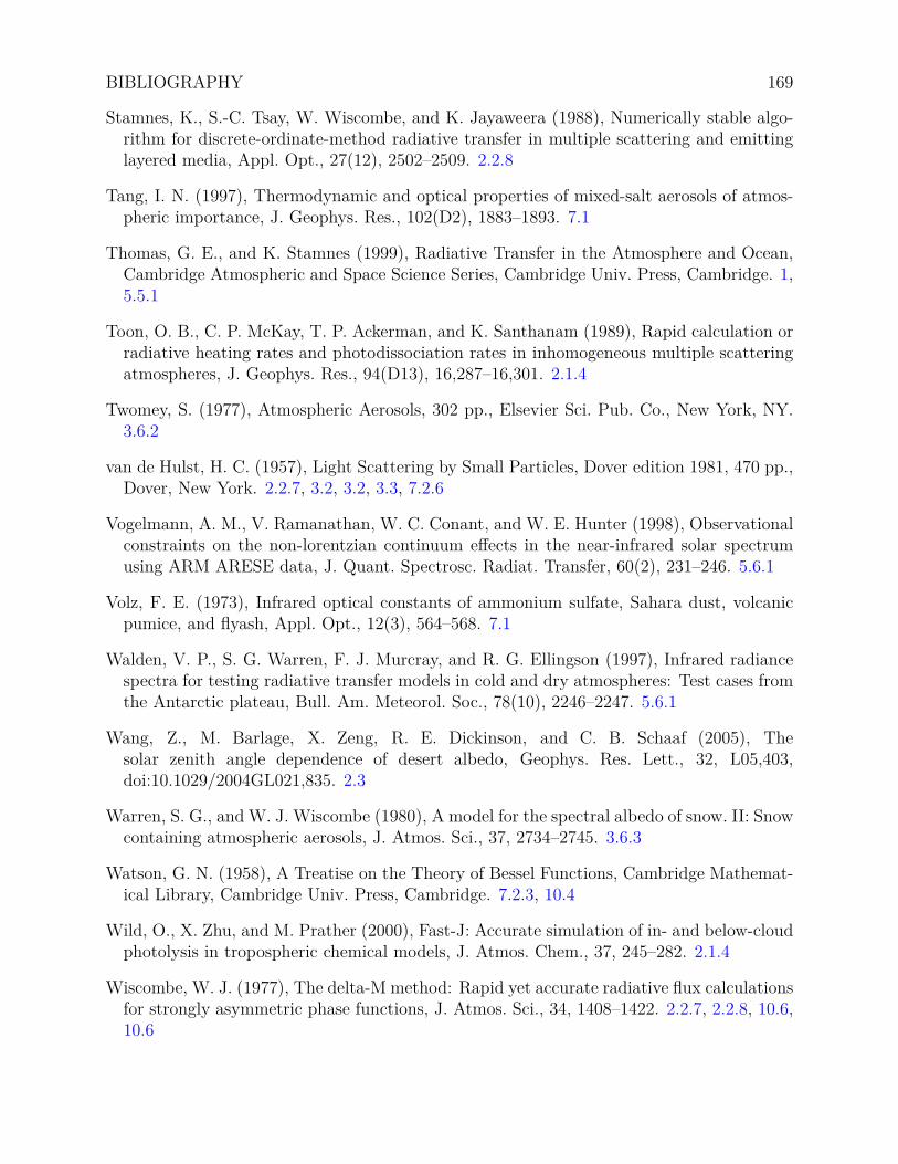
BIBLIOGRAPHY 169
Stamnes, K., S.-C. Tsay, W. Wiscombe, and K. Jayaweera (1988), Numerically stable algo-rithm for discrete-ordinate-method radiative transfer in multiple scattering and emittinglayered media, Appl. Opt., 27(12), 2502–2509. 2.2.8
Tang, I. N. (1997), Thermodynamic and optical properties of mixed-salt aerosols of atmos-pheric importance, J. Geophys. Res., 102(D2), 1883–1893. 7.1
Thomas, G. E., and K. Stamnes (1999), Radiative Transfer in the Atmosphere and Ocean,Cambridge Atmospheric and Space Science Series, Cambridge Univ. Press, Cambridge. 1,5.5.1
Toon, O. B., C. P. McKay, T. P. Ackerman, and K. Santhanam (1989), Rapid calculation orradiative heating rates and photodissociation rates in inhomogeneous multiple scatteringatmospheres, J. Geophys. Res., 94(D13), 16,287–16,301. 2.1.4
Twomey, S. (1977), Atmospheric Aerosols, 302 pp., Elsevier Sci. Pub. Co., New York, NY.3.6.2
van de Hulst, H. C. (1957), Light Scattering by Small Particles, Dover edition 1981, 470 pp.,Dover, New York. 2.2.7, 3.2, 3.2, 3.3, 7.2.6
Vogelmann, A. M., V. Ramanathan, W. C. Conant, and W. E. Hunter (1998), Observationalconstraints on the non-lorentzian continuum effects in the near-infrared solar spectrumusing ARM ARESE data, J. Quant. Spectrosc. Radiat. Transfer, 60(2), 231–246. 5.6.1
Volz, F. E. (1973), Infrared optical constants of ammonium sulfate, Sahara dust, volcanicpumice, and flyash, Appl. Opt., 12(3), 564–568. 7.1
Walden, V. P., S. G. Warren, F. J. Murcray, and R. G. Ellingson (1997), Infrared radiancespectra for testing radiative transfer models in cold and dry atmospheres: Test cases fromthe Antarctic plateau, Bull. Am. Meteorol. Soc., 78(10), 2246–2247. 5.6.1
Wang, Z., M. Barlage, X. Zeng, R. E. Dickinson, and C. B. Schaaf (2005), Thesolar zenith angle dependence of desert albedo, Geophys. Res. Lett., 32, L05,403,doi:10.1029/2004GL021,835. 2.3
Warren, S. G., and W. J. Wiscombe (1980), A model for the spectral albedo of snow. II: Snowcontaining atmospheric aerosols, J. Atmos. Sci., 37, 2734–2745. 3.6.3
Watson, G. N. (1958), A Treatise on the Theory of Bessel Functions, Cambridge Mathemat-ical Library, Cambridge Univ. Press, Cambridge. 7.2.3, 10.4
Wild, O., X. Zhu, and M. Prather (2000), Fast-J: Accurate simulation of in- and below-cloudphotolysis in tropospheric chemical models, J. Atmos. Chem., 37, 245–282. 2.1.4
Wiscombe, W. J. (1977), The delta-M method: Rapid yet accurate radiative flux calculationsfor strongly asymmetric phase functions, J. Atmos. Sci., 34, 1408–1422. 2.2.7, 2.2.8, 10.6,10.6
BIBLIOGRAPHY 170
Wiscombe, W. J. (1979, edited/revised 1996), Mie scattering calculations: Advances in tech-nique and fast, vector-speed computer codes, Tech. Rep. NCAR/TN–140+STR, NationalCenter for Atmospheric Research, Boulder, Colo. 2.2.7
Wiscombe, W. J., and G. W. Grams (1976), The backscattered fraction in two-stream ap-proximations, J. Atmos. Sci., 33(12), 2440–2451. 2.2.7
Wiscombe, W. J., and S. G. Warren (1980), A model for the spectral albedo of snow. I: Puresnow, J. Atmos. Sci., 37, 2712–2733. 3.6.3
Wurzler, S., T. G. Reisin, and Z. Levin (2000), Modification of mineral dust particles by cloudprocessing and subsequent effects on drop size distributions, J. Geophys. Res., 105(D5),4501–4512. 3.6.2
Zender, C. S., and J. Talamantes (2006), Solar absorption by Mie resonancesin cloud droplets, J. Quant. Spectrosc. Radiat. Transfer, 98(1), 122–129,doi:10.1016/j.jqsrt.2005.05.084. 7.2.7
Zender, C. S., B. Bush, S. K. Pope, A. Bucholtz, W. D. Collins, J. T. Kiehl, F. P. J. Valero,and J. Vitko, Jr. (1997), Atmospheric absorption during the Atmospheric Radiation Mea-surement (ARM) Enhanced Shortwave Experiment (ARESE), J. Geophys. Res., 102(D25),29,901–29,915. 6
Indexabs_cff_mss, 141abs_cff_vlm, 141abs_fsh_ffc, 141abs_fsh, 136asm_prm_fsh, 137asm_prm, 142ext_cff_mss, 141ext_cff_vlm, 141ext_fsh_ffc, 141ext_fsh, 136mie, 136, 137, 141, 142sca_cff_mss, 141sca_cff_vlm, 141sca_fsh, 136sct_fsh_ffc, 141ss_alb_fsh, 137ss_alb, 142hitran, 73, 111Ångström exponent, 72Ångström parameter, 72
absorptance, 50absorption, 50absorption cross-section, 9absorption efficiency, 136actinic flux, 8, 15actinic flux enhancement, 11ADT, 65Aerosol Indirect Effects, 71aerosol optical depth, 71air-broadened, 97albedo effect, 71allowed transitions, 86amplitude function, 66analytic, 23angular frequency, 3, 126angular momentum, 85angular velocity, 69anharmonicities, 89anomalous diffraction theory, 65associated Legendre equation, 131, 156asymmetry parameter, 42, 124Avagadro’s number, 96
azimuthal mean operator, 45
back scattering, 39backscattering coefficient, 47backscattering function, 47band absorptance, 100band-integrated, 15basis functions, 130Bessel functions, 102, 133, 157Bessel functions of the second kind, 157Bessel functions of the third kind, 157Bessel functions, modified, 133, 158Bessel’s equation, 132, 133, 157bidirectional reflectance distribution function,
52blackbody radiation, 16Boltzmann statistics, 90Boltzmann’s Law, 91Bond albedo, 54bond strength, 87BRDF, 45brightness temperature, 65broadband, 15bulk single scattering properties, 142
C-G approximation, 122CAM, 68, 140carbon monoxide, 88centripetal acceleration, 70Chapman function, 124classical value, 79cloud glaciation effect, 71cloud lifetime effect, 71collimated, 11, 27Collision broadening, 83collision broadening, 72combination bands, 90complex angular momentum, 68complex conjugate, 156complex error function, 83complex permittivity, 126complex plane wave, 126Condon-Shortley, 156conductivity, 125
171

INDEX 172
constitutive equations, 125, 126cooling rate, 37cross-section, 9curve of growth, 101
diatomic molecules, 87diffuse component, 42diffusivity approximation, 49diffusivity factor, 35, 49, 118dipole approximation, 93dipole moment, 84direct component, 42directional reflectance, 54DISORT, 41Doppler broadening, 72, 81, 83Doppler line shape, 81, 82Doppler width, 82downwelling, 20droplet size effect, 71
effective asymmetry parameter, 140effective single scattering properties, 138, 140effective temperature, 2, 25electric displacement, 125electric field, 125, 135electric polarization, 125electric susceptibility, 125electron rest mass, 94electronic energy, 84emission, 25energy, 3energy density, 15equation of radiative transfer, 26equivalance theorem, 98equivalent width, 100expansion coefficients, 41exponential integrals, 34, 163exponential line strength distribution, 104extinction, 25extinction coefficient, 25extinction efficiency, 136extinction law, 28, 104extinction optical depth, 124
field of view, 6flux absorptance, total, 61
flux reflectance, 53, 54flux reflectance, total, 61flux transmission, 55flux transmissivity, 34flux transmittance, total, 61forbidden transitions, 86foreign-broadened, 97forward scattering, 39forward scattering function, 47free charge density, 125free current density, 125frequency, 2frequency of maximum emission, 18full Gaussian quadrature, 49full-range Gaussian quadrature, 160fundamental transition, 89
Gamma function, 22, 23gamma function, 103, 106gauge transformation, 127Gauss-Lobatto, 41Gaussian distribution, 83Gaussian quadrature, 159, 162Gaussian weights, 160GCMs, 140generating function, 127geometric optics approximation, 68global solar pyranometers, 71GOA, 68Goody distribution, 104greenhouse effect, 2, 36grey atmosphere, 36
H-C-G approximation, 120, 122half-range fluxes, 20half-range Gaussian quadrature, 160half-range intensities, 7, 30, 42Hankel functions, 157harmonic coupling bands, 90heating rate, 37Helmholtz equation, 129, 157hemispheric, 19hemispheric fluxes, 20hemispheric intensities, 7, 19hemispheric intensity, 46
INDEX 173
Henyey-Greenstein Phase Function, 41homogeneous, 5, 126homonuclear, 84hydrostatic equilibrium, 119
impaction parameter, 65incident plane wave, 133incident wave, 134independent scatterers, 142index of refraction, 124induced emission, 94integrating factor, 31integration by parts, 67irradiance, 2isotropic, 5, 11, 126isotropic radiation, 6isotropic scattering, 39
Kepler’s Law, 70kinetic collisions, 77
Ladenburg and Reiche function, 102Lambertian surface, 11, 52, 54Laplacian, 128layer single scattering properties, 142Legendre polynomial, 156, 160Legendre polynomials, 40, 131line intensity, 73line shape factor, 73line strength, 73, 93–95line strength distribution function, 104line width exponent, 79line-by-line, 56, 99line-by-line models, 140linear, 126liquid water content, 64liquid water path, 64Lobatto quadrature, 162local thermodynamic equilibrium, 16Lorentz broadening, 81Lorentz line shape, 74Lorentz line width, 81Lorenz-Mie, 134LTE, 98luminosity, 24LWC effect, 71
macroscopic, 125magnetic field, 125magnetic induction, 125magnetization, 125mass absorption coefficient, 74, 138matrix element, 93Maxwell distribution, 76Maxwell equations, 126Maxwell’s equations, 65, 125Maxwell-Boltzmann statistics, 77mean effective asymmetry parameter, 142mean effective efficiencies, 141mean effective single scattering properties, 140mean free path, 77mean intensity, 5mean line intensity, 108, 108, 109mean transmittance, 99mhos, 125mid-latitude summer, 12Mie theory, 65, 134MODIS, 52molecular cross section, 9moment of inertia, 85monochromatic beam absorptance, 100monodisperse, 138multiplication property, 118
narrow band models, 98narrowband, 15natural line shape, 74Natural line width, 72Neumann, 157Newton’s Second Law, 70nonlocal thermodynamic equilibrium, 98normal incidence pyrheliometer, 71nuclear energy, 84number absorption coefficient, 72, 74
optical collisions, 77optical cross section, 80optical depth, 5, 26optical efficiencies, 136optical path, 26orbital period, 69orthogonal functions, 156
INDEX 174
orthonormal, 41, 130, 156oscillator strength, 94overtone bands, 90
P-branch, 90particle wave, 134permeability, 125permeability of free space, 125permittivity of free space, 125phase function, 39, 40, 46phase function moments, 41phase lag, 66phenomenological coefficients, 126photo-absorption, 8photolysis cutoff frequency, 9photolysis rate, 11photolysis rate coefficient, 9, 10photosphere, 25Planck weighting, 140Planck’s constant, 3plane albedo, 53plane-parallel, 5planetary albedo, 2, 54planetary radiative equilibrium, 2, 16Poisson distribution, 76, 77power series, 22, 22, 158pressure broadening, 72, 76pressure-broadened line width, 76pressure-shift, 97
quantum efficiency, 9quantum yield, 9
R-branch, 90radiance, 4radiative equilibrium, 37radiative equilibrium temperature profile, 36radiative flux divergence, 37radius of curvature, 124random band, 119Rayleigh limit, 64Rayleigh weighting, 140Rayleigh-Jeans limit, 18reciprocity relations, 47reduced mass, 85reflectance, 11, 50
reflection, 50residue theorem, 24resonances, 135resonant absorption, 135Riemann zeta function, 21, 22rigid rotator, 84rotational constant, 86rotational energy, 84rotational partition function, 91rotational quantum number, 85
scaled absorber path, 120scaled pressure, 120scaled temperature, 120scaling approximation, 120scattered wave, 134scattering, 39scattering angle, 39, 66scattering efficiency, 136selection rule, 86selection rules, 89self-broadening, 97separation constant, 129separation of variables, 129shaded pyranometers, 71shadowband radiometers, 71single scattering albedo, 124single scattering properties, 124single-scattering approximation, 69single-scattering source function, 45, 46, 69size parameter, 64size parameters, 65solar constant, 2, 25solid angle, 3source function, 26specific extinction, 139specific heat capacity at constant pressure, 37specific intensity, 4spectral, 15spectral absorption cross section, 72spectroscopy, 84specular, 42speed of light, 3spherical albedo, 2, 54spherical Bessel function, 135

INDEX 175
spherical Bessel functions, 158spherical Hankel functions, 158spherical harmonics, 156spherical polar coordinates, 6, 39spontaneous decay, 74spontaneous emission, 74, 93spring constant, 87statistical weight, 90Stefan-Boltzmann constant, 24Stefan-Boltzmann Law, 2, 24, 35stimulated absorption, 94stimulated emission, 94stratified atmosphere, 5, 29strong line limit, 103, 104strong-line limit, 103surface reflectance, 30, 44, 52, 140SWNB2, 140
Tesla, 125the mass extinction coefficient, 25the number extinction coefficient, 25the volume extinction coefficient, 25thermal emission, 16thermal speed, 77thermodynamic equilibrium, 16TOA, 38tranlational kinetic energy, 84transmission, 50transmittance, 50, 50two level atom, 93two stream equations, 46two-stream approximation, 35, 56
upwelling, 20
vector identities, 154vector spherical harmonic, 135vector wave equation, 127, 128vibration-rotation bands, 90vibrational constant, 88vibrational energy, 84vibrational ground state, 89vibrational partition function, 91vibrational quantum number, 88Voigt line shape, 72Voigt profile, 83
volume absorption coefficient, 72volume extinction coefficient, 28
warming rate, 37wavelength, 3wavenumber, 3, 3, 127weak-line limit, 102Wentzel-Kramers-Brillouin, 68Wien’s Displacement Law, 19Wien’s limit, 17WKB, 68
zero-point energy, 89, 92