R. Bhar, A. G. Malliaris Deviation of US Equity Return Are They Determined by Fundamental or...
31
R. Bhar, A. G. Mall iaris www.bhar.id.au 1 Deviation of US Equity Return Are They Determined by Fundamental or Behavioral Variables? R. Bhar (UNSW), A. G. Malliaris (Loyola, Chicago)
-
Upload
kathleen-kelly -
Category
Documents
-
view
216 -
download
1
Transcript of R. Bhar, A. G. Malliaris Deviation of US Equity Return Are They Determined by Fundamental or...
R. Bhar, A. G. Malliaris www.bhar.id.au 1
Deviation of US Equity Return
Are They Determined by Fundamental or Behavioral Variables?
R. Bhar (UNSW), A. G. Malliaris (Loyola, Chicago)
R. Bhar, A. G. Malliaris www.bhar.id.au 2
Background
Focus is on the intersection of financial markets and macro-economics
Cochrane (2006) is a brilliant survey of this area
Indicates long-run averages of GDP, dividend, equity – mostly with annual data
R. Bhar, A. G. Malliaris www.bhar.id.au 3
Background
On a year by year basis deviations from long-run averages do not seem high
FRB St Louis (June 2007) shows S&P 500 return: Stable (’92-’94) Very high (’82-’83, ’97-’98)
R. Bhar, A. G. Malliaris www.bhar.id.au 4
Recent Literature
Economists at FRB St Louis assert stock market boom takes place during above average GDP growth and below average inflation
They don’t find evidence of liquidity as a factor

R. Bhar, A. G. Malliaris www.bhar.id.au 5
Recent Literature
Rapid economic growth increases corporate profitability that in turn leads to above normal increases in stock prices
Stock market boom reflects real positive macro fundamentals and monetary policy targeting price stability

R. Bhar, A. G. Malliaris www.bhar.id.au 6
Recent Literature
A strong economy growing without concern for inflation most often induce stock price boom
They also find stock market boom ends within a few months of an increase in inflation
R. Bhar, A. G. Malliaris www.bhar.id.au 7
Recent Literature
In addition to economic fundamentals, behavioral finance has offered valuable explanations for several asset pricing puzzles
Momentum return concept in the aggregate market refers broadly to continuation of short-term return
R. Bhar, A. G. Malliaris www.bhar.id.au 8
Recent Literature
Barberis and Thaler (2005) suggest momentum return in the aggregate market in the form of persistence of above average return during periods of boom can be an important behavioral variable
R. Bhar, A. G. Malliaris www.bhar.id.au 9
Aim & Hypothesis
Based on this literature review, we attempt to explain deviations of equity return from long-term average with the help of both fundamental and behavioral variables
Aim is to explain post WW II era Use important macro-economic variables: inflation, funds
rate and unemployment Also, use behavioral variable – momentum return
R. Bhar, A. G. Malliaris www.bhar.id.au 10
Data & Model
We use monthly data covering the period June 1965 to November 2005
All economic data obtained from FRB St Louis website
S&P data obtained from DataStream We use inverse unemployment rate as
suggested in Ferrara (2003)
R. Bhar, A. G. Malliaris www.bhar.id.au 11
Data & Model
Deviation from long-term average is computed as the difference between current return and the last eight months moving average
In order to understand the behavior of the variables we first tried a linear regression

R. Bhar, A. G. Malliaris www.bhar.id.au 12
Data & Model
Linear regression
We use first differences of funds rate and inverse unemployment rate – these are non-stationary
t 0 1 t 2 t 1 3 t
4 t 1 5 t 6 t 1
xsr inf inf fnd
fnd ium ium

R. Bhar, A. G. Malliaris www.bhar.id.au 13
Regression Results
In linear regression not significant
Only and are significant R-square only 6% Residual CUSUM square test shows
parameter and/or variance instability
t 1inf t 1fnd
t 1xsr
R. Bhar, A. G. Malliaris www.bhar.id.au 14
Regression Results
Linear model like this one simply captures the average effect
We need to account for structural instability in a meaningful way
Some of the insignificant parameters may be important during some ‘states’
R. Bhar, A. G. Malliaris www.bhar.id.au 15
Markov Switching Model
How do we define ‘states? A popular approach in economic
analysis is to let an unobserved Markov chain to drive transition between states
Question: How many states? What is the probability of transition?
R. Bhar, A. G. Malliaris www.bhar.id.au 16
Markov Switching Model
We resort to the business cycle literature to decide on the number of states
Ferrara (2003) suggests three states for the US economy
Statistical alternative to this may not be computationally feasible
R. Bhar, A. G. Malliaris www.bhar.id.au 17
Markov Switching Model
Transition probability between states inferred from the data
Computational complexity of such models is well known
We use maximum likelihood method together with Expectation Maximization (EM) algorithm
R. Bhar, A. G. Malliaris www.bhar.id.au 18
Markov Switching Model
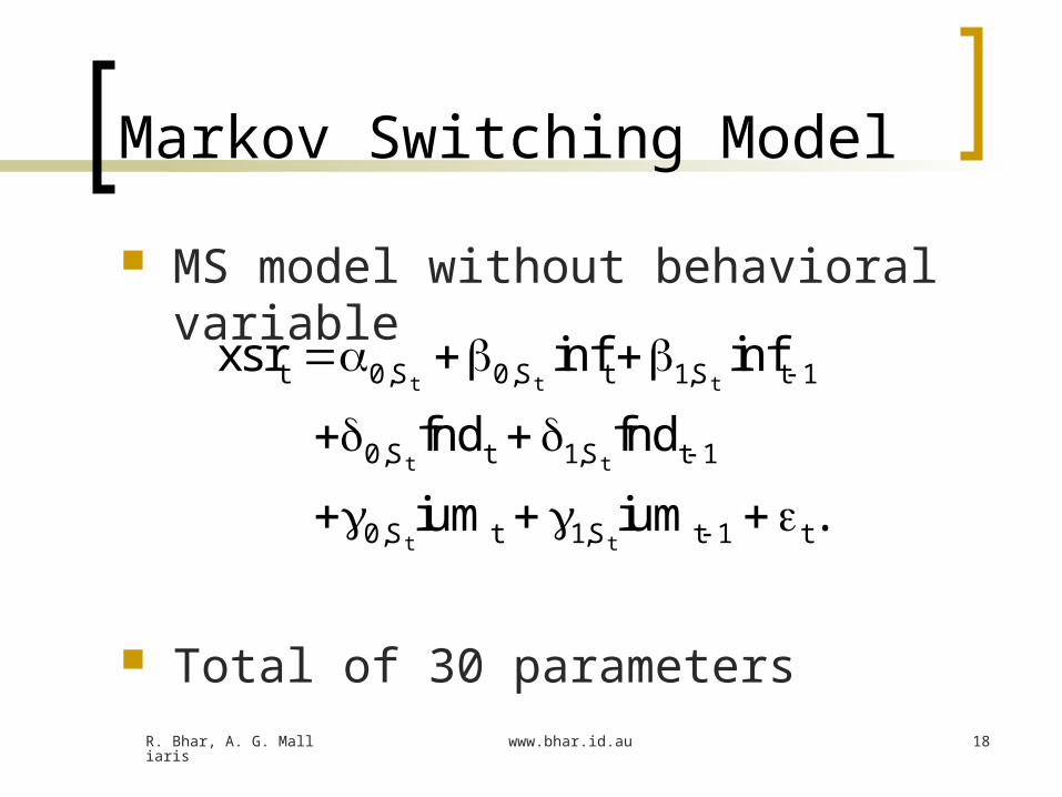
MS model without behavioral variable
Total of 30 parameters
t t t
t t
t t
t 0,S 0,S t 1,S t 1
0,S t 1,S t 1
0,S t 1,S t 1 t
xsr inf inf
fnd fnd
ium ium .

R. Bhar, A. G. Malliaris www.bhar.id.au 19
Markov Switching Model
Let us first look at the model inferred plots of the probability of being in a state for each month in the data (Figure 1)
A quick look at the estimation results (Table 1)
R. Bhar, A. G. Malliaris www.bhar.id.au 20
Markov Switching Model
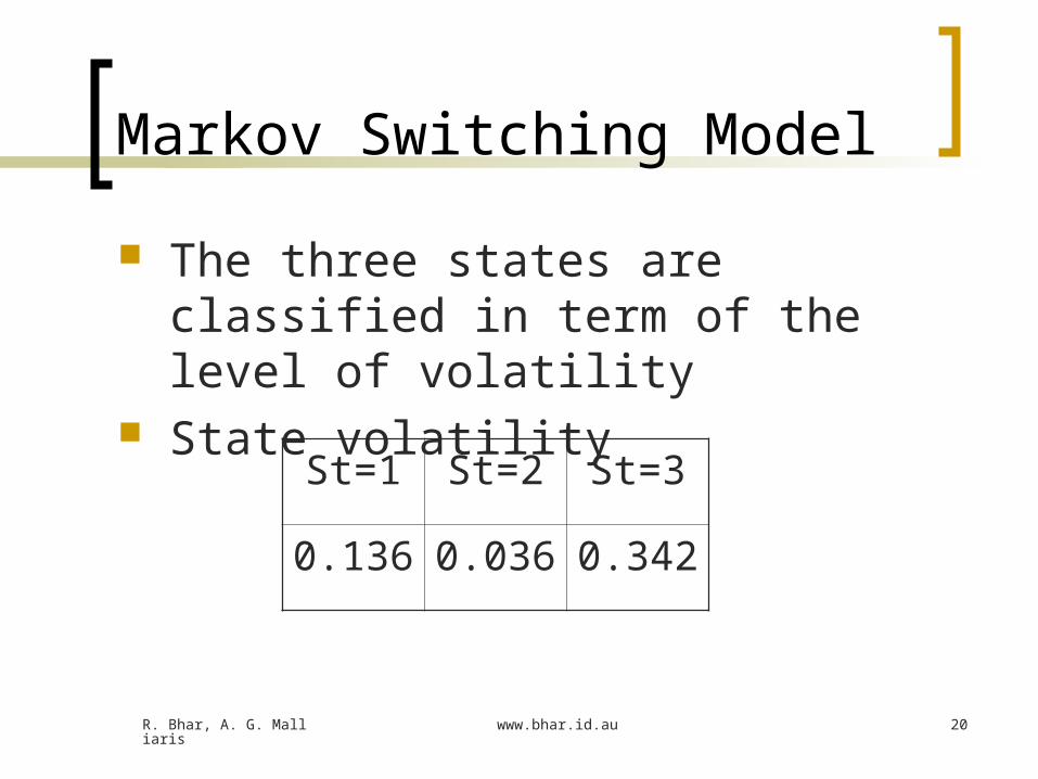
The three states are classified in term of the level of volatility
State volatility
St=1 St=2 St=3
0.136 0.036 0.342

R. Bhar, A. G. Malliaris www.bhar.id.au 21
Markov Switching Model
Transition probability
0.976 0.393 0.044
0.023 0.926 0.077
0.000 0.033 0.877
R. Bhar, A. G. Malliaris www.bhar.id.au 22
Markov Switching Model
Linear regression model did not find inflation significant
In the MS model inflation is significant for St=1 and 2
State St=2 is particularly interesting It has the lowest volatility Positive average deviation in return
R. Bhar, A. G. Malliaris www.bhar.id.au 23
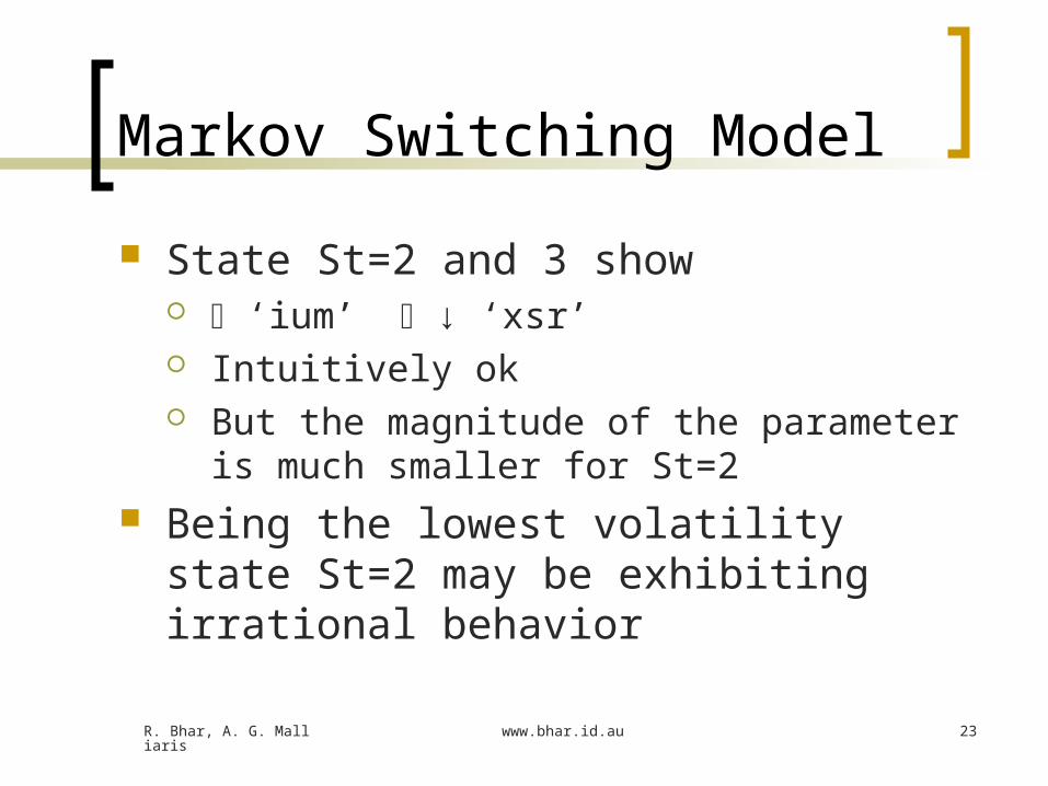
Markov Switching Model
State St=2 and 3 show ‘ium’ ↓ ‘xsr’ Intuitively ok But the magnitude of the parameter is
much smaller for St=2 Being the lowest volatility state St=2
may be exhibiting irrational behavior
R. Bhar, A. G. Malliaris www.bhar.id.au 24
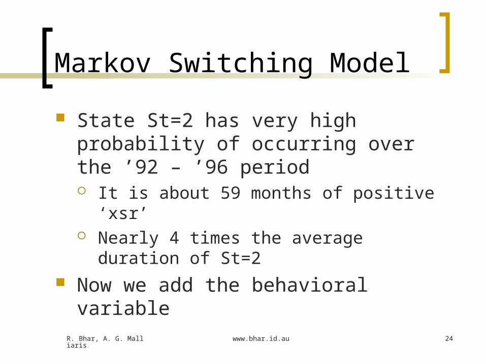
Markov Switching Model
State St=2 has very high probability of occurring over the ’92 – ’96 period It is about 59 months of positive ‘xsr’ Nearly 4 times the average duration of
St=2 Now we add the behavioral variable
R. Bhar, A. G. Malliaris www.bhar.id.au 25
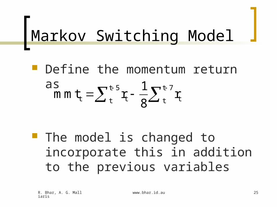
Markov Switching Model
Define the momentum return as
The model is changed to incorporate this in addition to the previous variables
t 5 t 7
t t tt t
1mmt r r
8
R. Bhar, A. G. Malliaris www.bhar.id.au 26
Markov Switching Model
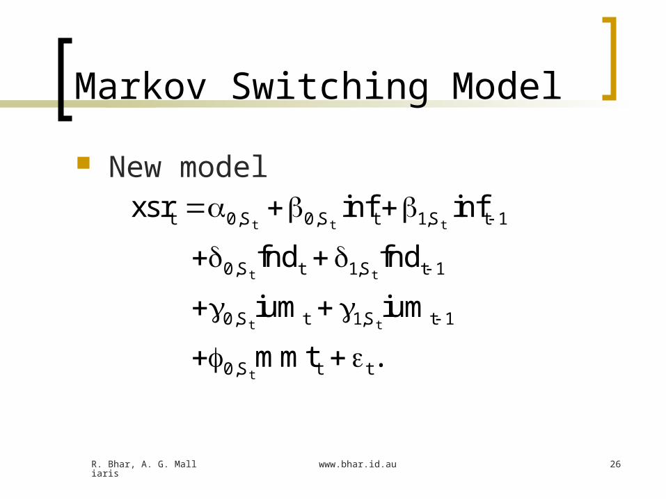
New model
t t t
t t
t t
t
t 0,S 0,S t 1,S t 1
0,S t 1,S t 1
0,S t 1,S t 1
0,S t t
xsr inf inf
fnd fnd
ium ium
mmt .

R. Bhar, A. G. Malliaris www.bhar.id.au 27
Markov Switching Model
New probability of states (Figure 2) There are now 33 parameters and a
quick look at the estimation results (Table 2)
Estimation results are similar to that in the previous model
R. Bhar, A. G. Malliaris www.bhar.id.au 28
Markov Switching Model
Average positive ‘xsr’ in St=2 is nearly twice as much in the pervious model
St=2 has still the lowest volatility ‘mmt’ parameter only significant for
St=1 and 2 Increasing ‘mmt’ reduces available ‘xsr’
R. Bhar, A. G. Malliaris www.bhar.id.au 29
Markov Switching Model
St=3 captures the most volatile periods of ’70s, ’80s and early 2000 Has the shortest expected duration (7-8
months)
R. Bhar, A. G. Malliaris www.bhar.id.au 30
Conclusions
Extensive statistical diagnostics prove the efficacy of the MS approach
Incremental explanatory power of the model with ‘mmt’ has been proved by Vuong (1989) statistic Conclusively proves the influence of the
behavioral variable for ‘xsr’
R. Bhar, A. G. Malliaris www.bhar.id.au 31
Conclusions
Markov regime based model brings out better understanding of the nature of interaction between return deviation from long-run average and macro-economic and behavioral variables


![[Ramaprasad Bhar] Stochastic Filtering With Applic(Bookos.org)](https://static.fdocuments.in/doc/165x107/577cca1c1a28aba711a564dd/ramaprasad-bhar-stochastic-filtering-with-applicbookosorg.jpg)