Queueing Theory Dr. Antonio A. Trani CEE 5614 Analysis of Air Transportation Systems...
137
Virginia Tech (A.A. Trani) Queueing Theory Dr. Antonio A. Trani CEE 5614 Analysis of Air Transportation Systems Fall 2012
Transcript of Queueing Theory Dr. Antonio A. Trani CEE 5614 Analysis of Air Transportation Systems...

Virginia Tech (A.A. Trani)
Queueing Theory
Dr. Antonio A. Trani
CEE 5614Analysis of Air Transportation Systems
Fall 2012

Virginia Polytechnic Institute and State University
2 of 95
Material Presented in this Section
The importance of queueing models in infrastructure planning and design cannot be overstated.
Queueing models offer a simplified way to analyze critical areas inside an airport terminal to evaluate levels of service and operational performance.
Topics
Queueing Models+ Background + Analytic solutions for various disciplines+ Applications to infrastructure planning

Virginia Polytechnic Institute and State University
3 of 95
Principles of Queueing Theory
Historically starts with the work of A.K. Erlang while estimating queues for telephone systems
Applications are very numerous:
•
Transportation planning (vehicle delays in networks)
•
Public health facility design (emergency rooms)
•
Commerce and industry (waiting line analysis)
•
Communications infrastructure (switches and lines)

Virginia Polytechnic Institute and State University
4 of 95
Elements of a Queue
a) Input Source
b) Queue
c) Service facility
Arriving EntitiesServed Entities
Service facility
Queue
Queueing SystemInput Source

Virginia Polytechnic Institute and State University
5 of 95
Specification of a Queue
•
Size of input source
•
Input function
•
Queue discipline
•
Service discipline
•
Service facility configuration
•
Output function (distribution of service times)
Sample queue disciplines
•
FIFO - first in, first out
•
Time-based disciplines
•
Priority discipline

Virginia Polytechnic Institute and State University
6 of 95
What Does a Queue Represent?
Queues represent the state of a system such as the number of people inside an airport terminal, the number of trucks waiting to be loaded at a construction site, the number of ships waiting to be unloaded in a dock, the number of aircraft holding in an imaginary racetrack flight pattern near an airport facility, etc.
The important feature seems to be that the analysis is common to many realistic situations where a flows of traffic (including pedestrians movind inside airport terminals) can be described in terms of either continuous flows or discrete events.

Virginia Polytechnic Institute and State University
7 of 95
Types of Queues
Deterministic queues
- Values of arrival funtion are not random variables (continuous flow) but do vary over time.
• Example of this process is the hydrodynamic approximation of pedestrian flows inside airport terminals
• “Bottleneck” analysis in transportation processes employs this technique
Stochastic queues
- deal with random variables for arrival and service time functions.
• Queues are defined by probabilistic metrics such as the expected number of entities in the system, probability of
n
entities in the system and so on

Virginia Polytechnic Institute and State University
8 of 95
Generalized Time Behavior of a Queue
The state of the system goes through two well defined regions of behavior: a) transient and b) steady-state
Time (hrs)
Stateof System
Transient Behavior
Steady-State

Virginia Polytechnic Institute and State University
9 of 95
Deterministic Queues
Deterministic Queues are analogous to a continuous flow of entities passing over a point over time. As Morlok [Morlok, 1976] points out this type of analysis is usually carried out when the number of entities to be simulated is large as this will ensure a better match between the resulting cumulative stepped line representing the state of the system and the continuous approximation line
The figure below depicts graphically a deterministic queue characterized by a region where demand exceeds supply for a period of time

Virginia Polytechnic Institute and State University
10 of 95
Deterministic Queues (Continuous)
Demand
SupplyRates
Cumulative Flow
Cumulative Supply
CumulativeDemand
Supply Deficit
Time
Lt
Wt
tin tout

Virginia Polytechnic Institute and State University
11 of 95
Deterministic Queues (Discrete Case)
Demand (λ)
Supply (µ)Rates
Cumulative Flow
Cumulative Supply
CumulativeDemand
Supply Deficit
Time∆t

Virginia Polytechnic Institute and State University
12 of 95
Deterministic Queues (Parameters)
a) The queue length, , (i.e., state of the system) corresponds to the maximum ordinate distance between the cumulative demand and supply curves
b) The waiting time, , denoted by the horizontal distance between the two cumulative curves in the diagram is the individual waiting time of an entity arriving to the queue at time
c) The total delay is the area under bounded by these two curves
d) The average delay time is the quotient of the total delay and the number of entities processed
Lt
Wt
tin

Virginia Polytechnic Institute and State University
13 of 95
Deterministic Queues
e) The average queue length is the quotient of the total delay and the time span of the delay (i.e., the time difference between the end and start of the delay)
Assumptions
Demand and supply curves are derived derived from known flow rate functions (
λ
and
µ
) which of course are functions of time.
The diagrams shown represent a simplified scenario arising in many practical situations such as those encountered in traffic engineering (i.e., bottleneck analysis).

Virginia Tech (A.A. Trani)
Fundamental EquationsDeterministic Queueing
13a of 95

Virginia Polytechnic Institute and State University
14 of 95
Example : Freeway Bottleneck Analysis
A four lane freeway has a total directional demand of 4,000 veh/hr during the morning peak period. One day an accident occurs at the freeway that blocks the right-hand side lane for 30 minutes (at time t=1.0 hours). The capacity per lane is 2,200 veh/hr.
a) Find the maximum number of cars queued.
b) Find the average delay imposed to all cars during the queue.
Virginia Tech (A.A. Trani)
Mathematical Equations to Work the Problem
λ(t) = 4000 ∀ t
µ(t) =4400 if t < 1.0 hrs
2200 if 1 <= t < 1.5 hrs4400 if t > 1.5 hrs
dLdt
= λ(t)− µ(t)
In finite difference form we can solve the equationfor Lt numerically
Lt = Lt−Δt +dLdt
⎛⎝⎜
⎞⎠⎟ Δt
Lt = Lt−Δt + λ(t)− µ(t)( )Δt
First-order differential equation to be solved
14a of 95

Virginia Tech (A.A. Trani)
Hand Calculations and Solution
• Integrate the values of demand and capacity in a piecewise fashion (over time)
• For example for interval 0 < t <1.0 hrs
14b of 95

Virginia Tech (A.A. Trani)
Hand Calculations and Solution
• For interval 1.0 <= t <1.5 hrs
14c of 95
Virginia Tech (A.A. Trani)
Hand Calculations and Solution
• For interval 1.5 <= t <3.75 hrs
14d of 95

Virginia Tech (A.A. Trani)
Cumulative Flow Diagram(Integral of demand and supply functions)
red = cumulative demandblue = cumulative supply
14e of 95

Virginia Tech (A.A. Trani)
Excel Numerical Solution
14f of 95

Virginia Tech (A.A. Trani)
Observations
• We used the Euler numerical integration algorithm (fixed step size)
• When the value of:
• is negative, we do not add the value to the queue length (queues cannot be negative)
• The queue starts at t = 1.0 hours
• The queue length peaks at t = 1.5 hours
• The queue ends at t = 3.75 hrs
14g of 95

Virginia Tech (A.A. Trani)
Graphical Solution to Highway “Bottleneck” Problem
Time ofreducedcapacity
Time forhighestqueue length
Flow Rates(demand and
supply)
Integral of(demand -
supply) over time
15 of 95

Virginia Tech (A.A. Trani)
Graphical Solution to Highway “Bottleneck” Problem
Time ofreducedcapacity
Time forhighestqueue length
16 of 95
Queue Length(Lt)
Integral of QueueLength
Lt

Virginia Polytechnic Institute and State University
17 of 95
Solutions
a) Find the maximum number of cars queued
By inspection the maximum number of cars queueing at the bottleneck are 900 passengers.
b) Find the average delay imposed to all cars during the queue.
Calculate the area under the second curve (in the previous slide) and then divide by the number of cars that were delayed

Virginia Tech (A.A. Trani)
Graphical Solution to Highway “Bottleneck” Problem
Time ofreducedcapacity
Time forhighestqueue length
18 of 95
Max Queue Length(Lt) at time = 1.5 hrs
Integral of QueueLength
Lt
~900 vehicles
Total Delay= 1,237 veh-hr

Virginia Polytechnic Institute and State University 19 of 95
Some Statistics about the Problem
Average arrival rate (cars/hr) = 4000
Average capacity (cars/hr) = 3771
Simulation Period (hours) = 5 (hours)
Total delay (car-hr) = 1237
Max queue length (cars) = 900

Virginia Polytechnic Institute and State University 20 of 95
Example : Lumped Service Model (Passengers at a Terminal Facility)
In the planning program for renovating an airport terminal facility it is important to estimate the requirements for the ground access area. It has been estimated that an hourly capacity of 1500 passengers can be adequately be served with the existing facilities at a medium size regional airport.
Due to future expansion plans for the terminal, one third of the ground service area will be closed for 2 hours in order to perform inspection checks to ensure expansion compatibility. A recent passenger count reveals an arrival function as shown below.

Virginia Polytechnic Institute and State University 21 of 95
Example Problem (Airport Terminal)
λ = 1500 for 0 < t < 1 t in hours
λ = 500 for t > 1
where, λ is the arrival function (demand function) and t is the time in hours. Estimate the following parameters:•The maximum queue length, L(t) max
•The total delay to passengers, Td
•The average length of queue, L•The average waiting time, W•The delay to a passenger arriving 30 minutes hour after
the terminal closure

Virginia Polytechnic Institute and State University 22 of 95
Example Problem (Airport Terminal)
Solution:
The demand function has been given explicitly in the statement of the problem. The supply function as stated in the problem are deduced to be,
µ = 1000 if t < 2
µ = 1500 if t > 2
Plotting the demand and supply functions might help understanding the problem

Virginia Polytechnic Institute and State University 23 of 95
Example Problem (Airport Terminal)
Demand and Supply Functions for Example Problem
12:57 PM 7/7/930.00 0.50 1.00 1.50 2.00
Time
1 :
1 :
1 :
2 :
2 :
2 :
0.00
1000.00
2000.00
1: Passengers In 2: Passengers Served
1
1
1
1
2
2
2
2
Time (hrs)

Virginia Polytechnic Institute and State University 24 of 95
Example Problem (Airport Terminal)
To find the average queue length (L) during the period of interest, we evaluate the total area under the cumulative curves (to find total delay)
Td = 2 [(1/2)(1500-1000)] = 500 passengers-hour
Find the maximum number of passengers in the queue, L(t) max,
L(t)max = 1500 - 1000 = 500 passengers at time t=1.0 hours
Find the average delay to a passenger (W)

Virginia Polytechnic Institute and State University 25 of 95
Example Problem (Airport Terminal)
= 15 minutes
where, Td is the total delay and Nd is the number of passengers that where delayed during the queueing incident.
= 250 passengers
where, Td is the total delay and td is the time that the queue lasts.
W Td
Nd
-----=
L Td
tq
-----=

Virginia Polytechnic Institute and State University 26 of 95
Example Problem (Airport Terminal)
Now we can find the delay for a passenger entering the terminal 30 minutes after the partial terminal closure occurs. Note that at t = 0.5 hours 750 passengers have entered the terminal before the passenger in question. Thus we need to find the time when the supply function, µ(t), achieves a value of 750 so that the passenger “gets serviced”. This occurs at,
(2.1)
therefore ∆t is just 15 minutes (the passenger actually leaves the terminal at a time t+∆t equal to 0.75 hours). This can be shown in the diagram on the next page.
µ t ∆t+( ) λ t( ) 750= =

Virginia Polytechnic Institute and State University 27 of 95
Example Problem (Airport Terminal)
Demand and Supply Functions for Example Problem
12:57 PM 7/7/930.00 0.50 1.00 1.50 2.00
Time
1 :
1 :
1 :
2 :
2 :
2 :
0.00
1000.00
2000.00
1: Passengers In 2: Passengers Served
1
1
1
1
2
2
2
2
Time (hrs)
Passenger leaves
Passenger enters

Virginia Polytechnic Institute and State University 28 of 95
Remarks About Deterministic Queues
• Introducing some time variations in the system we can easily grasp the benefit of the simulation
• Most of the queueing processes at airport terminals are non-steady thus analytic models seldom apply
• Data typically exist on passenger behaviors over time that can be used to feed these deterministic, non-steady models
• The capacity function is perhaps the most difficult to wuantify because human performance is affected by the state of the system (i.e., queue length among others)

Virginia Tech (A.A. Trani)
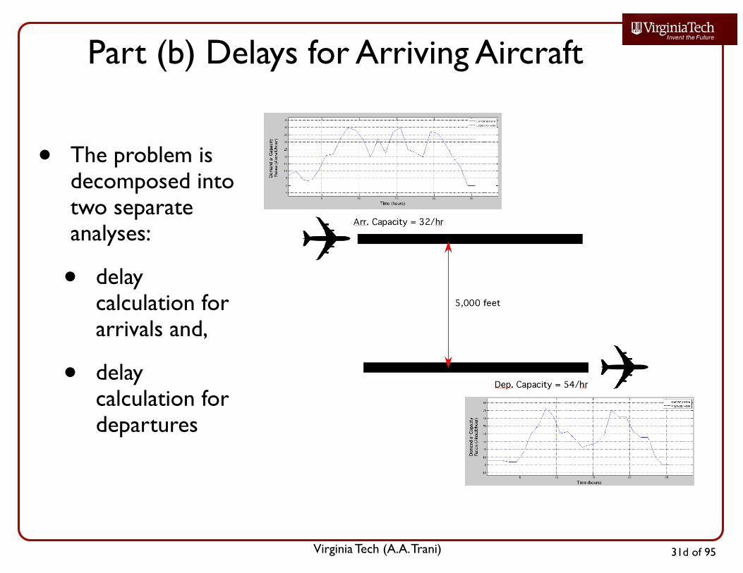
Example: Aircraft Delays Using Deterministic Queueing Model
• An airport has two parallel runways separated 5,000 feet away and oriented East-West
• The saturation capacity analysis for one of the runways yields the Pareto diagram shown in the following figure
• Assume that the fleet mix operating at both runways is the same
• The diagram assumes that the runway is operated in mixed mode
• The analysis was done for IFR conditions
29 of 95

Virginia Tech (A.A. Trani)
Airport Diagram
• Note: runways are used in segregated mode
29a of 95

Virginia Tech (A.A. Trani)
Pareto Diagram for a Single Runway at the Airport (Mixed Mode)
One-runway Pareto Diagram. Mixed Runway Use. IFR Conditions. Numbers in the Plot Represent (Departure, Arrival) Pairs.
30 of 95

Virginia Tech (A.A. Trani)
Airport Demand Function (Daily Demand)
Time (hrs)(Center of hourly interval)
Arrival demand(aircraft/hr)
Departure demand(aircraft/hr)
0.5 7 6
1.5 10 6
2.5 4 6
3.5 3 4
4.5 10 4
5.5 21 17
6.5 22 41
7.5 33 51
8.5 40 73
9.5 38 63
10.5 32 41
11.5 20 43
31 of 95

Virginia Tech (A.A. Trani)
Airport Demand Function (Daily Demand) - Part 2
Time (hrs)(Center of hourly interval)
Arrival demand(aircraft/hr)
Departure demand(aircraft/hr)
12.5 32 34
13.5 23 23
14.5 37 26
15.5 40 29
16.5 25 38
17.5 23 71
18.5 20 62
19.5 37 62
20.5 36 43
21.5 29 36
22.5 20 36
23.5 13 11
31a of 95

Virginia Tech (A.A. Trani)
Relevant Questions
a) Draw the Pareto capacity diagram for the complete airport runway system (i.e., both runways) if the runways are used in segregated mode in IFR conditions.
b) If the airport is operated in segregated mode, determine the average delay to arriving aircraft if the arrival demand function proposed by the airlines is shown in Table 1. Assume IFR conditions prevail in the design day.
c) If the airport is operated in segregated mode, determine the average delay to departing aircraft if the departure demand function proposed by the airlines is shown in Table 1. Assume IFR conditions prevail in the design day.
31b of 95
Virginia Tech (A.A. Trani)
Part (a) Pareto Diagram for Complete Airport (Segregated Mode)
31c of 95
Virginia Tech (A.A. Trani)
Part (b) Delays for Arriving Aircraft
• The problem is decomposed into two separate analyses:
• delay calculation for arrivals and,
• delay calculation for departures
31d of 95

Virginia Tech (A.A. Trani)
Part (b) Delays for Arriving Aircraft
• Arrival demand and arrival runway capacity
Periods where demand > capacity
31e of 95

Virginia Tech (A.A. Trani)
Part (b) Queue Length Function• Numerical integration solution for queue length function (Lt)
31f of 95
Use deterministic queue Matlab code: det_queue_enhanced.m
(see Matlab files for CEE 5614)
The maximum arrival queue length is estimated to be 14.53
aircraft at 10:30 AM in the design day

Virginia Tech (A.A. Trani)
Part (b) Integral of Queue Length Function
• Numerical integration solution for the area under the curve of the queue length function (Lt)
31g of 95
Use deterministic queue Matlab code: det_queue_enhanced.m
(see Matlab files for CEE 5614)
Total delay is estimated to be 70.84 aircraft-hours

Virginia Tech (A.A. Trani)
Part (b) Find the Average Arrival Delay
• Three queues were observed in the period of analysis (one day)
• Total number of aircraft delayed are calculated for the periods when the queues persist
31h of 95
Total delay is estimated to be 70.84 aircraft-hours
Period 1 Period 2 Period 3

Virginia Tech (A.A. Trani)
Part (b) Cumulative Arrivals Function
31i of 95

Virginia Tech (A.A. Trani)
Part (b) Cumulative Arrivals
31j of 95
Time (hrs) Cumulative Arrivals Arrivals in Queueing Period
7.4 87
274-87 = 187
13.25 274
274-87 = 187
14.15 298
405-298=107
17.5 405
405-298=107
19.2 445
546-445=101
22.34 546
546-445=101
Total Arrivals Queued 395

Virginia Tech (A.A. Trani)
• Total delay = 70.84 aircraft-hours
• Total aircraft delayed = 395 aircraft
• Average delay per aircraft = 0.179 hours (or 10.7 minutes)
Part (b) Find the Average Arrival Delay
31k of 95

Virginia Tech (A.A. Trani)
Part (c) Departure Delays
• Repeat the same process for departures
• Use departure saturation capacity found in the initial analysis (54 operations per hour)
31l of 95

Virginia Tech (A.A. Trani)
Part (c) Departure Demand Function
• Departure demand and departure runway capacity
Periods where departure demand > dep. capacity
31m of 95

Virginia Tech (A.A. Trani)
Part (c) Departure Queue Length Function
• Numerical integration solution for queue length function (Lt)
31o of 95
Use deterministic queue Matlab code: det_queue_enhanced.m
(see Matlab files for CEE 5614)
The maximum departure queue length is estimated to be 26.3 aircraft at 19:45 in
the design day

Virginia Tech (A.A. Trani)
Part (c) Integral of Departure Queue Length Function
• Numerical integration solution for the area under the curve of the queue length function (Lt)
31p of 95
Use deterministic queue Matlab code: det_queue_enhanced.m
(see Matlab files for CEE 5614)
Total delay is estimated to be 136.7 aircraft-hours

Virginia Tech (A.A. Trani)
Part (c) Cumulative Departures Function
31q of 95

Virginia Tech (A.A. Trani)
Part (c) Cumulative Departures
31r of 95
Time (hrs) Cumulative Departures Departures in Queueing Period
7.7 113
354-113 = 241
12.1 354
354-113 = 241
17 506
776-506=270
22 776
776-506=270
Total Departures Queued 511

Virginia Tech (A.A. Trani)
• Total delay = 135.7 aircraft-hours
• Total aircraft delayed = 511 aircraft
• Average delay per aircraft = 0.27 hours (or 16 minutes)
Part (b) Find the Average Arrival Delay
31s of 95

Virginia Tech (A.A. Trani)
Cumulative Demand and Supply Diagrams(for Departure Operations)
31t of 95

Virginia Polytechnic Institute and State University 32 of 95
Matlab Source Code for Deterministic Queueing Model (main file)
% Deterministic queueing simulation% T. Trani (Rev. Mar 99)global demand capacity time
% Enter demand function as an array of values over time
% general demand - capacity relationships%% demand = [70 40 50 60 20 10];% capacity = [50 50 30 50 40 50];% time = [0 10 20 30 40 50];
demand = [1500 1000 1200 500 500 500];capacity = [1200 1200 1000 1000 1200 1200];time = [0.00 1.00 1.500 1.75 2.00 3.00];

Virginia Polytechnic Institute and State University 33 of 95
% Compute min and maximum values for proper scaling in plotsmintime = min(time);maxtime = max(time);maxd = max(demand);maxc = max(capacity);mind = min(demand);minc = min(capacity);scale = round(.2 *(maxc+maxd)/2)minplot = min(minc,mind) - scale;maxplot = max(maxc,maxd) + scale;
po = [0 0]; % intial number of passengersto = mintime;tf = maxtime;tspan = [to tf];
% where:

Virginia Polytechnic Institute and State University 34 of 95
% to is the initial time to solve this equation% tf is the final time% tspan is the time span to solve the simulation
[t,p] = ode23('fqueue_2',tspan,po);
% Compute statistics
Ltmax = max(p(:,1));tdelay = max(p(:,2));a_demand = mean(demand);a_capacity = mean(capacity);
clc disp([blanks(5),'Deterministic Queueing Model ']) disp(' ') disp(' ') disp([blanks(5),' Average arrival rate (entities/time) = ', num2str(a_demand)])

Virginia Polytechnic Institute and State University 35 of 95
disp([blanks(5),' Average capacity (entities/time) = ', num2str(a_capacity)]) disp([blanks(5),' Simulation Period (time units) = ', num2str(maxtime)])
disp(' ') disp(' ') disp([blanks(5),' Total delay (entities-time) = ', num2str(tdelay)]) disp([blanks(5),' Max queue length (entities) = ', num2str(Ltmax)]) disp(' ')
pause
% Plot the demand and supply functions
plot(time,demand,'b',time,capacity,'k')xlabel('Time (minutes)')ylabel('Demand or Cpacity (Entities/time)')axis([mintime maxtime minplot maxplot])
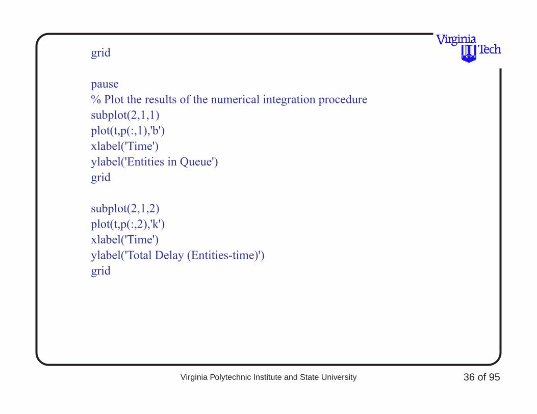
Virginia Polytechnic Institute and State University 36 of 95
grid
pause% Plot the results of the numerical integration proceduresubplot(2,1,1)plot(t,p(:,1),'b')xlabel('Time')ylabel('Entities in Queue')grid
subplot(2,1,2)plot(t,p(:,2),'k')xlabel('Time')ylabel('Total Delay (Entities-time)')grid

Virginia Polytechnic Institute and State University 37 of 95
Matlab Source Code for Deterministic Queueing Model (function file)
% Function file to integrate numerically a differential equation % describing a deterministic queueing system
function pprime = fqueue_2(t,p)global demand capacity time
% Define the rate equationsdemand_table = interp1(time,demand,t);capacity_table = interp1(time,capacity,t);
if (demand_table < capacity_table) & (p > 0) pprime(1) = demand_table - capacity_table; % rate of change in state variableelseif demand_table > capacity_table pprime(1) = demand_table - capacity_table; % rate of change in state variable

Virginia Polytechnic Institute and State University 38 of 95
else pprime(1) = 0.0; % avoids accumulation of entitiesend
pprime(2) = p(1); % integrates the delay curve over timepprime = pprime';

Virginia Polytechnic Institute and State University 39 of 95
Output of Deterministic Queueing Model
Deterministic Queueing Model Average arrival rate (entities/time) = 866.6667 Average capacity (entities/time) = 1133.3333 Simulation Period (time units) = 3 Total delay (entities-time) = 94.8925 Max queue length (entities) = 89.6247

Virginia Polytechnic Institute and State University 40 of 95
Stochastic Queueing Theory (Nomenclature per Hillier and Lieberman)
These models can only be generalized for simple arrival and departure functions since the involvement of complex functions make their analytic solution almost impossible to achieve. The process to be described first is the so-called birth and death process that is completely analogous to the arrival and departure of an entity from the queueing system in hand.
Before we try to describe the mathematical equations it is necessary to understand the basic principles of the stochastic queue and its nomenclature.
Virginia Polytechnic Institute and State University 41 of 95
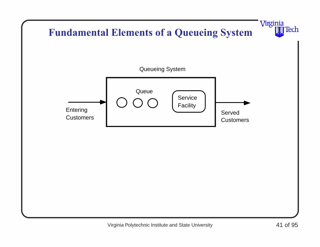
Fundamental Elements of a Queueing System
QueueServiceFacility
Queueing System
EnteringCustomers
ServedCustomers
Virginia Polytechnic Institute and State University 42 of 95
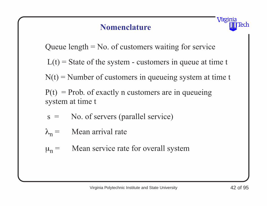
Nomenclature
Queue length = No. of customers waiting for service
L(t) = State of the system - customers in queue at time t
N(t) = Number of customers in queueing system at time t
P(t) = Prob. of exactly n customers are in queueing system at time t
s = No. of servers (parallel service)
λn = Mean arrival rate
µn = Mean service rate for overall system

Virginia Polytechnic Institute and State University 43 of 95
Other Definitions in Queueing Systems
If λn is constant for all n then (1/λ) it represents the interarrival time. Also, is µn is constant for all n > 1 (constant for each busy server) then µn = m service rate and (1/µ) is the service time (mean).
Finally, for a multiserver system sµ is the total service rate and also ρ = l/sµ is the utilization factor. This is the amount of time that the service facility is being used.

Virginia Polytechnic Institute and State University 44 of 95
Stochastic Queueing Systems
The idea behind the queueing process is to analyze steady-state conditions. Lets define some notation applicable for steady-state conditions,
N = No. of customers in queueing system
Pn = Prob. of exactly n customers are in queueing system
L = Expected no. of customers in queueing system
Lq = Queue length (expected)
W = Waiting time in system (includes service time)
Wq = Waiting time in queue
Virginia Polytechnic Institute and State University 45 of 95
There are some basic relationships that have beed derived in standard textbooks in operations research [Hillier and Lieberman, 1991]. Some of these more basic relationships are:
L = λW
Lq = λWq
The analysis of stochastic queueing systems can be easily understood with the use of “Birth-Death” rate diagrams as illustrated in the next figure. Here the transitions of a system are illustrated by the state conditions 0, 1, 2, 3,.. etc. Each state corresponds to a situation where there are n customers in the system. This implies that state 0 means that the system is idle (i,e., no customers), system at state 1 means there is one customer and so forth.

Virginia Polytechnic Institute and State University 46 of 95
Rate Diagram for Birth-and-Rate Process
Note: Only possible transitions in the state of the system are shown.
0 1 2 n-1
λλλλ0000 λλλλ1111
µµµµ1111 µµµµ2222
n
λλλλn-1
µµµµn
.... .... .... .... .... .... ....

Virginia Polytechnic Institute and State University 47 of 95
Stochastic Queueing Systems
For a queue to achieve steady-state we require that all rates in equal the rates out or in other words that all transitions out are equal to all the transitions in. This implies that there has to be a balance between entering and leaving entities.
Consider state 0. This state can only be reached from state 1 if one departure occurs. The steady state probability of being in state 1 (P1) represents the portion of the time that it would be possible to enter state 0. The mean rate at which this happens is µ1P1. Using the same argument the mean occurrence rate of the leaving incidents must be λ0 P0 to the balance equation,

Virginia Polytechnic Institute and State University 48 of 95
Stochastic Queueing Systems
µ1P1 = λ0P0
For every other state there are two possible transitions. Both into and out of the state.
λ0 P0 = P1µ1
λ0 P0 + µ2 P2 = λ1P1 + µ1 P1
λ1 P1 + µ3 P3 = λ2P2 + µ2 P2
λ2 P2 + µ4 P4 = λ3P3 + µ3 P3
until, λn-1 Pn-1 + µn+1 Pn+1 = λnµn + µn Pn

Virginia Polytechnic Institute and State University 49 of 95
Stochastic Queueing Systems
Since we are interested in the probabilities of the system in every state n want to know the Pn's in the process. The idea is to solve these equations in terms of one variable (say P0) as there is one more variable than equations.
For every state we have,
P1 = λ0 /µ1 P0
P2 = λlλ0 / µ1 µ2 P0
P3 = λ2 λ1 λ0 / µ1 µ2 µ3 P0
Pn+1 = λn ..... λ1 λ0 / µ1 µ2 ...... µn+1 P0

Virginia Polytechnic Institute and State University 50 of 95
Stochastic Queueing Systems
Let Cn be defined as,
Cn = λn-1 ..... λ1λ0 / µ1 µ2 ...... µn
Once this is accomplished we can determine the values of all probabilities since the sum of all have to equate to unity.
Pn
i 0=
n
∑ 1=
P0 Pn
i 1=
n
∑+ 1=

Virginia Polytechnic Institute and State University 51 of 95
Stochastic Queueing Systems
Solving for P0 we have,
Now we are in the position to solve for the remaining queue parameters, L the average no. of entities in the system, Lq, the average number of customers in the
P0 CnP0
i 1=
n
∑+ 1=
P01
1 Cn
i 1=
n
∑+
------------------------=

Virginia Polytechnic Institute and State University 52 of 95
queue, W, the average waiting time in the system and Wq the average waiting time in the queue.
Pn CnP0=
L nPn
n 1=
∞
∑=
Lq n s–( )Pn
n s=
∞
∑=
W Lλ---=
WqLq
λ-----=

Virginia Polytechnic Institute and State University 53 of 95
This process can then be repeated for specific queueing scenarios where the number of customers is finite, infinite, etc. and for one or multiple servers. All systems can be derived using “birth-death” rate diagrams.
Virginia Polytechnic Institute and State University 54 of 95
Stochastic Queueing Systems
Depending on the simplifying assumptions made, queueing systems can be solved analytically.
The following section presents equations for the following queueing systems when poisson arrivals and negative exponential service times apply:
a) Single server - infinite source (constant and )
b) Multiple server - infinite source (constant and )
c) Single server - finite source (constant and )
d) Multiple server - finite source (constant and )
λ µ
λ µ
λ µ
λ µ

Virginia Polytechnic Institute and State University 55 of 95
Stochastic Queueing Systems Nomenclature
The idea behind the queueing process is to analyze steady-state conditions. Lets define some notation applicable for steady-state conditions,
N = No. of customers in queueing system
Pn = Prob. of exactly n customers are in queueing system
L = Expected no. of customers in queueing system
Lq = Queue length (expected)
W = Waiting time in system (includes service time)
Wq = Waiting time in queue

Virginia Polytechnic Institute and State University 56 of 95
Stochastic Queueing Systems
There are some basic relationships that have beed derived in standard textbooks in operations research [Hillier and Lieberman, 1991]. Some of these more basic relationships are:
L = λW
Lq = λWq

Virginia Polytechnic Institute and State University 57 of 95
Stochastic Queueing Systems
Single server - infinite source (constant and )
Assumptions:
a) Probability between arrivals is negative exponential with parameter
b) Probability between service completions is negative exponential with parameter
c) Only one arrival or service occurs at a given time
λ µ
λn
µn

Virginia Polytechnic Institute and State University 58 of 95
Single server - Infinite Source (Constant and )
Utilization factor
for n = 0,1,2,3,.....
expected number of entities in the system
expected no. of entities in the queue
λ µ
ρ λ µ⁄=
P01
1 ρn
n 1=
∞
∑+
----------------------- ρn
n 0=
∞
∑
1–
11 ρ–------------
1–
1 ρ–= = = =
Pn ρnP0 1 ρ–( )ρn= =
L λµ λ–------------=
Lqλ2
µ λ–( )µ---------------------=

Virginia Polytechnic Institute and State University 59 of 95
average waiting time in the queueing
system
average waiting time in the queue
probability distribution of waiting times
(including the service potion in the SF)
W 1µ λ–------------=
Wqλ
µ λ–( )µ---------------------=
P W t>( ) e µ 1 ρ–( )t–=

Virginia Polytechnic Institute and State University 60 of 95
Multiple Server
Infinite source (constant and )
Assumptions:
a) Probability between arrivals is negative exponential with parameter
b) Probability between service completions is negative exponential with parameter
c) Only one arrival or service occurs at a given time
λ µ
λn
µn

Virginia Polytechnic Institute and State University 61 of 95
Multiple Server - Infinite Source (constant , )
utilization factor of the facility
idle probability
probability of n entities in the system
λ µ
ρ λ sµ⁄=
P0 1 λ µ⁄( )n
n!----------------- λ µ⁄( )s
s!----------------- 1
1 λ sµ⁄( )–--------------------------- +
n 0=
s 1–
∑ ⁄=
Pn
λ µ⁄( )n
n!-----------------P0
λ µ⁄( )n
s!sn s–-----------------P0
=
0 n s≤ ≤
n s≥

Virginia Polytechnic Institute and State University 62 of 95
expected number of entities in system
expected number of entities in queue
average waiting time in queue
average waiting time in system
Finally the probability distribution of waiting times is,
LρP0
λµ---
s
s! 1 ρ–( )2----------------------- λ
µ---+=
Lq
ρP0λµ---
s
s! 1 ρ–( )2-----------------------=
WqLq
λ-----=
W Lλ--- Wq
1λ---+= =

Virginia Polytechnic Institute and State University 63 of 95
if then use
P W t>( ) e µt– 1P0
λµ---
s
s! 1 ρ–( )--------------------- 1 e µt s 1– λ µ⁄–( )––
s 1– λ µ⁄–-------------------------------- +=
s 1– λ µ⁄– 0=
1 e µt s 1– λ µ⁄–( )––s 1– λ µ⁄–
-------------------------------- µt=

Virginia Polytechnic Institute and State University 64 of 95
Single Server - Finite Source (constant and )
Assumptions:
a) Interarrival times have a negative exponential PDF with parameter
b) Probability between service completions is negative exponential with parameter
c) Only one arrival or service occurs at a given time
d) M is the total number of entities to be served (calling population)
λ µ
λn
µn

Virginia Polytechnic Institute and State University 65 of 95
Single Server - Finite Source (constant and )
utilization factor of the facility
idle probability
for probability
of n entities in the system
expected number of entities in
queue
λ µ
ρ λ µ⁄=
P0 1 M!M n–( )!
-------------------- λ µ⁄( )n
n 0=
M
∑⁄=
PnM!
M n–( )!-------------------- λ µ⁄( )nP0= n 1 2 3 …M, , ,=
Lq M µ λ+λ
------------- 1 P0–( )–=

Virginia Polytechnic Institute and State University 66 of 95
expected number of entities in
system
average waiting time in queue
average waiting time in system
where:
average arrival rate
L M µλ--- 1 P0–( )–=
WqLq
λ-----=
W L
λ---=
λ λ M L–( )=
Virginia Polytechnic Institute and State University 67 of 95
Multiple Server Cases
Finite source (constant and )
Assumptions:
a) Interarrival times have a negative exponential PDF with parameter
b) Probability between service completions is negative exponential with parameter
c) Only one arrival or service occurs at a given time
d) M is the total number of entities to be served (calling population)
λ µ
λn
µn

Virginia Polytechnic Institute and State University 68 of 95
Multiple Server - Finite Source (constant and )
utilization factor of the facility
idle probability
if
λ
µ
ρ λ µ⁄ s=
P0 1 M!M n–( )!n!
-------------------------- λ µ⁄( )n
M!
M n–( )!s!sn s–---------------------------------- λ µ⁄( )n
n s=
M
∑+n 0=
s 1–
∑⁄=
Pn
M!M n–( )!n!
-------------------------- λ µ⁄( )nP0
M!M n–( )!s!sn s–
---------------------------------- λ µ⁄( )nP0
0
=
0 n s≤ ≤
s n M≤ ≤
n M≥

Virginia Polytechnic Institute and State University 69 of 95
expected number of entities in
queue
expected number of entities in system
average waiting time in queue
average waiting time in system
Lq n s–( )Pn
n s=
M
∑=
L nPn
n 0=
M
∑ nPn Lq s 1 Pn
n 0=
s 1–
∑–
+ +n 0=
s 1–
∑= =
WqLq
λ-----=
W L
λ---=

Virginia Polytechnic Institute and State University 70 of 95
where:
average arrival rateλ λ M L–( )=

Virginia Polytechnic Institute and State University 71 of 95
Example (3): Level of Service at Security Checkpoints
The airport shown in the next figures has two security checkpoints for all passengers boarding aircraft. Each security check point has two x-ray machines. A survey reveals that on the average a passenger takes 45 seconds to go through the system (negative exponential distribution service time).
The arrival rate is known to be random (this equates to a Poisson distribution) with a mean arrival rate of one passenger every 25 seconds.
In the design year (2010) the demand for services is expected to grow by 60% compared to that today.
Virginia Polytechnic Institute and State University 72 of 95
Relevent Operational Questions
a) What is the current utilization of the queueing system (i.e., two x-ray machines)?
b) What should be the number of x-ray machines for the design year of this terminal (year 2020) if the maximum tolerable waiting time in the queue is 2 minutes?
c) What is the expected number of passengers at the checkpoint area on a typical day in the design year (year 2020)? Assume a 60% growth in demand.
d) What is the new utilization of the future facility?
e) What is the probability that more than 4 passengers wait for service in the design year?

Virginia Polytechnic Institute and State University 73 of 95
Airport Terminal Layout

Virginia Polytechnic Institute and State University 74 of 95
Security Check Point Layout
Queueing System Service Facility

Virginia Polytechnic Institute and State University 75 of 95
Security Check Point Solutions
a) Utilization of the facility, ρ. Note that this is a multiple server case with infinite source.
ρ = λ / (sµ) = 144/(2*80) = 0.90
Other queueing parameters are found using the steady-state equations for a multi-server queueing system with infinite population are: Idle probability = 0.052632 Expected No. of customers in queue (Lq) = 7.6737 Expected No. of customers in system (L) = 9.4737 Average Waiting Time in Queue = 192 s Average Waiting Time in System = 237 s

Virginia Polytechnic Institute and State University 76 of 95
b) The solution to this part is done by trail and error (unless you have access to design charts used in queueing models. As a first trial lets assume that the number of x-ray machines is 3 (s=3).
Finding Po,
Po = .0097 or less than 1% of the time the facility is idle
Find the waiting time in the queue,
Wq = 332 s
Since this waiting time violates the desired two minute maximum it is suggested that we try a higher number of x-ray machines to expedite service (at the expense of
P0λ µ⁄( )2
n!----------------- λ µ⁄( )s
s!----------------- 1
1 λ sµ⁄( )–--------------------------- +
n 0=
s 1–
∑=

Virginia Polytechnic Institute and State University 77 of 95
cost). The following figure illustrates the sensitivity of Po and Lq as the number of servers is increased.
Note that four x-ray machines are needed to provide the desired average waiting time, Wq.

Virginia Polytechnic Institute and State University 78 of 95
Sensitivity of Po with S
Note the quick variations in Po as S increases.
3 4 5 6 7 80
0.01
0.02
0.03
0.04
0.05
0.06
S - No. of Servers
Po
- Id
le P
roba
bilit
y
TextEnd

Virginia Polytechnic Institute and State University 79 of 95
Sensitivity of L with S
3 4 5 6 7 80
5
10
15
20
25
S - No. of Servers
L -
Cus
tom
ers
in S
yste
m
TextEnd

Virginia Polytechnic Institute and State University 80 of 95
Sensitivity of Lq with S
3 4 5 6 7 80
5
10
15
20
25
S - No. of Servers
Lq -
Cus
tom
ers
in Q
ueue
TextEnd

Virginia Polytechnic Institute and State University 81 of 95
Sensitivity of Wq with S
This analysis demonstrates that 4 x-ray machines are needed to satisfy the 2-minute operational design constraint.
3 4 5 6 7 80
0.02
0.04
0.06
0.08
0.1
0.12
S - No. of Servers
Wq
- W
aitin
g T
ime
in th
e Q
ueue
(hr
)
TextEnd
Waiting time constraint

Virginia Polytechnic Institute and State University 82 of 95
Sensitivity of W with S
Note how fast the waiting time function decreases with S
3 4 5 6 7 80
0.01
0.02
0.03
0.04
0.05
0.06
0.07
0.08
0.09
0.1
S - No. of Servers
W -
Tim
e in
the
Sys
tem
(hr
)
TextEnd

Virginia Polytechnic Institute and State University 83 of 95
Security Check Point Results
c) The expected number of passengers in the system is (with S = 4),
L = 4.04 passengers in the system on the average design year day.
d) The utilization of the improved facility (i.e., four x-ray machines) is
ρ = λ / (sµ) = 230/ (4*80) = 0.72
LρP0
λµ---
s
s! 1 ρ–( )2----------------------- λ
µ---+=

Virginia Polytechnic Institute and State University 84 of 95
e) The probability that more than four passengers wait for service is just the probability that more than eight passengers are in the queueing system, since four are being served and more than four wait.
where,
if
if
P n 8>( ) 1 Pn
n 0=
8
∑–=
Pnλ µ⁄( )n
n!-----------------P0= n s≤
Pnλ µ⁄( )n
s!sn s–-----------------P0= n s>

Virginia Polytechnic Institute and State University 85 of 95
from where, Pn > 8 is 0.0879.
Note that this probability is low and therefore the facility seems properly designed to handle the majority of the expected traffic within the two-minute waiting time constraint.

Virginia Polytechnic Institute and State University 86 of 95
PDF of Customers in System (L)
The PDF below illustrates the stochastic process resulting from poisson arrivals and neg. exponential service times
0 2 4 6 8 10 12 14 16 18 200
0.02
0.04
0.06
0.08
0.1
0.12
0.14
0.16
0.18
0.2
Number of entities
Pro
babi
lity
TextEnd

Virginia Polytechnic Institute and State University 87 of 95
Matlab Computer Code
% Multi-server queue equations with infinite population
% Sc = Number of servers% Lambda = arrival rate% Mu = Service rate per server% Rho = utilization factor% Po = Idle probability% L = Expected no of entities in the system% Lq = Expected no of entities in the queue% nlast - last probability to be computed
% Initial conditions
S=5; Lambda=3; Mu = 4/3;

Virginia Polytechnic Institute and State University 88 of 95
nlast = 10; % last probability value computed Rho=Lambda/(S*Mu);
% Find Po Po_inverse=0; sum_den=0;
for i=0:S-1 % for the first term in the denominator (den_1) den_1=(Lambda/Mu)^i/fct(i); sum_den=sum_den+den_1; end
den_2=(Lambda/Mu)^S/(fct(S)*(1-Rho)); % for the second part of den (den_2) Po_inverse=sum_den+den_2; Po=1/Po_inverse

Virginia Polytechnic Institute and State University 89 of 95
% Find probabilities (Pn)
Pn(1) = Po; % Initializes the first element of Pn column vector to be Pon(1) = 0; % Vector to keep track of number of entities in system
% loop to compute probabilities of n entities in the system
for j=1:1:nlast n(j+1) = j; if (j) <= S Pn(j+1) = (Lambda/Mu)^j/fct(j) * Po; else Pn(j+1) = (Lambda/Mu)^j/(fct(S) * Sc^(j-S)) * Po; endend
% Queue measures of effectiveness
Lq=(Lambda/Mu)^S*Rho*Po/(fct(S)*(1-Rho)^2)

Virginia Polytechnic Institute and State University 90 of 95
L=Lq+Lambda/Mu Wq=Lq/Lambda W = L/Lambda plot(n,Pn) xlabel('Number of entities') ylabel('probability')

Virginia Polytechnic Institute and State University 91 of 95
Example 4 - Airport Operations
Assume IFR conditions to a large hub airport with
• Arrival rates to metering point are 45 aircraft/hr
• Service times dictated by in-trail separations (120 s headways)
Runway 09L-27R
Runway 09R-27L
4300 ft.
Common ArrivalMetering Point

Virginia Polytechnic Institute and State University 92 of 95
Some Results of this Simple Model
Parameter Numerical Values
45 aircraft/hr to arrival metering point
30 aircraft per runway per hour
0.143 0.750
3.42 aircraft (includes those in service)
2.57 minutes per aircraft
4.57 minutes per aircraft
λ
µ
Po
ρ
L
Wq
W

Virginia Polytechnic Institute and State University 93 of 95
Sensitivity Analysis
Lets vary the arrival rate ( ) from 20 to 55 per hour and see the effect on the aircraft delay function.
λ
20 25 30 35 40 45 50 550
2
4
6
8
10
12
Arrival Rate (Aircraft/hr)
Wai
ting
Tim
e (m
in)
Virginia Polytechnic Institute and State University 94 of 95
Sensitivity of with Demand
The following diagram plots the sensitivity of the expected number of aircraft holding vs. the demand function
Lq
20 25 30 35 40 45 50 550
2
4
6
8
10
Arrival Rate (Aircraft/hr)
Hol
ding
Airc
raft

Virginia Tech (A.A. Trani)
Example # 5 Seaport Operations
• Seaport facility with 4 berths (a beth is an area where ships dock for loading/unloading)
• Arrivals are random with a mean of 2.5 arrivals per day
• Average service time for a ship is 0.9 days (assume a negative exponential distribution)
• Find:
• Expected waiting time and total cost of delays per year if the average delay cost is $12,000 per day per ship
94a

Virginia Tech (A.A. Trani)
Solution (use Stochastic Queueing Model - Infinite Population)
94b

Virginia Tech (A.A. Trani)
Solution (Seaport Example)
94c

Virginia Tech (A.A. Trani)
Solution (Seaport Example)
94d

Virginia Tech (A.A. Trani)
Others Uses of Queueing Models(Facilities Planning)
• Queueing models can be used to estimate the life cycle cost of a facility
• Using the expected delays we can estimate times when a facility needs to be upgraded
• For example,
• Suppose the demand function (i.e., number of ships arriving to port) for ships arriving to port increases 10% per year
• Determine the year when new berths will be required if the port authority wants to maintain waiting times below 0.5 days.
94e

Virginia Tech (A.A. Trani)
Calculations for Seaport Example
Time (years)0 1 2 3
94f

Virginia Tech (A.A. Trani)
Calculations for Seaport Example
94g
Virginia Tech (A.A. Trani)
Calculations for Seaport Example
94h

Virginia Tech (A.A. Trani)
Undiscounted Annual Delay Costs(Lag Solution)
$12,000 per hour per shipdelay costs
94i

Virginia Tech (A.A. Trani)
Construction Cost Profile (Seaport)(Lag Solution)
$50 Million per Berth
94j

Virginia Tech (A.A. Trani)
Total Annual Cost (Seaport - Lag Solution)
$50 Million per Berth
94k

Virginia Tech (A.A. Trani)
Lead Solution for Berth Construction
94l

Virginia Tech (A.A. Trani)
Lead Solution for Berth Construction
94m

Virginia Tech (A.A. Trani)
Comparing Both SolutionsLife Cycle Cost Analysis
94n

Virginia Polytechnic Institute and State University 95 of 95
Conclusions About Analytic Queueing Models
Advantages:• Good traceability of causality between variables
• Good only for first order approximations
• Easy to implement
Disadvantages:• Too simple to analyze small changes in a complex system
• Cannot model transient behaviors very well
• Large errors are possible because secondary effects are neglected
• Limited to cases where PDF has a close form solution