, 20120653, published 27 February 2013469 2013 Proc. R. Soc. A Gareth Wyn Jones and L. Mahadevan quasi-conformal mappingsPlanar morphometry, shear and optimal  

References3.full.html#ref-list-1http://rspa.royalsocietypublishing.org/content/469/2153/2012065

This article cites 31 articles, 2 of which can be accessed free

Subject collections

(77 articles)differential equations   � (47 articles)computational mathematics   �

(261 articles)applied mathematics   � Articles on similar topics can be found in the following collections

Email alerting service herethe box at the top right-hand corner of the article or click Receive free email alerts when new articles cite this article - sign up in

http://rspa.royalsocietypublishing.org/subscriptions go to: Proc. R. Soc. ATo subscribe to

on March 1, 2013rspa.royalsocietypublishing.orgDownloaded from

rspa.royDownloaded from

rspa.royalsocietypublishing.org

ResearchCite this article: Jones GW, Mahadevan L.2013 Planar morphometry, shear and optimalquasi-conformal mappings. Proc R Soc A 469:20120653.http://dx.doi.org/10.1098/rspa.2012.0653

Received: 1 November 2012Accepted: 24 January 2013

Subject Areas:applied mathematics, computationalmathematics, differential equations

Keywords:quasi-conformal mapping, shear,optimization, morphometry

Author for correspondence:L. Mahadevane-mail: lm@seas.harvard.edu

Planar morphometry, shearand optimal quasi-conformalmappingsGareth Wyn Jones and L. Mahadevan

Department of Physics, School of Engineering and Applied Sciences,Wyss Institute for Biologically Inspired Engineering, HarvardUniversity, 29 Oxford Street, Cambridge, MA 02138, USA

To characterize the diversity of planar shapes insuch instances as insect wings and plant leaves, wepresent a method for the generation of a smoothmorphometric mapping between two planar domainswhich matches a number of homologous points. Ourapproach tries to balance the competing requirementsof a descriptive theory which may not reflectmechanism and a multi-parameter predictive theorythat may not be well constrained by experimentaldata. Specifically, we focus on aspects of shape ascharacterized by local rotation and shear, quantifiedusing quasi-conformal maps that are defined preciselyin terms of these fields. To make our choice optimal,we impose the condition that the maps vary asslowly as possible across the domain, minimizingtheir integrated squared-gradient. We implement thisalgorithm numerically using a variational principlethat optimizes the coefficients of the quasi-conformalmap between the two regions and show results forthe recreation of a sample historical grid deformationmapping of D’Arcy Thompson. We also deployour method to compare a variety of Drosophilawing shapes and show that our approach allowsus to recover aspects of phylogeny as markedby morphology.

1. IntroductionRelative growth processes in living systems leadto changes in size and shape. Morphometry, themeasurement of shape, is often the first descriptive steptowards explaining the development and evolution ofform in animate and inanimate patterns. Morphometrics,the quantitative study of shape differences betweenhomologous objects, analyses this in terms of a mappingthat quantifies the relative positioning of specific

on March 1, 2013alsocietypublishing.org

c© 2013 The Author(s) Published by the Royal Society. All rights reserved.

2

rspa.royalsocietypublishing.orgProcRSocA469:20120653

..................................................

on March 1, 2013rspa.royalsocietypublishing.orgDownloaded from

(a)(b)

Figure 1. An example of D’Arcy Thompson’s theory of transformations implemented via a deformable grid. A Cartesian gridsuperimposed on (a) Scarus is deformed in such away that when superimposed on (b) Pomacanthus homologous points in eachfish have similar coordinates on the grid. Reproduced with permission from Thompson [1].

landmarks, point-like features in the shapes or on the boundaries of these structures. Theidentification of such a mapping between two homologous shapes has its roots in the seminalwork of D’Arcy Thompson [1], who characterized a ‘theory of transformations’ for a class ofplanar projections of biological shapes in terms of a grid drawn over a particular shape and thendeformed to approximately fit a second, as seen in the example shown in figure 1.

Thompson’s ambitions for his grid method were twofold. Firstly, he aimed to uncover thephysical basis behind the deformation. In his words [1], once the transformation is known, ‘itwill be a comparatively easy task . . . to postulate the direction and magnitude of the forcecapable of effecting the required transformation’. The second aim was to ensure that the griddeformation chosen was as elementary as possible while still matching homologous landmarksin the grid coordinates. Thompson further said that whatever process caused the deformation, ‘itis essential that our structure vary in its entirety, or at least that “independent variants” shouldbe relatively few’, citing Occam’s razor. Although Thompson provided no quantitative way ofcalculating the transformations [2], early qualitative approaches included studies of amphibianlarval development and ceratopsian dinosaur skulls [3–5]. Additionally, the images of deformedgrids are useful in pointing out where two homologous structures most differ, using ink-dotexperiments on growing leaves [6] or in simulations of neurulation [7] provided. Stimulatedby D’Arcy Thompson, Medawar [8] proposed that the creation of deformation grids could bestandardized by assuming that the x- and y-coordinates were transformed according to allometricscaling laws. However, this puts these axes in a privileged position; certainly for an arbitraryshape comparison it is impractical to assume that there will be one set of axes that remainsorthogonal under the mapping between them. Sneath [9] also developed a method to calculatea mapping based on the Cartesian grid, but in this case the coordinates of the destination gridwere polynomial functions of the source coordinates. The coefficients of the polynomials werecalculated to match landmarks under the mapping, and correspond to Thompson’s ‘independentvariants’. This appears to be the first method to compute mappings, but in essence it is a two-dimensional analogue to a polynomial curve-fitting exercise with coefficients that are hard torelate to local physical or biological quantities. One simple way of constructing a mappingbased on landmark data is to connect the points to form a triangular tessellation, and toassume that the mapping is affine in each triangle: this is the finite-element scaling method [10].A drawback of this mapping is that it is not unique, since there is no canonical way toselect the triangular tessellation.

Bookstein’s first studies [11] set out to calculate deformation mappings that ensured theproper correspondence between the boundaries of the two structures. His initial calculationsapproximated the shapes by simple polygons and calculated the correspondence using harmonicmaps, ignoring internal constraints. In a later study [12], he chose a mapping that minimizedthe ‘roughness’ of the deformation subject to internal point constraints (equivalent to demandingthat the components of the deformation satisfy biharmonic equations with a point force at eachinternal landmark). In both cases, the boundary correspondence was prescribed explicitly, byinterpolating landmark points on the boundary. Eventually, the idea of creating mappings thatwere restricted to the interior of the shapes was abandoned in favour of the thin plate spline

3

rspa.royalsocietypublishing.orgProcRSocA469:20120653

..................................................

on March 1, 2013rspa.royalsocietypublishing.orgDownloaded from

method [13], eliminating the distinction between boundary and interior landmarks, so that thesource and destination objects are defined solely by the positions of these landmark points. This isanalogous to the problem of finding the shape of a thin elastic plate, infinite in extent, constrainedto prescribed elevations at certain landmark points in the plane, and determined by the solutionof the biharmonic equation with a point force at each landmark point. To calculate the thin platespline mapping between the source and destination shapes, this equation is solved twice: for boththe x- and y-components of the deformation. Where landmark data on the boundary is sparse,one may discretize it and use semilandmarks, whose variation is constrained to be tangentialto the boundary. This method has become ubiquitous in the field of morphometry, especiallybecause its linearity has led to a fruitful synthesis with widely used statistical methods, such askriging [14,15].

A complementary approach borrows ideas from image registration in medical applicationssuch as MRI and CATscans which involves constructing the deformation that would bring oneimage in registration with another—precisely the original aim of Thompson. Such methods haveled to the field of pattern theory [16,17] and its relatives such as computational anatomy [18]and have become essential tools for analysing images of highly complex organs, primarilymotivated by brain imaging and the calculation of variations in brain shape and the physicalcharacterizations of certain brain pathologies.

These mappings inspired by Thompson’s original grid deformation have usually concentratedon only one of Thompson’s aims, namely the parsimony of the mapping, or at least that it shouldbe as simple as possible. The second aim, that the mapping should lead to insights into thephysical origin of the deformation, has been largely neglected, partly because of the assumptionthat shape change is directly linked solely to genetic variation. While this is certainly true at onelevel [19], it has also become increasingly clear that the genetic influence on morphogenesis ismediated by a combination of both developmental and physical processes [20–23]. Indeed, rathergenerally, there is increasing evidence in a variety of systems that during development, genesinfluence the distribution of biochemical gradients, or morphogenetic fields [24], which couldin turn change the rate of relative growth and rheology of a developing tissue. A growth fieldin linear elastic or viscoelastic materials, for instance, appears as a distributed body force in theequations of equilibrium, providing a possible interpretation for Thompson’s use of the word‘force’ in describing the physical basis of shape change, and this has become an area of increasingstudy recently [25,26].

Thus, an ideal for morphometry is to provide a framework within which descriptive mappingsthat characterize shape may be married to predictive models of the processes that underlie shapes.Of the methods described earlier, the closest to this philosophy are the physics-based imageregistration methods [27,28], containing distributed force fields as hypothesized by Thompson.For instance, in the method of Bajcsy et al. [27], the source image is treated as an elasticbody which is deformed by means of a distributed body force, chosen so that the resultclosely matches the destination image. Alternatively, Christensen et al. [28] treat the imagebeing deformed as a viscous fluid. Further examples are provided by Holden [29]. Modern-day implementations of such physics-based registration often take the form of Lagrangian-baseddeformation calculations [18], where the physics defines an energy satisfied by the (time-dependent) deformation. The deformation is found by solving the partial differential equation(PDE) arising from the minimization of this energy (subject to landmark preservation). However,the mappings here are over the whole image in question rather than restricted to the deformingobject itself, so the elastic or viscous properties of the deformation cannot be interpreted asbelonging to the object. We may then ask if it is possible to balance the two goals set out byD’Arcy Thompson, can we derive a simple mapping that allows us to efficiently compare shapeswhile also providing a modicum of insight into the underlying physical processes?

Here we present a method to compare two homologous shapes (Ω0 and Ω1); we will limitourselves to two dimensions in terms of a mapping from Ω0 to Ω1, with landmark points inΩ0 mapped to the corresponding points in Ω1 both for mathematical simplicity, and becausethere are many nice biological planforms where we can still deploy these methods fruitfully.

4

rspa.royalsocietypublishing.orgProcRSocA469:20120653

..................................................

on March 1, 2013rspa.royalsocietypublishing.orgDownloaded from

F FE EA

W0 W1

q

A

BB

G GD D

C Cy v

ux

Figure 2. A mapping between Ω0 and Ω1 can be described mathematically by a relationship between (u, v) and (x, y).Points A–G are to be kept fixed under the mapping. Inset: definition of the boundary parameter θ . (Online version in colour.)

As desiderata, we would like our mapping to allow us to identify not just points in Ω0 andthe corresponding points in Ω1, but also interpolate between the landmark points. Furthermore,given an infinitesimally small circle in Ω0, its image under the mapping should tell us about thenature of the mapping at that location: in general the image will be an ellipse, with its orientationcharacterizing the local rotation, its eccentricity measuring the local shear and the change inarea relative to the original circle describing the local expansion or contraction of the materialat that point. Since the space of dilatations and shears, combined with rotations completelydescribes the kinematics of growth and deformations, if our mapping reflects these measures,they may be naturally correlated with predictive models of the shape difference betweenΩ0 and Ω1.

Mathematically, our mapping between the domains Ω0 and Ω1 should allow us to fix anumber of points along the boundary and in the interior of the domain, as shown in figure 2,and are characterized in terms of the functions (u(x, y), v(x, y)) ∈ Ω1, with (x, y) ∈ Ω0. A predictivetheory of morphometrics would require some dynamical laws for these functions, reflecting theirmaterial properties, the biochemical gradients that drive growth or shrinkage, coupled with thebalance laws for mass and momentum conservation. The genetic or evolutionary influence onthe shape changes is manifested through parameters in these equations. It is in the determinationof these parameters that Thompson’s parsimony requirement should apply (in contrast to thepreviously cited models, which choose the deformation itself to be as simple as possible). Thus,given a biophysical model, we seek the simplest parameter field that can explain the shapechange observed.

It is natural that our mapping between Ω0 and Ω1 be a bijection, mapping the boundariesto each other and preserving the positions of homologous landmarks, with some freedomcharacterized by a dependence on an underlying parameter field, that encapsulates the influenceof evolutionary or genetic processes. In a complete description, these parameters and the mappingwould follow from genetics, biochemical and biophysical principles. In the more limited settingconsidered here, our mapping should reflect as much of these desiderata as possible, andour morphospaces should be described by parameter fields that are the simplest ones able tocharacterize the difference between the shapes.

Quasi-conformal mappings are relatively simple mappings that satisfy the properties above:they are not as rigid as conformal maps or thin plate splines in that they have free parameters,indeed they have an entire function that is unknown, and yet they are relatively simple tocompute numerically. The equations governing such mappings incorporate a parameter fieldwhich prescribes the orientation and eccentricity of local patches characterized in terms ofellipses, and thus reflect the natural physical processes associated with planar tissue shaping, butare not as complex as a complete description of the biophysics would entail in terms of materialrheology and relative growth rates as embedded in a continuum mechanical field theory. Given

5

rspa.royalsocietypublishing.orgProcRSocA469:20120653

..................................................

on March 1, 2013rspa.royalsocietypublishing.orgDownloaded from

the freedom associated with the infinite choices of the parameter field that can describe any givenshape change, we postulate our choice of one based on a simple criterion: choose one that variesspatially as little as possible, postulated as an optimization principle.

In §2, we set the stage by describing the basic properties of quasi-conformal maps that werequire. In §§3 and 4, we describe the construction of optimal quasi-conformal maps, while in §5,we discuss a numerical method for their determination and present a number of examples thatilluminate our theory, drawn from D’Arcy Thompson’s work as well as recent work on insect-wing shape.

2. A primer on quasi-conformal mapsWe start with a brief summary of some of the properties of quasi-conformal maps that we needfor our exposition; a complete introduction can be found in the monograph of Ahlfors [30]. Quasi-conformal maps were originally developed as a generalization of the well-known conformal mapsby relaxing the condition of conformality that does not allow for any shear deformations, and yetstill well suited to treatment by complex analysis. For a general mapping u = u(x, y), v = v(x, y)

between two planar regions, we may immediately write w = u + iv and z = x + iy, so that themapping can be represented by w = w(z, z) where z = x − iy. For infinitesimally small regions of(x, y) space, characterized by the differentials (dx, dy), the mapping becomes

du = uxdx + uy dy and dv = vx dx + vy dy, (2.1)

which is an affine map that takes infinitesimally small circles to infinitesimally small ellipses,with subscripts representing partial differentiation, i.e. ab = ∂a/∂b. Equivalently, we have dw =wz dz + wz dz, and so if an infinitesimal circle in Ω0 is represented as dz = dreiθ , then

dw = dr ei(α+β)/2[|wz| exp

(i(

θ − (β − α)

2

))+ |wz| exp

(−i(

θ − (β − α)

2

))], (2.2)

where wz = |wz|eiα and wz = |wz|eiβ . This equation represents an ellipse whose long axis is at anangle (α + β)/2 to the horizontal, and with a ratio of long axis to short axis given by

Dw = |wz| + |wz||wz| − |wz|

. (2.3)

We note that Dw = 1 if and only if wz = 0, which are just the Cauchy–Riemann equations forconformal maps wherein infinitesimally small circles are mapped to infinitesimally small circles.We may write Dw = (1 + |μ|)/(1 − |μ|), where the quantity μ = wz/wz is often misleadinglyknown as the complex dilatation or the first complex dilatation (misleading because in commonusage, ‘dilatation’ commonly refers to area changes, whereas μ only encodes the eccentricity andorientation of image ellipses), although we will persist with this usage. For later use, we also notethat the second complex dilatation is another important parameter, given by ν = wz/(wz), with|μ| = |ν|.

With these properties defined, a mapping w = w(z, z) is said to be quasi-conformal if Dw isbounded, and specifically it is called K-quasi-conformal if Dw ≤ K. It follows immediately that a1-quasi-conformal map is a conformal map. This condition on Dw naturally induces a conditionon |μ| (and on |ν|): we need |μ| = |ν| ≤ M < 1 for the map to be defined as quasi-conformal, whereM = (K − 1)/(K + 1). Two further properties of quasi-conformal maps that we will find useful are(i) they can be composed to produce further quasi-conformal mappings; thus the compositionof a K1-quasi-conformal and a K2-quasi-conformal mapping is K1K2-quasi-conformal, and (i) theinverse of a quasi-conformal map is also a quasi-conformal map.

From the definitions of μ and ν, we obtain the following differential equations for w:

∂w∂ z

= μ(z, z)∂w∂z

and∂w∂ z

= ν(z, z)(

∂w∂z

). (2.4)

6

rspa.royalsocietypublishing.orgProcRSocA469:20120653

..................................................

on March 1, 2013rspa.royalsocietypublishing.orgDownloaded from

known as the Beltrami equation and the conjugate Beltrami equation, respectively, whosesolutions (with the restriction on |μ| or |ν|) are quasi-conformal maps. We note that if μ = ν = 0,Dw = 1 and hence the mappings are conformal—and indeed in this limit both the Beltramiequations reduce to the Cauchy–Riemann equation ∂w/∂ z = 0.

While either of the equations in (2.4) can be solved to give a quasi-conformal map with thedesired shear properties, the conjugate Beltrami equation may be derived naturally from a simplevariational principle (presented in §4). This makes it amenable to solve (2.4)2, given ν and theboundary of the image (∂Ω1) using a Galerkin or finite-element method, and thus find a quasi-conformal map from Ω0 to Ω1. However, we must note the map will not be unique, as we canalways compose the computed map with a conformal map, which has three degrees of freedom,and the composite map will have the same distribution of ν. With this caveat, we may writeκ(x, y) = �(ν), λ(x, y) = �(ν), and thus the required quasi-conformal map solution as

u = u(x, y; κ , λ; ∂Ω1) (2.5)

and

v = v(x, y; κ , λ; ∂Ω1). (2.6)

3. Optimal quasi-conformal mappingsFor quasi-conformal mappings between two homologous shapes that reflect both the descriptiveand the predictive properties desired in a morphometric measure, we note that the local shearproperties of the mapping are controlled by the parameter ν = κ + iλ. If the landmark points inΩ0 are (xi, yi) and are to be matched to (ui, vi) in Ω1 (for i = 1, . . . , N), then mathematically wewould like to find a distribution of κ(x, y), λ(x, y) for (x, y) ∈ Ω0 such that

ui = u(xi, yi; κ , λ; ∂Ω1) (3.1)

and

vi = v(xi, yi; κ , λ; ∂Ω1) (3.2)

for i = 1, . . . , N.However, since κ and λ are continuous functions of (x, y) and the 2N constraints are discrete,

there will be an infinite number of possible quasi-conformal maps. To choose an optimal mappingwith characteristics that are mathematically regular and also biologically relevant still leaves uswith too many choices. For example, one such map is that of an extremal quasi-conformal mapthat minimizes the maximum value of |ν| =

√κ2 + λ2. In the absence of point constraints such an

optimization would lead to a conformal map (ν = 0). With these constraints however, minimizingthe maximum value of a function over a domain is numerically problematic. To see why, wenote that the solution method proceeds by making trial changes in the values of κ and λ atdiscretized points in the domain. For most of these trial changes, max |ν| is unchanged and so theoptimization scheme is unable to find an appropriate direction in which to search for a solution.Another possibility is to consider minimizing [

∫∫Ω0

(κ2 + λ2)p/2 dS]1/p, which in the limit p → ∞would tend towards max

√κ2 + λ2. However, numerical experimentation indicates that optimal

solutions of such a process leads to mappings with |ν| = const. almost everywhere, except in theneighbourhood of the point constraints, where |ν| has localized peaks near the point constraints,which is unsatisfactory given that the choice of landmark points can be somewhat arbitrary. Thisleads us to consider minimizing the gradient of

√κ2 + λ2, so that an optimal solution will have

constant |ν| across the domain, and thus a constant local shear. This is indeed what we find;however, the angle of shear would still vary greatly across the domain as it is not penalized.

7

rspa.royalsocietypublishing.orgProcRSocA469:20120653

..................................................

on March 1, 2013rspa.royalsocietypublishing.orgDownloaded from

To prevent this, we finally settled on a proposal that the gradients of both κ and λ should beminimized, giving rise to the following objective function:

I =∫∫

Ω0

(|∇κ|2 + |∇λ|2) dS. (3.3)

This suggests the following mathematical procedure: find κ and λ, defined on Ω0, that minimizesI and satisfy the 2N point constraints (3.1) and (3.2). This requires us to find the mappings u, v

given the distributions of the functions κ , λ. Numerically, the solution is found in the followingway. Given a guess for κ and λ, the quasi-conformal map is calculated, giving u and v, and hencethe destination of the landmarks under the mapping. Then the optimization procedure calculatesa new guess for κ and λ based on minimizing I subject to the mapped landmark points beingcoincident with their actual positions in the destination domain.

It is possible to replace the hard constraints of (3.1) and (3.2) by soft constraints of theform χ |ui − u(xi, yi; κ , λ; ∂Ω1)|2 added to the objective functional I. However, this would involvemaking a choice of the parameter χ , which would probably be a problem-dependent action.

4. Variational principle for quasi-conformal mappingsWhile quasi-conformal maps can be defined as solutions to a Beltrami equation, this does notdirectly lead to a computational method of solution. One way to arrive at such a method is todevelop a variational principle, similar to that for conformal mappings [31] that can give riseto the formulae (2.5) and (2.6) in weak form, which are amenable to numerical solution via,for example, the finite element method. However, extending the conformal mapping methodsto quasi-conformal methods is not obvious. For example, while Mastin & Thompson [32]minimized the functional

∫∫Ω0

[αu2x + 2βuxuy + γ u2

y] dS, where α, β, γ are related to μ, togetherwith boundary conditions on ∂Ω0 and showed that this was equivalent to solving the Beltramiequations, this method works when the geometry of the original domain Ω0 is a rectangle, withboundary conditions that were simple to implement. However, it is not immediately clear howtheir method would extend to more general domains such as ours.

Here, we follow a method inspired by Garabedian [33], which does not suffer from thisdefect, and follows from the observation that the inverse of the equation (2.4)1 follows from avariational principle. Since the composition of two quasi-conformal maps is quasi-conformal,the inverse to the solution of the Beltrami equation is also a quasi-conformal map, given bythe solution to a conjugate Beltrami equation. We start with the conjugate Beltrami equation∂w/∂ z = ν(z, z)(∂w/∂z) which can be rewritten—using w = u + iv, z = x + iy and ν = κ + iλ — as asystem of PDEs: ⎛

⎜⎜⎝∂v

∂y

−∂u∂y

⎞⎟⎟⎠=

(A BB C

)⎛⎜⎝∂u∂x∂v

∂x

⎞⎟⎠, (4.1)

where

A = (κ − 1)2 + λ2

1 − (κ2 + λ2), (4.2)

B = − 2λ

1 − (κ2 + λ2)(4.3)

and C = (κ + 1)2 + λ2

1 − (κ2 + λ2). (4.4)

Next, we consider the following functional:

F = 12

∫∫Ω0

[A|∇u|2 + 2B∇u · ∇v + C|∇v|2] dS. (4.5)

Then, it follows that among all homeomorphisms (u, v) that map Ω0 to Ω1, those that minimizeF are also the solutions to the conjugate Beltrami system (4.1), as justified in appendix A.

8

rspa.royalsocietypublishing.orgProcRSocA469:20120653

..................................................

on March 1, 2013rspa.royalsocietypublishing.orgDownloaded from

In order to obtain an expression for u and v from (4.5), we must obtain the Euler–Lagrangeequations associated with the extremization of (4.5), or an equivalent weak form that is amenableto the finite-element method. Letting F =F [u, v], the first variation of F is given by

δF = limε→0

1ε(F [u + εu, v + εv] − F [u, v]), (4.6)

where u, v is an admissible virtual mapping, so that

δF =∫∫

Ω0

{∇u · [A∇u + B∇v] + ∇v · [B∇u + C∇v]} dS, (4.7)

and u, v are found by setting δF = 0 for all admissible virtual mappings u, v which are notindependent at the boundary, as shown in §5.

Since the solution of our primary problem—the minimization of I—is coupled to the solutionof δF = 0 (i.e. the extremization of F ), one may ask whether we should solve a constrainedvariational problem by minimizing I + tF with a Lagrange multiplier t. However, this is notoptimal for two reasons: (i) minimizing I + tF would require adding u and v to κ and λ asminimization variables, increasing the search space and hence the computation time enormously,and (ii) for any finite t, any solution of the extermination problem does not satisfy δF = 0 exactlyso that the calculated values of κ and λ may not bear any relation to the properties of the mapping(u, v). Of course, this limitation would become less true as t increased, and as t → ∞ we recoverthe original formulation. Since the singular limit t → ∞ is not ideal for numerical computations,we use a nested optimization approach wherein for each trial value of κ and λ, F is minimizedfirst, and the results then used to extremize I.

5. Numerical implementationIn order to solve the optimization problem introduced above, we first introduce a triangulationof the domain Ω0 with NI interior points and NB boundary points. For the finite-elementimplementation of the weak form equation δF = 0, we approximate the mapping functions u, v

by piecewise affine functions. The discretized mapping functions uh, vh (dependent on the meshsize h) are

uh =NI∑i=1

uiφi(x, y) +NB∑k=1

uB(θk)φBk(x, y) (5.1)

and

vh =NI∑i=1

viφi(x, y) +NB∑k=1

vB(θk)φBk(x, y). (5.2)

Here ui, vi are the values of u and v at the interior nodes of the triangulation, and φi(x, y) are thepiecewise affine basis functions, being affine on each triangle, taking the value 1 at node i andvanishing on every other node. Since the shape of the boundary of Ω1 is known in the parametricform uB(θ), vB(θ), the mapping at the boundary node k is thus given by a specific value θk of theparametrizing variable θ , multiplied by piecewise affine basis functions φBk(x, y).

The resulting approximations uh, vh are thus piecewise affine functions over Ω0, and sothe gradients ∇uh and ∇vh are discontinuous, taking a constant value on each element in thetriangulated domain. We assume that κ and λ are likewise approximated by piecewise affinefunctions,

κh =NI+NB∑

j=1

κjφj(x, y), λh =NI+NB∑

j=1

λjφj(x, y). (5.3)

9

rspa.royalsocietypublishing.orgProcRSocA469:20120653

..................................................

on March 1, 2013rspa.royalsocietypublishing.orgDownloaded from

In this discretized format, the admissible trial mappings u, v are obtained by allowing forvariations in the 2NI + NB coefficients ui, vi and θk

uh =NI∑i=1

uiφi(x, y) +NB∑k=1

θku′B(θk)φBk(x, y) (5.4)

and

vh =NI∑i=1

viφi(x, y) +NB∑k=1

θkv′B(θk)φBk(x, y). (5.5)

Substituting these for u, v in (4.7), we obtain the three finite-element equations for ui, vi and θk

S1m =

∫∫Ω0

∇φm ·⎧⎨⎩

NI∑i=1

(Aui + Bvi)∇φi +NB∑k=1

(Au(θk) + Bv(θk))∇φBk

⎫⎬⎭dS = 0, (5.6)

S2m =

∫∫Ω0

∇φm ·⎧⎨⎩

NI∑i=1

(Bui + Cvi)∇φi +NB∑k=1

(Bu(θk) + Cv(θk))∇φBk

⎫⎬⎭dS = 0 (5.7)

and S3n =

∫∫Ω0

⎧⎨⎩(Au′

B(θn) + Bv′B(θn))∇φBn ·

⎛⎝ NI∑

i=1

ui∇φi +NB∑k=1

uB(θk)∇φBk

⎞⎠

+ (Bu′B(θn) + Cv′

B(θn))∇φBn ·⎛⎝ NI∑

i=1

vi∇φi +NB∑k=1

vB(θk)∇φBk

⎞⎠⎫⎬⎭dS = 0, (5.8)

for each m = 1, . . . , NI and n = 1, . . . , NB, which are 2NI + NB equations to solve for the samenumber of coefficients. Since κ and λ are affine over each triangle in the discretization, thecoefficients A, B and C will be nonlinear functions in the same domain. However, we canapproximate A, B and C by affine functions generated from their values at each triangle vertex.

Finally, we note that I is replaced by its discretized counterpart

I =∫∫

Ω0

(|∇κh|2 + |∇λh|2

). (5.9)

Thus, the optimization process reduces to minimizing I by varying κj, λj, ui, vi and θk, withconstraints S1

n = S2n = 0, S3

n = 0, and

uh(xi, yi; κ , λ; ∂Ω1) = ui (5.10)

and

vh(xi, yi; κ , λ; ∂Ω1) = vi. (5.11)

We note that the equations (5.6) and (5.7) given by both S1n and S2

n are linear in ui and vi.Therefore, given a set of values for κj, λj and θk, we can calculate the internal values of ui andvi by inverting the linear system (5.6) and (5.7) thus allowing us to eliminate ui and vi from thesearch space for the minimization. It is worth emphasizing that our point matching constraintsassociated with the landmarks do not distinguish between those defined in the interior and thosedefined on the boundary, unlike previous approaches. In particular, of the N point constraintsembodied in (5.10) and (5.11), there will be NBF defined on the boundary that force the valueof θ to be fixed at those points, and NIF defined in the interior. Furthermore, if θ is fixed, thenthe equation (5.8) given by S3

n = 0 does not hold there since this condition is predicated on θ

being allowed to vary. Thus we consolidate these conditions: define S3n = S3

n if θn is not fixed, andS3

n = θn − θn if θn is fixed. This condition of course depends on the fixed boundary conditionsbeing nodes of the triangulation, but is not difficult to implement in the mesh generation routine.

10

rspa.royalsocietypublishing.orgProcRSocA469:20120653

..................................................

on March 1, 2013rspa.royalsocietypublishing.orgDownloaded from

Thus the optimization process reduces to the following:

Minimize I by varying κ , λ, θk, (5.12)

with constraints

⎧⎪⎪⎨⎪⎪⎩

S3n = 0 n = 1, . . . , NB,

uh(xk, yk; κ , λ; ∂Ω1) = uk k = 1, . . . , NIF,

vh(xk, yk; κ , λ; ∂Ω1) = vk k = 1, . . . , NIF,

(5.13)

where uh, vh are defined in (5.1) and (5.2), with ui, vi found by solving the linear systemS1

m = S2m = 0.

The triangulation was generated by DistMesh [34], a mesh-generation code (implemented inMATLAB), while the optimization algorithm was programmed through an interface to SNOPT, ageneral-purpose nonlinear constrained optimization program [35].

The optimization algorithm requires a parametrization uB(θ), vB(θ) of the boundary curve.The simplest way to encode this is to identify each point on the curve with the angle madebetween the x-axis and the line from the point to a fixed reference point, as seen in figure 2 (inset).This approach only works for star-shaped domains, but this does not appear to be a significantrestriction. For many simple shapes, the functions uB(θ), vB(θ) are known analytically. For moregeneral shapes, such as the biological shapes analysed later, we can fit uB(θ) and vB(θ) to theboundary curve, assuming that the functions are represented as truncated Fourier series (thuspreserving periodicity in θ ). If the boundaries have well-defined corners, the functions are definedpiecewise with different Fourier series in each section. In all cases, the endpoints of the curves arefitted exactly. The details of the numerical implementation are given in appendix B.

6. Results and applicationsTo illustrate the results that the method produces, we will discuss three examples: (i) a testproblem to calibrate the method, (ii) a recreation of the Thompsonian mapping displayed infigure 1, and (iii) a comparison of the morphology of wings from a number of Drosophila species.

The test case corresponds to mapping a circle with unit radius to an ellipse with semi-majoraxes in a ratio 1 : 2, generated by the affine mapping u = 2x, v = y, which has w = (3z + z)/2 andhence |ν| = 1

3 . To ensure that our method returns an approximation to this particular choiceof coordinates in the mapping, we need to prescribe some fixed points, and we pick fourboundary points and two interior points, as indicated in figure 3. For the domain Ω0, we usethe triangulation in figure 3a, so that the deformation calculated by the mapping should yield themesh in Ω1. The triangles have been shaded (both in Ω0 and Ω1) according to their average valueof |ν|, which is close to 1

3 for all triangles—as expected.As our next example, we apply our method to D’Arcy Thompson’s transformation theory in

the context of two fish species displayed in figure 1. Using the outline of the entire fish is notpractical in our case, as it is not a star-shaped domain. Therefore, we omit the fins to obtaina nearly convex shape, which is amenable to analysis. Our boundary fixed points are takento be the mouth, the anterior ends of the three fins and the two points at which the tail finmeets the body. Interior fixed points are taken to be the eye centre and the upper attachmentpoint of the side fin. The results of the optimization procedure can be seen in figure 4a–b, andshow that the value of |ν| over the domain is largely constant, with a slightly greater valuenear the tail. A different visualization of the mapping is shown in figure 4c–d, where we havereproduced the original image from Thompson [1] as displayed in figure 1. Just as Thompsonsuperimposed a grid on his image of Scarus, we have superimposed a grid of circles, and followthese circles under our numerically calculated optimal quasi-conformal map on the image ofPomacanthus. By tracking the positions of the centres of the circles, and distorting them as if theywere infinitesimally small, to indicate the shear inherent in the mapping allows us to comparethe results of our mapping with Thompson’s deformed grid. While we do not expect the grids tomatch completely, as Thompson was explicitly looking for simple (affine) deformations, such as

11

rspa.royalsocietypublishing.orgProcRSocA469:20120653

..................................................

on March 1, 2013rspa.royalsocietypublishing.orgDownloaded from

(a) (b)

0.3324

0.3323

0.3322

0.3321

0.3320

0.3319

0.3318

0.3317

Figure 3. (a) Optimal map between a circle and (b) an ellipse, with correspondence of internal and boundary fixed points.Shading is according to the local value of |ν|. (Online version in colour.)

0.265

0.260

0.255

0.250

0.245

0.240

0.235

0.230

0.225

(a) (b)

(c) (d)

Figure 4. Optimal map between the species of fish drawn in figure 1, with the source geometry for (a) Scarus and thedeformedmesh for (b) Pomacanthus. Correspondence of internal and boundary fixed points are displayed. Below, an indicationof the distortion applied to infinitesimal circles on the source domain (c) on becoming deformed ellipses (d). The mapping issuperimposed on the images from figure 1. Shading is according to the local value of |ν|. (Online version in colour.)

those giving rise to circular arcs in this case, we do in fact obtain a qualitatively similar mapping,the main difference being that the images of the vertical lines under the mapping have a smallercurvature in Pomacanthus than that conjectured by Thompson.

As our final example, we compare wing specimens from different members of the genusDrosophila, a favourite of developmental geneticists, and a nice example of a non-trivial flatshape with many variations induced by genetic mutations. We use the database of the wingscreated by Edwards et al. [36] for Drosophila species living on the Hawaiian island chain, whichhave diversified over many millions of years to fill a number of ecological niches. Two examplewings (D. discreta and D. primaeva) are displayed in figure 5a–b, where we have indicatedthe landmark points that we preserve under the mapping from one species to another: theintersection of the veins with each other or the wing edge, which are preserved in the Drosophilagenus. Since the proximal edge of the wing is rather irregular, extending the shape analysisto this region may cause misleading results. However, as our analysis only works for closedshapes, we must provide a curve which will close the boundary and so choose the curve with

12

rspa.royalsocietypublishing.orgProcRSocA469:20120653

..................................................

on March 1, 2013rspa.royalsocietypublishing.orgDownloaded from

(a) (b)

(c) (d)

(e) ( f )

0.20

0.15

0.10

0.05

Figure 5. Images of thewings of two species, (a)Drosophila discreta and (b)D.primaeva, taken fromEdwards et al. [36].Wehaveindicated both boundary and internal landmarks to be preserved under the mapping. Optimal map between (c) D. discreta and(d) D. primaeva, with correspondence of internal and boundary fixed points. (e, f ) Are as for (c) and (d), respectively, indicatingthe distortion to infinitesimal circles in (e). Shading is according to the local value of |ν|. (Online version in colour.)

(u, v) = (u0, v0) + (u1, v1) cos θ + (u2, v2) sin θ , where the coefficients are chosen so that the curvepasses through all of the leftmost three red points in figure 5a–b. In figure 5c–f, we display theresults of performing an analysis to find a mapping between the two species D. discreta andD. primaeva. We observe that |ν| appears to be considerably greater on the proximal side of thewing compared with the distal side, and furthermore, there appears to be some contraction in themapping near the distal edge of the wing.

The change in shape between the two wings reflects the different evolutionary pressures onthe two populations that cause differential rates of growth in different parts of the wing. Theseresults shed light on the changes that have occurred in these growth rates as the two species havediverged. We can extend this result to consider mappings between all possible pairs of wings ina given collection. The results for a subset of eight Drosophila wings are displayed in figure 6,with four wings from one phylogenetic grouping (D. montgomeryi, D. digressa, D. basisetae andD. discreta), and four from a second grouping (D. cilifera, D. truncipenna, D. ornata and D. adiastola).Each row represents a source domain (Ω0) and each column a destination (Ω1). Displaying resultsin this manner produces a block structure, with 4 × 4 blocks on the diagonal representing intra-grouping mappings, and off-diagonal blocks representing cross-grouping mappings.

The wing shading in figure 6 according to the value of |ν| shows no obvious pattern. However,one observes that the local variation for comparisons within a particular grouping is smaller thanfor comparisons between the groupings. Thus, we may consider the scaled discrete H1 norm ofthe quasi-conformal mapping I/area(Ω0) as a measure of this local variation or shear gradient(where I is given in (5.9)). This leads to the heatmap seen in figure 7, where light colors representlow values of I/area(Ω0), and thus a high match between the shapes. In this context, a matchmeans that the two shapes can be transformed from one to the other by an affine mapping,i.e. a combination of a constant shear, an expansion, a rotation and a translation. While thecorrespondence is not exact, there is a distinct separation of the two populations according to theirphylogenetic grouping (although D. cilifera appears to be less similar to the other members of itsgrouping), with the mappings between wings of the same grouping being closer to affine thancross-grouping mappings. Moreover, figure 6 shows that, in general, the dissimilarity betweenthe two populations is due to the positioning of the two distal internal landmarks.

13

rspa.royalsocietypublishing.orgProcRSocA469:20120653

..................................................

on March 1, 2013rspa.royalsocietypublishing.orgDownloaded from

W0

W1

D. montgomeryi

D. m

ontg

omer

yiD

. dig

ress

a

D. b

asis

etae

D. d

iscr

eta

D. c

ilife

ra

D. t

runc

ipen

na

D. o

rnat

a

D. a

dias

tola

0.30

0.25

0.20

0.15

0.10

0.05

0

D. digressa

D. discreta

D. cilifera

D. truncipenna

D. ornata

D. adiastola

D. basisetae

Figure 6. The array of pairwise quasi-conformal mappings between eight of the Hawaiian Drosophila wing shapes. Each rowcorresponds to a source wing and each column a destination. Shading corresponds to the local value of |ν|. (Online version incolour.)

D. montgomeryi

D. digressa

D. discreta

D. cilifera

D. truncipenna

D. ornata

D. adiastola

D. basisetae

D. m

ontg

omer

yiD

. dig

ress

aD

. bas

iset

aeD

. dis

cret

aD

. cili

fera

D. t

runc

ipen

naD

. orn

ata

D. a

dias

tola

0.20

0.15

0.10

0.05

0

Figure 7. The value of I/area(Ω0) for each of the pairwise comparisons of eightDrosophila species. (Online version in colour.)

7. ConclusionsGrowing laminae such as wings and leaves often lead to fairly reproducible patterns. Tocharacterize the differences between these planar shapes, we have introduced a new methodwhich provides a mapping between two planar regions, while preserving the positions ofhomologous points and ensuring that the amount of local shear varies as little as possible.

Our method minimizes gradients in shear but does not penalize extensional deformations,thus lying somewhere between a purely descriptive approach and a completely mechanisticpredictive one. The former does not respect any mechanistic constraints and is chosen for

14

rspa.royalsocietypublishing.orgProcRSocA469:20120653

..................................................

on March 1, 2013rspa.royalsocietypublishing.orgDownloaded from

mathematical convenience. The latter represents the ideal case where some mechanical andchemical laws are placed on changes in the metric of the mapping based on the mechanical,physical or biological properties of the system being analysed. However, for most systems theunderlying physical and regulatory causes of the shape changes are not completely known, andso a completely mechanistic approach is currently out of reach. The advantage of our approachis that it retains the notion that the shape comparison should be based on a constrained mappingusing a metric constraint (minimization of I) that is a step towards—and yet vastly simplerthan—a complete genetic, biochemical and biophysical mechanistic theory. In particular, thequasi-conformal mapping is not as rigid as a conformal mapping, and allows us to vary anunderlying parameter field that mimics the influence of intrinsic physical quantities driving theshape change, and could be useful in morphometric studies, where we have a full descriptionof the shape outline, but only sparse data for interior points. This approach should be contrastedwith existing mapping techniques such as the thin-plate spline and finite-element scaling method,which select their mapping based on the simplicity of the deformation itself, and are not focusedon the processes driving that deformation. Thus, while the simplicity of the existing methodshave advantages for statistical analyses, a potential strength of our method is in building a bridgebetween the evo-devo approaches [19] that link morphometrics to genetics and the biophysicalprocesses which induce shape change.

By applying this method to study two-dimensional biological structures such as insect wings,we can uncover correlations between shapes in terms of properties of the optimal quasi-conformalmaps that link them, and thus connect shape-associated phenotypic data with phylogeny andeventually even the genotype. Simultaneously, it allows us to see if any local features of thenumerically generated mapping (characterized by the local ellipticity and rotation) correlatewith physically observed characteristics, such as cell movement, shape change or tissue stiffness.Through this route one may begin formulating models that capture the physical mechanismsbehind the shape differences. As we learn more about mechanisms, our hope is that thestatistical and mechanistic approaches will eventually converge, yielding both a descriptive anda prescriptive quantitative view of natural morphospaces.

Appendix A. Variational principle for quasi-conformal mapsIn this section, we provide a justification for the claim that minimizers in the space ofhomeomorphisms {(u, v) : Ω0 → Ω1} of F as given in (4.5) satisfy the conjugate Beltrami system(4.1), following Dierkes et al. [37, pp. 263–275] who show that minimizers of the Dirichlet integral12

∫∫Ω0

(|∇u|2 + |∇v|2) dS in the space of homeomorphisms are conformal mappings, i.e. theysatisfy the Cauchy–Riemann system vy = ux, vx = −uy.

Setting(u1, u2) = (u, v) and (x1, x2) = (x, y), the inner variation of a functional

E =∫∫

Ω0

F(xκ , uκ (xλ), uκ ,μ(xλ)) dS (A 1)

is given by

δinE =∫∫

Ω0

[(∂F

∂uγ ,βuγ ,α − δαβF

)λα,β − ∂F

∂xαλα

]dS, (A 2)

where λα is an infinitesimal variation made in the independent variable xα , with the summationconvention implied, and the notation uκ ,λ = ∂uκ/∂xλ.

For the functional F defined in (4.5), we have F = 12 Aαβuα,γ uβ,γ for the matrix Aαβ defined by

(Aαβ) =(

A BB C

). (A 3)

15

rspa.royalsocietypublishing.orgProcRSocA469:20120653

..................................................

on March 1, 2013rspa.royalsocietypublishing.orgDownloaded from

Then the inner variation becomes

δinF = 12

∫∫Ω0

[(λ1,1 − λ2,2)(Aαβuα,1uβ,1 − Aαβuα,2uβ,2)

+ (λ1,2 + λ2,1)(Aαβuα,1uβ,2 + Aαβuα,2uβ,1)]

dS. (A 4)

The minimizing mapping (u, v) is that for which δinF = 0 for all λα . Following the argument inDierkes et al. [37] for conformal maps, this condition is equivalent to

Aαβ(uα,1uβ,1 − uα,2uβ,2) = 0 and Aαβuα,1uβ,2 = 0. (A 5)

Rewriting these, we obtain

A(u2x − u2

y) + 2B(uxvx − uyvy) + C(v2x − v2

y) = 0 (A 6)

andAuxuy + B(uxvy + uyvx) + Cvxvy = 0. (A 7)

Equation (A 7) implies that (uy, vy) · (Aux + Bvx, Bux + Cuy) = 0, or

vy = χ(Aux + Bvx) and uy = −χ(Bux + Cvx) (A 8)

for some χ ∈ R. Substituting for uy and vy in (A 6) gives us χ2 = 1, and the root χ = +1 is identifiedby demanding that the Jacobian of the mapping, uxvy − uyvx, is positive. We thus obtain theBeltrami system (4.1) as required.

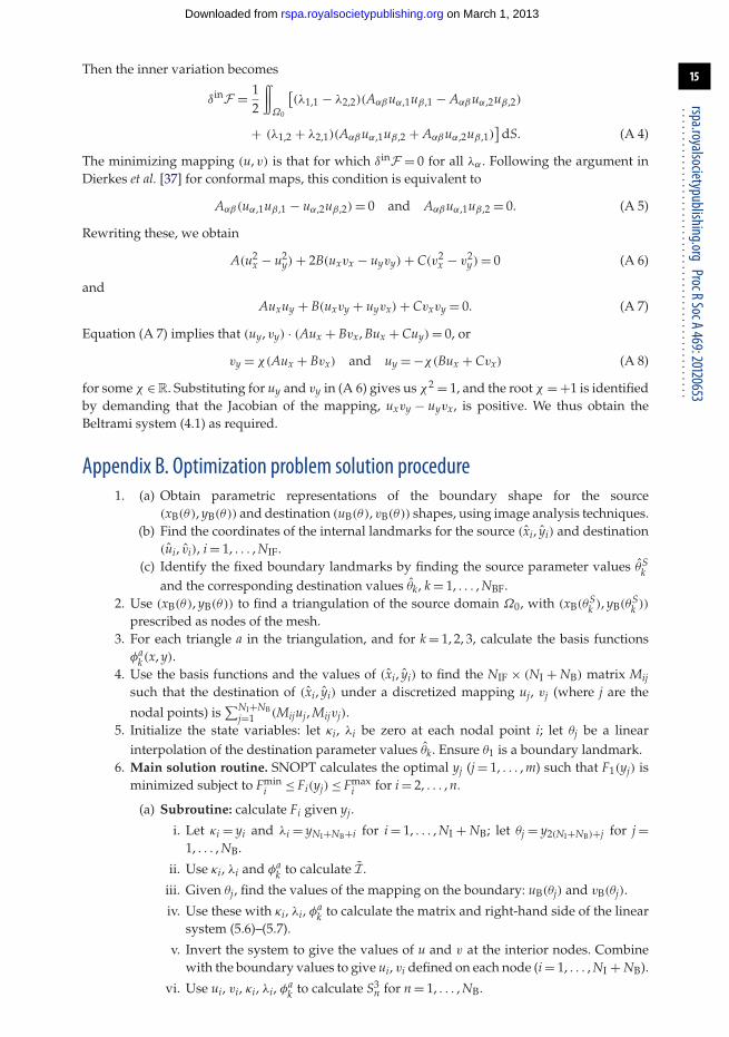
Appendix B. Optimization problem solution procedure1. (a) Obtain parametric representations of the boundary shape for the source

(xB(θ), yB(θ)) and destination (uB(θ), vB(θ)) shapes, using image analysis techniques.(b) Find the coordinates of the internal landmarks for the source (xi, yi) and destination

(ui, vi), i = 1, . . . , NIF.(c) Identify the fixed boundary landmarks by finding the source parameter values θS

kand the corresponding destination values θk, k = 1, . . . , NBF.

2. Use (xB(θ), yB(θ)) to find a triangulation of the source domain Ω0, with (xB(θSk ), yB(θS

k ))

prescribed as nodes of the mesh.3. For each triangle a in the triangulation, and for k = 1, 2, 3, calculate the basis functions

φak(x, y).

4. Use the basis functions and the values of (xi, yi) to find the NIF × (NI + NB) matrix Mijsuch that the destination of (xi, yi) under a discretized mapping uj, vj (where j are the

nodal points) is∑NI+NB

j=1 (Mijuj, Mijvj).5. Initialize the state variables: let κi, λi be zero at each nodal point i; let θj be a linear

interpolation of the destination parameter values θk. Ensure θ1 is a boundary landmark.6. Main solution routine. SNOPT calculates the optimal yj (j = 1, . . . , m) such that F1(yj) is

minimized subject to Fmini ≤ Fi(yj) ≤ Fmax

i for i = 2, . . . , n.

(a) Subroutine: calculate Fi given yj.

i. Let κi = yi and λi = yNI+NB+i for i = 1, . . . , NI + NB; let θj = y2(NI+NB)+j for j =1, . . . , NB.

ii. Use κi, λi and φak to calculate I.

iii. Given θj, find the values of the mapping on the boundary: uB(θj) and vB(θj).

iv. Use these with κi, λi, φak to calculate the matrix and right-hand side of the linear

system (5.6)–(5.7).

v. Invert the system to give the values of u and v at the interior nodes. Combinewith the boundary values to give ui, vi defined on each node (i = 1, . . . , NI + NB).

vi. Use ui, vi, κi, λi, φak to calculate S3

n for n = 1, . . . , NB.

16

rspa.royalsocietypublishing.orgProcRSocA469:20120653

..................................................

on March 1, 2013rspa.royalsocietypublishing.orgDownloaded from

vii. Let

F1 = I,

Fn+1 = S3n for n = 1, . . . , NB,

FNB+1+k =NB+NI∑

j=1

Mkjuj for k = 1, . . . , NIF,

FNB+NIF+1+k =NB+NI∑

j=1

Mkjuj for k = 1, . . . , NIF

and FNB+2NIF+1+j = θj+1 − θj for j = 1, . . . , NB − 1.

(b) Let

Fmini = Fmax

i = 0 for i = 2, . . . , NB+1,

Fmini+NB+1 = Fmax

i+NB+1 = ui for i = 1, . . . , NIF,

Fmini+NB+NIF+1 = Fmax

i+NB+NIF+1 = vi for i = 1, . . . , NIF

and Fmini+NB+2NIF+1 = 0, Fmax

i+NB+2NIF+1 = ∞ for i = 1, . . . , NB − 1.

7. Use the output κi, λi, θk from the SNOPT routine to calculate the mapping ui, vi by solvingthe same linear system as in the subroutine.

References1. Thompson DW. 1917 On growth and form. Cambridge, UK: Cambridge University Press.2. Gould SJ. 1966 Allometry and size in ontogeny and phylogeny. Biol. Rev. 41, 587–638.

(doi:10.1111/j.1469-185X.1966.tb01624.x)3. Richards OW, Riley GA. 1937 The growth of amphibian larvae illustrated by transformed

coordinates. J. Exp. Zool. 77, 159–167. (doi:10.1002/jez.1400770108)4. Lull RS, Gray SW. 1949 Growth patterns in the Ceratopsia. Am. J. Sci. 247, 492–503.

(doi:10.2475/ajs.247.7.492)5. Richards OW. 1955 D’Arcy W. Thompson’s mathematical transformation and the analysis of

growth. Ann. NY Acad. Sci. 63, 456–473. (doi:10.1111/j.1749-6632.1955.tb32103.x)6. Avery GS. 1933 Structure and development of the tobacco leaf. Am. J. Bot. 20, 565–592.

(doi:10.2307/2436259)7. Jacobson AG, Gordon R. 1976 Changes in the shape of the developing vertebrate nervous

system analyzed experimentally, mathematically and by computer simulation. J. Exp. Zool.197, 191–246. (doi:10.1002/jez.1401970205)

8. Medawar PB. 1945 Size, shape, and age. In Essays on growth and form presented to D’ArcyWentworth Thompson (eds WE Le Gros Clark, PB Medawar), pp. 157–187. Oxford, UK: OxfordUniversity Press.

9. Sneath PHA. 1967 Trend-surface analysis of transformation grids. J. Zool. 151, 65–122.(doi:10.1111/j.1469-7998.1967.tb02866.x)

10. Cheverud JM, Richtsmeier JT. 1986 Finite-element scaling applied to sexual dimorphism inrhesus macaque (Macaca mulatta) facial growth. Sys. Zool. 35, 381–399. (doi:10.2307/2413389)

11. Bookstein FL. 1977 The study of shape transformation after D’Arcy Thompson. Math. Biosc.34, 177–219. (doi:10.1016/0025-5564(77)90101-8)

12. Bookstein FL. 1978 Linear machinery for morphological distortion. Comp. Biomed. Res. 11,435–458. (doi:10.1016/0010-4809(78)90002-2)

13. Bookstein FL. 1989 Principal warps: thin-plate splines and the decomposition of deformations.IEEE Trans. Pattern Anal. Machine Intell. 11, 567–585. (doi:10.1109/34.24792)

14. Kent JT, Mardia KV. 1994 The link between kriging and thin-plate splines. In Probability,statistics and optimisation (ed. FP Kelly), ch. 24, pp. 325–339. Chichester, UK: Wiley.

15. Bookstein FL. 1996 Biometrics, biomathematics and the morphometric synthesis. Bull. Math.Biol. 58, 313–365. (doi:10.1007/BF02458311)

17

rspa.royalsocietypublishing.orgProcRSocA469:20120653

..................................................

on March 1, 2013rspa.royalsocietypublishing.orgDownloaded from

16. Grenander U, Miller MI. 1998 Computational anatomy: an emerging discipline. Q. App. Math.56, 617–694.

17. Mumford D, Desolneux A. 2010 Pattern theory. Natick, MA: A.K. Peters.18. Miller MI, Trouvé A, Younes L. 2002 On the metrics and Euler–Lagrange equations

of computational anatomy. Ann. Rev. Biomed. Eng. 4, 375–405. (doi:10.1146/annurev.bioeng.4.092101.125733)

19. Mallarino R, Abzhanov A. 2012 Paths less traveled: evo-devo approaches to investigatinganimal morphological evolution. Ann. Rev. Cell Dev. Biol. 28, 743–763. (doi:10.1146/annurev-cellbio-101011-155732)

20. Gordon R. 2006 Mechanics in embryogenesis and embryonics: prime mover orepiphenomenon? Intl. J. Dev. Biol. 50, 245–253. (doi:10.1387/ijdb.052103rg)

21. Lecuit T, Lenne P-F. 2007 Cell surface mechanics and the control of cell shape, tissue patternsand morphogenesis. Nat. Rev. Mol. Cell Biol. 8, 633–644. (doi:10.1038/nrm2222)

22. Savin T, Kurpios N, Shyer A, Florescu P, Liang H, Mahadevan L, Tabin C. 2011 The growthand form of the gut. Nature 476, 57–62. (doi:10.1038/nature10277)

23. Gerbode S, Puzey J, McCormick A, Mahadevan L. 2012 How the cucumber tendril coils andoverwinds. Science 337, 1087–1091. (doi:10.1126/science.1223304)

24. Goodwin BC. 2000 The life of form. Emergent patterns of morphological transformation. C. R.l’Acad. Sci. Série III, Sciences de la Vie 323, 15–21.

25. Ambrosi D, et al. 2011 Perspectives on biological growth and remodeling. J. Mech. Phys. Solids59, 863–883. (doi:10.1016/j.jmps.2010.12.011)

26. Jones GW, Chapman SJ. 2012 Modeling growth in biological materials. SIAM Rev. 54, 52–118.(doi:10.1137/080731785)

27. Bajcsy R, Lieberson R, Reivich M. 1983 A computerized system for the elastic matching ofdeformed radiographic images to idealized atlas images. J. Comp. Assisted Tomogr. 7, 618–625.(doi:10.1097/00004728-198308000-00008)

28. Christensen GE, Rabbitt RD, Miller MI. 1996 Deformable templates using large deformationkinematics. IEEE Trans. Image Process. 5, 1435–1447. (doi:10.1109/83.536892)

29. Holden M. 2008 A review of geometric transformations for nonrigid body registration. IEEETrans. Med. Imaging 27, 111–128. (doi:10.1109/TMI.2007.904691)

30. Ahlfors LV. 2006 Lectures on quasiconformal mappings, 2nd edn. Providence, RI: AmericanMathematical Society.

31. Tsuchiya T. 2001 Finite element approximations of conformal mappings. Num. Funct. Anal.Optim. 22, 419–440. (doi:10.1081/NFA-100105111)

32. Mastin CW, Thompson JF. 1978 Discrete quasiconformal mappings. Z. Ang. Math. Phys. 29,1–11. (doi:10.1007/BF01797299)

33. Garabedian PR. 1970 A method of canonical coordinates for flow computations. Comm. PureApp. Math. 23, 313–327. (doi:10.1002/cpa.3160230306)

34. Persson P-O, Strang G. 2004 A simple mesh generator in MATLAB. SIAM Rev. 46, 329–345.(doi:10.1137/S0036144503429121)

35. Gill PE, Murray W, Saunders MA. 2005 SNOPT: an SQP algorithm for large-scale constrainedoptimization. SIAM Rev. 47, 99–131. (doi:10.1137/S0036144504446096)

36. Edwards KA, Doescher LT, Kaneshiro KY, Yamamoto D. 2007 A database of wing diversity inthe Hawaiian Drosophila. PLoS ONE 2, e487. (doi:10.1371/journal.pone.0000487)

37. Dierkes U, Hildebrandt S, Sauvigny F. 2010 Minimal surfaces. Berlin, Germany: Springer.