Numerical conformal mappings and capacity computationlib.tkk.fi/Dipl/2009/urn100256.pdf ·...

HELSINKI UNIVERSITY OF TECHNOLOGY

Faculty of Information and Natural Sciences

Tri Quach

Numerical conformal mappings andcapacity computation

Master’s thesis submitted in partial fulfillment of the requirements for the degreeof Master of Science in Technology in Degree Programme in Automation andSystems Technology.

Espoo, November 3, 2009

Supervisor: Professor Timo EirolaInstructor: Ph.D. Antti Rasila

TEKNILLINEN KORKEAKOULU DIPLOMITYÖN

INFORMAATIO- JA LUONNONTIETEIDEN TIEDEKUNTA TIIVISTELMÄ

TEKNILLISEN FYSIIKAN JA MATEMATIIKAN OSASTO

Tekijä: Tri QuachOsasto: Automaatio- ja systeemitekniikan osastoPääaine: Automaation tietämystekniikat (2271)Sivuaine: Laskennallinen tiede ja tekniikka (2254)Työn nimi: Numeeriset konformikuvaukset ja kapasiteettilaskentaProfessuuri: Mat-1, MatematiikkaTyön valvoja: Professori Timo EirolaTyön ohjaaja: FT Antti Rasila

Tiivistelmä:

Tämän diplomityön tarkoituksena on perehdyttää numeerisiin konformiku-vauksiin ja nelikulmion konformisen modulin laskentaan. Konformikuvauksiatutkitaan sekä niiden kytköksistä fysikaalisiin sovellutuksiin, että matemaat-tisesta tärkeydestä. Laskennallista etua saavutetaan kuvaamalla konformisestiyhdesti yhtenäinen alue joko yksikkökiekolle, ylemmälle puolitasolle tai suora-kaiteelle.

Toisaalta kondensaattorin kapasitanssi voidaan karakterisoida nelikulmion kon-formisen modulin avulla. Tässä diplomityössä annamme kaksi tapaa modulinlaskemiseen:

• Schwarz–Christoffelin kuvaukset,

• elementtimenetelmät.

Saatuja tuloksia verrataan sekä keskenään, että tunnettuihin kirjallisuudenanalyyttisiin ja referenssiarvoihin.

Sivumäärä: 100Avainsanat: konformikuvaukset, nelikulmion moduli,numeeriset menetelmät, Schwarz–Christoffelin kuvaus,elementtimenetelmät

Täytetään osastollaHyväksytty: Kirjasto:

iii

HELSINKI UNIVERSITY OF TECHNOLOGY ABSTRACT OF

FACULTY OF INFORMATION AND NATURAL SCIENCES MASTER’ S THESIS

DEPARTMENT OF ENGINEERING PHYSICS AND MATHEMATICS

Author: Tri QuachProgramme: Degree Programme in Automation and Systems TechnologyMajor subject: Knowledge Engineering in Automation (2271)Minor subject: Computational Science and Engineering (2254)Title: Numerical conformal mappings and capacity computationChair: Mat-1, MathematicsSupervisor: Professor Timo EirolaInstructor: Ph.D. Antti Rasila

Abstract:

The purpose of this thesis is to give an introduction to numerical conformalmappings and the computation of a conformal modulus of a quadrilateral.The theory of conformal mapping is studied because of its connections tophysical applications and for its significance in mathematics. The computationaladvantage can be gain by conformally mapping a simply connected domain ontothe unit disk, the upper half plane, or a rectangle.

On the other hand the capacitance of a condenser can be characterized by theconformal modulus of a quadrilateral. In this thesis, we give two ways to com-pute the modulus, namely

• Schwarz–Christoffel mappings,

• finite element methods.

The obtained results are compared to each other and to known analytic andreference values from literatures.

Pages: 100Keywords: conformal mappings, conformal modulus of aquadrilateral, numerical methods, Schwarz–Christoffel map-ping, finite element methods

Department fillsApproved: Library code:

v

Preface

This thesis was done in the Department of Mathematics and Systems Analysis atthe Helsinki University of Technology during the years2008 and2009. Writingthis thesis had been a long journey which was anything but smooth. I would liketo thank my instructor Ph.D. Antti Rasila for his guidance through the obstaclesand for his valuable suggestions and corrections to the thesis. He was the one whointroduced me to this fascinating subject which I otherwisewould not have con-sidered. Also I wish to thank my supervisor professor Timo Eirola for commentson the thesis. Furthermore I like to thank Ph.D. Harri Hakulafor discussionsabout mathematics in general and especially for advice and comments on finiteelement methods. I warmly thank professor Matti Vuorinen for his comments andsuggestions to the work.

Lastly I wish to thank my friends for listening my mathematical jabbering allthese years and for playing and keeping me up-to-date on the Pokémon tradingcard game.

Tri QuachEspoo, November 3, 2009

vii

Contents

Preface vii

List of Symbols xi

1 Introduction 1

2 Preliminaries 52.1 Curves and domains . . . . . . . . . . . . . . . . . . . . . . . . . 52.2 Complex analysis . . . . . . . . . . . . . . . . . . . . . . . . . . 7

2.2.1 Derivative . . . . . . . . . . . . . . . . . . . . . . . . . . 82.2.2 Integral . . . . . . . . . . . . . . . . . . . . . . . . . . . 102.2.3 Winding number and Argument principle . . . . . . . . . 12

2.3 Conformal mappings . . . . . . . . . . . . . . . . . . . . . . . . 132.4 Möbius transformations . . . . . . . . . . . . . . . . . . . . . . . 152.5 Elliptic integrals . . . . . . . . . . . . . . . . . . . . . . . . . . . 192.6 Lebesgue and Sobolev spaces . . . . . . . . . . . . . . . . . . . . 21

3 Riemann mapping theorem 253.1 Preliminary concepts . . . . . . . . . . . . . . . . . . . . . . . . 253.2 Statement and proof . . . . . . . . . . . . . . . . . . . . . . . . . 27

4 Conformal modulus of a quadrilateral 354.1 Definitions of a conformal modulus . . . . . . . . . . . . . . . . 354.2 Properties of a modulus . . . . . . . . . . . . . . . . . . . . . . . 40

5 Schwarz–Christoffel mapping 415.1 Schwarz–Christoffel idea . . . . . . . . . . . . . . . . . . . . . . 415.2 Map from the upper half plane onto a polygon . . . . . . . . . . . 425.3 Map from the upper half plane onto the unit disk . . . . . . . . .44

ix

5.4 Map from the upper half plane onto a rectangle . . . . . . . . . .45

6 Finite element methods 496.1 Variational formulation of Laplace equation . . . . . . . . .. . . 506.2 Finite element mesh . . . . . . . . . . . . . . . . . . . . . . . . . 526.3 Shape functions . . . . . . . . . . . . . . . . . . . . . . . . . . . 566.4 Higher-order finite element methods . . . . . . . . . . . . . . . . 59

7 Numerics of the modulus of a quadrilateral 617.1 Side-length . . . . . . . . . . . . . . . . . . . . . . . . . . . . . 627.2 CRDT . . . . . . . . . . . . . . . . . . . . . . . . . . . . . . . . 627.3 Adaptive finite element methods . . . . . . . . . . . . . . . . . . 647.4 Heikkala–Vamanamurthy–Vuorinen iteration . . . . . . . . .. . 657.5 Crowding . . . . . . . . . . . . . . . . . . . . . . . . . . . . . . 66

8 Numerical results 698.1 Symmetric quadrilateral . . . . . . . . . . . . . . . . . . . . . . . 69

8.1.1 Scaling factor . . . . . . . . . . . . . . . . . . . . . . . . 698.1.2 Nesting levels . . . . . . . . . . . . . . . . . . . . . . . . 708.1.3 Refining vertices . . . . . . . . . . . . . . . . . . . . . . 72

8.2 Modulus of the convex quadrilateral . . . . . . . . . . . . . . . . 738.3 Modulus of the ring domains . . . . . . . . . . . . . . . . . . . . 73

9 Conclusion and further research 77

A Hierarchic shape functions 79

Bibliography 79

x

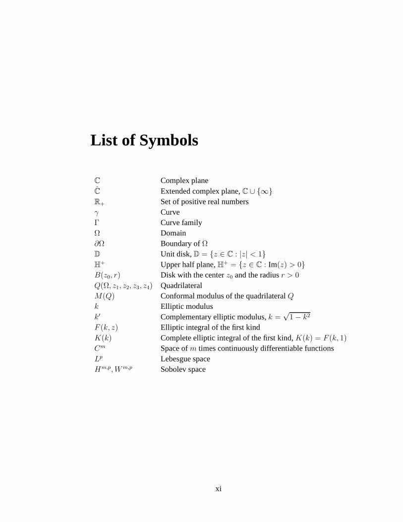
List of Symbols

C Complex planeC Extended complex plane,C ∪ ∞R+ Set of positive real numbersγ CurveΓ Curve familyΩ Domain∂Ω Boundary ofΩD Unit disk,D = z ∈ C : |z| < 1H+ Upper half plane,H+ = z ∈ C : Im(z) > 0B(z0, r) Disk with the centerz0 and the radiusr > 0

Q(Ω, z1, z2, z3, z4) QuadrilateralM(Q) Conformal modulus of the quadrilateralQk Elliptic modulusk′ Complementary elliptic modulus,k =

√1 − k2

F (k, z) Elliptic integral of the first kindK(k) Complete elliptic integral of the first kind,K(k) = F (k, 1)

Cm Space ofm times continuously differentiable functionsLp Lebesgue spaceHm,p,Wm,p Sobolev space

xi

Chapter 1

Introduction

The theory of conformal mappings are studied because of their close relation tophysical applications in, for example, electrostatisticsand aerodynamics, as wellas their theoretical significance in mathematics. In applications numerical com-putations are usually required. For example, the analytical computation of thecapacitance can be carried out only for few condensers. Thisis illustrated by thefollowing simple example. Let us consider a cylindrical condenser, see Figure 1.1.Then the capacitance per unit length is given by

C

L=

2πε

ln (R/r),

whereε is the permittivity factor andL is the length of the cylinder. The con-nection between the capacitance and the conformal modulus of a quadrilateral isshown in Example 4.1.2.

We consider mappings that map conformally simply connecteddomains ontosimplier domains like the unit disk, the upper half plane, orrectangles. In physicalapplications partial differential equations usually arise

−a∆u + b∇u+ cu = f.

By mapping the domain onto simplier one, the computational advantage is clear.In particular, the Laplace equation∆u = 0 is one of the the most important partialdifferential equations in engineering mathematics. For Laplace equations, we mayuse the complex analysis to representf(x+iy) = u(x, y)+iv(x, y), whereu(x, y)andv(x, y) are harmonic functions.

There are many old and new applications of conformal mappings, for examplein cartography. Historically, Mercator’s cylindrical mapprojection was the first

1

2 1. INTRODUCTION

r

R

Figure 1.1: The cross-section of the cylinder.

conformal mapping studied because of this property. It mapsconformally theEarth’s surface onto the plane. The projection distort the area and length near thepoles, for example Greenland and Africa have approximatelythe same size at theprojection, but in the real world, Africa is about10 times as large as Greenland is.Furthermore, in the last century conformal mappings have been used in wide rangeof applications such as integrated and printed circuits, nuclear reactors, airfoils,pattern recognitions, and condensers [SL]. Applications on vortex dynamics havebeen studied in [SC] and further applications to fluids and flows are described in[Cro1, Cro2, Cro3, TD].

In this thesis we are interested on a quantity called the conformal modulus ofa quadrilateral. For computations we use mainly two different approaches

1. Schwarz–Christoffel mappings,

2. finite element methods.

The former methods give the conformal modulus as well as the auxiliary confor-mal mapping of the quadrilateral onto a rectangle.

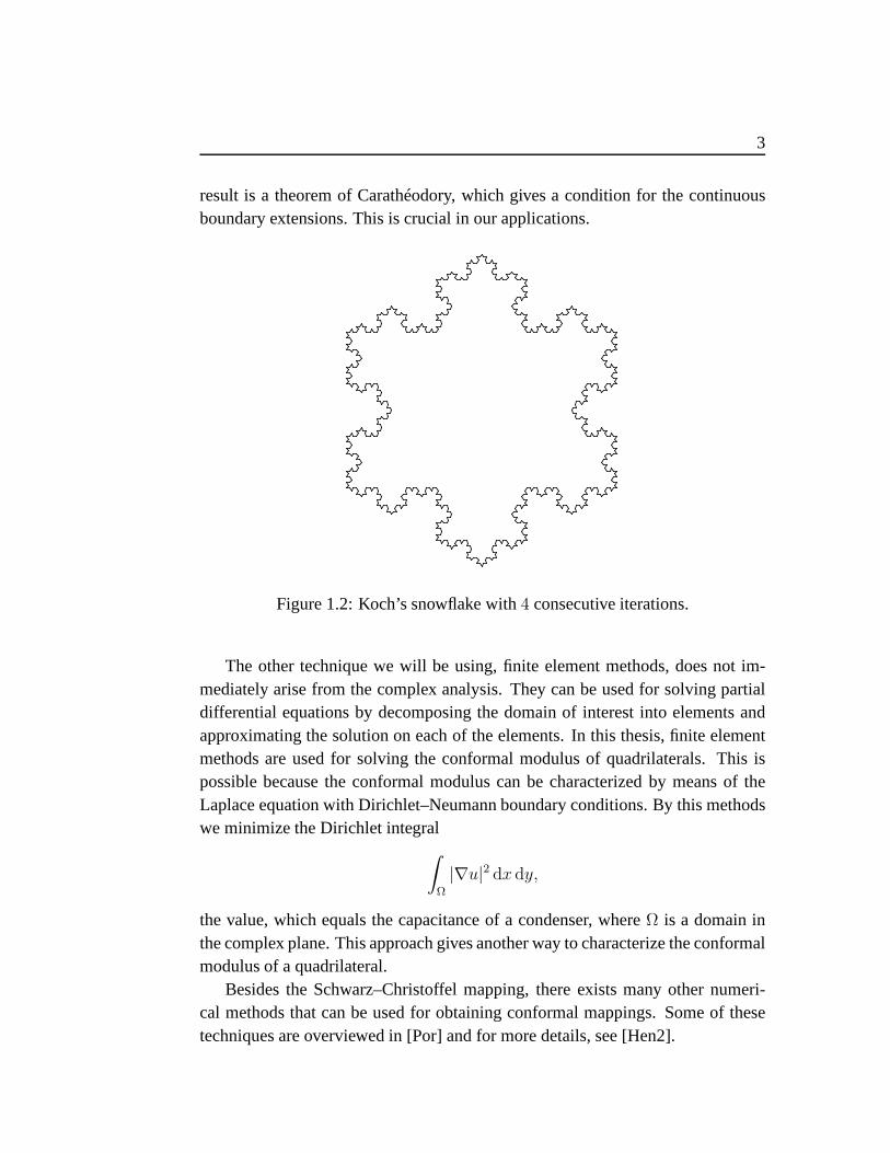
Schwarz–Christoffel mappings are closely related to the Riemann mappingtheorem which states that any simply connected domain except the whole complexplane can be map onto the unit disk. It is noteworthy that evensimply connecteddomains with, for example, fractal boundaries such as Koch’s snowflake (Figure1.2) can be conformally mapped onto the unit disk [Pom]. Another important

3

result is a theorem of Carathéodory, which gives a conditionfor the continuousboundary extensions. This is crucial in our applications.

Figure 1.2: Koch’s snowflake with4 consecutive iterations.

The other technique we will be using, finite element methods,does not im-mediately arise from the complex analysis. They can be used for solving partialdifferential equations by decomposing the domain of interest into elements andapproximating the solution on each of the elements. In this thesis, finite elementmethods are used for solving the conformal modulus of quadrilaterals. This ispossible because the conformal modulus can be characterized by means of theLaplace equation with Dirichlet–Neumann boundary conditions. By this methodswe minimize the Dirichlet integral

∫

Ω

|∇u|2 dx dy,

the value, which equals the capacitance of a condenser, where Ω is a domain inthe complex plane. This approach gives another way to characterize the conformalmodulus of a quadrilateral.

Besides the Schwarz–Christoffel mapping, there exists many other numeri-cal methods that can be used for obtaining conformal mappings. Some of thesetechniques are overviewed in [Por] and for more details, see[Hen2].

4 1. INTRODUCTION

This thesis is organized as follows. In Chapter 2 we give background materialto understand this thesis. In Chapter 3 we state the Riemann mapping theorem andgive a proof through a normal family argument. Definitions and properties of theconformal modulus of quadrilaterals are given in Chapter 4.In Chapter 5 we studythe Schwarz–Christoffel mappings which can be used for mapping a polygonaldomain onto the unit disk, the upper half plane, or a rectangle. The theory of finiteelement methods is developed in Chapter 6. Numerical methods related to theSchwarz–Christoffel mapping and finite element methods arestudied in Chapter7. Finally, in Chapter 8, we consider examples of quadrilaterals and compute themodulus by both the Schwarz–Christoffel toolbox [Dri] andhp-version of finiteelement methods. The results are compared to each other and to known referenceresults. In Chapter 9 we discuss about the results obtained in Chapter 8 and wegive some ideas for further research.

This thesis is closely related to earlier work in the same research group, seefor example theses [Num, Vuo, Yrj] and research papers [BSV,DuVu, HRV, RV].

Chapter 2

Preliminaries

In this chapter we give basic definitions and results used in the theory of conformalmappings. Presented results are well known, so the reader familiar with the topicmay glance through it quickly and begin with the next chapter, referring to thischapter when necessary.

2.1 Curves and domains

Definition 2.1.1. (Curve)A curve is a continuous functionγ : [a, b] → C, whereC = C ∪ ∞ is theextended complex plane, the so called one point compactification of C.

A curve is said to besmoothif it is continuously differentiable andγ(t) 6= 0.We denote a set of curves byΓ and call it acurve family.

Definition 2.1.2. (Length of a curve)Let γ be a curve,γ : [a, b] → C, and letTk : a = t0 < t1 < · · · < tk = b bea partition of the closed interval[a, b]. The setγ([a, b]) is called thelocusof γ.Then, by denotingγi = γ(ti), thelengthof the curveγ is defined by the supremumof sums

l(γ) = supTk

k∑

i=1

|γi − γi−1| .

If the curveγ is piecewise differentiable, then we can define, alternatively, thelength of the curve by

l(γ) =

∫ b

a

|y′(t)| dt.

5

6 2. PRELIMINARIES

A curveγ is said to berectifiableif its length is finite. A curveγ with para-metric interval[a, b] such thatγ(a) = γ(b) is called aclosed curve. That is, thestarting point and the end point ofγ are the same. Furthermore,γ is said to besimpleif it does not intersect itself, that is, ifγ(c) 6= γ(d), for all c 6= d, wherec, d ∈ (a, b). Note that the exceptionγ(a) = γ(b) is allowed. Ifγ is both simpleand closed, then it is called aJordan curve[Pon, p. 117].

Simple, closed Not simple, closed Simple, open Not simple, open

Figure 2.1: Different types of curves.

Definition 2.1.3. (Domain)A domainΩ is a non-empty open connected set inC. In particular, a domainΩ ispath-wise connected, that is for each pair of pointsz1 andz2 in Ω can be connectedwith a curveγ such that theγ lies entirely inΩ.

A domain together with some, none, or all of its boundary points is called aregion. The closure of a domainΩ is denoted byΩ and is the union of the domainΩ and the boundary curve∂Ω. A domainΩ is said to besimply connectedifits complement with respect to the extended plane is connected. For reasons ofconvenience we do not consider the whole complex planeC as simply connected.If Ω is not simply connected, then we say thatΩ is multiply connected. A domainΩ bounded by a Jordan curve is called aJordan domain. Note that every Jordandomain is simply connected.

Definition 2.1.4. (Generalized quadrilateral)A generalized quadrilateralis a Jordan domainΩ with four separate boundarypointsz1, z2, z3, andz4 given in positive order on the boundary curve∂Ω of Ω.These points are called vertices of the generalized quadrilateral. They divide∂Ωinto four curvesγ1, γ2, γ3, andγ4 which are called the sides of the generalizedquadrilateral and denoted by(z1, z2), (z2, z3), (z3, z4), and(z4, z1), respectively.

2.2. COMPLEX ANALYSIS 7

Simply connected Not a domain Multiply connected

Figure 2.2: Different types of sets.

In this case, when we traverse∂Ω such thatΩ is on the left-hand side, thepointsz1, z2, z3, andz4 occur in this order. We denote a generalized quadrilateralbyQ(Ω; z1, z2, z3, z4).

γ4

γ1

γ2

γ3

Ω

z1

z2

z3

z4

Figure 2.3: A generalized quadrilateralQ(Ω; z1, z2, z3, z4).

If the sidesγk, wherek = 1, 2, 3, 4, are line segments, then the generalizedquadrilateral will be a quadrilateral in the usual geometric sense. In what fol-lows the word quadrilateral is used to describe both geometric and generalizedquadrilaterals.

2.2 Complex analysis

The origin of complex numbers lies in the problem of finding roots of polynomialequations. Already in the early16th century Cardano, Tartaglia, and Ferro founda long sought general solution for the cubic equation. In some cases Cardano–Tartaglia–Ferro formula gives a solution which seemingly looks like a complexnumber even though the solution is, for example a positive real number. This

8 2. PRELIMINARIES

puzzled Cardano who acknowledged the existence of these bizarre numbers eventhough he could not make any use of them. Bombelli showed in1572 that the rootsof a negative number have a great utility by manipulating a seemingly complexsolution obtained by Cardano–Tartaglia–Ferro formula into a real number solu-tion. In the18th century Euler introduced the modern notationi =

√−1 [Lau, pp.

64–69].We assume that the reader is familiar with complex numbers. If this is not the

case, please see, for example, [Ahl1, Gam, MH, NP, Pon] for basic concepts ofcomplex numbers.

2.2.1 Derivative

Suppose that for every valuez in a domainΩ there corresponds a definite complexvaluew. Then the functionf : z 7→ w is said to be a complex function defined inΩ. A functionf(z) is said to besingle-valuedif f(z) satisfies

f(z) = f(z(r, ϕ)) = f(z(r, ϕ + 2π)).

Otherwise,f(z) is said to bemultiple-valued.

Definition 2.2.1. (Derivative)A complex functionf(z) defined in a domainΩ is differentiableat a pointz0 ∈ Ω

if the limit

limz→z0

f(z) − f(z0)

z − z0= lim

∆z→0

f(z0 + ∆z) − f(z0)

∆z

exists and is independent of the path along which∆z → 0. The limit is denotedby f ′(z0) and is called the complex derivative of the functionf(z) at the pointz0.

The complex derivative shares many of the properties of the real derivative.See [Ahl1] for a further reference.

Definition 2.2.2. (Analytic function)A function f(z) is said to beanalytic, or holomorphic, at a pointz0 ∈ C if it isdifferentiable at every point of some neighborhood of the point z0. Similarly, afunctionf(z) is said to be analytic in a setE if it is differentiable at every pointof some open setΩ such thatE ⊂ Ω.

A function f(z), which is analytic in the whole complex planeC is called anentire function. Suppose that a functionf(z) is analytic in a neighborhood of apoint z0, except perhaps atz0 itself. If lim

z→z0

f(z) = ∞, the pointz0 is said to


be apole of f(z), and we setf(z0) = ∞. A function f(z) which is analyticin a domainΩ, except for poles, is said to bemeromorphicin Ω. Furthermore,a meromorphic functionf(z) at a pointz0 is said to have an orderN at z0 iff(z) = (z − z0)

Ng(z) for some analytic functiong(z) at z0 such thatg(z0) 6= 0.

Determining whether a given functionf(z) is analytic or not directly from thedefinition is not usually practical. Fortunately, theCauchy–Riemann equationsgive us a convenient characterization of analytic functions.

Theorem 2.2.3.(Cauchy–Riemann equations)Let a functionf(z) = u(x, y)+ iv(x, y) be defined and continuous in some neigh-borhood of a pointz0 = x0 + iy0 and differentiable atz0. Thenf(z) is analyticif partial derivatives1 of u(x, y) andv(x, y) exists atz0 and satisfy the Cauchy–Riemann equations

∂u

∂x=∂v

∂y,

∂u

∂y= −∂v

∂x(2.1)

in the neighborhood ofz0.

Furthermore, iff(z) is analytic in a domainΩ, thenf(z) satisfies the Cauchy–Riemann equations for every pointz ∈ Ω.

Definition 2.2.4. (Harmonic function) [Ahl1, p. 162]A real-valued functionu(z) = u(x, y) defined and single-valued in a domainΩ,is said to beharmonicin Ω if it is continuous together with its partial derivativesof the first two orders and satisfiesLaplace’s equation

∆u = uxx + uyy = 0.

It is easy to see that for analytic function ,f(z) = u(z) + iv(z), f : Ω → C,the functionsu(z) and v(z) are harmonic inΩ. A function v(z) = v(x, y) iscalled aconjugate harmonic functionfor a harmonic functionu(z) in Ω wheneverf(z) = u(z) + iv(z) is analytic inΩ.

To construct a conjugate harmonic functionv(z), we use the information thatf(z) is analytic. In particular,f(z) satisfies the Cauchy-Riemann equations (2.1).Sov(z) can be expressed by

v(x, y) =

∫

ux(x, y) dy + C(x), (2.2)

1Notation:ux(x, y) = ∂u

∂x(x, y).

10 2. PRELIMINARIES

whereC(x) is a function ofx alone to be determined. Differentiating (2.2) withrespect tox, we will get

vx(x, y) =∂

∂x

∫

ux(x, y) dy +d

dxC(x)

C-R⇒ −uy(x, y) =∂

∂x

∫

ux(x, y) dy +d

dxC(x).

The functionC(x) can now be solved from the last equation by integrating withrespect ofx. Note that the conjugate harmonic functionv(z) is unique up to anaddition of a real constant.

We also use the following result:

Theorem 2.2.5.(Liouville’s Theorem) [Ahl1, p. 122]A bounded and entire function is constant.

2.2.2 Integral

Arithmetic operations and calculus of differentiations generalize from the real to acomplex variable without difficulties. But defining acomplex integral, also knownascontour integral, the transition is not as straightforward as it could be imagined.For some historical remarks see [Lau, pp. 73–75].

Let a curveγ and a partitionTk of an interval[a, b] be as in Definition 2.1.2.For each interval(ti−1, ti), wherei = 1, · · · , k, we choose an arbitrary pointt = τi. Suppose thatf(z) is defined and continuous onγ. Settingξi = γ(τi) andγi = γ(ti), we consider the expression

ΣTk=

k∑

i=1

f(ξi)(γi − γi−1). (2.3)

Suppose that the length of each interval(ti−1, ti) of the partitionTk is bounded,then the sum (2.3) will tend to a finite limit when the partitionTk is refined so thatk → ∞ and the length of the longest interval|ti − ti−1|, i = 1, 2, · · · , k, tends tozero. ΣTk

tends to a limit which is called the integral off(z) along the curveγ

and denoted by∫

γ

f(z) dz. Thus,

∫

γ

f(z) dz = supTk

k∑

i=1

f(ξi)(γi − γi−1).


The value of the integral is independent of the way the refining process ofTk

is carried out [Neh, pp. 81–83], [NP, pp. 108–109]. For a proof, see [NP, pp.109–110].

| | | | | | |a b|ti−1 ti

|τi γ

|| |

||

| |

|

γa

γb

γ i−1γi|

ξi

Figure 2.4: Partition of a curve in a complex integral.

If the curveγ is a line segment[a, b] of the real line, then the integral of thecontinuous complex valued functionf(t) = u(t) + iv(t) is defined by

∫ b

a

f(t) dt =

∫ b

a

u(t) dt+ i

∫ b

a

v(t) dt.

Suppose that a curveγ is piecewise differentiable with a parametrizationγ = γ(t),a ≤ t ≤ b. If the functionf(z) is defined and continuous onγ thenf(γ(t)) iscontinuous as well. Then we define the integral off(z) over the curveγ by

∫

γ

f(z) dz =

∫ b

a

f(γ(t)) γ′(t) dt.

The complex integral has the usual properties of the real integral. For furtherreference see [Ahl1].

For analytic functions we have following theorem.

Theorem 2.2.6.(Cauchy’s integral theorem) [Ahl1, p. 109]Let Ω be simply connected domain and suppose thatf(z) is analytic onΩ. Then

∫

∂Ω

f(z) = 0.

By Theorem 2.2.6, the contour integral of the analytic function f(z) is pathindependent.

12 2. PRELIMINARIES

2.2.3 Winding number and Argument principle

The concepts of winding numbers and argument principles tell us how many timesthe given curveγ wind up a given pointz. The theory is based on calculus ofresidues and Cauchy theorems. We will only give the necessary definitions andtheorems to understand the proof of Theorem 4.1.3.

Definition 2.2.7. (Branch) [Pon, p. 105]SupposeF (z) is a multiple-valued function defined inΩ. A branchof F (z) is asingle-valued analytic functionf(z) in some domainU ⊂ Ω obtained fromF (z)

in such a way that at each point ofU , f(z) assumes exactly one of the possiblevalues ofF (z).

Definition 2.2.8. (Winding number) [Ahl1, p. 115]Let γ be a piecewise smooth closed curve. Suppose a pointa 6∈ γ. Then thewinding numberof the pointa respect to the curveγ is given by

n(γ, a) =1

2πi

∫

γ

dz

z − a.

The winding number can be interpreted intuitively as the number of timesγwraps around the pointa in positive order. The following theorem states all thepossible winding numbers for a Jordan curve.

Theorem 2.2.9.(Jordan curve theorem) [NP, pp. 178–179]A Jordan curveγ separates the complex plane into two domainsΩ1 andΩ2, bothof which are bounded byγ. One of the domains is bounded and the other isunbounded. Without loss of generality we may assume thatΩ1 is bounded andΩ2

is unbounded.Then the winding number of each pointa ∈ Ω2 respect ofγ is zero and the

winding number of each pointa ∈ Ω1 respect ofγ is either+1 or −1 dependingon the orientation ofγ, positive or negative, respectively.

In calculations of the argument principle, we will be using the above propertyof the winding number.

Theorem 2.2.10.(Argument principle) [Gam, pp. 224–225]Let Ω be bounded domain with a piecewise smooth boundary∂Ω, and letf(z) bea meromorphic function onΩ that extends analytically on∂Ω, such thatf(z) 6= 0

on∂Ω. Then1

2πi

∫

∂Ω

f ′(z)

f(z)dz = N0 −N∞,

2.3. CONFORMAL MAPPINGS 13

whereN0 andN∞ denote, respectively, the numbers of zeros and poles off(z) inΩ, counted according the orders.

The integral in Theorem 2.2.10 is often referred to as alogarithmic integraloff(z) alongγ. In case of a Jordan curve the Argument principle can be stated asfollowing theorem:

Theorem 2.2.11.(Argument principle for a Jordan curve) [Hen1, p. 278]Let f(z) be analytic in a simply connected domainΩ and letγ be a positivelyoriented Jordan curve inΩ not passing through any zero off(z). Then the numberof zeros off(z) in the interior ofγ, each zero counted according to its multiplicity,equals the winding number of the image curvef(γ) with respect to0.

2.3 Conformal mappings

The history of conformal mappings can be dated back to the 16th century. In1569

Mercator presented a cylindrical map projection which is a conformal mappingfrom a sphere onto the plane. It was not until1820 that Gauss gave the formaldefinition to conformal mappings. Thus, Mercator preceded Gauss by nearly threecenturies.

A heuristic way to define a conformal mapping is the following. A mappingf : z 7→ w is said to beconformalat z0 if it preserves angles and their orientationbetween smooth curves throughz0. Obviously, such mappings are very useful incartography.

More precisely, letf be an analytic function in the domainΩ and letz0 be apoint inΩ. If f ′(z0) 6= 0, thenf can be expressed by

f(z) = f(z0) + f ′(z0)(z − z0) + η(z)(z − z0),

whereη(z) → 0 asz → z0. Wheneverz is in a sufficiently small neighborhoodof z0, the transformationw = f(z) can be approximated by

S(z) = f(z0) + f ′(z0)(z − z0)

= f(z0) − f ′(z0)z0 + f ′(z0)z.

Here the mappingS(z) can be represented as a following composite map. Firstapply a rotation of the plane through the angleArgf ′(z0), then a scaling by thefactor|f ′(z0)|. Finally use the translationf(z0) − f ′(z0)z0.

14 2. PRELIMINARIES

Let γ(t) be a smooth curve that passes through a pointz0 andf ′(z0) 6= 0.Then the tangent to the curve

γ(t) = (f γ)(t),

atw0 = f(z0) is given by

(f γ)′(t0) = f ′(z0)γ′(t0).

A mappingf : Ω → C is said to be conformal atz0 ∈ Ω if, for any two parameter-ized curvesγ1 andγ2 intersecting at the pointz0 = γ1(t0) = γ2(t0) with non-zerotangents, the following conditions hold:

(i) the transformed curvesγ1 = f γ1 andγ2 = f γ2 have non-zero tangentsat the pointt0, and

(ii) the angle betweenγ′1(t0) = (f γ1)′(t0) andγ′2(t0) = (f γ2)

′(t0) is sameas the angle betweenγ′1(t0) andγ′2(t0).

If the functionf(z) is conformal at each point of a domainΩ, thenf(z) is said tobe locally conformal inΩ [Pon, pp. 194–195]. Iff(z) is also a bijection,f(z) isa conformal mapping inΩ.

y

xγ′1

γ′2

α

z0

z–plane

v

u

γ′1

γ′2α

w0

w–plane

f(z)

Figure 2.5: An illustration of a conformal map.

Example 2.3.1.Let us consider a mapping

f(z) =

(1 + z

1 − z

)2

,

2.4. MÖBIUS TRANSFORMATIONS 15

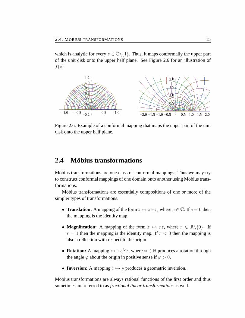
which is analytic for everyz ∈ C\1. Thus, it maps conformally the upper partof the unit disk onto the upper half plane. See Figure 2.6 for an illustration off(z).

-1.0 -0.5 0.5 1.0-0.2

0.2

0.4

0.6

0.8

1.0

1.2

-2.0-1.5-1.0-0.5 0.5 1.0 1.5 2.0

0.5

1.0

1.5

2.0

Figure 2.6: Example of a conformal mapping that maps the upper part of the unitdisk onto the upper half plane.

2.4 Möbius transformations

Möbius transformations are one class of conformal mappings. Thus we may tryto construct conformal mappings of one domain onto another using Möbius trans-formations.

Möbius transformations are essentially compositions of one or more of thesimpler types of transformations.

• Translation: A mapping of the formz 7→ z+ c, wherec ∈ C. If c = 0 thenthe mapping is the identity map.

• Magnification: A mapping of the formz 7→ rz, wherer ∈ R\0. Ifr = 1 then the mapping is the identity map. Ifr < 0 then the mapping isalso a reflection with respect to the origin.

• Rotation: A mappingz 7→ eiϕz, whereϕ ∈ R produces a rotation throughthe angleϕ about the origin in positive sense ifϕ > 0.

• Inversion: A mappingz 7→ 1z

produces a geometric inversion.

Möbius transformations are always rational functions of the first order and thussometimes are referred to asfractional linear transformationsas well.

16 2. PRELIMINARIES

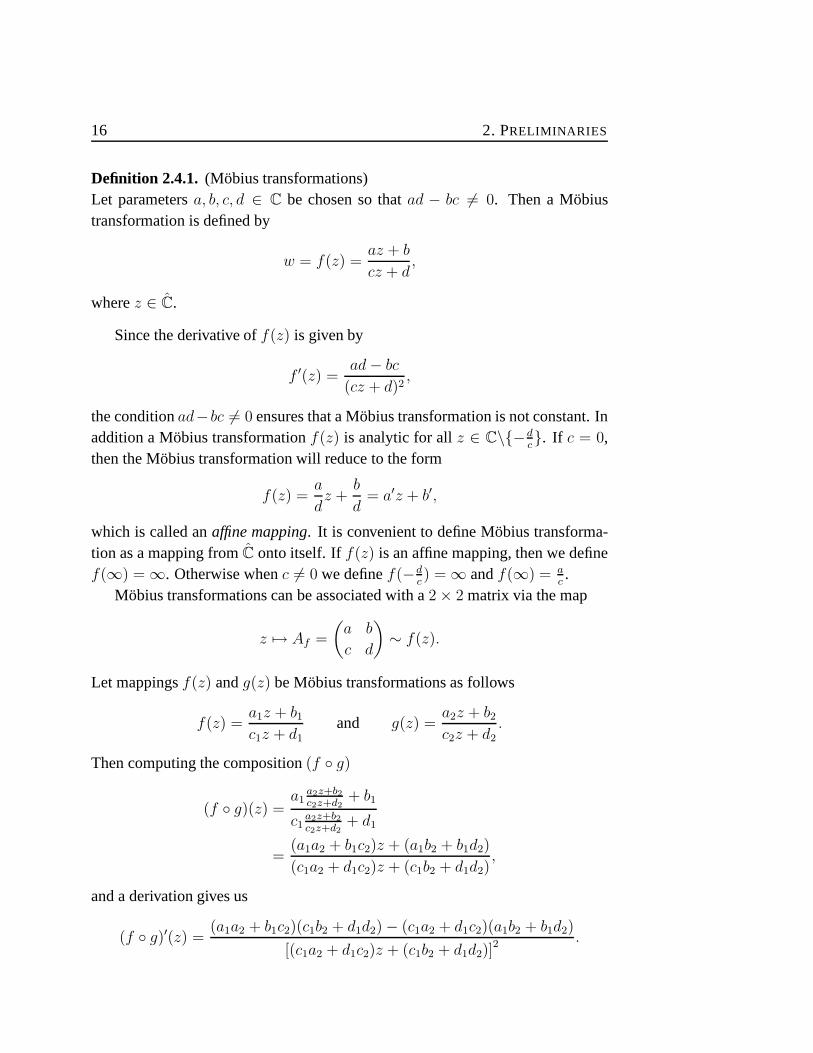
Definition 2.4.1. (Möbius transformations)Let parametersa, b, c, d ∈ C be chosen so thatad − bc 6= 0. Then a Möbiustransformation is defined by

w = f(z) =az + b

cz + d,

wherez ∈ C.

Since the derivative off(z) is given by

f ′(z) =ad− bc

(cz + d)2,

the conditionad− bc 6= 0 ensures that a Möbius transformation is not constant. Inaddition a Möbius transformationf(z) is analytic for allz ∈ C\−d

c. If c = 0,

then the Möbius transformation will reduce to the form

f(z) =a

dz +

b

d= a′z + b′,

which is called anaffine mapping. It is convenient to define Möbius transforma-tion as a mapping fromC onto itself. Iff(z) is an affine mapping, then we definef(∞) = ∞. Otherwise whenc 6= 0 we definef(−d

c) = ∞ andf(∞) = a

c.

Möbius transformations can be associated with a2 × 2 matrix via the map

z 7→ Af =

(a b

c d

)

∼ f(z).

Let mappingsf(z) andg(z) be Möbius transformations as follows

f(z) =a1z + b1c1z + d1

and g(z) =a2z + b2c2z + d2

.

Then computing the composition(f g)

(f g)(z) =a1

a2z+b2c2z+d2

+ b1

c1a2z+b2c2z+d2

+ d1

=(a1a2 + b1c2)z + (a1b2 + b1d2)

(c1a2 + d1c2)z + (c1b2 + d1d2),

and a derivation gives us

(f g)′(z) =(a1a2 + b1c2)(c1b2 + d1d2) − (c1a2 + d1c2)(a1b2 + b1d2)

[(c1a2 + d1c2)z + (c1b2 + d1d2)]2 .

2.4. MÖBIUS TRANSFORMATIONS 17

Then by simplifying the numerator, we have

(a1a2 + b1c2)(c1b2 + d1d2) − (c1a2 + d1c2)(a1b2 + b1d2)

= a1a2d1d2 + b1c2c1b2 − c1a2b1d2 + d1c2a1b2

= (a1d1 − b1c1)(a2d2 − b2c2). (2.4)

Sincef(z) andg(z) are Möbius transformations, the factors in (2.4) are not zero.This implies that a composition of Möbius transformations is a Möbius trans-formation as well. In addition the inverse of a Möbius transformation is also aMöbius transformation and is given by

f−1(w) =dw − b

−cw + a.

The composition and the inverse of Möbius transformations correspond to productand inverse of the matrices, respectively. The analogy is following, the derivativeof a Möbius transformationf ′(z) 6= 0 if and only if thedet(Af) 6= 0.

Möbius transformations map circles inC onto circles inC, where a straightline is considered as a circle with an infinite radius [Gam, pp. 63–66], [Pon, pp.200–206]. In particular we have Möbius transformations which map the unit diskonto itself.

Lemma 2.4.2. (Mapping of the unit disk onto itself) [Kre, p. 740]The mapping

w =z − z0z0z − 1

,

where|z0| < 1 maps the unit disk onto the unit disk such that the pointz0 mapsonto the origin.

Proof: We take|z| = 1 and calculate

|z − z0| = |z − z0|= |z| · |z − z0|= |1 − z0z|= |z0z − 1|.

Hence

|w| =|z − z0||z0z − 1| = 1,

so that the unit circle maps onto the unit circle. Noting thatz0 maps onto theorigin, implies the claim [Kre, p. 740].

18 2. PRELIMINARIES

Example 2.4.3.Let z0 = 12. Then we have

w =2z − 1

z − 2.

In Figure 2.7 we have an illustration of the above mapping.

-1.0 -0.5 0.5 1.0

-1.0

-0.5

0.5

1.0

-1.0 -0.5 0.5 1.0

-1.0

-0.5

0.5

1.0

Figure 2.7: Mapping of the unit disk onto the unit disk.

Definition 2.4.4. (Cross ratio) [Ahl1, p. 78]Fix pointsz1, z2, z3, z4 ∈ C. Then across ratio(z1, z2, z3, z4) is defined by

(z1, z2, z3, z4) =(z4 − z2)(z1 − z3)

(z4 − z3)(z1 − z2).

By the cross ratio, we may construct a Möbius transformationas follows

Theorem 2.4.5. If z1, z2, z3 ∈ C andw1, w2, w3 ∈ C such thatwj = f(zj),j = 1, 2, 3. Then the Möbius transformationw = f(z) can be solved from thecross ratio

(w − w2)(w1 − w3)

(w − w3)(w1 − w2)=

(z − z2)(z1 − z3)

(z − z3)(z1 − z2).

This is true, because the cross ratio is invariant under Möbius transformations[Ahl1, p. 79].

2.5. ELLIPTIC INTEGRALS 19

2.5 Elliptic integrals

There is a vast number of interesting integrals that cannot be expressed in termsof elementary functions. One type of such integrals is knownaselliptic integrals.Such integrals arise from many elementary questions in the natural science. Forexample whenKepler’s lawsbecame known, the first natural aim was to computethe orbit of a planet. Wallis attempted to compute the arc length of an ellipse in1655. Series expansion for elliptic integrals were given by Newton and Euler.

Elliptic integrals were extensively studied by Legendre, Gauss, Abel and Ja-cobi in the early19th century. Legendre showed that every elliptic integral can bereduced by a suitable substitution to one of the three normalforms. These normalforms are called elliptic integral of the first, second and third kind [Cay]. We areonly interested in the elliptic integrals of the first kind, because these provide away to conformally map the upper half plane onto a rectangle.

Definition 2.5.1. (Elliptic integral of the first kind) [Cay, pp. 2–3]Theelliptic integral of the first kindis defined by

F (k, z) =

∫ z

0

dζ√

(1 − ζ2)(1 − k2ζ2),

for 0 < k < 1, where the parameterk is called theelliptic modulus. The comple-mentary elliptic modulus is given byk′ =

√1 − k2.

Substitutingz = sinφ andζ = sin θ, we will get

F (k, sinφ) =

∫ sinφ

0

cos θ dθ√

(1 − sin2 θ)(1 − k2 sin2 θ).

By the identitycos2 θ = 1 − sin2 θ, we eliminate the cosine term and the ellipticintegral of the first kind can also be expressed by

F (k, sinφ) =

∫ sinφ

0

dθ√

1 − k2 sin2 θ,

whereφ is called the amplitude. If the integral is taken up to the amplitude π2, then

it is called the complete elliptic integral of the first kind.

20 2. PRELIMINARIES

Definition 2.5.2. (Complete elliptic integral of the first kind) [Cay, p. 4]Thecomplete elliptic integral of the first kindis defined by

K(k) = F (k, 1) =

∫ 1

0

dζ√

(1 − ζ2)(1 − k2ζ2)

=

∫ π2

0

dθ√

1 − k2 sin2 θ.

for 0 < k < 1, where the parameterk is the elliptic modulus.

The complete complementary elliptic integral of the first kind is denoted by

K ′(k) = K(k′).

The inverse of the elliptic integrals is called Jacobi’s elliptic functions. To simplifythe notation we give a following definition.

Definition 2.5.3. (Jacobi’s elliptic sine function) [Cay, p. 8]Let u = F (k, z). Then theJacobi’s elliptic sine functionsn(u, k) is defined by

sn(u, k) = z.

Jacobi’s elliptic sine function maps conformally a rectangle onto upper halfplane. This result is proved in Section 5.4.

-2.0 -1.5 -1.0 -0.5 0.5 1.0 1.5 2.0

-0.5

0.5

1.0

1.5

2.0

-2.0 -1.5 -1.0 -0.5 0.5 1.0 1.5 2.0

-0.5

0.5

1.0

1.5

2.0

Figure 2.8: Example of a conformal mapping that maps a rectangle onto the upperhalf plane.

2.6. LEBESGUE ANDSOBOLEV SPACES 21

2.6 Lebesgue and Sobolev spaces

In finite element applications often arise situations wherethe functions in gen-eral are, strictly speaking, not differentiable, but can bewell approximated withdifferentiable functions.

Sobolev spaces are vector spaces whose elements are functions defined ondomain ofRn and whose partial derivatives satisfy certain integrability properties.A solution of partial differential equations are sought from Sobolev spaces.

We assume that the reader is familiar with basic concepts of anorm, theLebesgue measure, and Lebesgue integration, for a reference see [Rud1, Rud2].Following definitions and theorems are given inR2 even though generalizationsto higher dimensions could be done, naturally.

Definition 2.6.1. (Compact support) [AF, p. 2]SupposeΩ ⊂ R2 is non-empty. Thesupportof u is defined by

supp(u) = x ∈ Ω : u(x) 6= 0.

We sayu has acompact supportin Ω if supp(u) ⊂ Ω andsupp(u) is compact.

In Rn, compactness is equivalent to closedness and boundedness.This resultis known as the Heine–Borel Theorem. For a proof, see [Rud1, p. 40].

Definition 2.6.2. (Space of continuous function) [AF, p. 10]Let Ω be a domain. For any non-negative integerm let Cm(Ω) denote the vectorspace consisting of all functionsψ which, together with their partial derivativesDαψ of orders|α| ≤ m, are continuous onΩ, where

Dαψ =∂α1

∂α1x

∂α2

∂α2yψ,

andα = (α1, α2) is a pair of non-negative integersα1, α2 and|α| = α1 + α2 iscalled a degree ofα.

We abbreviateC0(Ω) = C(Ω) andC∞(Ω) =

∞⋂

m=0

Cm(Ω). The family of func-

tions of spacesC(Ω) andC∞(Ω) that have a compact support inΩ are denoted byC0(Ω) andC∞

0 (Ω), respectively.

Definition 2.6.3. (Lp–norm) [Rud2, p. 65]Let E ⊂ R

2 be a Lebesgue measurable set and letf : E → [−∞,∞] be a

22 2. PRELIMINARIES

Lebesgue measurable function. If1 ≤ p < ∞, then theLp–norm of f is de-fined by

‖f‖p =

(∫

E

|f(x, y)|p dx dy

)1/p

.

In some situations when confusion about domains may occur wewrite ‖ · ‖p,E

instead of‖ · ‖p. Also the norm is denoted by‖ · ‖Lp(E) if there is a confusionabout the actual space.

Definition 2.6.4. (Lebesgue space) [AF, pp. 23]Let p be a positive real number. We denote byLp(Ω) the class of all measurablefunctionsf(x, y) defined on domainΩ for which

‖f‖p <∞.

Note thatL1(Ω) is a family of functions which are Lebesgue integrable onΩ.For p ∈ [1,∞) the spaceLp(Ω) is not a normed space in a classical sense, since‖f‖p = 0 does not imply thatf ≡ 0. For this reason, we defineLp(Ω) as thespace of equivalence classes

f ∼ g ⇔ f = g, almost everywhere onΩ.

Then it follows thatLp(Ω) is a normed space [Rud2, pp. 65–69].Suppose a functionu is defined almost everywhere on a domainΩ and suppose

u ∈ L1(U) for every compactU ⊂ Ω. Thenu is said to belocally integrableonΩ and we denoteu ∈ L1

loc(Ω) [AF, p. 20].We now proceed to define a concept of a function being theweak derivative

of another function.

Definition 2.6.5. (Weak derivative) [AF, p. 22]Let u, vα ∈ L1

loc(Ω). The functionvα is called weak partial derivative ofu anddenoted by

Dαu = vα,

if it satisfies∫

Ω

u(x, y)Dαψ(x, y) dx dy = (−1)|α|∫

Ω

vα(x, y)ψ(x, y) dx dy,

for all ψ ∈ C∞0 (Ω).

2.6. LEBESGUE ANDSOBOLEV SPACES 23

Note that suchvα may not exists. In this case we say thatu does not have aweakαth partial derivative. On the other hand if suchvα exists then it is uniquelydefined up to sets of measure zero. See [Eva, p. 243] for a proof.

Example 2.6.6.(1 dimensional) [Eva, p. 243]Let Ω = (0, 2) and let

u(x) =

x, if 0 < x ≤ 1,

1, if 1 ≤ x < 2.

Define

v(x) =

1, if 0 < x ≤ 1,

0, if 1 ≤ x < 2.

Let us showu′(x) = v(x) in the weak sense. We take anyψ ∈ C∞0 (D) and we

must show that ∫ 2

0

u(x)ψ′(x) dx = −∫ 2

0

v(x)ψ(x) dx.

By calculating the left-hand side we have

∫ 2

0

u(x)ψ′(x) dx =

∫ 1

0

xψ′(x) dx+

∫ 2

1

ψ′(x) dx

=

/1

0

xψ(x) −∫ 1

0

ψ(x) dx+

/2

1

ψ(x)

= ψ(1) −∫ 1

0

ψ(x) dx+ ψ(2) − ψ(1)

= −∫ 1

0

v(x)ψ(x) dx+ ψ(2) (2.5)

Sinceψ ∈ C∞0 (D) it follows thatψ(2) = 0. By adding the term

−∫ 2

1

v(x)ψ(x) dx = 0

to the equation (2.5) we obtain

∫ 2

0

u(x)ψ′(x) dx = −∫ 2

0

v(x)ψ(x) dx

as required.

24 2. PRELIMINARIES

Definition 2.6.7. (Sobolev norm) [AF, p. 59]Letm be a positive integer and let1 ≤ p <∞. Then we define the Sobolev normby

‖f‖m,p =

∑

0≤|α|≤m

‖Dαf‖pp

1/p

,

where the norm‖ · ‖p is the corresponding norm inLp(Ω).

Definition 2.6.8. (Sobolev spaces) [AF, pp. 59–60]For any positive integerm and1 ≤ p <∞ we consider following vector spaces

(i) Hm,p(Ω) is the space of completion off ∈ Cm(Ω) : ‖f‖m,p < ∞ withrespect to the norm‖ · ‖m,p,

(ii) Wm,p(Ω) = f ∈ Lp(Ω) : Dαf ∈ Lp(Ω) for 0 ≤ |α| ≤ m, whereDαf isthe weak partial derivative off .

The completion is understood as every Cauchy sequence in a given space con-verges to a limit in the same space. In case ofp = 2 we abbreviateHm,p(Ω) andWm,p(Ω) byHm(Ω) andWm(Ω), respectively.

Even though the definition of ofHm,p(Ω) andWm,p(Ω) differs, Meyers andSerrin [MS] showed in1964 thatHm,p(Ω) = Wm,p(Ω) for everyΩ.

Chapter 3

Riemann mapping theorem

Riemann stated theRiemann mapping theoremin his doctoral dissertation in1851.The theorem says that a disk can be conformally transformed onto any simplyconnected domain, which implies that any two simply connected domains can beconformally mapped onto each other, see Figure 3.1. In particular, the theoremapplies to polygonal domains.

Riemann’s own proof considered an extremal problem relatedto the Dirichletproblem. Riemann’s argument was flawed since he assumed thatthe extremalproblem always has a solution. Numerous mathematicians, for example, Schwarz,Harnack and Poincaré, sought after a proof until around1908 a rigorous proof wasgiven by Koebe. It should be mentioned that in1900 Osgood gave a proof for arelated theorem from which the Riemann mapping theorem can be proved [Ahl1,pp. 229–230], [Wal].

3.1 Preliminary concepts

Before stating and proving the Riemann mapping theorem, letus work through thepreliminaries results on convergences, function sequencefn(z), and the familyof functionsF .

Definition 3.1.1. (Pointwise convergence) [Rud1, pp. 143–144]Suppose thatfn(z) is a sequence of functions defined on a setE, and supposethat the sequences of valuesfn(z) converges for everyz ∈ E. We can thendefine a functionf(z) by

f(z) = limn→∞

fn(z),

for z ∈ E andfn(z) is said to convergepointwiselyto f(z).

25

26 3. RIEMANN MAPPING THEOREM

Definition 3.1.2. (Uniform Convergence) [Rud1, p. 147]We say that a sequence of functionsfn(z) convergesuniformlyonE to a func-tion f(z) if for every ε > 0 there exists an integerN such that

|fn(z) − f(z)| < ε,

for n ≥ N and for everyz ∈ E.

Let us emphasize the subject of convergence with a simple example.

Example 3.1.3.For instance, it is true that

limn→∞

(

1 +1

n

)

z = z,

for all z. But in order to have∣∣∣∣

(

1 +1

n

)

z − z

∣∣∣∣=

|z|n< ε

for n ≥ N it is necessary thatN ≥ |z|ε

. Such an integerN exists for every fixedz, but the requirement cannot be met simultaneously for allz.

The above example showed that the sequence of functions defined by

fn(z) =

(

1 +1

n

)

z

is pointwise convergent and is not uniformly convergent.

Theorem 3.1.4.(Hurwitz’s Theorem) [Ahl1, p. 178]If the functionsfn(z) are analytic andfn(z) 6= 0 in a domainΩ, and if fn(z)

converges tof(z), uniformly on every compact subset ofΩ. Thenf(z) is eitheridentically zero or never equal to zero inΩ.

Proof: See [Ahl1, p. 178].The following definition characterizes a regular behavior of families.

Definition 3.1.5. (Normal family) [Ahl1, p. 220]A family F is said to benormal in Ω if every sequencefn(z) of functionsfn(z) ∈ F contains a subsequence which converges uniformly on every compactsubset ofΩ.

3.2. STATEMENT AND PROOF 27

This definition does not require the limit function of the convergent subse-quences to be members ofF .

Theorem 3.1.6.(Montel’s Theorem) [Pon, p. 440]Suppose thatF is a family in domainΩ such thatF is locally uniformly boundedin Ω. ThenF is a normal family.

Proof: See [Pon, p. 440].

3.2 Statement and proof

In this section we state and proof the Riemann mapping theorem and discuss aboutthe boundary regularity which is crucial in applications.

Theorem 3.2.1.(Riemann mapping theorem) [Ahl1, p. 230]Given any simply connected domainΩ in C, and a pointz0 ∈ Ω, there existsa unique analytic functionf(z) in Ω, normalized by the conditionsf(z0) = 0,f ′(z0) ∈ R+, such thatf(z) defines a one-to-one mapping ofΩ onto the disk|w| < 1.

Proof: We have to prove that the mappingf(z) exists and it is unique. Let us startby showing the uniqueness, since it is easier to prove. Suppose that functionsf1(z)

andf2(z) satisfy the Riemann mapping theorem. Then the composite function(f1 f−1

2 )(w) defines a one-to-one mapping of|w| < 1 on to itself. The mappingis Möbius transformation since it maps the unit circle onto itself. The conditionsf(0) = 0 andf ′(0) ∈ R+, imply f(z) = z, hencef1(z) = f2(z).

Second part of the proof is to show that thef(z) with desired properties exists.Let g(z) be an analytic function inΩ and letz1, z2 ∈ Ω. Theng(z) is said to beunivalentin Ω if g(z1) = g(z2) only for z1 = z2. That isg(z) is one-to-one. Letus consider a familyF consist of all functionsg(z) with following properties:

(i) functiong(z) is analytic and univalent inΩ,

(ii) |g(z)| ≤ 1 for everyz ∈ Ω,

(iii) g(z0) = 0 andg′(z0) ∈ R+.

Let us definef(z) in F such that the derivativef ′(z0) is maximal. The existenceproof will consist three part:

1. the familyF is not empty set,


2. there exists a functionf(z) with maximal derivative,

3. the functionf(z) has the desired properties.

First we prove thatF is not empty. By assumptions there exists a pointa 6= ∞such thata 6∈ Ω. Simply connectedness ofΩ implies that it is possible to define asingle-valued branch of

√z − a ∈ Ω and denote it byh(z). Note thath(z) does

not take the same value twice since if there were two distinctpointsz1, z2 ∈ Ω

such that√z1 − a =

√z2 − a,

it would follow that

z1 − a = z2 − a,

which is only possible forz1 = z2. Also h(z) cannot take both the valuesc and−c, c ∈ C for everyz ∈ Ω. From

√z1 − a = c,

√z2 − a = −c,

it would follow that

c2 = z1 − a = z2 − a,

which is again only possible forz1 = z2. Suppose thath : Ω → Ω′ andz0 ∈ Ω.Then we have a diskB(ρ, h(z0)) ∈ Ω′. By above discussionh(z) 6= −h(z0)for everyz ∈ Ω\z0. This implies that−h(z0) 6∈ Ω′. Then we have a diskB(ρ,−h(z0)) 6∈ Ω′ such that it does not intersect withB(ρ, h(z0)). This impliesthat|h(z) + h(z0)| ≥ ρ, for z ∈ Ω, and in particular we have2 · |h(z0)| ≥ ρ. Nextwe will show that the function

g0(z) =ρ

4· |h

′(z0)||h(z0)|2

· h(z0)h′(z0)

· h(z) − h(z0)

h(z) + h(z0)

belongs toF .

(i) The functiong0(z) is obviously analytic, sinceh(z) is analytic. Alsog0(z)

is univalent, because it is a constructed by means of a Möbiustransforma-tion of h(z).


(ii) By the estimate∣∣∣∣

h(z) − h(z0)

h(z) + h(z0)

∣∣∣∣= |h(z0)|

∣∣∣∣

h(z)

h(z0)[h(z) + h(z0)]+

1 − 2

h(z) + h(z0)

∣∣∣∣

= |h(z0)|∣∣∣∣

h(z) + h(z0)

h(z0)[h(z) + h(z0)]− 2

h(z) + h(z0)

∣∣∣∣

= |h(z0)|∣∣∣∣

1

h(z0)− 2

h(z) + h(z0)

∣∣∣∣

≤ |h(z0)|(∣∣∣∣

1

h(z0)

∣∣∣∣

︸︷︷︸

≤2/ρ

+

∣∣∣∣− 2

h(z) + h(z0)

∣∣∣∣

︸︷︷︸

≤2/ρ

)

≤ 4|h(z0)|ρ

,

we have an estimate forz ∈ Ω

|g0(z)| =ρ

4· |h

′(z0)||h(z0)|2

· |h(z0)||h′(z0)|·∣∣∣∣

h(z) − h(z0)

h(z) + h(z0)

∣∣∣∣

≤ ρ

4|h(z0)|· 4|h(z0)|

ρ

= 1.

(iii) We start by noting thatg0(z0) = 0, because the factorh(z)−h(z0) vanishesfor z = z0. For the derivative, we have

g′0(z) =ρ

4· |h

′(z0)||h(z0)|2

· h(z0)h′(z0)

· h′(z)[h(z) + h(z0)] − h′(z)[h(z) − h(z0)]

[h(z) + h(z0)]2

=ρ

4· |h

′(z0)||h(z0)|2

· h(z0)h′(z0)

· 2h′(z)h(z0)

[h(z) + h(z0)]2

=ρ

2· |h

′(z0)||h(z0)|2

· h2(z0)

[h(z) + h(z0)]2.

Then by evaluation at the pointz0 gives

g0(z0) =ρ

8· |h

′(z0)||h(z0)|2

∈ R+.

This prove thatF is not empty and end the first part of the existence proof.Let us denote the least upper bound ofg′(z0), g(z) ∈ F byM which a priori

can be infinite. Sincegn ∈ F are bounded, then by Montel’s theorem (Theo-rem 3.1.6) the familyF is normal. Thus there exists a subsequencegnk

which


converges to an analytic limit functionf(z), uniformly on compact sets. By theproperties ofgn, it follows that|f(z)| ≤ 1 in Ω, f(z0) = 0 andf ′(z0) = M <∞.We still have to show thatf(z) is univalent.

First of all we note thatf(z) is not a constant function, sincef ′(z) = B ∈ R+.Let z1 ∈ Ω be a arbitrary point and consider the functiong1(z) = g(z) − g(z1),g(z) ∈ F . Now g1(z) 6= 0 for all z 6= z1. Then by Hurwitz’s theorem (Theorem3.1.4) every limit function is either identically zero or never equal to zero. Butf(z) − f(z1) is the limit function and it is not identically zero. It follows thatf(z) 6= f(z1) for z 6= z1. Sincez1 ∈ Ω was arbitrary, we have proved thatf(z) isunivalent.

Now it remains to show thatf(z) takes every valuew with |w| < 1. Supposeit is true thatf(z) 6= w0 for somew0, |w0| < 1. BecauseΩ is simply connected,it is possible to define a single-valued branch

F (z) =

√

f(z) − w0

1 − w0f(z).

The functionF (z) is univalent since it is obtained by means of a Möbius transfor-mation off(z). If |f(z)| = 1, then 1

f(z)= f(z) and so|F (z)| = 1. By assumption

|F (z)| < 1, we have

|F (z)| < 1 ⇐⇒ |f(z) − w0|2 < |1 − w0f(z)|2

⇐⇒ (1 − |w0|2)︸︷︷︸

>0

(1 − |f(z)|2) > 0

⇐⇒ |f(z)| < 1.

That is,|F (z)| ≤ 1 in Ω. For the normalized form we have

G0(z) =|F ′(z0)|F ′(z0)

· F (z) − F (z0)

1 − F (z0)F (z),

which vanishes atz0. For the derivative, we have

G′0(z) =

|F ′(z0)|F ′(z0)

· F′(z)[1 − F (z0)F (z)] + F (z0)F

′(z)[F (z) − F (z0)]

[1 − F (z0)F (z)]2

=|F ′(z0)|F ′(z0)

· F ′(z) · 1 − |F (z0)|2

[1 − F (z0)F (z)]2.

Evaluating at the pointz0 gives us

G′0(z0) =

|F ′(z0)|1 − |F (z0)|2

.


By differentiatingF (z) we have

F ′(z) =1

2· 1√

f(z)−w0

1−w0f(z)

· f′(z) · [1 − w0f(z)] + [f(z) − w0] · w0f

′(z)

[1 − w0f(z)]2

=1

2·√

1 − w0f(z)

f(z) − w0· f

′(z) · (1 − |w0|2)[1 − w0f(z)]2

.

Now we proceed to evaluateF (z) and its derivative at the pointz0. Remark thatf(z0) = 0, then

F (z0) =

√

f(z0) − w0

1 − w0f(z0)

=√−w0 ,

and

F ′(z0) =1

2·√

1 − w0f(z0)

f(z0) − w0

· f′(z0) · (1 − |w0|2)[1 − w0f(z0)]

2

=1

2· 1 − |w0|2√−w0

· f ′(z0).

Then

G′(z0) =|F ′(z0)|

1 − |F (z0)|2

=

12· 1−|w0|2√

|w0|· |f ′(z0)|

1 − |w0|

=1 + |w0|2√

|w0|· B,

whereB = f ′(z0). It remains to show that

1 + |w0|2√

|w0|> 1.

By a brief computation we have

1 + |w0| = 2√

|w0| + (1 −√w0)

2

1 + |w0| > 2√

|w0|

=⇒ 1 + |w0|2√

|w0|> 1,


for |w0| < 1. Which implies thatG′0(z0) > B and contradicting our assumptions.

We conclude thatf(z) assumes all the valuesw, |w| < 1. This complete the lastpart of the proof [Ahl1, pp. 229–232], [Neh, pp. 173–178].

The Riemann mapping theorem is an existence theorem. So it does not sayanything about how to construct the mappingf(z). The proof given above doesnot give us a way to construct the desire conformal mapping either. This is due tothe following reasons:

(i) There is no prescription for constructing a sequencegn(z) such thatg′n(z0) →f ′(z0) = B.

(ii) The process of selecting a convergent subsequence fromthe sequencefn(z)cannot actually be carried out.

The proof given by Koebe is actually a constructive proof which can be use toconstruct the desired conformal mapping given by Riemann mapping theorem.The discussion and the proof can be found in [Hen2, pp. 328–328]. Yet anotherproof through potential theory and a discussion of Riemann’s own flawed proofand its correction, we refer to [Wal].

By Theorem 3.2.1 any simply connected domain can be mapped onto anysimply connected domain conformally as illustrated in Figure 3.1.

Ω1 Ω2

D

(f−12 f1)(z)

f1(z) f2(z)

Figure 3.1: Riemann mapping theorem.


On the other hand, the Riemann mapping theorem does not say anything aboutthe boundary regularity of conformal mappings either. In general, a conformalmapping of the unit disk onto a simply connected domain, not the entire complexplaneC, cannot be extended continuously to the boundary. A counterexample isa so called comb domain, see Figure 3.2, because the boundaryof a comb domainis not a Jordan curve and there are portions of the boundary ofinfinite length inarbitrarily small neighborhoods of the origin.

Figure 3.2: The comb domain.

Fortunately, there are ways to construct a conformal mapping f(z) onto theunit disk for a large class of domains. In Chapter 5 we shall give a way to constructthe mappingf(z) for polygonal domains. Under some hypotheses the continuousboundary extension is known to exist. The following theoremstates the requiredconditions for the continuity of the boundary extension.

Theorem 3.2.2.(Carathéodory) [Kra, p. 110]Let Ω1, Ω2 be Jordan domains. Iff : Ω1 → Ω2 is a conformal mapping, thenf(z) extends continuously and one-to-one to∂Ω1. That is, there is a continuous,one-to-one functionf : Ω1 → Ω2 such thatf(z)|Ω1

= f(z).

Proof: See [Kra, pp. 111–118].Boundary extensions are used later in the connection with the conformal mod-

ulus of quadrilaterals.

Chapter 4

Conformal modulus of aquadrilateral

The concern of a conformal modulus of a quadrilateral arisenfrom the studies ofquasiconformal mappings, which was introduced by Grötzschin 1928. Grötzschshowed that there does not exists a conformal mapping from a square onto a rect-angle, not a square, which maps vertices onto vertices. The terminology of quasi-conformal is due to Ahlfors [Ahl3, pp. 5–7], [AIM, pp. 27–31].

In section 4.1 we give a proof to Theorem 4.1.3 which cannot befound inusually reference books.

4.1 Definitions of a conformal modulus

We call a conformal modulusof a quadrilateral in the complex plane a non-negative real number which divides quadrilaterals into conformal equivalenceclasses. The conformal modulus can be defined in many equivalent ways.

Definition 4.1.1. (Geometric) [Küh]LetQ(Ω; a, b, c, d) be a quadrilateral. Let the functionw = f(z), wherew = u+

iv, be a one-to-one conformal mapping of the domainΩ onto a rectangle0 < u <

1, 0 < v < M such that the verticesa, b, c,andd correspond to the vertices0, 1, 1+

iM , andiM , respectively. The numberM is called the (conformal)modulusofthe quadrilateralQ(Ω; a, b, c, d) and we will denote it byM(Q; a, b, c, d).

Example 4.1.2.Let us go back to the example given in Introduction, where weconsidered a cylindrical capacitor. Consider a rectangle with vertices0, a, a +

35

36 4. CONFORMAL MODULUS OF A QUADRILATERAL

2πi, 2πi and the exponential functionez. The exponential function maps the rect-angle onto an annulus, see Figure 4.1. By Definition 4.1.1 theconformal modulusequal2π

a. The capacitance per unit length is given by

C

L=

2πε

ln (R/r)=

2πε

a,

which differs from the definition of conformal modulus by a constant factorε.

a

2πi

r

R

1 ea

ez

Figure 4.1: Exponential mapping from a rectangle onto a annulus.

Let us consider the following Laplace equation withDirichlet–Neumannbound-ary conditions on a quadrilateralQ(Ω; a, b, c, d):

∆u = 0, in Ω,

u = 0, onγ2,

u = 1, onγ4,

∂u

∂n= 0, onγ1 ∪ γ3.

(4.1)

Theorem 4.1.3.(Conformal mapping fromΩ onto a rectangle)Let Q(Ω; a, b, c, d) be a quadrilateral and letu(z) satisfy the equation (4.1) andlet v(z) be a conjugate harmonic function foru(z). Then there exists a conformalmappingf(z) = u(z) + iv(z) that mapsΩ onto a rectangle such that the imagesof the pointsa, b, c, andd are1 + iM, iM, 0, and1, respectively. The mappingf(z) maps the boundary curvesγ1, γ2, γ3, andγ4 onto curvesγ′1, γ

′2, γ

′3, andγ′4,

respectively.

4.1. DEFINITIONS OF A CONFORMAL MODULUS 37

γ3

γ4γ1

γ2

a

b

c

d

Ω

y

x

γ′3

γ′1

γ′4γ′2

0 1

1 + iMiM

v

u

f(Ω)f(z)

Figure 4.2: Dirichlet–Neumann boundary value problem. Dirichlet and Neumannboundary conditions are mark with thin and thick lines, respectively.

Proof: Riemann Mapping Theorem (Theorem 3.2.1) ensures that thereexists aconformal mapping from quadrilateralQ(Ω; a, b, c, d) onto a rectangle. We haveto show that there exists a conformal mappingf(z) which satisfies our Dirichlet–Neumann boundary conditions.

Suppose thatu(x, y) is a solution to problem (4.1). Then there exists a conju-gate harmonic functionv(x, y) such thatf(z) = u(x, y) + iv(x, y) is analytic. Sou(x, y) is the real part off(z). By assuming thatf(z) is a mapping fromΩ ontoa rectangle as sketched in Figure (4.2). Then Dirichlet boundary conditions onγ′2andγ′4 are readily satisfied. To get the Neumann boundary conditions right, weuse the Cauchy-Riemann equations. Since

∂u

∂n(x, y) = 〈∇u(x, y), n(x, y)〉 = 0

on γ1 andγ3, where the notation〈· , ·〉 stands for an inner product. This impliesthatux(x, y) = 0 anduy(x, y) = 0. Then by the Cauchy-Riemann equations wehavevy(x, y) = 0 andvx(x, y) = 0, which imply thatv(x, y) is constant onγ′1andγ′3. By translation we may assume thatv(x, y) = 0 onγ′3.

The discussion of Garnett and Marshall [GM, p. 50] implies thatf(z) is con-formal. We still have to show thatf(z) mapsΩ onto the rectangle only once. Toprove this, we take a Jordan curveγ in Ω which is sufficiently close to the bound-ary ∂Ω. Then the image ofγ under mappingf(z) is also a Jordan curve, sincethe image on the boundary is fixed andΩ is Jordan domain and by Theorem 3.2.2


we can extendγ continuously to the boundary ofΩ. By applying Theorems 2.2.9and 2.2.11, we conclude that the winding number of any point in the rectangle re-spect toγ is +1. Furthermore this implies that the winding number of any Jordancurve inΩ equals+1. Finally we conclude thatf(z) does not have branches. Thisshows thatf(z) does not mapΩ onto the rectangle more than once and proves theclaim.

Theorem 4.1.4.(Dirichlet–Neumann definition) [Ahl2, p. 65]Let u be the solution for the problem (4.1), then the modulus of thequadrilateralΩ is given by

M(Q; a, b, c, d) =

∫

Ω

|∇u|2 dx dy. (4.2)

Proof: By Theorem 4.1.3 there exists a conformal mappingf(z) from Ω ontoa rectangle of a width one. This implies that the modulus of the quadrilateral isgiven by the area off(Ω), which is given by an integral

∫

f(Ω)

1 du dv.

By changing the variables to the original domainΩ, we need to calculate a deter-minant of the JacobianJf . By the Cauchy-Riemann equations, the Jacobian off

is given by

Jf(x, y) =

(ux uy

vx vy

)

C–S=

(ux uy

−uy ux

)

.

Therefore the determinant of the JacobianJf can be written by

det(Jf) = u2x + u2

y = |∇u|2.

Finally the modulus of the quadrilateral is given by

M(Q; a, b, c, d) =

∫

f(Ω)

1 du dv

=

∫

Ω

| det(Jf)| dx dy

=

∫

Ω

|∇u|2 dx dy.

A proof through the modulus of the curve family (Definition 4.1.8) can befound in [Ahl2, pp. 65–70].

4.1. DEFINITIONS OF A CONFORMAL MODULUS 39

Corollary 4.1.5. The modulus of the quadrilateral can also be given by

M(Q; a, b, c, d) =

∫

γ4

∂u

∂nds.

Proof: Let us consider theGreen’s formula∫

Ω

ψ∆ϕ dx dy =

∫

∂Ω

ψ∂u

∂nds−

∫

Ω

∇ψ · ∇u dx dy

and by settingψ = ϕ = u, we get the following identity∫

Ω

u∆u dx dy =

∫

∂Ω

u∂u

∂nds−

∫

Ω

|∇u|2 dx dy. (4.3)

Sinceu is the solution to the Laplace problem (4.1), the left-hand side of theidentity (4.3) equals0. Likewise an integral over the boundary∂Ω will reduce toan integral

∫

γ4

∂u

∂nds.

This proves the corollary∫

Ω

|∇u|2 dx dy =

∫

γ4

∂u

∂nds.

The third way to define the modulus of a quadrilateral is through thecurvefamily Γ, which has influenced the theory of conformal mappings and the moregeneral theory of quasiconformal mappings [Ahl2, p. 50].

Suppose thatρ(z) is a non-negative, real valued, continuous and integrablefunction in some domainΩ of the complex planeC. We callρ(z) a metric inΩ

and define it byρ := ρ(z)|dz|. Then let us define concepts ofρ-length andρ-area.

Definition 4.1.6. (ρ-length) [LV, p. 21]Let Ω is a domain and letγ be a curve inΩ. The integral defined by

Lρ(γ) =

∫

γ

ρ(z) |dz|

is called theρ-lengthof the curveγ.

A metricρ is calledadmissibleif Lρ(γ) ≥ 1.


Definition 4.1.7. (ρ-area) [Ahl2, p. 51]Suppose thatΩ is a domain and suppose thatγ be a curve inΩ. Then theρ-areaof Ω is defined by an integral

Aρ(Ω) =

∫

Ω

ρ2(x, y) dx dy.

Definition 4.1.8. (The modulus of the curve family) [Ahl2, p. 51]Let Ω be a domain and letΓ be a curve family inΩ. Then themodulus of the curvefamily is given by

M(Ω,Γ) = infρ

Aρ(Ω)

L2ρ(γ)

,

where the infimum is taken over all metricsρ in Ω andρ is subject to the condition0 < Aρ(Ω) <∞.

Suppose thatΩ is a rectangle in Definition 4.1.8. Then it can be shown that themodulus ofΩ coincide with Definition 4.1.1 [LV, pp. 19–22], [Ahl2, pp. 50–53].

4.2 Properties of a modulus

In computations of the modulus of a quadrilateral we try to exploit as many prop-erties as possible. By the geometry we have following usefulproperties

M(Q; c, d, a, b) = M(Q; a, b, c, d),

M(Q; b, c, d, a) =1

M(Q; a, b, c, d).

The latter is called the reciprocal identity. In [HVV] some identities were given forM(Q; a, b, 0, 1). For the numerical tests we use the following reciprocal identity

M(Q; a, b, 0, 1) ·M(

Q;b− 1

a− 1,

1

1 − a, 0, 1

)

= 1.

Let us consider symmetric quadrilaterals.

Definition 4.2.1. (Symmetric quadrilateral) [Hen2, p. 433]The quadrilateralQ(Ω; a, b, c, d) is calledsymmetricif the domainΩ is symmetricwith respect to the straight lineγ througha andc, and if the pointsb andd aresymmetric with respect toγ.

Theorem 4.2.2.(Modulus of a symmetric quadrilateral) [Hen2, p. 433]Every symmetric quadrilateral has modulus1.

Proof: See [Hen2, p. 433].

Chapter 5

Schwarz–Christoffel mapping

After Riemann had stated his mapping theorem, mathematicians started to seekfor a way to construct the function given by the Riemann mapping theorem. SoonChristoffel and Schwarz independently discovered the Schwarz–Christoffel map-ping in 1867 and1869 respectively, which provides a conformal mapping of theupper half plane onto a polygon. Besides the Schwarz–Christoffel mapping, thereexists many other numerical methods for conformal mappings. For details of thesetechniques, see [Hen2].

5.1 Schwarz–Christoffel idea

The basic idea behind the Schwarz–Christoffel mapping is that a conformal map-pingf(z) may have a derivative which can be expressed by

f ′(z) =

n−1∏

k=1

fk(z) (5.1)

for certain canonical functionsfk(z). Geometrically speaking the equation (5.1)means that

Arg f ′(z) =n−1∑

k=1

Arg fk(z).

Each functionfk(z) is defined in the way thatArg f ′k(z) is a step function. So

theArg f ′(z) is a piecewise constant function. Let us analyze the situation morecarefully. Suppose thatΩ is the interior of a polygonP with verticesw1, · · · , wn

given in positive order, and interior anglesα1π, · · · , αnπ, αk ∈ (0, 2) for eachk.

41

42 5. SCHWARZ–CHRISTOFFEL MAPPING

Let f(z) be a conformal mapping from the upper half plane onto the polygonP ,and letzk = f−1(wk) be thekth prevertex [DT, pp. 1–2].

As with all conformal mappings, the main effort is in gettingthe boundaryright. In this case it requires theSchwarz reflection principle.

Theorem 5.1.1.(Schwarz reflection principle) [Ahl1, p. 172]Let Ω+ be the part in the upper half plane of a symmetric domainΩ, and letγ bethe part of the real axis which is contained inΩ. Suppose thatv(x) is continuousin Ω+ ∪ γ, harmonic inΩ+, and zero onγ. Thenv has a harmonic extension toΩwhich satisfies the symmetry relationv(z) = −v(z). In the same situation, ifv(z)is the imaginary part of an analytic functionf(z) in Ω+, thenf(z) has an analyticextension which satisfiesf(z) = f(z).

By Theorem 5.1.1 the mappingf(z) can be analytically continued across thesegment(zk, zk+1). In particular, iff ′(z) exists on this segment thenArg f ′(z)

must be a constant there. At a pointz = zk, Arg f(z) must undergo a specificjump

(1 − αk)π = βkπ, (5.2)

which implies thatArg f(z) is a piecewise constant function. Now we can writefunctionfk(z) such that it is analytic in the upper half plane, satisfies theequation(5.2), andArg fk(z) is a constant on the real axis:

fk(z) = (z − zk)−βk .

Then the arguments suggest that

f ′(z) = C

n−1∏

k=1

fk(z)

for some constantC. And the second derivative can be expressed by

f ′′(z) = Cf ′(z)

n−1∑

k=1

αk − 1

z − zk.

5.2 Map from the upper half plane onto a polygon

The above discussions lead us to the theorem of Schwarz–Christoffel mapping.

5.2. MAP FROM THE UPPER HALF PLANE ONTO A POLYGON 43

Theorem 5.2.1.(Schwarz–Christoffel mapping for a half plane) [DT, p. 10]Let Ω be the interior of a polygonP in thew-plane with verticesw1, · · · , wn andinterior anglesα1π, · · · , αnπ given in positive order. Letf(z) be any conformalmap from the upper half plane ontoΩ with f(∞) = wn. Then the Schwarz–Christoffel representation for the mappingf(z) is given by

w = f(z) = A+ C

∫ z n−1∏

k=1

(ζ − zk)αk−1dζ, (5.3)

for some complex constantsA andC, wherewk = f(zk) for k = 1, · · · , n− 1.

Proof: For simplicity, let us assume that all prevertices are finiteand the productrange from1 to n instead from1 to n − 1. By the Schwarz reflection principle(Theorem 5.1.1) the mappingf(z) can be analytically continued into the lowerhalf-plane. The image continues into the reflection ofΩ about one side ofΩ′.Reflecting again, we can return analytically to the upper half plane. So any evennumber of reflections ofΩ will create a new branch off(z). And the image ofeach branch must be a translated and rotated copy ofΩ.

Now, letA andC be any complex constants, then

(A+ Cf(z))′′

(A+ Cf(z))′=Cf ′′(z)

Cf ′(z)=f ′′(z)

f ′(z).

By continuation, we can define a functionf′′(z)

f ′(z)to be a single-valued analytic

function in the closure of the upper half plane, except at thepreverticeszk. Simi-larly, odd number of reflections lead to a fact thatf ′′(z)

f ′(z)is a single-valued analytic

function in the lower half-plane. At the prevertexzk, we have

f ′(z) = (z − zk)αk−1ψ(z),

whereψ(z) is analytic in a neighborhood ofzk. That is,f(z) has a simple pole atzk with residueαk − 1. Since

f ′′(z)

f ′(z)= C

n∑

k=1

αk − 1

z − zk,

we have

C

n∑

k=1

αk − 1

z − zk−

n∑

k=1

αk − 1

z − zk= (C − 1)

n∑

k=1

αk − 1

z − zk, (5.4)


which is an entire function, because all the prevertices arefinite andf(z) is ana-lytic at z = ∞. Thus the Laurent expansion implies that

(C − 1)n∑

k=1

αk − 1

z − zk

→ 0, asz → ∞.

Then the expression (5.4) is bounded and by Liouville’s Theorem (Theorem 2.2.5)it is identically zero, because

f ′′(z)

f ′(z)→ 0, asz → ∞.

Then we havef ′′(z)

f ′(z)=

n∑

k=1

αk − 1

z − zk.

To obtain the formula (5.3), we integrate twice the functionddz

log(f ′(z)) = f ′′(z)f ′(z)

.

log(f ′(z)) =

∫ z n∑

k=1

αk − 1

ζ − zkdζ + C

=

n∑

k=1

∫ z αk − 1

ζ − zkdζ + C

=

n∑

k=1

(αk − 1) log |z − zk| + C

⇒ f ′(z) = exp

(n∑

k=1

(αk − 1) log |z − zk| + C

)

= Cn∏

k=1

(z − zk)αk−1

⇒ f(z) = A+ C

∫ z n∏

k=1

(ζ − zk)αk−1dζ.

5.3 Map from the upper half plane onto the unitdisk

An alternative version of the formula (5.3) applies the conformal mapping ontothe unit disk.

5.4. MAP FROM THE UPPER HALF PLANE ONTO A RECTANGLE 45

Theorem 5.3.1.(Schwarz–Christoffel mapping for a disk) [DT, p. 11]Let Ω be the interior of a polygonP in thew-plane with verticesw1, · · · , wn andinterior anglesα1π, · · · , αnπ given in positive order. Letf(z) be any conformalmap from the unit disk ontoΩ. Then the Schwarz–Christoffel mappingf(z) canbe given by

w = f(z) = A+ C

∫ z n∏

k=1

(

1 − ζ

zk

)αk−1

dζ, (5.5)

for some complex constantsA andC, wherewk = f(zk) for k = 1, · · · , n.

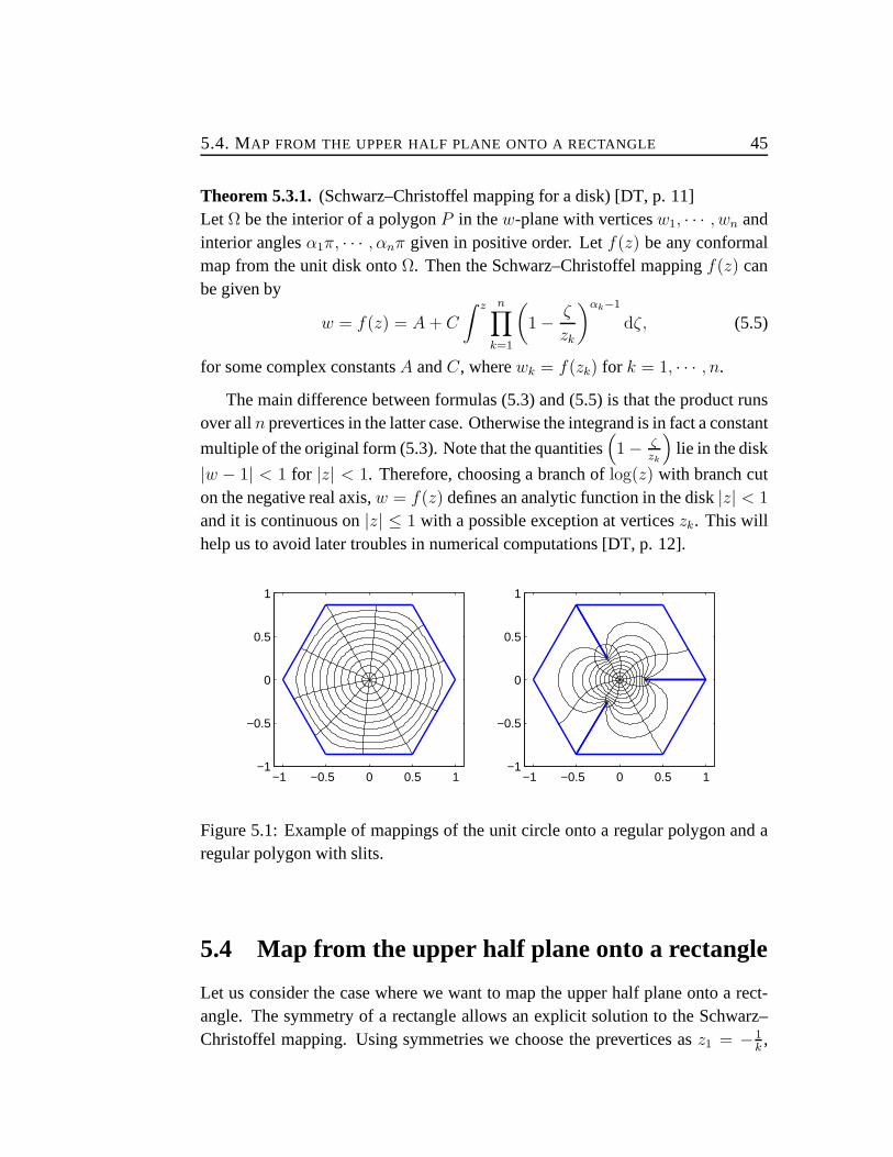
The main difference between formulas (5.3) and (5.5) is thatthe product runsover alln prevertices in the latter case. Otherwise the integrand is in fact a constant

multiple of the original form (5.3). Note that the quantities(

1 − ζzk

)

lie in the disk

|w − 1| < 1 for |z| < 1. Therefore, choosing a branch oflog(z) with branch cuton the negative real axis,w = f(z) defines an analytic function in the disk|z| < 1

and it is continuous on|z| ≤ 1 with a possible exception at verticeszk. This willhelp us to avoid later troubles in numerical computations [DT, p. 12].

−1 −0.5 0 0.5 1−1

−0.5

0

0.5

1

−1 −0.5 0 0.5 1−1

−0.5

0

0.5

1

Figure 5.1: Example of mappings of the unit circle onto a regular polygon and aregular polygon with slits.

5.4 Map from the upper half plane onto a rectangle

Let us consider the case where we want to map the upper half plane onto a rect-angle. The symmetry of a rectangle allows an explicit solution to the Schwarz–Christoffel mapping. Using symmetries we choose the prevertices asz1 = − 1

k,


z2 = −1, z3 = 1 andz4 = 1k, wherek, the elliptic modulus, present the degree of

freedom in the prevertices. The Schwarz–Christoffel mapping can be expressedby an elliptic integral of the first kind

f(z) = A+ C1

∫ z 4∏

j=1

dζ√ζ − zj

= C1

∫ z

0

dζ√

(ζ2 − k−2)(ζ2 − 1)

= k2C1

∫ z

0

dζ√

(k2ζ2 − 1)(ζ2 − 1)

= C

∫ z

0

dζ√

(1 − k2ζ2)(1 − ζ2)

= C

∫ sin φ

0

dθ√

1 − k2 sin2 θ

= CF (k, z).

By rotating, translating, and scaling the rectangle we get thatw3 = f(z3) =

F (k, 1), which is a complete elliptic integral of the first kind. Furthermore thenormalization ensures that the constantC equals1. By denotingw3 = K andcomputingw4 = f(z4) = f

(1k

), we have

w4 =

∫ 1

k

0

dζ√

(1 − k2ζ2)(1 − ζ2)

0<k<1=

∫ 1

0

dζ√

(1 − k2ζ2)(1 − ζ2)︸︷︷︸

= K(k)

+

∫ 1

k

1

dζ√

(1 − k2ζ2)(1 − ζ2).

To transform the latter integral∫ 1

k

1

dζ√

(1 − k2ζ2)(1 − ζ2), (5.6)

we make the change of variable as follows

η =

√

ζ2 − 1

k′ζ⇐⇒ ζ =

1√

1 − k′2η2.

Hence

dζ =k′2η dη

(1 − k′2η2)3

2

,

5.4. MAP FROM THE UPPER HALF PLANE ONTO A RECTANGLE 47

wherek′ is the complementary elliptic modulus given byk′ =√

1 − k2. Thennew integral boundaries are

ζ = 1 ⇒ η = 0,

ζ =1

k⇒ η = 1.

The integrand (5.6) can be written as a product of the following two factors

1√

1 − ζ2=

1√

1 − 11−k′2η2

=1

√

− k′2η2

1−k′2η2

=i√

1 − k′2η2

k′η,

1√

1 − k2ζ2=

1√

1 − k2 11−k′2η2

=1

√1−k′2η2−(1−k′2)

1−k′2η2

=

√

1 − k′2η2

k′√

1 − η2.

So the integral (5.6) can be written by

∫ 1

k

1

dζ√

(1 − k2ζ2)(1 − ζ2)=

∫ 1

0

√

1 − k′2η2

k′√

1 − η2

i√

1 − k′2η2

k′η

k′2η

(1 − k′2η2)3

2

dη

= i

∫ 1

0

dη√

(1 − k′2η2)(1 − η2)

= iK(k′)

= iK ′(k).

That is, the preverticez4 = 1k

is mapped onto the pointw4 = K(k) + iK ′(k). Bythe symmetry of a rectangle, the preverticesz1 = − 1

kandz2 = −1 are mapped

onto pointsw1 = −K(k) + iK ′(k) andw2 = −K(k), respectively. This alsoimplies that the modulus of a quadrilateral can be given by

M(Q;w1, w2, w3, w4) =K ′(k)

2K(k).


Figure 5.2 illustrates the correspondence of vertices under a conformal map of apolygonal domain onto a rectangle.

©

♥

Möbius

− 1k−1 1 1

k

© ♥ −K K

K + iK ′−K + iK ′

©

♥

SC-mapping F (k, z)

Figure 5.2: Illustration, how to conformally map a polygonal domain onto a rect-angle.

Chapter 6

Finite element methods

There are two popular ways to approximate the solution of a partial differentialequation (PDE), namely the finite difference method (FDM) and the finite elementmethod (FEM). The former dominated the early development ofnumerical anal-ysis. In finite difference methods an approximation to the solution is obtained byfinite mesh of points where derivatives of the differential equation are replaced byappropriate difference quotients. This procedure reducesthe problem to a finitelinear system [LT, p. 43].

Finite element methods were introduced in1960s and are probably the mostused method in engineering. Finite element methods are based on a variationalform of partial differential equations and involve an approximation of the exactsolution by piecewise polynomial functions. This makes finite element methodsto be more easily adapted to the underlying domain than finitedifference methods.For symmetric positive definite elliptic equations such as Laplace equation, theproblem reduces to a finite linear system with a positive definite matrix [LT, p.51].

The rest of the chapter is devoted to the analysis of finite element methodssince available numerical packages are revolved around it,even though finite dif-ference methods could be used as well.

49

50 6. FINITE ELEMENT METHODS

6.1 Variational formulation of Laplace equation

Let us consider the following Dirichlet boundary value problem of Laplace equa-tion

−∆u = f, in Ω,

u = 0, on∂Ω,(6.1)

By assumingu ∈ C2(Ω), we multiply the above equation by a test functionψ ∈C1

0 (Ω) and integrate over the domainΩ. Then by applying Green’s formula∫

Ω

ψ∆ϕ dx dy =

∫

∂Ω

ψ∂ϕ

∂nds−

∫

Ω

∇ψ · ∇ϕ dx dy

we have for the left-hand side∫

Ω

∆uψ dx dy =

∫

∂Ω

ψ∇u∂n

ds−∫

Ω

∇u · ∇ψ dx dy, ∀ψ ∈ C10 (Ω).

Recall thatψ ∈ C10(Ω) and we get

−∫

Ω

∆uψ dx dy =

∫

Ω

∇u · ∇ψ dx dy =

∫

Ω

fψ dx dy, ∀ψ ∈ C10(Ω)

Denote

a(u, ψ) =

∫

Ω

∇u · ∇ψ dx dy,

(f, ψ) =

∫

Ω

fψ dx dy.

SinceC10 is dense inH1

0 , it follows

a(u, ψ) = (f, ψ), ∀ψ ∈ H10 (Ω). (6.2)

The variational problem corresponding to (6.1) is to findu ∈ H10 (Ω) such that

(6.2) holds and such a solutionu is called aweakor avariational solutionof (6.1).Thus aclassicalsolution of (6.1) is also a weak solution. On the other hand, byassuming thatu ∈ H1

0(Ω) andu ∈ C2(Ω), then it follows thatu is a classicalsolution of (6.1) as well.

For a non-zero Dirichlet boundary value problem we have to define a conceptof a trace operator. By a trace we means a way to assigning boundary valuesalong∂Ω to a functionu ∈ H1(Ω), assuming that∂Ω ∈ C1. Obviously if u ∈C1(Ω) thenu has boundary values in a natural sense. The problem arises whenu ∈ H1(Ω) and therefore it is not generally continuous, and even worseit is onlydefined almost everywhere inΩ [Eva, pp 257–259].

6.1. VARIATIONAL FORMULATION OF LAPLACE EQUATION 51

Theorem 6.1.1.(Trace theorem) [Eva, p. 258]AssumeΩ is bounded and∂Ω ∈ C1. Then there exists a trace operator

Tr : H1 → L2(∂Ω)

such that‖Tr(u)‖L2(∂Ω) ≤ C‖u‖H1(Ω), ∀u ∈ H1(Ω),

where the constantC depends only onΩ. We callTr(u) the trace ofu on∂Ω.

Now consider a non-zero Dirichlet boundary value problem

−∆u = f, in Ω,

u = g, on∂Ω.(6.3)

Suppose that∂Ω ∈ C1 andu ∈ H1(Ω) is a weak solution of (6.3). This impliesthatu = g on∂Ω in the trace sense which means thatg has to be the trace of someH1 function, sayh. Thenu = u − h belongs toH1

0 (Ω), and it is a weak solutionof the boundary value problem

−∆u = f , in Ω,

u = 0, on∂Ω,

wheref = f + ∆h.For the Neumann boundary value problem of Laplace equation

−∆u = f, in Ω,

∂u

∂n= 0, on∂Ω,

(6.4)

we use the same argument as above to obtain the variational formulation cor-responding to (6.4). Because∂u

∂n= 0, we takeψ ∈ H1(Ω) instead of taking

ψ ∈ H10 (Ω). Therefore we have

a(u, ψ) = (f, ψ), ∀ψ ∈ H1(Ω). (6.5)

The variational problem corresponding to (6.4) is to findu ∈ H1(Ω) such that(6.5) holds.

Finally considering the Laplace equation with the Dirichlet–Neumann bound-ary value problem (4.1)

∆u = 0, in Ω,

u = 0, onγ2,

u = 1, onγ4,

∂u

∂n= 0, onγ1 ∪ γ3.


By above arguments we obtain the following variational formulation:

a(u, ψ) = 0, ∀ψ ∈ H10 (Ω).

The above discussions can be stated in more general manner. See [Eva, pp. 293–297] for more details.

6.2 Finite element mesh

The first task in finite element methods is to define a finite element to work with.We have to give some properties that the finite element have tosatisfy in order tobe useful. After defining a finite element, we need a way to connect finite elementstogether which requires more from the elements.

Definition 6.2.1. (Finite element) [SSD, p. 1]A finite elementis a triadK = (K,P,Σ), where

• K is a domain inR2. It can be either a triangle or a quadrilateral.

• P is a space of polynomials on K of the dimensiondim(P ) = NP .

• Σ = L1, L2, · · · , LNP is a set of linear forms

Li : P → R, i = 1, 2, · · · , NP .

The elements ofΣ are calleddegrees of freedom.

Definition 6.2.2. (Unisolvency of finite element) [SSD, p. 2]The finite elementK = (K,P,Σ) is said to beunisolventif for every functionp ∈ P it holds that

L1(g) = L2(g) = · · · = LNP(g) = 0 ⇒ g = 0.

In other words, every vector of numbers

L(g) = (L1(g), L2(g), · · · , LNP(g))T ∈ R

NP

identifies a unique polynomialg in the spaceP .

Unisolvency is a way to express a compatibility of the set of degrees of free-dom inΣ with the polynomial spaceP .

6.2. FINITE ELEMENT MESH 53

Theorem 6.2.3.(Characterization of unisolvency) [SSD, p. 3]Consider a finite elementK = (K,P,Σ), dim(P ) = NP . The finite elementK isunisolvent if and only if there exists a unique basisB = θ1, θ2, · · · , θNP

⊂ P

satisfying a followingδ–property

Li(θj) = δij , 1 ≤ i, j ≤ NP ,

whereδij is the Kronecker delta defined by

δij =

1, i = j,

0, i 6= j.

Proof:”⇒” Let g1, g2, · · · , gNP

⊂ P an arbitrary basis and we express sought func-tionsθj , j = 1, · · · , NP , by

θj =

NP∑

k=1

akjgk.

For theδ-property, we require that

Li(θj) = Li

(NP∑

k=1

akjgk

)

=

NP∑

k=1

akjLi(gk) = δij , 1 ≤ i, j ≤ NP .

This yields a linear system ofNP variables and can be given by matrix equationas

LA = I,

where column of matrixA contains the coefficients of the functionsθ1, θ2, · · · , θNP.

Since the elementK is unisolvent it follows thatL is invertible and thatθ1, θ2, · · · , θNP

are uniquely determined. Next we show thatθ1, θ2, · · · , θNPare linearly indepen-

dent, that is

NP∑

k=1

βkθk = 0 ⇒ β1 = β2 = · · · = βNP= 0.

By evaluating the functionsLi with the above linear combinations we get

0 = Li

(NP∑

k=1

βkθk

)

=

NP∑

k=1

βkLi(θk) = βi, ∀ i = 1, 2, · · · , NP .


”⇐” Let B = θ1, θ2, · · · , θNP a basis of the spaceP satisfying theδ-property.

Then every functionp ∈ P can be expressed by

p =

NP∑

k=1

βkθk.

Assuming thatL1(g) = L2(g) = · · · = LNP

(g) = 0,

immediately we have

0 = Li(g) = Li

(NP∑

k=1

βkθk

)

= βi, ∀ i = 1, 2, · · · , NP .

Hence it follows thatg = 0 and the finite elementK is unisolvent [SSD, pp. 3–4].

The proof of Theorem 6.2.3 gives us a convenient way to check the unisol-vency of the finite elementK in form of invertibility of the matrixL. Here wehave discussed about the unisolvent of a single finite element K. Next we willaddress the compatibility of finite elements of function spaces which are used foran approximation. We called this compatibility byconformityof finite elementsto function spaces.

Suppose that a domainΩ is bounded with the boundary∂Ω ∈ C1, where theunderlying partial differential equation is considered. ThenΩ is approximated bya computational domainΩh whose boundary is a piecewise polynomial.

Definition 6.2.4. (Finite element mesh) [SSD, p. 7]A finite element meshTh,p = K1, K2, · · · , KM over a domainΩh with a piece-wise polynomial boundary is a geometrical partition ofΩh into a finite number ofnon-overlapping open polygonalKi such that

Ωh =M⋃

i=1

Ki,

and eachKi, 1 ≤ i ≤M , is equipped with a polynomial orderp(Ki) = pi ≥ 1.

A finite element mesh is calledregular if for any two elementsKi andKj,i 6= j, only one of the following statements hold

• Ki andKj are disjoint,

6.2. FINITE ELEMENT MESH 55

• Ki andKj have only one common vertex,

• Ki andKj have only one common edge.

By a regular mesh we avoidhanging nodeswhich complicate the discretizationprocess. A mesh with hanging nodes is calledirregular.

Regular mesh Irregular mesh

Figure 6.1: Finite element meshes, on the left a regular and on the right an irreg-ular mesh with one hanging node.

Definition 6.2.5. (Interpolant) [SSD, p. 9]Given a unisolvent finite element(K,P,Σ), letB = θ1, · · · , θNP

be the uniquebasis ofP satisfying theδ-property. Letv ∈ V , whereP ⊂ V , be a function forwhich allL1, · · · , LNP

are defined. Then we define a localinterpolantby

IK(v) =

NP∑

i=1

Li(v)θi.

The global interpolantI over a finite meshTh,p is defined by means of localinterpolants by

I(v)|Ki≡ IKi

(v), i = 1, · · · ,M.

Definition 6.2.6. (Conformity of finite elements) [SSD, p.10]LetTh,p be a finite element mesh consistingM unisolvent finite elements(Ki, Pi,Σi),i = 1, 2, · · · ,M . Let V (Ωh) beH1 and letIKi

: V (Ki) → Pi be the local finiteelement interpolation operator. We sayTh,p is conforming to the spaceH1 if foreach common edge of elementsKi andKj ,Ki, Kj ∈ Th,p the trace ofv|Ki

equalsto the trace ofv|Kj

on the edge.


In higher order finite elements methods we have lots of overlapping infor-mations on each element and an effective management is needed. Therefore theusage of the reference elementKref is encouraged. The task is to find areferencemappingFKi

: Kref → Ki that is smooth and bijective. The polynomial spacewith the reference mapFKi

is used for define the function spaceVh,p(Ωh), wherethe finite element solution is sought [SSD, pp. 16–17].

6.3 Shape functions

Shape functions are functions used for approximating the solution to partial dif-ferential equations. There are numerous ways to select shape functions but wewill be usingLegendre’s polynomials, since they possess many useful properties.Though there are many ways to define Legendre’s polynomials,the definitionthrough a recursive formula is the most useful way to implement the higher ordershape functions.

Definition 6.3.1. (Legendre’s polynomial) [Leb, p. 46]Legendre’s polynomialsof degreen can be defined recursively by

(n+ 1)Pn+1(x) − (2n+ 1)xPn(x) + nPn−1(x) = 0, .

whereP0(x) = 1 andP1(x) = x.

First few Legendre’s polynomials are

P0(x) = 1,

P1(x) = x,

P2(x) =3

2x2 − 1

2,

P3(x) =5

2x3 − 3

2x.

The derivatives of Legendre’s polynomials can also be givenby a recursive for-mula as follow

(1 − x2)P ′n(x) = nPn−1(x) − nxPn(x), n ≥ 1.

By manipulating the derivatives further we have

[(1 − x2)P ′

n(x)]′

+ n(n+ 1)Pn(x) = 0, n ≥ 0. (6.6)

6.3. SHAPE FUNCTIONS 57

One of the most important properties of Legendre’s polynomials is the orthog-onality in the interval[−1, 1]. This can be shown from the differential equation(6.6). First we multiply thenth differential equation byPm(x) and subtract it fromthemth differential equation multiplied byPn(x), which leads to

0 =[(1 − x2)P ′

m(x)]′Pn(x) +m(m+ 1)Pm(x)Pn(x)

−[(1 − x2)P ′

n(x)]′Pm(x) − n(n+ 1)Pn(x)Pm(x). (6.7)

By the identity[(1 − x2)P ′

m(x)Pn(x)]′

=[(1 − x2)P ′

m(x)]′

+ (1 − x2)P ′m(x)P ′

n(x),

and the symmetry between indicesm andn, we rewrite the equation (6.7) in form[(1 − x2) (P ′

m(x)Pn(x) − P ′n(x)Pm(x))

]′+(m−n)(m+n+1)Pm(x)Pn(x) = 0.

Then by integrating over the interval[−1, 1], the first term vanishes because(1 −x2) vanishes and we have

∫ 1

−1

(m− n)(m+ n+ 1)Pm(x)Pn(x) dx = 0,

which yields the orthogonality of Legendre’s polynomials [Leb, pp. 47–50]. Itcan also be shown that the norm is given by

‖Pn‖2 =

(∫ 1

−1

P 2n(x) dx

)1/2

=

√

2

2n+ 1.

Let us define functionsφj as the integrated Legendre’s polynomials. Then wehave

φ0(ξ) =1 − x

2,

φ1(ξ) =x− 1

2,

φj(ξ) =1

‖Pj−1‖2

∫ ξ

−1

Pj−1(t) dt

=

√

2j − 1

2

∫ ξ

−1

Pj−1(t) dt, j ≥ 2,

and we can rewrite them by mean of Legendre’s polynomials

φj(ξ) =1

√

2(2j − 1)[Pj(ξ) − Pj−2(ξ)] , j ≥ 2.


Note thatφj(−1) = 0, k ≥ 1, and they are orthogonal

∫ 1

−1

dφi(ξ)

dξ

dφj(ξ)

dξdξ = δij , i, j ≥ 2.

The integrated Legendre’s polynomials form a shape function basis to be used infinite elements methods. In particular, they play an essential role in a constructionof a hierarchic basis [SSD, p. 25], [SB, pp. 38–39].

For other definitions and for more details regarding Legendre’s polynomialssee [Leb, Sze].

Definition 6.3.2. (Hierarchic basis) [SB, p. 96]Suppose that the basisBp consist of polynomials of orderp. ThenBp is said to behierarchic if Bp ⊂ Bp+1.

In case of quadrilateral elements, we use[−1, 1] × [−1, 1] as the referenceelement. In order to satisfy the conformity requirements ofthe finite elementmesh, we divide shape functions into three categories:nodal shape functions,side modes, andinternal modes. We follow a presentation of Szabó and Babuška[SB, pp. 98–100] and present the shape functions as follows.

1. Nodal shape functions.Nodal shape functions are defined so that they getvalue one at only one vertex and vanish on the other vertices.There are totalof 4 nodal shape functions and they are defined by

N1(ξ, η) =1

4(1 − ξ)(1 − η),

N2(ξ, η) =1

4(1 + ξ)(1 − η),

N3(ξ, η) =1

4(1 + ξ)(1 + η),

N4(ξ, η) =1

4(1 − ξ)(1 + η).

2. Side Nodes.There are4(p−1) side modes and they associate with only oneedge of the finite element and vanish on the other edges. For side modes we

6.4. HIGHER-ORDER FINITE ELEMENT METHODS 59

have (p ≥ 2)

N1i (ξ, η) =

1

2(1 − η)φi(ξ), i = 2, 3, · · · , p,

N2i (ξ, η) =

1

2(1 + ξ)φi(η), i = 2, 3, · · · , p,

N3i (ξ, η) =

1

2(1 + η)φi(ξ), i = 2, 3, · · · , p,

N4i (ξ, η) =

1

2(1 − ξ)φi(η), i = 2, 3, · · · , p,

where the superscript determines the edge of the finite element which theside mode function associate with.

3. Internal modes. For internal modes we have two different options to choosefrom. Thetrunkspace which has(p−2)(p−3)

2shape functions and they are de-

fined by

Nij(ξ, η) = φi(ξ)φj(η), i, j ≥ 2, 4 ≤ i+ j ≤ p.

On the other hand thefull space has(p− 1)(p− 1) shape functions, whichare defined by

Nij(ξ, η) = φi(ξ)φj(η), i, j = 2, 3, · · · , p.

Note that internal modes vanish on the boundary of the reference element.This is the reason why they are sometimes referred to asbubble functions.

See Appendix A for an illustration of some of the shape functions.

6.4 Higher-order finite element methods

There are three different kinds of higher order finite element methods, namelyh-, p-, andhp-version. Theh-version of finite element methods is consideredas the most popular version. Inh-version the degree of freedom of elements arefixed by fixing the order of the polynomial space and a convergence is obtainedby refining the mesh where errors are large. This can be done bycomputing theestimated error for each element. On the other hand,p-version of the finite elementmethods uses fixed elements and the convergence is obtained by increasing the


degree of elements that is the order of the polynomial space.Lastly thehp-versionsimultaneously refines the mesh and increases the degree of elements. For moredetailed discussion of the error analysis of higher order finite element methods,see series of papers by Gui and Babuška [GB1, GB2, GB3].

Chapter 7

Numerics of the modulus of aquadrilateral

There are two natural approaches to compute the modulus of a quadrilateral.Through the definition of the modulus and use of the conformalmapping fromgiven domain onto a rectangle and methods that will only givethe modulus. Theformer methods give the conformal mappings as well and usually involves solvinga parameter problem for the Schwarz–Christoffel mapping. While the latter givesonly the modulus, which we are interested in. Also the lattermethods usually de-pends on solving the Dirichlet–Neumann boundary value problem for the Laplaceequation.

Methods for numerical computation of the Schwarz–Christoffel mapping dateback to around1960. In 1980 Trefethen [Tre] introduced theside-lengthmethodbased on works by Relly and others. Driscoll and Vavasis [DrVa] proposed in1998 an algorithmCRDT(cross-ratios of the Delaunay triangulation) to overcomecrowding [DT, p. 23]. Recently Banjai [Ban] gave modifications to Trefethen’salgorithm to improve the accuracy of the computation of someelongated domains,which are the main cause of the crowding phenomenon.

Finite element methods can be applied to solve the Dirichlet–Neumann bound-ary value problem for the Laplace equation (4.1). In2004 Samuelsson [BSV]described an AFEM (adaptive finite element method) softwarepackage based onan h-version finite element method. Recently Hakula [HRV] introduced an al-gorithm to anhp-version of finite element method for Mathematica. Both of theabove methods can be applied to compute the modulus of a quadrilateral.

For side-length and CRDT methods a numerical integration isneeded. Usualnumerical integration methods give poor results since the Schwarz–Christoffel in-

61

62 7. NUMERICS OF THE MODULUS OF A QUADRILATERAL

tegral is usually singular at prevertices. To compute the integral, we use aGauss–Jacobiquadrature, which is too lengthy to be described here. See [DT, pp. 28–30]for more details about Gauss–Jacobi quadrature.

The rest of the chapter, we discuss above the methods in more details anddiscuss the crowding phenomenon.

7.1 Side-length

To compute the Schwarz–Christoffel mapping using the side-length method, wemust solve a parameter problem, which is in general non-linear. For Schwarz–Christoffel mappings we have three degrees of freedom. By choosing preverticeszn−2, zn−1 andzn from the boundary of the domain, we are left withn − 3 quan-tities to be determinate by the following system of equations

∣∣∣∣∣

∫ zj+1

zj

f ′(ζ) dζ

∣∣∣∣∣

∣∣∣∣

∫ z2

z1

f ′(ζ) dζ

∣∣∣∣

=|wj+1 − wj||w2 − w1|

, j = 2, 3, · · · , n− 2,

∫ zJ+1

zJ−1

f ′(ζ) dζ

∣∣∣∣

∫ z2

z1

f ′(ζ) dζ

∣∣∣∣

=wJ+1 − wJ−1

|w2 − w1|, if wJ = ∞ for J < n,

(7.1)

wheref ′(z) can be obtained from (5.3). In case of the unit circle, using the for-mula (5.5) instead of (5.3) is a better option. In addition, we must require that notwo infinite vertices are adjacent. This can be achieved by introducing a degener-ated vertex with the interior angleπ on the straight line between infinite adjacentvertices [DT, pp. 23-25].

For details how this can be done in case of the unit circle see [DT, pp. 25-27]or the original paper by Trefethen [Tre].

7.2 CRDT

The CRDT algorithm has several phases in order to construct the Schwarz–Christoffelmapping. First we have to triangulate the given simple polygonP by using one

7.2. CRDT 63

kind of Delaunay triangulation process. Then we split the edges using edge split-ting algorithm. Finally we use cross-ratios and solve the emerging parameterproblem to determine the prevertices ofP .

The Delaunay triangulation

A triangulation ofP is a partition ofP into non-degenerate triangles, whose ver-tices are vertices ofP . If triangles intersect, they must intersect on a vertex oron an entire edge. It can be proved by induction, that a triangulation ofP con-sists exactly ofn − 2 triangles andn − 3 diagonals, which are edges of trianglesthat are not also the edges ofP . Furthermore, ifd is a diagonal, letQ(d) be thequadrilateral, the union of the two triangles on either sideof d. Remark that thetriangulation ofP is not unique.

Splitting edges

To avoid quadrilaterals that are long and narrow, we split the edges so that thequadrilaterals in the Delaunay triangulation are well conditioned. By ”well con-ditioned” we mean that the prevertices of the quadrilaterals are not too crowded.

The splitting procedure has two phases. In the first phase, weare lookingfor verticesw with an interior angle less than or equal toπ

4. For every such a

preverticesw, find a largest isosceles triangleT that can be formed byw with itsadjacent edges such thatT is contained inP . Next we introduced new vertices atmidpoints of the two sides ofT that are the edges adjacent tow and we call theseadjacent edges tow asprotected. That is, we do not allow them to be split duringthe second phase. LetP ′ denote the polygon obtained after the first phase of thesplitting procedure.

On the second phase we iteratively split the polygonP ′ into partitions. Letebe an unprotected edge of some polygon during the splitting procedure. Letl(e)be its length and letd(e) be the smallest distance frome to any vertex except theendpoints ofe. The distance is measured along the shortest piecewise linear paththat remains inside the polygon. The edgee is said to be ill separated if

d(e) <l(e)

3√

2.

Then the ill conditioned edges are split into three equal parts. It can be proved thatthe second phase of the splitting procedure will end in a finite number of steps.


Cross-ratios

Like side-length method, CRDT also haven− 3 variable to be determined. Thesevariables are determined using cross ratios of prevertices. Let d1, · · · , dn−3 bediagonals and letQ1 = Q(d1), · · · , Qn−3 be quadrilaterals of the Delaunay tri-angulation ofP . Denote the vertices ofQi by wκ(i,1), wκ(i,2), wκ(i,3), wκ(i,4) foreachi = 1, · · · , n − 3, whereκ(i, 1), κ(i, 2), κ(i, 3), κ(i, 4) is distinct indices in1, · · · , n.

For a given list of preverticesz1, · · · , zn, we compute variablesσi, which aredefined by

σi = ln(−(zκ(i,1), zκ(i,2), zκ(i,3), zκ(i,4))), i = 1, · · · , n− 3. (7.2)

Notice that there aren real variables and onlyn− 3 real constraints. By choosinga Delaunay triangularT0 in the way that its prevertices are arbitrarily placed onthe unit circle in a manner of preserving the order. Then there exists a unique wayto determine the remainingn − 3 zi’s on the unit circle satisfying (7.2). It turnsout that the choice forT0 does not matter, we will end up with the same polygon,up to a similarity transformation [DrVa].

7.3 Adaptive finite element methods

AFEM

In order thea posterioriestimate to work well, AFEM triangulate the domain tohave certain properties. For example, the lower bound of thesmallest angle of thetriangulation must be fixed. The refined elements must have these properties aswell. For detailed properties and algorithms, see [BSV].

hp-FEM

In hp-FEM, the mesh of a polygonal domain is generated in two phasealgorithm:

1. Generate a minimal mesh where the vertices are isolated with a fixed num-ber of triangle depending on the interior angleα:

• α ≤ π2: one triangle,

• π2≤ α < π: two triangles,

• α ≥ π: three triangles.

7.4. HEIKKALA –VAMANAMURTHY –VUORINEN ITERATION 65

2. Every triangle attached to vertices is replaced by refinedtriangles where theedges adjacent to the vertex are split as specified by the scaling factorr.This process is repeated recursively until the the nesting levelν is reached[HRV].

The refined mesh is referred as(r, ν)-mesh. An example is shown in Figure 7.1.The actual numerical computation for the solution of (4.1) is done as described inChapter 6.

Figure 7.1: A quadrilateralQ(0, 1, 3

10+ 3

10i, i)

with the initial mesh and the(0.4, 2)-mesh on the left- and right-hand side, respectively.

7.4 Heikkala–Vamanamurthy–Vuorinen iteration

Heikkala, Vamanamurthy, and Vuorinen [HVV] proposed an iteration which canbe used for compute the modulus of a quadrilateral. The iteration consists ofevaluations of hypergeometric functions, beta functions,and elliptic integrals.

Definition 7.4.1. (Gaussian hypergeometric function) [HVV, p. 1]Given complex numbersa, b,andc with c 6= 0,−1,−2, · · · , theGaussian hyper-geometric functionis the analytic continuation to the slit planeC\[1,∞) of theseries

F (a, b; c; z) = 2F1(a, b; c; z) =

∞∑

n=0

(a, n)(b, n)

(c, n)

zn

n!, |z| < 1.


Here(a, 0) = 1 for a 6= 0, and(a, n) is theshifted factorial functionor theAppellsymbol

(a, n) = a(a + 1)(a+ 2) · · · (a+ n− 1)

for n ∈ N.

Definition 7.4.2. (Beta function) [HVV, p. 10]Let Re(x) > 0 andRe(y) > 0. Then thebeta functionis defined by

B(x, y) =

∫ 1

0

tx−1(1 − t)y−1 dt.

Theorem 7.4.3.Let 0 < a, b < 1, maxa + b, 1 ≤ c ≤ 1 + mina, b. SupposethatQ is a quadrilateral in the upper half plane with vertices0, 1, A, andB, theinterior angles at which are, respectively,bπ, (c− b)π, (1− a)π, and(1+ a− c)π.Then the modulus ofQ is given by

M(Q; 0, 1, A,B) =K ′(k)

K(k),

where the elliptic modulusk satisfies the equation

A− 1 =Lk′2(c−a−b)F (c− a, c− b; c + 1 − a− b; k′2)

F (a, b; c; r2),

and

L =B(c− b, 1 − a)

B(b, c− b)e(b+1−c)iπ.

Proof: See [HVV, p. 7].Note that the quadrilateralQ in Theorem 7.4.3 is convex. There is a slight

chance that the iteration works for a non-convex quadrilateral as well.

7.5 Crowding

The biggest obstacle for numerical methods of conformal mappings is a so calledcrowding. Crowding is a form of ill-conditioning which is present in virtually allnumerical methods of conformal mappings. Crowding occurs when two prever-tices are too close to each other. It might be numerically impossible to distinguishthe two prevertices from each other, because of the limited accuracy of the numer-ical floating point arithmetics [DT, pp. 20–21].

7.5. CROWDING 67

The situation can be illustrated by a long and thin rectangles. Consider a mapf(z) that maps a quadrilateralQ(Ω, 1 + iM, iM, 0, 1) onto the unit diskD suchthatf(1 + iM) = −f(0) andf(iM) = −f(1). Then the minimal distance of theimage pointsf(1+iM), f(iM), f(0), andf(1) is less than3.4 ·10−16 forM = 1

24

[HRV], [Pap, pp. 131–132].

Chapter 8

Numerical results

In this chapter we consider quadrilaterals and compute its modulus by differentnumerical tools introduced in Chapter 7. Then the results are compared to thereference value as well as with each other.

8.1 Symmetric quadrilateral

In this section we usehp-version of finite element methods [HRV] to run series oftests on a symmetric quadrilateral with vertices0, 1, 0.3 + 0.3i, i. See Figure 7.1for an illustration. By Theorem 4.2.2 we know that the modulus is exactly one.

8.1.1 Scaling factor

Let us consider the scaling factor. We use the(r, 12)-meshes, wherer ∈ [0.1, 0.5]

with polynomial degree of4, 6, · · · , 18. Using different polynomial degrees weidentify the effect of the scaling factor. The result of the logarithmic error is shownin Figure 8.1. The result shows that for a fixed nesting levelν and different polyno-mial degree there exists a optimal scaling factor. Generally the higher polynomialdegree is, the smaller the scaling factor should be chosen. We emphasize that theresult is only valid for this particular quadrilateral. Forother configurations theoptimal scaling factor may vary. There might also be an analytical formula forrelations between the polynomial degree and the optimal scaling factor.

69

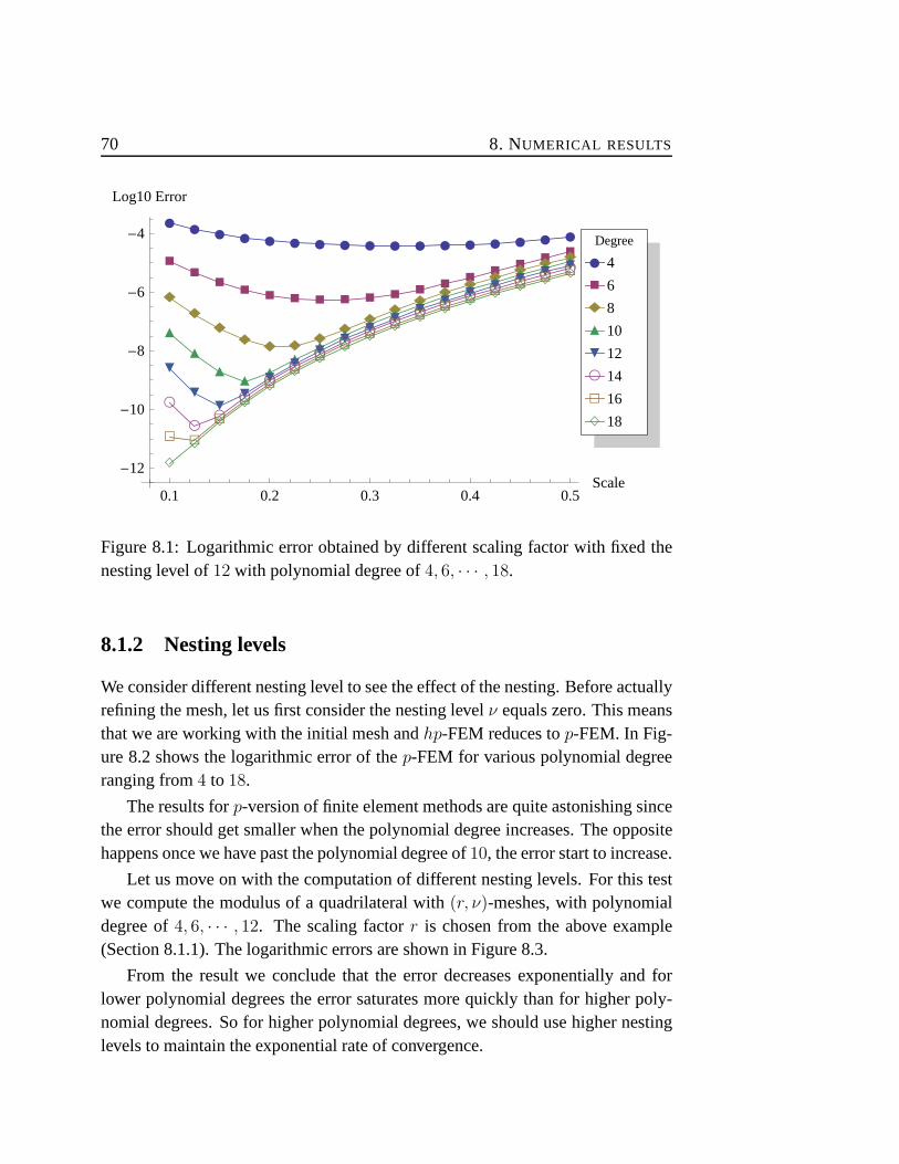
70 8. NUMERICAL RESULTS

æææ æ æ æ æ æ æ æ æ æ æ æ æ æ æ

ààààà à à à à à

ààààààà

ì

ìììì ì

ììììììììììì

ò

ò

òòòòòòòòòòòòòòò

ô

ôôô

ô

ôôôôôôôôôôôô

ç

çç

ç

ç

çççççççççççç

á á

á

á

á

áááááááááááá

í

í

í

í

í

íííííííííííí

0.1 0.2 0.3 0.4 0.5Scale

-12

-10

-8

-6

-4

Log10 Error

í 18

á 16

ç 14

ô 12

ò 10

ì 8

à 6

æ 4

Degree

Figure 8.1: Logarithmic error obtained by different scaling factor with fixed thenesting level of12 with polynomial degree of4, 6, · · · , 18.

8.1.2 Nesting levels

We consider different nesting level to see the effect of the nesting. Before actuallyrefining the mesh, let us first consider the nesting levelν equals zero. This meansthat we are working with the initial mesh andhp-FEM reduces top-FEM. In Fig-ure 8.2 shows the logarithmic error of thep-FEM for various polynomial degreeranging from4 to 18.

The results forp-version of finite element methods are quite astonishing sincethe error should get smaller when the polynomial degree increases. The oppositehappens once we have past the polynomial degree of10, the error start to increase.

Let us move on with the computation of different nesting levels. For this testwe compute the modulus of a quadrilateral with(r, ν)-meshes, with polynomialdegree of4, 6, · · · , 12. The scaling factorr is chosen from the above example(Section 8.1.1). The logarithmic errors are shown in Figure8.3.

From the result we conclude that the error decreases exponentially and forlower polynomial degrees the error saturates more quickly than for higher poly-nomial degrees. So for higher polynomial degrees, we shoulduse higher nestinglevels to maintain the exponential rate of convergence.

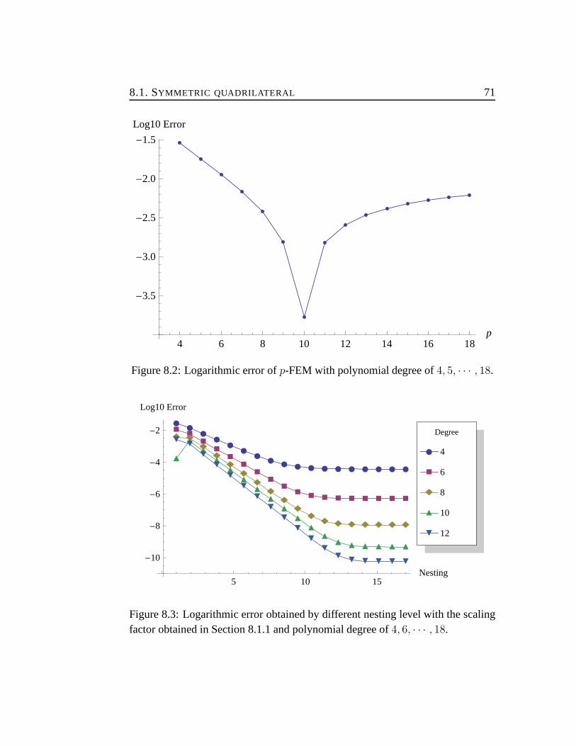
8.1. SYMMETRIC QUADRILATERAL 71

4 6 8 10 12 14 16 18p

-3.5

-3.0

-2.5

-2.0

-1.5

Log10 Error

Figure 8.2: Logarithmic error ofp-FEM with polynomial degree of4, 5, · · · , 18.

æææææææææ æ æ æ æ æ æ æ æ æ

àà

à

à

à

à

ààààà à à à à à à à

ì ììììììììììì ì ì ì ì ì ì

ò

ò

ò

ò

ò

ò

ò

ò

ò

ò

òòò ò ò ò ò ò

ôô

ô

ô

ô

ô

ô

ô

ô

ô

ô

ôôô ô ô ô ô

5 10 15Nesting

-10

-8

-6

-4

-2

Log10 Error

ô 12

ò 10

ì 8

à 6

æ 4

Degree

Figure 8.3: Logarithmic error obtained by different nesting level with the scalingfactor obtained in Section 8.1.1 and polynomial degree of4, 6, · · · , 18.


8.1.3 Refining vertices

In [BS] basic principles and properties are given top- andhp-versions of finiteelement methods. One of the properties says that most of the error comes fromthe so called singularity component which is the vertex witha largest interiorangle. In this test we use three different kind of mesh to verify the result. We use(0.15, 12)-meshes and refine the meshes

1. to vertices with interior angles0 < α ≤ π2

(regular vertices),

2. to the singular vertex only,

3. to all vertices.

The polynomial degree is varied from4 to 18. Results of the logarithmic errorsare shown in Figure 8.4.

æ æ æ æ æ æ æ æ æ æ æ æ æ æ æ

à

à

à

à

à

à

à

àà à à à à à à

ì

ì

ì

ì

ììììì ì ì ì ì ì ì

4 6 8 10 12 14 16 18p

-10

-8

-6

-4

-2

0

Log10 Error

ì All

à Singular

æ Regular

Refinement

Figure 8.4: Logarithmic errors of computations of modulus by different meshrefinements on vertices. Notice that the error of refining allvertices and refiningthe singular vertex alone are indistinguishable.

The result suggests that the we cannot get more than3 correct digits for thisexample by refining only the regular vertices. While refiningonly the singularvertex, we may obtain11 correct digits at most. The result of refinement of allthe vertices does not give any significant improvement over the case where werefine only the singular vertex. It should be notice that refining all vertices, the

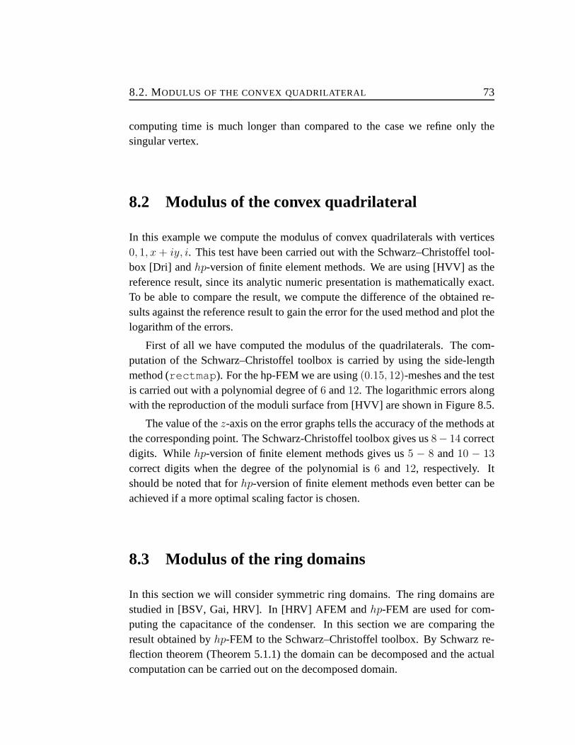
8.2. MODULUS OF THE CONVEX QUADRILATERAL 73

computing time is much longer than compared to the case we refine only thesingular vertex.

8.2 Modulus of the convex quadrilateral

In this example we compute the modulus of convex quadrilaterals with vertices0, 1, x+ iy, i. This test have been carried out with the Schwarz–Christoffel tool-box [Dri] andhp-version of finite element methods. We are using [HVV] as thereference result, since its analytic numeric presentationis mathematically exact.To be able to compare the result, we compute the difference ofthe obtained re-sults against the reference result to gain the error for the used method and plot thelogarithm of the errors.

First of all we have computed the modulus of the quadrilaterals. The com-putation of the Schwarz–Christoffel toolbox is carried by using the side-lengthmethod (rectmap ). For the hp-FEM we are using(0.15, 12)-meshes and the testis carried out with a polynomial degree of6 and12. The logarithmic errors alongwith the reproduction of the moduli surface from [HVV] are shown in Figure 8.5.

The value of thez-axis on the error graphs tells the accuracy of the methods atthe corresponding point. The Schwarz-Christoffel toolboxgives us8− 14 correctdigits. Whilehp-version of finite element methods gives us5 − 8 and10 − 13

correct digits when the degree of the polynomial is6 and 12, respectively. Itshould be noted that forhp-version of finite element methods even better can beachieved if a more optimal scaling factor is chosen.

8.3 Modulus of the ring domains

In this section we will consider symmetric ring domains. Thering domains arestudied in [BSV, Gai, HRV]. In [HRV] AFEM andhp-FEM are used for com-puting the capacitance of the condenser. In this section we are comparing theresult obtained byhp-FEM to the Schwarz–Christoffel toolbox. By Schwarz re-flection theorem (Theorem 5.1.1) the domain can be decomposed and the actualcomputation can be carried out on the decomposed domain.


1

2

3

4

y

1

2

3

4

x

0.81.01.21.4

Mod

1

2

3

4

y1

2

3

4

x

-14

-12

-10

-8

Error

1

2

3

4

y1

2

3

4

x

-10

-8

-6

Error

1

2

3

4

y

1

2

3

4

x

-14

-12

-10

Error

Figure 8.5: On top we have the reproduction of the modulus of the quadrilateralwith vertices0, 1, x+ iy, i from [HVV] and the logarithmic error of the Schwarz–Christoffel toolbox. On bottom we have logarithmic errors of the hp-FEM with(0.15, 12)-meshes and the polynomial degree of6 and12 respectively.

Square in a square

We compute the modulus of the ring domainΩ = Ω1\Ω2, whereΩ1 = [−1, 1] ×[−1, 1] andΩ2 = [−a, a] × [−a, a], 0 < a < 1. For the computation the domainis decomposed into8 quadrilaterals, see Figure 8.6. It can be proved that themodulus of the quadrilateral is doubled if the reflection boundary is Neumannboundary. This implies that the modulus of the original domain equals to8 timesthe modulus of the decomposed quadrilateral.

The computation is carried out by the Schwarz–Christoffel toolbox andhp-FEM. In this case we computed the modulus of the decomposed quadrilateral withthe side-length method (rectmap ) and CRDT (crrectmap ). Forhp-FEM wehave used(0.15, 12)-meshes with polynomial degrees of6, 12, and18. Like inprevious examples, the results are compared to the values obtained from HVV

8.3. MODULUS OF THE RING DOMAINS 75

a

(0, 0) (1, 0)

(a, 1 − a)(0, 1 − a)

Figure 8.6: The domain of interest is on the left-hand side and on the right-handside we have one of the quadrilateral decomposed from the original domain.

iteration. The errors are listed in Table 8.1 along with the modulus obtained byHVV iteration.

Table 8.1: Table for the exact value of the modulus and the error for differentmethods in a square in a square. The parameterp refers to polynomial degree ofhp-FEM. Reference values are obtained by HVV–iteration.

a rectmap crrectmap p = 6 p = 12 p = 18 Reference0.1 5.2 · 10−9 5.3 · 10−7 1.0 · 10−4 7.0 · 10−8 8.1 · 10−11 2.817122196

0.2 8.4 · 10−13 4.1 · 10−8 3.4 · 10−6 2.0 · 10−10 1.6 · 10−14 1.934943792

0.3 1.1 · 10−13 6.3 · 10−10 3.4 · 10−7 4.2 · 10−12 3.3 · 10−15 1.420245745

0.4 3.8 · 10−11 5.7 · 10−12 1.1 · 10−7 2.1 · 10−12 1.8 · 10−15 1.057986726

0.5 2.7 · 10−9 2.4 · 10−11 8.9 · 10−8 1.9 · 10−12 1.2 · 10−15 0.781700961

0.6 7.1 · 10−9 7.2 · 10−12 5.1 · 10−8 1.0 · 10−12 1.1 · 10−16 0.561999833

0.7 3.5 · 10−9 1.6 · 10−9 8.8 · 10−8 9.1 · 10−13 3.8 · 10−15 0.382746154

0.8 1.1 · 10−9 5.2 · 10−10 7.0 · 10−7 1.2 · 10−10 2.6 · 10−14 0.233679562

0.9 2.9 · 10−10 7.4 · 10−10 9.9 · 10−6 2.2 · 10−8 8.8 · 10−11 0.107766002

Since the quadrilaterals are not elongated the CRDT does notstand out fromthe side-length method. For some cases CRDT perform even worse than side-length method and vice versa. In case of hp-FEM we get2−3 more correct digits


by increasing the polynomial degree by6. For0.3 < a < 0.7, hp-FEM with the(0.15, 12)-mesh and polynomial degrees of9− 11 gives the same performance asthe Schwarz–Christoffel toolbox.

We have only emphasized how to improve the performance ofhp-version offinite element methods. In the Schwarz–Christoffel toolboxwe can change thetolerance rate to obtain much better result. In Table 8.2 we have the result obtainedby the side-length method with the default and a custom10−14 tolerance rate.

Table 8.2: Table for values obtained with the side-length method by using thedefault and a custom10−14 tolerance rate.

a default custom0.1 5.2 · 10−9 1.6 · 10−14

0.2 8.4 · 10−13 3.1 · 10−15

0.3 1.1 · 10−13 1.6 · 10−15

0.4 3.8 · 10−11 1.3 · 10−15

0.5 2.7 · 10−9 1.1 · 10−15

0.6 7.1 · 10−9 1.1 · 10−14

0.7 3.5 · 10−9 4.9 · 10−15

0.8 1.1 · 10−9 2.5 · 10−15

0.9 2.9 · 10−10 2.1 · 10−14

The Figure 8.7 illustrates the potential function of one of the decomposedquadrilateral.

Figure 8.7: The initial mesh and the potential function of a square in a square witha = 0.4 on left- and right-hand side, respectively.

Chapter 9

Conclusion and further research

In this thesis we have given an introduction on the theory of acomputation of themodulus of a quadrilateral. We have develop an extensive amount of theory inorder to give numerical examples.

By looking closely to the error graphs and tables in Chapter 8, it seems thathp-version of finite element methods produces3−4 more correct digits wheneverthe degree of the polynomial is doubled. Of course this cannot be generalizedbecause of the computational precision. Whilehp-version of finite element meth-ods perform better than the Schwarz–Christoffel toolbox with the default errortolerance rate, it does not come for free. Since the computation with hp-versionfinite element methods is more time-consuming than with the Schwarz-Christoffeltoolbox.

Lastly we want to give some ideas for further studies.

• In the Section 8.1 we considered a symmetric quadrilateral with one sin-gular vertex to studyhp-version of finite element methods. Following theexample we could choose a different symmetric quadrilateral, for example,a parallelogram and try to find out how the geometry affect theconnectionbetween the scaling factor and the degree of polynomial.

• The natural continuation would be considering quadrilaterals with curvedboundaries. In this case the comparison betweenhp-version of finite ele-ment methods and the Schwarz–Christoffel toolbox cannot becarried outunless we use a piecewise polynomial approximation to curved boundarysegments.

• Constructing the conformal mapping from the potential functionu obtained

77

78 9. CONCLUSION AND FURTHER RESEARCH

from hp-version of finite element methods and comparing the result ob-tained by the Schwarz–Christoffel toolbox.

Appendix A

Hierarchic shape functions

Let us illustrate some of the shape functions defined in Section 6.3 by plottingthem to give an intuition what they look like. First in FigureA.1 we have all thefour nodal shape functions. Side mode functions, which associate with the firstedge, are shown in Figure A.2. Lastly in Figure A.3 we have plotted inner modefunctionsN11(ξ, η), N12(ξ, η), N21(ξ, η), andN22(ξ, η).

79

80 A. H IERARCHIC SHAPE FUNCTIONS

-1.0

-0.5

0.0

0.5

1.0-1.0

-0.5

0.0

0.5

1.0

0.0

0.5

1.0

-1.0

-0.5

0.0

0.5

1.0-1.0

-0.5

0.0

0.5

1.0

0.0

0.5

1.0

-1.0

-0.5

0.0

0.5

1.0-1.0

-0.5

0.0

0.5

1.0

0.0

0.5

1.0

-1.0

-0.5

0.0

0.5

1.0-1.0

-0.5

0.0

0.5

1.0

0.0

0.5

1.0

Figure A.1: From the top left to the lower right the nodal shape functions are in afollowing order:N1(ξ, η), N2(ξ, η), N3(ξ, η), N4(ξ, η).

81

-1.0

-0.5

0.0

0.5

1.0-1.0

-0.5

0.0

0.5

1.0

-0.6

-0.4

-0.2

0.0

-1.0

-0.5

0.0

0.5

1.0-1.0

-0.5

0.0

0.5

1.0

-0.2

0.0

0.2

-1.0

-0.5

0.0

0.5

1.0-1.0

-0.5

0.0

0.5

1.0

-0.1

0.0

0.1

0.2

-1.0

-0.5

0.0

0.5

1.0-1.0

-0.5

0.0

0.5

1.0

-0.1

0.0

0.1

Figure A.2: From the top left to the lower right the side mode functions are in afollowing order:N1

1 (ξ, η), N12 (ξ, η), N1

3 (ξ, η), N14 (ξ, η).

82 A. H IERARCHIC SHAPE FUNCTIONS

-1.0

-0.5

0.0

0.5

1.0-1.0

-0.5

0.0

0.5

1.0

0.0

0.1

0.2

0.3

-1.0

-0.5

0.0

0.5

1.0-1.0

-0.5

0.0

0.5

1.0

-0.1

0.0

0.1

-1.0

-0.5

0.0

0.5

1.0-1.0

-0.5

0.0

0.5

1.0

-0.1

0.0

0.1

-1.0

-0.5

0.0

0.5

1.0-1.0

-0.5

0.0

0.5

1.0

-0.1

0.0

0.1

Figure A.3: From the top left to the lower right the inner modefunctions are in afollowing order:N11(ξ, η), N12(ξ, η), N21(ξ, η), N22(ξ, η).

Bibliography

[AF] R.A. A DAMS AND J.J FOURNIER, Sobolev spaces. Second edition.Pure and Applied Mathematics (Amsterdam), 140. Elsevier/AcademicPress, Amsterdam, 2003.

[Ahl1] L.V. A HLFORS, Complex Analysis. An introduction to the theory of ana-lytic functions of one complex variable, Third edition. International Se-ries in Pure and Applied Mathematics. McGraw-Hill Book Co.,NewYork, 1978.

[Ahl2] L.V. A HLFORS, Conformal invariants: topics in geometric function the-ory. McGraw-Hill Series in Higher Mathematics. McGraw-Hill BookCo., New York-Düsseldorf-Johannesburg, 1973.

[Ahl3] L.V. A HLFORS, Lectures on quasiconformal mappings. Second edition.With supplemental chapters by C. J. Earle, I. Kra, M. Shishikura andJ. H. Hubbard. University Lecture Series, 38. American MathematicalSociety, Providence, RI, 2006.

[AIM] K. A STALA , T. IWANIEC, AND G. MARTIN, Elliptic partial differentialequations and quasiconformal mappings in the plane. Princeton Mathe-matical Series, 48. Princeton University Press, Princeton, NJ, 2009.

[BS] I. BABUŠKA AND M. SURI, Thep andh-p versions of the finite elementmethod, basic principles and properties. SIAM Rev. 36 (1994), no. 4,578–632.

[Ban] L. BANJAI, Revisiting the crowding phenomenon in Schwarz-Christoffelmapping. SIAM J. Sci. Comput. 30 (2008), no. 2, 618–636.

[BSV] D. BETSAKOS, K. SAMUELSSON, AND M. VUORINEN, The computa-tion of capacity of planar condensers. Publ. Inst. Math. (Beograd) (N.S.)75(89) (2004), 233–252.

83

84 BIBLIOGRAPHY

[Cay] A. CAYLEY , An elementary treatise on elliptic functions. second edition.Dover Publications, Inc., New York 1961, (First published in 1895)

[Cro1] D. CROWDY, Exact solutions for the viscous sintering of multiply-connected fluid domains. J. Engrg. Math. 42 (2002), no. 3-4, 225–242.

[Cro2] D. CROWDY, Exact solutions for two steady inviscid bubbles in the slowviscous flow generated by a four-roller mill. J. Engrg. Math. 44 (2002),no. 4, 311–330.

[Cro3] D. CROWDY, Explicit solution for the potential flow due to an assemblyof stirrers in an inviscid fluid. J. Engrg. Math. 62 (2008), no. 4, 333–344.

[Dri] T.A. D RISCOLL, Schwarz-Christoffel toolbox for MATLAB,http://www.math.udel.edu/˜driscoll/software/SC/

[DT] T.A. D RISCOLL AND L.N. TREFETHEN, Schwarz-Christoffel Mapping.Cambridge Monographs on Applied and Computational Mathematics, 8.Cambridge University Press, Cambridge, 2002.

[DrVa] T.A. DRISCOLL AND S.A. VAVASIS, Numerical conformal mappingusing cross-ratios and Delaunay triangulation. SIAM J. Sci. Comput.19 (1998), no. 6, 1783–1803.

[DuVu] V.N. DUBININ AND M. VUORINEN, On conformal moduli of polygonalquadrilaterals. Israel J. Math. 171 (2009), 111–125.

[Eva] L.C. EVANS, Partial differential equations. Graduate Studies in Mathe-matics, 19. American Mathematical Society, Providence, RI, 1998.

[Gai] D. GAIER, Ermittlung des konformen Moduls von Vierecken mit Dif-ferenzenmethoden. Numer. Math. 19 (1972), 179–194.

[Gam] T.W. GAMELIN , Complex analysis. Undergraduate Texts in Mathemat-ics. Springer-Verlag, New York, 2001.

[GM] J.B. GARNETT AND D.E MARSHALL, Harmonic measure. New Math-ematical Monographs, 2. Cambridge University Press, Cambridge,2005.

BIBLIOGRAPHY 85

[GB1] W. GUI , I. BABUŠKA, Theh, p andh-p versions of the finite elementmethod in1 dimension. I. The error analysis of thep-version. Numer.Math. 49 (1986), no. 6, 577–612.

[GB2] W. GUI , I. BABUŠKA, Theh, p andh-p versions of the finite elementmethod in1 dimension. II. The error analysis of theh- andh-p versions.Numer. Math. 49 (1986), no. 6, 613–657.

[GB3] W. GUI , I. BABUŠKA, Theh, p andh-p versions of the finite elementmethod in1 dimension. III. The adaptiveh-p version. Numer. Math. 49(1986), no. 6, 659–683.

[HRV] H. HAKULA , A. RASILA , AND M. VUORINEN, On moduli of rings andquadrilaterals: algorithms and experiments. arXiv math.NA 0906.1261,2009. TKK-A575 (2009)

[HVV] V. H EIKKALA , M.K. VAMANAMURTHY AND M. VUORINEN, Gener-alized elliptic integrals. Comput. Methods Funct. Theory 9 (2009), no.1, 75–109.

[Hen1] P. HENRICI, Applied and computational complex analysis. Vol. 1. Powerseries—integration—conformal mapping—location of zeros. Pure andApplied Mathematics. Wiley-Interscience [John Wiley & Sons], NewYork-London-Sydney, 1974.

[Hen2] P. HENRICI, Applied and computational complex analysis. Vol. 3. Dis-crete Fourier analysis—Cauchy integrals—construction ofconformalmaps—univalent functions. Pure and Applied Mathematics (New York).A Wiley-Interscience Publication. John Wiley & Sons, Inc.,New York,1986.

[Kra] S.V. KRANTZ, Geometric Function Theory. Explorations in complexanalysis. Cornerstones. Birkhäuser Boston, Inc., Boston,MA, 2006.

[Kre] E. KREYSZIG, Advanced engineering mathematics. Ninth edition. JohnWiley & Sons, Inc., 2005.

[Küh] R. KÜHNAU, The conformal module of quadrilaterals and of rings.Handbook of complex analysis: geometric function theory. Vol. 2, 99–129, Elsevier, Amsterdam, 2005.

86 BIBLIOGRAPHY

[LT] S. LARSSON AND V. THOMÉE, Partial differential equations with nu-merical methods. Texts in Applied Mathematics, 45. Springer-Verlag,Berlin, 2003.

[Lau] D. LAUGWITZ, Bernhard Riemann 1826–1866. Turning points in theconception of mathematics. Translated from the 1996 Germanoriginalby Abe Shenitzer with the editorial assistance of the author, Hardy Grant,and Sarah Shenitzer. Birkhäuser Boston, Inc., Boston, MA, 1999.

[Leb] N.N. LEBEDEV, Special functions and their applications. Revised edi-tion, translated from the Russian and edited by Richard A. Silverman.Unabridged and corrected republication. Dover Publications, Inc., NewYork, 1972.

[LV] O. L EHTO AND K.I. V IRTANEN, Quasiconformal mappings in theplane. Second edition. Translated from the German by K. W. Lucas. DieGrundlehren der mathematischen Wissenschaften, Band 126.Springer-Verlag, New York-Heidelberg, 1973.

[MH] J.H. MATHEWS AND R.W. HOWEL, Complex Analysis for Mathematicsand Engineering. Fifth edition, Narosa Publishing House, New Delhi,2006.

[MS] N.G. MEYERS AND J. SERRIN, H = W . Proc. Nat. Acad. Sci. U.S.A.51 1964 1055–1056.

[Neh] Z. NEHARI, Conformal mapping. Reprinting of the 1952 edition. DoverPublications, Inc., New York, 1975.

[NP] R. NEVANLINNA AND V. PAATERO, Introduction to complex analysis.Translated from the German by T. Kövari and G. S. Goodman Addison-Wesley Publishing Co., Reading, Mass.-London-Don Mills, Ont. 1969.

[Num] M. NUMMELIN , Konformikuvausten konstruoiminen yhdesti yht-enäisiltä kompleksitason alueilta kanonisille alueille. Master’s Thesis,Helsinki University of Technology, Department of Engineering Physicsand Mathematics, 2007.

[Pap] N. PAPAMICHAEL , Lectures on Numerical Conformal Mapping.http://194.42.1.1/˜nickp/numericalcn.htm

BIBLIOGRAPHY 87

[Pom] CH. POMMERENKE, Conformal maps at the boundary. Handbook ofcomplex analysis: geometric function theory, Vol. 1, 37–74, North-Holland, Amsterdam, 2002.

[Pon] S. PONNUSAMY, Foundations of Complex Analysis. Second edition,Narosa Publishing House, New Delhi, 2005.

[Por] R.M. PORTER, History and recent developments in techniques for nu-merical conformal mapping. Quasiconformal mappings and their appli-cations, 207–238, Narosa, New Delhi, 2007.

[RV] A. RASILA AND M. VUORINEN, Experiments with moduli of quadri-laterals. Rev. Roumaine Math. Pures Appl. 51 (2006), no. 5-6, 747–757.

[Rud1] W. RUDIN, Principles of mathematical analysis. Third edition. Interna-tional Series in Pure and Applied Mathematics. McGraw-HillBook Co.,New York-Auckland-Düsseldorf, 1976.

[Rud2] W. RUDIN, Real and complex analysis. Third edition. McGraw-HillBook Co., New York, 1987.

[SL] R. SCHINZINGER AND P. A. A. LAURA , Conformal mapping: methodsand applications., Revised edition of the 1991 original. Dover Publica-tions, Inc., Mineola, NY, 2003.

[SSD] P. ŠOLÍN , K. SEGETH, AND I. DOLEŽEL, Higher-order finite elementmethods. Studies in Advanced Mathematics. Chapman & Hall/CRC,Boca Raton, FL, 2004.

[SC] A. SURANA AND D. CROWDY, Vortex dynamics in complex domains ona spherical surface. J. Comput. Phys. 227 (2008), no. 12, 6058–6070.

[SB] B. SZABÓ AND I. BABUŠKA, Finite element analysis. A Wiley-Interscience Publication. John Wiley & Sons, Inc., New York, 1991.

[Sze] G. SZEGÖ, Orthogonal polynomials. Fourth edition. American Mathe-matical Society, Colloquium Publications, Vol. XXIII. American Math-ematical Society, Providence, R.I., 1975.

[Tre] L.N. TREFETHEN, Numerical computation of the Schwarz-Christoffeltransformation. SIAM J. Sci. Statist. Comput. 1 (1980), no. 1, 82–102.

88 BIBLIOGRAPHY

[TD] L.N. T REFETHEN AND T.A. DRISCOLL, Schwarz-Christoffel mappingin the computer era. Proceedings of the International Congress of Math-ematicians, Vol. III (Berlin, 1998).

[Vuo] J. VUORISTO, Schwarzin-Cristoffelin kaava Mathematicalla. Master’sThesis, University of Turku, Faculty of Mathematics and Natural Sci-ences, Department of Mathematics, 2007.

[Wal] J.T. WALSH, History of the Riemann mapping theorem. American Math-ematical Monthly, Vol. 80, No. 3, (1973), pp. 270–276.

[Yrj] J. Y RJÖLÄ, Numerical computation of the module of a quadrilateral.Master’s Thesis, University of Helsinki, Faculty of Science, Departmentof Mathematics and Statistics, 2007.

Numerical conformal mappings and capacity computationlib.tkk.fi/Dipl/2009/urn100256.pdf ·...

Documents

Transcript of Numerical conformal mappings and capacity computationlib.tkk.fi/Dipl/2009/urn100256.pdf ·...