QUANTUM-MECHANICAL AND THERMODYNAMIC...

QUANTUM-MECHANICAL AND THERMODYNAMIC STUDY

OF AMINES AND IONIC LIQUIDS FOR CO2 CAPTURE

A Thesis

Submitted to the Faculty of Graduate Studies and Research

In Partial Fulfillment of the Requirements

For the Degree of

Doctor of Philosophy

in

Industrial Systems Engineering

University of Regina

By

Kazi Zamshad Sumon

Regina, Saskatchewan

December, 2013

Copyright © 2013: K. Z. Sumon

UNIVERSITY OF REGINA

FACULTY OF GRADUATE STUDIES AND RESEARCH

SUPERVISORY AND EXAMINING COMMITTEE

Kazi Zamshad Sumon, candidate for the degree of Doctor of Philosophy in Industrial Systems Engineering, has presented a thesis titled, Quantum-Mechanical and Thermodynamic Study of Amines and Ionic Liquids for CO2 Capture, in an oral examination held on November 27, 2013. The following committee members have found the thesis acceptable in form and content, and that the candidate demonstrated satisfactory knowledge of the subject material. External Examiner: *Dr. Mert Atilhan, Qatar University

Co-Supervisor: Dr. Amr Henni, Industrial Systems Engineering

Co-Supervisor Dr. Allan East, Department of Chemistry

Committee Member: Dr. Renata Raina, Department of Chemistry

Committee Member: **Dr. David deMontigny, Industrial Systems Engineering

Committee Member: **Dr. Paitoon Tontiwachwuthikul, Industrial Systems Engineering

Committee Member: Dr. Stephanie Young, Environmental Systems Engineering

Chair of Defense: Dr. Warren Wessel, Faculty of Education *Participated via SKYPE **Not present at defense

i

Abstract

There is worldwide interest to develop improved CO2-capture solvents to help

reduce cost of capture and environmental footprint. This thesis aims to contribute to this

goal by studying computationally and experimentally a few aspects related to solvent

development, considering both aqueous amines and ionic liquids.

For pKa prediction of aliphatic amines, the performance of quantum-chemistry

(QM) continuum-plus-correction methods was evaluated by comparison with the 1981

pencil-and-paper group-additivity method of Perrin, Dempsey, and Serjeant (PDS). The

best continuum-plus-correction method has been achieved, and while it offers

improvement over the original 1981 PDS method, it is inferior to a trivial update of the

PDS method, and the latter is recommended for pKa prediction.

Static QM calculations using continuum-plus-explicit-water models were used to

examine the reaction mechanisms for CO2 capture by aqueous amines. For the first time,

carbamate anions are correctly predicted by QM to be lower in energy than zwitterion or

carbamic-acid forms. Zwitterions are most relevant at low amine concentrations (from

single-amine versus two-amine modeling). Activation energies vary with pKa in a

sufficient manner that the existence of the zwitterion may depend on pKa. QM-based ab

initio molecular dynamic simulations of aqueous zwitterions were also performed,

supporting the relevance of zwitterions at low concentrations, but also revealing 10-14-

atom H+ transfer relays from zwitterion to transient carbamic acid forms.

ii

A database of Henry’s law constants for CO2 in 2701 ionic liquids at 25°C was

prepared by computing predictions using the QM-based statistical-thermodynamic

method COSMO-RS. The predictions agree well with experimental values, although the

additionally computed predictions for selectivity and solvation enthalpy were not as

good. A new polarity descriptor of ions and ionic liquids is introduced. Henry’s law

constants are dissected into components to probe gas liquid interactions and compare the

solubility of a gas in different ionic liquids. Based on the analysis, a number of ionic

liquids are proposed for further experimental investigation, demonstrating the utility of

COSMO-RS in screening of ionic liquids for CO2 capture.

Based on the COSMO-RS study, three ionic liquids 1-alkyl-3-methyl

imidazolium tris(pentafluoroethyl)-trifluorophosphate (alkyl = ethyl, butyl, and hexyl)

were chosen for further experimental measurement of solubility of CO2 up to 2 MPa at

temperatures of 10, 25 and 50°C using a gravimetric microbalance. The Henry’s law

constants derived from experimental data compared favoribly with those predicted by

COSMO-RS, and with previous experimental values for alkyl = ethyl and hexyl.

Finally, the density, viscosity and excess molar enthalpy of the binary system

{[bmim][Ac]+water} were experimentally determined at atmospheric pressure and at

temperatures from 25 to 70°C. All the excess properties show strong negative deviation

from ideality. Viscosity of pure [bmim][Ac] decreases significantly with addition of

water and with increase in temperature. Excess enthalpies of equimolar binary mixtures

with pure amines {(MEA, DEA, MDEA, TEA, AMP) + [bmim][Ac]} were less negative

(less exothermic mixing) than the {[bmim][Ac] + water} system at 25°C.

iii

Acknowledgements

I am indebted to my co-supervisor Dr. Amr Henni for his constant

encouragements, moral and financial support, and invaluable guidance in every aspect of

my research throughout the study. I thank my co-supervisor Dr. Allan L. L. East for

introducing computational chemistry to me, sharing his enthusiasm and insights, his

support, and diligent efforts to improve the scientific quality of our work.

Drs. Renata J. Raina-Fulton, Paitoon Tontiwachwuthikul, David deMontigny,

and Stephanie Young are thanked for serving as committee members. Dr. Frank Eckert

is thanked for his invaluable assistance with COSMO-RS. Dr. Mark B. Shifflett is

thanked for a discussion on IGA at the 2009 AIChE conference. Dr. Esam Z Hamad is

thanked for his inspiration. I acknowledge the support of ITC, PTRC, WestGrid, and

Laboratory of Computational Discovery. FGSR is thanked for various scholarships.

I am thankful to Dr. Aravind V. Rayer for his support and friendship. Misbah,

Maruf, Firuz, Drs. Khan and Walid are thanked for their assistance. Thank you to Ani,

Shihab, Zahid, Faysal, Tina, Jeeshan, and Sujoy for your support. URBSA activities

were refreshing. Members of Henni and East group are thanked for their cooperation.

My gratitude to the many individuals and their families for helping us having a

great family life in Regina. Drs. M. H. Murad Chowdhury, Magfur Rahman and Messrs.

Md. Rokonuzzaman, Suhayeb Mir, Kalam Azad, and Malick Sohrab are also thanked.

I am grateful for the love and prayers of my parents Kazi Nazrul Islam and Kazi

Ayesha Siddiqa, brother Shabooj, sisters Munni and Roni, and other family members.

Finally, I thank my wife, Aklima S. Chowdhury for her love, patience and support.

iv

Dedication

This thesis is dedicated to my parents, wife, and children, Haya and Athir. Thank

you.

v

Table of Contents Abstract ............................................................................................................................. i

Acknowledgements ......................................................................................................... iii

Dedication ....................................................................................................................... iv

Table of Contents ............................................................................................................ v

List of Figures ............................................................................................................... viii

List of Tables ................................................................................................................ xvi

List of Abbreviations .................................................................................................... xx

List of Symbols ........................................................................................................... xxiii

Chapter 1: Introduction ................................................................................................ 1

1.1 CARBON CAPTURE: INDUSTRIAL CONTEXT ............................................ 1 1.1.1 Emission of carbon dioxide ....................................................................... 1 1.1.2 Emission control: opportunities and challenges ........................................ 3 1.1.3 CO2 separation methods ............................................................................. 6 1.1.4 Absorption technologies for CO2 capture .................................................. 7

1.2 AMINE TECHNOLOGY .................................................................................. 11 1.2.1 Amines ..................................................................................................... 11 1.2.2 Amine process .......................................................................................... 13 1.2.3 Effect of chemical reactions on solvent characteristics and cost ............. 16 1.2.4 Reaction mechanisms .............................................................................. 23 1.2.5 Basicity of amines .................................................................................... 24

1.3 IONIC LIQUIDS: PHYSICAL SOLVENT TECHNOLOGY .......................... 25

1.4 SOLVENT DEVELOPMENT ........................................................................... 27

1.5 OBJECTIVES AND SCOPE ............................................................................. 29

1.6 REFERENCES .................................................................................................. 31

Chapter 2: Computational Methods ........................................................................... 38

2.1 INTRODUCTION ............................................................................................. 38

2.2 MOLECULAR MODELING ............................................................................ 39 2.2.1 Schrodinger equation (SE) ....................................................................... 40 2.2.2 Potential energy surface (PES) ................................................................ 42 2.2.3 Solving the electronic schrodinger equation ............................................ 47 2.2.4 Molecular models for bulk liquid ............................................................ 58 2.2.5 Molecular dynamics (MD) simulation ..................................................... 67

2.3 APPLICATIONS IN THIS DISSERTATION .................................................. 70

vi

2.4 REFERENCES .................................................................................................. 71

Chapter 3: Predicting pKa of Amines ......................................................................... 75

3.1 INTRODUCTION ............................................................................................. 75

3.2 METHODS ........................................................................................................ 77 3.2.1 SHE method ............................................................................................. 77 3.2.2 PDS method ............................................................................................. 82 3.2.3 Experimentals .......................................................................................... 84

3.3 CONTINUUM-SOLVATION ISSUES ............................................................. 85 3.3.1 Choice of radii ......................................................................................... 85 3.3.2 Choice of conformer ................................................................................ 87

3.4 CONCLUSIONS .............................................................................................. 111

3.5 REFERENCES ................................................................................................ 112

Chapter 4: Reaction Mechansims in CO2/Aqueous Amine Systems ..................... 119

4.1 INTRODUCTION ........................................................................................... 119 4.1.1 Overview of competing mechanisms proposed ..................................... 119 4.1.2 Previous modeling studies ..................................................................... 123

4.2 METHOD ........................................................................................................ 128

4.3 RESULTS AND DISCUSSION ...................................................................... 129 4.3.1 Effect of spectator water molecules on ion solvation ............................ 129 4.3.2 Carbamate formation at neutral pH ....................................................... 133 4.3.3 Carbamate formation at basic pH .......................................................... 139 4.3.4 Discussion: Formation of carbamate ..................................................... 150 4.3.5 Formation of bicarbonate ....................................................................... 154 4.3.6 Other amines .......................................................................................... 156

4.4 CONCLUSIONS .............................................................................................. 167

4.5 REFERENCES ................................................................................................ 169

Chapter 5: Molecular Dynamics Simulation of CO2/Amine/Water Mixtures ..... 173

5.1 INTRODUCTION ........................................................................................... 173

5.2 METHOD ........................................................................................................ 175

5.3 RESULTS ........................................................................................................ 178 5.3.1 Group –I. 8-ps simulations of water-CO2 system .................................. 178 5.3.2 Group –II. 8-ps simulations of water-CO2-dimethyl amine system ...... 181 5.3.3 Group-III. longer zwitterion simulations ............................................... 185 5.3.4 Group-IV. simulations of zwitterion+amine .......................................... 197

5.4 REFERENCES ................................................................................................ 205

vii

Chapter 6: Screening of Ionic Liquids: A COSMO-RS Study ............................... 207

6.1 INTRODUCTION ........................................................................................... 207

6.2 THEORY ......................................................................................................... 210

6.3 IL DATABASE AND COMPUTATIONAL DETAILS ................................. 213

6.4 RESULTS AND DISCUSSION ...................................................................... 218 6.4.1 Henry’s law constants at 25°C ............................................................... 218 6.4.2 Quantitative evaluation of predicted HLC ............................................. 222 6.4.3 Trends in Henry’s law constant due to structural variations................. 227 6.4.4 Qualitative interpretations of molecular interactions ............................. 232 6.4.5 Activity coefficients at infinite dilutions ............................................... 242 6.4.6 Effect of molar volume and polarity on Henry’s law constant .............. 247 6.4.7 Effect of temperature on gas solubilities ............................................... 252 6.4.8 Selectivities ............................................................................................ 259

6.5 SCREENING AND DESIGNING OF ILS ...................................................... 265

6.6 CONCLUSIONS .............................................................................................. 269

6.7 REFERENCES ................................................................................................ 271

Chapter 7: Measurement of Solubility of CO2 in [eFAP]-Based Ionic Liquids ... 282

7.1 INRODUCTION .............................................................................................. 282

7.2 EXPERIMENTAL ........................................................................................... 282 7.2.1 Materials. ............................................................................................... 282 7.2.2 Apparatus and measurements. ............................................................... 283

7.3 MODELING .................................................................................................... 286

7.4 RESULTS AND DISCUSSION ...................................................................... 288

7.5 CONCLUSIONS .............................................................................................. 311

7.6 REFERENCES ................................................................................................ 312

Chapter 8: Density, Viscosity and Excess Enthalpy of { 1-Butyl-3-Methyl Imidazolium Acetate+Water} System ....................................................................... 314

8.1 INTRODUCION .............................................................................................. 314

8.2 EXPERIMENTAL ........................................................................................... 315

8.3 RESULTS AND DISCUSSION ...................................................................... 316

8.4 CONCLUSIONS .............................................................................................. 337

8.5 REFERENCES ................................................................................................ 338

Chapter 9: Conclusions, Recommendations, and Future Work ............................ 341

Appendix A. Experimental Determination of pKa ................................................... 347

viii

List of Figures Figure 1.1 Increasing trend in atmospheric CO2 concentration.. .................................... 2

Figure 1.2 Global temperature rise expressed by temperature anomaly relative to 20th

century average.. ............................................................................................................... 2

Figure 1.3 Structure of some amines. ............................................................................ 12

Figure 1.4 Typical amine-process for CO2 capture. ...................................................... 14

Figure 1.5 The dissolution of CO2 in aqueous ammonia is facilitated by the chemical

reaction.. .......................................................................................................................... 17

Figure 1.6 Comparison of loading (broken line) and absorption capacity (solid line) of

MEA and MDEA at low pressure.. ................................................................................. 19

Figure 1.7 Common cations and anions in conventional ionic liquids. ........................ 26

Figure 2.1 A one-dimensional projection of a potential energy surface showing the IRC

for a reaction that connects two minima. ........................................................................ 45

Figure 2.2 Continuum solvation model ......................................................................... 60

Figure 2.3 Semi-continuum solvation model. ............................................................... 63

Figure 2.4 Periodic boundary conditions (a two-dimensional periodic system). .......... 68

Figure 3.1 SHE results without empirical corrections (on conformers of ref. 7),

showing dramatic effects of cavity radii. . ..................................................................... 86

Figure 3.2 Cavity volumes of B·HOH complexes. See Figure 3.1 for legend. ........... 86

Figure 4.1 Conformers of X·(n H2O) complexes used in section 4.3.1 (B3LYP/6-

31G(d)/UFF-PCM). ....................................................................................................... 131

ix

Figure 4.2 Effect of explicit solvating water molecules on predicted ΔE values for

carbamate anion formation. ........................................................................................... 132

Figure 4.3 Reaction mechanisms observed in the modeling of eq (1) with B=H2O. .. 133

Figure 4.4 B3LYP/6-31G(d)/UFF-PCM results for 1-amine-1-H2O modeling. . ...... 134

Figure 4.5 B3LYP/6-31G(d)/UFF-PCM results for 1-amine-5-H2O modeling.. ........ 136

Figure 4.6 Results for 1-amine-20-H2O modeling. Energy profiles are at B3LYP/6-

31G(d) (square) and at MP2/6-31G(d,p) (triangle) level.. ............................................ 138

Figure 4.7 Reaction mechanisms observed in the modeling of eq (1) with B=amine. 139

Figure 4.8 6-atom cycle results from 2-amine-0-H2O modeling.. .............................. 141

Figure 4.9 6-atom cycle results for 2-amine-0-H2O modeling, but with gauche MEA

for maximal H-bonding at the outset. ........................................................................... 142

Figure 4.10 5-atom cycle results from 2-amine-0-H2O modeling.. ............................ 143

Figure 4.11 8-atom cycle with 2-amine-1-H2O modeling.. ........................................ 145

Figure 4.12 Effect of varying n in 2-amine-n-H2O modeling (zwitterion-to-carbamate

step).. ............................................................................................................................. 146

Figure 4.13 Results from 2-amine-18-H2O modeling.. ............................................... 148

Figure 4.14 Optimized transition structures for Figure 4.13 (results from 2-amine-18-

H2O modeling). ............................................................................................................. 149

Figure 4.15 Effect of level of modeling on zwitterion deprotonation step ................. 151

Figure 4.16 Mechanism for bicarbonic acid formation through 6-atom cycle ........... 154

Figure 4.17 Bicarbonate formation through 1-amine-1-H2O 6-atom cycle. ............... 155

x

Figure 4.18 1-amine-1-H2O models for comparison of amine pKa effects. ................ 156

Figure 4.19 Correlations of Ea at MP2/6-31g(d,p)/UFF-IEFPCM level of theory versus

pKa (upper plot) and transition state approach distance R(N-C) (lower plot), for

zwitterion formation. ..................................................................................................... 158

Figure 4.20 Potential energy surfaces for the formation of zwitterons in 1-amine-1-

H2O modeling. .............................................................................................................. 159

Figure 4.21 Correlation of Ea at MP2/6-31g(d,p)/UFF-IEFPCM level of theory versus

pKa, for bicarbonate formation. ..................................................................................... 160

Figure 5.1 Possible intermediates in the bicarbonate pathway in CO2/H2O system ... 174

Figure 5.2 Possible intermediates in the carbamate pathway in CO2/Me2NH/H2O

system ............................................................................................................................ 174

Figure 5.3 Starting geometry in simulation (b), showing only two of the neighboring

water molecules. ............................................................................................................ 178

Figure 5.4 Starting geometry in simulation (c), hydronium at bottom right. .............. 179

Figure 5.5 Evolution of two OH bond lengths in simulation (d), demonstrating

ionization of H2CO3 at 4.7 ps. ....................................................................................... 180

Figure 5.6 Starting geometry in simulation (e), showing only three of the neighboring

water molecules. .......................................................................................................... 181

Figure 5.7 Initial local geometry of carbamate and hydronium ion (left) and local

geometry of carbamic acid formed at t=5191fs (right) in simulation (f). ..................... 182

Figure 5.8 Evolution of the OH distance that demonstrates the interconversion of

carbamate with carbamic acid in simulation (f). . ........................................................ 182

xi

Figure 5.9 Initial geometry of carbamic acid (left); and geometry of carbamate anion at

t=8001fs (right) in simulation (g). ............................................................................... 183

Figure 5.10 Evolution of the two OH distances that demonstrate conversion of

carbamic acid into carbamate (see text) in simulation (g) ............................................ 184

Figure 5.11 The breaking of NH (blue) and simultaneous shrinking of NC(red) bond

lengths in simulation (h). .............................................................................................. 186

Figure 5.12 Evolution of two OH bond lengths in simulation (h), the oxygens being the

two in COO moiety. ...................................................................................................... 187

Figure 5.13 The 10-atom cycle at t=8ps in simulation (h) (all surrounding water

molecules are removed).. .............................................................................................. 188

Figure 5.14 Starting geometry in simulation (i), showing only five of the neighboring

water molecules. .......................................................................................................... 189

Figure 5.15 Plot of (a) NH bond (red line) demonstrating formation of carbamate from

zwitterion by NH bond cleavage and (b) OH bond (blue line) demonstrating formation

of carbamic acid from a carbamate intermediate in simulation (i). .............................. 190

Figure 5.16 t=1437fs of simulation (i), showing the 14-atom relay trajectory

(connected by broken lines), the surrounding water molecules are removed ............... 191

Figure 5.17 Starting geometry of MEA-zwitterion (left) and geometries of carbamate

and hydronium products at t=17203fs in simulation j. . .............................................. 192

Figure 5.18 Evolution of three OH bond lengths in the generated hydronium ion in

simulation (j). ................................................................................................................ 193

Figure 5.19 Starting geometry of AMP-zwitterion in simulation (k), only few

neighboring water molecules are shown. ...................................................................... 194

xii

Figure 5.20 Starting geometry of zwitterion in simulation (l): H22O2=3.1 Ǻ,

H21O5=1.79 Ǻ, H22O4=1.86 Ǻ. .................................................................................. 194

Figure 5.21 Starting geometry (left) of PPZ-zwitterion in simulation (m), few

surrounding water molecules are shown. 10-atom cycle at 15-ps (right). .................... 195

Figure 5.22 Difference in amplitude of vibration of two NH bond lengths of PPZ-

zwitterion in simulation (m), (red: 3-coordinated N, blue: 4-coordinated N). .............. 196

Figure 5.23 Initial geometry (left) and final geometry (right) in simulation (n), only

few water molecules are shown. ................................................................................... 197

Figure 5.24 Evolution of some important bond lengths in simulation (n). Red: breaking

of zwitterion NH bond. ................................................................................................. 199

Figure 5.25 Snapshot of simulation (n) at t=28213 fs showing the carbamate-

hydronium intermediate complex. ................................................................................ 200

Figure 5.26 Geometries in simulation (o) without the spectator water molecules. ..... 201

Figure 6.1 Comparison of Henry’s law constants of CO2: Predicted (grey); and

experimental (black). .................................................................................................... 223

Figure 6.2 Matching of sigma profiles of gases with those of ionic liquids.. ............. 234

Figure 6.3 Sigma-potentials of ionic liquids with different alkyl chain length.. ........ 235

Figure 6.4 Sigma-potentials of ionic liquids with different ring precursors:. ............. 237

Figure 6.5 Sigma-potentials of ionic liquids with non ring precursors: ...................... 238

Figure 6.6 Sigma-potentials of ionic liquids with different anions: ............................ 240

Figure 6.7 Comparison of CO2 sigma profiles with those of some ionic liquids. ....... 241

xiii

Figure 6.8 Effect of electrostatic polarity, sig2, of cations on residual activity

coefficients of CO2 in the ILs [cation][Tf2N]. .............................................................. 244

Figure 6.9 Effect of electrostatic polarity, sig2, of anions on residual activity

coefficients of CO2 in the ILs [bmim][anion]. .............................................................. 244

Figure 6.10 Effect of molar volume on the combinatorial activity coefficients of CO2

in the ILs [bmim][anion] and [cation][Tf2N]. .............................................................. 246

Figure 6.11 Trends in experimental Henry’s law constant of CO2.. ........................... 249

Figure 6.12 Comparison of the relative polarity parameter of ionic liquids.. ............. 249

Figure 6.13 Effect of molar volume of ILs with Henry’s law constant of CO2 in ionic

liquids [cation][Tf2N]. .................................................................................................. 251

Figure 6.14 Effect of polarity on the Henry’s law constant of CO2 in the ionic liquids

[cation][Tf2N]. .............................................................................................................. 251

Figure 6.15 Comparison of enthalpy of solvation at infinite dilution of CO2 in some

ILs.. ............................................................................................................................... 255

Figure 6.16 Relative effect of enthalpic and entropic contributions on the Henry’s law

constant for CO2 in ionic liquids [bmim][anion]. ......................................................... 255

Figure 6.17 Comparison of contribution in excess enthalpy (filled circle) due to CO2

with enthalpy of solvation (filled square) for CO2 dissolution in [bmim][anion]. ...... 257

Figure 6.18 Contribution in excess enthalpy due to CO2 in CO2-[bmim][anion]

mixture at infinite dilution of CO2 ................................................................................ 258

Figure 6.19 Effect of molar volume of ILs [cation][Tf2N] on CO2/CH4 selectivity. . 260

Figure 6.20 Effect of polarity of ILs [cation][Tf2N] on CO2/CH4 selectivity. ........... 260

Figure 6.21 Comparison of CO2/CH4 selectivity.Grey, experimental; black, prediction.262

xiv

Figure 6.22 Sigma profiles of some ionic liquids with [bmim] cation but with differnet

anions within the screening charge region between 0 and 0.4 e/nm2. .......................... 262

Figure 6.23 Comparison of CO2/N2 selectivity: grey, experimental; black, prediction.264

Figure 7.1 Structure of the ionic liquids [emim][eFAP], [bmim][eFAP] and

[hmim][eFAP] (R=C2H5, C4H9, C6H13) ........................................................................ 283

Figure 7.2 Computer-controlled integrated gravimetric microbalance ( IGA003 ). ... 285

Figure 7.3 Comparison of solubility of CO2 in [bmim][PF6] with literature data. ..... 291

Figure 7.4 Solubility of carbon dioxide in the ionic liquid [emim][eFAP]. ............... 298

Figure 7.5 Solubility of carbon dioxide in the ionic liquid [bmim][eFAP]. ............... 299

Figure 7.6 Solubility of carbon dioxide in the ionic liquid [hmim][eFAP]. ............... 300

Figure 7.7 Comparison of solubility of CO2 in [hmim][eFAP] with literature data. .. 301

Figure 7.8 Comparison of solubility of CO2 in [emim][eFAP] with literature data. .. 302

Figure 7.9 High-pressure phase behavior of CO2-[emim][eFAP] system at 323.15 K by

PR EoS. ......................................................................................................................... 306

Figure 7.10 High-pressure phase behavior of CO2-[emim][eFAP] system at 298.15 K

by PR EoS ..................................................................................................................... 307

Figure 7.11 Henry’s law constant of CO2 in [eFAP]-based ionic liquids as function of

temperatures. ................................................................................................................. 310

Figure 8.1 Comparison of density of [bmim][Ac] with literature data.4,11-14 .............. 319

Figure 8.2 Densities of binary mixture of water (1) with [bmim][Ac] (2) as a function

of ionic liquid mole fraction (upper plot) and water mole fraction (lower plot) at various

temperatures. ................................................................................................................. 320

xv

Figure 8.3 Excess molar volumes of binary mixture of water (1) with [bmim][Ac] (2)

as a function of ionic liquid mole fraction at various temperature ............................... 321

Figure 8.4 Effect of temperature on density of binary mixture of water + [bmim][Ac]

at various approximated percent mole fraction of water ............................................... 324

Figure 8.5 Comparison of viscosity data of pure [bmim][Ac] with literature data.. ... 327

Figure 8.6 Viscosity of binary mixture of water (1) with [bmim][Ac] (2) as a function

of water mole fraction at various temperature. ............................................................. 328

Figure 8.7 Viscosity deviations of binary mixture of water (1) with [bmim][Ac] (2) as

a function of ionic liquid mole fraction at various temperature. ................................... 329

Figure 8.8 Effect of temperature on viscosity of binary mixture of water + [bmim][Ac]

as a function of temperature at various approximated percent mole fraction of water. 332

Figure 8.9 Excess molar enthalpy of binary mixture of water with [bmim][Ac] as a

function of ionic liquid mole fraction at various temperatures ..................................... 335

Figure 8.10 Comparison of excess enthalpy of the binary mixture of [bmim][Ac] with

some common alkanolamines and water. ..................................................................... 336

xvi

List of Tables

Table 1.1 Typical Conditions for Post-Combustion Capture, Pre-Combustion

Capture and the Natural Gas Sweetening Process. ............................................................. 5

Table 1.2 Some Currently Operational Commercial CCS Plants. Data Taken from

Refs. 11 and 15. ................................................................................................................... 9

Table 1.3 Some Planned Demonstration Plants Using Physical Absorption

Process. . .......................................................................................................................... 10

Table 3.1 pKa Errors from Uncorrected SHE Procedure: Basis Set Dependencea ......... 79

Table 3.2 Terms in the Perrin-Dempsey-Serjeant Scheme for pKa Predictiona .............. 83

Table 3.3 Amines Used in Measurement of pKa ............................................................. 84

Table 3.4 pKa Results from Uncorrected SHE Procedure: Conformer Dependence ...... 89

Table 3.5 Optimized Structures of Geometries of Amines in Table 3.4 ......................... 90

Table 3.6 pKa Results: Comparison of Continuum-Solvation Procedures ...................... 95

Table 3.7 SHE vs. PDS Predictions for pKa of 32 Amines ............................................. 97

Table 3.8 Optimized Structures of Geometries of Amines in Table 3.7 ......................... 98

Table 3.9 Group Contributions in Old PDS Predictions for pKa of Amines in

Table 3.7 .......................................................................................................................... 105

Table 3.10 pKa Errors in SHE vs. PDS Predictions Outside the Training Set .............. 107

Table 3.11 Optimized Structures of Geometries of Amines in Table 3.10 ................... 108

Table 4.1 Reaction Pathways Observed in Single-Amine Modeling ............................ 124

xvii

Table 4.3 Optimized Structures for Figure 4.19 ............................................................ 161

Table 4.4 Optimized Structures for Amines in Figure 4.21 .......................................... 164

Table 5.1 Bond-Formation through 10-Atom Cycle Schematically Shown in

Figure 5.13 ...................................................................................................................... 188

Table 5.2 Evolution of Some Bond Lengths as a Function of Time Through the

14-atom Relay Shown in Figure 5.16 ............................................................................. 191

Table 6.1 List of Cations. ............................................................................................. 214

Table 6.2 List of Anions. ............................................................................................... 216

Table 6.3 Henry's Law Constants of CO2 (bar) at 298.15 K in Imidazolium-Based

Ionic Liquids ................................................................................................................... 219

Table 6.4 Henry's Law Constants of CO2 (bar) at 298.15 K in Pyridinium and

Pyrrolidinium-Based Ionic Liquids ................................................................................. 220

Table 6.5 Henry's Law Constants of CO2 (bar) at 298.15K in Ionic Liquids Based

on Ammonium, Phosphonium, Guanidinium, Uronium, Thiouronium,

Piperidinium, and Quinolinium Precursor ...................................................................... 221

Table 6.6 Comparison of Henry’s law constants of CO2 Predicted in this Work

with those Predicted by Zhang et al. (2008). .................................................................. 225

Table 6.7 Comparison of Henry’s law constants of CO2(MPa) Predicted in this

Work with those Predicted by G.-Miquel et al (2011) ................................................... 226

Table 6.8 Properties in the Ionic Liquids [cation][Tf2N] ............................................. 228

Table 6.9 Properties in the Ionic Liquids [bmim][anion] .............................................. 229

Table 6.10 Ranking of Anions for Some Fixed Cations and Vice Versa ...................... 266

xviii

Table 7.1 Measured Density of Ionic Liquids ............................................................... 289

Table 7.2 Number of Groups in the Ionic Liquids for Computation of Critical

Properties ........................................................................................................................ 290

Table 7.3 EoS constants for Ionic Liquids and CO2. ..................................................... 290

Table 7.4 Solubility of CO2 in [emim][eFAP] at Different Pressures and

Temperatures in the Mole-Fraction scale ........................................................................ 292

Table 7.5 Solubility of CO2 in [emim][eFAP] at Different Pressures and

Temperatures in the Molality Scale ................................................................................ 293

Table 7.6 Solubility of CO2 in [bmim][eFAP] at Different Pressures and

Temperatures in the Mole-Fraction Scale ....................................................................... 294

Table 7.7 Solubility of CO2 in [bmim][eFAP] at Different Pressures and


Table 7.8 Solubility of CO2 in [hmim][eFAP] at Different Pressures and

Temperatures in the Mole Fraction Scale ....................................................................... 296

Table 7.9 Solubility of CO2 in [hmim][eFAP] at Different Pressures and


Table 7.10 Estimated Binary Interaction Parameters and Modeling Results ................ 305

Table 7.11 The Mole-Fraction Based Henry’s law constant of CO2 in the [eFAP]

Ionic Liquids at Various Temperatures ........................................................................... 309

Table 7.12 The Enthalpy and Entropy of Solvation of CO2 in the [eFAP] Ionic

Liquids at Various Temperatures .................................................................................... 309

Table 8.1 Density of {[bmim][Ac]+water}System at (283.15 to 353.15) K ............... 319

xix

Table 8.2 Coefficients (cm3·mol-1) of the Redlich-Kister Equation for the

Correlation of the Excess Molar Volume (VE / cm3·Mol-1) of the System

[bmim][Ac] + Water, Along With the Standard Deviations (σ / cm3·mol-1) at

Various Temperatures ..................................................................................................... 322

Table 8.3 Parameters for the Empirical Polynomial Correlation of Density of

Aqueous [bmim][Ac] as a Function of Temperature (293.15 to 353.15K) at

Various Mole Fraction of Water. .................................................................................... 323

Table 8.4 Viscosity of {[bmim][Ac]+water}System at (298.15 to 343.15) K .............. 327

Table 8.5 Coefficients of the Redlich-Kister Equation for the Correlation of the

Viscosity Deviation (∆η / mPa·s) of the System [bmim][Ac]+Water, and the

Standard Deviations (σ / mPa·s). .................................................................................... 330

Table 8.6 Fit Parameters for the Correlation of Viscosity as a Function of

Temperature of aqueous [bmim][Ac] Using the Vogel-Fulcher-Tammann (VFT)

and Arrhenius-type Equation and Standard Deviation ................................................... 331

Table 8.7 Viscosity of {[bmim][Ac]+water}System at (298.15 to 343.15) K .............. 334


Excess Enthalpy (J/mol) of the Systems Aqueous [bmim][Ac], and the Standard

Deviations (σ )................................................................................................................. 335

xx

List of Abbreviations 3-MAPA 3-(Methylamino)Propylamine

AEEA Aminoethylethanolamine

AMP 2-Amino2-Methyl-Propanol

AO Atomic Orbital

ASC Apparent Surface Charges

B3LYP The Combination of Three-Parameter Exchange Functional of Becke

(B3) with The Correlation Functional of Larr, Yang, Perdew (LYP)

[bmim] 1-Butyl-3-Methyl-Imidazolium

[bmim][Ac] 1-Butyl-3-Methyl Imidazolium Acetate

CAPEX Captial Cost

CCS Carbon Capture And Storage

GTO Gaussian-type Orbital

COSMO Conductor-Like Screening Model

COSMO-RS Conductor-Like Screening Model for Realistic Solvents

CSM Continuum Solvation Models

DEA Diethanolamine

DEMEA N,N-Diethylethanolamine

DFT Density Functional Theory

DGA Diglycolamine

DIPA Diisopropanolamine

xxi

DMMEA Dimethylethanolamine

ECBM Enhanced Coal Bed Methane Production

EOR Enhanced Oil Recovery

EoS Equation of State

FILs Functionalized Ionic Liquids

HF Hartree-Fock

HLC Henry’s law constant

IEF-PCM Integral Equation Formalism for Polarisable Continuum Model

ILs Ionic Liquids

IRC Intrinsic Reaction Coordinate

KS Kohn-Sham

MD Molecular Dynamics

MDEA N-Methyl Diethanolamine

MEA Ethanolamine

MIPA Monoisopropanolamine

MMEA Dimethylamino Ethanol

MO Molecular Orbital

MOR Morpholine

MP Moller-Plesset

MPA Monopropanolamine

MW Molecular Weight

OPEX Operational Cost

xxii

PES Potential Energy Surface

PGTO Primitive Gaussian Type Orbitals

PPZ Piperazine

RTIL Room Temperature Ionic Liquid

SAS Solvent Accessible Surface

SCRF Self-Consistent Reaction Field

SES Solvent-Excluded Surface

TEA Triethanolamine

[Tf2N] Bis(trifluoromethylsulfonyl)imide

TS Transition State

TSILs Task-Specific Ionic Liquids

TZVP Triple-Zeta Valence Polarized Basis Set

VASP Vienna Ab Initio Molecular Dynamics Simulation Package

VFT Vogel-Fulcher-Tammann

VLE Vapor-Liquid Equilibrium

ZPVE Zero-Point Vibrational Energy

xxiii

List of Symbols

Adjustable parameters in Redlich-Kister equation

Activity of a base

Concentration of a base

Concentration of amine in the aqueous solvent

Liquid heat capacity

Ground-state energy

Activation energy

Enhancement factor

Exchange-correlation energy

Excess molar enthalpy

Henry’s law constant

Dissiciation constant for pure water

Molecular weight and density of the component

Critical pressure

Vapour pressure of pure component

Stripping energy

Heat of desorpton

Reboiler heat duty

Sensible heat

xxiv

Co2 caputre rate

CO2/CH4 selectivity

CO2/N2 selectivity

Fitting parameters in VFT equation (8.10)

Critical temperature

Excess molar volume

Molar volume of component

Surface area of a segment

Diameter of an ion

Mixture attractive parameter in Peng-Robinson equation

Mixture Co-volume parameter in Peng-Robinson equation

Rate constant for the formation of zwitterion

Gas phase mass transfer coefficient

Liquid phase mass transfer coefficient

Overall reaction rate constant for CO2 loss

Molal solubility of CO2

Number of segments of type on molecule

Rate of reaction of CO2

Mole fraction of CO2 in the binary framework

Mole fraction of CO2 in the ternary framework

Mole fraction of water and ionic liquids

Mole fraction of solute

xxv

Mole fraction of water and ionic liquids

H Hamiltonian operator

N Relative overall polarity

pKa Negative logarithm of the acid dissociation constant

q Internal coordinate

Sig2 Electrostatic polarity

Kinetic energy operator

Potential energy operator

VIL Molar volume of Ionic Liquid

Δ Different between stripper overhead and reboiler temperatures

Δ Gibbs free energy of solvation

Energy

Ionic strength

Equilibrium constant

Universal gas constant

Temperature

Molar volume of the liquid mixture

Pure component attractive parameter in Peng-Robinson EoS

Pure component co-volume parameters Peng-Robinson EoS

Concentration

Fugacity

Fitting parameters in equation (8.10)

xxvi

Partial pressure

Mole fraction

f Dihedral angle

Residual activity coefficient of molecule in the mixture

Ψ Electronic wave function

∞, Residual chemical potential at infinite dilution

∞, Combinatorial chemical potential at infinite dilution

∞ Activity coefficient of compound at infinite dilution

Activity coefficient of base

∞ Viscosity at infinite temperature

Viscosity of ionic liquid

Viscosity of water

, Gas phase chemical potential of solute

Chemical potential of in its pure liquid state

Pseudo-chemical potential of at infinite dilution

Ground-state electron density

Liquid density

Density of the component

Charge density on segment

Energetic interaction parameters between two segments and

∆ Viscosity deviation

Δ Difference between loadings at the top and bottom of absorption

xxvii

Ψ Wave function

Loading

Activity coefficient

Viscosity of mixture

Density of the liquid mixture

Standard deviation

Stoichiometirc coefficient

Molecular orbital

Basis function

Accentric factor

1

Chapter 1: Introduction _______________________________________________________________________

1.1 CARBON CAPTURE: INDUSTRIAL CONTEXT

1.1.1 Emission of carbon dioxide

The total concentration of atmospheric carbon dioxide (CO2), at present, is

rapidly increasing, at an unprecedented rate of 2 ppm/year (Figure 1.1).1 Thermal power

plants and many chemical industries around the world, while harnessing the raw

chemical energy of carbonaceous fossil-fuel through combustion, generate and then emit

CO2-containing flue gas streams to the atmosphere, thus contributing significantly to the

continued increase in the atmospheric concentration of CO2. Oil and gas industries

require purification of many fuel gas streams and generate streams of CO2 which are,

generally, vented to the atmosphere. Emitted CO2, being a heat-trapping gas, contributes

to global warming (Figure 1.2) through greenhouse gas effect, engendering significant

economic, environmental and humanitarian concerns (draught, flooding, extreme

weather, species extinction, food shortage, urban smog, acid rain, and health

problems).2,3

2

Figure 1.1 Increasing trend in atmospheric CO2 concentration. Data taken from ref. 4.

Figure 1.2 Global temperature rise expressed by temperature anomaly relative to 20th

century average. Data taken from ref. 5.

300

320

340

360

380

400

1950 1960 1970 1980 1990 2000 2010 2020

An

nu

al m

ean

CO

2co

nce

ntr

atio

ns

(pp

m)

obse

rved

at

the

Mau

na

Loa

Ob

serv

ator

y

Year

-0.6

-0.4

-0.2

0

0.2

0.4

0.6

0.8

1880

1886

1892

1898

1904

1910

1916

1922

1928

1934

1940

1946

1952

1958

1964

1970

1976

1982

1988

1994

2000

2006

2012

Ann

ual l

and

and

sea

mea

n te

mpe

ratu

re

anom

aly

(°C

) re

lativ

e to

20t

hce

ntur

y av

erag

e

Year

3

1.1.2 Emission control: opportunities and challenges

Carbon capture and storage (CCS), a key technology for emission control, allows

for the continued use of existing carbon-based energy infrastructure, but simultaneously

reduces CO2-emission; thus considered feasible for short-term (until renewable energy

sources mature).6-8 CCS consists of three steps: (i) capture of CO2 at the origin and (ii)

compression to liquid and transportation to a geological storage site, followed by (iii)

storage. For power plants, three major options for implementation of CCS are available:

post-combustion (capturing CO2 from flue gas streams after combustion of fuel with air);

pre-combustion (capturing CO2 from a high-pressure stream of synthetic fuel, mixture of

hydrogen and CO2, generated by coal-gasification), and oxy-fuel (burning fuel with pure

oxygen generating a N2-free stream).9 For currently operating power plant, the post-

combustion capture is feasible as no change in power plant design and operation is

required and a capture-unit can be retrofitted with the power-plant.9

More than 8000 large point sources including fossil-fuel-fired power plants, steel

mills, cement kilns, chemical plants and refineries (causing 60% of all human emission)

are amenable to CCS.7 At present, however, none but very few, employ CCS because

implementation of CCS is not, generally, economically beneficial (incur cost for new

installations for capture, transportation etc). Implementation of CCS is less expensive

(or even profitable) in few exceptional emission sources that are endowed with one or

more of the following criteria (i) relatively pure concentrated CO2 stream is available

(for example, CO2 streams generated in natural gas purification, the production of

4

hydrogen, ethylene oxide, and synthetic fuel (coal gasification)) and (ii) short

transportation distances for storage (iii) storage site with opportunities for concomitant

production of oil or gas through Enhanced oil Recovery (EOR) or Enhanced Coal Bed

Methane (ECBM) production.10,11 Unfortunately, major emission sources, such as coal

and gas-fired power plants lack definitely in the first criteria, with dilute flue gas streams

(15% CO2, Table 1.1), and thus necessitates the separation of CO2 from flue gas stream

to generate a concentrated CO2 stream (>85%) ready for compression and

transportation.11 Cost-effective separation is a challenge, as explained below.

5

Table 1.1 Typical Conditions for Post-Combustion Capture, Pre-Combustion Capture

and the Natural Gas Sweetening Process.

Flow conditionsa

Post-

combustion Pre-combustion

Natural gas

sweetening

Temperature (°C) 40-75 40 30-40

Pressure (bar) 1 30 5-120

Composition (by mole)

CO2 10-15% 38% 0.1-8%

H2O 5-10% 0.14%

H2 55.5%

O2 3-4%

CO 20 PPM 1.7%

N2 70-75% 3.9% 0-0.2%

NOX <800 PPM

SOX <200 PPM

H2S 0.4% 0-15%

CH4 70-95%

aData taken from Ref. 12.

6

1.1.3 CO2 separation methods

Separation of CO2 from various gas streams has been performed in oil and gas

industries for decades, and many separation methods have been developed based on the

principles of absorption (dissolution of a gas into a liquid solvent), adsorption (binding

of a gas on the surface of (porous) solid called adsorbent) and membrane permeation

(flow of a gas through a dense material, relying on the solubility and diffusivity).13

These methods, in their simple form, are pressure-driven, and when the feed gas stream

is available at sufficient pressure (and at low temperature), all of them could be

competitive and deserves consideration (Table 1.1). Conversely, if the feed gas is

available at low pressure; the driving force for separation must be provided by the

method itself, usually by employing a material reactive to CO2; but such chemical-

binding of CO2 creates difficulty in the regeneration of capture-material for cyclic use,

resulting in an energy-intensive, and consequently, cost-intensive capture process.

Therefore, considering the large quantity, low pressure and relatively high temperature,

the separation of CO2 from flue gas stream is a challenging task and constitutes the

major bottleneck in deployment of CCS at power-plants (this is especially so when the

separated CO2 has no future economic use, such as application in Enhanced oil Recovery

(EOR) or Enhanced Coal Bed Methane (ECBM).

7

1.1.4 Absorption technologies for CO2 capture

Absorption is widely used in CO2 separation from many industrial gas streams.

Typical feed gas streams prior to CO2 separation are given in Table 1.1 (application of

reactive absorption in CO2 separation is reviewed in ref. 14). Solvents considered for

CO2 separation may be categorized as

Traditional organic physical solvents (methanol, glycol ether, sulfolane

etc. )

Traditional organic chemical solvents (aqueous solution of ammonia,

K2CO3, amine )

Novel physical solvents (imidazolium, ionic liquids )

Novel chemical solvents (amine-functionalized ionic liquids, aqueous

amino acid salt, amino acid ionic liquid etc. )

Flue Gas CO2 Capture (FGCC): Although many separation methods based on

the principle of absorption, adsorption and membrane separation are vigorously pursued

at the R&D stage; the most advanced technology for FGCC is considered to be reactive

absorption and currently dominating in applications in the pilot-plant scale, full-scale

demonstration plants and commercial CCS projects (Table 1.2).3,15 The state-of-the art

for flue gas separation is considered to be reactive absorption by aqueous amine.16 But,

despite having many desirable characteristics and long industrial record, this energy-

intensive chemical absorption processes is estimated to increase the cost of electricity

between 70% and100% .17 This aspect has slowed down the integration of CO2-capture

8

units with existing power plants and calls for viable alternatives. Researchers worldwide

are critically examining the existing amine-based technologies as well as advanced

physical solvents to develop a process with reduced cost and environment footprint.

CO2 Capture from Syngas and Natural gas purification. For future power

plants, pre-combustion capture might be a feasible option, as it captures CO2 from a

high-pressure stream, as shown in Table 1.1 that facilitates adopting a less-energy

intensive method. Many planned full-scale demonstration units will be using physical

solvents (Table 1.3) such as Rectisol (proprietary solvent based on methanol) and

Selexol (proprietary solvent based on glycol ethers). Development of advanced physical

solvents better than the currently available ones will help them reduce cost and

environmental footprint, as in the case of FGCC.

Despite availability of a high pressure gas stream, natural gas industries mostly

employ chemical absorption due to the additional requirement of separating sulphur

compounds (such as the acid gas H2S) up to trace amount, for which some amines are

particularly suited. Generally, physical, chemical or hybrid solvents as well as membrane

separations are considered and sometimes applied in natural gas industries. 13

9

Table 1.2 Some Currently Operational Commercial CCS Plants. Data Taken from Refs.

11 and 15.

Project Name and Location

Plant and fuel Type

Year of Startup

Capture System (Vendor)

CO2 captured in Million tonnes/year (Storage site)

Benefit other than storage

Sleipner (Norway)

Natural gas separation

1996 Amine (Aker)

1(saline aquifers)

Avoid carbon tax

In Salah (Algeria)

Natural gas separation

2004 Amine (multiple)

1(saline aquifers)

Keep reservoir pressure high

Snohvit (Norway)

LNG plant 2008 Amine (Aker)

0.7(saline aquifers)

Avoid carbon tax

Weyburn-Midale (USA(capture)-Canada(storage))

Coal gasification plant

2000 Rectisol 3 (captured); 2(injected into oilfields), 1 vented.

EOR

10

Table 1.3 Some Planned Demonstration Plants Using Physical Absorption Process.

Data Taken from Ref. 15.

Project Name and Location

Plant and fuel Type

Year of Startup

Plant size CO2 capture System

CO2 captured in Million tonnes/year

Baard Energy Clean fuels (Ohio, USA)

Coal+biomass to liquid

2013 53000 barrels/day

Rectisol N/A

DKRW Energy (Medicine Bow, WY)

Coal to liquids

2014 20,000 barrels/day

Selexol

N/A

Summit Power (Penwell, Texas)

Coal IGCC and polygen (Urea)

2014 400 MW Rectisol 3

Dom Valley IGCC (UK)

Coal IGCC 2014 900MW Selexol 4.5

11

1.2 AMINE TECHNOLOGY

1.2.1 Amines

Amines are ammonia (NH3) derivatives. The workhorse amine is

monoethanolamine (NH2CH2CH2OH); the basic amino group (-NH2) is reactive to CO2,

the methylene groups(-CH2-) increases its boiling point relative to ammonia, and the

alcohol group (OH) promotes water solubility. Generally, the first, second and third

derivatives of ammonia generate the primary (NH2), secondary (-NH-) and tertiary

amino group which differ in basicity and reactivity. Generally, these three types of

functional groups build the library of amines often subjected to screening. Amines with

one, two or three amino groups are called mono, di, and triamine. Alkanolamines have

one or more alcohol groups. Sterically hindered amines usually have one or more methyl

group attached with the alpha-carbon (carbon attached with the amino group). Structures

of some amines are given in Figure 1.3. The final solvent is the aqueous solutions of an

amine (or blends of amines). For problems with degradation and corrosion, the solvent

strength is limited to 10-30 wt%. The reactive nature of amino site is also exploited

through a class of emerging solvents like amino acid salts and functionalized ionic

liquids. Amine solvents and their degradation product may have detrimental effect on

health and/or environment.3

12

Primary amine

Ethanolamine (MEA)

Secondary amine

Diethanolamine (DEA)

Tertiary amine

Methyldiethanolamine (MDEA)

Sterically hindered amine

2-amino-2-methyl-propanol (AMP)

Cyclic Diamine

Piperazine (AMP)

Figure 1.3 Structure of some amines.

NH2

CH2

CH2

OH

NH

CH2

CH2

OHCH2

CH2

OH

CH3

N

CH2

CH2

OHCH2

CH2

OH

NH2

C

CH2

OH

CH3

CH3

NH

NH

CH2

CH2CH2

CH2

13

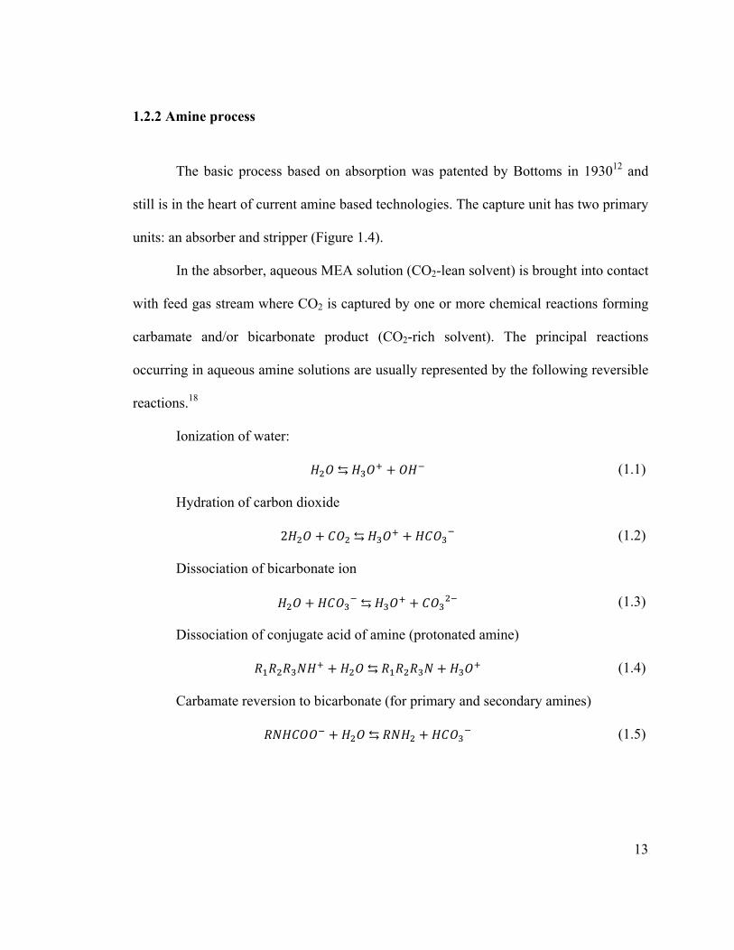
1.2.2 Amine process

The basic process based on absorption was patented by Bottoms in 193012 and

still is in the heart of current amine based technologies. The capture unit has two primary

units: an absorber and stripper (Figure 1.4).

In the absorber, aqueous MEA solution (CO2-lean solvent) is brought into contact

with feed gas stream where CO2 is captured by one or more chemical reactions forming

carbamate and/or bicarbonate product (CO2-rich solvent). The principal reactions

occurring in aqueous amine solutions are usually represented by the following reversible

reactions.18

Ionization of water:

(1.1)

Hydration of carbon dioxide

2 (1.2)

Dissociation of bicarbonate ion

(1.3)

Dissociation of conjugate acid of amine (protonated amine)

(1.4)

Carbamate reversion to bicarbonate (for primary and secondary amines)

(1.5)

14

Figure 1.4 Typical amine-process for CO2 capture.

15

In the stripper, the rich solvent is heated with steam (generated in the re-boiler) to

break down the carbamate/bicarbonate to release CO2. The CO2-lean solution from the

stripper is re-circulated to the absorber and the released high-purity CO2 is compressed

to 100 to 150 bar for geologic sequestration. The reboiler heat duty ( ) required

to release CO2 is an important aspect in determining the cost of amine process. It has

three components, heat of desorpton ); the sensible heat ( required

to rise the temperature of the rich solvent to release CO2 and stripping energy ( .19

(1.6)

16

1.2.3 Effect of chemical reactions on solvent characteristics and cost

Chemical reactions are at the heart of amine-based capture processes and

influence the thermodynamic and kinetic characteristics of the solvent and thus the

process cost. We review the basic theoretical principles that link solvent characteristics

with process economics.

Equilibria and speciation. The maximum quantity (solubility) of a gas

transferred from the vapor phase to a liquid phase in contact, at a certain temperature and

pressure, is determined by the condition of thermodynamic equilibrium (equality of

fugacity or chemical potential of all components in both phases).20 With increase in

pressure, and generally with decrease in temperature, solubility increases. At a certain

temperature and pressure, physical solubility of a certain gas in different solvents varies

due to the differences in the solute-solvent interactions. The thermodynamic equilibrium

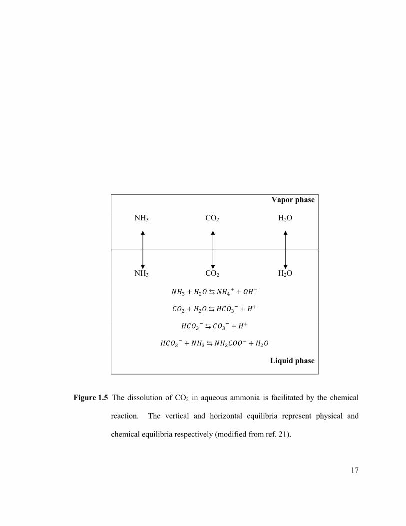
is called physical or chemical depending on whether the solute stays in molecular form

only (physical) or participates into chemically reactions (chemical) (Figure 1.5).

The physical absorption of gases in liquids at low pressure are commonly

quantified in terms of the Henry’s law constant (HLC), usually obtained from

experimental vapor-liquid equilibrium (VLE) measurement or estimation using a

thermodynamic correlation. The HLC of a gas in a solvent at a certain temperature may

be experimentally obtained from the low pressure solubility data as the linear slope of p-

x graph where p is the partial pressure of the gas in the vapor phase and x is its mole

fraction in the liquid phase.

17

Vapor phase

NH3 CO2 H2O

NH3 CO2 H2O

Liquid phase

Figure 1.5 The dissolution of CO2 in aqueous ammonia is facilitated by the chemical

reaction. The vertical and horizontal equilibria represent physical and

chemical equilibria respectively (modified from ref. 21).

18

If the molecular solute reacts with solvent and converts into other chemical

species, HLC decreases and the definition of Henry’s law constant in (1.1) needs to the

modified to take care of the additional driving force for CO2 dissolution (by depletion)

through the corresponding equilibrium constants of all reactions involved (coupled) in

CO2 capture. The mole-fraction based equilibrium constant of the reactions

∏ (1.1) to (1.5) are defined as

(1.7)

where , , and , represent the molefraction-based activity coefficient, mole

fraction, and stoichiometirc coefficient of species present in a reaction. Activity

coefficeint of a species in a liquid mixture is a measure of deviation of its behavior in

that mixtrue from its beahavior in an ideal solution.19

The concentration of captured CO2 is commonly expressed as loading, defined as

mole of CO2 captured in all chemical forms such as carbamte, bicarbonate, carbonate etc.

per mole of amine. The role of chemial reactions on the determination of loading and

absorption capacity is demonstrated in Figure 1.6 with the two most common amines. At

CO2 partial pressure of 0.1 atm (i.e., typical flue gas conditions), the loading in the

primary amime MEA, is more than double than in the tertiary amine MDEA. But, in

terms of absorption capacity, defined as the differnce in rich and lean loading (loading at

typical absorber and stripper conditions respectively, indicated by solid arrow in Figure

1.6), crucial in determining process cost, MDEA has much greater absorption capacity

19

than MEA. The performance of AMP, a sterically hindered primary amine, is in between

that produces mostly bicarbonate and some amount of carbamate (not shown in Figure).

Figure 1.6 Comparison of loading (broken line) and absorption capacity (solid line) of

MEA and MDEA at low pressure. The nubers 1, 2, 3, and 4 represent inlet or

outlet as shown in Figure 1.4. Loading is higher in MEA, but MDEA has

higher absorption capacity (data taken form ref. 19).

0

0.1

0.2

0.3

0.4

0.5

0.6

0.001 0.01 0.1 1 10

Loa

din

g (m

ol/m

ol M

EA

)

Carbon dioxide partial pressure (atm)

40°C, 5M MEA

100°C, 5M MEA

1

2 3

4

0

0.1

0.2

0.3

0.4

0.5

0.6

0.001 0.01 0.1 1 10

Loa

din

g (m

ol/m

ol M

DE

A)

Carbon dioxide partial pressure (atm)

40°C, 5M MDEA

100°C, 5M MDEA

1

2 3

4

20

Absorption capacity or cyclic capacity influences many parameters of the capture

plant and thus influences both the captial cost (CAPEX) and operational cost (OPEX).

An increase in capacity, corresponds to reduction of solvent mass flow rate, that in turn

favorably reduces the following

(i) solvent cost,

(ii) the diameter of the stripper and absorber column

(iii) the heat exchanger size and pumps size and duty (CAPEX) and blower

size

(iv) the sensitive heat ( ) required to rise the temperature rich solvent

inside the stripper defined as19,

ΔΔ

Δ

(1.8)

=liquid heat capacity

=liquid density

= the solvent circulation rate

Δ =different between stripper overhead and reboiler temperature

= concentration of amine in the solvent

=CO2 caputre rate

Δ =difference between loading at the top and bottom of absorption

=loading

Heat of absorption. The total heat of absorption is calculated as the sum of the

individual contributions including the heat of dissolution (physical) of CO2.

Δ (1.9)

21

Reaction rate. Reaction rate, coupled with other factors determines the height of

absorption column. The rate of absorption in a packed absorption column may be

expressed as22,

,,

1 1 (1.10)

The chemical equilibrium influences the concentration of solute in liquid, and

consequently, the driving force for diffusion (the concentration differences, numerator in

equation 1.10). The enhancement factor which is determined by the rate(s) of

chemical reaction(s), signifies the enhancement in absorption rate in addition to physical

solubility ( Henry’s constant, ). The gas and liquid phase mass transfer coefficients,

, and are defined as the ratio of mass flux divided by driving force (difference in

pressure and concentration between bulk and gas-liquid interphase) through the

following equaiton,

(1.11)

where = flux of the solute (quantity of the component transferred per unit time, per

unit area from vapor to liquid phase); and are the partial pressure of solute in main

body of gas adn at interphase; ); and are the concentration of solute in main body of

liquid and at interphase.

The absorption performance (i.e., the height of column necessary to reduce the

concentration of CO2 in the gas phase from 10% to zero) of a number of aqueous amine

solutions of same concentration was tested and, the amines are ranked in the following

22

order: MEA > DEA > AMP > DIPA > MDEA which corresponds with the rate of

reaction of these amines.23

Cost: Ranyanal et al. (2011)24 has identified different capital cost (CAPEX) and

operational cost (OPEX) related to the thermodynamic, kinetic and degradation

characteristics of the solvent for CO2-captrue (90%) from flue gas stream at 1 bar and at

45°C (15% CO2, flow rate 78480 kmol/h) from a 630MW coal-fired power plant using

30wt% MEA that shows that 20%, 39%, 22%, 8%, and 21% of the cost was associated

with heat of reaction, capacity, stripping, kinetics and degradation. 24

23

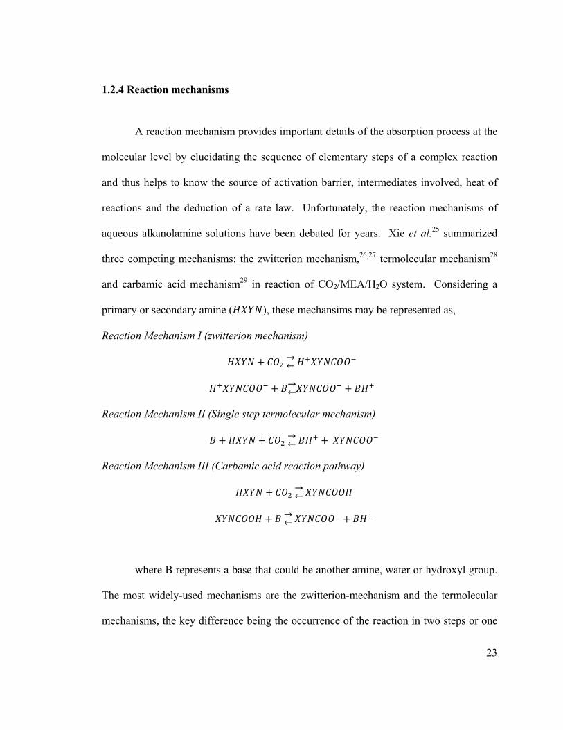
1.2.4 Reaction mechanisms

A reaction mechanism provides important details of the absorption process at the

molecular level by elucidating the sequence of elementary steps of a complex reaction

and thus helps to know the source of activation barrier, intermediates involved, heat of

reactions and the deduction of a rate law. Unfortunately, the reaction mechanisms of

aqueous alkanolamine solutions have been debated for years. Xie et al.25 summarized

three competing mechanisms: the zwitterion mechanism,26,27 termolecular mechanism28

and carbamic acid mechanism29 in reaction of CO2/MEA/H2O system. Considering a

primary or secondary amine ( ), these mechansims may be represented as,

Reaction Mechanism I (zwitterion mechanism)

Reaction Mechanism II (Single step termolecular mechanism)

Reaction Mechanism III (Carbamic acid reaction pathway)

where B represents a base that could be another amine, water or hydroxyl group.

The most widely-used mechanisms are the zwitterion-mechanism and the termolecular

mechanisms, the key difference being the occurrence of the reaction in two steps or one

24

step and the presence/absence of the intermediate called the ‘zwitterion’. Recently,

McCann and coworkers29 have proposed a two-step mechanism where the intermediate

is ‘carbamic acid’ instead of zwitterion.

1.2.5 Basicity of amines

The basicity of amine is quantified by the negative logarithm of the acid

dissociation constant (the pKa) of its conjugate acid (equilibrium constant of equation

1.4). Because it is a fundamental property, it is believed to have impact on all aspects of

CO2/aqueous amine chemistry. A linear correlation between the logarithm of the rate

constant for the formation of zwitterion ( in Equation 1.12) and pKa was found for

primary and secondary alkanolamines. 22

17.6 7188/ (1.12)

The total heat of absorption of CO2 is dominated by equation 1.5. Porcheron et

al. (2011) proposed a screening procedure of amines based on pKa and the pKc (negative

logarithm of the equilibrium constant of carbamate formation reaction).30

For the newer amino-functionalized ionic liquids (FILs), their stability, enthalpy

of absorption, and absorption capacity were controlled by the pKa of ILs,31 and pKa was

also proposed as a criteria to differentiate functionalized ILs from conventional ionic

liquids (ILs).32

25

1.3 IONIC LIQUIDS: PHYSICAL SOLVENT TECHNOLOGY

Room temperature ionic liquid (RTIL) is the generic name of a broad category of

solvents with melting point less than 100°C.33 Ionic liquids are composed of a bulky

organic cation and an organic or inorganic anion. Examples of common cations and

anions are shown in Figure 1.7. The substituent on the cations (the “R” groups) is

typically alkyl chains, but can contain any of a variety of other functional groups as well

(e.g., fluoroalkyl, alkenyl, methoxy, ether, etc.). The asymmetry in shape and bulkiness

in size of the ions results in loosely coordinating packing in ionic liquids responsible for

their low melting point (in contrast to solid NaCl crystal). But the ion-ions interaction in

room-temperature ionic liquids is stronger than other common intermolecular forces

present in organic solvents (e.g., London forces, ion-dipole interaction) that makes it

difficult for them to evaporate, creating no concern for fugitive loss (air pollution) for

process industries. Another appealing property of ionic liquids is their tunability - their

properties can be adjusted by adjusting the constituent ions to suit them for a particular

application. Other advantages include (i) broad liquid window which provides a greater

temperature range to work and (ii) non-flammability, and (iii) supportability on a

membrane. Such versatility has made their prolific growth in a number of potential

engineering applications. 33 However, ionic liquids could be non-biodegradable and/or

toxic that must be assessed before commercial applicaitons.12

26

In a 2009 paper in Nature, researchers at the university of Notre Dame showed

that the solubility of CO2 is very high in certain ionic liquids. This spurred interest to

investigate the possibility of using them in CO2 capture possibly as a physical solvent. 34

Recently, ionic liquids functionalized with reactive amino group or ionic liquids mixed

with amines have been considered for flue gas CO2 capture. 35,36

Some common cation

Some common Anions

Figure 1.7 Common cations and anions in conventional ionic liquids.

27

1.4 SOLVENT DEVELOPMENT

While the chemical landscape of potential solvents is vast, it is often the case that

no single solvent perform better in all desirable characteristics and a trade-off has to be

made. One or more of the following challenges are encountered:

(i) limited cyclic loading capacity of the solvent

(ii) high energy expenditure for solvent regeneration (reduce CO2 from rich

solvent to make lean solvent )

(iii) solvent is corrosive and limits solvent strength (wt% in aqueous solution)

(iv) slow absorption rate due to slow kinetics

(v) solvent is volatile at process conditions, leading to solvent loss and

requiring make-up solvent

(vi) solvent does not have other acceptable physicochemical properties such

as viscosity and operational characteristics

(vii) Solvent degrades with time (oxidative or thermal degradation)

(viii) Solvents (or degradation products) are toxic and not bio-degradable

Therefore, solvent development is a formidable task. The traditional approach

for solvent development is screening experiments followed by thorough investigation on

selected few for comparison with benchmark solvent which is usually the

monoethanolamine (MEA) of similar strength. Many solvents showing promise in early

experiments based on one or more characteristics turn out to be unsuitable later in

thorough investigation. One recent example is the fate of 3-(methylamino)propylamine

28

(3-MAPA) that showed promise in early studies (e.g., Kim et al. (2008))37 which later

was found not suitable when other properties were also considered (Voice et al.

(2013))38. Another example is that of 2-((2-aminoethyl) amino) ethanol (AEEA), which

was initially found to have both higher CO2 absorption rate and higher cyclic capacity

than those of MEA by a screening experiment39, but was later found to have problem

with degradation (thermally degrade at high temperature)40. Solvent development

through experimental screening of large number of possible solvents thus requires

significant experimental efforts.

Quantum-mechanical computational tools can be valuable in understanding

solvent chemistry and to develop new solvents.41 One computes chemical results either

as an alternative or complementary to experimental method for the following reasons.42

Accessibility

Economy

Understanding

Computation can reduce the cost and time for experiment by providing reliable a

priori guidelines. Computation also allows studying solvents not yet synthesized. For

example, Zhang et al. (2008) studied more than 700 ionic liquids virtually prepared

computationally, and then finally did measurement on selected few.43 Chemical

reactions in aqueous amine solutions are difficult to study experimentally due to

coupling of multiple reactions; and their fast nature makes it difficult to get mechanistic

details, therefore justifying using theory and computation for such study.44

Computational studies are suitable for interpreting phenomena at the molecular level that

29

help build novel solvent. For example, the computational mechanistic study of reaction

of amine with CO2 of Mindrup and Schneider (2009)45 led to the development of a

functionalized ionic liquid35 with high capture capacity (1 mole CO2 per mole of IL).

Similarly, computational study46 of the interaction of CO2 with the amino group led to

the development of two new TSILs47 with high absorption capacity.

1.5 OBJECTIVES AND SCOPE

The objectives of this dissertation is to use molecular modeling tools to predict

pKa of aqueous amines, address the CO2-capture mechanism debate and screen ionic

liquids as alternatives to aqueous amines as well as to measure (experimentally) the

solubility of CO2 in promising ionic liquids and thermophysical properties of an

important mixed solvent.

Due to the possible influence of basicity of amines on all aspects of CO2/amine

chemistry, an efficient computational protocol was developed to predict pKa (Chapter 3)

of amines of interest in CO2-capture. The pKa of some amines at 25°C were

experimentally measured to test the method. This method was contrasted with a pencil-

and-paper method based on linear free energy relationship. Reaction mechanisms for the

formation of carbamate and bicarbonate were studied to provide further fundamental

insight into the capture process, solve the debate over carbamate formation mechanism

and to study the effect of basicity on the mechanism of various amines. This work was

divided into two parts: static calculations (0 K) and dynamic calculations (313 K),

30

presented in Chapters 4 and 5 respectively, using computational tools of different levels

of sophistication (Chapter 2).

Room temperature ionic liquids (RTILs) for applications in CO2 separation from

flue gas or natural gas streams are computationally screened from a large database using

Henry’s law constant as screening criteria. The ‘structure-activity’ relationships are

explored to see how the properties of ILs affect the solubility and selectivity (Chapter 6).

Solubility of CO2 in three ionic liquids selected based on the screening study was

measured (Chapter 7) at (283.15,298.15 and 323.15) K and at (0.5 to 2) MPa. The data

were correlated with Peng-Robinson equation of state. The experimentally derived

Henry’s law constant was compared with COSMO-RS prediction.

In Chapter 8, the thermo-physical properties (density, viscosity, and excess

enthalpy) of aqueous solution of promising ionic liquid, 1-butyl-3-methyl imidazolium

acetate, [bmim][Ac], were studied. Excess enthalpy of ([bmim][Ac] + water) system at

25°C was compared with some (amine + [bmim][Ac]) systems.

31

1.6 REFERENCES

1. Maginn, E. J. What to Do With CO2? J. Phys. Chem. Lett. 2010, 1, 3478.

2. Stern, M. C.; Simeon F.; Herzog, H.; Hatton, T. A. Post-Combustion Carbon

Dioxide Capture Using Electrochemically Mediated Amine Regeneration.

Energy Environ. Sci. 2013, 6, 2505.

3. Li, B.; Duan Y.; Luebke D.; Morreale B. Advances in CO2 Capture Technology:

A patent review. Appl. Energy 2013, 102, 1439.

4. Scripps Institution of Oceanography (Scripps) and the National Oceanic and

Atmospheric Administration (NOAA)) (Available from:

http://CO2now.org/Current-CO2/CO2-Now/noaa-mauna-loa-CO2-data.html

Accessed June 23, 2013).

5. National Oceanic and Atmospheric Administration (NOAA) (Available from:

http://www.ncdc.noaa.gov/cag/time-series/global, (Accessed June 23, 2013).

6. Metz, B.; Davidson, O; de Coninck, H. C.; Loos; M.; Meyer, L. A. editors. IPCC

Special Report on Carbon Dioxide Capture and Storage. Prepared by Working

Group III of the Intergovernmental Panel on Climate Change. New York:

Cambridge University Press; 2005.

7. Dooley, J. J.; Davidson, C. L.; Dahowski, R. T. An Assessment of the

Commercial Availability of Carbon Dioxide Capture and Storage Technologies

as of June 2009. Pacific Northwest National Laboratory, U.S.DOE. 2009.

32

8. Hedin, N.; Andersson, L.; Bergström, L.; Yan, J. Adsorbents for the Post-

Combustion Capture of CO2 Using Rapid Temperature Swing or Vacuum Swing

Adsorption. Appl. Energy 2013, 104, 418.

9. Habib, M. A.; Nemitallah, M.; Ben-Mansour, R.. Recent Development in Oxy-

Combustion Technology and its Applications to Gas Turbine Combustors and

ITM Reactors. Energy Fuels 2013, 27, 2.

10. van Bergen, F.; Gale, J.; Damen, K. J.; Wildenborg, A. F. B. Worldwide

Selection of Early Opportunities for CO2-EOR and CO2-ECBM. Energy 2004,

29 , 1611.

11. Zakkour, P.; Cook, G. CCS Roadmap for Industry: High-purity CO2 Sources.

Carbon Counts Company (UK) Ltd., September, 2010.

12. Ramdin, M.; de Loos, T. W.; Vlugt, T. J. H. State-of-the-Art of CO2 Capture

With Ionic Liquids. Ind. Eng. Chem. Res. 2012, 51, 8149.

13. Kohl, A. L.; Nielsen, R. B. Gas Purification. (5th ed.). Gulf Professional

Publishing: Houston, 1997.

14. Yildirim, Ö.; Kiss, A. A.; Hüser, N.; Leßmann, K.; Kenig, E. Y. Reactive

Absorption in Chemical Process Industry: A Review on Current Activities.

Chem. Eng. J. 2012, 213, 371.

15. Rubin, E. S.; Mantripragada, H.; Marks, A.; Versteeg, P.; Kitchin, J. The Outlook

for Improved Carbon Capture Technology. Prog. Energy Combust. Sci. 2012,

38, 630.

16. Rochelle, G. T. Amine Scrubbing for CO2 Capture. Science 2009, 325, 1652.

33

17. Toth, F.L. Geological Disposal of Carbon Dioxide and Radioac-tive Waste: A

Comparative Assessment. Springer Verlag, Netherlands, 2011.

18. Kim, I.; Hoff, K. A.; Hessen, E. T.; Haug-Warberg T.; Svendsen, H. F. Enthalpy

of Absorption of CO2 With Alkanolamine Solutions Predicted From Reaction

Equilibrium constants. Chem. Eng. Sci. 2009, 64 , 2027.

19. Meldon, J. H. Amine Screening for Flue Gas CO2 Capture at Coal-Fired Power

Plants: Should the Heat of Desorption be High, Low or in Between? Curr. Opin.

Chem. Eng., 2011, 1, 55.

20. Prausnitz, J. M.; Lichtenthaler, R. M.; de Azevedo, E. G. Molecular

Thermodynamics of Fluid Phase Equilibria (3rd ed.). Prentice-Hall, Englewood

Cliffs, NJ. 1998.

21. Göppert, M.; Maurer G. Vapor-Liquid Equilibria in Aqueous Solutions of

Ammonia and Carbon Dioxide at Temperatures Between 333 and 393 K and

Pressures up to 7 MPa. Fluid Phase Equilib., 1988, 41, 153.

22. Versteeg, G. F.; van Dijck, L. A. J.; van Swaaij, W. P. M. On the Kinetics

between CO2 and Alkanolamines Both in Aqueous and Non-aqueous Solutions.

An Overview. Chem. Eng. Commun. 1996, 144, 113.

23. Aroonwilas, A.; Veawab, A.; Tontiwachwuthikul, P. Characterization and

Comparison of the CO2 Absorption Performance Into Single and Blended

Alkanolamines in a Packed Column. Ind. Eng. Chem. Res. 2004, 43, 2228.

34

24. Raynal, L.; Bouillon, P. A.; Gomez, A.; Broutin, P. From MEA to Demixing

Solvents and Future Steps, a Roadmap for Lowering the Cost of Post-

Combustion Carbon Capture. Chem. Eng. J. 2011, 171, 742.

25. Xie, H.; Zhou, Y.; Zhang, Y.; Johnson, J. K. Reaction Mechanism of Mono-

ethanolamine With CO2 in Aqueous Solution from Molecular Modeling. J. Phys.

Chem. A 2010, 114, 11844

26. Caplow, M. Kinetics of Carbamate Formation and Breakdown. J. Am. Chem.

Soc. 1968, 90, 6795.

27. Danckwerts, P. V.The Reaction of CO2 With Ethanolamines. Chem. Eng. Sci.

1979, 34, 443.

28. Crooks, J. E.; Donnellan, J. P. Kinetics and Mechanism of the Reaction between

Carbon Dioxide and Amines in Aqueous Solution. J. Chem. Soc., Perkin Trans.

2, 1989, 331.

29. McCann, N.; Phan, D.; Wang, X.; Conway, W.; Burns, R.; Attalla, M.; Puxty, G.;

Maeder, M. Kinetics and Mechanism of Carbamate Formation from CO2(aq),

Carbonate Species, and Monoethanolamine in Aqueous Solution. J. Phys. Chem.

A 2009, 113, 5022.

30. Porcheron, F.; Gibert, A.; Mougin, F.; Wender, A. High Throughput Screening of

CO2 Solubility in Aqueous Monoamines Solutions. Environ. Sci. Technol. 2011,

45, 2486.

35

31. Wang, C.; Luo, X.; Luo, H.; Jiang, D.-E.; Li, H. and Dai, S. Tuning the Basicity

of Ionic Liquids for Equimolar CO2 Capture. Angew. Chem. Int. Ed., 2011, 50,

4918.

32. Ren, S. H.; Hou, Y. C.; Tian, S. D.; Chen, X. M.; Wu, W. Z.What are Functional

Ionic Liquids for the Absorption of Acidic Gases? J. Phys. Chem. B 2013, 117,

2482.

33. Brennecke, J. F. and Maginn, E. J. Ionic liquids: Innovative Fluids for Chemical

Processing. AIChE J., 2001, 47: 2384.

34. Blanchard, L. A., Hancu, D., Beckman, E..J., Brennecke, J. F., Green Processing

Using Ionic Liquids and CO2. Nature 1999, 399, 28.

35. Gurkan, B. E.; de la Fuente, J. C.; Mindrup, E. M.; Ficke, L. E.; Goodrich, B. F.;

Price, E. A.; Schneider, W. F.; Brennecke, J. F. Equimolar CO2 Absorption by

Amine-Functionalized Ionic Liquids. J. Am. Chem. Soc. 2010, 132, 2116

36. Camper, D.; Bara, J. E.; Gin, D. L.; Noble, R. D. Room-Temperature Ionic

Liquid Amine Solutions Tunable Solvents for Efficient and Reversible Capture of

CO2. Ind. Eng. Chem. Res. 2008, 47, 8496.

37. Kim, I., Svendsen, H. F., Børresen, E., Ebulliometric Determination of Vapor–

Liquid Equilibria for Pure Water, Monoethanolamine, N-Methyldiethanolamine,

3-(Methylamino)-Propylamine, and their Binary and Ternary Solutions. J. Chem.

Eng. Data 2008, 53 , 2521.

36

38. Voice A. K.; Vevelstad S. J.; Chen X.; Nguyen T., Rochelle G. T.; Aqueous 3-

(methylamino)propylamine for CO2 Capture. Int. J. Greenhouse Gas Control

2013 15, 70.

39. Ma'mun, S.; Jakobsen, J. P.; Svendsen, H. F.; Juliussen, O. Experimental and

Modeling Study of the Solubility of Carbon Dioxide in Aqueous 30 Mass % 2-

((2-Aminoethyl)amino)ethanol Solution. Ind. Eng. Chem. Res. 2006, 45, 2505.

40. Davis, J.; Thermal Degradation of Aqueous Amines Used for Carbon Dioxide

Capture. Ph.D. Dissertation. The University of Texas, Austin, USA, 2009.

41. Maiti, A.; Bourcier W. L.; Aines, R. D. Atomistic Modeling of CO2 Capture in

Primary and Tertiary Amines – Heat of Absorption and Density Changes.

Chem.Phy. Lett. 2011, 509, 25.

42. Almlöf, J. Electronic Structure Theory. In Mathematical Frontiers in

Computational Chemical Physics, Truhlar D.G. Ed; Springer-Verlag, 1988; Vol.

15; p 18.

43. Zhang, X.; Liu, Z.; Wang, W. Screening of Ionic Liquids to Capture CO2 by

COSMO-RS and Experiments. AIChE J. 2008, 54, 2717.

44. Gallet, G. A.; Pietrucci, F.; Andreoni, W. Bridging Static and Dynamical

Descriptions of Chemical Reactions: an Ab Initio Study of CO2 Interacting With

Water Molecules. J. Chem. Theory Comput. 2012, 8, 4029.

45. Mindrup, E. M.; Schneider, W. F. Computational Comparison of Tethering

Strategies for Amine Functionalized Ionic Liquids. In ACS Symposium Series;

Seddon, K.; Rogers, R.; Plechkova, N., Eds.; American Chemical

Society: Washington, D.C., 2009, p 419.

37

46. Yu, G.; Zhang, S.; Yao, X.; Zhang, J.; Dong, K.; Dai, W.; Mori, R. Design of

Task-Specific Ionic Liquids for Capturing CO2: A Molecular Orbital Study. Ind.

Eng. Chem. Res. 2006, 45, 2875.

47. Zhang, J.; Zhang, S.; Dong, K.; Zhang, Y.; Shen, Y. ; Lv, X. Supported

Absorption of CO2 by Tetrabutylphosphonium Amino Acid Ionic Liquids.

Chem. -Eur. J. 2006, 12, 4021.

38

Chapter 2: Computational Methods _______________________________________________________________________

2.1 INTRODUCTION

Modeling bulk properties of a liquid phase has always been a challenge as they

arise from statistical behavior of a vast number of molecules, whose behavior, in turn,

stem from their electronic structure. The quest for the foundation of macroscopic

behavior of fluids in the microscopic realm of molecular properties (e.g., van der Waals

equation of state (1873)) 1 started at a time when even the existence of molecules was not

widely recognized. Today, more than a century later, such quest has turned into the

industrial practice of designing products from electronic level of matter.

Thermodynamic models have much evolved since van der Waals.

Thermodynamic models of liquid for industrial design and simulation (e.g., UNIFAC2 in

1975, SAFT3 in 1989) were developed by exploiting the link between macroscopic and

microscopic properties through classical statistical mechanics. More recently,

thermodynamic models with direct root at the electronic structure calculations appeared (

e.g., COSMO-RS (1995))4 and their applications to various chemical engineering

problems was facilitated by the engineers’ access to quantum-mechanical computational

tools (the application of quantum mechanics as a ‘new tool for engineering

thermodynamics’ was reviewed by Sandler (2003)5). The introduction of quantum

39

mechanics is necessary to treat the electronic structure of matter (because no classical

analog is present for it); and also for the ab initio (from the first principle) treatment of

atoms and molecules. John Pople and Walter Kohn received Nobel prize for their

contribution in making quantum-mechanical calculations possible for practical chemical

problems in 1998 (about 90 years later van der Waals received Nobel prize in 1910). At

present, with advancement in computer technologies, many powerful computational

tools have been developed that generally belong to the area of molecular modeling (also

known as computational chemistry).

2.2 MOLECULAR MODELING

“Molecular modeling is nowadays a well-established analytical tool exactly as

spectroscopies or other experimental methodologies, and we expect that its impact on

many research fields in chemistry, biology, material science, and even medicine will

enormously increase in the near future”.6 Molecular modeling provides a set of

techniques based on the principles of classical and quantum physics to compute chemical

and thermodynamic properties such as geometry, reactivity, reaction mechanisms,

spectra etc of a molecule or a system of molecules.7 The major tools of computational

chemistry (also termed as ‘molecular modeling’) include

Molecular mechanics methods,

Ab initio methods,

Semiempirical methods,

Density functional theory (DFT) methods and

40

Molecular dynamics methods.7

Selection of one or more methods depends on the nature of problem and the

chemical information sought. These methods are being increasingly applied by

researchers in the area of CO2 capture. We have used Ab initio and DFT based methods

for static calculations as well as molecular dynamics methods for dynamic calculations

in this dissertation to solve different aspects relevant to solvent development. We briefly

provide the overview of some key elements of quantum chemistry (The Schrodinger

equation, potential energy surface), basic computational methods and models frequently

used in molecular modeling below.

2.2.1 Schrodinger equation (SE)

Quantum-mechanics describes the state of a molecular system by a function that

depends on the coordinates and spin of the particle and time. This function is called the

wave function and contains all the information about the system.

Ψ Ψ coordinates and spin of all particles, time

The wave function is obtained by solving the Schrodinger equation (SE). In molecular

modeling, the time-independent, non-relativistic treatment of Schrodinger equation

(Equation 2.1)8 is normally sufficient.

Ψ , Ψ , (2.1)

Where H is the Hamiltonian operator, is energy and Ψ is the wave function. R and r

represent the set of spatial coordinates of the nuclei and electrons respectively. The spin-

dependence of wave function is introduced in an ad hoc manner in non-relativistic

41

treatment of Schrodinger Equation. Equation (2.1) is an eigen value equation as it has

the form where an operator acts on the wave function to produce a constant times the

wave function. Any physically observable quantity can be calculated from the wave

function with a corresponding eigen value equation using the corresponding quantum-

mechanical operator.

The Hamiltonian operator is formulated from the classical expression for kinetic

and potential energy. For a molecule in vacuum, the Hamiltonian ( ) consists of five

other operators associated with the kinetic ( ) and potential energy ( ) of the particles.

(2.2)

The subscripts ‘n’ and ‘e’ in equation (2.2) denotes nucleus and electron respectively;

and the five operators on the RHS of equation (2.2) are associated with kinetic energy of

nuclei ( ), kinetic energy of electrons ( ), electron-nuclei attraction ( ), neucleus-

neucleus repulsion ( ) and electron-electron repulsion ( ). The Hamiltonian is

augmented by additional terms if the system is in any external potential field (for

example to mimic the presence of solvents around a solute) or if other quantum-

mechanical or relativistic effects are necessary.

Since electrons are much lighter than the nuclei, the nuclear velocities are much

smaller than those of electrons. Thus, electrons adjust to nuclear motion instantly and

essentially see the nuclei as stationary. This enables to decouple the motions of electrons

from that of nuclei and thus Schrodinger equations can be applied for electrons and

nuclei separately. The electronic Schrodinger equation is written for fixed or clamed

nuclei as8

42

; Ψ ; Ψ ; (2.3)

where ; (later denoted as ) is the electronic energy

(with reference state at infinitely separated electrons and nuclei and at rest) of the system

and depends functionally on the spatial coordinates of the electrons, but only

parametrically on the nuclear coordinates. This approximation is known as Born-

Oppenheimer approximation.

2.2.2 Potential energy surface (PES)

Definition. Equation 2.3 is the cornerstone of computational chemistry and it

represent the energy-geometry relationship of a molecule or a group of molecules (The

BO approximation implies that a molecule has a shape or geometry defined by the

positions of the coordinates of the nuclei; electronic coordinates are not necessary to

define geometry as since the electron will adjust their motion instantly with a given

nuclear position). By plotting the energy (solutions of equation 2.3 for many given

nuclear configurations) as a function of nuclear coordinates (R), one obtains the

potential energy surface of the system. It may be mentioned that for each nuclear

configuration, many wave functions, each associated with an associated energy, will

satisfy equation 2.3, and among them, the one associated with lowest energy, called

ground-state energy are used in plotting the ground-state PES.

43

Dimensionality. For N atoms, 3N dimensions are required to define the

geometry; and leaving out the 6 degree of motion for overall (center-of-mass)

translational and rotational motion, there are 3N-6 degrees left for relative internal

movement of the nuclei. Therefore, the PES of a N-atom molecule with stationary or

frozen nuclei requires 3N-6 (or 3N-5 for linear molecules) nuclear coordinates. Different

possible geometries of a molecule can also be expressed in terms of internal coordinates

such as distance between two nuclei, angle among three nuclei, and dihedral angel

among four nuclei instead of the Cartesian coordinates of each nucleus.9 Mathematically,

the PES is thus the following multidimensional function,

, , … , (2.4)

Where, the , , . . are internal coordinates.

Stationary points. Due to large dimensionality of the complete PES for practical

systems, it is difficult to obtain information of full PES, rather one focuses on the

chemically relevant part of it (such as minima, maxima, saddle point).10 For example,

information of a bond breaking or forming during chemical reaction is obtained by

observing energetic variation along the coordinates directly involved. A minimum on

PES corresponds to a chemically stable configuration and the lowest energy path (also

called intrinsic reaction coordinate, IRC) connecting two minimum through a maxima

corresponds to an elementary reaction step (Figure 2.1); the minima could be

reactants/products/intermediate and the maximum is the transition state (TS) structure.

An ‘intermediate’ is a short-lived compound that may be isolated; whereas a TS has only

momentary existence. The value of the reaction coordinate (e.g., a bond length) in TS is

between the values of the coordinate in the two connecting minima; and such proximity

44

defines an early vs. late TS). The energy difference between a reactant and the transition

state of an elementary step is the activation energy of the step and the reactant will pass

over the maxima if it acquires kinetics energy higher than the activation energy.

Stationary points on a PES are identified with the following criteria.7

At a stationary point, 0 for all geometric coordinates (i.e. 0)

At a minimum, 0 for all geometric coordinates (along all directions) and

0 for all (along all directions)

For a transition state, 0 for all geometric coordinates (along all directions); and

0 for =the reaction coordinate, but 0 for all other (along all other

directions).

45

Figure 2.1 A one-dimensional projection of a potential energy surface showing the IRC

for a reaction that connects two minima.

46

Zero point energy. Calculations to locate minima and transition states on a PES

that requires the computations of first and second derivatives of energy with respect to

all the internal coordinates as discussed above and such calculations are called geometry

optimization. An initial geometry is given and the program moves the geometry towards

a stationary point using different numerical algorithms (e.g., Berny algorithm). Once a

minima or transition state is found, an additional frequency calculation is carried out to

get additional insight into the nature of that geometry (for example, to identify the

particular reaction coordinate involved in IRC). Such calculations find the normal-mode

frequency of all the modes of vibration (atoms vibrate even at 0 K and the associate

energy is called zero-point energy; the frozen-nuclei coordinates of the atoms on a PES

corresponds to the equilibrium position of such vibration). In a minima, all the bonds

vibrate periodically, a restoring force acts on the nuclei whenever it is out of equilibrium

position to bring it back to equilibrium; but in a transition state, one of the vibration will

occur without the restoring force, and therefore, it many fall to either direction towards

the reactants or products along the IRC.

47

2.2.3 Solving the electronic schrodinger equation

As mentioned earlier, geometry optimization (finding minima, TS on a PES)

requires the computation of electronic energy of the system for clamped nuclei by

solving equation (2.2). Methods for solving this equation are based on two types of

theory: the wave function theory (WFT) and the density functional theory (DFT). WFT-

based methods are called ab initio (from beginning) or first principle methods because

they use only the fundamental constants and do not use any experimental data directly.

In DFT-methods, ground-state energy is computed from ground-state electron density,

utilizing some notions of WFT to facilitate computation of the ground-state density.

Selection of a method depends on the trade-off between the two desired levels of cost

and accuracy.

Ab initio methods. All ab initio methods require the representation of the

complex N-electronic wave function (Ψ of equation 2.3) that depends on 4N variables

(three spatial coordinates and spin of each of the N electrons) by a number of simpler 1-

electron wave functions, known as spin-orbitals, that depends on 4 variables. This step,

that determines the mathematical relationship between the electronic wave function and

spin-orbitals (sprout) engenders many ab initio methods (discussed later).

Each spin-orbital is product of two functions, the molecular orbital (depends on the 3

coordinates of the electron) and the spin function (depends on the spin of the same

electron). Each of molecular orbital is further by linear combinations of some predefined

basis functions, representing the atomic orbitals of the constituent atoms.

48

; (2.5)

where, is the -th the basis function in the -th molecular orbital ( ); is the

corresponding coefficient. Thus, in effect, the problem of determining the wave function

turns into finding these coefficients (an easier numerical problem). The set of the basis

function is called a basis set (discussed later). The nature and number of basis functions

must be selected judiciously commensurate with a method and nature of chemical

interaction present. The method (also called ‘level of theory’) and basis-set chosen for a

problem together are called ‘model chemistry’.

Once an approximate mathematical form of the wave function is determined, the energy

is obtained from the newly constructed wave function by the postulates of quantum

mechanics (equation 2.6).

Ψ | |ΨΨ |Ψ

(2.6)

Equation (2.8) is written in the bra-ket notation used to represent multi-dimensional

integrals. Explicitly,

Ψ| |Ψ Ψ Ψ d (2.7)

Ψ |Ψ Ψ Ψ d (2.8)

where the integral sign represents multiple integration over all spatial variables and

summation over all spin variables. Ψ represents the complex conjugate of the function

Ψ (e.g., Ψ x iy if Ψ x iy , etc).

Finally, the variational principle, that any approximate wave function will always give

ground state energy higher than the true ground-state energy, is invoked and wave

49

function that corresponds to lowest possible energy is sought. An objective function by

means of Lagrange multipliers is constructed that additionally ensures that molecular

wave function be orthonormal (a property required of wave functions).

,

(2.9)

The objective function can also be formulated into basis functions using equation

(2.7) and then minimized. Minimization of equation (2.11) ( 0 ) leads to the a set of

equations that are solved iteratively and the solutions provide the molecular orbitals ,

orbital energies (the constant in equation 2.11 is generally interpreted as the energy

of orbital , designated as ) and the total electronic energy.

The basic scheme described above is common to all ab initio methods. They

differ in their construction of the approximate form of Ψ as a composite function of

spin-orbitals, (discussed before). Such construction has implication on the level of

rigor of the treatment of the quantum-mechanical nature of electronic motion in presence

of other electrons; rigorous treatment requires deployment of more molecular orbitals (to

represent many possible electronic configuration), but this increases the computational

cost.

The basic ab initio method is the Hartree-Fock (HF) method that satisfies some

crucial aspects of quantum-mechanical nature of electron motion (but not all) and the

starting point for more accurate (post-HF method) or less accurate (semiempirical)

methods. For a closed shell system (no unpaired electrons), the HF method approximates

the wave function with a single determinant called Slater determinant.

50

Ψ ~ΦSD (2.10)

ΦSD √N!

1 12 2

… 1… 2

…

; ;1,0, (2.11)

The Slater determinant is constructed from N spin-orbitals for a N-electron

closed-shell system, which is the minimum number of orbitals for its ground state

electronic configuration. Mathematical properties of Slater determinant automatically

accounts for the quantum-mechanical Pauli Exclusion Principle. Two-electrons may

occupy the same space only if they have opposite spin. Thus, the N spin-orbitals in the

Slater determinant are constructed from N/2 spatial orbital, each of them occupy two

electrons with different spin. If m basis functions are used, a total of m spatial molecular

orbitals are constructed by linear combination with different coefficients (a total of

coefficients arising from a mxm matrix). Out of the m molecular orbitals, only N/2

orbitals are occupied (filling in orbitals in ascending order of their energies), and the

remaining orbitals are called unoccupied or virtual orbitals. The energy difference

between the highest occupied molecular orbital (HOMO) and lowest unoccupied

molecular orbitals (LUMO), are important in the study of chemical reaction (HOMO and

LUMO, altogether are called frontier orbitals).

In Hartree Fock method, the electron-electron repulsion is treated in an average

manner: the ‘electron-electron’ repulsion is replaced with ‘electron-average field’

repulsion where the average electric field is generated by all other electrons and the bare

nuclei (instead of one to one electron-electron interaction). But the motion of an electron

at any instant is dynamically correlated with the motion of every other electrons. This

51

‘correlation energy’ (sometimes defined as the difference between the lowest possible

energy obtainable and the HF energy obtained by a given basis set) is treated in a better

way by Post-Hartree Fock methods. One such method is ‘MP2’ based on Moller-Plesset

(MP) perturbation theory where the HF energy is corrected to first order by adding the

‘correlation energy’ as a first order correction. Ψ is expanded into many wave functions

around the wavefunction of a reference system that can be treated very accurately.

Ψ Ψ Ψ .. (2.12)

The energy of the reference system is designated as MP0 and may be computed

very accurately, then corrections of increasing order are added to it (the corrected energy

is designated as MP1, MP2, MP3, MP4 etc). MP1 energy is the Hartree-Fock energy and

MP2 energy is the first correction beyond HF that is computed by promoting electrons

from occupied to unoccupied orbitals, in some sense, giving them more room to avoid

one another, thus recovering some part of the dynamic correlation.7

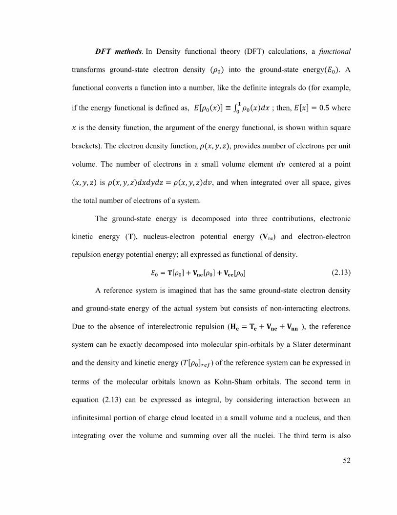
52

DFT methods. In Density functional theory (DFT) calculations, a functional

transforms ground-state electron density into the ground-state energy . A

functional converts a function into a number, like the definite integrals do (for example,

if the energy functional is defined as, ; then, 0.5 where

is the density function, the argument of the energy functional, is shown within square

brackets). The electron density function, , , , provides number of electrons per unit

volume. The number of electrons in a small volume element centered at a point

, , is , , , , , and when integrated over all space, gives

the total number of electrons of a system.

The ground-state energy is decomposed into three contributions, electronic

kinetic energy (T), nucleus-electron potential energy (Vne) and electron-electron

repulsion energy potential energy; all expressed as functional of density.

(2.13)

A reference system is imagined that has the same ground-state electron density

and ground-state energy of the actual system but consists of non-interacting electrons.

Due to the absence of interelectronic repulsion ( ), the reference

system can be exactly decomposed into molecular spin-orbitals by a Slater determinant

and the density and kinetic energy ( ) of the reference system can be expressed in

terms of the molecular orbitals known as Kohn-Sham orbitals. The second term in

equation (2.13) can be expressed as integral, by considering interaction between an

infinitesimal portion of charge cloud located in a small volume and a nucleus, and then

integrating over the volume and summing over all the nuclei. The third term is also

53

approximated as classical coulomb interaction between two charge cloud within two

separate infinitesimal volume elements and then integrating over the volume elements.

This electron-electron energy and the kinetic energy of the reference system is not same

as the energy for true system due to electron correlation, and the deviation is corrected

by a term called exchange-correlation energy ( ) . These consideration lead to the

total energy of actual system,

(2.14)

The exchange-correlation energy, , is unknown and different DFT-methods

differ in the approximate expression used for this functional. Using a suitable expression

for , constraint minimization of the ground state energy (equation 2.14) lead to the

solution of spatial molecular orbitals known as Kohn-Sham (KS) orbitals. The electron

density for a N electron closed shell system is computed as,

1 (2.15)

The approximate functional used in practical calculations are developed by

appealing to theoretical models and contain parameters that are fitted to experimental

data. These functionals are written as a summation of two parts, the exchange part

(dominating) and a correlation part ( ). In hybrid DFT method, another

possible improvement is to use a weighted sum of HF exchange energy and the DFT

exchange-correlation energy. The exchange-correlation functional also prevents

analytical solution of the integrals. The combination of three-parameter exchange

functional of Becke (1988) (abbreviated as B3) with the correlation functional of Perdew

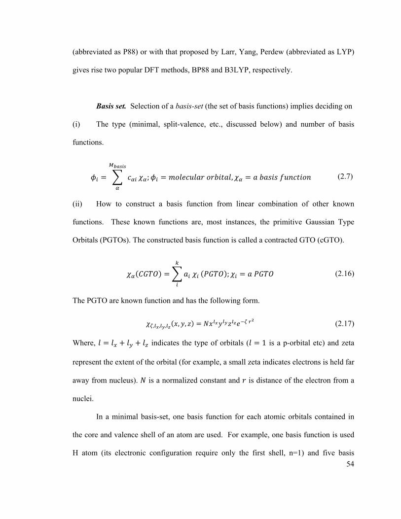
54

(abbreviated as P88) or with that proposed by Larr, Yang, Perdew (abbreviated as LYP)

gives rise two popular DFT methods, BP88 and B3LYP, respectively.

Basis set. Selection of a basis-set (the set of basis functions) implies deciding on

(i) The type (minimal, split-valence, etc., discussed below) and number of basis

functions.

; , (2.7)

(ii) How to construct a basis function from linear combination of other known

functions. These known functions are, most instances, the primitive Gaussian Type

Orbitals (PGTOs). The constructed basis function is called a contracted GTO (cGTO).

; (2.16)

The PGTO are known function and has the following form.

, , , , , (2.17)

Where, indicates the type of orbitals ( 1 is a p-orbital etc) and zeta

represent the extent of the orbital (for example, a small zeta indicates electrons is held far

away from nucleus). is a normalized constant and is distance of the electron from a

nuclei.

In a minimal basis-set, one basis function for each atomic orbitals contained in

the core and valence shell of an atom are used. For example, one basis function is used

H atom (its electronic configuration require only the first shell, n=1) and five basis

55

functions are used for carbon, nitrogen or oxygen atom (their electronic configuration

require two shells, n=1 and n=2; and one basis function is allotted for each orbital in

these shell).

In a Split-valence basis set, one basis function for each of the core orbitals

(orbitals in the inner shells shell in an atom), more than one (two, three, four etc) basis

functions for each valence orbitals (orbitals in the outermost shell from nucleus) are

used. Thus, double-zeta, triple-zeta, quadruple-zeta respectively refer to the use of two,

three and four basis functions for representing the valence orbitals. For example, a split-

valence double zeta basis set uses two basis functions for hydrogen (for the 1s valence

orbital), and nine functions for carbon, nitrogen, and oxygen atoms (two functions for

each of the four orbitals in the second shell plus one for the core 1s orbital).

Split-valence basis set developed by Pople and coworkers are usually expressed

by acronyms such as ‘k-nlG’ (e.g., 6-31G). The numeral ‘k’ indicates the number of

PGTOs used to represent the core orbitals. The two numerals after the dash indicate a

double split valence orbitals respectively where ‘n’ and ‘l’ PGTOs will be used to

represent the first and second set of splited valence orbitals. PGTOs in these two sets

have different values of zeta and thus their linear combination allows for the possibility

for orbitals to be of different size. Similarly, ‘k-nlmG’ (e.g., 6-311G) represents split-

valence triple zeta basis set and can provide further flexibility in orbital sizes.

An orbital can be represented as a mixed orbital by adding other type of orbitals

to it. Adding polarization function to split-valence double zeta basis set generates the

‘polarized double-zeta’ basis set. Polarization functions add additional flexibility to an

orbital by permitting its electrons to be displaced in a certain direction necessary for an

56

interaction (for example when two atoms approach). They are denoted by a single

asterisk (*) if polarization function is added only to heavy atoms (atoms except H and

He) and double asterisk (**) is used to indicate polarization of all atoms. Instead of

asterisk the added orbitals is also used in the acronym. For example, 6-31G(d) or 6-31G*

indicate the same basis-set (add 6 d-orbitals to each of the valence orbitals of heavy

atom). To generate significant electron density far away from nucleus for example

necessary for an anion, diffuse functions can be added. They are expressed as (+ for

‘heavy atom’ or ++ for all atom) before the letter G in a split-valence basis set.

The basis-sets mentioned above are optimized at Hartree-Fock level.

‘Correlation-consistent split-valence’ basis sets were developed by Dunning and

coworkers by optimizing those using correlated wave functions for applications in post-

Hartree Fock methods. They are abbreviated as cc-pVXZ stands for correlated-

consistent polarized valence X zeta basis set with X=D, T,Q etc for double, triple,

quadruple split valence basis set.

The basis set mentioned above are atom-centered, and they originate with

reference to the orbitals for the simplest one-electron system, the hydrogen atom, for

which equation (2.2) can be exactly solved and the corresponding one-electron wave

functions are analytically known.8 Instead of building MOs from AOs which in turn

from PGTOs, one can build MOs directly from plane waves, without reference to AOs.

These waves stem from the solution of SE for a free electron.

. (2.18)

57

is a wave vector that play the same role as zeta is a GTO and is related to energy

(momentum of the wave, and energy, 2⁄ where, is the mass of

an electron;). They greatly simplifies calculation (involves integral of sine and cosine),

but a lot many of them are needed for proper presentation of an orbital. They are useful

for periodic systems extended to infinity such as in molecular dynamics simulation.

58

2.2.4 Molecular models for bulk liquid

In the very beginning of a quantum-mechanical (QM) computation one has to

decide on the following two major steps which affect the quality of subsequent results.

Physical modeling of the bulk system

Selection of model chemistry (a computational method plus a basis set,

e.g., B3LYP/6-31G(d), as discussed earlier)

The first step, physical modeling of the system, is necessary to reduce number of

particles to make it amenable to computation, but at the same time, must retain its

essential chemistry as well to obtain meaningful results. Using rigor in model chemistry

is not worthy when the physical model is poor.

It is often necessary, and sometimes vital, to include the effect of molecular

environments in solution-phase computations; particularly for the study of chemical

reactions and thermochemistry (both of them are of interest to us). The solvent may

behave quite differently towards the reactants, products, intermediates, transition states

and thus follow a different reaction path in different solvents or in vacuum. Solvent-

effect can be modeled in different ways: implicitly, explicitly or in a hybrid manner.

Thus, the number of solvent molecules to be explicitly treated, their conformers, vacuum

vs. solvent phase), and the level of computation should be properly chosen.

Results obtained at QM level are converted to bulk thermodynamic properties

through the framework of statistical mechanics. We will discuss the continuum

solvation models and an excess Gibbs energy model (called ‘COSMO-RS’), that are

used extensively, in chemistry and chemical engineering respectively.

59

Continuum Solvation Models (CSM)6,11 The focus of continuum solvation

models is a dilute liquid phase. Continuum solvation models retain the full geometric

structure of the solute but treat solvents as a structureless homogeneous medium

characterized by the dielectric constant of the solvent (Figure 2.2).12 Due to absence of

explicit solvents (thus reduction of many coordinates), the computations are much faster

and efficient (relative to explicit treatment of solvents). Over many years continuum

models have been refined and today, they are used widely in chemistry and

biochemistry.

The solvation process is defined as a transfer of a molecule from the gas phase to

the liquid phase and the Gibbs free energy of solvation (Δ ) is the difference between

the Gibbs free energy of solute in the liquid (solvent) and gas phase. The computation is

Δ is facilitated by viewing the solvation process consisting of the three following steps.

a) Creation of a cavity of inside the solvent to place the solute molecule. The

cavity acts as a mathematical boundary between the solute and solvent (now the

dielectric medium) and its shape and size strongly affect the solvation energies. Cavities

are defined empirically and many cavity models have been developed. 13

One method is to place sphere of specific radius around each atom or atomic group of the

solute to generate a solute-shape cavity; the outward surface of the interlocking sphere

thus represent the molecular surface, often called the van der Waals molecular surface

(WS). The radii of the sphere to define WS are usually the scaled up van der Waal

atomic radii (commonly by 20%); and generally, the cavity volume is 70% higher than

the vdW volume (van der Waals used an empirical constant to present volume of a

molecule in his famous equation of state).

60

Figure 2.2 Continuum solvation model

61

The crevices on vdW surface, where two or more surfaces cut each other, may be

smoothened in various ways, e.g., by inserting another sphere or by rolling a rigid sphere

rolling over the WS; such smoothed molecular surface is called a solvent excluded

surface (SES). The solvent radius may be added to unscaled vdW atomic radii and the

resulting radii can be used to define molecule surface; such a surface is called a solvent

accessible surface (SAS). In Gaussian, many cavity models are available: cavity models

such as UFF, Pauling, Bondi uses sphere for each atom (radii specific to each model),

but united-atom (UA) models (such as UA0, UAHF, UAKS) put sphere on all atoms

except hydrogen (which is grouped with the next the atom).

(b) Insertion of the solute with its gas phase charge distribution (unpolarized

solute) inside the cavity.

(c) Allowing mutual (two-way) solute-solvent polarization. The solute charges

will induce accumulation of opposite charges at the cavity surface, known as apparent

surface charges (ASC) or screening charges , which are opposite in nature to the original

charges on the surface segment, e.g., the negative charges on oxygen atom will be

screened by the positive charges of the conductor. These ASC will polarize the solute

charges (that might also affect geometry of solute; and solute is thought to be in the

‘reaction field’ of the solvent). At the end of mutual polarization, the solute is described

as ‘fully polarized solute’ and represented by the solvated wave function (the geometry

is also slightly changed).14

The electrostatic contribution of Δ (the dominating part for solvation in polar

solvents like water) is computed using previously discussed ab initio or DFT methods

using an effective Hamiltonian (gas phase Hamiltonian and half of the potential energy

62

due to solute charge-screening charge electrostatic interaction). An iterative procedure is

used to represent the mutual polarization until self-consistency is achieved and such

computation is called self-consistent reaction field (SCRF) method. The non-

electrostatic parts (cavitation, repulsion, dispersion) can either be included during the

iteration process or added separately.

Two important ASC dielectric continuum models relevant to this dissertation are

IEF-PCM (Integral Equation Formalism for Polarisable Continuum Model)15-16 and

COSMO (Conductor-like Screening Model)17. In IEF-PCM the solvent has a finite

dielectric constant; but in COSMO, the dielectric constant of the medium is assumed to

be infinity to provide a simple boundary condition (the total potential, sum of potential

due to solute charges plus apparent charges is zero at the boundary) for polarization

calculation based on Poisson or Poisson-Boltzmann equation, which calculates electric

potential from a charge distribution.

Some local solute-solvent energetic interactions, such as hydrogen bonding,

cannot be taken care of by continuum models; and thus pose a challenge in their

application in systems characterized by extensive hydrogen bonding such as aqueous

alkanolamines. There is one contribution of Gibbs free energy that cannot be taken care

of by any continuum models, called solvent reorganization, since the structure of

solvents themselves are absent. In semi-continuum solvation, some individual solvent

molecules are placed suitably around the solute (typically one to ten), and this

supermolecule is placed in a continuum (Figure 2.3).18 The calculation steps are same as

before, and the algorithm views the cluster as a supermolecule. The semi-continuum

63

approach thus may partially remedy for some specific solute-solvent interaction, but is

computationally more expensive.

Other useful quantities used in fluid phase thermodynamics such as equilibrium

constant of a reaction can be derived from Gibbs free energy of solvation by constructing

thermodynamic cycles. A master equation to compute pKa from Gibbs free energy of

solvation is derived by Khalili and East.19

Figure 2.3 Semi-continuum solvation model.

64

COSMO-RS. COSMO-RS20-22 (Conductor-like Screening Model for Realistic

Solvents) is an excess Gibbs energy (difference in Gibbs energy between the actual and

an idealized mixture) model, for mixture using a statistical-thermodynamic framework

that imports molecular level information dissolved in a conductor (screening charges,

energy, cavity surface and volume) obtained from COSMO model. The energy

computed by COSMO model serves as a new reference state for energy in

thermodynamic calculations where the conductor is replaced by the real solvents and

assumed that the solvents screen the solute perfectly, as the conductor does. In reality the

solvent molecules will not screen the solute perfectly and the deviation is accounted for

by modeling the attractive (electrostatic, H-bond, dispersive) interactions between

molecules as pair wise interaction of surface segments and here, the surface charges play

the key role in defining the electrostatic and H-bond interaction energies. Thus,

COSMO-RS is a surface-charge interaction model for excess Gibbs energy.

The molecular surface is divided into smaller pieces having a standard area,

where each surface piece is identified by its screening charge density. The total number

of surface segments on a molecule of compound is ∑ ; where = is

the total surface area of the molecule, and is the number of segments of type on

molecule and is the size of a thermodynamically independent surface contact

(adjustable parameter, of the order of 7Å ). A profile of area of portion of molecular

surface vs its charge density is called sigma-profile and provides much insight into the

electrostatic behavior of the molecule.

65

In terms of surface segment interactions, the solute-specific COSMO reference

state, the hypothetical state where the solute is imagined to be perfectly screened by the

surrounding solvents, refers to the idealized situation is where each solute-surface-

segment will find a solvent-surface-segment having equal and opposite charges to screen

it completely. The degree of deviation from the ideally-screened situation will differ by

the mismatch of the charges on the two interacting segments (and the contact statistics of

different segments). This electrostatic interaction energy is modeled as misfit energy,

2 (2.19)

where, is the surface area of the segment, is the charge density on segment

labelled as , is the charge density on segment labelled as , is a coefficient.

If, ; the misfit energy of interaction vanishes. Interaction energy due to

hydrogen-bonding is also defined in terms of the charge densities of the interacting

segments (some cut-off values of the charge is defined). The liquid phase (pure liquid or

mixture) is thus considered as an ensemble of interacting surfaces of different type and

the residual (due to attractive energetic interaction) surface activity coefficient due to

energetic interactions are obtained by solving the following coupled nonlinear equation

in an iterative manner (termed as COSMOSPACE23 equation; for derivation, see Klamt

(1995)). In terms of surface activity coefficients,

1Θ (2.20)

and are the activity coefficients of segment types and , respectively. Θ is the

relative amount (mole fraction) of segment type , defined as, Θ ; is the

66

number of segment of type and is the total number of segment in the mixture. is

energetic interaction parameters between two arbitrary segments labeled as and

defined by the total interaction energy between the segment pairs, and assuming

.

12

(2.21)

The residual part of the activity coefficient of molecule in the mixture is from

summing the contribution from their surface segments.

(2.22)

is the activity of segment type in the pure liquid of molecule (which is obtained by

considering the pure liquid as a mixture of its own surface segments and applying

equation (2.20)). The total number of surface segments on a molecule of compound is

∑ ; where = is the total surface area of the molecule, and is the

number of segments of type on molecule and is the size of a thermodynamically

independent surface contact (adjustable paprameter, of the order of 7 Å . The

combinatorial contribution due to shape and size effect of molecule is computed from the

surface area and volume obtained from cosmo calculations using Guggenheim-

Stavermann equation.

The computationally intensive COSMO calculation for a molecule is done only

once (one for each conformer if higher energy conformers are included in calculations)

and the results are stored in a ‘cosmo’ file which is subsequently used in all phase

equilibrium calculations. COSMO-RS can also be used for pure fluid.

67

2.2.5 Molecular dynamics (MD) simulation

A vivid account of a reaction-in-progress may be obtained by molecular

dynamics simulations, which explores the time evolution of a collection of atoms,

potentially demonstrating bond breaking and formation while including thermal, entropic

and solvation effects directly. In molecular dynamics simulation, a trajectory (position

of atoms as a function of time) of a complex molecular system is generated by solving

Newton’s equations of motion for all the atoms. In Born-Oppenheimer AIMD

simulations, the equations of motion solved involves only the nuclear coordinates, in

contrast to the Car-Parrinello AIMD method where the electronic degrees of freedom are

also involved of the equations of motion. We have applied the BO AIMD as

implemented in the software package Vienna Ab Initio Molecular Dynamics Simulation

Package (VASP) developed by mainly developed by G. Kresse and coworkers and

maintained at the University of Vienna in Austria.24-28

The system is modeled with some finite number of molecules (limited by

computational resources and time) enclosed in a cubic box and replicated infinitely in all

directions (known as periodic boundary conditions) (Figure 2.4). What happens in one

cell also happens simultaneously in all the replicants. If an atom enters the cell, an

image atom must leave the cell.

DFT-based methods are used to compute energy and the forces are calculated

from derivatives of Kohn-Sham energy with respect to nuclear coordinates where the

electrons are at their ground state (Hellman-Feynman theorem). Newton’s equation of

motion is solved for a small time step (1 to 3 fs) during which the force is assumed

constant.

68

Figure 2.4 Periodic boundary conditions (a two-dimensional periodic system).

69

Pseduopotentials are introduced to replace the actual strong nuclear potential and

the core electrons that act on psuedowave function of the valence electrons. The

pseudopotentials are weak and designed to generate pseudowave function for the valence

electrons that have smooth mathematical behavior (non-nodal, non-oscillatory). After a

certain nuclear distance (cut-off radius), the pseudofunction will be identical with the

standard all-electron (AE) wave function.29 The Kohn-Sham orbitals are expanded in

plane-wave basis sets suitable for representing systems with periodic replication and

with many electrons (explicit representation of solvents introduces many electrons for

the molecules in the cubic box). The size of the basis set is limited by the size of the

unit-cell. Simulations were performed with the NVT (canonical) ensemble, using a Nose

thermosatat.30 Temperature is related to particle velocities via the principle of

equipartition of energy.

23

(2.23)

Four input files are used for each simulation: INCAR (simulation procedure),

POSCAR (initial geometry), POTCAR (pseudo-potentials), KPOINTS (to generate a

mesh to solve the wave functions at some points using the plane waves). Many output

files are produced, and we were interested mostly in the XML file, that lists the new

coordinates of the atoms after each time-step.

70

2.3 APPLICATIONS IN THIS DISSERTATION

We have applied semi-continuum models in chapters 3 and 4 to model the

solvation effect of neutral and ionic species.

Computation of pKa involves the computation of Gibbs free energy of a base (B)

and its conjugate acid (BH+) in dilute aqueous solution. The water molecules in the

environment of the base and acid are modeled by with only one water molecule and the

rest with a dielectric (a homogeneous continuous media to represent the discrete solvent

molecule). In chapter 3, only one explicit water molecule was added with the solute

(neutral amine or protonated amine).

Proper consideration of solvent effect was crucial in studying reaction

mechanisms. In chapter 4, one to 20 water molecules were needed to properly model

different species in the CO2/amine/water reaction. AIMD molecular dynamics simulation

was employed to see stability and conversion of different species in the reaction in

Chapter 5. COSMO-RS method was applied in predicting low pressure solubility of

gases in ionic liquids in Chapter 6.

71

2.4 REFERENCES

1. Rowlinson, J. S. (Ed.) Studies in Statistical Mechanics, vol. 14, Amsterdam,

1988.

2. Fredenslund, A.; Jones, R. L.; Prausnitz, J. M. Group Contribution Estimation of

Activity Coefficients in Nonideal Liquid Mixtures. AIChE J. 1975, 21, 1086.

3. Chapman, W. G.; Gubbins, K. E.; Jackson, G.; Radosz, M. SAFT Equation-of-

state Solution Model for Associating Fluids. Fluid Phase Equilib. 1989, 52, 31.

4. Klamt, A. Conductor-like Screening Model for Real Solvents: A New Approach

to the Quantitative Calculation of Solvation Phenomena. J. Phys. Chem. 1995,

99, 2224.

5. Sandler, S. I. Quantum Mechanics: A New Tool for Engineering

Thermodynamics. Fluid Phase Equilib. 2003, 210, 147.

6. Mennucci, B. Continuum Solvation Models: What Else Can We Learn From

Them? J. Phys. Chem. Lett. 2010, 1, 1666.

7. Lewars, E. Computational Chemistry: Introduction to the Theory and

Applications of Molecular and Quantum Mechanics; Springer Science+Business

Media B. V., 2nd ed, 2011

8. Jensen, F. Introduction to Computational Chemistry, 2nd ed.; John Wiley &

Sons: Chichester, England, 2007.

72

9. Allen, M. P. Introduction to Molecular Dynamics Simulation. In Computational

Soft Matter: From Synthetic Polymers to Proteins; Attig, N., Binder, R.,

Grubmuller, H., Kremer, K., Eds.; John von Neumann Institute for Computing:

Julich, Germany, 2004; Vol. 23, pp 1−28.

10. Leach, A. G.; Goldstein, E. Energy Contour Plots: Slices Through the Potential

Energy Surface That Simplify Quantum Mechanical Studies of Reacting

Systems. J. Chem. Educ. 2006, 83, 451

11. Tomasi, J.; Mennucci, B.; Cammi, R. Quantum Mechanical Continuum Solvation

Models. Chem. Rev. 2005, 105, 2999

12. Woo, T. K.; Blochl, P. E.; Ziegler, T. Towards Solvation Simulations With a

Combined Ab Initio Molecular Dynamics and Molecular Mechanics Approach.

J. Mol. Struct. THEOCHEM 2000, 506, 313.

13. Pascual-Ahuir, J. L.; Silla, E.; Tuñón, I. The Solvent-Excluding Surface as a

Descriptor of Ionic Channels: Gramicidin-A. J. Mol. Struct. THEOCHEM 1998 ,

426 , 331.

14. Luque, F.; Curutchet, C.; Munoz-Muriedas, J.; Bidon-Chanal, A.; Sorietas, I.;

Morreale, A.; Gelpi, J. L.; Orozco, M. Continuum Solvation Models: Dissecting

the Free Energy of Solvation. Phys. Chem. Chem. Phys., 2003, 5, 3827.

15. Miertuš, S.; Scrocco, E.; Tomasi, J. Electrostatic Interaction of a Solute with a

Continuum. A Direct Utilization of ab Initio Molecular Potentials for the

Prevision of Solvent Effects. Chem. Phys. 1981, 55, 117.

73

16. Cancès, M. T.; Mennucci, B.; Tomasi, J.A. New Integral Equation Formalism for

the Polarizable Continuum Model: Theoretical Background and Applications to

Isotropic and Anisotropic Dielectrics. J. Chem. Phys. 1997, 107, 3032.

17. Klamt, A.; Schüürmann, G. COSMO: A New Approach to Dielectric Screening

in Solvents With Explicit Expressions for the Screening Energy and its Gradient.

J. Chem. Soc., Perkins Trans. 1993, 2, 799.

18. Sunoj, R. B.; Anand, M. Microsolvated Transition State Models for Improved

Insight Into Chemical Properties and Reaction Mechanisms. Phys. Chem. Chem.

Phys., 2012, 14, 12715.

19. Khalili, F.; Henni, A.; East, A. L. L. Entropy Contributions in pKa Computation:

Application to Alkanolamines and Piperazines. J. Mol. Struct. THEOCHEM

2009, 916, 1.

20. Klamt, A. Conductor-Like Screening Model for Real Solvents—A New Approach


99, 2224.

21. Klamt, A. COSMO-RS: From Quantum Chemistry to Fluid Phase

Thermodynamics and Drug Design; Elsevier: Amsterdam, 2005.

22. Lucas, K. Molecular models for fluids, Cambridge University Press; 2007.

23. Klamt, A.; Krooshorf, G. J. P.; Taylor, R.. COSMOSPACE: Alternative to

Conventional Activity-Coefficient Models. AIChE J. 2002, 48, 2332.

24. Kresse G.; Hafner J. Ab Initio Molecular Dynamics for Liquid Metals. Phys.

Rev. B 1993, 47, 558.

74

25. Kresse G.; Furthmüller J. Efficient Iterative Schemes for Ab Initio Total-Energy

Calculations Using a Plane-Wave Basis Set. Phys. Rev B 1996, 54, 11169.

26. Kresse, G.; Joubert D. From Ultrasoft Pseudopotentials To the Projector

Augmented-Wave Method. Phys. Rev. B 1999, 59, 1758.

27. Kresse G.; Hafner, J. Norm-Conserving and Ultrasoft Pseudopotentials for First-

row and Transition Elements. J. Phys. Condens. Matter 1994, 6, 8245.

28. Hafner, J. Ab-Initio Simulations of Materials Using VASP: Density-Functional

Theory and Beyond. J. Comput. Chem. 2008, 29: 2044.

29. Payne ; M. C.; Teter, M. P. ; Ailan; D. C.; Arias, T. A.; Joannopouios, J. D.

Iterative Minimization Techniques for Ab Initio Total-Energy Calculations:

Molecular Dynamics and Conjugate Gradients. Rev. Mod. Phys. 1992, 64 (4),

1045.

30. Nos’e, S. A Unified Formulation of the constant Temperature Molecular

Dynamics Methods. J. Chem. Phys. 1984, 81, 511.

75

Chapter 3: Predicting pKa of Amines† _______________________________________________________________________

3.1 INTRODUCTION

There is need for a simple procedure which can predict pKa to within ±0.3 for a

variety of amines important in CO2 capture.1,2 The pKa of a compound has been

estimated via quantum chemistry calculations using fairly routine continuum-solvation

approximations, but the accuracy of these models is often unsatisfactory:3,4 since 2005,

most such procedures for studies of ten or more amines have seen pKa errors of ±1 or

greater,5,6,7 and the addition of correction terms, either constant7,8 or proportional to the

pKa magnitude,5,6,9-13 has reduced errors but not to ±0.3 accuracy. At the moment the

best of these methods have pushed accuracy to ±0.4 for selected amines8,12 (±0.2 for the

subclass of benzimidazoles5). Some researchers have bypassed continuum-solvation

methods in favour of linear correlation formulae to other computable properties of the

amine,14,15 but to date have not improved upon ±0.4 accuracy.

_______________________________________________________________________ †This chapter contains material reproduced with permission from Sumon, K. Z.; Henni, A. East, A. L. L. Predicting pKa of Amines for CO2 Capture: Computer versus Pencil and-Paper. Ind. Eng. Chem. Res. 2012, 51, 11924-11930. Copyright © 2012 American Chemical Society.

76

Khalili, Henni and East published in 2009 a general continuum-plus-correction

procedure for pKa computation which produced rms errors of 0.68 for a test set of 17

amines.7 It employed Gaussian0316 self-consistent reaction-field (SCRF) computations in

a semicontinuum manner (“Model II”), in which an explicit water molecule is inside the

cavity with the solute molecule: the H2O is arranged to H-bond to the lone pair on N in

the neutral amine, but to receive an H-bond from the protonated amine. The procedure,

now labeled the KHE method, incorporated many terms in the calculation, including a

statistical entropy effect for multiple conformations, in an attempt to get as much

accuracy as one could out of the dielectric-continuum approximation. We have now

simplified the procedure drastically, for both Gaussian03 (G03)16 and Gaussian09

(G09)17 users, and pushed its accuracy down to a root-mean-squared error of 0.28 for a

training set of 32 CO2-relevant amines (acyclic amines including alkanolamines, and

substituted piperazines and morpholines). There remain problems, particularly with

other classes of ringed amines. The new procedure is labeled SHE to distinguish it from

our earlier one.

However, there is a computer-free group-additivity method for pKa prediction,

published in a book by Perrin, Dempsey, and Serjeant (PDS) in 1981,18 that was known

to provide accuracy to a few tenths for amines. Their ΔpKa method was based on the

knowledge that use of Taft parameters for organic substituents in an additive way can

account for trends in equilibrium constants and free energies of reaction within classes of

compounds.19 The current paper compares pencil-and-paper PDS results against those of

the computer-based SHE method.

77

3.2 METHODS

3.2.1 SHE method

The pKa of a base B is a scaled version of ∆rG(aq), the free energy change of the

acid-dissociation reaction BH+(aq) → B(aq) + H+

(aq). With energies in kcal mol-1, the

relation at T = 298.15 K is

pKa = ∆rG(aq) / RT ln 10 (3.1)

Expanding ∆rG(aq),

pKa = [ G(aq)(H+) + G(aq)(B) – G(aq)(BH+) ] / 1.3643 (3.2)

These Gaq quantities can be approximated with dielectric-continuum models, by

breaking each Gaq down into a sum of three components (Eel + ΔGnon-el + Enuc): Eel =

)()(21 fVHf is the internal energy of the solute in solution (including its

electrostatic interaction with the solvent continuum), ΔGnon-el is the correction due to

non-electrostatic contributions to solvation (cavitation, dispersion, repulsion, solvent-

structuring effects), and Enuc is the nuclear-motion energy of the solute in solution. Such

computations are problematic for G(aq)(H+) due to the strong covalent nature of H+ in

solution (H3O+, H5O2

+, etc.), and hence G(aq)(H+), a constant with respect to identity of

base, should be estimated differently. For the other two free energies, we consider the

half reaction free energy ∆hG(aq)(BH+ → B) and its components (∆hEel + ∆hΔGnon-el +

∆hEnuc), leading to

78

pKa = [ G(aq)(H+) + ∆hEel + ∆hΔGnon-el + ∆hEnuc ] / 1.3643 (3.3)

All four terms in eq 3 have been simplified in going from KHE to SHE, as follows.

G(aq)(H+) = −270.3 kcal mol-1. The KHE method used this G(aq)(H

+) term as a

fitting parameter, since it is difficult to predict ab initio. We now adopt a proper value,

the sum of G(g)(H+, 1 atm) = −6.3 kcal mol-1, computed via Sackur-Tetrode equation,

with ΔsolvG(H+, 1 atm gas 1 M aqueous) = −264.0 kcal mol-1, derived by Tissandier et

al.20 from experimental data. Using the Ben-Naim convention21 for ΔsolvG one obtains

the same value, summing G(g)(H+, 1 M) = −4.4 kcal mol-1 with ΔsolvG(H+, 1 M gas 1

M aqueous) = −265.9 kcal mol-1.

∆hEel now employs MP2/6-31G(d). The KHE method used MP2/6-311++G(d,p),

maximally trans conformers for acyclic amines, and UA0 radii for solute cavities.

However, further basis set testing by us revealed that the removal of diffuse functions

actually reduces errors for acyclic bases in both Model I and Model II calculations

(without or with an explicit H2O inside the cavity, respectively); Model II results are

shown in Table 3.1. We also decided to reduce the basis set from triple to double zeta,

possibly sacrificing some accuracy but gaining in speed for extension to larger amines.

The UA0 radii are default in G03; in G09 they are requested by adding G03Defaults to

the SCRF keyword.

79

Table 3.1 pKa Errors from Uncorrected SHE Procedure: Basis Set Dependencea

Basis Set

Amine 6-311++G(d,p) 6-311G(d,p) 6-31G(d)

NH3 -4.24 -0.06 -0.49

MeNH2 -2.81 0.78 0.52

Me2NH -2.14 1.14 0.67

Me3N -1.88 1.36 0.48

piperazine -0.77 2.48 2.37

a SHE method as described in this work, but omitting empirical corrections and allowing for basis set substitution in the SCRF MP2 geometry optimizations. Piperazine calculations employed conformer choice of Ref. 7. Experimental pKa values are 9.25, 10.66, 10.73, 9.80, and 9.73 for the five bases (CRC Handbook23).

80

ΔhEnuc = −9.4 kcal mol-1. We dramatically simplify this nuclear-motion energy

term. Enuc for a solute has an intrinsic term, Enuc,int , and a statistical entropy term −TSstat

due to multiple conformations and rotational symmetry.7 In the KHE method, Sstat was

derived for each solute (B and BH+) from symmetry considerations and conformer

counting, while Enuc,int was computed from vibrational frequencies of Model II gas-phase

complexes (i.e. with solute·H2O complexes). We now neglect TSstat effects altogether,

as the effects are less than 1 kcal mol-1 (Table 3 of ref. 7), and are a hassle to incorporate

for the non-specialist. We also now replace ΔhEnuc,int with the constant −9.4 kcal mol-1 to

eliminate the need for gas-phase opt+freq calculations. The value −9.4 was chosen to

mimic previous Model I (no explicit water) gas-phase frequency values, which were

consistently -9.4 ± 0.5 kcal mol-1 (Table 6 of ref. 7). Closer inspection revealed that this

amount is dominated by the zero-point vibrational energy (ZPVE) term: deprotonation

generally resulted in the loss of a 3400 cm-1 NH stretch and two 1600 cm-1 HNC bend

modes, and no net frequency shifts of other modes. Friesner and coworkers had already

commented on how constant this term likely is for a particular class of compounds.22

ΔhΔGnon-el = 0. We remind Gaussian users that three of the four non-electrostatic

effects (cavitation, dispersion, repulsion) are computed by default in G03 but must be

requested in G09, and in G03 the values appear only in the middle of the logfile. Their

effects are generally small. The sum of these three effects for the half-reaction, ΔhΔGnon-

el , were computed (G03) to be small and nearly constant: 0.2 and 0.6 kcal mol-1 in

Model I and Model II calculations, respectively (Tables 6 and 7 of ref. 7). These small

shifts tend to be swamped by remaining errors, and hence not of sufficient benefit for

inclusion in a simple procedure.

81

Empirical corrections. To make the errors uniformly small for multiple classes

of compounds, class-dependent empirical corrections C are needed (see Sec. 3.3.1).

Also, in general, optimal values for C would depend on the choices made for computing

∆hEel: level of theory, cavity radii, and molecular conformer. Attempts were made to

find theoretical justification for a choice of cavity radii and molecular conformer, but

these failed (Sec. 3.3). Given the choices we have made for ∆hEel, values for C deemed

optimal for a training set of 32 amines (Table 3.8, Sec. 3.4) are -0.7 for acyclic amines

and -1.7 for cyclic amines.

In summary, the SHE procedure is to compute

pKa = (1/1.3643) [ –270.3 + Eel(B·H2O) – Eel(BH+·OH2) – 9.4] + C (3.4)

where the Eel(B.H2O) and Eel(BH+·OH2) are MP2 energies, converted to kcal mol-1 (x

627.50955), from the bottom of Gaussian logfiles (“MP2=”) of

SCRF=(PCM,G03Defaults) MP2/6-31G(d) geometry optimizations of maximally trans

conformers. The C value is -1.7 for cyclic amines and -0.7 for acyclic amines.

82

3.2.2 PDS method

The empirical pencil-and-paper Perrin-Dempsey-Serjeant method18 uses only a

table (Table 3.2 here) of pKa “base” values and ΔpKa additive functional-group

corrections, thus offering much faster predictions. The original publication also offers

some temperature correction formulae for pKa. Since the parameter values in the PDS

scheme were chosen before much alkanolamine data had been studied, we provide an

updated set of these values (“new PDS”), obtained from a least-squares fit to

experimental pKa values of the same 32-amine training set used for SHE. Please note

that we have only updated the parameter values relevant for CO2-capture amines; the

original method offers terms for other amines, and carboxylic acids as well.18 Table 3.2

lists the old and new parameter values. Of the changes, note that (i) the base value for

primary and tertiary amines are now equal, and (ii) the correction for cyclic amines is

now zero. Our SHE results actually reveal a ring effect of -1.0 in the experimental pKa

values (Sec. 3.3.1); in the PDS method the effect is incorporated by counting a β group

twice if it occurs in a ring.

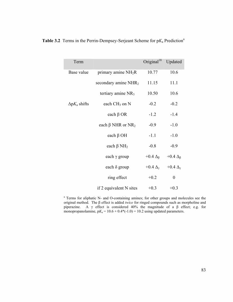
83

Table 3.2 Terms in the Perrin-Dempsey-Serjeant Scheme for pKa Predictiona

Term

Original18 Updated

Base value primary amine NH2R 10.77 10.6

secondary amine NHR2 11.15 11.1

tertiary amine NR3 10.50 10.6

ΔpKa shifts each CH3 on N -0.2 -0.2

each β OR -1.2 -1.4

each β NHR or NR2 -0.9 -1.0

each β OH -1.1 -1.0

each β NH2 -0.8 -0.9

each γ group +0.4 Δβ +0.4 Δβ

each δ group +0.4 Δγ +0.4 Δγ

ring effect +0.2 0

if 2 equivalent N sites +0.3 +0.3

a Terms for aliphatic N- and O-containing amines; for other groups and molecules see the original method. The β effect is added twice for ringed compounds such as morpholine and piperazine. A γ effect is considered 40% the magnitude of a β effect; e.g. for monopropanolamine, pKa = 10.6 + 0.4*(-1.0) = 10.2 using updated parameters.

84

3.2.3 Experimentals

The pKa values of some amines (Table 3.3), outside the training set used for the

development of SHE method and the determination of the updated PDS parameters, were

measured at 25°C to further assess these predictive methods. The potentiometric

titration method developed by Albert and Serjeant was followed (Appendix A). The pKa

values of MEA and MDEA were measured to validate the method.

Table 3.3 Amines Used in Measurement of pKa

Amine CAS # Purity

3-(methylamino)-1,2-propanediol 40137-22-2 ≥98.0%

3-(dimethylamino)-1,2-propanediol 623-57-4 98%

3-(diethylamino)-1,2-propanediol 621-56-7 98%

1,3 Bis(dimethylamino)-2-propanol 5966-51-8 97%

2-{[2-

(dimethylamino)ethyl]methylamino}ethanol] 2212-32-0 98%

Ethanolamine 141-43-5 ≥99.5%

N-methyl-diethanolamine 105-59-9 ≥99%

85

3.3 CONTINUUM-SOLVATION ISSUES

3.3.1 Choice of radii

The accuracy of continuum-solvation computational methods is, unfortunately,

very sensitive to the atomic radii used to define the solute cavity,24,25 and we noted that

the default radii choice changed (from unscaled “UA0” to “UFF” scaled by 1.1) when

Gaussian upgraded its software from G03 to G09. In Figure 3.1, the change shifts pKa

predictions down by an alarming amount: 3-4 units. (There was also a technical change

in cavity and solute-solvent-surface construction in going from G03 to G09 which may

have had a small effect upon predicted pKa.26,27) In Figure 3.1, good estimates for trans

conformers of all acyclic amines (NH3 to DEA) were achieved with the unscaled UA0

radii, and hence this choice was incorporated into the SHE procedure.

Although the UA0 choice provides the highest pKa estimates of the choices in

Figure 3.1, it provides only moderate total molecular volumes (Figure 3.2); the key

seems to be in the volume given to the reactive site, particularly primary and secondary

N atoms, where the UA0 choice results in the smallest volumes (23 and 19 Å3,

respectively; the other procedures use volumes ≥ 26 and 21 Å3, respectively).28

86

Figure 3.1 SHE results without empirical corrections (on conformers of ref. 7), showing

dramatic effects of cavity radii. Dashed line: experiment. Solid squares:

G03 (UA0). Open squares: G09 radii=UA0(x1.1). Solid triangles: G03

radii=UFF. Open triangles: G09 (UFFx1.1). Parentheses denote default

effects.

Figure 3.2 Cavity volumes of B·HOH complexes. See Figure 3.1 for legend.

5

6

7

8

9

10

11

12

13

NH

3

MeN

H2

Me2

NH

Me3

N

ME

A

MIP

A

MP

A

AM

P

AE

EA

DE

A

MO

R

PP

Z

2-M

ePP

Z

1-E

tPP

Z

1-M

ePP

Z

1-(E

tOH

)PP

Z

1,4-

Me2

PP

Z

pKa

87

Regardless of choice of algorithm and radii, there are class-dependent errors

evident in Figure 3.1, particularly the unique errors for cyclic compounds (morpholine

and the piperazines in our case) that have been seen before.7,29 Friesner and co-workers

hypothesized29 that the error shift for cyclic compounds is due to neglecting the 4th type

of non-electrostatic effect: a solvent-structuring effect. Such solvent-structuring may be

clathrate-like;30 solid clathrate structures are known to be stable around cyclic ethers for

example.31 This necessitated the use of separate values for the empirical shift C for

cyclic vs. acyclic amines (discussed in Sec. 3.2.1).

3.3.2 Choice of conformer

An additional unresolved issue is the choice of molecular conformer. This

commonly ignored problem is important because pKa results for alkanolamines are

heavily dependent upon conformer choice (Table 3.4).32 In the examples in the table,

conformer effects are ~0.5 for ethyl group rotation, but they are 2-4 for alkanolamine

internal rotation. The large effect for alkanolamines is due to gauche XCCY

conformations which place the polar X and Y groups in close proximity; this

preferentially stabilizes the BH+ cation in a continnum-solvation calculation, and shifts

up the pKa prediction roughly 2 units per polar gauche interaction.

Note that these large pKa variations with internal rotation of an XCCY unit are as

large as the variations in switching default cavity radii in Figure 3.1. In fact, if G09

default radii (UFF x 1.1) are used, Table 3.4 reveals that one gets the best agreement

with experiment if gauche conformers are used instead of trans ones!

88

We chose the trans + UA0 combination over the gauche + UFFx1.1 combination

mainly because UFF radii show less uniform errors than UA0 radii in Figure 3.1, which

translates into worse rms errors as one tests more amines. It would have been better, of

course, to choose the conformer based on which conformer dominates in aqueous

solutions. Unfortunately, theory has been unable to predict this to date: (i) the rule of

thumb that one should use the lowest-energy conformer in a conformer search cannot be

employed, because although gas-phase and dielectric-continuum optimizations both

predict the gauche forms of both B and BH+ to be lower in energy than the trans forms,

this prediction neglects the effects of explicit hydrogen bonding with solvating water

molecules;34 (ii) two nanosecond-scale classical dynamics simulations of aqueous

monoethanolamine (MEA) which purported to demonstrate preference for gauche

forms35,36 likely did not achieve full equilibration, since bizarrely asymmetric

distributions of observed NCCO dihedral angles were reported in a third such study.37 To

our knowledge the best relevant experimental study of this issue is a 1975 Raman

spectrum study38 which demonstrated that both conformers of neutral MEA are present

in solution; this calls into question the habit of choosing only one for quantum chemistry

computation.

89

Table 3.4 pKa Results from Uncorrected SHE Procedure: Conformer Dependence

Aminea Conformerb pKa G03c pKa G09c

AMP G 11.3 7.9 9.68 T 9.8 6.1

DEA GtgG 12.4 9.3 8.88 GttG 11.9 8.9

TtgG 11.2 7.6 TgtG 10.8 7.4 TttG 10.8 7.3 TggT 9.6 5.8 TgtT 9.5 5.7 TttT 9.5 5.7

DIPA GttG 12.5 9.1 8.84 TttG 10.5 7.3

TttT 8.6 5.3

MEA G 11.7 8.2 9.5 T 10.0 6.3

Et2NH GG 12.2 9.4 10.84 TG 12.1 9.1

TT 11.9 8.9

PPZ GG 12.5 9.2 9.73 TT ax/eq 12.1 8.5

TT ax/ax 12.1 8.5 TT eq/eq 11.7 8.0

TT eq/ax 11.6 7.9

rms error 0.9 1.1 a Experimental pKa values are listed: from Hamborg and Versteeg33 for AMP, DEA, DIPA, and from CRC Handbook23 for MEA, Et2NH, and piperazine. b Gauche and trans descriptors for NCCX dihedrals (G, T) and CNCC dihedrals (g,t) along the main atom chain. The HOCC and PNCC (P = lone pair) dihedrals are not specified in this notation; for T cases we took them to be trans, but for G cases they were chosen to arbitrarily maximize NH…O hydrogen-bond interaction. For PPZ, the axial and equatorial descriptors are for the protonating and spectator N atoms, respectively. c Bold values represent the best single-conformer predictions; the difference between G03 and G09 calculations is the default cavity radii used (UA0 and UFFx1.1, respectively).

90

Table 3.5 Optimized Structures of Geometries of Amines in Table 3.4

Amine/Conformer Neutral Cation

AMP G

AMP T

DEA GtgG

DEA GttG

DEA TtgG

91

Table 3.5 Optimized Structures of Geometries of Amines in Table 3.4 (Continued)


DEA TgtG

DEA TttG

DEA TggT

DEA TgtT

DEA TttT

92



DIPA GttG

DIPA TttG

DIPA TttT

MEA G

MEA T

93



Et2NH gg

Et2NH tg

Et2NH tt

94



PPZ GG (twist-boat)

PPZ TT (chair) ax/eq

PPZ TT (chair) ax/ax

PPZ TT (chair) eq/eq

PPZ TT (chair) eq/ax

95

3.4 RESULTS

If one accepts the limitations inherent in a simple one-conformer procedure with

a traditional continuum-plus-correction methodology, the SHE method constitutes an

improvement within its class, as supported by a direct comparison of SHE results to

those of other continuum-solvation procedures (Table 3.6).

Table 3.6 pKa Results: Comparison of Continuum-Solvation Procedures

a Ref. 23. b Ref. 12. c Ref. 22. d,e Ref. 11 Table 3 “bare” and “H2O”, resp. f,g Ref. 10 Table 2 “pKa calc” and “pKa corrected”, resp.

COSMO JaguarCOSMO-

RSCOSMO-

RSCOSMO-

RSCOSMO-

RS

Amine Expt. a SHE 2010 b 2002 c 2010-1 d 2010-2 e 2006-1 f 2006-2 g

Methylamine 10.66 10.52 10.52 10.5 11.97 11.09 11.71 11.71Dimethylamine 10.73 10.74 10.71 10.9 10.94 9.64 10.67 11.67Trimethylamine 9.8 9.66 10.12 10.1 8.93 7.73 8.63 10.63

MEA 9.5 9.32 9.8 10.29 10.29Morpholine 8.5 8.25 9.5 8.36 9.36rms error 0.2 0.2 0.5 0.9 1.4 0.8 0.9

96

However, SHE is outperformed by the “New PDS” method. Table 3.7 presents

PDS and SHE results for the 32-amine training set. Both SHE and the “New PDS”

methods were trained on this set, and give rms errors of 0.28 and 0.18, respectively. The

optimized structures are given in Table 3.8 and the details of the computation of pKa by

PDS method from group contributions is illustrated in Table 3.9.

97

Table 3.7 SHE vs. PDS Predictions for pKa of 32 Amines

Amine Amine label SHE0a SHE Old PDS

New PDS

Expt. Ref. b

NH(C2H5)2 diethylamine 11.88 11.18 11.15 11.10 10.84 23

NH2(CH2)4NH2 1,4-

butanediamine 11.42 10.72 10.94 10.76 10.80 23

NH(CH3)2 dimethylamine 11.39 10.69 10.75 10.70 10.73 23 N(C2H5)3 triethylamine 11.78 11.08 10.50 10.60 10.75 23

NH2C(CH3)3 tert-butylamine 10.90 10.20 10.77 10.60 10.68 23 NH2CH2CH3 ethylamine 11.28 10.58 10.77 10.60 10.65 23

NH2CH(CH3)2 iso-propylamine 11.13 10.43 10.77 10.60 10.63 23 NH2CH2CH2CH2CH3 butylamine 11.48 10.78 10.77 10.60 10.56 23

NH2CH2CH2CH3 propylamine 11.39 10.69 10.77 10.60 10.54 23

NH2(CH2)3NH2 1,3-

propanediamine 11.34 10.64 10.75 10.54 10.55 23

NH2CH3 methylamine 11.17 10.47 10.57 10.40 10.66 23 NH2CH2CH2CH2OH MPA 10.90 10.20 10.33 10.20 9.96 42

N(CH3)3 trimethylamine 10.31 9.61 9.90 10.00 9.80 23

NH2(CH2)2NH2 1,2-

ethanediamine 10.99 10.29 10.27 10.00 9.92 23

NH(CH3)CH2CH2OH MMEA 10.75 10.05 9.85 9.90 9.85 33 N(C2H5)2CH2CH2OH DEMEA 10.66 9.96 9.40 9.60 9.75 33 NH2C(CH3)2CH2OH AMP 9.76 9.06 9.67 9.60 9.68 33

NH2CH2CH2OH MEA 9.97 9.27 9.67 9.60 9.50 23 NH2CH2CH(CH3)OH MIPA 9.76 9.06 9.67 9.60 9.45 33 N(CH3)2CH2CH2OH DMMEA 9.76 9.06 9.00 9.20 9.22 33 NH(CH2CH2OH)2 DEA 9.47 8.77 8.95 9.10 8.88 41

N(CH3)(CH2CH2OH)2 MDEA 8.64 7.94 8.10 8.40 8.56 40 N(CH2CH2OH)3 TEA 8.53 7.83 7.20 7.60 7.78 23

HN(CH2CH2)2NH PPZ (piperazine) 11.69 9.99 9.85 9.40 9.73 23

C4H9N2(CH3) 2-MePPZ (H+

on 4) 11.60 9.90 9.55 9.10 9.57 39

C4H9N2(C2H5) 1-EtPPZ 11.12 9.42 9.55 9.10 9.20 39 C4H9N2(CH3) 1-MePPZ 11.17 9.47 9.55 9.10 9.14 39

C4H9N2(C2H4OH) 1-(2-EtOH)PPZ 10.96 9.26 9.55 9.10 9.09 39 C4H8N2(CH3)2 1,4-Me2PPZ 9.94 8.24 9.00 8.70 8.38 39

HN(CH2CH2)2O MOR

(morpholine) 9.95 8.25 8.95 8.30 8.50 23

C2H5N(CH2CH2)2O 4-EtMOR 9.16 7.46 8.30 7.80 7.67 23 CH3N(CH2CH2)2O 4-MeMOR 8.76 7.06 8.10 7.60 7.38 23

rms error 1.11 0.28 0.33 0.18 a SHE procedure without empirical corrections C in eq. 3. b Reference for experimental value. Optimized structures are given in Table 3.8.

98


Amine Neutral Cation

1.

diethylamine

2.

1,4-

butanediamine

3.

dimethylamine

4.

triethylamine

5.

tert-butylamine

99



6.

ethylamine

7.

iso-propylamine

8.

butylamine

9.

propylamine

10.

1,3-

propanediamine

100



11.

methylamine

12.

MPA

13

trimethylamine

14.

1,2-ethanediamine

15.

MMEA

101



16.

DEMEA

17.

AMP

18.

MEA

19.

MIPA

20.

DMMEA

102



21.

DEA

22.

MDEA

23.

TEA

24.

PPZ

103



25.

2-MePPZ

26.

1-EtPPZ

27.

1-MePPZ

28.

1-(2-EtOH)PPZ

29.

1,4-Me2PPZ

104



30.

MOR

(morpholine)

31.

4-EtMOR

32. 4-

MeMOR

105

Table 3.9 Group Contributions in Old PDS Predictions for pKa of Amines in Table 3.7

Amine label Old PDS Base Ring N-Me Stat β γ δ

diethylamine 11.15 11.15 0 0 0 0 0 0

1,4-butanediamine 10.94 10.77 0 0 0.3 0 0 -0.13

dimethylamine 10.75 11.15 0 -0.4 0 0 0 0

triethylamine 10.5 10.5 0 0 0 0 0 0

tert-butylamine 10.77 10.77 0 0 0 0 0 0

ethylamine 10.77 10.77 0 0 0 0 0 0

iso-propylamine 10.77 10.77 0 0 0 0 0 0

butylamine 10.77 10.77 0 0 0 0 0 0

propylamine 10.77 10.77 0 0 0 0 0 0

1,3-propanediamine 10.75 10.77 0 0 0.3 0 -0.32 0

methylamine 10.57 10.77 0 -0.2 0 0 0 0

MPA 10.33 10.77 0 0.0 0 0.0 -0.44 0

trimethylamine 9.9 10.5 0 -0.6 0 0 0 0

1,2-ethanediamine 10.27 10.77 0 0 0.3 -0.8 0 0

MMEA 9.85 11.15 0 -0.2 0 -1.1 0 0

DEMEA 9.4 10.50 0 0 0 -1.1 0 0

AMP 9.67 10.77 0 0 0 -1.1 0 0

MEA 9.67 10.77 0 0 0 -1.1 0 0

MIPA 9.67 10.77 0 0 0 -1.1 0 0

DMMEA 9 10.50 0 -0.4 0 -1.1 0 0

DEA 8.95 11.15 0 0 0 -2.2 0 0

MDEA 8.1 10.50 0 -0.2 0 -2.2 0 0

TEA 7.2 10.50 0 0 0 -3.3 0 0

PPZ (piperazine) 9.85 11.15 0.2 0 0 -1.8 0 0

2-MePPZ (H+ on 4) 9.55 11.15 0.2 0 0 -1.8 0 0

1-EtPPZ 9.55 11.15 0.2 0 0 -1.8 0 0

1-MePPZ 9.55 11.15 0.2 0 0 -1.8 0 0

1-(2-EtOH)PPZ 9.55 11.15 0.2 0 0 -1.8 0 0

1,4-Me2PPZ 9 10.50 0.2 -0.4 0 -1.8 0 0

MOR (morpholine) 8.95 11.15 0.2 0 0 -2.4 0 0

4-EtMOR 8.3 10.50 0.2 0 0 -2.4 0 0

4-MeMOR 8.1 10.5 0.2 -0.2 0 -2.4 0 0

106

Table 3.10 presents further comparisons of SHE and New PDS results, for 16

amines outside of the training set, and while the New PDS method is still performing

very well, the SHE method shows further weaknesses, particularly with piperidine and

N-methylpyrrolidine. Looking more closely, the SHE0 calculation (without empirical

shifts) reveals an error that is dependent on class of ringed compound: +1.9 for

piperazines, +1.4 for morpholines, +1.2 for piperidines, and +0.8 for pyrrolidines. It

seems that the entropy change of the surrounding water upon protonation of the amine

(the only term not in the calculation) is important in an ab initio calculation of pKa for

ringed compounds. Rather than introducing more empirical shifts onto a continuum-

solvation electronic structure procedure, one should turn to a simpler procedure that has

only empirical shifts and abandons the electronic structure calculation altogether, i.e. the

empirical PDS methods.

107

Table 3.10 pKa Errors in SHE vs. PDS Predictions Outside the Training Set

Amine pKa(Expt) Ref.a SHE

error

Old

PDS

error

New

PDS

error

piperidine 11.12 23 -0.49 0.23 -0.02 N-methylpyrrolidine 10.46 23 -0.88 0.04 -0.06

cis-2,5-dimethylpiperazine 9.66 23 0.09 0.19 -0.26 2-methoxyethylamine 9.4 23 -0.57 0.17 -0.2 2-(ethylamino)ethanol 9.99 13 -0.01 0.06 0.11 2-(proylamino)ethanol 9.9 13 0.18 0.15 0.2 2-(butylamino)ethanol 9.92 13 0.26 0.13 0.18

pentylamine 10.63 23 0.18 0.14 -0.03 hexylamine 10.56 23 0.27 0.21 0.04

diethylmethylamine 10.35 23 -0.05 -0.05 0.05 3-methyl-1-butylamine 10.6 23 0.27 -0.1 0

3-(methylamino)-1,2-propanediol 9.65 This work

0.12 -0.24 -0.15

3-(dimethylamino)-1,2-propanediol 9.04 This work

0.25 -0.48 -0.24

3-(diethylamino)-1,2-propanediol 9.76 This work

0.07 -0.80 -0.56

1,3 Bis(dimethylamino)-2-propanol 9.41 This work

0.06 -0.55 -0.31

2-{[2-dimethylamino)ethyl]methylamino}ethanol

9.04 This work

-0.54 0.16 0.46

0.35 0.31 0.24 a Reference for experimental value. Optimized structures are given in Table 3.11.

108



piperidine

1-methylpyrrolidine

cis-2,5-

dimethylpiperazine

2-methoxyethylamine

2-(ethylalmino)ethanol

2-(propylamino)ethanol

109

Table 3.11 Optimized Structures of Geometries of Amines in Table 3.10(continued)


2-(butylamino)ethanol

pentylamine

hexylamine

diethylmethylamine

3-methyl-1-

butylamine

110

Table 3.11 Optimized Structures of Geometries of Amines in Table 3.10 (continued)


3-(methylamino)-

1,2-propanediol

3-(dimethylamino)-1,2-propanediol

3-(diethylamino)-1,2-propanediol

1,3 Bis(dimethylamino)-2-propanol

2-{[2-

(dimethylamino)ethyl]methylamino}

ethanol

111

3.4 CONCLUSIONS

For predicting aqueous pKa values of CO2-relevant amines, we have pushed the

continuum-plus-correction method about as far as we can push it, producing a method

(SHE) whose pKa predictions have a root-mean-square error of 0.28 for 32 such amines.

This appears to be an improvement over all other known computer-based methods.

However, the method employs 2 empirical corrections, which would need to be

expanded to accommodate other classes of ringed compounds. The 30-year-old

computer-free group-additivity-based scheme by Perrin, Dempsey, and Serjeant (PDS)

produced an rms error of 0.33 for the same amine set, and with updated parameter values

it produced an rms error of only 0.18. The updated PDS method outperforms the best

continuum-solvation methods in both speed and accuracy, can extend to other ringed

amines, and has no conformer or cavity-radii issues, and hence should be the method of

choice for aliphatic amines. Future work should aim at updating the values of other PDS

parameters for application to other bases and to acids.

112

3.5 REFERENCES

1. Versteeg, G. F.; van Dijck, L. A. J.; van Swaaij, W. P. M. On the Kinetics

Between CO2 and Alkanolamines Both in Aqueous and Non-Aqueous Solutions.


2. da Silva, E. F.; Svendsen, H. F. Prediction of the pKa Values of Amines Using ab

Initio Methods and Free-Energy Perturbations. Ind. Eng. Chem. Res. 2003, 42,

4414.

3. Alongi, K. S.; Shields, G. C. Theoretical Calculations of Acid Dissociation

constants: A Review Article. Ann. Rep. Comput. Chem. 2010, 6, 113.

4. Ho, J.; Coote, M. L. A Universal Approach for Continuum Solvent pKa

Calculations: Are We There Yet? Theor. Chem. Acc. 2010, 125, 3.

5. Brown T. N.; Mora-Diez N. Computational Determination of Aqueous pKa

Values of Protonated Benzimidazoles (Part 1). J. Phys. Chem. B 2006, 110,

9270.

6. Lu H.; Chen X; Zhan C.-G. First-Principles Calculation of pKa for Cocaine,

Nicotine, Neurotransmitters, and Anilines in Aqueous Solution. J. Phys. Chem.

B 2007, 111, 10599.

7. Khalili, F.; Henni, A.; East, A. L. L. Entropy Contributions in pKa Computation:

Application to Alkanolamines and Piperazines. J. Mol. Struct. THEOCHEM

2009, 916, 1.

8. Bryantsev, V. S.; Diallo, M. S.; Goddard, W. A. pKa Calculations of Aliphatic

Amines, Diamines, and Aminoamides via Density Functional Theory with a

113

Poisson-Boltzmann Continuum Solvent Model. J. Phys. Chem. A 2007, 111,

4422.

9. Ulander, J.; Broo, A. Use of Empirical Correction Terms in Calculating

Ionization constants. Int. J. Quant. Chem. 2005, 105, 866.

10. Eckert F.; Klamt A. Accurate Prediction of Basicity in Aqueous Solution with

COSMO-RS. J. Comput. Chem. 2006, 27, 11.

11. Eckert F.; Diedenhofen M.; Klamt A. Towards First Principles Prediction of pKa

and the Cluster-Continuum Approach. Mol. Phys. 2010, 108, 229.

12. Zhang, S.; Baker, J.; Pulay, P. A Reliable and Efficient First Principles-Based

Method for Predicting pKa Value. 1. Methodology. J. Phys. Chem. A 2010, 114,

425.

13. Yamada, H.; Shimizu, S.; Okabe, H.; Matsuzaki, Y.; Chowdhury, F. A.; Fujioka,

Y. Prediction of the Basicity of Aqueous Amine Solutions and the Species

Distribution in the Amine–H2O–CO2 System Using the COSMO-RS Method.

Ind. Eng. Chem. Res. 2010, 49, 2449.

14. Seybold, P. G. Analysis of the pKas of Aliphatic Amines Using Quantum

Chemical Descriptors. Int. J. Quant. Chem. 2008, 108, 2849.

15. Burger, S. K.; Liu, S.; Ayers, P. W. Practical Calculation of Molecular Acidity

with the Aid of a Reference Molecule. J. Phys. Chem. A 2011, 115, 1293.

16. Gaussian03, Revision E.01, Frisch, M. J.; Trucks, G. W.; Schlegel, H. B.;

Scuseria, G. E.; Robb, M. A.; Cheeseman, J. R.; Montgomery, J. A., Jr.; Vreven,

T.; Kudin, K. N.; Burant, J. C.; Millam, J. M.; Iyengar, S. S.; Tomasi, J.; Barone,

V.; Mennucci, B.; Cossi, M.; Scalmani, G.; Rega, N.; Petersson, G. A.; Nakatsuji,

114

H.; Hada, M.; Ehara, M.; Toyota, K.; Fukuda, R.; Hasegawa, J.; Ishida, M.;

Nakajima, T.; Honda, Y.; Kitao, O.; Nakai, H.; Klene, M.; Li, X.; Knox, J. E.;

Hratchian, H. P.; Cross, J. B.; Adamo, C.; Jaramillo, J.; Gomperts, R.; Stratmann,

R. E.; Yazyev, O.; Austin, A. J.; Cammi, R.; Pomelli, C.; Ochterski, J. W.; Ayala,

P. Y.; Morokuma, K.; Voth, G. A.; Salvador, P.; Dannenberg, J. J.; Zakrzewski,

V. G.; Dapprich, S.; Daniels, A. D.; Strain, M. C.; Farkas, O.; Malick, D. K.;

Rabuck, A. D.; Raghavachari, K.; Foresman, J. B.; Ortiz, J. V.; Cui, Q.; Baboul,

A. G.; Clifford, S.; Cioslowski, J.; Stefanov, B. B.; Liu, G.; Liashenko, A.;

Piskorz, P.; Komaromi, I.; Martin, R. L.; Fox, D. J.; Keith, T.; Al-Laham, M. A.;

Peng, C. Y.; Nanayakkara, A.; Challacombe, M.; Gill, P. M. W.; Johnson, B.;

Chen, W.; Wong, M. W.; Gonzalez, C.; Pople, J. A. Gaussian Inc.: Wallingford,

CT, 2004.

17. Gaussian09, Revision B.01, Frisch, M. J.; Trucks, G. W.; Schlegel, H. B.;

Scuseria, G. E.; Robb, M. A.; Cheeseman, J. R.; Scalmani, G.; Barone, V.;

Mennucci, B.; Petersson, G. A.; Nakatsuji, H.; Caricato, M.; Li, X.; Hratchian, H.

P.; Izmaylov, A. F.; Bloino, J.; Zheng, G.; Sonnenberg, J. L.; Hada, M.; Ehara,

M.; Toyota, K.; Fukuda, R.; Hasegawa, J.; Ishida, M.; Nakajima, T.; Honda, Y.;

Kitao, O.; Nakai, H.; Vreven, T.; Montgomery, Jr., J. A.; Peralta, J. E.; Ogliaro,

F.; Bearpark, M.; Heyd, J. J.; Brothers, E.; Kudin, K. N.; Staroverov, V. N.;

Kobayashi, R.; Normand, J.; Raghavachari, K.; Rendell, A.; Burant, J. C.;

Iyengar, S. S.; Tomasi, J.; Cossi, M.; Rega, N.; Millam, N. J.; Klene, M.; Knox,

J. E.; Cross, J. B.; Bakken, V.; Adamo, C.; Jaramillo, J.; Gomperts, R.;

Stratmann, R. E.; Yazyev, O.; Austin, A. J.; Cammi, R.; Pomelli, C.; Ochterski, J.

115

W.; Martin, R. L.; Morokuma, K.; Zakrzewski, V. G.; Voth, G. A.; Salvador, P.;

Dannenberg, J. J.; Dapprich, S.; Daniels, A. D.; Farkas, Ö.; Foresman, J. B.;

Ortiz, J. V.; Cioslowski, J.; Fox, D. J. Gaussian, Inc., Wallingford CT, 2010.

18. Perrin, D. D.; Dempsey, B.; Serjeant, E. P. pKa Prediction for Organic Acids and

Bases, Chapman and Hall: New York, 1981.

19. A relevant example is Hall, H. K. Correlation of the Base Strengths of Amines. J.

Am. Chem. Soc. 1957, 79, 5441.

20. Tissandier, M. D.; Cowen, K. A.; Feng, W. Y.; Gundlach, E.; Cohen, M. H.;

Earhart, A. D.; Coe, J. V.; Tuttle Jr., T. R. The Proton's Absolute Aqueous

Enthalpy and Gibbs Free Energy of Solvation from Cluster-Ion Solvation Data.

J. Phys. Chem. A 1998, 102, 7787.

21. Ben-Naim, A.; Mazo, R. M. Size Dependence of the Solvation Free Energies of

Large Solutes. J. Phys. Chem. 1993, 97, 10829.

22. Klicic, J. J.; Friesner, R. A.; Liu, S.-Y.; Guida, W. C. Accurate Prediction of

Acidity constants in Aqueous Solution via Density Functional Theory and Self-

Consistent Reaction Field Methods. J. Phys. Chem. A 2002, 106, 1327.

23. W. M. Haynes, ed., CRC Handbook of Chemistry and Physics, 92nd Edition,

CRC Press/Taylor and Francis, Boca Raton, FL, 2011.

24. Sadlej-Sosnowska, N. Calculation of Acidic Dissociation constants in Water:

Solvation Free Energy Terms. Their Accuracy and Impact. Theor. Chem. Acc.

2007, 118, 281.

116

25. Behjatmanesh-Ardakani, R.; Karimi, M. A.; Ebady, A. Cavity Shape Effect on

pKa Prediction of Small Amines. J. Mol. Struc. Theochem 2009, 910, 99.

26. Clemente, F. R., private communication.

27. Scalmani, G.; Frisch, M. Continuous Surface Charge Polarizable Continuum

Models of Solvation. I. General formalism. J. Chem. Phys. 2010, 132, 114110.

28. Atom volumes were determined by a group contribution scheme, fitted to the

total volumes of the 17 bases as calculated by Gaussian’s overlapping-spheres

procedure.

29. Marten, B.; Kim, K.; Cortis, C.; Friesner, R. A.; Murphy, R. B.; Ringnalda, M.

N.; Sitkoff, D.; Honig, B. New Model for Calculation of Solvation Free Energies:

Correction of Self-Consistent Reaction Field Continuum Dielectric Theory for

Short-Range Hydrogen-Bonding Effects. J. Phys. Chem. 1996, 100, 11775.

30. Head-Gordon, T. Is Water Structure around Hydrophobic Groups Clathrate-like?

Proc. Natl. Acad. Sci. USA 1995, 92, 8308.

31. Hawkins, R. E.; Davidson, D. W. Dielectric Relaxation in the Clathrate Hydrates

of Some Cyclic Ethers. J. Phys. Chem. 1966, 70, 1889.

32. Effects of up to 4 pKa units were reported in a continuum-solvation-based

computational study of serotonin: see Pratuangdejkul, J.; Nosoongnoen, W.;

Guérin, G.-A.; Loric, S.; Conti, M.; Launay, J.-M.; Manivet, P. Conformational

Dependence of Serotonin Theoretical pKa Prediction. Chem. Phys. Lett. 2006,

420, 538.

117

33. Hamborg, E. S.; Versteeg, G. F. Dissociation constants and Thermodynamic

Properties of Amines and Alkanolamines from (293 to 353) K. J. Chem. Eng.

Data 2009, 54, 1318.

34. Han, B.; Zhou, C.; Wu, J.; Tempel, D. J.; Cheng, H. Understanding CO2 Capture

Mechanisms in Aqueous Monoethanolamine Via First Principles Simulations. J.

Phys. Chem. Lett. 2011, 2, 522.

35. Lopez-Rendon, R.; Mora, M. A.; Alejandre, J.; Tuckerman, M. E. Molecular

Dynamics Simulations of Aqueous Solutions of Ethanolamines. J. Phys. Chem.

B 2006, 110, 14652.

36. da Silva, E. F.; Kuznetsova, T.; Kvamme, B.; Merz Jr., K. M. Molecular

Dynamics Study of Ethanolamine as a Pure Liquid and in Aqueous Solution. J.

Phys. Chem. B 2007, 111, 3695.

37. Gubskaya, A. V.; Kusalik, P. G. Molecular Dynamics Simulation Study of

Ethylene Glycol, Ethylenediamine, and 2-Aminoethanol. 2. Structure in Aqueous

Solutions. J. Phys. Chem. A 2004, 108, 7165.

38. Omura, Y.; Shimanouchi, T. Raman Spectra and Rotational Isomerism of

Ethylenediammonium and Monoethanolammonium Ions in Aqueous Solutions.

J. Mol. Spectrosc. 1975, 55, 430.

39. Khalili, F.; Henni, A.; East, A. L. L. pKa Values of Some Piperazines at (298,

303, 313, and 323) K. J. Chem. Eng. Data 2009, 54, 2914.

118

40. Hamborg, E. S.; Niederer, J. P. M.; Versteeg, G. F. Dissociation constants and

Thermodynamic Properties of Amino Acids Used in CO2 Absorption from (293

to 353) K. J. Chem. Eng. Data 2007, 52, 2491.

41. Bower, V. E.; Robinson, R. A.; Bates, R. G. Acidic Dissociation constant and

related Thermodynamic Quantities for Diethanolammonium Ion in Water from 0°

to 50 °C. J. Res. Natl. Bur. Stand. 1962, 66A, 71.

42. Schwabe, K.; Graichen, W.; Spiethoff, D. Physicochemical Investigations of

Alkanolamines. Z. Phys. Chem. (Munich) 1959, 20, 68.

119

Chapter 4: Reaction Mechanisms in CO2/Aqueous Amine Systems

_______________________________________________________________________

4.1 INTRODUCTION

Meaningful rate constant data for the important CO2-capture reaction

(4.1)

(B = {H2O, OH-, HXYN},) requires agreement about the rate law used to fit to the

experimental data. Two different but widely used mechanisms (the zwitterion1 and

termolecular2 mechanisms) have resulted in competing formalisms and impede

understanding and a third mechanism (the carbamic acid mechanism), a hypothesis

known to engineers in the 1970s,2 has recently been re-emphasized.4,5 A new and

improved modeling study of reaction (4.1) is needed because of various issues arising

from previous modeling efforts. This chapter reports the results of improved quantum

chemistry studies of this reaction, with hopes of clarifying the reaction mechanism.

4.1.1 Overview of competing mechanisms proposed

Zwitterion mechanism. This two-step mechanism, favored by Versteeg,6,7 was a

simplification by Danckwerts2 of a three-step mechanism originally proposed by

Caplow.1 The mechanism assumes a formation of an intermediate zwitterion which then

undergoes a deprotonation by basic molecules resulting in carbamate ion formation:

120

(4.2)

(4.3)

The mechanism only applies to primary and secondary amines due to the need for an NH

bond in the amine HXYN. Caplow’s original mechanism considered the zwitterion’s NH

group to be hydrogen-bonded to a water molecule, and featured an extra proton-transfer

middle step which allows the intermediate to be either H2O·H+XYNCOO− or

H3O+·XYNCOO−.

Applying the steady-state principle to the intermediate zwitterion in eqs 4.2 and

4.3, one obtains the following expression for the rate of reaction of CO2 ( :

∑

, (4.4)

where (4.5)

Here is the overall reaction rate constant for CO2 loss, and , , and are the

elementary rate constants in steps (2) and (3). B denotes any proton-accepting species

present; if one considers {H2O, OH-, HXYN}, then one has elementary rate constants kB

= {kw, kOH-, and kHXYN} and the corresponding composites KB from eq. (4.5).

Equation (4.4) is very general and can cover aqueous and non-aqueous amine

solutions. Fitting this equation to experimental data for aqueous amines would give

values for the three KB’s as well as , but this 4-parameter function often has

indeterminacy problems. For simplification, Danckwerts2 reiterated Caplow’s two

121

limiting cases (and generalized them to allow for other possibilities of B): simplifications

arise if k-1 << ∑ (eq. 4.6) or k-1 >> ∑ (eq. 4.7).

(4.6)

(4.7)

Equation (4.7), like (4.5), allows for fractional orders of amine between 1 and 2.

Termolecular mechanism. In 1990 Crooks and Donnellan3 challenged the belief

in an unobserved carbamate zwitterion intermediate, instead suggesting that overall

reaction (4.1) consists of one elementary termolecular step.4,5 The resulting rate law

matches eq. (4.7) but without the eq. (4.5) interpretation of the KB constants.

Meader and co-workers4,5 have frowned upon this mechanism, using the usual

theoretical argument that a termolecular elementary step requires simultaneous collision

of 3 entities. However, in solutions in which strong hydrogen bonding can occur,

complexes of 2 of the 3 entities pre-exist and this counter-argument is invalid. Crooks

and Donnellan did in fact suggest that the single step starts from an “encounter complex”

that is not zwitterionic. If formation of an encounter complex does not result in loss of

CO2 signal (like zwitterion formation would), the complexation stage would not affect

measured rate of CO2 loss, and hence CO2 loss would be solely due to the ensuing

concerted elementary step involving two bonds forming and two bonds breaking

amongst the three entities. This is what should be inferred from the label “termolecular

mechanism.”

122

Carbamic acid mechanism. Meader and co-workers4,5 favors the two-step

mechanism in which the intermediate is not the zwitterion but hydrogen carbamate

(“carbamic acid”) molecules:

(4.8)

(4.9)

Step (4.8) cannot be elementary on its own due to egregious bond strain that would exist

in a concerted transition state. It might be possible as a termolecular step from a Crooks-

Donnellan encounter complex with H2O or alcohol solvent molecules, in which case, 3

bonds are breaking and forming in a concerted manner.

Bicarbonate mechanisms. Equation (4.1) (carbamate formation) is not the only

CO2-capture reaction possible in amine solutions. It is known that ordinary basic

solutions can convert CO2 to bicarbonate in small amounts:

(4.10)

or (4.11)

Eq. (4.11), a base-catalyzed bicarbonate mechanism proposed by Donaldson and

Nguyen,8 is believed to be operative in the case of tertiary amines, which cannot form

carbamates. This base-catalyzed bicarbonate mechanism is, like the Crooks-Donaldson

base-catalyzed carbamate mechanism, a “termoleculecular” single-step mechanism, in

which two bonds are broken and two bonds are formed in a concerted step amongst the

three molecular entities within an encounter complex. The rate expression for (4.11) is:

(4.12)

where should be independent of amine concentration.

123

4.1.2 Previous modeling studies

Obtaining realistic mechanistic results using theoretical molecular models depend

on a number of factors – one being the use of a proper molecular model capable of

representing the essential chemistry of the real liquid solution. For liquid phase reactions

involving ions, one important modeling aspect is the stabilization of ions by polar

solvents: polar solvents will lower the energy of ionic intermediates and transition states

dramatically, thus affecting the rate and even course of reactions. A second aspect,

important in the current case of aqueous amines, is the local hydrogen-bonding solvation

effects.

A continuum solvation model (CSM), such as PCM,9 SMx,10 and COSMO,11 can

be used to incorporate most of the first effect. In CSM, the solute molecule or ion is

hypothetically placed in a semiempirically built cavity inside a continuum dielectric

having an adjustable polar strength parameter ε. Unfortunately, the use of a CSM does

not provide the effects of hydrogen bonding. Use of explicit solvent molecules in the

modeling (with or without CSM) is a common way of incorporating this second effect.

Previous computational chemistry studies of equation (1) have tried both of these

modeling strategies, but the results reveal problems which my work aims to address.

These problems are now discussed.

Non-observance of carbamate in single-amine modeling: It has been known

since 1925 that the dominant initial product upon reacting CO2 with aqueous amines is

carbamate ion12. To date, however, single-amine models (regardless of their use of CSM

124

or explicit water molecules) have been unable to produce carbamate as intermediates at

all (summarized in Table 4.1).

Table 4.1 Reaction Pathways Observed in Single-Amine Modeling

Reference Level of modeling

Results

13 (Arstad et al., 2007)

Gas phase with explicit water

CO2+MEA+H2O carbamic acid CO2+DEA+H2O carbamic acid

14 (Shim et al., 2009) IEFPCM CO2+MEA+H2O zwitterion

15 (Xie et al., 2010) CPCM CO2+MEA+H2Ozwitterion carbamic acid

16 (Han et al., 2011) COSMO CO2+MEA+H2O carbamic acid

17 (Ismael et al., 2009)

COSMO CO2+AMP+H2O carbamic acid

18 (Yamada et al., 2011)

IEFPCM-SMD CO2+AMP+H2O zwitterion carbamic acid

Altogether, the most common product in Table 4.1 is carbamic acid. We

speculated that more explicit water might properly stabilize the anionic product and we

will show that we were correct.

Disagreement on intermediate energies in double-amine modeling. Previous

two-amine-molecule studies (summarized in Table 4.2) have succeeded in finding

carbamate ions as intermediates, likely because these studies mimic very basic pH

conditions. These studies also generally observe zwitterion intermediates, but disagree

on the relative stability of zwitterion vs. carbamate ion.

125

Table 4.2 Reaction Pathways Observed in Double-Amine Modeling

Reference Level of modeling

Results

13 (Arstad et al., 2007)

Gas phase with explicit water

CO2+2MEA carbamic acid and CO2+2MEA carbamate

14 (Shim et al., 2009) IEFPCM CO2+2MEA carbamate

15 (Xie et al., 2010) CPCM MEA+MEA-zwitterioncarbamate

16 (Han et al., 2011) COSMO MEA+MEA-zwitterioncarbamate

18 (Yamada et al., 2011)

IEF-PCM-SMD MEA+AMP-zwitterioncarbamate

Shim et al. (2009)14 found a one-step mechanism with crude coordinate scanning,

which made them conclude that the overall reaction (CO2+2MEA) was termolecular,

although they stressed that a more concrete conclusion regarding zwitterion stability

warrants further consideration of solvation effect through explicit water molecules.

However, three later papers15,16,17 used proper transition state search and found a step

from zwitterion to carbamate ion. Puzzlingly, they disagree on the exothermicity of this

step. Again, we speculated that more explicit H2O in the modeling would help, and

properly show the consecutive exothermic steps.

126

Role of catalyst in two-amine modeling. Due to the non-observance of carbamate

in single-amine modeling, Shim et al. (2009)14 undermined the role of water as base, and

then emphasized its catalytic role in proton relay in two-amine modeling. They

hypothesized a quadrumolecular mechanism where a water molecule assists in amine-to-

amine proton-transfer. However, their hypothesized mechanistic pathway has not

received attention in subsequent studies. On the other hand, the catalytic role of amine in

two-amine modeling was emphasized by Arstad et al. (2007).13 They studied formation

of both carbamate and carbamic acid in separate pathways from (CO2+2MEA), and

thought that the amine-catalyzed ‘carbamic acid’ formation pathway was the most

plausible mechanism as it gave reaction order 1 with respect to MEA and had the right

activation energy. However, this has not been properly studied using a CSM. We will

study these mechanistic pathways at the same level of modeling as in other mechanisms.

Carbamic acid equilibria. None of the previous studies discuss the possible pH-

dependent equilibrium between “carbamic acid”/carbamate/zwitterion, relevant to the

carbamic acid hypothesis (eqs. 4.8 and 4.9).

Origin of activation energy barrier. da Silva et al. (2004)19 hypothesized that the

reaction barrier for CO2 absorption in aqueous monoethanol amine solution is caused by

the displacement of water molecules in the solvation shell of the amine group as CO2

approaches. The potential of mean force (PMF) calculations of Xie et al. (2010)15 also

suggest there is a small barrier due to solvent displacement in the formation of

zwitterion. However, PCM calculations published so far14-18 did not consider the solvent

displacement and hence drew different conclusions. We will study the reaction of CO2

with an amine which is N-HO and/or H-OH hydrogen-bonded with water (or N-HN

127

and/or NH-N hydrogen-bonded with other amine) using PCM calculations to see if a

transition state involving H2O displacement can be found.

Effect of pKa on mechanism. None of the previous studies have investigated the

effects of the basicity of the amine upon mechanism.

Thus, we still lack a good modeling study that can address the three hypotheses

for the mechanism of the CO2-capture reaction. In this work, a semi-continuum CSM-

plus-explicit-water model is used, addressing Shim et al.’s call for more explicit water

molecules in the modeling by adding as many as twenty in some instances. It will be

shown that such consideration will have important consequences in many aspects of the

reaction: for example, observance and relative stability of intermediates, activation

energies depending on degree of solvation of transition states or reactants, reaction

energy barrier due to solvent displacement, complexity in modeling bicarbonate

formation, and basicity (pKa) effects.

128

4.2 METHOD

In the pKa study (Chapter 3), hydrogen bonding was treated in a semi-continuum

manner: by including an explicit water molecule forming a hydrogen bond with the

neutral amine and protonated amine. Here, in studying the mechanistic pathway of

reaction of CO2 in aqueous alkanolamine, the same technique is used, since the cation,

anion, zwitterion, and neutrals are all capable of forming hydrogen bonds.

All calculations were done using the Gaussian0920 computational chemistry

software program on in-house supercomputer Dextrose. The electronic structure

approximation used was a density functional theory (DFT): the B3LYP 21,22 functional

combination, with the 6-31G(d) basis set for molecular orbital construction. The

polarization effect of solvation was modeled using a polarizable continuum model

(PCM), with UFF atomic radii used for overlapping-sphere solute cavity construction

within the continuum (algorithm: scrf=IEFPCM; solvent=water).23 Energies are

generally reported “raw” without zero-point and thermal-correction energies.

Full molecule geometry optimizations were performed. For determining

activation energies, the algorithm opt=(ts, calcfc, noeigentest)24 was used for transition

state (TS) optimization. Transition states were confirmed by vibrational frequency

computation (freq=noraman; one imaginary frequency needed) and by two energy

minimization runs, each starting from the TS geometry but with some atoms displaced

according to the direction shown in the imaginary-frequency normal mode.

129

Most results employ methylamine (MeNH2) or monoethanolamine (MEA) as the

amine HXYZ, with varying numbers of explicit H2O molecules in a hydrogen-bonded

cluster.

4.3 RESULTS AND DISCUSSION

This section is organized as follows. Demonstration of the need for many explicit

water molecules to determine the dominant intermediate occurs in section 4.3.1. This is

followed by reaction pathways originating from single-MEA modeling

(CO2+MEA+nH2O) and double-MEA modeling (CO2+2MEA+nH2O) in sections 4.3.2

and 4.3.3, with a cross comparison in section 4.3.4. The alternative bicarbonate-

formation pathways, and the effects of varying pKa (i.e. choosing other amines) on

reaction mechanisms, are discussed in sections 4.3.5 and 4.3.6 respectively.

4.3.1 Effect of spectator water molecules on ion solvation

The main problem with previous computational modeling of the CO2 + amine

reaction has been the peculiar non-observance of the well-known carbamate anion

product. To investigate why, a series of computations were performed, using

methylamine as a test amine, to determine the exothermicity of the carbamate-

producing reactions R1-R4 as functions of the number of water molecules explicitly

used to solvate the solute species. R1 and R3 form carbamate ions from the zwitterion,

whereas R2 and R4 form carbamate ions from carbamic acid molecules.

130

Single amine (neutral pH) model:

MeNH2COO·(n H2O) + H2O·(n H2O) MeNHCOO−·(n H2O) + H3O+·(n H2O)

(R1)

MeNHCOOH·(n H2O) + H2O·(n H2O) MeNHCOO−·(n H2O)) + H3O+·(n H2O)

(R2)

Double-amine (very basic pH) model:

MeNH2COO·(n H2O) + MeNH2·(n H2O) MeNHCOO−·(n H2O) + MeNH3+·(n H2O)

(R3)

MeNHCOOH·(n H2O) + MeNH2·(n H2O) MeNHCOO−·(n H2O) + MeNH3+·(n H2O)

(R4)

The B3LYP/6-31G(d)/UFF-PCM level of theory was used, and lowest-energy

conformers (Figure 4.1) were located from multiple trials. The raw ΔE results for these

reactions are graphically shown in Figure 4.2. As the number of explicit water

molecules was increased, a large lowering of ΔE was seen in Figure 4.2 for all four

reactions, due to improved solvation of the two created ions. Without explicit waters,

one would mistakenly conclude that the thermodynamically favored species in the

carbamate equilibria is either zwitterion or carbamic acid molecules. Thus, the peculiar

non-observance of carbamate anions in previously published work is due to improper

omission of explicit H2O molecules in the models.

Upon proper addition of explicit waters, Figure 4.2 reveals that the carbamate

anion becomes competitive at neutral pH (R1, R2), and dominant at basic pH (R3, R4).

This brings the modeling results into agreement with experimental observations,25 that

carbamates are quite unstable at neutral pH, but stable for hours in basic solution.

131

Figure 4.1 Conformers of X·(n H2O) complexes used in section 4.3.1 (B3LYP/6-

31G(d)/UFF-PCM).

n=0 n=1 n=2 n=3

Zwitterion

MeNH2COO

Carbamate

MeNHCOO−

Carbamic

Acid

MeNHCOOH

MeNH2

MeNH3+

H2O

H3O+

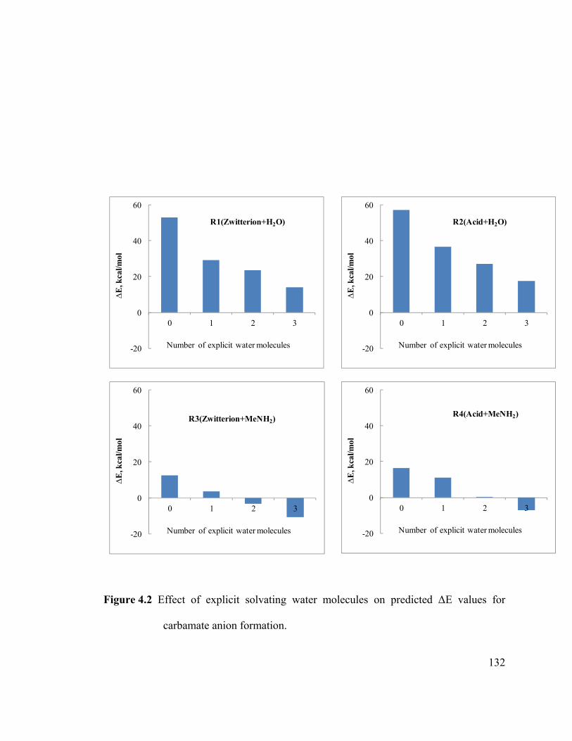
132

Figure 4.2 Effect of explicit solvating water molecules on predicted ΔE values for

carbamate anion formation.

-20

0

20

40

60

0 1 2 3

∆E

, kca

l/mol

Number of explicit water molecules

R1(Zwitterion+H2O)

-20

0

20

40

60

0 1 2 3

∆E

, kca

l/mol


R2(Acid+H2O)

-20

0

20

40

60

0 1 2 3

∆E

, kca

l/mol


R3(Zwitterion+MeNH2)

-20

0

20

40

60

0 1 2 3

∆E

, kca

l/mol


R4(Acid+MeNH2)

133

4.3.2 Carbamate formation at neutral pH

The mechanistic pathway for the formation and breakdown of carbamate at

neutral pH (single-amine modeling) will be explored in this section, using MEA as the

amine. Results are presented for 1-H2O, 5-H2O and 20-H2O models. The mechanisms

observed appear in Figure 4.3. Clearly, mechanisms incorporating other numbers of

H2O in the proton relay are also possible.

6-atom cycle

(1-H2O modeling)

O C O

N

HR

RH

O

H

H

OH

H

OH

10-atom cycle

(5-H2O modeling)

12-atom cycle

(20-H2O modeling)

Figure 4.3 Reaction mechanisms observed in the modeling of eq (1) with B=H2O.

6-atom cycle. In 1-amine-1-H2O modeling, the 6-atom cycle in Figure 4.3

(involving 2 H transfers) occurred in a 2-step pathway, forming carbamic acid via

zwitterion intermediate. Structures and energies appear in Figure 4.4. This poor level of

134

modeling, employed by others 13-18 results in an overly high barrier between zwitterion

and acid forms, with no carbamate intermediate there.

TS1 reactant

TS1

TS1 product

TS2 reactant

TS2

TS3 product

Figure 4.4 B3LYP/6-31G(d)/UFF-PCM results for 1-amine-1-H2O modeling.

Elementary-step activation energies in parentheses.

-20

-15

-10

-5

0

5

10

15

20

Rel

ativ

e en

ergy

, kca

l/mol

TS1 reactant(Initial complex)

TS1 product/TS2 reactant(Zwitterion)

TS1 (0.94)

TS2(10)

TS2 product(Carbamicacid)

135

10-atom cycle. In 1-amine-5-H2O modeling, the pathway found was a 10-atom

cycle (involving 4 H transfers) occurring in a 3-step pathway. Structure and energies are

shown in Figure 4.5. Here, the first step is again simple zwitterion formation, but it

involves displacement by CO2 of an initial N…H hydrogen bond between amine N and

a water molecule (labeled as H23-O22-H24 in Figure 4.5) and consequently has a

higher activation energy barrier than in Figure 4.4. (Note that da Silva and Svendsen

believed that the activation energy barrier for CO2 capture by MEA arises from water

displacement.) In the second step, the zwitterion here converts not into a carbamic acid

directly, but first into a carbamate intermediate by the abstraction of the proton by

another water molecule (H17-O9-H15) that acts as base in this step. The presence of

additional explicit water molecules has considerably stabilized the creation of two

molecular ions here (the carbamate anion and a hydronium cation). The third step

produces the acid form via more H atom exchanges. So, now we see we have enough

H2O in the model to see a carbamate anion intermediate and a reduction of the overly

high barrier in 1-amine-1-H2O modeling. Unfortunately, this level of modeling is also

poor because of the predicted final step to an excessively stable carbamic acid, a form

which has not been experimentally observed.

136

TS3 reactant

TS3 product (zwitterion)

TS4 reactant (zwitterion)

TS4 product (carbamate)

TS5 reactant (carbamate)

TS5 product (acid)

Figure 4.5 B3LYP/6-31G(d)/UFF-PCM results for 1-amine-5-H2O modeling.

Elementary-step activation energies in parentheses.

-20

-15

-10

-5

0

5

10

15

20

Rel

ativ

e en

ergy

, kca

l/mol

TS3(7.58)

TS4(3.64)

TS4product(Carbamate)

TS3 product(Zwitterion)

TS5reactant(Carbamate)

TS5(0.49)

Carbamicacid

TS3reactnat(Initialcomplex)

TS4 reactant(Zwitterion)

137

12-atom cycle. In 1-amine-20-H2O modeling, the pathway found was a 12-atom

cycle (involving 5 H transfers). The initial step of zwitterion formation was omitted due

to the uncertainty in knowing how many H-bonds to displace in this bimolecular step.

Transition structures and energies for the 2nd and final steps appear in Figure 4.6. With

the H2O molecules now properly surrounding the amino and carboxyl groups, and the

addition of more explicit H2O, the carbamates are now seen to be thermodynamically

competitive with both the zwitterion and carbamic acid forms at the B3LYLP/6-

31G(d)/UFF-PCM level (Figure 4.6). The single-point energy calculations at the

alternative MP2/6-31G(d,p)/UFF-PCM level are presented to point out that the expected

accuracy of B3LYP and MP2 is perhaps 2-4 kcal/mol.

The 1-amine-20-H2O data should be the best to date for neutral-pH modeling. If

the encounter complex has similar raw energy to these intermediates, as suggested by

Figures 4.4 and 4.5, then it would have the lowest free energy of all these forms because

of the entropy benefit of dissociation; this agrees with the fact that carbamate in basic

solutions quickly decomposes to CO2 + amine when brought to pH = 7.25

138

TS6 (proton H57 is being transferred

from N23 to O15)

TS8 ((proton H38 is being

transferred from O8 to.O21)

Figure 4.6 Results for 1-amine-20-H2O modeling. Energy profiles are at B3LYP/6-

31G(d) (square) and at MP2/6-31G(d,p) (triangle) level. Elementary-step

activation energies at the B3LYP/6-31G(d) level in parentheses.

-20

-15

-10

-5

0

5

10

15

20

Rel

ativ

e p

oten

tial

en

ergy

, k

cal/m

ol

Zwitterion

TS6(3.56)

Carbamate Carbamate Acid

TS7(0.01)

TS8(4.46)

139

4.3.3 Carbamate formation at basic pH

In concentrated alkanolamine solutions of basic pH, carbamate ions can be stable

for several hours 25, so the energetics must be different than that of Figure 4.6. Basic pH

systems are better modeled by having two amine molecules in the model; thus, this

section deals with 2-amine-molecule modeling.

Initial modeling without spectator water molecules (B3LYP/6-31G(d)/UFF-PCM

level of theory) produced 3 different atom-cycle possibilities; the observed mechanisms

are summarized in Figure 4.7.

6-atom cycle

5-atom cycle

8-atom cycle

Figure 4.7 Reaction mechanisms observed in the modeling of eq (1) with B=amine.

5 and 6-atom cycle. The 6-atom cycle was first studied. A 2007 gas-phase study

13 predicted a single-step pathway forming carbamic acid products. However, results

here with the PCM continuum solvent shell predict this pathway to be multi-step. With

the usual all-trans conformer of the amine MEA, calculations here predict this pathway

140

to be two-step via zwitterion intermediate (Figure 4.8), just as in our 6-atom cycle in

neutral-pH modeling (Figure 4.4). Out of curiosity, the 6-atom cycle was also

investigated here with a maximally internally H-bonded initial complex, generated by

use of gauche (instead of trans) MEA. This gauche-MEA pathway produced a three-step

mechanism, with carbamate ion as the additional intermediate (Figure 4.9). Figure 4.9

reveals greater activation energy than Figure 4.8 (7 vs. 1 kcal/mol for the first step)

because there are more H-bonds to break to get to the first transition state. In addition, a

5-atom three-step cycle (Figure 4.10) was found by reorienting the all-trans MEA

molecules in Figure. 4.8 in a manner more consistent with the orientation used by

others15,16 for the zwitterion-to-carbamate step. This cycle is a 5-atom cycle because the

H atom donated to the catalytic amine in the second step is the same one that is returned

to the carbamate ion in the third step.

Most importantly, none of these 2-amine-0-H2O modeling results (Figures 4.8-

4.10) show a thermodynamic preference for the carbamate ion as the product, and hence

they do not agree with experiment (Wang et al, 1972).25 There are not enough explicit

H2O molecules in the model to show the expected stability of the carbamate ion.

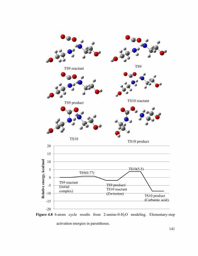
141

TS9 reactant

TS9

TS9 product

TS10 reactant

TS10

TS10 product

Figure 4.8 6-atom cycle results from 2-amine-0-H2O modeling. Elementary-step

activation energies in parentheses.

-20

-15

-10

-5

0

5

10

15

20

Rel

ativ

e en

ergy

, kca

l/mol

TS9 reactant(Initial complex)

TS9 product/TS10 reactant(Zwtterion)

TS9(0.77)TS10(5.5)

TS10 product(Carbamic acid)

142

TS11reactant

TS11

TS12

TS12 product

TS13

TS13 product

Figure 4.9 6-atom cycle results for 2-amine-0-H2O modeling, but with gauche MEA for

maximal H-bonding at the outset. Elementary-step activation energies in

parentheses.

-20

-15

-10

-5

0

5

10

15

20

Rel

ativ

e en

ergy

, kca

l/mol

TS11(InitialComplex)

TS11 (7)

TS13(0.64)

TS12(5.4)

TS11 product(Zwtterion) TS12 product

(Carbamate) TS13 product(Acid)

143

TS14 reactant TS14

TS15

TS15 product

TS16

TS16 product

Figure 4.10 5-atom cycle results from 2-amine-0-H2O modeling. Elementary-step

activation energies in parentheses.

-20

-15

-10

-5

0

5

10

15

20

Rel

ativ

e en

ergy

, kc

al/m

ol

TS14 reactant(InitialComplex)

TS16(3.7)

TS16 reactant(Carbamate)

TS16 product(Acid)

TS15 (5)TS14 (0.77)

TS15 product(Carbamate)TS14 product

(Zwtterion)

144

8-atom cycle. An 8-atom cycle (shown earlier in Figure 4.7, right) was found by

adding one water molecule between the two amines, to test a recent hypothesis (Shim et

al. 2009).14 The resulting structures and PEP of the three-step pathway are shown in

Figure 4.11. Comparison of the energetics here to the corresponding 6-atom cycle

(Figure 4.8) shows that adding an H2O molecule to the relay produced a slightly higher

energy pathway. More importantly, this 2-amine-1-H2O pathway, unlike the 2-amine-0-

H2O pathways of Figures 4.8-4.10, did produce the carbamate ion as the lowest-energy

form along the pathway, but not as an energetically dominant species. More H2O

molecules are probably required, as they were in the neutral-pH modeling of the previous

section.

As an initial check of the benefits of spectator H2O molecules, two were

sequentially added to the TS44 structure of Figure 4.10 and reoptimized, together with

the related reactants (zwitterion) and products (carbamate). The results (Figure 4.12)

show that the elementary reaction energy for this step is lowerd 4 kcal/mol for each of

the two waters added, confirming our suspicion that adding spectator waters would

improve the thermochemistry.

145

TS17 product

TS18

TS18 product

TS19 product

Figure 4.11 8-atom cycle with 2-amine-1-H2O modeling. Elementary-step activation

energies in parentheses.

-20

-15

-10

-5

0

5

10

15

20

Rel

ativ

e en

ergy

, kca

l/mol

TS19 product(Carbamicacid)

TS18(7.24)

TS17(0.72)

TS17 reactant(Initialcomplex) TS18 product

(Carbamate)

TS19(2.9)

TS17 product(Zwitterion)

146

TS15

TS15 product

TS20

TS20 product

TS21

TS21 product

Figure 4.12 Effect of varying n in 2-amine-n-H2O modeling (zwitterion-to-carbamate

step). Elementary-step activation energies in parentheses.

-4

0

4

8

Rel

ativ

e en

ergy

, kc

al/m

ol

No water molecule One water molecule Two water molecules

Carbamate

Zwitterion

Carbamate

Carbamate

TS15(5.06)

TS20(2.75)

TS21(0.99)

147

Finally, a 2-amine-18-H2O model (8-atom cycle) was attempted. Now the

carbamate ion intermediate is correctly predicted to be the thermodynamically dominant

product of reaction (Figures 4.13 and 4.14). Note the negligible activation barrier of

0.16 kcal/mol for its formation from zwitterion; this concurs with conclusions drawn

from lower-level modeling (Xie 2010).15 Extending the proton relay by adding a 19th

H2O between the two amines (as we did in going from Figure 4.8 to Figure 4.11) was

also performed but it increased the activation energy (to 2.1 kcal/mol) as it did before, so

the Figure 4.13 pathway represents the more plausible pathway at basic pH.

148

Figure 4.13 Results from 2-amine-18-H2O modeling. Elementary-step activation

energies in parentheses.

-20

-15

-10

-5

0

5

10

15

20

Rel

ativ

e en

ergy

, kca

l/mol

TS22 product (Carbamate)

TS23(B3LYP=18.7)

TS 22(B3LYP=0.16)

TS22 reactant(Zwitterion)

TS23 product(Carbamic Acid)

TS23 reactant(Carbamate)

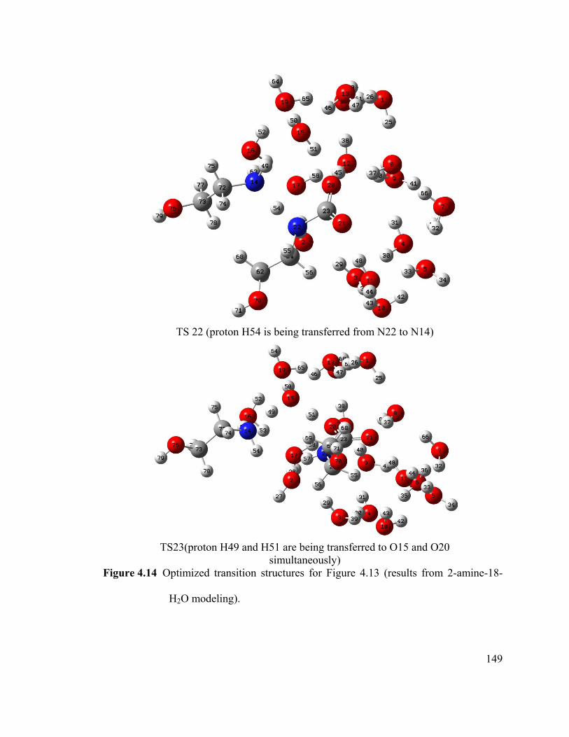
149

TS 22 (proton H54 is being transferred from N22 to N14)

TS23(proton H49 and H51 are being transferred to O15 and O20 simultaneously)

Figure 4.14 Optimized transition structures for Figure 4.13 (results from 2-amine-18-

H2O modeling).

150

4.3.4 Discussion: Formation of carbamate

It is apropos to compare the best results from basic-pH modeling (Figure 4.13) to

those of neutral-pH modeling (Figure 4.6). We focus on the zwitterion-to-carbamate

elementary step, whose exothermicity is significantly enhanced by additional explicit

water molecules in the modeling. The smaller activation barrier in two-amine modeling

vs. one-amine modeling is due to its transition state being “earlier” (Hammond’s

Postulate), which in turn is due to the step being more exothermic (Bell-Evans-Polanyi

Principle). To demonstrate the increasing “earliness” of the TS for this step in 2-amine

modeling, the activation energies from Figures 4.12 and 4.13 are plotted in Figure 4.15

against the N-H bond length of the zwitterion, which increases from 1.1 Å to 1.8 Å

during this step. As more H2O molecules are added (going left to right in the plot), the

increased exothermicity drives down the activation energy (triangle points), which

directly correlates to the transition-state N-H bond length occurring earlier (diamond

points). In fact, the increased exothermicity even impacts the N-H bond length in the

reactant zwitterion, mildly stretching it (square points). The activation energy barrier is

proportional to the vertical distance between the square and triangle points (i.e. to the

amount the N-H distance has to stretch to get to the TS), which shrinks with increasing

solvation of the system. For comparison, at the right side of Figure 4.15, the data from

the single-amine-20-water modeling (“A20”) previously presented in Figure 4.6 is

shown. Comparing A20 to B18 (double-amine-18-water modeling) data, the transition

151

state for A20 modeling is “later” (R (N-H) =1.35 vs. 1.20 Å), correlating with its larger

barrier (3.5 vs. 0.2 kcal/mol) for this exothermic step.

Figure 4.15 Effect of level of modeling on zwitterion deprotonation step

0

2

4

6

8

10

1

1.1

1.2

1.3

1.4

1.5

B0 B1 B2 B18 A20

Act

ivat

ion

en

ergy

(k

cal/m

ol)

N-H

bon

d le

ngt

h(Å

)

Level of modelling denoted by A (single-amine) and B (double-amine) followed by the number of water molecules in the model

N-H distance in TSN-H distance in zwitterionActivation energy

152

Comparison of Figure 4.6 (neutral pH) with Figure 4.13 (basic pH) suggests that

the zwitterion intermediate plays a role in dilute solutions where the amines are

completely solvated with water molecules (and perhaps for the ones Caplow studied,

using ordinary not-so-soluble amines) but would play essentially no role when an NH-N

hydrogen bond is present as might be the case in significantly basic solutions (modern-

day concentrated alkanolamine solutions). Therefore, both Zwitterion and Termolecular

mechanisms are valid mechanisms but the major route for the reactants will depend on

environment (concentration and nature of amines). This also explains that at low

concentration the reaction order in amine will be near unity, but with increasing

concentration, broken order of reaction greater than one will appear (Aboudhier et al.,

2003). Deprotonation by water molecules is statistically possible but would generally

be followed by relaying the proton to another amine so that overall heat of reaction will

be same as in the case of direct deprotonation by amine (Hess’s law). With slightly

more certainty one can say that our results do not support the Carbamic Acid

mechanism, since at the best levels of modeling this intermediate would appear after a

carbamate ion and would not be thermodynamically favored in any equilibrium.

Figure 4.13 suggests that the rate-limiting step for overall CO2 absorption (Eq.

4.1) in concentrated alkanolamine solutions would not be zwitterion deprotonation (in

agreement with Versteeg (Versteeg 1996))6 but rate of encounter of CO2 with an amine

molecule. This step would have an Arrhenius prefactor which would be affected by

things like rate of bubbling CO2 into the mixture, and rate of diffusing CO2 molecules

towards amine molecules within the solution (affected by stirring rate). This step might

also have activation energy, and to gain insight here, attempts were made to compute

153

zwitterion formation steps from encounter complexes within a large-water network. The

activation energies were often disturbingly large (as an example, 19.5 kcal/mol in a 1-

amine-19-H2O case), due to the reduction of total number of hydrogen bonds as CO2

heads towards amine. Since the number of broken H-bonds was dependent on starting

conformation, the quantitative values of the activation energy were dependent on

starting conformation and hence did not warrant presentation here.

154

4.3.5 Formation of bicarbonate

Figure 4.16 Mechanism for bicarbonic acid formation through 6-atom cycle

The bicarbonate-forming CO2 capture mechanism in Eq. 4.11 was also studied, in

hopes of understanding why this mechanism does not compete well with the carbamate-

forming reactions in the cases of primary and secondary amines. First, a 6-atom cycle

through to carbonic acid was studied (Figure 4.16), analogous to the 6-atom cycle

through to carbamic acid (Figure 3) used to study the carbamate-forming pathway. The

two-step energy profile and the optimized geometries are shown in Figure 4.17. The

transition state for the bicarbonate formation is the theoretical “carbonic acid

zwitterion” strongly complexed with the amine. No supporting water molecules were

necessary to observe the bicarbonate, but the activation energy and heat of reaction for

bicarbonate formation are 9.1 and -3.5 kcal/mol, whose magnitudes seem too high and

too low, respectively.

Use of one spectator water molecule to stabilize the CO2 in the transition state

reduced the barrier to 5.8 kcal/mol (TS 26 in Figure 4.17). Various pathways with

large-water network were attempted but the problem with this CO2-to-bicarbonate

reaction is that the important step starts right from the encounter complex, and this

complex is quite dependent on conformer which controls the H-bond differential in this

bimolecular step. Hence, the extension to more H2O caused insurmountable problems

with this reaction.

H

O H

CO

ON

H

R

R

155

TS24 reactant

TS24

TS24 product

TS25 reactant

TS25(activation energy=9.1kcal/mol)

TS25 product

TS26 reactant

TS26 (activation

energy=5.8 kcal/mol)

TS26 product

Figure 4.17 Bicarbonate formation through 1-amine-1-H2O 6-atom cycle.

-20

-15

-10

-5

0

5

10

15

20

Rel

ativ

e en

ergy

, kc

al/m

ol

TS24 reactant(Initialcomplex)

TS24(9.1)

TS24 product(Bicarbonate)

TS25 reactant(Bicarbonicacid)

TS25(0.2)

156

4.3.6 Other amines

Might the mechanism change depending on which amine is used? Since

conventional thinking is that the basicity (pKa) of the amine would probably be the

important factor, this thinking was tested with a simple 1-amine-1-H2O model, looking

at both zwitterion and bicarbonate formation (Figure 4.18). The effect of pKa on the

activation energies for the first step (formation of zwitterion and bicarbonate) was

studied at the MP2/6-31G(d,p)/UFF-IEFPCM level of theory. Optimized geometries

for zwitterion and bicarbonate formation steps are shown in Tables 4.3 and 4.4

respectively.

zwitterion

formation reaction

bicarbonate

formation reaction

Figure 4.18 1-amine-1-H2O models for comparison of amine pKa effects.

For zwitterion formation (left side of Figure 4.18), for both primary and

secondary amines, plots of activation energy (Ea) versus amine basicity (pKa) reveal

that, as pKa increases, Ea decreases (Figure 4.19 upper plot). This is as expected.

However, the two curves are not identical: for a given basicity, a secondary amine

157

requires a lower activation energy than a primary one. The transition state is "earlier"

for secondary amines versus primary amines (at R(N-C) values of 2.06-2.13 instead of

1.95-2.03 Å), correlating with lowered Ea (Figure 4.19 lower plot); both these effects

are due to the lowered reaction exothermicity (ΔE) for secondary amines (see PES in

Figure 20), which drags down the potential energy surface according to the Bell-Evans-

Polanyi principle. As for why the ΔE is lower for secondary amines than primary

amines of identical basicity, it could be that the negatively charged COO− group of the

product zwitterion is better stabilized in the secondary amine case because of the better

inductive effects of having more alkyl groups on the nitrogen atom. In summary,

secondary amines have inherently greater CO2 affinity than primary amines when

comparing amines of same H+ affinity (pKa).

For bicarbonate formation (right side of Figure 4.18), again we see the expected

trend that, as pKa increases, Ea decreases (Figure 4.21). However, in this case the

results for primary vs. secondary amines are identical. The reason for this is that the

amines in this mechanism are attacking H+, not CO2, and hence the pKa is the perfect

property for correlating to the process involved.

It is true that the proper mechanisms are likely not as simple as these 1-amine-1-

H2O models suggest. However, the smooth trends in Ea versus pKa will apply to the

initial amine attack regardless of how many additional molecules are involved. A

change in mechanism due to changing the amine is still possible, if for instance it leads

to loss of zwitterion as intermediate.

158

Figure 4.19 Correlations of Ea at MP2/6-31g(d,p)/UFF-IEFPCM level of theory versus

pKa (upper plot) and transition state approach distance R(N-C) (lower plot),

for zwitterion formation.

0

1

2

3

4

5

6

8 8.5 9 9.5 10 10.5 11

Act

ivat

ion

en

ergy

for

zw

itte

rion

fo

rmat

ion

m;

kca

l/mol

pKa of amines

Primary

Secondary

MOR

MEA

DEAPPZ

DMA

AMP

MA

PA

AP

0

1

2

3

4

5

6

1.80

1.85

1.90

1.95

2.00

2.05

2.10

2.15

Act

ivat

ion

en

ergy

for

zw

itte

rion

fo

rmat

ion

, kca

l/mol

N-C

bon

d le

ngt

h i

n t

he

tran

siti

on s

tate

fo

r zw

itte

rion

for

mat

ion

, Å

Amines (secondary or primary, pKa)

NC bond length in TSActivation energy

159

Figure 4.20 Potential energy surfaces for the formation of zwitterons in 1-amine-1-H2O

modeling.

-2

0

2

4

6

Pot

enti

al e

ner

gy,

E(k

cal/m

ol)

for

the

zwit

teri

on

form

atio

n

MAPAMEAAPAMPDMADEAMORPPZ

Zwitterions

Initial complex

Transition states

160

Figure 4.21 Correlation of Ea at MP2/6-31g(d,p)/UFF-IEFPCM level of theory versus

pKa, for bicarbonate formation.

13

13.5

14

14.5

15

15.5

16

8 8.5 9 9.5 10 10.5 11

Act

ivat

ion

ener

gy fo

r bi

carb

onat

e fo

rmat

ionm

; kca

l/mol

pKa of amines

MOR DEA

AMP

AP

MEAPPZ

PA

MA

DMA

161

Table 4.3 Optimized Structures for Figure 4.19

Amine Initial complex Transition state Zwitterion

Methyl

amine

(MA)

Propyl

amine

(PA)

Mono-

ethanol

amine

(MEA)

162

Table 4.3 Optimized Structures for Figure 4.19 (Continued)


2-Amino

-1-

propanol

(AP)

2-

Amino-

2-

methyl-

1-

propanol

(AMP)

Dimethy

l

amine(D

MA)

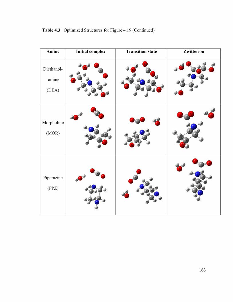
163



Diethanol-

-amine

(DEA)

Morpholine

(MOR)

Piperazine

(PPZ)

164

Table 4.4 Optimized Structures for Amines in Figure 4.21

Amine Initial complex Transition state Bicarbonate

Methyl

amine

(MA)

Propyl

amine

(PA)

Mono-

ethanol

amine

(MEA)

165



2-Amino -1-

propanol (AP)

2-Amino-

2-methyl-

1-propanol (AMP)

Dimethyl Amine (DMA)

166



Diethanol-

-amine

(DEA)

Morpholine

(MOR)

Piperazine

(PPZ)

167

4.4 CONCLUSIONS

Static calculations with PCM continuum model to determine dominant reaction

intermediates underscored the need for inclusion of explicit water molecules for realistic

modeling of the reaction pathways. Our DFT calculations with explicit water molecules

reveal, for the reaction involving one MEA molecule, that the CO2+MEA+nH2O reaction

proceeds as initial complex (IC)zwitterioncarbamatecarbamic acid. This 3-step

pathway was only seen when n, the number of explicit water molecules, is increased.

Instances of ICzwitterioncarbamic acid or ICcarbamic acid result with fewer

water molecules, and such results have been presented in the literature for years. Our

modeling is the first to correctly predict carbamate ions as the dominant product species.

The carbamate anion becomes thermodynamically competitive at neutral-pH and

dominant at basic-pH conditions, compared to both zwitterion and carbamic acid

intermediates, when properly solvated in the modeling.

Models involving two MEA molecules were deemed most relevant to modern-

day concentrated alkanolamine solutions. Such models, tried by others (Xie, Han,

Arstad), were improved incorporating further explicit water molecules. A tetramolecular

route (Shim 2008) featuring amine to amine proton transfer via water relay, was also

studied. Gradual incorporation of more water molecules shifted the zwitterion-

deprotonation transition state from “late” to “early,” and in a 2-amine-18-water model,

the predicted barrier is effectively non-existent (0.2 kcal/mol), suggesting that one could

consider the zwitterion as a species so short-lived that the Termolecular mechanism

168

would be dominant in concentrated alkanolamiane solutions. However, in dilute

solutions, when an amine is fully solvated by water molecules, single-MEA modeling

showed that zwitterion deprotonation will occur via a relay mechanism having a small

activation energy, making the Zwitterion mechanism more relevant. The relative

dominance of these mechanisms depends on amine concentration and thus explains

broken order kinetics. The results appear to dispel the Carbamic Acid mechanism,

revealing no thermodynamic drive for forming this intermediate.

To explore the idea of da Silva and Svendsen that the activation barrier of

carbamate formation comes from water displacement by CO2, the tricky zwitterion-

formation steps were searched for. As H2O molecules were explicitly added, activation

barriers rose, first due to breaking an initial amine…H2O hydrogen bond that impeded

the approach of CO2, and later due to differentials in total H-bonds in the model as CO2

formed the zwitterion. Thus their idea does seem plausible.

From the study with MEA we believe that the mechanism in aqueous

alkanolamine solution is heavily dependent on reaction environment of amine. For other

amines the effect of pKa on formation of zwitterion and bicarbonate was studied with

simple 6-atom cycles in neutral-pH modeling. It was discovered that secondary amines

have inherently greater CO2 affinity than primary amines when comparing amines of

same H+ affinity (pKa). Activation energies vary with pKa in a sufficient manner that this

effect could very well impinge on the importance (or non-importance) of a possible

zwitterion intermediate, and thus affect mechanism.

169

4.5 REFERENCES

1. Caplow, M. Kinetics of Carbamate Formation and Breakdown. J. Am. Chem.

Soc. 1968, 90,6795.

2. Dancwerts, P. V. The Reaction of CO2 with Ethanolamines. Chem. Eng. Sci.

1979, 34, 443.

3. Crooks, J. E.; Donnellan, J. P. Kinetics and Mechanism of the Reaction Between

Carbon Dioxide and Amines in Aqueous Solution. J. Chem. Soc, Perkin

Transactions 1989, 2, 331.

4. McCann, N.; Phan, D.; Wang, X.; Conway, W.; Burns, R.; Attalla, M.; Puxty, G.;

Maeder, M. Kinetics and Mechanism of Carbamate Formation from CO2 (Aq),

Carbonate Species, and Monoethanolamine in Aqueous Solution. J. Phys. Chem.

A 2009, 113, 5022.

5. Conway, W.; Wang, X.; Fernandes, D.; Burns, R.; lawrance, G.; Puxty, G.;

Maeder,M.Comprehensive Kinetic and Thermodynamic Study of the Reactions

of CO2(aq) and HCO3with Monoethanolamine (MEA) in Aqueous Solution. J.

Phys. Chem. A 2011, 115, 14340.

6. Versteeg, G. F.; van Swaaij, W. P. M. On the Kinetics Between CO2 and

Alkanolamines Both in Aqueous and Non-Aqueous Solutions-I. Primary And

Secondary Amines. Chem. Eng. Sci. 1987a, 43, 573..

7. Versteeg, G. F.; Van Dijck, L. A. J.; Van Swaaij, W. P. M. On the Kinetics

Between CO2 and Alkanolamines Both in Aqueous and Non-Aqueous Solutions.


170

8. Donaldson T. L.; Nguyen Y. N. Carbon Dioxide Reaction Kinetics and Transport

in Aqueous Amine Membranes. Ind. Eng. Chem. Fundam. 1980, 19, 260.

9. Tomasi J.; Mennucci B.; and Cammi R. Quantum Mechanical Continuum

Solvation Models. Chem. Rev., 2005, 105, 2999.

10. Cramer, C. J.; Truhlar D. G. A Universal Approach to Solvation Modeling. Acc.

Chem. Res. 2008, 41, 760.

11. Klamt A. and Schuurmann, G. COSMO: A New Approach to Dielectric

Screening in Solvents with Explicit Expressions for the Screening Energy and its

Gradient. J. Chem. Soc. Perkin Trans. 2 1993, 799.

12. Faurholt, C. Studies of Aqueous Solutions of Carbamates and Carbonates, J.

Chim. Phy. 1925, 22, 1-44.

13. Arstad, B.; Blom, R.; Swang O. CO2 Absorption in Aqueous Solutions of

Alkanolamines: Mechanistic Insight from Quantum Chemical Calculations. J.

Phys. Chem. A 2007, 111, 1222.

14. Shim, J. G.; Kim, J. H.; Jhon, Y. H.; Kim, J.; Cho, K. H. DFT Calculations on the

Role of Base in the Reaction Between CO2 and Monoethanolamine. Ind. Eng.

Chem. Res. 2009, 48, 2172.

15. Xie, H.-B.; Zhou, Y.; Zhang, Y.; Johnson, J. K. Reaction Mechanism of

Monoethanolamine with CO2 in Aqueous Solution from Molecular Modeling. J.

Phys. Chem. A 2010, 114, 11844.

16. Han, B.; Zhou, C.; Wu, J.; Tempel, J. T.; Cheng, H. Understanding CO2 Capture


Phys. Chem. Lett. 2011, 2,522.

171

17. Ismael, M.; Sahnoun, R.; Suzuki, A.; Koyama, M.; Tsuboi, H.; Hatakeyama,N.;

Endou, A.; Takaba, H.; Kubo, M.; Shimizu, S.;Carpio, C. A. D.; Miyamoto, A.

A DFT Sudy on the Carbamates Formation through the Absorption of CO2 by

AMP. Int. J. of Greenhouse Gas Control 2009, 3, 612.

18. Yamada, H.; Matsuzaki, Y.; Higashii, T.; Kazama, S. Density Functional Theory

Study on Carbon Dioxide Absorption into Aqueous Solutions of 2-Amino-2-

Methyl-1-Propanol Using A Continuum Solvation Model. J. Phys. Chem.

A 2011, 115, 3079.

19. da Silva, E. F., Svendsen, H. F. Ab Initio Study of the Reaction of Carbamate

Formation from CO2 and Alkanolamines. Ind. Eng. Chem. Res. 2004, 43, 3413.

20. Gaussian 09, Revision B.01, M. J. Frisch, G. W. Trucks, H. B. Schlegel, G. E.

Scuseria, M. A. Robb, J. R. Cheeseman, G. Scalmani, V. Barone, B. Mennucci,

G. A. Petersson, H. Nakatsuji, M. Caricato, X. Li, H. P. Hratchian, A. F.

Izmaylov, J. Bloino, G. Zheng, J. L. Sonnenberg, M. Hada, M. Ehara, K. Toyota,

R. Fukuda, J. Hasegawa, M. Ishida, T. Nakajima, Y. Honda, O. Kitao, H. Nakai,

T. Vreven, J. A. Montgomery, Jr., J. E. Peralta, F. Ogliaro, M. Bearpark, J. J.

Heyd, E. Brothers, K. N. Kudin, V. N. Staroverov, R. Kobayashi, J. Normand, K.

Raghavachari, A. Rendell, J. C. Burant, S. S. Iyengar, J. Tomasi, M. Cossi, N.

Rega, J. M. Millam, M. Klene, J. E. Knox, J. B. Cross, V. Bakken, C. Adamo, J.

Jaramillo, R. Gomperts, R. E. Stratmann, O. Yazyev, A. J. Austin, R. Cammi, C.

Pomelli, J. W. Ochterski, R. L. Martin, K. Morokuma, V. G. Zakrzewski, G. A.

Voth, P. Salvador, J. J. Dannenberg, S. Dapprich, A. D. Daniels, Ö. Farkas, J. B.

172

Foresman, J. V. Ortiz, J. Cioslowski, and D. J. Fox, Gaussian, Inc., Wallingford

CT, 2009.

21. Becke, A. D. Density-Functional Thermochemistry. III. The Role Of Exact

Exchange. J.Chem.Phys. 1993, 98, 5648.

22. Stephens, P. J. ; Devlin, F. J.; Chabalowski, C. F.; Frisch, M. Ab Initio

Calculation of Vibrational Absorption and Circular Dichroism Spectra Using

Density Functional Force Fields. J. Phys. Chem. 1994, 98, 11623.

23. Cossi, M., Barone, V., Cammi, R., Tomasi, J. Ab Initio Study of Solvated

Molecules: A New Implementation of The Polarizable Continuum Model. Chem.

Phys. Lett. 1996, 255, 327.

24. Baker J. An Algorithm for the Location of Transition-States. J. Comp. Chem.

1986, 7, 385.

25. Wang, T-.T; Bishop S. H.; Himoe, A. Detection of Carbamate as A Product of

the Carbamate Kinase-Catalyzed Reaction by Stopped Flow Spectrophotometry.

J. Biol. Chem. 1972, 247, 14, 4437.

26. Aboudheir, A.; Tontiwachwuthikul, P.; Chakma, A.; Idem, R. Kinetics of the

Reactive Absorption of Carbon Dioxide in High CO2-Loaded, Concentrated

Aqueous Monoethanolamine Solutions. Chem. Eng. Sci. 2003, 50, 1071.

173

Chapter 5: Molecular Dynamics Simulation of CO2/Amine/Water Mixtures

_______________________________________________________________________

5.1 INTRODUCTION

The prediction of small, 4 kcal/mol activation energies (Ea) for interconversion of

zwitterion-to-carbamate-to-carbamic acid in the previous chapter (Figure 4.6) come with

an important caution: they are for only one pathway, and others might be possible with

lower Ea values. In this chapter, results from ab initio molecular dynamics (AIMD)

simulations are shown, providing a complementary study of intermediate stabilities.

AIMD includes the effect of temperature and searches for reaction paths in an unbiased

way. These AIMD simulations were performed in tandem with the calculations of the

previous chapter.

Recently two AIMD simulation papers have been published that observed the

fate of MEA-zwitterion. Han et al. (2011)1 studied the reaction of MEA-zwitterion in

presence of another MEA and 16 water molecules (approx. 30 wt% solution) and found

that the MEA-zwitterion reacted with MEA in 4 ps, the reaction barrier was 1.3 kcal/mol

and heat of absorption was -22 kcal/mol. Guido et al. (2013)2 studied the fate of a MEA-

zwitterion in 122 water molecules (approximately 3 wt% aqueous solution) and observed

that both forward reaction (deprotonation by water) and backward reaction (CO2 release)

are characterized by free-energy barriers of 6−8 kcal/mol and thus competitive. Both

174

researchers have underscored the importance of explicit water molecules in the model: to

reach quantitative agreement with the experimental heat of absorption value (Han, et

al,.2011)1 and to see the large entropic effect in the conversion of zwitterion (Guido et

al., 2013)2 both in forward and backward direction.

The first objective of the simulations was to see the fate of all possible

intermediates, in the bicarbonate (Group I) and carbamate (Group II) pathways (Figures

5.1 and 5.2), on an extremely limited 8 ps timescale, to see if all intermediates are indeed

separated by some sort of potential barrier. The second objective was to try some longer

simulations with a variety of amines to see if a complete transformation from carbamate

zwitterion to carbamic acid could be found (Group III). The third objective was to

explore the reactivity of the carbamate zwitterion in the presence of a nearby amine

molecule (Group IV).

Figure 5.1 Possible intermediates in the bicarbonate pathway in CO2/H2O system

Figure 5.2 Possible intermediates in the carbamate pathway in CO2/Me2NH/H2O system

+ H2O

HO

HC

O

O HOC

O

O HOC

O

OH

OC

O

+H

OH

+ H2O + H3O+ + H2O

carbonatezwitterion

bicarbonate carbonic acid

+ H2O

MeNH

Me

CO

O MeNC

O

O MeNC

O

OH

OC

O

+Me

HNMe

+ H2O + H3O+ + H2O

carbamatezwitterion

carbamate carbamic acid

Me Me

175

5.2 METHOD

The simulations were performed using the Vienna Ab Initio Simulation Package

(VASP)3,4 version 5.2.11 on the in-house supercomputer Dextrose. The following VASP

specifications were used in all simulations: the potpaw GGA plane-wave basis sets,5,6

standard precision (PREC=Normal); ENMAX=400eV; a Nosé thermostat for canonical

(NVT) conditions7 with 40 fs thermal oscillations (SMASS=0), a Verlet velocity

algorithm;8 a temperature of 313K (40°C), and a time step equaling 1 fs of real time.

The sample cell was cubic in shape and replicated using periodic boundary conditions to

mimic the bulk liquid. The forces used in the simulations were of the PW91 level of

density functional theory (DFT)9,10 but with a Grimme-style semi-empirical van der

Waals (vdW) attractive potential added on to the energy and force calculations.

First, 64 water molecules in a cubic box of width 12.45 Å were simulated for

8000 fs at 40°C, generating a pseudo-equilibrated water sample, Geometry A (step

8001). Another simulation was run for 24000 fs starting from geometry A, generating a

further equilibrated sample, Geometry B (step 32001). Then, starting with geometries A

and B respectively, starting ensembles for each group I and Group II “production run” at

40°C were made by substituting a solute molecule for a small number of water

molecules:

176

Group –I. 8-ps simulations of water-CO2 system (Figure 5.1)

a) Replace a H2O with a CO2

b) Replace two H2O with the carbonate zwitterion

c) Replace two H2O with bicarbonate, and one H2O with an H3O+

d) Replace two H2O with carbonic acid

Group –II. 8-ps simulations of water-CO2-dimethylamine system (Figure 5.2)

e) Replace four H2O with the carbamate zwitterion

f) Replace four H2O with carbamate, and one H2O with an H3O+

g) Replace four H2O with carbamic acid

A 8-ps continuation run (e2) of dimethyalamine-zwitterion was performed

starting with the final geometry obtained from simulation (e). The final geometry of run

e2 (geometry C) was the starting point of all the secondary amine zwitterion simulations

(h, l, m, and n) in Groups III and IV (prepared by suitable modification of geometry C).

Starting ensembles for Groups III and IV simulations (i, j, k, o) with primary amines

(methylamine, monoethanolamine and 2-methyl-2-amino-propanol (AMP)) were

prepared by solute replacement in geometry B.

Group –III. Longer zwitterion simulations

h) Dimethylamine (Me2NH) zwitterion, starting from geometry C

i) Replace four water molecules with methylamine (MeNH2) zwitterion

j) Replace five water molecules with monoethanolamine (MEA) zwitterion

177

k) Replace five water molecules with AMP-zwitterion and increase the cell

width to 12.59 Å (to match the density with that of experimental value)

l) Replace Me2NH-zwitterion with diethanolamine (DEA)-zwitterion

m) Replace Me2NH -zwitterion and one water molecule with PPZ-zwitterion

Group –IV. Zwitterion+amine simulation

n) Replace three water molecules with Me2NH

o) Replace seven water molecules with MeNH2-zwitterion and MeNH2

178

5.3 RESULTS

5.3.1 Group –I. 8-ps simulations of water-CO2 system

Results of 8-ps long simulations of pure CO2, carbonate zwitterion, bicarbonate

ion and bicarbonic acid (Figure 5.1) are presented.

a) Simulation of aqueous CO2

No reaction was observed in the 8 ps-long run.

b) Simulation of aqueous carbonate zwitterion

The carbonate zwitterion (Figure 5.3) immediately broke into water and CO2 by

O-C bond cleavage. The O-C bond length increases up to 4.25 Å in very short time

(within 20fs) and the CO2 and water does not return as close as 2.5 Å.

Figure 5.3 Starting geometry in simulation (b), showing only two of the neighboring

water molecules.

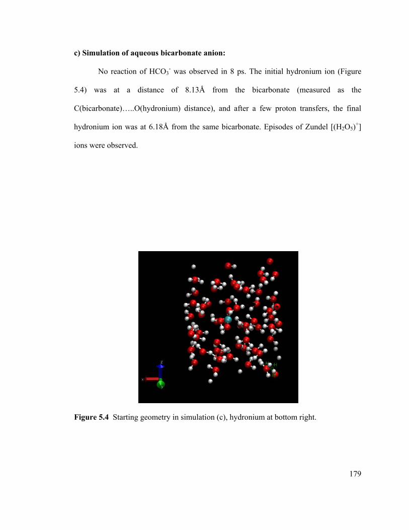
179

c) Simulation of aqueous bicarbonate anion:

No reaction of HCO3- was observed in 8 ps. The initial hydronium ion (Figure

5.4) was at a distance of 8.13Å from the bicarbonate (measured as the

C(bicarbonate)…..O(hydronium) distance), and after a few proton transfers, the final

hydronium ion was at 6.18Å from the same bicarbonate. Episodes of Zundel [(H2O5)+]

ions were observed.

Figure 5.4 Starting geometry in simulation (c), hydronium at bottom right.

180

d) Simulation of aqueous carbonic acid

H2CO3 dissociated into HCO3- + H+ after 4.7 ps (Figure 5.5). Initially placed

without hydrogen bonds, the H2CO3 formed simultaneous OH-O bonds with two

neighboring water molecules after 600 fs (Figure 5.5, inset).

Figure 5.5 Evolution of two OH bond lengths in simulation (d), demonstrating

ionization of H2CO3 at 4.7 ps.

181

5.3.2 Group –II. 8-ps simulations of water-CO2-dimethyl amine system

Results of simulations of intermediates that appear through pathway II (Figure

5.2) in CO2-aqueous dimethylamine (Me2NH) system are described.

e) Simulation of aqueous carbamate zwitterion

The zwitterion (initial geometry shown in Figure 5.6) persisted for 8ps.

Figure 5.6 Starting geometry in simulation (e), showing only three of the neighboring

water molecules. The N-C bond length is 1.6 Å and the NH..OH2 bond

length (broken line) is 2.31 Å

182

f) Simulation of aqueous carbamate anion

Carbamate interconverted with carbamic acid many times (Figures 5.7 and 5.8).

t=0fs, carbamate + H3O+

t=5191fs , carbamic acid

Figure 5.7 Initial local geometry of carbamate and hydronium ion (left) and local

geometry of carbamic acid formed at t=5191fs (right) in simulation (f).

Figure 5.8 Evolution of the OH distance that demonstrates the interconversion of

carbamate with carbamic acid in simulation (f). The proton, initially in the

hydronium ion, approaches from an initial distance of 3.01Å to the

carbamate anion.

183

g) Simulation of aqueous carbamic acid

The carbamic acid (CH3)2NCOOH dissociated into (CH3)2NCOO– and H+ at

t=6.5 ps. Figure 5.9 show the initial acid and final anion surrounded by water molecules

respectively. The conversion of carbamic acid into carbamate is captured in Figure 5.10:

The OH bond in the carbamic acid (blue line) becomes hydrogen bonded at 3ps which

causes the OH bond to vibrate more vigorously. Dissociation occurs at 6.5 ps to form

carbamate. The red line depicts the distance between the proton of carbamic acid and the

oxygen of a neighboring water molecule which finally abstracted the proton.

t=0,Carbamic acid

t=8001fs, Carbamate

Figure 5.9 Initial geometry of carbamic acid (left); and geometry of carbamate anion at

t=8001fs (right) in simulation (g). Only few water molecules are shown.

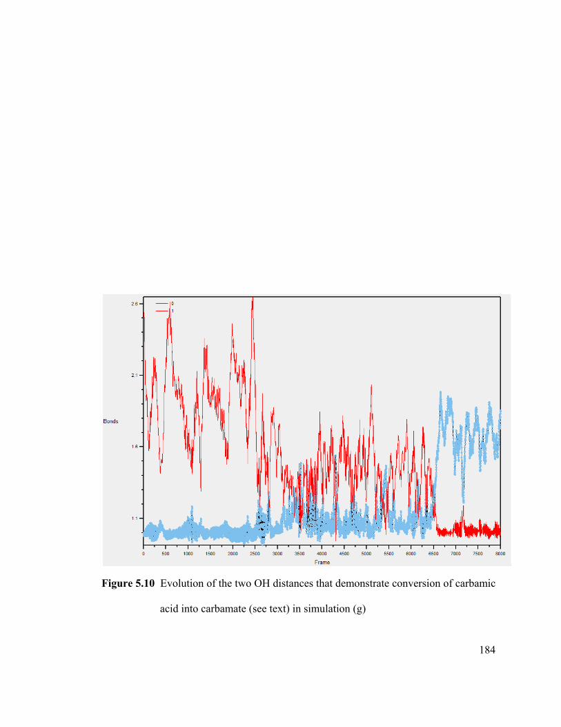
184

Figure 5.10 Evolution of the two OH distances that demonstrate conversion of carbamic

acid into carbamate (see text) in simulation (g)

185

5.3.3 Group-III. longer zwitterion simulations

Results for longer simulations, hoping to see a zwitterion ↔ carbamate transition,

are presented.

h) Dimethylamine zwitterion.

An 8 ps continuation run (Run e2) of simulation (e) also revealed no change, so a

further 100 ps continuation run (simulation (h)) was performed. In this 3rd run, the

zwitterion converted into carbamate at 8 ps (Figure 5.11), and then, the carbamate

converted into carbamic acid at 13 ps (Figure 5.12). The breaking of NH bond to form

carbamate also simultaneously caused the equilibrium NC bond-length to shrink (the

second plateau in the red line in Figure 5.11).

The reaction from zwitterion to carbamic acid via carbamate proceeded via

proton relay through a hydrogen-bonded 10-atom cycle formed by participation of three

solvent water molecules and the zwitterion (Figure 5.13). The lengths of four new OH

bonds that are formed during the relay are tabulated as a function of time in run (h) in

Table 2. Prior to zwitterion-deprotonation, at 8 ps, solvent molecules reoriented to

bridge the two polar ends of a OCNH segment of zwitterion; forming the “hydrogen-

bonded” cycle through which the two elementary reactions ‘zwitterion carbamate’

and ‘carbamate carbamic acid’ took place via proton transfer relay.

The carbamic acid formed at 13 ps lasted for only about 1 ps; then, it lost its

gained H+ at 14 ps (re-forming carbamate) and did not convert back into carbamic acid

until 95 ps where it stayed for the remaining 5 ps of run (h) (Figure 5.12).

186

Figure 5.11 The breaking of NH (blue) and simultaneous shrinking of NC(red) bond

lengths in simulation (h).

187

Figure 5.12 Evolution of two OH bond lengths in simulation (h), the oxygens being the

two in COO moiety.

188

Figure 5.13 The 10-atom cycle at t=8ps in simulation (h) (all surrounding water

molecules are removed). Some bond lengths are provided in Table 5.1.

Table 5.1 Bond-Formation through 10-Atom Cycle Schematically Shown in Figure

5.13

At t=6ps, all of these OH distances are too long to be considered covalent bond;

but at 13ps, all of them are considered to be covalent bonds. formation of bond O3H8 is

complete by 9 ps, bond O1 H 21 by 11 ps, bonds O2 H11 and O4H17 by 13 ps.

Time(ps) O3H18 O1H21 O2H11 O4H176 1.66 1.97 3.71 1.797 1.61 2.4 1.76 1.878 1.37 1.6 1.54 1.89 0.96 1.73 1.57 1.59

11 0.98 0.97 1.74 1.7212.5 0.98 1.05 1.13 1.5113 1 1.06 1 1.04

Distance (Å)

189

i) Methylamine (MeNH2) zwitterion

Only one 8-ps simulation ( run i) was needed to observe the MeNH2-zwitterion

(Figure 5.14) convert into carbamate at 0.9 ps and then into carbamic acid at 1.5 ps

(Figure 5.15). During the time period 1.5ps <t<3.8ps , carbamate interconverted with

carbamic acid and afterwards the carbamic acid persisted.

Figure 5.14 Starting geometry in simulation (i), showing only five of the neighboring

water molecules. The NH-OH2 bond length is 1.75 Å (H21O6) and the

O7H19 distance is 1.81 Å. The other NH bond was not hydrogen-bonded

to any water molecules in the starting geometry

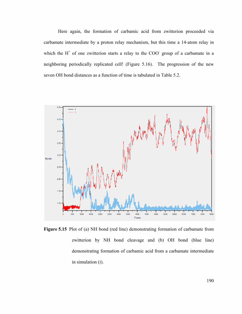
190

Here again, the formation of carbamic acid from zwitterion proceeded via

carbamate intermediate by a proton relay mechanism, but this time a 14-atom relay in

which the H+ of one zwitterion starts a relay to the COO- group of a carbamate in a

neighboring periodically replicated cell! (Figure 5.16). The progression of the new

seven OH bond distances as a function of time is tabulated in Table 5.2.

Figure 5.15 Plot of (a) NH bond (red line) demonstrating formation of carbamate from

zwitterion by NH bond cleavage and (b) OH bond (blue line)

demonstrating formation of carbamic acid from a carbamate intermediate

in simulation (i).

191

Table 5.2 Evolution of Some Bond Lengths as a Function of Time Through the 14-atom

Relay Shown in Figure 5.16

Figure 5.16 t=1437fs of simulation (i), showing the 14-atom relay trajectory (connected

by broken lines), the surrounding water molecules are removed

Time(ps) O28H43 O29H40 O5H41 O1H22 O2H12 O7H14 N8C90.3 1.69 1.72 1.9 2.12 1.58 2.47 1.830.5 1.45 1.87 1.68 1.75 1.81 1.86 1.560.9 1.35 1.48 1.87 2.23 1.7 1.8 1.51.1 0.99 1.2 1.52 1.96 1.67 1.69 1.37

1.437 1.03 0.96 1.02 1.05 1.2 1.62 1.441.6 0.96 0.98 0.97 1.01 1.03 1.03 1.347 0.94 1.02 0.99 0.99 1.02 1.04 1.38

Distance (Å)

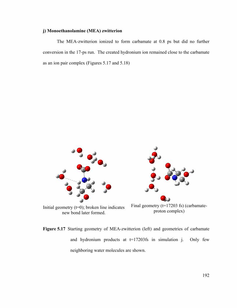
192

j) Monoethanolamine (MEA) zwitterion

The MEA-zwitterion ionized to form carbamate at 0.8 ps but did no further

conversion in the 17-ps run. The created hydronium ion remained close to the carbamate

as an ion pair complex (Figures 5.17 and 5.18)

Initial geometry (t=0); broken line indicates

new bond later formed.

Final geometry (t=17203 fs) (carbamate-

proton complex)

Figure 5.17 Starting geometry of MEA-zwitterion (left) and geometries of carbamate

and hydronium products at t=17203fs in simulation j. Only few

neighboring water molecules are shown.

193

Figure 5.18 Evolution of three OH bond lengths in the generated hydronium ion in

simulation (j).

194

k) 2-amino-2-methyl propanolamine (AMP) zwitterion

An AMP-zwitterion (Figure 5.19) was simulated in 59 water molecules for 110

ps (initial run of 8ps, followed by two continuation runs of 8 ps and 94-ps) and no

change occurred. Two 12-atom H-bonded cycles formed at 80 ps in the final 94-ps run.

Figure 5.19 Starting geometry of AMP-zwitterion in simulation (k), only few

neighboring water molecules are shown.

l) Simulations with diethanolamine (DEA) zwitterion

A DEA-zwitterion (Figure 5.20) was simulated in 60 water molecules for 16203

fs, and no reaction was observed. A tight 6-atom cycle formed at 15 ps and lasted for the

remaining 1 ps.

Figure 5.20 Starting geometry of zwitterion in simulation (l): H22O2=3.1 Ǻ,

H21O5=1.79 Ǻ, H22O4=1.86 Ǻ.

195

m) Piperazine (PPZ) zwitterion

PPZ-zwitterion was simulated in 59 water molecules for 15 ps and no reaction

was observed. Cyclic arrangement of water molecules around the OCNH segment could

be identified after 11 ps. A 10-atom cycle around the OCNH segment (Figure 5.21, right)

and a 14-atom cycle connecting the same OC moiety to the other NH had formed by 15-

ps.

As a side note, the simulation data reveals the weakening of the NH bond upon

carboxylation, by a comparison of N- vibration amplitudes (Figure 5.22).

Initial geometry

t=15ps NH=1.1 Ǻ, NH-O=1.66 Ǻ

Figure 5.21 Starting geometry (left) of PPZ-zwitterion in simulation (m), few

surrounding water molecules are shown. 10-atom cycle at 15-ps (right).

196

Figure 5.22 Difference in amplitude of vibration of two NH bond lengths of PPZ-

zwitterion in simulation (m), (red: 3-coordinated N, blue: 4-coordinated

N).

197

5.3.4 Group-IV. simulations of zwitterion+amine

We did two simulations at higher amine concentration to see potential proton

transfer from zwitterion to amine.

n) Simulation of Me2NH+COO- + Me2NH

A dimethylamine-zwitterion was simulated in presence of another nearby neutral

dimethaylamine in 57 water molecules for 48 ps (24 ps and its continuation for another

24 ps). The initial geometry is shown in Figure 5.23, with the NH bond of zwitterion

pointing towards a water molecule (NH-O=2.31 Ǻ). The neutral amine was placed at a

N to N distance of 4.66 Ǻ from the zwitterion, and its lone pair was pointing towards

another water molecule (the N-HO distance is 1.66 Ǻ).

t=0, (dimethylamine-zwitterion+neutral

dimethylamine), N-N=4.66 Ǻ

t=48 ps (carbamate+protonated

dimethylamine), NH-O=1.74A, N-N=3.71Ǻ

Figure 5.23 Initial geometry (left) and final geometry (right) in simulation (n), only few

water molecules are shown.

198

Zwitterion deprotonated at 27.9 ps (Figure 5.24) . By 28.2 ps, a 14-atom H-

shuttling cycle stopped just short of forming a carbamic acid, staying as a carbamate-

hydronium complex (Figure 5.25). From 28.3 to 29.5 ps, an H-shuttling relay occurred

back-and-forth before finally resting with the extra H+ on the uncarboxylated amine

molecule. This final state persisted until the end of the 48 ps simulation. 11 water

molecules were involved in the relay of proton from the zwitterion to the neutral amine

and the time required was less than 2 ps.

199

Figure 5.24 Evolution of some important bond lengths in simulation (n). Red: breaking

of zwitterion NH bond; light blue: formation of NH bond in protonated

dimethylamine; green: shrinking of NC bond length immediately after

deprotonation (N becomes positively charged); dark blue: evolution of an

OH bond length in carbamate-hydronium complex.

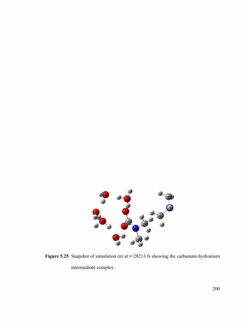
200

Figure 5.25 Snapshot of simulation (n) at t=28213 fs showing the carbamate-hydronium

intermediate complex.

201

o) Simulation of MeNH2-zwitterion + MeNH2.

A MeNH2-zwitterion-like structure (Figure 5.26, top left) was simulated for 8-ps

in 57 water molecules plus a nearby MeNH2 molecule in cell of width 12.45 Ǻ.

Zwitterion was formed in 150 fs (NC bond length decreased to 1.54 Ǻ from initial 2 Ǻ)

which converted to carbamate by H-shuttling to neutral MeNH2 via a water molecule at

t~380 fs. The ions later approached each other and formed a cation-anion complex

(Figure 5.26, bottom right).

Starting geometry N5C7=2 Ǻ;H12O1=2.58 Ǻ H10N4=3.42 Ǻ

t=320fs,NC7=1.6Ǻ,H12O1=1.56Ǻ H10N4=1.67 Ǻ

t=380fs NC7=1.52 Ǻ;H12O1=1.06 Ǻ ; H10N4=1.10 Ǻ

t=8001fs,NC7=1.39 Ǻ;H12O1=1.02 Ǻ; H10N4=1.07 Ǻ;O2H17=1.58 Ǻ

Figure 5.26 Geometries in simulation (o) without the spectator water molecules.

Conversion of zwitterion to carbamate happens through proton relay to a

nearby amine.

202

5.4 CONCLUSIONS

Group I simulations of aqueous CO2, H2OCO2 zwitterion, HCO3- (with faraway

H3O+), and H2CO3 did the following: CO2 did not react, H2OCO2 fell back to CO2,

HCO3- did not react, and H2CO3 persisted for 5 ps before changing to HCO3

- for its final

3ps. What does this tell us? Firstly, the bicarbonate zwitterion seems to have no

stability at all, suggesting that a “wider” barrier exists between an encounter complex

and the bicarbonate/carbonic acid equilibrium, and secondly that the HCO3-/H2CO3

equilibration is too slow for us to conclude which one is dominant.

Group II simulations of Me2NHCO2 zwitterion, Me2NCO2- (with far away H3O

+),

and Me2NCOOH did the following: the zwitterion did not react, Me2NCO2- went back-

and-forth with the acid roughly once per ps, and the acid persisted 6.5 ps before

converting to the anion for 1.5 ps. What does this tell us? Firstly, that Me2NHCO2

zwitterion is more stable than the H2OCO2 zwitterion and thus deserves consideration as

an intermediate, and is separated from the anion/acid equilibrium pair by some sort of

barrier; and secondly that the Me2NCO2-/Me2NCOOH equilibration is too slow for us to

conclude which one is dominant. The anion and acid interconverted on a very short

timescale, suggesting that anion/acid equilibria are fairly barrierless, and hence

thermodynamics will determine the ratio of anion to acid.

Group III simulations of various carbamate-zwitterions revealed forward

conversion of zwitterions in 3 of the 6 cases: Me2NH-zwitterion, MeNH2-zwitterion and

MEA-zwitterion. Of these, only MEA-zwitterion failed to show carbamate/carbamic acid

equilibrium. Reaction of AMP-zwitterion, DEA-zwitterion and PPZ-zwitterion was not

203

observed in 110 ps, 16 ps, and 15 ps long runs, respectively. However, a common role

of solvent was identified in all six simulations: solvent molecules reoriented to bridge the

two polar ends of a OCNH segment of zwitterions, forming a “hydrogen-bonded” cycle

(if N water molecules participate, the cycle has 4+2N atoms, and 2+N covalent bonds

before any reaction takes place). These cycles likely occur in reality.

We highlight that the H-shuttling cycles seen in Group III simulations do not

exist in aqueous amine solution prior to absorption of CO2. The preexisting H-bond

networks must be reformed to connect to the negative OC segment of COO moiety. This

reorientation process can be considered as the minimum lifetime of zwitterions when a

nearby amine is absent. Both of the NH bonds of primary amines (and piperazine) were

seen active in formation of such cycles. The number of water molecules involved in

such cycles changes over course of time. Although the reaction was not observed in

simulations k-m, this could be due to the time limitation of our simulations.

The Group IV simulations of zwitterion in presence of nearby amine showed

H2O-mediated H+ transfer relays to form carbamate and protonated amine, products

which corroborate with experimental observation. The lengths of the relay were 11 H2O

(simulation ‘n’) and 1 H2O (simulation ‘o’). The previously described H-bonded cycle

for forming carbamic acid formed in simulation ‘n’. The speed of the reaction in

simulation ‘o’ (less than 0.5 ps) reveals that zwitterion lifetime and the formation of

carbamic acid is hindered by high amine concentrations, which put two amine molecules

in closer proximity. It also suggests that the zwitterion lifetime might be reduced even

further if the two amine molecules were directly bonded to each other.

204

An amine-to-amine proton transfer was observed in 0.5 ps in a simulation1 where

the neutral amine molecule was placed close to the zwitterion (the NH bond of zwitterion

pointed to the lone pair of neutral amine). But, classical MD simulations of aqueous

monoethanol amine showed significantly less frequent N-HN hydrogen bonding

interactions in aqueous solution than in pure liquid amine.11-15 Further work needs be

done in that area which will shed further light on zwitterion stability (lifetime) and the

fate of H-bonded cycles in case of direct proton transfer.

The observation of 10- to14-atom H+-shuttling cycles for formation of carbamic

acid (via carbamate from zwitterion) justifies our study of such multiple-water-mediated

pathways in our static calculations in Chapter 4. Indeed, such pentamolecular and

hexamolecular pathways have never been postulated, and it is hoped that these new paths

and the results of Chapter 4 will significantly advance the efforts to finally solve this

mechanism.

205

5.4 REFERENCES

1. Han, B.; Zhou, C.; Wu, J.; Tempel, J. T.; Cheng, H. Understanding CO2 Capture


Phys. Chem. Lett. 2011, 2, 522.

2. Guido C. A., Pietrucci F., Gallet G. A.; Andreoni W. The Fate of a Zwitterion in

Water from ab Initio Molecular Dynamics:Monoethanolamine (MEA)-CO2. J.

Chem. Theory Comput. 2013, 9, 28.

3. Kresse G.; Hafner J. Ab Initio Molecular Dynamics for Liquid Metals. Phys. Rev.

B 1993, 47, 558.

4. Kresse G.; Furthmüller J. Efficient Iterative Schemes for Ab Initio Total-Energy

Calculations Using A Plane-Wave Basis Set. Phys. Rev B 1996, 54, 11169.

5. Kresse G.; Hafner, J. Norm-Conserving and Ultrasoft Pseudopotentials for First-

Row and Transition Elements. J. Phys. Condens. Matter 1994, 6, 8245

6. Kresse, G.; Joubert D. From Ultrasoft Pseudopotentials to the Projector

Augmented-Wave Method. Phys. Rev. B 1999, 59, 1758

7. Nos’e, S., A Unified Formulation Of The constant Temperature Molecular

Dynamics Methods. J. Chem. Phys. 1984, 81, 511.

8. Leach, A. R. Molecular Modeling: Principles & Applications, 2nd ed. Pearson,

Harlow, UK, 2001.

9. Perdew, J. P.; Chevary; J. A.; Vosko; S. H.; Jacson; K. A. ; Pederson; M. R. ;

Sing D. J.; Fiolhais; C. Atoms, Molecules, Solids, and Surfaces: Applications of

206

the Generalized Gradient Approximation for Exchange and Correlation. Phys.

Rev. B 1992, 46, 6671.

10. Grimme, S. Semiempirical GGA-Type Density Functional Constructed with a

Long-Range Dispersion Correction. J. Comput. Chem. 2006, 27, 1787.

11. Button, J. K.; Gubbins, K. E.; Tanaka, H.; Nakanishi, K. Molecular Dynamics

Simulation of the Hydrogen Bonding in Monoethanolamine. Fluid Phase

Equilib. 1996, 116, 320.

12. Alejandre, J.; Rivera, J. L.; Mora, M. A.; de la Garza, V. Force Field of

Monoethanolamine. J. Phys. Chem. B 2000, 104,1332.


Ethylene Glycol, Ethylenediamine, and 2-Aminoethanol. 1. The Local Structure

in Pure Liquids. J. Phys. Chem. A 2004, 108, 7151.

14. da Silva, E. F.; Kuznetsova, T.; Kvamme, B.; Merz, K. M., Jr. Molecular

Dynamics Study of Ethanolamine as a Pure Liquid and in Aqueous Solution. J.

Phys. Chem. B 2007, 111, 695.


Ethylene Glycol, Ethylenediamine, and 2-Aminoethanol. 2. Structure in Aqueous

Solutions. J. Phys. Chem. A 2004, 108, 7165.

207

Chapter 6: Screening of Ionic Liquids: A COSMO-RS Study†

_______________________________________________________________________

6.1 INTRODUCTION

The changing chemical composition of earth’s atmosphere, due to the colossal

rate of anthropogenic emission of CO2 produced from the burning of carbonaceous

fuel, warrants the necessity of the immediate abatement of CO2 emission.1 Such

concern, coupled with the prospect of the utilization of captured CO2 in enhanced oil

recovery,2 has propelled research efforts to develop affordable and environmentally

benign technologies for CO2 capture from large emission sources. The most

industrially advanced technology for CO2 capture, at present, is chemical absorption

of CO2 with aqueous alkanolamine solutions, which are, in general, volatile, prone to

degradation and equipment corrosion, and most importantly, energy-intensive to

regenerate.3 While energy and cost-efficient novel amine solvents are continually

investigated,4-6 the exploration of other advanced materials for CO2 are being

sought.7 Among the many innovative technologies, ionic liquids are identified as

potential solvents for developing green CO2 capture technology with significant cost

reduction benefit.8

_______________________________________________________________________ †This chapter contains material reproduced with permission from Sumon, K. Z.; Henni, A. Ionic liquids for CO2 capture using COSMO-RS: Effect of structure, properties and molecular interactions on solubility and selectivity. Fluid Phase Equilib. 2011, 310, 39-55. Copyright © 2011 Elsevier B.V.

208

Ionic liquids (ILs) are the generic names of a broad category of salts with

melting point less than 100 °C. They are usually composed of large, asymmetric and

loosely coordinating organic cations and inorganic or organic anions. Due to their

ionic nature and high thermal stability, they tend to have negligible vapour pressure

making them, in general, environmentally benign as well as suitable for gas

separation without solvent loss or contamination of the vapour phase. The potential

of ionic liquids for CO2 capture was recognized first by researchers at the University

of Notre Dame.9 Since then, research efforts in this area have been expanding.10-14

Opportunities exist to generate task-specific ionic liquids by chemical alteration of

the cation or anion such as tethering a specific functional group in one of the

comprising ions.15-20 Different combinations between a variety of cations and anions

result in a large array of ionic liquids with unique properties. Experimental

investigation of ionic liquids is a challenging task due to their increasing number, and

for now, high cost. Therefore, screening and designing of ionic liquids for CO2

capture with a reliable computational method would be of great value for subsequent

experimental work. The present work is a contribution to such an objective.

Many attempts were made to model and predict the solubility of CO2 in some

limited number of ionic liquids based on group contribution method,21 regular solution

theory,22-24 Quantitative Structure Property Relationship (QSPR) method,25 Equation of

State,26 Conductor-like Screening Model for Real Solvents (COSMO-RS) method,27

molecular dynamics (MD)28-34 and Monte Carlo35 simulations. Among them, COSMO-

RS is suitable for fast screening of a large number of novel solvents as it does not require

any compound or group specific interaction parameters. COSMO-RS was shown useful

209

for qualitative prediction of solubilities of gases by a number of studies.36-40 Henry’s law

constants for CO2 in many ionic liquids were compared with experimental values.27,36-39

Ionic liquids were screened for CO2 capture from a pool of 408 ionic liquids by Zhang et

al.,36 170 ILs by Palomar et al.38 and 224 ILs by Gozalez-Miquel et al.39 based on

COSMO-RS prediction of Henry’s law constants of CO236,38 and N2

39 at 25°C. A

combination of COMSO-RS approach with equation of state was successfully used for

prediction and screening of CO2solubility at from (20 to 60) °C and upto the critical

pressure of CO2.40 Anions with fluorine,36,38,41 bromine38 and cations based on

guanidinium and phosphonium41 were shown to have high CO2 absorption capabilities.

At the molecular level, high CO2 absorption was related to the strong vdW interaction

with IL38 and consequently with higher exothermicity. ILs with thiocyanate anions were

found39 to enhance CO2/N2 selectivity due to enhanced vdW interactions preferentially

with CO2 while showing almost no affinity for N2. Shimoyama et al.42 used the model

COMSO-SAC43 for prediction of solubilities, selectivities and permeabilities for CO2 in

ionic liquids with imidazolium cations.

In the present work, we further explore the capabilities and limitation of

COMSOtherm44 that implements COSMO-RS as an a priori auxiliary tool in

screening and designing of ILs for CO2 capture. Henry’s law constants (HLC) of

CO2, CH4 and N2 and selectivities45 for the CO2/CH4 and CO2/N2 separation as a

function of temperature in an extended database of 2701 ILs is predicted. Structural

modifications that promote or diminish the solubility and selectivity are categorized.

Molecular interactions is elucidated through COSMO-RS derived a priori solvent

properties of IL such as sigma profiles and sigma-potentials, and a posteriori

210

quantities such as activity coefficients and transfer properties like enthalpy and

entropies of solvation. A new polarity parameter is introduced and the effect of

molar volume and polarity of ILs on solubility and selectivity is discussed.

COSMOtherm predictions of Henry’s law constants, selectivities, enthalpies of

solvation are compared with experimental results. Henry’s law constants predicted

by different researchers are also compared.

6.2 THEORY

COSMO-RS is an excess Gibbs energy model for liquid mixtures based on

surface charge interaction. Details of COSMO and COSMO-RS model is given in

references.46-50 The surface of a molecule or ion is divided into segments of a

standard area. Each segment is identified by its average screening charge obtained

from COSMO calculation. A histogram that shows the number of segments versus

the corresponding screening charge density of a molecule or ion is called its sigma

profile. The sigma profile of a mixture is a mole fraction average of the sigma

profiles of the pure compounds. The liquid mixture is considered as an

incompressible mixture of surface segments that interact pairwise. The residual

pseudo-chemical potential of a compound is obtained through statistical mechanical

procedure. The combinatorial chemical potential of the compound is obtained from a

modified Guggenheim-Stavermann expression that takes into consideration both the

area and the volume of the molecules. Other thermodynamic properties can be

calculated from the chemical potentials, e.g. activity coefficient at infinite dilution is

211

calculated as,

ln (6.1)

where , , represent the activity coefficient of compound at infinite dilution;

pseudo-chemical potential of at infinite dilution; and chemical potential of in its

pure liquid state, respectively. Henry’s law constant ( ) of a solute in a solvent

can be estimated as37,38

(6.2)

where is the value of the vapour pressure of pure componenteither measured

experimentally or estimated (e.g., using correlation such as Antoine equation,

Wagner equation). can also be estimated by COSMOtherm from the ideal gas

phase chemical potential of solute, , , using the following relationship,49

ln /,

(6.3)

A reasonable estimation of , involves quantum-mechanical energies of

the solute in the gas and conductor with some additional empirical corrections.49,50

When the gas phase chemical potential is chosen for estimation of vapour pressure,

the definition of Henry’s law constant (HLC) reduces to the difference in pseudo-

chemical potential of solute in the solvent at infinite dilution and its ideal gas-phase

chemical potential at a standard pressure 0.1 MPa.

ln /,

(6.4)

HLC computed using equation (4), as is done in the present work, does not

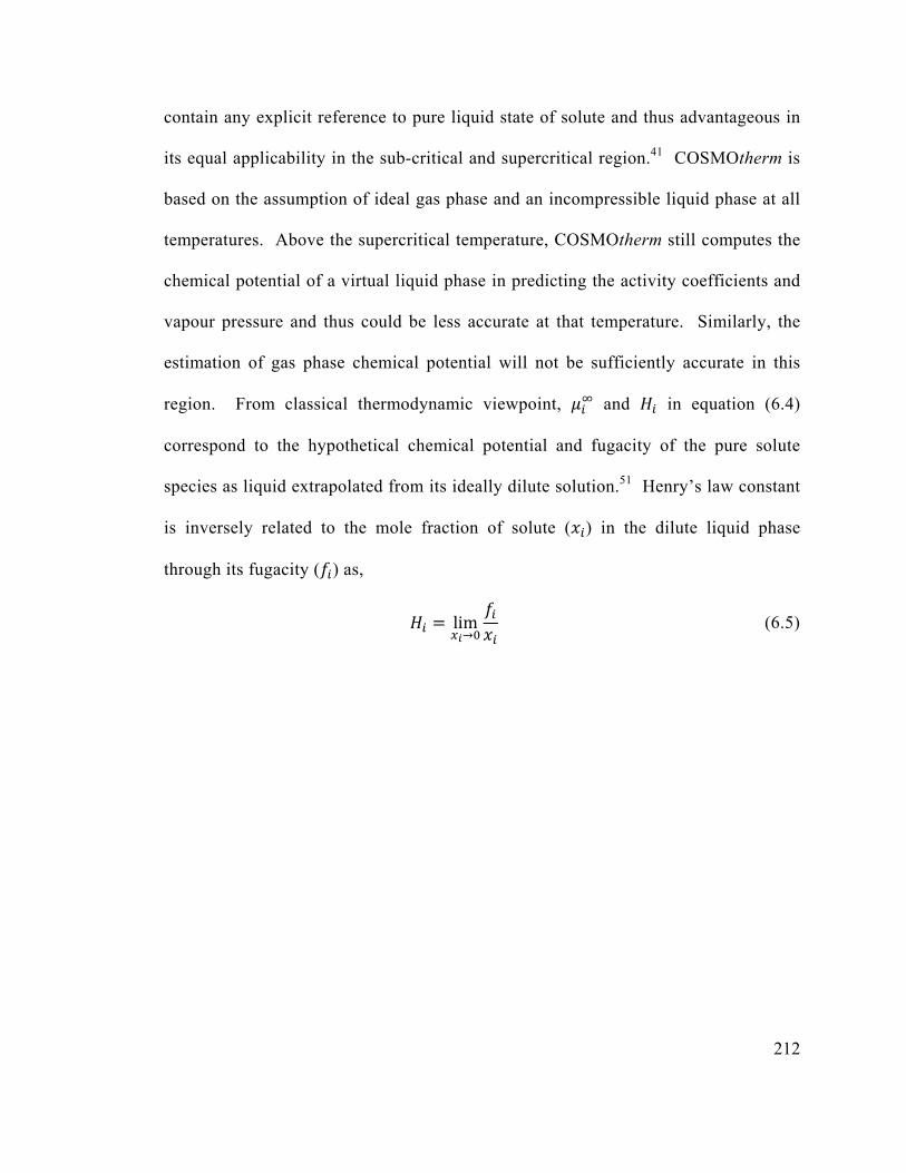
212

contain any explicit reference to pure liquid state of solute and thus advantageous in

its equal applicability in the sub-critical and supercritical region.41 COSMOtherm is

based on the assumption of ideal gas phase and an incompressible liquid phase at all

temperatures. Above the supercritical temperature, COSMOtherm still computes the

chemical potential of a virtual liquid phase in predicting the activity coefficients and

vapour pressure and thus could be less accurate at that temperature. Similarly, the

estimation of gas phase chemical potential will not be sufficiently accurate in this

region. From classical thermodynamic viewpoint, and in equation (6.4)

correspond to the hypothetical chemical potential and fugacity of the pure solute

species as liquid extrapolated from its ideally dilute solution.51 Henry’s law constant

is inversely related to the mole fraction of solute ( ) in the dilute liquid phase

through its fugacity ( ) as,

lim (6.5)

213

6.3 IL DATABASE AND COMPUTATIONAL DETAILS

The IL database used in this work consists of the ions available in the BP-

COSMO-IL database (obtained from COSMOlogic). COSMO calculations were

performed with the software TURBOMOLE52 using density functional theory (DFT)

level of theory, utilizing the Becke and Perdew functional53,54 with triple-zeta valence

polarized (TZVP) basis set.55. 73 cations and 37 anions were used to increase the

variation in anionic and cationic structure to facilitate trend analysis as well as to

increase the possibility of obtaining any fortuitous combination that may result in

practically useful IL for CO2 capture. For most cations, three conformers are used.

The list of the cations and anions with abbreviations, molecular weights, second

sigma moment56 of lowest energy conformer (sig2), a polarity descriptor (later

introduced in section 4.1.5), and an identification number (ID) used in this work are

given in Tables 6.1 and 6.2.

214

Table 6.1 List of Cations.

ID # Cation Abbreviation MW/(g/mol) N sig 2

1 3-methyl-imidazolium [mim] 83.11 20.27 113.382 1,3-methyl-imidazolium [mmim] 97.14 29.27 87.643 1-ethyl-3-methyl-imidazolium [emim] 111.17 29.74 84.964 1-butyl-3-methyl-imidazolium [bmim] 139.22 32.79 84.405 1-pentyl-3-methyl-imidazolium [C5mim] 153.25 34.22 84.896 1-hexyl-3-methyl-imidazolium [hmim] 167.27 35.70 85.387 1-heptyl-3-methyl-imidazolium [C7mim] 181.30 37.11 86.188 1-octyl-3-methyl-imidazolium [omim] 195.33 38.51 86.889 1-decyl-3-methyl-imidazolium [dmim] 223.38 41.38 88.22

10 1-dodecyl-3-methyl-imidazolium [C12mim] 251.43 44.19 89.6611 1-tetradecyl-3-methyl-imidazolium [C14mim] 279.49 47.03 91.2912 1-hexadecyl-3-methyl-imidazolium [C16mim] 307.54 49.91 92.8413 1-octadecyl-3-methyl-imidazolium [C18mim] 335.59 52.71 94.3614 1-butyl-imidazolium [bim] 125.19 23.78 109.9715 1-(2-hydroxyethyl)-3-methylimidazolium [OC2mim] 127.17 24.46 119.9716 1-benzyl-3-methyl-imidazolium [bnmim] 173.24 33.59 104.0717 3-methyl-1-(3-phenyl-propyl)-imidazolium [PhPrmim] 201.29 39.33 109.2318 1-ethyl-2-3-methyl-imidazolium [emmim] 125.19 31.13 77.0619 1-propyl-2-3-methyl-imidazolium [Prmmim] 139.22 32.70 76.4220 1-butyl-2-3-methyl-imidazolium [bmmim] 153.25 34.28 76.5821 1-hexyl-2-3-methyl-imidazolium [hmmim] 181.30 37.16 78.0322 1-hexadecyl-2-3-methyl-imidazolium [C16mmim] 321.57 51.33 85.2923 pyridinium [py] 80.11 19.09 116.7624 1-ethyl-pyridinium [epy] 108.16 30.26 84.9325 1-butyl-pyridinium [bpy] 136.22 33.17 83.7426 1-hexyl-pyridinium [hpy] 164.27 36.01 84.8927 1-octyl-pyridinium [opy] 192.32 38.87 86.2628 N-(3-hxdroxypropyl)pyridinium [PrOpy] 138.19 23.11 123.0729 N-(3-sulfopropyl)pyridinium [sppy] 202.25 25.91 195.8630 1-hexyl-3-methyl-pyridinium [hm(3)py] 178.30 37.05 78.4431 1-butyl-3-ethyl-pyridinium [be(3)py] 164.27 34.20 76.6532 1-butyl-3-methyl-pyridinium [bm(3)py] 150.24 33.52 77.3433 1-octyl -3-methyl-pyridinium [om(3)py] 206.35 39.86 79.8634 4-methyl-n-butylpyridinium [bm(4)py] 150.24 34.42 77.4335 1-hexyl-4-methyl-pyridinium [hm(4)py] 178.30 37.16 78.6336 4-methyl-1-octyl-pyridinium [om(4)py] 206.35 39.98 80.2937 1-butyl-3,4-dimethyl-pyridinium [bmm(4)py] 164.27 34.44 72.4738 1-butyl-3,5-dimethyl-pyridinium [bmm(5)py] 164.27 35.44 71.0639 1,1-dimethyl-pyrrolidinium [mmpyrr] 100.18 30.20 77.0440 1-ethyl-1-methyl-pyrrolidinium [empyrr] 114.21 30.20 73.4541 1-butyl-1-methyl-pyrrolidinium [bmpyrr] 142.26 33.10 72.7942 1-hexyl-1-methyl-pyrrolidinium [hmpyrr] 170.32 35.97 74.0243 1-octyl-1-methyl-pyrrolidinium [ompyrr] 198.37 38.68 75.4544 1,1-dipropyl-pyrrolidinium [dppyrr] 156.29 34.70 68.3645 1-butyl-1-ethyl-pyrrolidinium [bepyrr] 156.29 34.79 69.4046 1-(2-ethoxyethyl)-1-methylpyrrolidinium [EtOEtpyrr] 158.26 32.71 99.13

imid

azol

ium

pyri

dini

um/p

yrro

lidi

nium

215

Table 6.1 List of Cations (Continued)

ID # Cation Abbreviation MW/(g/mol) N sig 247 ammonium [NH4] 18.04 -3.09 196.1948 tetra-methylammonium [Me4N] 74.15 28.67 70.1449 tetra-ethylammonium [Et4N] 130.26 32.50 85.3050 tetra-n-butylammonium [Bu4N] 242.47 43.40 67.3151 ethyl-dimethyl-propylammonium [EtMe2PrN] 116.23 32.03 76.0252 methyl-trioctyl-ammonium [MeOc3N] 368.71 56.78 79.3753 bis(2-methoxyethyl)ammonium [(MeOEt)2N] 134.20 20.69 152.7754 ethyl-dimethyl-2-methoxyethylammonium [EDMA] 132.22 31.27 88.4855 dimethylethanolammonium [Me2EtOHN] 90.14 18.46 123.9656 diethanolammonium [(EtOH)2N] 106.14 9.07 169.3957 butyl-diethanolammonium [Bu(EtOH)2N] 162.25 21.26 135.9258 dodecyl-dimethyl-3-sulfopropylammonium [SPA] 336.56 40.24 193.1259 triisobutyl-methyl-phosphonium [(iBu)3MeP] 217.35 39.12 68.8160 tetrabutyl-phosphonium [Bu4P] 259.43 43.81 68.6061 trihexyl-tetradecyl-phosphonium [thtdP] 483.86 66.57 80.6962 benzyl-triphenyl-phosphonium [BnPh3P] 353.42 47.19 102.5663 guanidinium [G] 60.08 -2.79 162.3164 hexamethylguanidinium [Me6G] 144.24 33.12 58.4065 N,N,N,N-tetramethyl-N-ethylguanidinium [Me4EtG] 144.24 30.66 67.4466 N,N,N,N,N-pentamethyl-N-propyl-guanidinium[Me5PrG] 172.29 35.50 57.5967 N,N,N,N,N-pentamethyl-N-isopropyl-guanidini[Me5(iPr)G] 172.29 34.77 57.6368 O-methyl-N,N,N,N-tetramethylisouronium [O-Me4MeU] 131.20 32.93 72.1969 O-ethyl-N,N,N,N-tetramethylisouronium [O-Me4EtU] 145.22 34.20 70.1570 S-ethyl-N,N,N,N-tetramethylisothiouronium [S-Me4EtT] 161.29 31.88 67.3471 N-butyl-isoquinolinium [BuQ] 186.27 36.63 82.3872 1-(3-methoxypropyl)-1-methylpiperidinium [MeOPrMePi] 172.29 33.08 99.7673 aniline cation [C6H8N] 94.14 6.38 179.07

amm

oniu

m/p

hosp

honi

umot

her

cati

ons

216

Table 6.2 List of Anions.

ID # Anions Abbreviation MW/(g/mol) N sig 21 acetate [Ac] 59.04 -69.72 204.242 decanoate [NnCOO] 171.26 -57.51 207.363 benzoic acid anion [PhCOO] 121.11 -53.33 193.984 tetrafluoroborate [BF4] 86.80 -22.18 111.975 tetracyanoborate [B(CN)4] 114.88 1.27 102.806 bis- oxalatoborate [BOXB] 186.85 1.31 134.377 bis- malonatoborate [BMB] 214.90 -14.51 179.658 bis- salicylatoborate [BSB] 283.02 -12.54 167.869 bis- biphenyldiolatoborate [BPhB] 379.20 -0.60 173.55

10 methylsulfate [MeSO4] 111.10 -36.76 160.7011 ethylsulfate [EtSO4] 125.12 -36.71 163.3512 butylsulfate [BuSO4] 153.18 -33.69 163.4813 octylsulfate [OcSO4] 209.28 -29.49 166.6714 methoxyethylsulfate [MeOEtSO4] 155.15 -36.75 185.1415 ethoxyethylsulfate [EtOEtSO4] 169.18 -36.22 185.5116 2-(2-methoxyethoxy)ethylsulfate [MDEGSO4] 199.20 -37.93 211.2917 trifluoromethane-sulfonate [TfO] 149.07 -19.66 119.0718 toluene-4-sulfonate [TOS] 171.19 -41.81 187.6819 dicyanamide [DCA] 66.04 -28.70 132.9520 bis (trifluoromethyl)imide [BTI] 152.02 2.99 85.9921 bis (trifluoromethylsulfonyle)imide [Tf2N] 280.15 6.22 99.1022 Tricyanomethanide or cyanoform [(CN)3C] 90.06 -11.55 113.1823 bis (trifluoromethylsulfonyl)methane [Tf2C] 279.16 2.35 107.1624 tris (trifluoromethylsulfonyl)methide [Tf3C] 411.22 17.19 96.3925 dimethylphosphate [Me2P] 125.04 -62.04 209.8226 hexaflurophsophate [PF6] 144.96 3.78 88.1127 tris (pentafluoroethyl)trifluorophosphate [eFAP] 445.01 24.81 51.9728 tris (nonafluorobutyl)trifluorophosphate [bFAP] 745.06 43.50 54.2729 bis (2,4,4-trimethylpentyl)phosphinate [(Me3p)2PO2] 289.42 -49.98 210.4230 bis -pentafluoroethyl-phosphinate [(C2F5)2PO2] 301.00 -7.61 103.7431 chloride [Cl] 35.45 -72.15 189.3632 bromide [Br] 79.90 -55.52 170.5633 iodide [I] 126.90 -52.52 147.8534 chlorate [ClO4] 99.45 -12.21 113.0535 2-chlorophenol anion [2-PhCl] 127.55 -35.42 154.8536 3-chlorophenol anion [3-PhCl] 127.55 -36.97 154.7437 4-chlorophenol anion [4-PhCl] 127.55 -39.28 160.82

halo

geni

deac

etat

ebo

rate

sulp

hate

/sul

phon

ate

imid

e/am

ide

phos

phot

e/ph

inat

e

217

Both conventional usage and IUPAC conventions were given preference in

writing the abbreviations. For structural elucidation, cations used in this work are

grouped according to precursors like imidazolium, pyridinium, pyrrolidinium,

guanidinium, uronium, thiouronium, piperidinium and quinolinium; whereas anions

are classified into acetate, borate, imide/amide and methide, sulfate and sulfonate,

phosphate and phosphinate. The following ions in our database can also be found in

similar COSMO-based studies: cations with ID # {2-6,30,32,41,60,64,66,69,70},36

{3,4,8,18,20,21,25,30,32,59},37 {3,4,6,8,9,15,16,25,41,70},38,39

{3,4,6,8,48,49,50,60,61,64,66},41{3,4,6},42 and anions with ID#

{4,10,21,26,27},36{4,10,11,17,18,19,21,24,26},37 {1,4,10,17,19,21,26,27},38

{1,4,5,10,17,19,21,22,27,31},39 {4,17,19,21,22,25,26,34},41 {4,17,19,21,26}42.

All thermodynamic calculations are performed with COSMOtherm with the

C21-0108 parameterization.44 The mole fraction in solution is defined with respect to

the distinct ions. A binary mixture of an ionic liquid with a dissolved gas is thus

treated as a ternary solution. Therefore, the activity coefficients or the Henry’s law

constants obtained directly from COSMOtherm ( ) are converted to binary

framework by scaling them with 0.5, in order to make them comparable with

experimental results where the ionic liquid is considered as a single entity.57 The

vapour phase is assumed to be free of ionic liquids.

Selectivities are defined as / and / for CO2/CH4

and CO2/N2 separation where 1, 2, 3, and 4 in the subscripts indicate ILs, CO2, CH4

and N2 respectively and is the Henry’s law constant of solute in an ionic liquid

218

in the binary framework. The molar volumes of ionic liquids at 25°C were calculated

from the densities of ionic liquids which predicted by COSMOtherm.


Henry’s law constants of CO2 ( ) at 25°C and their relationship with

solvent properties and molecular interactions are discussed. Predicted at 25°C

and their quantitative evaluations are presented in sections 6.4.1 and 6.4.2. Trends in

due to structural variation are presented in section 6.4.3. The origin of these

trends in terms of solvent properties are discussed in section 6.4.4 and in terms of

activity coefficients in section 6.4.5. Effect of molar volume and polarity of ILs on

are discussed in section 6.4.6. Section 6.4.7 and 6.4.8 present solvation

properties of the three gases and selectivity.

6.4.1 Henry’s law constants at 25°C

Tables 6.3, 6.4 and 6.5 report Henry’s law constants of CO2 ( ) in 2701

ionic liquids. Table 6.3 reports in 814 imidazolium based ionic liquids (formed

from the 22 imidazolium cations and 37 anions). Di-substituted imidazolium cations

are arranged in order of increasing alkyl chain length which are followed by other

functional groups and tri-substituted cations. Table 6.4 reports in pyridinium and

pyrrolidinium based ionic liquids. Table 6.5 reports in ILs of precursors like

quinoline, piperidine, aniline and the non-ring cations such as ammonium,

phosphonium, guanidinium, thiouronium and isothiouronium..

219

Table 6.3 Henry's Law Constants of CO2 (bar) at 298.15 K in Imidazolium-Based Ionic Liquids

ID#

01_

[Ac]

ID#

02

_[N

nC

OO

]

ID#

03_[

Ph

CO

O]

ID#

04_

[BF

4]

ID#

05_

[B(C

N)4

]

ID#

06_[

BO

XB

]

ID#

07

_[B

MB

]

ID#

08_[

BS

B]

ID#

09_

[BP

hB

]

ID#

10_

[MeS

O4

]

ID#

11

_[E

tSO

4]

ID#

12_

[BuS

O4

]

ID#

13_

[OcS

O4

]

ID#

14

_[M

eO

EtS

O4]

ID#

15_

[EtO

EtS

O4

]

ID#

16

_[M

DE

GS

O4]

ID#

17_

[TfO

]

ID#

18_[

TO

S]

ID#

19

_[D

CA

]

ID#

20

_[B

TI]

ID#

21

_[T

f2N

]

ID#

22_

[(C

N)3

C]

ID#

23

_[T

f2C

]

ID#

24

_[T

f3C

]

ID#

25_

[Me2

P]

ID#

26_

[PF

6]

ID#

27_

[eF

AP

]

ID#

28_

[bF

AP

]

ID#

29

_[(M

e3p

)2P

O2

]

ID#

30_[

(C2

F5

)2P

O2

]

ID#

31

_[C

l]

ID#

32_

[Br]

ID#

33_

[I]

ID#

34

_[C

lO4]

ID#

35

_[2-

Ph

Cl]

ID#

36

_[3-

Ph

Cl]

ID#

37

_[4-

Ph

Cl]

ID# 01_[mim] 90 86 98 296 84 172 172 74 44 158 144 117 83 116 108 90 148 101 209 73 65 148 64 46 113 167 23 20 66 53 46 49 135 386 108 106 104

ID# 02_[mmim] 49 67 63 83 66 107 96 59 40 70 74 73 62 66 67 59 79 64 91 66 49 92 48 37 64 91 22 19 57 42 25 20 48 112 73 74 72

ID# 03_[emim] 57 64 60 71 55 84 81 52 37 66 67 64 56 60 60 53 64 58 79 49 42 73 42 34 63 62 21 19 55 38 39 29 60 93 64 65 64

ID# 04_[bmim] 65 60 58 61 46 66 70 47 34 65 62 58 51 57 55 50 53 54 68 37 36 58 36 30 63 44 20 18 53 34 61 42 73 78 57 57 57

ID# 05_[C5mim] 66 59 57 57 43 61 66 45 34 63 60 56 49 55 53 49 50 53 65 35 34 54 35 29 62 40 19 18 52 33 66 44 73 72 55 55 55

ID# 06_[hmim] 66 58 55 52 41 57 62 43 33 60 58 53 47 53 52 48 47 51 61 33 33 51 33 28 61 37 19 18 51 32 68 45 72 67 52 53 53

ID# 07_[C7mim] 66 56 54 49 39 54 59 42 32 58 56 52 46 52 50 47 45 50 58 31 32 49 32 28 60 35 19 18 50 31 70 45 70 62 51 51 52

ID# 08_[omim] 65 55 53 47 38 51 56 41 32 56 54 50 45 50 49 46 44 49 55 30 31 47 32 27 58 33 19 18 49 31 70 44 67 59 49 50 50

ID# 09_[dmim] 62 53 51 42 36 47 52 39 31 52 50 47 43 47 46 43 41 46 51 29 30 43 30 26 55 31 19 17 48 30 67 42 62 53 47 47 48

ID# 10_[C12mim] 59 51 49 39 35 44 48 37 30 49 47 45 41 45 44 42 39 44 48 28 29 41 30 26 53 29 19 17 47 29 64 40 58 49 45 45 46

ID# 11_[C14mim] 57 50 47 37 34 42 45 36 30 46 45 43 40 43 42 40 37 42 45 27 29 39 29 25 50 28 19 17 45 29 61 38 54 46 43 44 44

ID# 12_[C16mim] 55 48 45 35 33 40 43 35 29 44 43 41 39 41 40 39 36 41 44 27 28 38 28 25 48 27 19 18 44 28 58 36 51 43 42 42 43

ID# 13_[C18mim] 53 47 44 33 32 39 41 34 29 42 41 40 38 40 39 37 35 40 42 26 28 37 28 25 47 26 19 18 44 28 56 35 48 41 41 41 42

ID# 14_[bim] 100 75 76 99 55 89 98 56 38 101 91 78 63 80 75 67 74 73 100 42 44 77 45 35 91 58 20 19 61 40 115 84 134 129 70 70 70

ID# 15_[OC2mim] 71 75 76 120 74 115 111 64 42 95 94 87 70 82 80 70 92 77 118 67 53 105 53 40 82 99 24 20 61 46 47 40 86 152 83 83 82

ID# 16_[bnmim] 64 58 59 70 48 70 74 48 35 69 66 60 51 60 58 53 57 57 74 41 38 62 38 31 64 50 20 18 50 35 59 43 77 86 58 58 58

ID# 17_[PhPrmim] 56 51 50 52 41 57 60 42 32 55 53 50 44 50 48 45 46 48 58 34 33 50 33 28 54 39 19 17 45 31 55 38 62 65 49 50 49

ID# 18_[emmim] 44 53 47 47 46 66 63 45 33 49 50 50 46 47 47 43 48 46 56 40 36 55 36 30 48 45 20 18 48 32 31 20 43 64 51 52 51

ID# 19_[Prmmim] 48 52 47 46 42 59 59 42 32 49 49 48 44 46 46 42 45 45 55 35 34 51 34 29 49 39 19 18 47 31 39 24 49 62 49 50 50

ID# 20_[bmmim] 51 51 47 45 40 55 57 41 31 50 49 47 43 46 45 42 43 44 53 32 32 48 32 28 50 36 19 18 46 30 45 28 53 59 48 48 48

ID# 21_[hmmim] 54 50 47 42 37 49 53 38 30 49 47 45 41 44 44 41 40 43 50 29 30 44 30 27 50 32 19 18 45 28 53 32 55 54 45 46 46

ID# 22_[C16mmim] 48 43 40 31 31 37 39 33 27 39 38 37 35 37 36 35 33 36 39 25 27 34 27 24 43 25 19 18 40 26 49 29 44 39 38 38 39

halogenideim

ida

zoliu

m c

atio

ns

Anionsacetate borate sulfate & sulfonate imide/methide phosphate/phosphinate

220

Table 6.4 Henry's Law Constants of CO2 (bar) at 298.15 K in Pyridinium and Pyrrolidinium-Based Ionic Liquids

ID#

01

_[A

c]

ID#

02_

[NnC

OO

]

ID#

03_

[PhC

OO

]

ID#

04

_[B

F4]

ID#

05

_[B

(CN

)4]

ID#

06_[

BO

XB

]

ID#

07_

[BM

B]

ID#

08_

[BS

B]

ID#

09

_[B

PhB

]

ID#

10_

[Me

SO

4]

ID#

11

_[E

tSO

4]

ID#

12

_[B

uS

O4]

ID#

13

_[O

cSO

4]

ID#

14

_[M

eOE

tSO

4]

ID#

15

_[E

tOE

tSO

4]

ID#

16_

[MD

EG

SO

4]

ID#

17

_[T

fO]

ID#

18_

[TO

S]

ID#

19_

[DC

A]

ID#

20

_[B

TI]

ID#

21_

[Tf2

N]

ID#

22_

[(C

N)3

C]

ID#

23_

[Tf2

C]

ID#

24_

[Tf3

C]

ID#

25

_[M

e2P

]

ID#

26

_[P

F6]

ID#

27

_[e

FA

P]

ID#

28

_[b

FA

P]

ID#

29_

[(M

e3p

)2P

O2

]

ID#

30_

[(C

2F5)

2P

O2

]

ID#

31

_[C

l]

ID#

32

_[B

r]

ID#

33

_[I]

ID#

34

_[C

lO4

]

ID#

35

_[2

-PhC

l]

ID#

36

_[3

-PhC

l]

ID#

37

_[4

-PhC

l]

ID# 23_[py] 118 94 120 451 87 186 200 81 47 211 179 135 90 139 125 101 175 120 280 75 69 168 69 48 140 176 24 21 70 57 59 69 217 531 126 122 120

ID# 24_[epy] 61 68 66 84 59 91 89 56 39 75 75 71 59 66 65 58 72 64 90 56 45 81 45 35 69 72 22 19 57 40 41 32 68 107 71 71 70

ID# 25_[bpy] 71 64 62 67 47 69 73 49 36 70 67 62 53 60 58 53 57 58 74 40 38 62 38 31 67 48 20 19 55 35 66 48 80 84 61 61 61

ID# 26_[hpy] 72 61 59 57 42 59 65 45 34 64 61 57 49 56 54 50 50 55 65 34 34 54 35 29 65 39 20 18 53 33 75 52 78 70 55 56 56

ID# 27_[opy] 70 58 56 49 39 53 58 42 33 59 57 53 47 53 51 48 45 51 58 31 32 48 32 28 62 35 19 18 51 31 76 51 72 61 51 52 52

ID# 28_[PrOpy] 74 72 74 104 67 101 99 61 42 90 87 80 66 76 75 65 83 73 105 62 50 92 50 39 79 83 24 21 60 44 57 48 90 127 78 78 77

ID# 29_[sppy] 123 84 114 292 102 159 168 81 50 181 158 126 89 133 121 104 150 115 217 94 72 157 72 51 129 165 30 23 64 59 101 109 214 319 121 118 117

ID# 30_[hm(3)py] 59 53 50 44 38 51 55 40 32 52 50 47 43 47 45 43 42 46 53 31 31 46 31 27 53 33 19 18 48 30 60 37 60 57 48 49 49

ID# 31_[be(3)py] 59 55 52 49 41 57 60 43 33 54 53 50 45 49 48 44 46 48 58 34 33 51 34 29 55 38 20 18 49 32 55 35 61 64 51 52 52

ID# 32_[bm(3)py] 59 54 51 45 39 53 57 41 32 52 51 48 43 47 46 43 43 46 55 31 32 47 32 28 53 34 19 18 48 31 58 35 60 59 49 50 50

ID# 33_[om(3)py] 58 51 49 40 36 47 51 38 31 49 47 45 41 44 43 41 39 44 49 29 30 42 30 26 51 30 19 18 46 29 60 36 57 52 46 47 47

ID# 34_[bm(4)py] 59 55 52 49 41 57 60 43 33 54 53 50 45 49 48 44 46 48 58 34 33 51 34 29 55 37 20 18 49 32 56 35 61 64 52 52 52

ID# 35_[hm(4)py] 60 53 50 44 38 51 55 40 32 52 50 47 43 47 46 43 42 46 53 31 31 46 31 27 53 33 19 18 48 30 60 37 61 57 48 49 49

ID# 36_[om(4)py] 58 51 49 40 36 47 51 38 31 49 47 45 41 45 44 41 40 44 49 29 30 43 30 26 52 30 19 18 46 29 61 36 58 52 46 47 47

ID# 37_[bmm(4)py] 49 48 45 39 37 50 52 39 30 45 44 43 40 41 41 38 39 41 48 30 31 43 31 27 46 32 19 18 44 29 46 26 50 52 45 46 46

ID# 38_[bmm(5)py] 48 46 43 37 36 49 51 38 30 44 43 42 39 40 40 38 38 40 47 29 30 42 30 27 44 31 19 18 43 29 44 25 48 51 44 45 45

ID# 39_[mmpyrr] 38 61 50 50 57 85 74 50 35 50 56 59 54 52 54 49 54 51 63 48 39 70 39 32 51 57 19 17 53 33 19 13 34 74 59 61 59

ID# 40_[empyrr] 40 54 45 43 48 68 63 44 33 46 49 51 47 46 47 43 45 45 55 38 35 57 34 29 46 43 18 17 49 30 25 15 38 64 51 53 52

ID# 41_[bmpyrr] 50 52 46 43 41 57 58 40 31 49 48 47 43 45 45 42 41 43 53 31 31 49 31 27 49 35 18 17 47 28 42 24 52 62 48 49 48

ID# 42_[hmpyrr] 53 50 46 41 37 51 54 38 30 48 47 45 41 44 44 41 39 42 50 28 29 44 29 26 50 31 18 17 45 27 51 28 56 57 45 46 46

ID# 43_[ompyrr] 54 49 45 38 35 47 50 37 29 47 45 43 40 43 42 40 37 41 47 27 28 41 28 25 49 29 18 17 44 26 55 29 55 52 44 44 44

ID# 44_[dppyrr] 42 45 39 34 36 49 49 36 29 40 40 40 38 38 38 36 35 37 44 28 29 41 28 26 41 29 18 17 41 25 37 19 43 50 41 42 42

ID# 45_[bepyrr] 44 46 41 36 37 50 51 37 29 42 42 41 39 40 40 37 36 38 45 28 29 42 29 26 43 30 18 17 42 26 39 20 45 52 42 43 43

ID# 46_[EtOEtpyrr] 56 57 52 53 46 65 65 44 33 57 56 54 48 52 52 47 48 50 63 37 34 56 34 29 57 42 19 17 50 31 49 30 61 73 54 55 55

halogenide

Anionsacetate borate sulfate & sulfonate imide/methide phosphate/phosphinate

pyri

dini

um c

atio

nsp

yrro

lidin

ium

Ca

tions

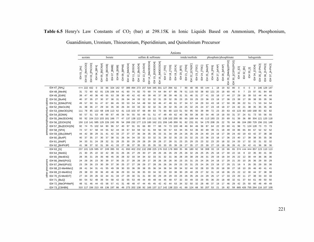
221

Table 6.5 Henry's Law Constants of CO2 (bar) at 298.15K in Ionic Liquids Based on Ammonium, Phosphonium,

Guanidinium, Uronium, Thiouronium, Piperidinium, and Quinolinium Precursor

ID#

01_[

Ac]

ID#

02_

[NnC

OO

]

ID#

03_[

PhC

OO

]

ID#

04_[

BF

4]

ID#

05_

[B(C

N)4

]

ID#

06_

[BO

XB

]

ID#

07_

[BM

B]

ID#

08_

[BS

B]

ID#

09_

[BP

hB

]

ID#

10_

[MeS

O4

]

ID#

11_

[EtS

O4]

ID#

12_

[BuS

O4]

ID#

13_[

OcS

O4]

ID#

14_[

MeO

EtS

O4

]

ID#

15_

[EtO

EtS

O4]

ID#

16_

[MD

EG

SO

4]

ID#

17_

[TfO

]

ID#

18_

[TO

S]

ID#

19_

[DC

A]

ID#

20_[

BT

I]

ID#

21_

[Tf2

N]

ID#

22_

[(C

N)3

C]

ID#

23_

[Tf2

C]

ID#

24_

[Tf3

C]

ID#

25_

[Me2

P]

ID#

26_[

PF

6]

ID#

27_

[eF

AP

]

ID#

28_

[bF

AP

]

ID#

29_

[(M

e3p)

2PO

2]

ID#

30_

[(C

2F

5)2

PO

2]

ID#

31_

[Cl]

ID#

32_

[Br]

ID#

33_

[I]

ID#

34_

[ClO

4]

ID#

35_

[2-P

hCl]

ID#

36_

[3-P

hCl]

ID#

37_

[4-P

hCl]

ID# 47_[NH4] 6774 222 432 0 33 66 324 142 57 389 494 273 157 544 345 301 127 394 62 7 90 48 95 65 1289 1 18 19 92 80 0 0 0 0 146 129 147

ID# 48_[Me4N] 31 72 60 62 81 135 106 64 41 60 74 82 70 69 74 64 84 67 86 78 51 115 50 38 60 121 20 18 60 40 9 7 23 97 81 84 80

ID# 49_[Et4N] 39 47 40 36 40 55 53 39 30 40 42 42 40 39 40 37 38 39 46 31 31 46 31 27 41 33 18 17 44 27 29 16 39 53 44 45 44

ID# 50_[Bu4N] 40 37 35 27 30 37 38 31 26 34 34 33 32 33 32 31 29 32 35 23 25 33 25 23 36 23 18 17 36 23 39 17 39 38 35 35 36

ID# 51_[EtMe2PrN] 49 57 50 51 47 67 66 45 33 53 54 54 48 50 50 46 47 48 61 37 34 57 34 29 53 43 18 17 50 30 36 22 51 71 53 54 54

ID# 52_[MeOc3N] 41 38 36 27 29 34 35 30 26 34 33 33 32 32 32 31 29 32 35 24 25 32 25 24 37 23 19 18 37 24 42 21 38 35 35 35 36

ID# 53_[(MeOEt)2N] 111 78 85 122 68 106 113 62 41 115 103 87 68 89 83 73 84 80 123 51 50 95 50 39 99 72 23 20 63 43 123 83 160 168 83 82 82

ID# 54_[EDMA] 50 57 51 53 49 69 67 46 34 54 55 55 49 51 51 47 49 49 62 40 36 59 36 30 54 46 19 18 50 31 37 24 51 73 55 56 55

ID# 55_[Me2EtOHN] 93 92 104 213 103 181 166 77 47 137 138 122 89 115 111 92 138 102 200 85 65 169 64 45 113 193 23 20 69 51 39 36 88 304 121 120 118

ID# 56_[(EtOH)2N] 150 110 141 585 129 226 243 95 54 269 232 177 115 180 162 131 206 145 359 91 82 231 81 54 170 208 26 22 78 64 86 104 280 729 156 151 148

ID# 57_[Bu(EtOH)2N] 92 74 75 102 64 90 96 57 40 97 91 81 66 80 77 68 74 73 103 48 46 84 46 36 87 64 22 20 60 41 96 71 124 128 73 73 73

ID# 58_[SPA] 72 57 57 58 44 55 62 44 34 67 64 59 52 61 59 56 50 57 63 34 35 53 36 30 69 39 21 18 49 33 86 65 84 67 52 52 52

ID# 59_[(iBu)3MeP] 44 42 38 29 31 41 42 33 27 37 37 36 34 35 35 33 31 34 39 24 26 35 26 24 40 24 18 17 39 24 43 19 43 42 37 38 38

ID# 60_[Bu4P] 40 37 35 27 30 37 38 31 26 34 34 33 32 33 32 31 29 32 35 23 25 32 25 23 36 23 18 17 36 23 40 17 39 38 35 35 36

ID# 61_[thtdP] 34 33 31 24 28 32 31 28 25 30 29 29 28 29 28 28 27 28 31 23 25 29 25 23 32 23 20 18 32 24 33 17 32 32 31 32 32

ID# 62_[BnPh3P] 41 38 37 32 31 39 41 33 27 38 37 35 33 35 35 33 33 35 39 26 27 35 27 25 39 27 19 18 36 26 41 24 42 41 36 36 36

ID# 63_[G] 237 101 126 595 87 249 395 93 41 650 402 232 132 288 225 176 310 176 369 35 96 180 92 58 308 33 19 19 66 65 374 1306 3858 857 123 110 113

ID# 64_[Me6G] 21 30 25 22 32 42 38 31 26 26 27 29 30 27 28 26 26 26 29 25 26 32 26 25 25 25 18 17 30 22 16 8 22 35 30 31 30

ID# 65_[Me4EtG] 28 35 31 29 35 48 45 35 28 32 33 34 34 32 33 31 32 31 36 28 29 38 29 26 31 29 19 18 34 25 22 12 30 44 36 36 36

ID# 66_[Me5(Pr)G] 24 29 26 23 30 39 37 30 25 27 28 28 29 27 28 26 26 26 30 23 25 31 25 24 26 24 18 17 29 21 20 10 26 36 29 30 29

ID# 67_[Me5(iPr)G] 23 29 26 23 30 39 37 30 25 27 27 28 29 27 28 26 26 26 29 23 25 31 25 24 26 23 18 17 29 21 19 9 26 35 29 30 30

ID# 68_[O-Me4MeU] 28 41 34 31 41 55 49 39 30 33 36 39 38 35 36 34 36 34 39 34 32 44 32 28 33 35 20 18 39 27 18 10 26 46 40 41 41

ID# 69_[O-Me4EtU] 29 38 33 30 36 49 46 36 29 33 34 36 35 33 34 32 33 33 38 30 29 40 29 27 32 31 19 18 36 25 22 12 30 44 37 38 38

ID# 70_[S-Me4EtT] 27 34 29 26 32 44 41 33 27 29 30 31 31 30 30 29 29 29 33 25 26 35 26 24 29 26 17 17 33 23 20 11 27 38 33 33 33

ID# 71_[BuQ] 60 54 52 48 39 54 58 42 32 55 53 49 44 49 48 44 45 48 57 32 33 49 33 29 55 36 20 18 48 32 61 37 64 61 49 50 50

ID# 72_[MeOPrMePi] 48 51 46 44 43 58 57 41 31 48 48 47 44 45 45 42 42 44 53 34 32 50 32 28 48 37 19 17 46 29 42 25 50 60 48 49 49

ID# 73_[C6H8N] 310 117 156 213 69 136 197 86 49 273 202 138 92 165 137 117 142 138 223 41 69 124 68 50 207 53 21 19 82 59 665 426 755 264 116 107 109

halogenideborate sulfate & sulfonate imide/methide phosphate/phosphinate

Anionsacetate

oth

er p

recu

rsor

sam

mon

ium

/ph

osph

oniu

m c

atio

ns

222

6.4.2 Quantitative evaluation of predicted HLC

Henry’s law constants around room temperature for 26 ILs are compared with

experimental data12,24,33,36,58-63 in Figure 6.1. The absolute average deviation and root

mean square deviation (defined below) are 15% and 9.1 respectively.

%1 100

(6.6)

1 (6.7)

Greater discrepancies appear in the prediction of [bmpyrr][eFAP], [S-

Me4EtT][eFAP], [thtdPh][Cl], [MeOc8N][Tf2N], [bmmim][BF4], [bmmim][PF6],

[bmim][MeSO4], [emim][EtSO4]. However, the deviations are within the overall

accuracy of the method and considering the fact that Henry’s law constant obtained

from experiment can vary to a large extent, the quantitative prediction can be

considered satisfactory. Rigorous evaluation of COSMOtherm prediction of gas

solubilities at different temperatures and pressures in ionic liquids was done by

Manan et al.37.

223

Figure 6.1 Comparison of Henry’s law constants of CO2: Predicted (grey); and

experimental (black).

0

1020

30

40

50

6070

80

90

100

[C5m

im][

bF

AP

](29

8.15

K)

[hm

im][

eFA

P](

298.

6K)

[MeO

c8N

][T

f2N

](30

3.15

K)

[bm

pyr

r][e

FA

P](

298.

6K)

[th

tdP

][D

CA

](30

3.15

K)

[S-M

e4E

tT][

eFA

P](

298.

6K)

[om

im][

Tf2

N](

298.

15K

)[h

mim

][T

f2N

](29

8.15

K)

[hm

py]

[Tf2

N](

298.

15K

)[b

mim

][T

f2N

](29

8K)

[th

tdP

][C

l](3

03.1

5K)

[em

im][

Tf2

N](

298.

15K

)[t

htd

P][

Tf2

N](

303.

15K

)[b

nm

im][

Tf2

N](

295K

)[b

mp

yrr]

[Tf2

N](

298K

)[e

mm

im][

Tf2

N](

298.

15K

)[b

mim

][P

F6]

(298

K)

[bm

im][

BF

4](2

98K

)[b

mm

im][

BF

4](2

98.1

5K)

[bm

mim

][P

F6]

(298

.15K

)[b

mim

][O

cSO

4](3

13.1

5K)

[em

im][

TfO

](30

3K)

[bm

im][

MeS

O4]

(293

.2K

)[e

mim

][D

CA

](30

3K)

[em

im][

BF

4](3

03K

)[e

mim

][E

tSO

4](3

03.3

8K)

H21

/ 0.1

MP

a

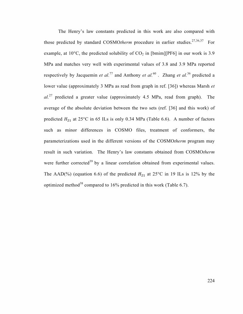
224

The Henry’s law constants predicted in this work are also compared with

those predicted by standard COSMOtherm procedure in earlier studies.27,36,37 For

example, at 10°C, the predicted solubility of CO2 in [bmim][PF6] in our work is 3.9

MPa and matches very well with experimental values of 3.8 and 3.9 MPa reported

respectively by Jacquemin et al.77 and Anthony et al.60 . Zhang et al.36 predicted a

lower value (approximately 3 MPa as read from graph in ref. [36]) whereas Marsh et

al.27 predicted a greater value (approximately 4.5 MPa, read from graph). The

average of the absolute deviation between the two sets (ref. [36] and this work) of

predicted at 25°C in 65 ILs is only 0.34 MPa (Table 6.6). A number of factors

such as minor differences in COSMO files, treatment of conformers, the

parameterizations used in the different versions of the COSMOtherm program may

result in such variation. The Henry’s law constants obtained from COSMOtherm

were further corrected39 by a linear correlation obtained from experimental values.

The AAD(%) (equation 6.6) of the predicted at 25°C in 19 ILs is 12% by the

optimized method38 compared to 16% predicted in this work (Table 6.7).

225

Table 6.6 Comparison of Henry’s law constants of CO2 Predicted in this Work with

those Predicted by Zhang et al. (2008) (Ref. 36).

Anions

[BF4]

(ID#4)

[PF6]

(ID#26)

[MeSO4]

(ID#10)

[Tf2N]

(ID#21)

[eFAP]

(ID#27)

Cations Ref.

36

This

work

Ref.

36

This

work

Ref.

36

This

work

Ref.

36

This

work

Ref.

36

This

work

[dmim] (ID#2) 64 83 86 91 72 70 49 49 23 22

[Emim](ID#3) 59 71 60 62 59 66 42 42 22 21

[Bmim](ID#4) 54 61 44 44 50 65 37 36 20 20

[pmim](ID#5) 51 57 40 40 47 63 35 34 20 19

[hmim](ID#6) 48 52 37 37 45 60 34 33 20 19

[bmpy](ID#32) 42 45 36 34 42 52 33 32 20 19

[hmpy](ID#30) 39 44 32 33 39 52 31 31 20 19

[bmpyrr](ID#41) 39 43 46 35 39 49 31 31 19 18

[HMG](ID#64) 21 22 25 25 27 26 26 26 19 18

[PPrG](ID#66) 22 23 24 24 26 27 25 25 19 18

[ETU](ID#69) 27 30 31 31 32 33 29 29 20 19

[ETT](ID#70) 20 26 23 26 24 29 23 26 17 17

[P(C4)4](ID#60) 25 27 23 23 27 34 25 25 20 18

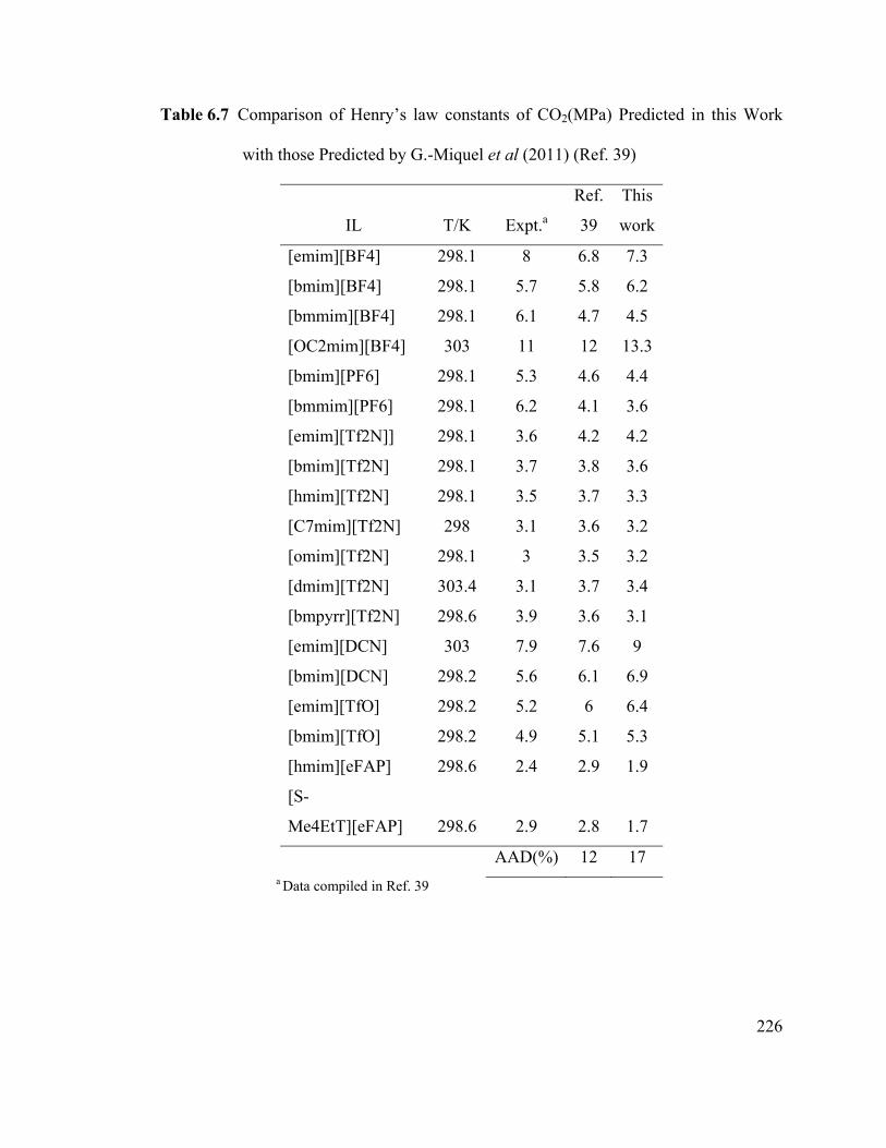
226

Table 6.7 Comparison of Henry’s law constants of CO2(MPa) Predicted in this Work

with those Predicted by G.-Miquel et al (2011) (Ref. 39)

IL T/K Expt.a

Ref.

39

This

work

[emim][BF4] 298.1 8 6.8 7.3

[bmim][BF4] 298.1 5.7 5.8 6.2

[bmmim][BF4] 298.1 6.1 4.7 4.5

[OC2mim][BF4] 303 11 12 13.3

[bmim][PF6] 298.1 5.3 4.6 4.4

[bmmim][PF6] 298.1 6.2 4.1 3.6

[emim][Tf2N]] 298.1 3.6 4.2 4.2

[bmim][Tf2N] 298.1 3.7 3.8 3.6

[hmim][Tf2N] 298.1 3.5 3.7 3.3

[C7mim][Tf2N] 298 3.1 3.6 3.2

[omim][Tf2N] 298.1 3 3.5 3.2

[dmim][Tf2N] 303.4 3.1 3.7 3.4

[bmpyrr][Tf2N] 298.6 3.9 3.6 3.1

[emim][DCN] 303 7.9 7.6 9

[bmim][DCN] 298.2 5.6 6.1 6.9

[emim][TfO] 298.2 5.2 6 6.4

[bmim][TfO] 298.2 4.9 5.1 5.3

[hmim][eFAP] 298.6 2.4 2.9 1.9

[S-

Me4EtT][eFAP] 298.6 2.9 2.8 1.7

AAD(%) 12 17 a Data compiled in Ref. 39

227

6.4.3 Trends in Henry’s law constant due to structural variations

To establish trends due to structural variations in the cations and anions,

in the model ionic liquids [cation][Tf2N] (represent 73 ILs) and [bmim][anion]

(represent 37 ILs) are used. Henry’s law constants of CO2, ; CO2/CH4

selectivity, ; CO2/N2 selectivity, ; residual activity coefficients at infinite

dilutions ( , ), enthalpy (∆ ) and entropy (∆S ) of solvation with their molar

volume(VIL),molecularweight (MWIL) and relative overall polarity parameter at

298.15K (NIL) are given in Table 6.8 for the 73 ionic liquids [cation][Tf2N] and in

Table 6.9 for the 37 ionic liquids [bmim][anion].

228

Table 6.8 Properties in the Ionic Liquids [cation][Tf2N]

Cations CO2 CH4 N2 CO2 CH4 N2 CO2 CH4 N2

ID#01_[mim] 363.3 0.220 26.49 65 16.5 37.7 -16.35 -3.55 -4.43 -89.5 -69.9 -79.7 -0.43 1.21 0.51ID#02_[mmim] 377.3 0.239 35.49 49 15.8 45.5 -16.78 -3.87 -3.84 -88.6 -68.2 -76.9 -0.69 0.91 0.44ID#03_[emim] 391.3 0.256 35.96 42 14.0 45.7 -17.13 -4.72 -4.12 -88.5 -68.9 -76.6 -0.82 0.66 0.32ID#04_[bmim] 419.4 0.290 39.00 36 11.6 44.9 -17.35 -5.70 -4.43 -88.0 -69.3 -76.3 -0.94 0.36 0.19ID#05_[C5mim] 433.4 0.307 40.44 34 10.8 44.6 -17.38 -6.00 -4.48 -87.7 -69.3 -76.0 -0.96 0.26 0.15ID#06_[hmim] 447.4 0.324 41.92 33 10.1 44.4 -17.40 -6.25 -4.51 -87.4 -69.3 -75.8 -0.99 0.17 0.13ID#07_[C7mim] 461.4 0.341 43.32 32 9.5 44.1 -17.38 -6.45 -4.53 -87.2 -69.2 -75.5 -1.00 0.10 0.11ID#08_[omim] 475.5 0.358 44.73 31 9.0 43.9 -17.37 -6.63 -4.53 -86.9 -69.2 -75.3 -1.01 0.04 0.09ID#09_[dmim] 503.5 0.392 47.60 30 8.2 43.5 -17.34 -6.91 -4.52 -86.5 -69.0 -74.9 -1.02 -0.07 0.08ID#10_[C12mim] 531.6 0.426 50.41 29 7.6 43.2 -17.30 -7.13 -4.50 -86.1 -68.8 -74.5 -1.02 -0.15 0.07ID#11_[C14mim] 559.6 0.460 53.25 29 7.1 42.9 -17.25 -7.30 -4.46 -85.7 -68.7 -74.1 -1.02 -0.21 0.06ID#12_[C16mim] 587.7 0.493 56.13 28 6.7 42.5 -17.19 -7.45 -4.42 -85.4 -68.5 -73.7 -1.01 -0.27 0.07ID#13_[C18mim] 615.7 0.527 58.93 28 6.3 42.2 -17.13 -7.57 -4.37 -85.1 -68.3 -73.4 -1.00 -0.31 0.07ID#14_[bim] 405.3 0.271 30.00 44 11.8 39.6 -17.05 -5.59 -4.83 -88.8 -70.8 -78.3 -0.74 0.56 0.25ID#15_[OC2mim] 407.3 0.261 30.68 53 14.3 39.9 -16.47 -4.01 -4.07 -88.3 -68.6 -77.4 -0.57 0.93 0.43ID#16_[bnmim] 453.4 0.303 39.81 38 12.6 52.6 -17.13 -4.96 -3.55 -87.7 -67.9 -75.0 -0.87 0.51 0.41ID#17_[PhPrmim] 481.4 0.337 45.55 33 11.7 54.6 -17.57 -5.60 -3.79 -88.0 -68.4 -75.0 -0.97 0.34 0.35ID#18_[emmim] 405.3 0.272 37.35 36 13.3 47.6 -17.59 -5.21 -4.22 -88.8 -68.8 -76.0 -0.96 0.47 0.22ID#19_[Prmmim] 419.4 0.290 38.92 34 12.2 46.9 -17.70 -5.67 -4.39 -88.6 -69.0 -75.9 -1.01 0.33 0.16ID#20_[bmmim] 433.4 0.307 40.50 32 11.2 46.4 -17.73 -6.00 -4.49 -88.3 -69.0 -75.8 -1.04 0.22 0.12ID#21_[hmmim] 461.4 0.341 43.38 30 9.9 45.5 -17.71 -6.45 -4.57 -87.7 -69.0 -75.4 -1.07 0.07 0.07ID#22_[C16mmim] 601.7 0.510 57.55 27 6.6 42.9 -17.43 -7.55 -4.49 -85.8 -68.3 -73.6 -1.05 -0.31 0.03ID#23_[py] 360.3 0.215 25.31 69 15.8 36.0 -16.17 -3.63 -4.54 -89.5 -70.3 -80.3 -0.36 1.23 0.53ID#24_[epy] 388.3 0.251 36.48 45 14.1 45.8 -16.87 -4.50 -3.94 -88.2 -68.7 -76.6 -0.76 0.73 0.38ID#25_[bpy] 416.4 0.285 39.39 38 11.6 45.2 -17.20 -5.59 -4.30 -87.8 -69.3 -76.3 -0.90 0.39 0.23ID#26_[hpy] 444.4 0.319 42.23 34 10.1 44.7 -17.27 -6.18 -4.42 -87.3 -69.3 -75.8 -0.96 0.20 0.16ID#27_[opy] 472.5 0.353 45.09 32 9.0 44.3 -17.28 -6.58 -4.45 -86.8 -69.2 -75.3 -0.99 0.05 0.12ID#28_[PrOpy] 418.3 0.273 29.32 50 13.2 41.5 -16.54 -4.43 -3.98 -88.0 -68.8 -76.8 -0.62 0.80 0.42ID#29_[sppy] 482.4 0.308 32.13 72 14.2 31.3 -15.57 -3.26 -4.39 -87.8 -68.6 -78.9 -0.22 1.28 0.54ID#30_[hm(3)py] 458.4 0.336 43.27 31 9.5 44.7 -17.54 -6.54 -4.56 -87.4 -69.3 -75.5 -1.03 0.06 0.09ID#31_[be(3)py] 444.4 0.312 40.42 33 10.8 45.5 -17.54 -6.09 -4.49 -88.0 -69.4 -76.0 -1.00 0.22 0.14ID#32_[bm(3)py] 430.4 0.309 39.74 32 10.1 44.9 -17.59 -6.37 -4.59 -87.8 -69.4 -75.8 -1.03 0.13 0.10ID#33_[om(3)py] 486.5 0.370 46.08 30 8.6 44.2 -17.50 -6.86 -4.58 -86.9 -69.1 -75.1 -1.05 -0.05 0.06ID#34_[bm(4)py] 430.4 0.303 40.63 33 10.7 45.4 -17.54 -6.10 -4.50 -88.0 -69.4 -76.0 -1.00 0.22 0.13ID#35_[hm(4)py] 458.4 0.336 43.38 31 9.5 44.7 -17.54 -6.54 -4.57 -87.4 -69.3 -75.5 -1.03 0.06 0.09ID#36_[om(4)py] 486.5 0.370 46.20 30 8.6 44.1 -17.49 -6.87 -4.58 -86.9 -69.2 -75.1 -1.04 -0.05 0.06ID#37_[bmm(4)py] 444.4 0.318 40.66 31 10.2 45.6 -17.79 -6.47 -4.64 -88.1 -69.4 -75.7 -1.07 0.09 0.07ID#38_[bmm(5)py] 444.4 0.320 41.66 30 10.0 45.3 -17.85 -6.56 -4.70 -88.2 -69.5 -75.8 -1.08 0.07 0.05ID#39_[mmpyrr] 380.3 0.253 36.42 39 15.6 45.7 -17.66 -4.62 -4.42 -89.7 -68.8 -77.0 -0.90 0.69 0.24ID#40_[empyrr] 394.4 0.269 36.42 35 14.1 45.8 -17.97 -5.30 -4.65 -89.7 -69.2 -76.8 -1.00 0.48 0.14ID#41_[bmpyrr] 422.4 0.303 39.32 31 11.8 44.8 -18.03 -6.05 -4.84 -89.0 -69.3 -76.4 -1.08 0.23 0.04ID#42_[hmpyrr] 450.5 0.337 42.19 29 10.3 44.1 -17.96 -6.47 -4.86 -88.3 -69.2 -75.9 -1.10 0.08 0.01ID#43_[ompyrr] 478.5 0.371 44.90 28 9.2 43.5 -17.88 -6.78 -4.84 -87.8 -69.0 -75.4 -1.10 -0.04 -0.01ID#44_[dppyrr] 436.4 0.317 40.92 29 11.0 44.9 -18.27 -6.47 -4.99 -89.1 -69.5 -76.2 -1.15 0.10 -0.02ID#45_[bepyrr] 436.4 0.319 41.01 29 11.0 44.7 -18.22 -6.42 -4.97 -89.0 -69.4 -76.2 -1.13 0.11 -0.01ID#46_[EtOEtpyrr] 438.4 0.309 38.93 34 12.2 44.6 -17.65 -5.61 -4.52 -88.6 -69.0 -76.2 -0.96 0.38 0.15ID#47_[NH4] 298.2 0.174 3.13 90 11.4 12.9 -17.44 -7.15 -10.17 -95.9 -81.7 -92.8 -0.17 1.09 -0.31ID#48_[Me4N] 354.3 0.237 34.89 51 18.3 44.7 -16.87 -3.24 -3.91 -89.2 -67.7 -77.4 -0.66 1.08 0.45ID#49_[Et4N] 410.4 0.299 38.72 31 12.4 46.0 -18.21 -6.00 -4.82 -89.5 -69.5 -76.5 -1.10 0.26 0.05ID#50_[Bu4N] 522.6 0.436 49.62 25 7.7 42.4 -18.11 -7.48 -5.06 -87.6 -69.0 -75.0 -1.17 -0.27 -0.09ID#51_[EtMe2PrN] 396.4 0.285 38.25 34 13.1 45.5 -17.81 -5.48 -4.60 -89.1 -69.2 -76.6 -1.00 0.42 0.14ID#52_[MeOc3N] 648.9 0.589 63.00 25 5.9 40.9 -17.52 -7.85 -4.66 -85.7 -68.1 -73.4 -1.05 -0.42 -0.01ID#53_[(MeOEt)2N] 414.3 0.285 26.91 50 12.1 35.0 -17.09 -5.23 -5.12 -89.9 -70.8 -79.3 -0.61 0.72 0.26ID#54_[EDMA] 412.4 0.293 37.48 36 13.2 44.8 -17.66 -5.30 -4.49 -89.0 -68.9 -76.4 -0.95 0.47 0.17ID#55_[Me2EtOHN] 370.3 0.241 24.68 65 16.3 34.3 -16.29 -3.26 -4.57 -89.3 -68.8 -79.4 -0.41 1.22 0.44ID#56_[(EtOH)2N] 386.3 0.249 15.29 82 14.7 26.9 -15.72 -3.34 -5.13 -89.4 -70.2 -81.2 -0.16 1.37 0.45ID#57_[Bu(EtOH)2N] 442.4 0.315 27.48 46 11.2 33.4 -16.83 -5.25 -5.04 -88.3 -69.5 -77.9 -0.67 0.59 0.16ID#58_[SPA] 616.7 0.495 46.46 35 8.3 36.1 -16.80 -6.39 -4.73 -86.0 -68.7 -75.3 -0.78 0.18 0.13ID#59_[(iBu)3MeP] 497.5 0.401 45.34 26 8.8 43.3 -18.14 -7.12 -5.03 -88.0 -69.1 -75.3 -1.17 -0.14 -0.08ID#60_[Bu4P] 539.6 0.447 50.03 25 7.7 42.4 -18.08 -7.48 -5.03 -87.5 -68.9 -74.9 -1.16 -0.28 -0.09ID#61_[thtdP] 764.0 0.717 72.79 25 5.2 39.9 -17.40 -8.14 -4.57 -85.1 -67.6 -72.7 -1.00 -0.51 0.02ID#62_[BnPh3P] 633.6 0.446 53.41 27 8.8 56.5 -17.63 -6.54 -3.55 -86.6 -67.5 -72.9 -1.06 -0.04 0.30ID#63_[G] 340.2 0.203 3.43 96 20.2 25.0 -15.77 -3.01 -5.81 -90.8 -73.0 -84.2 -0.07 1.78 0.46ID#64_[Me6G] 424.4 0.310 39.34 26 11.6 46.4 -18.93 -6.84 -5.31 -90.6 -70.4 -76.8 -1.25 0.04 -0.09ID#65_[Me4EtG] 424.4 0.307 36.88 29 11.3 44.6 -18.50 -6.62 -5.20 -90.0 -70.3 -77.0 -1.15 0.12 -0.03ID#66_[Me5PrG] 452.4 0.343 41.72 25 10.2 45.1 -18.82 -7.16 -5.35 -89.9 -70.1 -76.4 -1.26 -0.10 -0.13ID#67_[Me5(iPr)G] 452.4 0.341 40.99 25 10.5 45.3 -18.87 -7.11 -5.38 -90.1 -70.1 -76.5 -1.26 -0.07 -0.13ID#68_[O-Me4MeU] 411.3 0.286 39.15 32 13.0 44.9 -18.24 -5.72 -4.84 -89.9 -69.3 -76.6 -1.07 0.34 0.05ID#69_[O-Me4EtU] 425.4 0.304 40.42 29 11.9 45.4 -18.38 -6.21 -4.94 -89.8 -69.5 -76.4 -1.13 0.19 0.00ID#70_[S-Me4EtT] 441.4 0.311 38.10 26 12.7 49.8 -18.78 -6.36 -4.98 -90.1 -69.5 -76.3 -1.25 0.13 -0.02ID#71_[BuQ] 466.4 0.323 42.85 33 10.1 47.8 -17.37 -6.13 -4.15 -87.3 -68.9 -75.1 -0.99 0.17 0.20ID#72_[MeOPrMePi] 452.4 0.321 39.30 32 11.9 45.8 -17.89 -5.92 -4.61 -88.9 -69.4 -76.1 -1.01 0.31 0.13ID#73_[C6H8N] 374.3 0.235 12.60 69 11.0 29.5 -16.65 -5.69 -5.86 -91.0 -74.2 -83.0 -0.35 0.88 0.34

S23 S24H21/0.1

MPaVIL/(m3/

kmol)

MWIL/(g/

mol)NIL

imid

azol

ium

pyrid

iniu

m/p

yrro

lidin

ium

amm

oniu

m/p

hosp

honi

umot

her

catio

ns∆H∞(kJ/mol) ∆S∞(J/mol/K) ln γ ∞,r

229

Table 6.9 Properties in the Ionic Liquids [bmim][anion]

Cations CO2 CH4 N2 CO2 CH4 N2 CO2 CH4 N2

ID#01_[Ac] 198.3 0.193 -36.93 65 5.7 89.7 -16.85 -9.35 -2.25 -91.3 -80.5 -79.7 -0.47 0.09 1.33ID#02_[NnCOO] 310.5 0.327 -24.72 60 4.6 69.8 -15.33 -8.22 -1.45 -85.5 -74.4 -74.3 -0.39 -0.02 1.17ID#03_[PhCOO] 260.3 0.237 -20.55 58 6.9 108.4 -16.83 -7.98 -1.11 -90.2 -76.6 -76.4 -0.53 0.25 1.47ID#04_[BF4] 226.0 0.189 10.61 61 13.3 123.8 -16.71 -6.04 -0.39 -90.2 -76.0 -75.5 -0.54 0.88 1.59ID#05_[B(CN)4] 254.1 0.246 34.06 46 10.4 94.9 -16.42 -5.96 -1.05 -86.8 -71.2 -73.1 -0.76 0.42 1.11ID#06_[BOXB] 326.1 0.238 34.09 66 8.2 47.9 -15.84 -5.65 -2.35 -88.0 -71.2 -74.9 -0.38 0.56 0.81ID#07_[BMB] 354.1 0.269 18.27 70 8.3 67.7 -15.84 -6.23 -1.19 -88.4 -73.7 -74.3 -0.29 0.66 1.24ID#08_[BSB] 422.2 0.328 20.25 47 7.6 92.0 -16.37 -6.48 -0.53 -86.8 -70.6 -71.3 -0.62 0.25 1.22ID#09_[BPhB] 518.4 0.419 32.19 34 7.8 120.1 -17.16 -6.77 -0.27 -87.0 -69.2 -70.1 -0.84 0.06 1.27ID#10_[MeSO4] 250.3 0.209 -3.98 65 8.3 95.1 -16.60 -7.62 -1.18 -90.3 -77.7 -76.5 -0.45 0.49 1.41ID#11_[EtSO4] 264.3 0.226 -3.92 62 7.9 91.5 -16.37 -7.47 -1.09 -89.2 -76.5 -75.5 -0.47 0.43 1.36ID#12_[BuSO4] 292.4 0.259 -0.91 58 7.3 84.2 -16.08 -7.24 -1.05 -87.7 -74.6 -74.1 -0.50 0.33 1.25ID#13_[OcSO4] 348.5 0.327 3.29 51 6.5 75.1 -15.84 -7.21 -1.17 -85.8 -72.3 -72.5 -0.56 0.14 1.07ID#14_[MeOEtSO4] 294.4 0.253 -3.96 57 8.0 88.3 -16.69 -7.59 -1.41 -89.5 -76.3 -75.5 -0.53 0.39 1.26ID#15_[EtOEtSO4] 308.4 0.269 -3.43 55 7.7 85.2 -16.47 -7.42 -1.31 -88.6 -75.2 -74.7 -0.54 0.34 1.22ID#16_[MDEGSO4] 338.4 0.298 -5.14 50 7.8 84.3 -16.84 -7.68 -1.64 -89.1 -75.4 -75.0 -0.60 0.29 1.15ID#17_[TfO] 288.3 0.217 13.12 53 11.1 68.8 -16.78 -6.09 -2.54 -89.3 -73.4 -76.7 -0.64 0.61 0.91ID#18_[TOS] 310.4 0.267 -9.02 54 7.6 102.5 -16.53 -7.54 -0.88 -88.7 -75.3 -74.7 -0.55 0.32 1.40ID#19_[DCA] 205.3 0.197 4.08 68 9.0 115.5 -16.17 -6.81 -0.32 -89.4 -76.3 -75.7 -0.41 0.62 1.64ID#20_[BTI] 291.2 0.226 35.77 37 16.4 85.9 -17.90 -4.89 -2.54 -90.1 -69.7 -75.6 -0.98 0.65 0.78ID#21_[Tf2N] 419.4 0.290 39.00 36 11.6 44.9 -17.35 -5.70 -4.43 -88.0 -69.3 -76.3 -0.94 0.36 0.19ID#22_[(CN)3C] 229.3 0.220 21.23 58 9.7 110.0 -16.00 -6.05 -0.12 -87.4 -73.0 -73.3 -0.55 0.56 1.47ID#23_[Tf2C] 418.4 0.295 35.14 36 11.6 48.5 -17.34 -5.72 -4.15 -88.0 -69.4 -76.1 -0.92 0.37 0.28ID#24_[Tf3C] 550.4 0.356 49.98 30 11.3 36.7 -17.71 -5.83 -5.37 -87.7 -68.0 -76.3 -1.05 0.22 -0.12ID#25_[Me2P] 264.3 0.237 -29.25 63 6.3 85.9 -16.36 -8.50 -1.69 -89.3 -78.2 -77.1 -0.45 0.22 1.31ID#26_[PF6] 284.2 0.212 36.56 44 17.7 108.7 -17.45 -4.51 -1.03 -90.0 -70.5 -73.9 -0.84 0.87 1.16ID#27_[eFAP] 584.2 0.371 57.59 20 14.4 45.9 -19.31 -6.23 -6.27 -89.5 -67.8 -77.5 -1.48 0.03 -0.33ID#28_[bFAP] 884.3 0.529 76.29 18 12.9 34.2 -18.96 -6.30 -6.88 -87.7 -66.5 -76.5 -1.43 -0.02 -0.57ID#29_[(Me3p)2PO2] 428.6 0.452 -17.20 53 4.2 62.9 -15.18 -8.12 -1.46 -83.9 -72.1 -72.3 -0.42 -0.15 1.04ID#30_[(C2F5)2PO2] 440.2 0.304 25.18 34 11.4 45.7 -17.40 -6.21 -4.88 -87.6 -70.3 -77.4 -0.99 0.29 0.15ID#31_[Cl] 174.7 0.161 -39.36 61 5.4 89.6 -17.10 -10.48 -3.16 -91.6 -83.4 -82.2 -0.57 -0.06 1.22ID#32_[Br] 219.1 0.163 -22.74 42 9.9 143.9 -17.85 -9.77 -2.70 -90.9 -82.8 -81.4 -0.95 0.16 1.32ID#33_[I] 266.1 0.167 -19.73 73 7.3 112.3 -16.53 -8.60 -1.51 -91.1 -81.0 -80.0 -0.38 0.43 1.64ID#34_[ClO4] 238.7 0.187 20.58 78 9.5 76.2 -16.31 -6.18 -1.00 -90.9 -75.7 -75.6 -0.29 0.80 1.35ID#35_[2-PhCl] 266.8 0.228 -2.63 57 7.9 101.6 -16.91 -7.13 -1.18 -90.3 -74.7 -76.0 -0.54 0.36 1.39ID#36_[3-PhCl] 266.8 0.228 -4.19 57 7.6 95.4 -16.83 -7.10 -1.33 -90.1 -74.4 -76.0 -0.53 0.34 1.34ID#37_[4-PhCl] 266.8 0.228 -6.50 57 7.5 94.4 -16.90 -7.23 -1.44 -90.4 -74.7 -76.3 -0.54 0.32 1.33

MWIL/(g/

mol)VIL/(m3/

kmol)NIL

H21/0.1

MPaS23 S24

hal

ogen

ide

ace

tate

bora

tesu

lph

ate/

sulp

hona

teim

ide/

amid

eph

osph

ote/

phin

ate

∆H∞(kJ/mol) ∆S∞(J/mol/K) ln γ ∞,r

230

The cation [bmim] is regarded as a model cation for the analysis of structural

variations in the ring cations. Structural modifications relative to [bmim] that

enhance CO2 solubility (decrease ) include (i) increase in the alkyl chain lengthin

ring-precursor (ii) alkylation of ammonium and phosphonium cation

([Et4N][Tf2N]<[Bu4N][Tf2N] and [(iBu)3MeP][Tf2N<[Bu4P][Tf2N]), (iii) change

in cation family (e.g., for ring cation:[bmim] [Tf2N] <[bm(3)py][Tf2N]<[bmpyrr]

[Tf2N] and for non-ring cation: [O-Me4EtU]~[Me4EtG]<[S-Me4EtT], (iv)

substitution of methyl group in C2 position (e.g., [bmim][Tf2N]<[bmmim][Tf2N]).

Cation modifications that diminish CO2 solubility include the presence of the

following groups: hydroxyl (e.g., [bmim][Tf2N]>[OC2mim][Tf2N]), phenyl

([hmim][Tf2N]>[bnmim][Tf2N]), and ether ([bepyrr]][Tf2N]>[EtOEtpyrr]][Tf2N]).

Zhang et al. [36] showed that COSMO-RS predicts a reduction of CO2 solubility due

to the presence of electronegative fluorine in the cation. In general, the effect of

cation modification on is rather low. in the IL [cation][Tf2N] is around 3MPa

except some extreme cases (e.g., [NH4], [G], [mim], [Py] that may result in solid ILs

at room temperature when paired with relatively small anions).

Anions are less amenable to systematic structural variation but usually have

larger impact on gas solubility as can be seen from the large variation in the

magnitude of in Table 6.9 (1.8 to 7.8 MPa). Presence of fluorine-containing

anions results in smaller . Acetate, chloride, some large borate, dimethyl

phosphate, dicyanamide anions result in high (~6MPa) when paired with [bmim]

cation. Longer alkyl chain length generally enhances CO2 solubility

([bmim][MeSO4]<[bmim][OcSO4]; [bmim][Ac]<[bmim][NnCOO]). The presence

231

of ether group causes slight increase in the solubility of

CO2([bmim][BuSO4]<[bmim][MeOEtSO4]). Among the seven sulphate anions

considered, [MDEGSO4] has the lowest . Presence of hydroxyl group also results

in high Henry’s law constant as shown for the case of [bmim][Lactate] (6.2 MPa).36

The dominance of cation can be dramatically influenced by some anions. For

example, Tables 6.3, 6.4 and 6.5 reveal that all ILs with fluoroalkylphosphate (FAP)

anions have very similar indicating negligible effect of companion cations. On

the other hand, in ILs with chloride/bromide anion is highly influenced by the

counterpart cation. For example, in [O-Me4EtU][Br] and [dmim][Br] are (1.2

and 4.2) MPa respectively.

Comparison with experimental trends shows that COSMOtherm accurately

predicts the effect of alkyl chain length, phenyl and ether group in the cations relative

to the model [bmim] cation. However, its prediction is opposite to experimental

trend for the effect of methyl substitution on the C2 position of an imidazolium ring

and cation family.37 Cation fluorination was found59 to increase CO2 solubility

slightly but the COSMOtherm prediction shows the opposite trend36. For the [bmim]

cation, COSMOtherm predicts the correct order of the five anions as shown in Figure

6.1, i.e. [MeSO4]<[BF4]<[OcSO4]<[PF6]<[Tf2N]. In phosphonium ILs,

COSMOtherm incorrectly predicts the ordering between [thtdP][Cl] and

[thtdP][DCA] but correctly predicts that CO2 is less soluble in both of these ILs than

[thtdP][Tf2N]. COSMOtherm correctly predicts that increased fluorination on the

anion enhances CO2 solubility. Manan et al.37 found that COSMOtherm ordering of

five anions (nitrate<[BF4]<[TfO]<[PF6]<[Tf2N]) matched with experimental results

232

except the order between [PF6] and [TfO].

6.4.4 Qualitative interpretations of molecular interactions

The above mentioned trends in solubility are a consequence of the variations

in molecular interactions of ILs with CO2 which originate from the variations in the

chemical constituents, shapes and sizes of ILs. Effect of structural variations in the

ILs can be visualized through their sigma profiles. Corresponding sigma-potentials

of the solvents can be used to ascertain the affinity of solvents to a solute [24]. The

sigma profiles of four imidazolium cations ([bmim], [bnmim], [omim] and

[OC2mim]) paired with [Tf2N] anion along with CO2 and CH4 are shown in Figure.

6.2.

Effect of benzyl, hydroxyl and alkyl chain length. The sigma profiles of the

ILs shown in Figure 6.2 extend from (+2 to -2) e/nm2. The similarity of the IL sigma

profiles within the range (0.5 to 2) e/nm2 is due to the common imidazolium ring and

within the range (-1 to -2) e/nm2is due to the common [Tf2N] anion. Major

differences among them are found around the neutral regions. Of the four ILs,

[omim][Tf2N], which has the highest CO2 solubility, is seen to have a lot more

nonpolar surfaces than others where sigma is 0e/nm2. Due to the apolar and

symmetric benzyl ring, [bnmim][Tf2N] is seen to have slightly more surfaces around

-0.7e/nm2 and 0.7 e/nm2. [OC2mim][Tf2N] has slightly more polar surface pieces

due to the polar oxygen at sigma +1.4 e/nm2. All four ILs have enough negative

surface pieces that will interact favourably with the positive surface pieces of CO2.

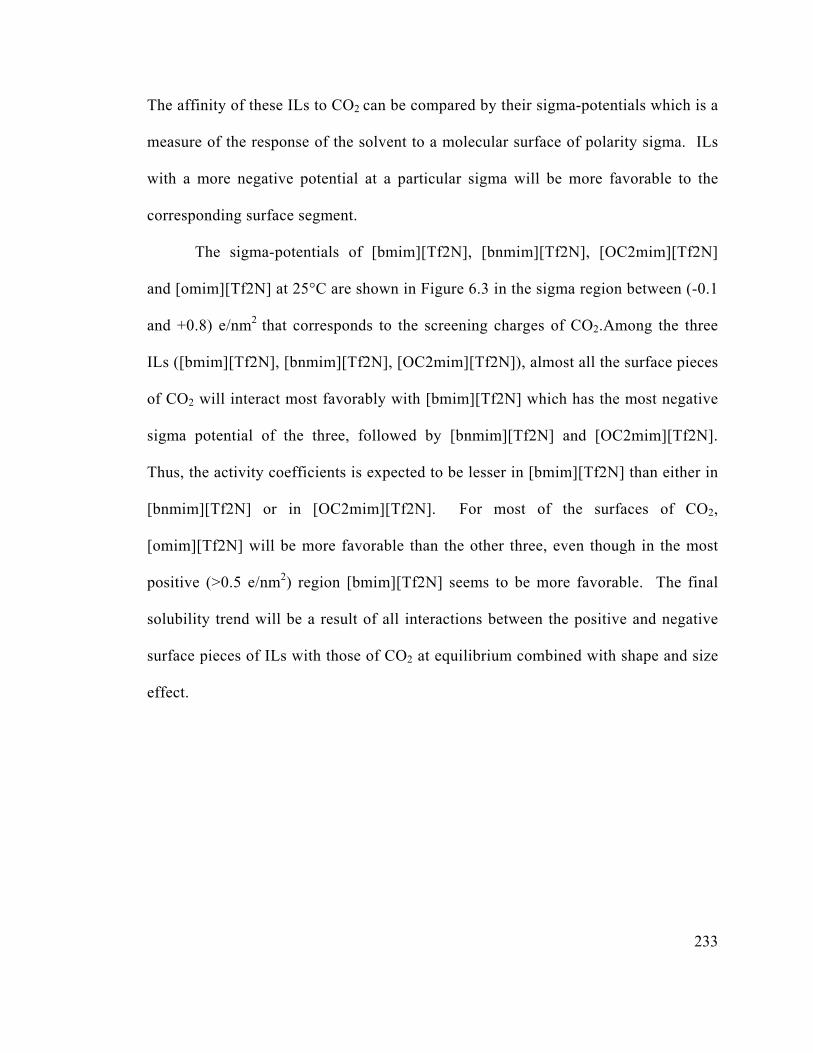
233

The affinity of these ILs to CO2 can be compared by their sigma-potentials which is a

measure of the response of the solvent to a molecular surface of polarity sigma. ILs

with a more negative potential at a particular sigma will be more favorable to the

corresponding surface segment.

The sigma-potentials of [bmim][Tf2N], [bnmim][Tf2N], [OC2mim][Tf2N]

and [omim][Tf2N] at 25°C are shown in Figure 6.3 in the sigma region between (-0.1

and +0.8) e/nm2 that corresponds to the screening charges of CO2.Among the three

ILs ([bmim][Tf2N], [bnmim][Tf2N], [OC2mim][Tf2N]), almost all the surface pieces

of CO2 will interact most favorably with [bmim][Tf2N] which has the most negative

sigma potential of the three, followed by [bnmim][Tf2N] and [OC2mim][Tf2N].

Thus, the activity coefficients is expected to be lesser in [bmim][Tf2N] than either in

[bnmim][Tf2N] or in [OC2mim][Tf2N]. For most of the surfaces of CO2,

[omim][Tf2N] will be more favorable than the other three, even though in the most

positive (>0.5 e/nm2) region [bmim][Tf2N] seems to be more favorable. The final

solubility trend will be a result of all interactions between the positive and negative

surface pieces of ILs with those of CO2 at equilibrium combined with shape and size

effect.

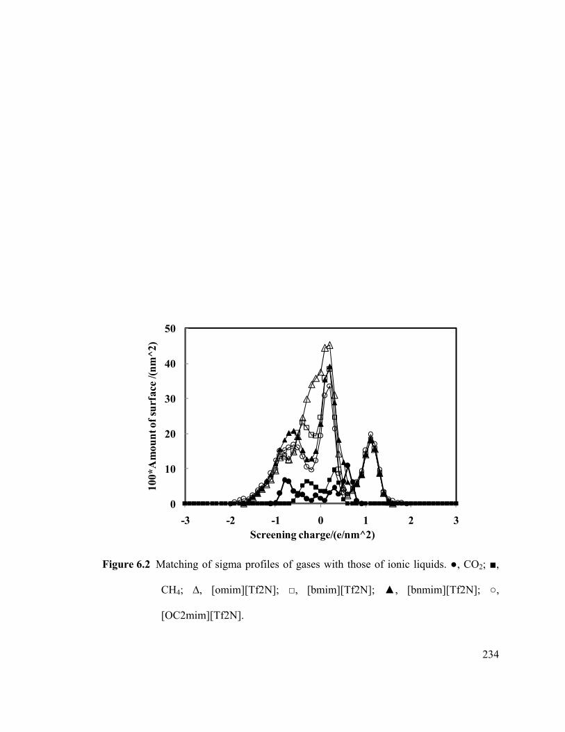
234

Figure 6.2 Matching of sigma profiles of gases with those of ionic liquids. ●, CO2; ■,

CH4; ∆, [omim][Tf2N]; □, [bmim][Tf2N]; ▲, [bnmim][Tf2N]; ○,

[OC2mim][Tf2N].

0

10

20

30

40

50

-3 -2 -1 0 1 2 3

100*

Am

oun

t of

surf

ace

/(n

m^

2)

Screening charge/(e/nm^2)

235

Figure 6.3 Sigma-potentials of ionic liquids with different alkyl chain length.: ○,

[OC2mim][Tf2N]; ▲, [bnmim][Tf2N]; □, [bmim][Tf2N]; ∆,

[omim][Tf2N].

-8

-6

-4

-2

0

2

4

-1 -0.8 -0.6 -0.4 -0.2 0 0.2 0.4 0.6 0.8

µ(σ

)/(k

J/m

ol/n

m2 )

Screening charge, σ/(e/nm2)

236

Effect of C2 substitution and change in cation family. Sigma-potentials of

[bmim][Tf2N], [bmmim][Tf2N], [bm(3)py][Tf2N] and [bmpyrr][Tf2N] are shown in

supplementary information (Figure 6.4). The sigma-potentials of [bmim][Tf2N] and

[bmmim][Tf2N] reveal that substitution of acidic hydrogen in the C2 position of the

imidazolium ring with a more basic methyl group increase the affinity of the ionic

liquids towards CO2. Similarly, among the three ring cations with same alkyl chain

length, the affinity increases in the following order

[bmpyrr]>[bm(3)py]>[bmim].Sigma-potentials of phosphonium and ammonium

cation with same alkyl chain length, [Bu4P][Tf2N] and [Bu4N][Tf2N], in the sigma

region (-0.1 and +0.8) e/nm2 are identical (Figure 6.5) indicating similar degree of

interaction; and therefore, the trend between these two cations will be determined by

shape and size effect. The difference between the guanidinium, uranium and

thiouronium cation based ILs with [Tf2N] are also small, the thiouronium cation will

have slightly more affinity toward CO2 (Figure 6.5).

237

Figure 6.4 Sigma-potentials of ionic liquids with different ring precursors: □,

[bmim][Tf2N]; ○, [bm(3)py][Tf2N]; ∆, [bmmim][Tf2N]; ▲,

[bmpyrr][Tf2N].

-8

-6

-4

-2

0

2

4

-1 -0.8 -0.6 -0.4 -0.2 0 0.2 0.4 0.6 0.8

µ(σ

)/(k

J/m

ol/n

m2 )

Screening charge, σ (e/nm2)

238

Figure 6.5 Sigma-potentials of ionic liquids with non ring precursors: □, [bmim][Tf2N];

○, [Bu4P][Tf2N]; ∆, [Bu4N][Tf2N]; ▲, [Me4EtG][Tf2N]; ■, [O-

Me4EtU][Tf2N]; ●, [S-Me4EtT][Tf2N].

-10

-8

-6

-4

-2

0

2

4

-1 -0.8 -0.6 -0.4 -0.2 0 0.2 0.4 0.6 0.8

µ(σ

)/(k

J/m

ol/n

m2 )


239

Effect of anions. The differences between the sigma-potentials of ionic

liquids are much more pronounced when different anions are paired with a same

cation as can be seen in Figure 6.6. Among the ILs shown, [bmim][EtSO4] will

favour the surfaces having charge (0 to 0.8) e/nm2, but disfavours the surfaces with

charge (-0.2 to -1) e/nm2. The final solubility will be the result between the two

competing effects at equilibrium. Due to these competitive effects, it is more

difficult to categorize the anion effect through their sigma-potentials.CO2 has the

highest solubility in ILs containing FAP anions which has negative sigma potential

within the whole range of CO2 sigma charge. The reason for the high miscibility of

CO2 with FAP anions can also be explained by the complementarity of the sigma

profiles of [bmim][eFAP] and CO2 shown in Figure 6.7. Almost all the surface

pieces of CO2will find opposite surface pieces when dissolved in [bmim][eFAP] and

thus will have low misfit energy. The sigma profile of [bmim][Cl] is also shown in

Figure 6.7. Since halogens lie in the extreme polar regions, slight difference in

polarity results in significant difference in misfit energy and hydrogen-bonding

among the surface pieces of ionic liquids and thus making the mixture environment

very different in different ILs.

240

Figure 6.6 Sigma-potentials of ionic liquids with different anions: ●, [bmim][BF4]; ∆,

[bmim][DCA]; □, [bmim][Tf2N]; ▲, [bmim][EtSO4]; ■, [bmim][eFAP];

○, [bmim][TfO].

-10

-8

-6

-4

-2

0

2

4

6

8

10

-1 -0.8 -0.6 -0.4 -0.2 0 0.2 0.4 0.6 0.8

µ(σ

)/(k

J/m

ol/n

m2 )


241

Figure 6.7 Comparison of CO2 sigma profiles with those of some ionic liquids: ●, CO2;

□, [bmim][Tf2N]; ▲, [bmim][eFAP]; ○, [bmim][Cl].

0

10

20

30

40

50

60

70

-3 -2 -1 0 1 2 3

100*

Su

rfac

e A

rea

/(n

m^

2)

Screening charges, σ/(e/nm^2)

242

6.4.5 Activity coefficients at infinite dilutions

Activity coefficients are useful quantitative means for studying the solubility

of single gas in different solvents. According to equation 6.2, trends in Henry’s law

constants are identical to the trends in as the vapour pressure of solute remains

same. The activity coefficient of a solute in a mixture is a measure of the degree of

non-ideality in the liquid mixture with reference to its pure liquid state. The residual

chemical potential ( , ) reflects non-ideality due to energetic interactions, and was

obtained by switching off the combinatorial contributions for all compounds. ln , ,

that reflects non-ideality due to solute-solvent size and shape differences, is defined

to be the difference between ln and ln , . These quantities for CO2, CH4 and N2

in the model ionic liquids are given in Tables 6.10 and 6.11 to show the effect of

structural variation in cations and anions. Henry’s law constants can be expressed in

terms of these quantities as,

, , (6.10)

According to the above equation, more negative values of ln , and ln ,

tend to decrease Henry’s law constants. These values are all negative for CO2. The

ln , of CO2 in [OC2mim][Tf2N], [bnmim][Tf2N], [bmim][Tf2N], [omim][Tf2N]

are (-0.84, -1.18, -1.23, -1.37) and consistent with our discussions in section 6.4.3

(Qualitative interpretations of molecular interactions). Among the anions, ln ∞, is

more negative in case of fluorine-containing anions. Since the screening charge of

243

CO2 lies in the electrostatic misfit region, attempt is made to correlate , with the

electrostatic polarity, quantified as second sigma moment (sig2)56, of the varying ions

for a fixed counterpart ion. The trend is not linear and, in general, activity

coefficients seem to increase with increase in sig2 (Figures 6.8 and 6.9). For

example, among the anions, the FAP anions has the lowest sig2 values that results in

smaller values of residual activity coefficients, and consequently in low .

However, there are a lot of exceptions to this relationship that undermines the

significance of sig2 as a tool for solvent characterization.

244

Figure 6.8 Effect of electrostatic polarity, sig2, of cations on residual activity

coefficients of CO2 in the ILs [cation][Tf2N].

Figure 6.9 Effect of electrostatic polarity, sig2, of anions on residual activity

coefficients of CO2 in the ILs [bmim][anion].

0.0

0.1

0.2

0.3

0.4

0.5

0.6

0.7

0.8

0.9

1.0

0 100 200 300Res

idua

l act

ivit

y co

effic

ient

of C

O2

in

[cat

ion]

[Tf2

N]

Electrostatic polarity (sig2) of cationsin the ILs [cation][Tf2N]

0.0

0.1

0.2

0.3

0.4

0.5

0.6

0.7

0.8

0.9

1.0

0 100 200 300Res

idua

l act

ivit

y co

effic

ient

of C

O2

in

[bm

im][

anio

n]

Electrostatic polarity (sig2) of anions in the ILs [bmim][anion]

245

The values of ln ∞, are negative for the three gases which favors their

solubility as per equation 6.3. Since the combinatorial contribution ln ∞, reflects

the difference of area and volume of an ionic liquid with those of the solute, it may

be correlated with a size parameter of the solvent. For example, ∞, of CO2 was

correlated with molar volume of the IL with the relationship ∞, 0.22

0.467 with a correlation coefficient 0.99 where represents the molar volume

(m3/kmol) (Figure 6.10). Prediction of activity coefficients of some liquid solutes in

ionic liquids using COSMO-RS was found satisfactory.57

246

Figure 6.10 Effect of molar volume on the combinatorial activity coefficients of CO2 in

the ILs [bmim][anion] and [cation][Tf2N].

0.5

0.6

0.7

0.8

0.9

1.0

0.0 0.2 0.4 0.6 0.8Com

bin

ator

ial A

ctiv

ity

Coe

ffic

ein

t at

infi

nit

e d

iluti

on o

f C

O2

in I

Ls

[bm

im][

anio

n]

and

[cat

ion

][T

f2N

]

Molar Volume of ILs (m3/kmol)

247

6.4.6 Effect of molar volume and polarity on Henry’s law constant

Molar volume and polarity of ionic liquids are used in the literature to

correlate or explain the solubility of CO2 in ILs. For example, in predictive models

based on regular solution theories, Henry’s law constant of gases are correlated with

molar volume of solvent through the solubility parameters.12,64 According to scaled

particle theory,65 Henry’s law constant of a gas should decrease with increase in

molar volume of ILs when the cavity work and gas-liquid interaction remains same.

This implies that in ILs could be correlated with molar volume when a cation is

varied with a fixed anion as the effect of anion is more pronounced than that of a

cation on the gas-liquid interactions. On the other hand, the polarity, a key property

of a solvent, reflects the overall solvation capability due to varieties of solute-solvent

interactions and used often to characterize solvents.66 Bara et al.67 discussed the

effect of polarity of oligo(ethylene glycol)-functionalized imidazolium ionic liquids

on solubility and selectivity. Solvation of nonpolar, polar, and associating solutes in

imidazolium-based ionic liquids was studied by Lopes et al.68. Polarity of ILs was

studied by other researchers.69-72

In the context of COSMO-RS, an operational temperature-dependent relative

polarity descriptor that can be easily calculated by COSMOtherm would be the

residual pseudo-chemical potential of an ion at its infinite dilution, , in a protic

polar solvent like water. We define a polarity parameter, , / 1 . ,

where is an ion. The polarity of ILs is considered to be the linear sum of the

polarity of its constituent ions. It quantifies the degree of chemical affinity of water

248

with the ion due to all kinds of interactions (vdW, misfit as well as H-bond) and can,

at least qualitatively, be used as its polarity descriptor. The more negative the value

of N, the more polar the ion or the ionic liquid is. This polarity descriptor is

compared with experimental in Figure 6.11 to find its relationship with solubility

and it is seen that solubility decreases with increase in polarity as represented by N,

with few exceptions. One of the reasons for such deviations could be a poor

prediction of their polarity by COSMOtherm. On the other hand, the interactions

between cation and anion within an IL which will alter the sigma profile of the IL are

ignored in this work. Palomar et al.73 have discussed such impact on sigma profiles

that will also affect their polarity. N is compared with experimental measures of

polarity (Figure 6.12).

249

Figure 6.11 Trends in experimental Henry’s law constant of CO2. ○, Henry’s law

constant, ●,. relative overall polarity descriptor.

Figure 6.12 Comparison of the relative polarity parameter of ionic liquids. ●,

calculated; ○, experimental ENT values (taken from Ref. 74).

-20

-10

0

10

20

30

40

50

60

70

80

90

0

10

20

30

40

50

60

70

80

90

100

[C5m

im][

bF

AP

](29

8.15

K)

[hm

im][

eFA

P](

298.

6K)

[MeO

c8N

][T

f2N

](30

3.15

K)

[bm

pyr

r][e

FA

P](

298.

6K)

[th

tdP

][D

CA

](30

3.15

K)

[S-M

e4E

tT][

eFA

P](

298.

6K)

[om

im][

Tf2

N](

298.

15K

)[h

mim

][T

f2N

](29

8.15

K)

[hm

py]

[Tf2

N](

298.

15K

)[b

mim

][T

f2N

](29

8K)

[th

tdP

][C

l](3

03.1

5K)

[em

im][

Tf2

N](

298.

15K

)[t

htd

P][

Tf2

N](

303.

15K

)[b

nm

im][

Tf2

N](

295K

)[b

mp

yrr]

[Tf2

N](

298K

)[e

mm

im][

Tf2

N](

298.

15K

)[b

mim

][P

F6]

(298

K)

[bm

im][

BF

4](2

98K

)[b

mm

im][

BF

4](2

98.1

5K)

[bm

mim

][P

F6]

(298

.15K

)[b

mim

][O

cSO

4](3

13.1

5K)

[em

im][

TfO

](30

3K)

[bm

im][

MeS

O4]

(293

.2K

)[e

mim

][D

CA

](30

3K)

[em

im][

BF

4](3

03K

)[e

mim

][E

tSO

4](3

03.3

8K)

Rel

ativ

e p

olar

ity

par

amet

er,

N

H21

/ 0.1

MP

a

0.5

0.55

0.6

0.65

0.7

0

10

20

30

40

50

[bm

im][

ClO

4]

[bm

im][

BF

4]

[bm

im][

TfO

]

[bm

im][

PF

6]

[bm

im][

Tf2

N]

[om

im][

PF

6]

[om

im][

Tf2

N]

[bm

mim

][T

f2N

]

Exp

erim

enta

l EN

Tva

lues

Rel

ativ

e po

lari

ty p

aram

eter

, N

pred

iced

by

CO

SMO

ther

m

250

It is observed that a single solvent property such as molar volume or polarity can

qualitatively describe the trend in in the model ILs [cation][Tf2N], i.e., when the

anion is fixed. The calculated in [cation][Tf2N], in general, decrease with increase

in molar volume and N (higher N indicates less polar IL) (Figures 6.13 and 6.14). For

example, as seen from the data in Table 6.8, with increase in alkyl chain length in the

imidazolium cation, decreases and both molar volume and N increases (polarity

decreases). The trend of in ILs [bmim][anion] with a single property of ILs such as

molar volume and polarity could not be clearly related. Nevertheless, CO2 is seen to be

more soluble in the less polar fluorine-containing anions (e.g., N is very high for [eFAP]

and [bFAP]) and less soluble in more polar sulphate anions with more negative values of

N. As a whole, one single parameter was insufficient to establish a general trend in

many ILs knowing that the simultaneous effects of both properties determine the trend.

251

Figure 6.13 Effect of molar volume of ILs with Henry’s law constant of CO2 in ionic

liquids [cation][Tf2N].

Figure 6.14 Effect of polarity on the Henry’s law constant of CO2 in the ionic liquids

[cation][Tf2N].

0

20

40

60

80

100

120

0.0 0.2 0.4 0.6 0.8

H21

/ 0.1

MP

a

Molar volume (m3/kmol) of ILs [cation][Tf2N]

0

20

40

60

80

100

120

0 20 40 60 80

H21

/ 0.1

MP

a

Relative overall polarity parameter of ILs [cation][Tf2N] at 298.15K

252

6.4.7 Effect of temperature on gas solubilities

Enthalpic and entropic contributions to the solvation process of a gas at

infinite dilution in a solvent can be obtained from the temperature dependence of

Henry’s law constants. The partial molar thermodynamic quantities like Gibbs

energy of solvation, ∆ ; enthalpy of solvation, ∆ ; and entropy of solvation,

∆ ; were calculated at 25°C using the following relationships37 by assuming linear

temperature dependence of the Henry’s law constants on temperature within the

range (10 to 50)°C.

∆ ln ⁄ (6.11)

∆ / ln ⁄ (6.12)

∆ ∆ ∆ ⁄ (6.13)

These properties correspond to the transfer of gas from ideal gas state at

0.1MPa to the standard state of hypothetical pure liquid state of solute

extrapolated from its ideally dilute behaviour.

253

Comparison with experimental temperature dependence. COSMOtherm

predicts the correct trend that the solubility of CO2 decreases with increase in

temperature. Quantitative prediction27 is better around room temperature. Enthalpy

of solvation as calculated by COSMOtherm is compared with experimental data33,60,63

for 10 ILs (Figure 6.15). AAD in the absolute values of enthalpies of solvation is

35% and the RMSD is 4.6. COSMO-RS is not expected to perform satisfactorily in

the supercritical region as mentioned in section 6.2. Moreover, COSMOtherm uses

empirical temperature dependence of the van der Waals (vdW) and hydrogen bond

energy. Instead of using COSMOtherm estimation for gas phase chemical potential,

Maiti et al.41 obtained a temperature-dependent empirical correlation for gas phase

chemical potential by fitting with experimental data.

Effect of IL structure on solvation of various gases. Enthalpy and entropy of

solvation of the gases in the [cation][Tf2N] and [bmim][anion] are provided in

Tables 6.10 and 6.11. These quantities are negative for all gases and from (0 to -20)

kJ/mol referring to the physical exothermic solvation process.11 For a single gas, the

variation in ∆ , due to structural variation is not pronounced. For example, the

∆ values for CO2 in the 73 model ILs, as given in Table 6.8, fall within the range

{-18.93, -15.57} kJ/mol (if [NH4] is not considered) and, in the 37 ILs

[bmim][anion], as given in Table 6.9, fall within {-19.31,-15.18} kJ/mol. Similarly,

the range (minimum value, maximum value) of ∆ for CH4 is {-8.14,-3.01} kJ/mol

in the ILs [cation][Tf2N] and {-10.48,-4.89} kJ/mol in the ILs [bmim][anion].

Finally, the range of ∆ for N2 are {-5.81,-3.84} kJ/mol in [cation][Tf2N] and {-

6.88,-0.12} kJ/mol in [bmim][anion] that indicates anions have more appreciable

254

effect (slightly wider range) on the degree of exothermicity for N2. The solvation

process of CO2 is most exothermic in [bmim][eFAP] among the [bmim][anion] ILs.

For N2, the solvation process is least exothermic in [bmim][(CN)3C].

The entropic (– ∆ ) and enthalpic (∆ ) components of Gibbs free energy

change ( ln ⁄ ) for the model ILs [bmim][anion] are compared to determine

their relative contribution in Henry’s law constant (Figure 6.16). The – ∆

component varies within 2.3 kJ/mol (from 25 to 27.3 kJ/mol) which is even narrower

than the range of ∆ , from (-19.31 to -15.18) kJ/mol. Slightly greater variation in

∆ with change in anions for the CO2 dissolution process indicates the dominance

of enthalpic contribution in the ranking of ILs in terms of solubility. However, in

any particular IL, – ∆ ∆ and therefore plays a key role in determing the

magnitude of ∆ and thus the solubility of CO2 in an individual IL. Strength of

interaction of these gases CO2, CH4 and N2 in a fixed solvent can be compared

through enthalpy of solvation at the infinite dilution. The order of exothermicity is

CO2>CH4>N2 in any ILs.

255

Figure 6.15 Comparison of enthalpy of solvation at infinite dilution of CO2 in some ILs.

Grey, experimental; black, prediction.

Figure 6.16 Relative effect of enthalpic and entropic contributions on the Henry’s law

constant for CO2 in ionic liquids [bmim][anion]. ■, enthalpic; □, and

entropic

-20-18-16-14-12-10-8-6-4-20

[em

im][

EtS

O4]

[em

mim

][T

f2N

]

[bm

mim

][B

F4]

[bm

im][

PF

6]

[em

im][

Tf2

N]

[bm

im][

BF

4]

[bm

mim

][P

F6]

[bm

im][

Tf2

N]

[bm

pyrr

][T

f2N

]

[bm

im][

OcS

O4]

∆H∞

( kJ/

mol

)

Ionic Liquids

-20

-19

-18

-17

-16

-15

-14

-13

-12

-11

-10

20

21

22

23

24

25

26

27

28

29

30

ID#0

1_[A

c]ID

#02_

[NnC

OO

]ID

#03_

[PhC

OO

]ID

#04_

[BF4

]ID

#05_

[B(C

N)4

]ID

#06_

[BO

XB

]ID

#07_

[BM

B]

ID#0

8_[B

SB]

ID#0

9_[B

PhB

]ID

#10_

[MeS

O4]

ID#1

1_[E

tSO

4]ID

#12_

[BuS

O4]

ID#1

3_[O

cSO

4]ID

#14_

[MeO

EtS

O4]

ID#1

5_[E

tOE

tSO

4]ID

#16_

[MD

EG

SO4]

ID#1

7_[T

fO]

ID#1

8_[T

OS]

ID#1

9_[D

CA

]ID

#20_

[BT

I]ID

#21_

[Tf2

N]

ID#2

2_[(

CN

)3C

]ID

#23_

[Tf2

C]

ID#2

4_[T

f3C

]ID

#25_

[Me2

P]ID

#26_

[PF6

]ID

#27_

[eFA

P]ID

#28_

[bFA

P]ID

#29_

[(M

e3p)

2PO

2]ID

#30_

[(C

2F5)

2PO

2]ID

#31_

[Cl]

ID#3

2_[B

r]ID

#33_

[I]

ID#3

4_[C

lO4]

ID#3

5_[2

-PhC

l]ID

#36_

[3-P

hCl]

ID#3

7_[4

-PhC

l] ΔH

∞(k

J/m

ol) a

t 298

.15K

, (fi

lled

rect

angl

e)

-TΔ

S∞

(kJ/

mol

) at

298

.15K

, (op

en r

ecta

ngl

e)

Ionic liquids [bmim][anion]

256

Interaction enthalpies due to specific interaction. The domminanat

molecular interactions affecting the solubility of CO2 in IL solvents was identified

with COSMOtherm derived a posteriori quantities like interaction enthalpies due to

specific molecular interactions.38,39,75 First, we compared (Figure 6.17) the effect of

anion variation in the ionic liquids on two similar terms (i) , ,

representing the contribution of CO2 in the excess enthalpy of the liquid mixture (in

ternary framework) at equilibrium with gaseous CO2 at 0.1MPa and 25°C; where,

, and are the partial molar enthalpy of solute in the liquid phase at infinite

dilution in ternary framework and the molar enthalpy of solute in its own

hypothetical pure liquid state which is related to its vapour phase enthalpy through

heat of vaporization76 and (ii) solvation enthalpy (∆ ), which is the enthalpic

component of the quantity ln ⁄ that is a scaled version of solubility. The

trends (Figure 6.17), are similar with some exceptions e.g., halogenide and alkyl

sulphate anions (possibly due to inaccuracies in the predictions of either of the

quantities for such anions). The components of , due to mistfit, vdW

and H-bond interactions (Figure 6.18) reveal the general dominance of vdW

interactions. This also indicates the dominance of vdW interaciton (among the three

attractive interactions considered) in determining solubility. The high misfit energy

between CO2 and [bmim][Cl] was anticipated from their sigma profiles in section

6.4.2.

257

Figure 6.17 Comparison of contribution in excess enthalpy (filled circle) due to CO2

with enthalpy of solvation (filled square) for CO2 dissolution in

[bmim][anion].

-0.04

-0.03

-0.02

-0.01

0

0.01

0.02

-20

-19

-18

-17

-16

-15

-14

-13

-12

-11

-10

ID#0

1_[A

c]ID

#02_

[NnC

OO

]ID

#03_

[PhC

OO

]ID

#04_

[BF4

]ID

#05_

[B(C

N)4

]ID

#06_

[BO

XB

]ID

#07_

[BM

B]

ID#0

8_[B

SB]

ID#0

9_[B

PhB

]ID

#10_

[MeS

O4]

ID#1

1_[E

tSO

4]ID

#12_

[BuS

O4]

ID#1

3_[O

cSO

4]ID

#14_

[MeO

EtS

O4]

ID#1

5_[E

tOE

tSO

4]ID

#16_

[MD

EG

SO4]

ID#1

7_[T

fO]

ID#1

8_[T

OS]

ID#1

9_[D

CA

]ID

#20_

[BT

I]ID

#21_

[Tf2

N]

ID#2

2_[(

CN

)3C

]ID

#23_

[Tf2

C]

ID#2

4_[T

f3C

]ID

#25_

[Me2

P]ID

#26_

[PF6

]ID

#27_

[eFA

P]ID

#28_

[bFA

P]ID

#29_

[(M

e3p)

2PO

2]ID

#30_

[(C

2F5)

2PO

2]ID

#31_

[Cl]

ID#3

2_[B

r]ID

#33_

[I]

ID#3

4_[C

lO4]

ID#3

5_[2

-PhC

l]ID

#36_

[3-P

hCl]

ID#3

7_[4

-PhC

l] Con

trib

uti

on o

f C

O2

in e

xces

s en

thal

py,

kJ/

mol

En

thal

py

of s

olva

tion

, k

J/m

ol

258

Figure 6.18 Contribution in excess enthalpy due to CO2 in CO2-[bmim][anion] mixture

at infinite dilution of CO2 as linear sum of contributions from specific

interactions: vdW interaction (∆), misfit-interaction (▲) and hydrogen-

bond interaction (■), total (●)

-0.05

-0.04

-0.03

-0.02

-0.01

0

0.01

0.02

0.03

0.04

0.05

ID#0

1_[A

c]ID

#02_

[NnC

OO

]ID

#03_

[PhC

OO

]ID

#04_

[BF4

]ID

#05_

[B(C

N)4

]ID

#06_

[BO

XB

]ID

#07_

[BM

B]

ID#0

8_[B

SB]

ID#0

9_[B

PhB

]ID

#10_

[MeS

O4]

ID#1

1_[E

tSO

4]ID

#12_

[BuS

O4]

ID#1

3_[O

cSO

4]ID

#14_

[MeO

EtS

O4]

ID#1

5_[E

tOE

tSO

4]ID

#16_

[MD

EG

SO4]

ID#1

7_[T

fO]

ID#1

8_[T

OS]

ID#1

9_[D

CA

]ID

#20_

[BT

I]ID

#21_

[Tf2

N]

ID#2

2_[(

CN

)3C

]ID

#23_

[Tf2

C]

ID#2

4_[T

f3C

]ID

#25_

[Me2

P]ID

#26_

[PF6

]ID

#27_

[eFA

P]ID

#28_

[bFA

P]ID

#29_

[(M

e3p)

2PO

2]ID

#30_

[(C

2F5)

2PO

2]ID

#31_

[Cl]

ID#3

2_[B

r]ID

#33_

[I]

ID#3

4_[C

lO4]

ID#3

5_[2

-PhC

l]ID

#36_

[3-P

hCl]

ID#3

7_[4

-PhC

l]

Con

trib

uti

on o

f C

O2

in e

xces

s en

thal

py,

kJ/

mol

259

6.4.8 Selectivities

Selectivities in all ionic liquids at 25°C are predicted and presented in

supplementaryinformation.CO2/CH4 selectivities at 25°C in the ionic liquids

[cation][Tf2N] is around 10 in the common ring cations as well as in the guanidinium,

uronium and thiouroniumcations. is relatively low in phophonium and high in

ammonium cations. Increased alkylation slightly reduces the separation factor .

Presence of ether and benzyl functionality enhances . For similar degree of

alkylation, the ranking of cation families having a ring is: [bmpyrr]>[bmim]>[bm(3)py]

and without a ring is: [S-EtMe4T] ]>[O-EtMe4U]>[Me4EtG]. In general, for a fixed

anion, the effect of cation is similar on and meaning that ILs that absorbs more

CO2 tend to absorb more methane. Fluorine-containing anions have a high solubility as

well as high CO2/CH4 selectivity. Increase in alkyl chain length in the anion decreases

the CO2/CH4 selectivity. The presence of ether group in the sulphonate anions slightly

enhances selectivity. In general, with an increase in molar volume and N, decreases

in the ILs [cation][Tf2N] (Figures 6.19 and 6.20). However, anionic effect was difficult

to correlate with a single property of ILs. slightly decreases with increase in

temperature. For example, at (10, 25, 50)°C, in the IL [bmim][Tf2N] are (15, 12 and

8) respectively.

260

Figure 6.19 Effect of molar volume of ILs [cation][Tf2N] on CO2/CH4 selectivity.

Figure 6.20 Effect of polarity of ILs [cation][Tf2N] on CO2/CH4 selectivity.

0

5

10

15

20

25

0.0 0.2 0.4 0.6 0.8

CO

2/C

H4

sele

ctiv

ity,

S23

Molar volume (m3/kmol) of ILs [cation][Tf2N]

0

5

10

15

20

25

0 20 40 60 80

CO

2/C

H4

sele

ctiv

ity,

S23

Relative overall polarity parameter of ILs [cation][Tf2N] at 298.15K

261

COSMOtherm predictions of arecompared with experimentally reported

values12,77,78 in 10 ionic liquids and the AAD and RMSD are 23% and 8, respectively

(Figure 6.21). Quantitative prediction is satisfactory in most cases and greater deviation

is seen in the case of [emim][BF4], [emim][DCA], [emim][TfO]. The trend in CO2/CH4

selectivity does not match with experimental ranking for the four ILs with [emim] cation

paired with [DCA], [BF4], [TfO], [Tf2N]. The contrasting feature of the sigma profiles

of CH4 and CO2 (Figure 6.2) is the presence of the peak of hydrogen around -0.4 e/nm2

in CH4where CO2 has almost no surface segments. Therefore, anions that can provide

more surfaces containing opposite charges (0 to 0.4 e/nm2) will favor the dissolution of

methane. Observation of the sigma profiles of the four anions in this charge region

(Figure 6.22), reveals that [BF4] has almost no surface pieces in that region whereas

[Tf2N] has lots of surface pieces. Hence, from the sigma profiles, we may predict

selectivity in this order: [BF4]>[DCA]>[TfO]>[Tf2N] which better represents the

experimental trend: [DCA]~[BF4]>[TfO]>[Tf2N]. Shimoyama et al.53 successfully

reproduced this experimental trend using the model COSMO-SAC.

262

Figure 6.21 Comparison of CO2/CH4 selectivity.Grey, experimental; black, prediction.

Figure 6.22 Sigma profiles of some ionic liquids with [bmim] cation but with differnet

anions within the screening charge region between 0 and 0.4 e/nm2. ○,

[BF4]; ∆, [DCA]; ●, [Tf2N]; ▲, [TfO]

0

5

10

15

20

25

30

35

40

[em

im][

BF

4](2

98K

)

[em

im][

BF

4](3

13K

)

[em

im][

DC

A](

313K

)

[em

im][

TfO

](31

3K)

[em

im][

Tf2

N](

298K

)

[em

im][

Tf2

N](

313K

)

[hm

im][

Tf2

N](

298K

)

[hm

im][

Tf2

N](

313K

)

[bnm

im][

Tf2

N](

295K

)

[dm

im][

Tf2

N](

313K

)

[bm

im][

BF

4](3

04K

)

[bm

im][

PF

6](3

03K

)

CO

2/C

H4

sele

ctiv

ity,

S23

0

5

10

15

20

25

30

35

0 0.1 0.2 0.3 0.4

100*

Are

a/ n

m2

screening charge, e/nm^2

263

COSMOtherm predictionof was not satisfactory as it predicts much higher

than experimentally reported values12,77,78 in 9 ionic liquids and the AAD and

RMSD error are 111% and 44 (Figure 6.23). From the data in Tables 6.10 and 6.11,

is seen to be much greater than (about 4 times in most cases) due to very low

solubility of nitrogen in ILs. is rather insensitive to cation and comparatively

high in cations with benzyl ([bnmim], [PhPrmim]) and isothiouronium([S-Me4EtT])

groups. Anions have appreciable effect on and they are comparatively low in

fluorine-containing anions. decreases appreciably with an increase in

temperature. For example, at (10, 25, 50)°C, in the IL [bmim][Tf2N] are (60, 45

and 30) respectively. No further analysis was carried out with .

264

Figure 6.23 Comparison of CO2/N2 selectivity: grey, experimental; black, prediction.

0

20

40

60

80

100

120

140

160

[em

im][

BF

4](2

98K

)

[em

im][

BF

4](3

13K

)

[em

im][

DC

A](

313K

)

[em

im][

TfO

](31

3K)

[em

im][

Tf2

N](

298K

)

[em

im][

Tf2

N](

313K

)

[hm

im][

Tf2

N](

298K

)

[hm

im][

Tf2

N](

313K

)

[bnm

im][

Tf2

N](

295K

)

[dm

im][

Tf2

N](

313K

)

[bm

im][

BF

4](3

04K

)

[bm

im][

PF

6](3

03K

)

CO

2/N

2se

lect

ivit

y,S

CO

2/N

2

265

6.5 SCREENING AND DESIGNING OF ILS

For screening and designing of ILs, structural variations and properties of ILs

that enhance CO2 solubility and selectivity could be utilized. For example, an

increase in alkylation increases both and . Since it is desirable to have low

and high , a balance in alkyl chain in ionic liquid would be required. Similar

consideration should be given for other functionalities present in the cation. It is

easy to tune physico-chemical properties of ILs by modifying the cations rather than

the anions. However, much variation was not observed in due to structural

variation in the cation. A less polar IL with high molar volume is ideal for high CO2

solubility. Henry’s law constants presented here may be used for initial screening of

ionic liquids for CO2 capture since most ionic liquids are used as physical solvents.

For a fixed cation, its counterpart anions are ranked in ascending order of Henry’s

law constant of CO2 and vice versa, and are presented in Table 6.10. The non-ring

guanidinium, uronium, thiouronium, [thtdP] cations, long-chain ring cations and

fluorine-containing anions dominate the ranking.

266

Table 6.10 Ranking of Anions for Some Fixed Cations and Vice Versa

Rank ID# 04_[bmim] ID# 34_[bm(4)py] ID# 41_[bmpyrr] ID# 50_[Bu4N] ID# 61_[thtdP] ID# 64_[Me6G] ID# 68_[O-Me4MeU]

1 ID# 28_[bFAP],18a

ID# 28_[bFAP],18 ID# 28_[bFAP],17 ID# 28_[bFAP],17 ID# 32_[Br],17 ID# 32_[Br],8 ID# 32_[Br],10

2 ID# 27_[eFAP],20 ID# 27_[eFAP],20 ID# 27_[eFAP],18 ID# 32_[Br],17 ID# 28_[bFAP],18 ID# 31_[Cl],16 ID# 31_[Cl],18

3 ID# 24_[Tf3C],30 ID# 24_[Tf3C],29 ID# 32_[Br],24 ID# 27_[eFAP],18 ID# 27_[eFAP],20 ID# 28_[bFAP],17 ID# 28_[bFAP],18

4 ID# 30_[(C2F5)2PO2],34 ID# 30_[(C2F5)2PO2],32 ID# 24_[Tf3C],27 ID# 26_[PF6],23 ID# 26_[PF6],23 ID# 27_[eFAP],18 ID# 27_[eFAP],20

5 ID# 09_[BPhB],34 ID# 09_[BPhB],33 ID# 30_[(C2F5)2PO2],28 ID# 20_[BTI],23 ID# 20_[BTI],23 ID# 01_[Ac],21 ID# 33_[I],26

Anions

Rank ID# 04_[BF4] ID# 09_[BPhB] ID# 13_[OcSO4] ID# 21_[Tf2N] ID# 24_[Tf3C] ID# 32_[Br] ID# 28_[bFAP]

1 ID# 47_[NH4],~0 ID# 61_[thtdP],25 ID# 61_[thtdP],28 ID# 61_[thtdP],25 ID# 60_[Bu4P],23 ID# 47_[NH4],~0 ID# 70_[S-Me4EtT],17

2 ID# 64_[Me6G],22 ID# 66_[Me5PrG],25 ID# 66_[Me5PrG],29 ID# 67_[Me5(iPr)G],25 ID# 50_[Bu4N],23 ID# 48_[Me4N],7 ID# 43_[ompyrr],17

3 ID# 67_[Me5(iPr)G],23 ID# 67_[Me5(iPr)G],25 ID# 67_[Me5(iPr)G],29 ID# 66_[Me5PrG],25 ID# 61_[thtdP],23 ID# 64_[Me6G],8 ID# 42_[hmpyrr],17

4 ID# 66_[Me5PrG],23 ID# 60_[Bu4P],26 ID# 64_[Me6G],30 ID# 60_[Bu4P],25 ID# 67_[Me5(iPr)G],24 ID# 67_[Me5(iPr)G],9 ID# 59_[(iBu)3MeP],17

5 ID# 61_[thtdP],24 ID# 50_[Bu4N],26 ID# 70_[S-Me4EtT],31 ID# 50_[Bu4N],25 ID# 52_[MeOc3N],24 ID# 66_[Me5PrG],10 ID# 41_[bmpyrr],17

Cations

Ani

ons

Cat

ions

267

Volumetric solubility12 or molal solubility41 may also be used as selection

criteria. For example, based on predicted molal solubility at 30 bar and 40°C,

[Me5PrG][BF4] was found to be approximately 80% more efficient than

[Me5PrG][eFAP].41 The HLC presented in Tables 6.3, 6.4 and 6.5 can be readily

converted to molal solubility ( ) using the expression,

1000.1

(6.14)

As an illustration, we compare the molal solubility of the above two ILs at 1

bar and 25°C. Reading molecular weights from Tables 6.1 and 6.2 for cation ID#66

and anions ID#4 and 27, HLC from Table 6.5 (2.3 and 1.8 MPa respectively), and

using equations (6.8), (6.7) and (6.14), the molality of CO2 in [Me5PrG][BF4] and

[Me5PrG][eFAP] are 0.172 mol/Kg and 0.093 mol/Kg, respectively; the former is ca.

85% more efficient in molality scale according to our prediction, which also

corroborates well with the results published by Maiti et al.41

Relatively low temperature would enhance the solubility of carbon dioxide

and its selectivity. It may be noted that even though we have not focused on

solubility of gases in mixed IL solvents58,79, which can also be studied using

COSMOtherm. Since COSMO-RS prediction is qualitatively correct for a broader

range of ionic liquids and not quantitatively satisfactory for all kinds of anions,

intuition and judgement of the experimentalist is indispensible along with the

computational prediction.

268

As observed, COSMOtherm cannot predict many of the experimental trends

accurately and therefore the quality of prediction need be improved. In this work, no

fugacity correction was incorporated. Incorporation of fugacity correction, as was

done by Shimoyama et al.,53 may improve the prediction. Mixtures of amines and

ILs are recently proposed as an economical candidate for CO2 capture80. Such

system may not be well modelled with COSMO-RS.36 Being a surface interaction

model, COSMO-RS neither uses nor provides explicit three-dimensional geometric

information of the microscopic solute-solvent interactions. Such information could

be obtained, for example, through molecular dynamics simulations for detailed

examination of liquid structure and the solvation process.

Rigorous screening of ionic liquids must include consideration of their

thermo-physical properties,81-83 mass transfer coefficients, desorption characteristics,

toxicity and cost. Not all combinations of the cations and anions considered here

would exist as room temperature ionic liquids in reality. Ionic liquids with

symmetric and smaller ions will, in general, have higher melting point.

269

6.6 CONCLUSIONS

We have explored the capabilities of COSMOtherm as an auxiliary tool for

screening and design of ILs for CO2 capture. Henry’s law constants ( ) of CO2,

CH4, and N2 in 2701 ionic liquids are predicted using COSMO-RS at (10, 25 and

50)°C. Trends in solubility and selectivity as a function of the chemical structure of

cations and anions were analysed. Sigma profiles and sigma-potentials of solvents

are valuable tools for a priori solvent characterization. Gas liquid interactions were

described qualitatively through sigma-potentials of ILs and quantitatively through

activity coefficients. Enthalpy and entropy of solvation were obtained from

temperature dependence of Henry’s law coefficients. Overall polarity of Ilsis

expressed through a temperature-dependent polarity descriptor, N, and Henry’s law

constants of CO2 were found to increase with increase in polarity. The components

of Henry’s law constants of CO2 were dissected and the trend in residual contribution

was roughly related to the electrostatic polarities of the ions as quantified by second

sigma moment (sig2) when different ionic liquids with a fixed opposite ion are

considered. Residual activity coefficients increased with increase in sig2 of the

varying ions in ionic liquids [cation][Tf2N] and [bmim][anion]. The combinatorial

activity coefficients were correlated with the molar volume of ILs. Solubility of CO2

and selectivities for CO2/CH4 and CO2/N2 separations decrease with an increase in

temperature.CO2 is much more soluble than methane and nitrogen and therefore the

solubility of CO2 in ionic liquid and temperature will play the key role in solvent

selection for CO2 capture. ILs with a fixed cation or anion are ranked based on their

270

. For a fixed anion, the solubility and CO2-IL interaction is in general, stronger in

guanidium, isouronium and pyrrolidinium based cations and fluorine-containing

anions than the commonly used imidazolium-based ones. COSMOtherm is a

promising preliminary tool for fast screening and design of ILs for such purpose as it

readily provides a number of pertinent information at both molecular and bulk level.

271

6.7 REFERENCES

1. Maginn, E. J. What to Do with CO2? J. Phys. Chem. Lett. 2010, 1, 3478.

2. Thomas, S. Enhanced Oil Recovery - An Overview. Oil & Gas Sci.

Technol. 2008, 63 ( 1) 9.

3. Rochelle, G. T. Amine Scrubbing for CO2 Capture. Science 2009, 325, 1652.

4. Puxty, G.; Rowland, R.; Allport, A.; Yang, Q.; Bown, M.; Burns, R.;

Maeder, M.; Attalla,M. Carbon Dioxide Postcombustion Capture: A Novel

Screening Study of the Carbon Dioxide Absorption Performance of 76 Amines.

Environ. Sci. Technol. 2009, 43, 6427.

5. Chowdhury, F. A.; Okabe, H.; Shimizu, S.; Onoda, M.; Fujioka, Y. Development

of Novel Tertiary Amine Absorbents for CO2 Capture. Energy

Procedia 2009, 1, 1241.

6. Rayer, A. V.; Sumon, K. Z.; Henni, A.; Tontiwachwuthikul, P. Kinetics of The

Reaction of Carbon Dioxide (CO2) with Cyclic Amines Using the Stopped-Flow

Technique. Energy Procedia 2011, 4, 140.

7. D’Alessandro, D. M.; Smit, B.; Long, J. R. Carbon Dioxide Capture: Prospects

for New Materials. Angew. Chem., Int. Ed. 2010, 49, 6058.

8. Figueroa, J. D.; Fout, T.; Plasynski, S.; McIlvried, H.; Srivastava, R. D.Advances

in CO2 capture technology-The U.S. Department of Energy’s Carbon

Sequestration Program. Int. J. Greenhouse Gas Control 2008, 2, 9.

272

9. Blanchard, L. A.; Hancu, D.; Beckman, E. J.; Brennecke, J. F. Green Processing

Using Ionic Liquids and CO2. Nature 1999, 398 ( 6731) 28.

10. Keskin, S.; Kayrak-Talay, D.; Akman, U.; Hortaçsu, O. A Review of Ionic

Liquids Towards Supercritical Fluid Applications. J. Supercrit. Fluids 2007, 43 (

1) 150.

11. Anderson, J. L.; Dixon, J. K.; Brennecke, J. F.Solubility of CO2, CH4, C2H6,

C2H4, O2, and N2 in 1- yl-3-methylpyridinium

Bis(trifluoromethylsulfonyl)imide: Comparison to Other Ionic Liquids. Acc.

Chem. Res. 2007, 40, 1208.

12. Bara, J. E.; Carlisle, T. K.; Gabriel, C. J.; Camper, D.; Finotello, A.; Gin, D. L.;

Noble, R. D.Guide to CO2 Separations in Imidazolium-Based Room-Temperature

Ionic Liquids. Ind. Eng. Chem. Res. 2009, 48, 2739.

13. Karadas, F.; Atilhan, M.; Aparicio, S. Review on the Use of Ionic Liquids (Ils) as

Alternative Fluids for CO2 Capture and Natural Gas Sweetening. Energy Fuel.

2010, 24, 5817.

14. Hasib-ur-Rahman M., Siaj M., Larachi F. Ionic Liquids for CO2 Capture-

Development and Progress. Chem. Eng. and Process. 2010, 49, 313.

15. Bates, E. D.; Mayton, R. D.; Ntai, I.; Davis, J. H. CO2 Capture by A Task-

Specific Ionic Liquid. J. Am. Chem. Soc. 2002, 124, 926.

16. Sánchez, L. M.; Meindersma, G. W.; de Haan, A. B. Solvent Properties of

Functionalized Ionic Liquids for CO2 Absorption. Chem. Eng. Res. Des. 2007,

85 ( A1) 31.

273

17. Gutowski, K. E.; Maginn, E. J.Amine-Functionalized Task-Specific Ionic

Liquids: A Mechanistic Explanation for the Dramatic Increase in Viscosity upon

Complexation with CO2 from Molecular Simulation. J. Am. Chem. Soc. 2008,

130, 14690.

18. Goodrich, Brett F.; de la Fuente, Juan C.; Gurkan, Burcu E.; Zadigian, David J.;

Price, Eric A.; Huang, Yong; Brennecke, Joan F.Experimental Measurements of

Amine-Functionalized Anion-Tethered Ionic Liquids with Carbon Dioxide. Ind.

Eng. Chem. Res. 2011, 50, 111.

19. Gurkan, B.; Goodrich, B. F.; Mindrup, E. M.; Ficke, L. E.; Massel, M.; Seo, S.;

Senftle, T. P.; Wu, H.; Glaser, M. F.; Shah, J. K.; Maginn, E. J.; Brennecke, J. F.;

Schneider, W. F. Molecular Design of High Capacity, Low Viscosity,

Chemically Tunable Ionic Liquids for CO2 Capture. J. Phys. Chem. Lett. 2010,

1, 3494.

20. Wang, C.; Luo, H.; Jiang, D.-E.; Li, H.; Dai, S., Carbon dioxide capture by

superbase-derived protic ionic liquids. Angew. Chem. Int. Ed., 2010, 49, 5978.

21. Kim, Y. S.; Choi, W. Y.; Jang, J. H.; Yoo, K. P.; Lee, C. S. Solubility

Measurement and Prediction of Carbon Dioxide in Ionic Liquids. Fluid Phase

Equilib. 2005, 228, 439.

22. Scovazzo, P.; Camper, D.; Kieft, J.; Poshusta, J.; Koval, C.; Noble, R. Regular

Solution Theory and CO2 Gas Solubility in Room-Temperature Ionic Liquids.

Ind. Eng. Chem. Res. 2004, 43, 6855.

274

23. Finotello, A.; Bara, J. E.; Camper, D.; Noble, R. D. Room-Temperature Ionic

Liquids: Temperature Dependence of Gas Solubility Selectivity. Ind. Eng. Chem.

Res. 2007, 47, 3453.

24. Kilaru, P. K.; Condemarin, R. A.; Scovazzo, P. Correlations of Low-Pressure

Carbon Dioxide and Hydrocarbon Solubilities in Imidazolium-, Phosphonium-,

And Ammonium-Based Room-Temperature Ionic Liquids. Part 1. Using Surface

Tension. Ind. Eng. Chem. Res. 2008, 47, 900.

25. Eike, D. M.; Brennecke, J. F.; Maginn, E. J. Predicting Infinite-Dilution Activity

Coefficients of Organic Solutes in Ionic liquids. Ind. Eng. Chem. Res. 2004, 43,

1039.

26. Kroon, M. C.; Karakatsani, E. K.; Economou, I. G.; Witkamp, G.-J.; Peters, C.

J.Modeling of the Carbon Dioxide Solubility in Imidazolium-Based Ionic Liquids

with the tPC-PSAFT Equation of State. J. Phys. Chem. B 2006, 110, 9262.

27. Marsh, K. N.; Boxall, J. A.; Lichtenthaler, R. Room Temperature Ionic Liquids

and Their Mixtures A Review. Fluid Phase Equilib. 2004, 219, 93.

28. Kerlé, D.; Ludwig, R.; Geiger, G.; Paschek, D.Temperature Dependence of the

Solubility of Carbon Dioxide in Imidazolium-Based Ionic Liquids. J. Phys.

Chem. B 2009, 113, 12727.

29. Gomes, M. F. C.; Padua, A. A. H. Gas–Liquid Interactions in Solution. Pure

Appl. Chem. 2005, 77, 653.

30. Shi, W.; Maginn, E. J. Molecular Simulation and Regular Solution Theory

Modeling of Pure and Mixed Gas Absorption in the Ionic Liquid 1-N-hexyl-3-

275

Methylimidazolium Bis(Trifluoromethylsulfonyl)Amide ([Hmim][Tf2N]). J.

Phys. Chem. B 2008, 112, 16710.

31. Huang, X. H.; Margulis, C. J.; Li, Y. H.; Berne, B. J. Why is the Partial Molar

Volume of CO2 So Small When Dissolved in a Room Temperature Ionic Liquid?

Structure and Dynamics of CO2 Dissolved in [Bmim+] [PF6-]. J. Am. Chem. Soc.

2005, 127, 17842.

32. Urukova, I.; Vorholz, J.; Maurer, G.Solubility of CO2, CO, and H2 in the Ionic

Liquid [bmim][PF6] from Monte Carlo simulations. J. Phys. Chem. B 2005, 109,

12154.

33. Cadena, C.; Anthony, J. L.; Shah, J. K.; Morrow, T. I.; Brennecke, J. F.; Maginn,

E. J. Why is CO2 So Soluble in Imidazolium-Based Ionic Liquids? J. Am. Chem.

Soc. 2004, 126, 5300.

34. Bhargava, B.; Balasubramanian, S.Probing Anion-Carbon Dioxide Interactions in

Room Temperature Ionic Liquids: Gas Phase Cluster Calculations. Chem. Phys.

Lett. 2007, 444, 242.

35. Shah, J. K.; Maginn, E. J.Monte Carlo Simulations of Gas Solubility in the Ionic

Liquid 1-n-Butyl-3-methylimidazolium afluorophosphate. J. Phys. Chem. B

2005, 109, 10395.

36. Zhang, X. C.; Liu, Z. P.; Wang, W. C. Screening of Ionic Liquids to Capture CO2

by COSMO-RS and Experiments. AIChE J. 2008, 54, 2717.

276

37. Manan, N. A.; Hardacre, C.; Jacquemin, J.; Rooney, D. W.; Youngs, T. G.

Evaluation of Gas Solubility Prediction in Ionic Liquids Using COSMOthermX.

J. Chem. Eng. Data 2009, 54, 2005.

38. Palomar, J.; Gonzalez-Miquel, M.; Polo, A.; Rodriguez, F. Understanding the

Physical Absorption of CO2 in Ionic Liquids Using the COSMO-RS Method.

Ind. Eng. Chem. Res. 2011, 50, 3452.

39. Gonzalez-Miquel, M.; Palomar, J.; Omar, S.; Rodriguez, F. CO2/N2 Selectivity

Prediction in Supported Ionic Liquid Membranes (SILMs) by COSMO-RS. Ind.

Eng. Chem. Res. 2011, 50, 5739.

40. Miller, M. B.; Chen, D. L.; Xie, H. B.; Luebke, D. R.; Johnson, J. K.; Enick, R.

M. Solubility of CO2 in CO2-Philic Oligomers; COSMOtherm Predictions and

Experimental Results. Fluid Phase Equilib. 2009, 287, 26.

41. Maiti, A. Theoretical Screening Of Ionic Liquid Solvents for Carbon Capture.

ChemSusChem. 2009, 2: 628.

42. Shimoyama, Y.; Ito, A. Predictions of Cation and Anion Effects on Solubilities,

Selectivities and Permeabilities for CO2 in Ionic Liquid Using COSMO Based

Activity Coefficient Model. Fluid Phase Equilib. 2010, 297, 178.

43. Lin, S.; Sandler, S. A Priori Phase Equilibrium Prediction From A Segment

Contribution Solvation Model. Ind. Eng. Chem. Res. 2002, 41, 899.

44. Eckert, F.; Klamt, A. COSMOtherm, version C2.1, release 01.08; Cosmologic

GmbH & Co. KG, Leverkusen, Germany, 2006.

277

45. Henni, A.; Tontiwachwuthikul, P.; Chakma, A. Solubility of Methane and Ethane

in Promising Physical Solvents for Natural Gas Sweetening Operations. J. Chem.

Eng. Data 2006, 51, 64.

46. Klamt, A.Conductor-Like Screening Model for Real Solvents—A New Approach


99, 2224.

47. Klamt, A.; Schüürmann, G. COSMO: A New Approach to Dielectric Screening

in Solvents with Explicit Expressions for the Screening Energy and its Gradient.

J. Chem. Soc., Perkins Trans. 2 1993, 799.

48. Klamt, A.; Eckert, F. COSMO-RS: A Novel and Efficient Method for the A

Priori Prediction of Thermophysical Data of Liquids. Fluid Phase Equilib. 2000,

172, 43.

49. Eckert, F.; Klamt, A. Fast Solvent Screening Via Quantum Chemistry: COSMO-

RS Approach. AIChE J., 2002, 48: 369.

50. Klamt, A. COSMO-RS: From Quantum Chemistry to Fluid Phase

Thermodynamics and Drug Design; Elsevier: Amsterdam, 2005.

51. Lucas, K. ; Molecular Models for Fluids, Cambridge University Press; 2007.

52. Ahlrichs, R.; Bär, M.; Häser, M.; Horn, H.; Kölmel, C.; Electronic Structure

Calculations on Workstation Computers: The Program System Turbomole.

Chem. Phys. Lett. 1989, 162, 165.

53. Becke, A. D. Density-Functional Exchange-Energy Approximation with Correct

Asymptotic Behavior. Phys. Rev. A 1988, 38, 3098−3100.

278

54. Perdew, J. P. Density-Functional Approximation for the Correlation Energy of

the Inhomogeneous Electron Gas. Phys. Rev. B 1986, 33, 8822.

55. Schäfer, A.; Huber, C.; Ahlrichs, R. Fully optimized contracted Gaussian basis

sets of triple zeta valence quality for atoms Li to Kr. J. Chem. Phys. 1994, 100,

5829.

56. Zissimos, A. M.; Abraham, M. H.; Klamt, A.; Eckert, F.; Wood, J. J. A

Comparison between the Two General Sets of Linear Free Energy Descriptors of

Abraham and Klamt Chem. Inf. Comput. Sci. 2002, 42, 1320.

57. Diedenhofen, M.; Eckert, F.; Klamt, A.Prediction of Infinite Dilution Activity

Coefficients of Organic Compounds in Ionic Liquids Using COSMO-RS. J.

Chem. Eng. Data 2003, 48, 475.

58. Baltus, R. E.; Counce, R. M.; Culbertson, B. H.; Luo, H. M.; DePaoli, D. W.;

Dai, S.; Duckworth, D. C. Examination of the Potential of Ionic Liquids for Gas

Separations. Sep. Sci. Technol. 2005, 40, 525−541.

59. Muldoon, M. J.; Aki, S. N. V. K.; Anderson, J. L.; Dixon, J. K.; Brennecke, J.

F.Improving carbon dioxide solubility in ionic liquids. J. Phys. Chem. B 2007,

111, 9001.

60. Anthony, J. L.; Anderson, J. L.; Maginn, E. J.; Brennecke, J. F.Anion Effects on

Gas Solubility in Ionic Liquids. J. Phys. Chem. B 2005, 109, 6366.

61. Kumelan, J.; Perez-Salado, K. A.; Tuma, D.; Maurer, G.Solubility of CO2 in the

ionic liquids [bmim][CH3SO4] and [bmim][PF6]. J. Chem. Eng. Data 2006, 51,

1802.

279

62. Camper, D.; Scovazzo, P.; Koval, C.; Noble, R.Gas Solubilities in Room-

Temperature Ionic Liquids. Ind. Eng. Chem. Res. 2004, 43, 3049.

63. Jacquemin, J.; Husson, P.; Majer, V.; Padua, A. A. H.; Costa Gomes, M. F.

Thermophysical Properties, Low Pressure Solubilities and Thermodynamics of

Solvation of Carbon Dioxide and Hydrogen in Two Ionic Liquids Based on the

Alkylsulfate Anion. Green Chem. 2008, 10, 944.

64. Camper, D.; Bara, J.; Koval, C.; Noble, R. Bulk-Fluid Solubility and Membrane

Feasibility of Rmim-Based Room-Temperature Ionic Liquids. Ind. Eng. Chem.

Res. 2006, 45, 6279.

65. Pierotti, R. A. Scaled Particle Theory of Aqueous and Nonaqueous Solutions.

Chem. Rev. 1976, 76, 717.

66. Reichardt, C. Solvatochromic Dyes as Solvent Polarity Indicators. Chem. Rev.

1994, 94, 2319.

67. Bara, J. E.; Gabriel, C. J.; Lessmann, S.; Carlisle, T. K.; Finotello, A.; Gin, D. L.;

Noble, R. D. Enhanced CO2 Separation Selectivity in Oligo(Ethylene Glycol)

Functionalized Room-Temperature Ionic Liquids. Ind. Eng. Chem. Res. 2007,

46, 5380.

68. Lopes, J. C.; Gomes, M. F. C.; Padua, A. A. H. Nonpolar, Polar, and Associating

Solutes in Ionic Liquids. J. Phys. Chem. B 2006, 110, 16816.

69. Singh, T.; Kumar, A. Static Dielectric constant of Room Temperature Ionic

Liquids: Internal Pressure and Cohesive Energy Density Approach. J. Phys.

Chem. B 2008, 112, 12968.

280

70. Izgordina, E. I.; ; Forsyth, M.; ; MacFarlane, D. R. On the Components of the

Dielectric constants of Ionic Liquids: Ionic Polarization? Phys. Chem. Chem.

Phys. 2009, 11, 2452.

71. Wakai, C.; Oleinikova, A.; Ott, M.; Weingaertner, H. How Polar Are Ionic

Liquids? Determination of the Static Dielectric constant of an Imidazolium-

Based Ionic Liquid by Microwave Dielectric Spectroscopy. J. Phys. Chem. B

2005, 109, 17028.

72. Znamenskiy, V.; Kobrak, M. N. Molecular Dynamics Study of Polarity in Room-

Temperature Ionic Liquids. J. Phys. Chem. B 2004, 108, 1072.

73. Palomar, J.; Torrecilla, J. S.; Ferro, V. R.; Rodríguez, F.Development of an a

Priori Ionic Liquid Design Tool. 1. Integration of a Novel COSMO-RS

Molecular Descriptor on Neural Networks. Ind. Eng. Chem. Res. 2008, 47, 4523.

74. Wasserscheid, P.; Welton, T. (Eds) Ionic Liquids in Synthesis, 1st ed.; Wiley-

VCH: Weinheim, Germany, 2008.

75. Guo, Z.; Lue, B. M.; Thomasen, K.; Meyer, A. S.; Xu, X. Predictions of

Flavonoid Solubility in Ionic Liquids by COSMO-RS: Experimental Verification,

Structural Elucidation, and Salvation Characterization. Green Chem. 2007, 9,

1362.

76. Prausnitz, J. M. and Shair, F. H. A Thermodynamic Correlation of Gas

Solubilities. AIChE J., 1961, 7: 682.

281

77. Jacquemin, J., Husson, P., Majer, V., Gomes, M.F.C. Low-Pressure Solubilities

And Thermodynamics of Solvation Of Eight Gases in 1-Butyl-3-

Methylimidazolium hexafluorophosphate. Fluid Phase Equilib. 2006, 240, 87.

78. Jacquemin, J.; Gomes, M. F. C.; Husson, P.; Majer, V. Solubility of Carbon

Dioxide, Ethane, Methane, Oxygen, Nitrogen, Hydrogen, Argon, and Carbon

Monoxide in 1-Butyl-3-Methylimidazolium Tetrafluoroborate Between

Temperatures 283 K and 343 K and at Pressures Close to Atmospheric. J. Chem.

Thermodyn. 2006, 38, 490.

79. Shiflett, M. B.; Yokozeki, A. Phase Behavior of Carbon Dioxide in Ionic

Liquids: [emim][Acetate], [emim][Trifluoroacetate], and [emim][Acetate] +

[emim][Trifloroacetate] Mixtures. J. Chem. Eng. Data 2009, 54, 108.

80. Camper, D.; Bara, J. E.; Gin, D. L.; Noble, R. D.Room-Temperature Ionic

Liquid–Amine Solutions: Tunable Solvents for Efficient and Reversible Capture

of CO2. Ind. Eng. Chem. Res. 2008, 47, 8496.

81. Huang, J.; Rüther, T.Why are Ionic Liquids Attractive for CO2 Absorption? An

Overview. Aust. J. Chem. 2009, 62, 298.

82. Aparicio, S.; Atilhan, M.; Karadas, F. Thermophysical Properties of Pure Ionic

Liquids: Review of Present Situation. Ind. Eng. Chem. Res. 2010, 49, 9580.

83. Wasserscheid, P.; Welton, T. (Eds) Ionic Liquids in Synthesis, 2nd ed.; Wiley-

VCH: Weinheim, Germany, 2008

282

Chapter 7: Measurement of Solubility of CO2 in [eFAP]-Based Ionic Liquids

_______________________________________________________________________

7.1 INTRODUCTION

The screening study based on COSMO-RS prediction in Chapter 6 showed that

irrespective of the nature of cation, ionic liquids with [eFAP] anion had low Henry’s law

constant. We therefore chose three imidazolium based ionic liquids with [eFAP] anion:

[emim][eFAP], [bmim][eFAP], [hmim][eFAP] for measurement of solubility of CO2 at

temperatures (10, 25, 50)°C and at pressures up to 2 MPa. Solubility data were

correlated with the Peng-Robinson cubic equation of state. These ionic liquids have

excellent hydrolytic and thermal stability.1

7.2 EXPERIMENTAL

7.2.1 Materials.

Ionic liquids [emim][eFAP] (CAS No. 377739-43-0, Lot No. S5204301 907),

[bmim][eFAP] (CAS No. 917762-91-5, Lot No. S5204932 943), [hmim][eFAP] (CAS

No. 713512-19-7, Lot No. S5202278 845) were obtained from EMD Chemicals Inc. and

[bmim][PF6] (CAS No.174501-64-5, assay ) were obtained from Sigma-Aldrich and

were used without further purification.

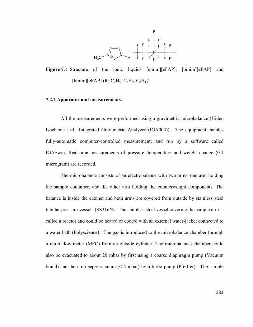
283

Figure 7.1 Structure of the ionic liquids [emim][eFAP], [bmim][eFAP] and

[hmim][eFAP] (R=C2H5, C4H9, C6H13)

7.2.2 Apparatus and measurements.

All the measurements were performed using a gravimetric microbalance (Hiden

Isochema Ltd., Integrated Gravimetric Analyzer (IGA003)). The equipment enables

fully-automatic computer-controlled measurement; and run by a software called

IGASwin. Real-time measurements of pressure, temperature and weight change (0.1

microgram) are recorded.

The microbalance consists of an electrobalance with two arms, one arm holding

the sample container, and the other arm holding the counterweight components. The

balance is inside the cabinet and both arms are covered from outside by stainless steel

tubular pressure-vessels (SS316N). The stainless steel vessel covering the sample arm is

called a reactor and could be heated or cooled with an external water-jacket connected to

a water bath (Polyscience). The gas is introduced to the microbalance chamber through

a multi flow-meter (MFC) from an outside cylinder. The microbalance chamber could

also be evacuated to about 20 mbar by first using a coarse diaphragm pump (Vacuum

brand) and then to deeper vacuum (< 5 mbar) by a turbo pump (Pfeiffer). The sample

284

temperature was measured with a platinum resistance thermocouple (± 0.1 K), and

pressure was measured with a pressure transducer (Druck PDCR 4010, ± 8 mbar).

Sample between 50-80 mg were loaded into the sample container and properly

sealed. The samples were heated to 348.2 K under deep vacuum in the chart mode to

outgas water and other impurities until the weight was stabilized. The temperature was

then reset to the experimental temperature. Once the desired temperature was reached,

CO2 was introduced to the reactor until the first isotherm pressure was reached.

Continuous absorption data was recorded until 99% of the predicted equilibrium weight

was reached. After that, measurement at the next isotherm pressure is continued and

continues until measurement is done at all the pressure points under the isotherm.

An important step in obtaining accurate data from gravimetric method using IGA

is buoyancy correction to the weight as the sample remains immersed in the gas in the

pressure vessel. The gas solubilities in ILs were determined from real-time equilibrium

mass uptake at a given pressure and temperature with appropriate buoyancy correction.

A blank experiment (without any sample) was run for each isotherm and at all pressures

with the same bucket. The real-time weights obtained from these runs were used to

nullify the buoyancy corrections due to all the components of the balance and the bucket

and balance sensitivity.

Density of ionic liquid, required for buoyancy correction due to solvent was

measured using Anton Paar digital density meter DMA 4500 (accuracy ± .00005 g/cm3)

in the temperature range between 283.15 K and 353.15 K with 5 K interval at

atmospheric pressure. It measures liquid density based on the oscillating U-tube

principle. The machine was calibrated with air and water following the instruction

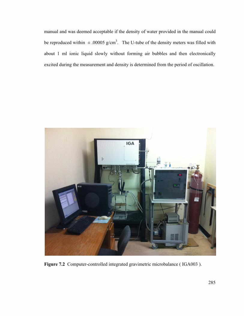
285

manual and was deemed acceptable if the density of water provided in the manual could

be reproduced within ± .00005 g/cm3. The U-tube of the density meters was filled with

about 1 ml ionic liquid slowly without forming air bubbles and then electronically

excited during the measurement and density is determined from the period of oscillation.

Figure 7.2 Computer-controlled integrated gravimetric microbalance ( IGA003 ).

286

7.3 MODELING

CO2-IL system is a complex non-ideal system characterized by the large

differences in shape and size and the presence of ionic interactions. Cubic equations of

state, originally developed for modeling phase equilibrium for non-electrolyte systems,

were recently used successfully for modeling many ionic liquids+CO2 systems. While

not deeply rooted in statistical mechanics, their relatively simple algebraic form capable

of representing two phases and the need for few adjustable parameters have made them

popular choice in design and analysis of many industrial complex VLE process. The

solubility data were correlated with the Peng-Robinson equation of state (equation 7.1)

with two-fluid mixing rule.2

2

(7.1)

Where and are the mixture attractive and co-volume parameters, respectively and

related to the corresponding pure component parameters with van der Waals quadratic

two parameter mixing rules.

(7.2)

(7.3)

where

1

with and 1

(7.4)

287

1

2

with and 1

(7.5)

And the pure component attractive and co-volume parameters and are related to the

critical temperature ( ) , critical pressure ( ) and accentric factor ( ) as

(7.6)

0.45724

(7.7)

0.37464 1.5422 0.26992 (7.8)

0.0778

(7.9)

Critical properties of ionic liquids were estimated using Group-contribution

methods.3 The binary interaction parameters were regressed using the software Phase

Equilibrium 2000 (PE2000)4 developed by Brunner and coworkers that uses a Simplex-

Nelder-Mead algorithm for regression. The average absolute relative deviation (equation

7.10) in the liquid phase mole fraction was minimized at experimental temperature and

pressure.

100% (7.10)

288


The densities of the ionic liquids were measured between 283.15 K and 353.15 K

in 5 K interval and the data reported in Table 7.1. The number of various functional

groups present in the ionic liquids required for computation of critical properties is

tabulated in Table 7.2 and the estimated critical properties of the ionic liquids required

for modeling are presented in Table 7.3. To verify our experimental method, solubility

data of CO2 in a common ionic liquid [bmim][PF6] at 25°C were measured and

compared with those reported by Anthony et al. (2002)5 and Shiflett et al. (2005)6 in

Figure 7.3. The average absolute deviation between the data of Shiflett et al.6 and this

work is 0.001 in mole fraction of CO2.

The solubility data of CO2 in the ionic liquids [emim][eFAP], [bmim][eFAP] and

[hmim][eFAP] were then measured and reported in Tables 7.4, 7.6 and 7.8 in mole-

fraction scale and in Tables 7.5, 7.7 and 7.9 in molality scale (mol CO2/kg IL)

respectively. The solubility data presented in Tables 7.4, 7.6 and 7.8 are also plotted in

Figures 7.4, 7.5, and 7.6 respectively with modeling results.

The measured solubility data of CO2 in [hmim][eFAP] was compared with

literature data in Figure 7.7. At low pressure, good agreement is found with the data of

both Muldoon et al.(2007)7 and Zhang et al. (2008)8; but, at higher pressure, slight

discrepancies appear from the data of Zhang et al. (2008). The measured solubility data

of CO2 in [emim][eFAP] was in good agreement with the high-pressure bubble-point

data of Althuluth et al. (2012)9 (Figure 7.8).

289

Table 7.1 Measured Density of Ionic Liquids

Ionic Liquids

T(K) [bmim][PF6] [emim][eFAP] [bmim][eFAP] [hmim][eFAP]

283.15 1.37892 1.72709 1.64218 1.56636

288.15 1.37464 1.72114 1.63654 1.56059

293.15 1.37037 1.71519 1.63089 1.55553

298.15 1.36611 1.70923 1.62524 1.5501

303.15 1.36185 1.7033 1.61959 1.54467

308.15 1.35775 1.69738 1.61395 1.53927

313.15 1.35365 1.69148 1.60833 1.53387

318.15 1.34954 1.68559 1.60272 1.52848

323.15 1.34544 1.67972 1.59713 1.52311

328.15 1.34135 1.67387 1.59155 1.51775

333.15 1.33727 1.66803 1.58598 1.51241

338.15 1.3332 1.66221 1.58044 1.50708

343.15 1.32914 1.65641 1.57491 1.50176

348.15 1.32509 1.65063 1.56939 1.49647

353.15 1.32107 1.64487 1.56391 1.49119

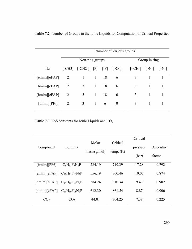
290

Table 7.2 Number of Groups in the Ionic Liquids for Computation of Critical Properties

Number of various groups

Non-ring groups Group in ring

ILs [-CH3] [-CH2-] [P] [-F] [>C<] [=CH-] [>N-] [=N-]

[emim][eFAP] 2 1 1 18 6 3 1 1

[bmim][eFAP] 2 3 1 18 6 3 1 1

[hmim][eFAP] 2 5 1 18 6 3 1 1

[bmim][PF6] 2 3 1 6 0 3 1 1

Table 7.3 EoS constants for Ionic Liquids and CO2.

Component Formula Molar

mass/(g/mol)

Critical

temp. (K)

Critical

pressure

(bar)

Accentric

factor

[bmim][PF6] C8H15F6N2P 284.19 719.39 17.28 0.792

[emim][eFAP] C12H11F18N2P 556.19 760.46 10.05 0.874

[bmim][eFAP] C14H15F18N2P 584.24 810.34 9.43 0.902

[hmim][eFAP] C16H19F18N2P 612.30 861.54 8.87 0.906

CO2 CO2 44.01 304.25 7.38 0.225

291

Figure 7.3 Comparison of solubility of CO2 in [bmim][PF6] with literature data.

0

0.5

1

1.5

2

2.5

0.0 0.1 0.2 0.3 0.4

Tot

al p

ress

ure

, PM

Pa

Mole fraction of CO2 in [bmim][PF6]

Anthony et al. (2002) (Ref. 5)Shiflett et al. (2005) (Ref. 6)This work

292

Table 7.4 Solubility of CO2 in [emim][eFAP] at Different Pressures and Temperatures

in the Mole-Fraction scale

P (MPa) Mole

Fraction P (MPa)

Mole

Fraction P (MPa)

Mole

Fraction

T=283.15K T=298.15K T=323.15K

0.05 0.023 0.05 0.019 0.05 0.012

0.10 0.048 0.10 0.037 0.10 0.024

0.30 0.137 0.30 0.103 0.30 0.065

0.50 0.213 0.50 0.162 0.50 0.112

0.70 0.280 0.70 0.217 0.70 0.150

1.00 0.364 1.00 0.287 1.00 0.203

1.20 0.413 1.20 0.330 1.20 0.236

1.40 0.456 1.40 0.365 1.40 0.267

1.60 0.495 1.60 0.402 1.60 0.294

1.80 0.530 1.80 0.440 1.80 0.321

2.00 0.562 1.99 0.462 2.00 0.345

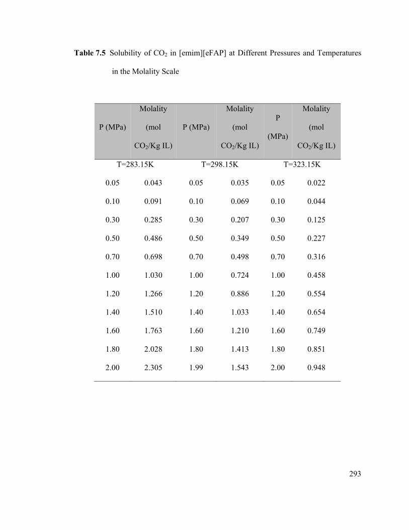
293

Table 7.5 Solubility of CO2 in [emim][eFAP] at Different Pressures and Temperatures

in the Molality Scale

P (MPa)

Molality

(mol

CO2/Kg IL)

P (MPa)

Molality

(mol

CO2/Kg IL)

P

(MPa)

Molality

(mol

CO2/Kg IL)

T=283.15K T=298.15K T=323.15K

0.05 0.043 0.05 0.035 0.05 0.022

0.10 0.091 0.10 0.069 0.10 0.044

0.30 0.285 0.30 0.207 0.30 0.125

0.50 0.486 0.50 0.349 0.50 0.227

0.70 0.698 0.70 0.498 0.70 0.316

1.00 1.030 1.00 0.724 1.00 0.458

1.20 1.266 1.20 0.886 1.20 0.554

1.40 1.510 1.40 1.033 1.40 0.654

1.60 1.763 1.60 1.210 1.60 0.749

1.80 2.028 1.80 1.413 1.80 0.851

2.00 2.305 1.99 1.543 2.00 0.948

294

Table 7.6 Solubility of CO2 in [bmim][eFAP] at Different Pressures and Temperatures

in the Mole-Fraction Scale

P (MPa) Mole

Fraction P (MPa)

Mole

Fraction P (MPa)

Mole

Fraction

T=283.15K T=298.15K T=323.15K

0.05 0.027 0.05 0.021 0.05 0.013

0.10 0.052 0.10 0.040 0.10 0.025

0.30 0.144 0.30 0.109 0.30 0.071

0.50 0.223 0.50 0.176 0.50 0.118

0.70 0.290 0.70 0.229 0.70 0.157

0.90 0.342 0.90 0.274 0.90 0.189

1.00 0.377 1.00 0.301 1.00 0.214

1.20 0.426 1.20 0.345 1.20 0.249

1.40 0.470 1.40 0.384 1.40 0.281

1.60 0.509 1.60 0.419 1.60 0.310

1.80 0.544 1.80 0.452 1.80 0.338

2.00 0.576 2.00 0.481 2.00 0.363

295

Table 7.7 Solubility of CO2 in [bmim][eFAP] at Different Pressures and Temperatures


P (MPa)

Molality

(mol

CO2/Kg

IL)

P (MPa)

Molality

(mol

CO2/Kg

IL)

P (MPa)

Molality

(mol

CO2/Kg

IL)

T=283.15K T=298.15K T=323.15K

0.05 0.047 0.05 0.036 0.05 0.023

0.10 0.094 0.10 0.071 0.10 0.044

0.30 0.288 0.30 0.210 0.30 0.130

0.50 0.490 0.50 0.366 0.50 0.229

0.70 0.701 0.70 0.509 0.70 0.320

0.90 0.891 0.90 0.645 0.90 0.400

1.00 1.036 1.00 0.737 1.00 0.467

1.20 1.271 1.20 0.900 1.20 0.566

1.40 1.518 1.40 1.066 1.40 0.670

1.60 1.774 1.60 1.236 1.60 0.771

1.80 2.041 1.80 1.409 1.80 0.876

2.00 2.325 2.00 1.586 2.00 0.975

296

Table 7.8 Solubility of CO2 in [hmim][eFAP] at Different Pressures and Temperatures

in the Mole Fraction Scale

P (MPa)

Mole

Fraction P (MPa)

Mole

Fraction P (MPa)

Mole

Fraction

T=283.15K T=298.15K T=323.15K

0.05 0.029 0.05 0.023 0.05 0.016

0.10 0.055 0.10 0.044 0.10 0.029

0.30 0.150 0.30 0.115 0.30 0.078

0.50 0.230 0.50 0.185 0.50 0.127

0.70 0.300 0.70 0.239 0.70 0.167

1.00 0.388 1.00 0.314 1.00 0.224

1.20 0.438 1.20 0.358 1.20 0.258

1.40 0.482 1.40 0.397 1.40 0.291

1.60 0.521 1.60 0.433 1.60 0.320

1.80 0.556 1.80 0.465 1.80 0.348

2.00 0.588 2.00 0.494 2.00 0.374

297

Table 7.9 Solubility of CO2 in [hmim][eFAP] at Different Pressures and Temperatures


P (MPa)

Molality

(mol

CO2/Kg

IL)

P (MPa)

Molality

(mol

CO2/Kg

IL)

P (MPa)

Molality

(mol

CO2/Kg

IL)

T=283.15K T=298.15K T=323.15K

0.05 0.048 0.05 0.039 0.05 0.027

0.10 0.095 0.10 0.075 0.10 0.049

0.30 0.288 0.30 0.213 0.30 0.137

0.50 0.488 0.50 0.371 0.50 0.237

0.70 0.699 0.70 0.514 0.70 0.328

1.00 1.035 1.00 0.746 1.00 0.472

1.20 1.272 1.20 0.910 1.20 0.569

1.40 1.519 1.40 1.075 1.40 0.672

1.60 1.775 1.60 1.245 1.60 0.769

1.80 2.042 1.80 1.417 1.80 0.872

2.00 2.329 2.00 1.592 2.00 0.976

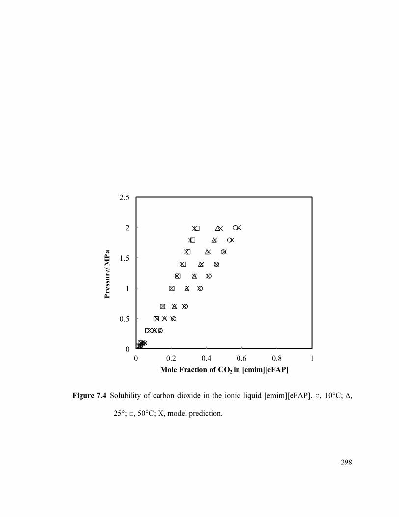
298

Figure 7.4 Solubility of carbon dioxide in the ionic liquid [emim][eFAP]. ○, 10°C; ∆,

25°; □, 50°C; X, model prediction.

0

0.5

1

1.5

2

2.5

0 0.2 0.4 0.6 0.8 1

Pre

ssu

re/ M

Pa

Mole Fraction of CO2 in [emim][eFAP]

299

Figure 7.5 Solubility of carbon dioxide in the ionic liquid [bmim][eFAP]. ○, 10°C; ∆,

25°C; □, 50°C, X, model prediction.

0

0.5

1

1.5

2

2.5

0 0.2 0.4 0.6 0.8 1

Pre

ssu

re/ M

Pa

Mole fraction of CO2 in [bmim][eFAP]

300

Figure 7.6 Solubility of carbon dioxide in the ionic liquid [hmim][eFAP]: ○, 10°C; ∆,

25°C; □, 50°C, X, model prediction.

0

0.5

1

1.5

2

2.5

0 0.2 0.4 0.6 0.8 1

Pre

ssu

re/ M

Pa

Mole fraction of CO2 in [hmim][eFAP]

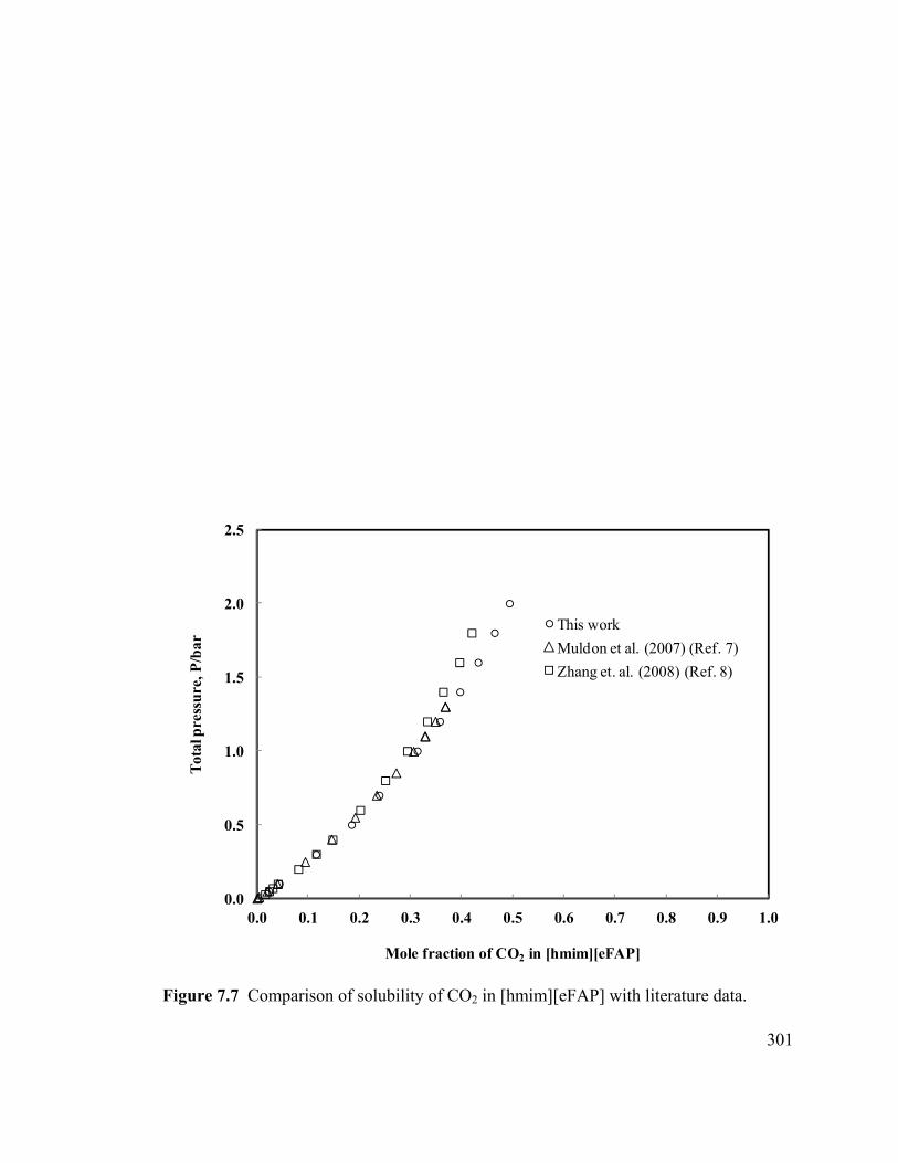
301

Figure 7.7 Comparison of solubility of CO2 in [hmim][eFAP] with literature data.

0.0

0.5

1.0

1.5

2.0

2.5

0.0 0.1 0.2 0.3 0.4 0.5 0.6 0.7 0.8 0.9 1.0

Tot

al p

ress

ure

, P/b

ar

Mole fraction of CO2 in [hmim][eFAP]

This work

Muldon et al. (2007) (Ref. 7)

Zhang et. al. (2008) (Ref. 8)

302

Figure 7.8 Comparison of solubility of CO2 in [emim][eFAP] with literature data.

0

0.5

1

1.5

2

2.5

0.0 0.1 0.2 0.3 0.4 0.5 0.6 0.7 0.8 0.9 1.0

Tot

al p

ress

ure

, P/b

ar

Mole Fraction of CO2 in [hmim][eFAP]

Althuluth et al. (2012) (Ref. 9), 284 K

This work, 283K

Althuluth et al. (2012) (Ref. 9), 324 K

This work, 323K

303

The temperature-dependent binary interaction parameters for Peng-Robinson EoS

and the corresponding absolute average deviation calculated using the objective function

(equation 7.10) is given in Table 7.10. The solubility data was correlated well with one

binary interaction parameter within the pressure and temperature range of the

experimental data used in correlation. Solubility increases quickly with pressure. The

effect of temperature is less at low pressure but gets more pronounced as the pressure

increases.

For many ionic liquids, experimental measurements at high pressure showed that

after a certain concentration of CO2 is dissolved in the liquid phase, very high pressure is

required to further dissolve CO2 in the ionic liquid (Aki et al., 2004).10 This behavior is

explained by free-volume theory that solubility of CO2 increases with pressure fast at

low pressure when CO2 starts occupying the free-spaces in the ionic liquid structure, but

once the free-space is filled, it requires very high-pressure to increase the solubility even

nominally resulting in an infinite P-x slope (diverging bubble point and dew point

pressure curve) (Blanchard. et al., 2001).11 The present EoS with one optimized binary

interaction parameter did not reproduce this behavior, it predicts a mixture critical point

where bubble point and dew point curves meet at high CO2 mole fraction (Figure 7.9).

Similar modeling results was also found by Ren et al. (2010)12 for {carbon dioxide (CO2)

+ n-hexyl-imidazolium bis[(trifluoromethyl)sulfonyl]amide} system who correlated

high-pressure data by the PR EoS with two binary interaction parameters. Re-optimizing

the binary parameters using one high-pressure data point from the measurement of

Althuluth et al. (2012)9 for the ionic liquids [emim][eFAP] reveals the typical high-

pressure phase behavior that the pressure-composition curve diverges after a certain

304

amount of CO2 dissolution (Figure 7.9). In this case, two binary interaction parameters

were required (kij=0.0832, lij=0.0392) to correlate the solubility data. Moreover,

prediction of high-pressure phase behavior using these parameters (without re-

optimizing) at 25°C, also reveals a VLLE phase at high pressure (Figure 7.10), and such

phase behavior is also predicted by cubic EoS modeling for other ionic liquids such as

[bmim][PF6] (Shiflett et al.,2005), [bmim][acetate] (Shiflett et al., 2008)13 and

[hmim][Tf2N] (Ren et al., 2010)12 below the critical temperature of CO2. However,

such extrapolation is cautioned in absence of experimental evidence due to the inherent

weaknesses of cubic equation of state for the present system due to the poor theoretical

basis of cubic EoS for polar and associating fluids in general, and relevant to the present

systems, there is no explicit ionic interaction term in the EoS (Reissi et al., 2010).14

305

Table 7.10 Estimated Binary Interaction Parameters and Modeling Results

Ils+CO2 T/K

Number

of data

points

Binary interaction

parameters

kij lij AARD%

[emim][eFAP] 283.15 11 - 0.021 1.92

298.15 13 - 0.020 1.24

323.15 11 - 0.014 1.52

[bmim][Tf2N] 283.15 12 - 0.023 1.16

298.15 12 - 0.022 0.75

323.15 12 - 0.018 0.71

[hmim][Tf2N] 283.15 11 - 0.023 1.33

298.15 11 - 0.024 0.61

323.15 11 - 0.019 1.82

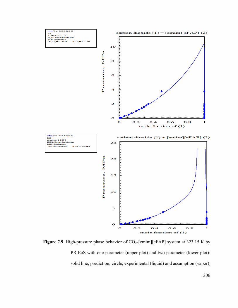
306


PR EoS with one-parameter (upper plot) and two-parameter (lower plot):

solid line, prediction; circle, experimental (liquid) and assumption (vapor).

307


PR EoS with one-parameter (upper plot) and two-parameter (lower plot):

solid line, prediction; circle, experimental (liquid) and assumption (vapor).

308

The mole-fraction based Henry’s law constant is defined in equation 7.11. At

equilibrium, the fugacities of the solute gas in both phases are equal (equation 7.12).

Moreover, assuming the gas phase is essentially free of ionic liquid, the fugacity of vapor

phase is assumed to be equal to that of pure carbon dioxide at the same temperature and

pressure which is computed using the Peng-Robinson equation of state. Thus Henry’s

law constant is computed from the linear slope of fugacity versus mole-fraction curve at

low pressure (equation 7.14).

lim

(7.11)

, , , , (7.12)

, , , (7.13)

lim lim

,

(7.14)

The calculated Henry’s law constants are presented in Table 7.11 and in Figure

7.11. Henry’s law constants decrease with both increase in alkyl chain length and

increase in temperature. The Henry’s law constant of [emim][eFAP] at 283.15 is 2.14

MPa, comparable with 2.24 MPa reported by Althuluth et al. (2012)9 and Henry’s law

constant of [hmim][eFAP] at 25°C are comparable with those of 2.52 MPa by Muldoon

et al. (2007)7 and 2.37 MPa by Zhang et al. (2008)8. Henry’s law constants at 25°C in

[emim][eFAP], [bmim][eFAP], and in [hmim][eFAP] are slightly higher than the

corresponding COSMO-RS prediction of 2.1, 2.0 and 1.9 MPa presented in the previous

chapter. The effect of temperature on gas solubility is expressed in terms of enthalpy and

entropy of solvation in Table 7.12. Both values become less negative with increase in

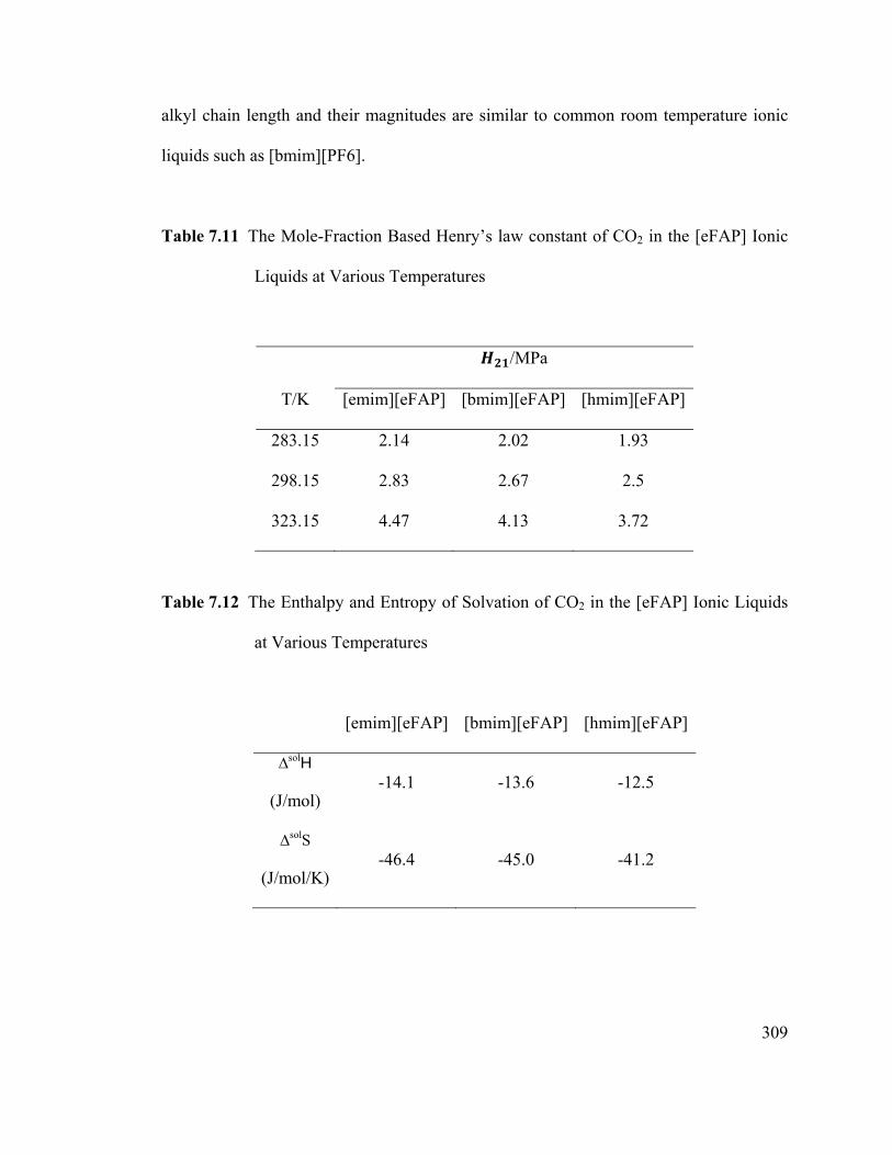
309

alkyl chain length and their magnitudes are similar to common room temperature ionic

liquids such as [bmim][PF6].

Table 7.11 The Mole-Fraction Based Henry’s law constant of CO2 in the [eFAP] Ionic

Liquids at Various Temperatures

/MPa

T/K [emim][eFAP] [bmim][eFAP] [hmim][eFAP]

283.15 2.14 2.02 1.93

298.15 2.83 2.67 2.5

323.15 4.47 4.13 3.72

Table 7.12 The Enthalpy and Entropy of Solvation of CO2 in the [eFAP] Ionic Liquids

at Various Temperatures

[emim][eFAP] [bmim][eFAP] [hmim][eFAP]

∆solH

(J/mol) -14.1 -13.6 -12.5

∆solS

(J/mol/K) -46.4 -45.0 -41.2

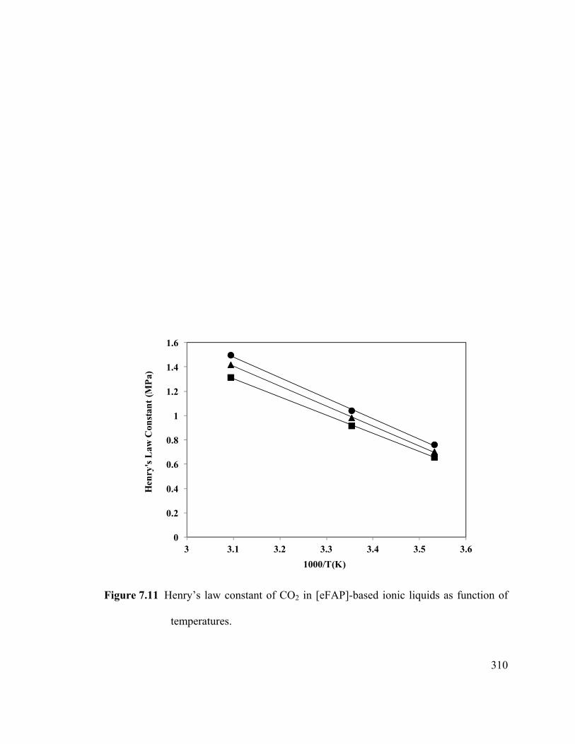
310

Figure 7.11 Henry’s law constant of CO2 in [eFAP]-based ionic liquids as function of

temperatures.

0

0.2

0.4

0.6

0.8

1

1.2

1.4

1.6

3 3.1 3.2 3.3 3.4 3.5 3.6

Hen

ry's

Law

Con

stan

t (M

Pa)

1000/T(K)

311

7.5 CONCLUSIONS

The solubility of CO2 in the ionic liquids based on [eFAP] is presented at

temperatures (283.15, 298.15 and 323.15) K and at pressures (0.5 to 2) MPa. The

solubility data were in good agreement with literature data. The solubility data were

correlated with Peng-Robinson equation of state. Henry's law constants of CO2 in these

ionic liquid are derived and was in good agreement with literature data and COSMO-RS

prediction. The measured Henry’s law constants at 25°C in [emim][eFAP],

[bmim][eFAP], and in [hmim][eFAP] are 2.83, 2.67 and 2.5 MPa.

312

7.6 REFERENCES

1. Ignat’ev, N. V.; Welz-Biermann, U.; Kucheryna, A.; Bissky, G.; Willner, H. New

Ionic Liquids with Tris(perfluoroalkyl)trifluorophosphate (FAP) Anions. J.

Fluorine Chem. 2005, 126, 1150.

2. Peng, D. Y.; Robinson, D. B.A New Two-constant Equation of State. Ind. Eng.

Chem. Res. 1976, 15, 59.

3. Valderrama, J. O.; Rojas, R. E. Critical Properties of Ionic Liquids. Revisited.

Ind. Eng. Chem. Res. 2009, 48, 6890.

4. Pfohl, O.; Petkov, S.; Brunner, G. PE 2000 – A Powerful Tool to Correlate

Phase Equilibria. Herbert Utz Verlag, München, 2000.

5. Anthony, J. L.; Maginn, E. J.; Brennecke, J. F. Solubilities and Thermodynamic

Properties of Gases in the Ionic Liquid 1-n-Butyl-3-methylimidazolium

hexafluorophosphate. J. Phys. Chem. B 2002, 106, 7315.

6. Shiflett, M. B.; Yokoseki, A. Solubilities and Diffusivities of Carbon Dioxide in

Ionic Liquids: [bmim][PF6] and [bmim][BF4]. Ind. Eng. Chem.

Res. 2005, 44, 4453.

7. Muldoon, M. J.; Aki, S. N. V. K.; Anderson, J. L.; Dixon, J. K.; Brennecke, J. F.

Improving Carbon Dioxide Solubility in Ionic Liquids. J. Phys. Chem. B 2007,

111, 9001.

8. Zhang, X. C.; Liu, Z. P.; Wang, W. C. Screening of Ionic Liquids to Capture CO2

by COSMO-RS and Experiments. AIChE J. 2008, 54, 2717.

313

9. Althuluth, M.; Mota-Martinez, M.; Kroon, M. C.; Peters, C. J. Solubility of

Carbon Dioxide in the Ionic Liquid 1-Ethyl-3-methylimidazolium

tris(pentafluoroethyl)trifluorophosphate. J. Chem. Eng. Data 2012, 57 (12),

3422.

10. Aki, S. N. V. K.; Mellein, B. R.; Saurer, E. M.; Brennecke, J. F. High-Pressure

Phase Behavior of Carbon Dioxide with Imidazolium-Based Ionic Liquids. J.

Phys. Chem. B 2004, 108, 20355.

11. Blanchard L. A.; Gu Z. Y.; Brennecke J. F. High-pressure Phase Behavior of

Ionic Liquid/CO2 Systems. J Phys Chem. B. 2001, 105, 2437.

12. Ren, W.; Sensenich1, B.; Scurto, A. M. High-pressure Phase Equilibria of

{Carbon Dioxide (CO2) + n-Alkyl-Imidazolium

Bis(trifluoromethylsulfonyl)amide} Ionic Liquids. J. Chem. Thermodyn. 2010,

42, 305.

13. Shiflett, M. B.; Kasprzak, D. J.; Junk, C. P.; Yokozeki, A. Phase Behavior of

{Carbon Dioxide + [bmim][Ac]} Mixtures. J. Chem. Thermodyn. 2008, 40, 25.

14. Raeissi, S.; Florusse, L.; Peters, C. J. Scott–Van Konynenburg Phase Diagram of

Carbon Dioxide + Alkylimidazolium-Based Ionic Liquids. J. of Supercritical

Fluids 2010, 55, 825.

314

Chapter 8: Density, Viscosity and Excess Enthalpy of { 1-Butyl-3-Methyl Imidazolium

Acetate+Water} System _______________________________________________________________________

8.1 INTRODUCION

Aqueous mixture of the ionic liquid 1-butyl-3-methyl imidazolium acetate

([bmim][Ac]) is a patented solvent for CO2 separation.1 The {CO2+([bmim][Ac]}

system has spurred much interest in recent years due to high solubility of CO2 in

[bmim][Ac] and has been subject to many computational and experimental

investigations. The solubility of CO2 in 1-butyl-3-methylimidazolium acetate as a

function of temperature and pressure was measured by various researchers.2-5 The

distinct phase behavior of CO2 with [bmim][Ac] was attributed to chemical absorption

rather than physical absorption by spectroscopic and computational study.6-8 An

economic evaluation of CO2 capture using [bmim][Ac] was carried out using process

simulation.9 Effect of water on solubility of CO2 and physical properties of [bmim][Ac]

was recently studied.4 Addition of water decreases solubility of CO2, but dramatically

reduces the viscosity and thus expected to reduce overall cost of capture.4

Knowledge of various thermo physical properties is required for engineering

design and subsequent operations. We have measured the density, viscosity, and excess

enthalpies of {[bmim][Ac]+water} at various temperatures over the whole composition

315

range. The temperature and composition dependence of these properties is analyzed and

correlated. Excess enthalpy of {water+[bmim][Ac]} system was compared with those of

{amine+[bmim][Ac]} system.

8.2 EXPERIMENTAL

1-butyl-3-methyl-imidazolium acetate (CAS No. 284049-75-8) was obtained

from Sigma-Aldrich (assay ≥95% mas percent) and was used without further

purification. The water content of the ionic liquid changed during experiments and was

measured on average to be 6000 ppm (Karl-Fisher coulometric titration). The amines

monoethanolamine (≥98% mass percent) (CAS 141-43-5), diethanolamine, (≥98% mass

percent) (CAS 111-42-2), triethanolamine (≥99% mass percent) (CAS 102-71-6) , 2-

amino-2-methyl-1-propanol (≥99% mass percent) (CAS 124-68-5), N-methyl

diethanolamine (≥99% mass percent) (CAS 105-59-9) were obtained from Sigma Adrich

and was used without further purification. The solutions were prepared by mass on an

analytical balance (model Ap 205D, Ohaus, Florham Park, NJ) with ± 0.01 mg accuracy.

Densities of the binary mixtures were measured with an Anton Paar DMA-4500

density meter as described in chapter 7. Density was adjusted with air and bidistilled

degassed waster for the full temperature range as is recommend by the manufacturer

(uncertainties are about ± 5E-5 g.cm3). Kinematic viscosities (ν) were determined with

a number of Cannon-Ubbelohde viscometers (Cole-Parmer) to cover the whole

composition and temperature range (25°C to 70°C). The temperature was controlled by

means of a digital controller (± 0.004°C) in a well-stirred bath within ±0.01°C as

316

measured by a Cole-Parmer resistance thermometer (model H-01158-65, Anjou, Québec,

Canada). The efflux time was averaged over repeated measurements with a handhold

digital stopwatch capable of measuring time within ±0.01s. The value of the dynamic

viscosity (η) was obtained by multiplying the measured kinematic viscosities by the

density (ρ). Excess enthalpy of mixing was measured using a C80 Calvet type

calorimeter (Setaram Instrumentation) following procedure described in details in earlier

work.10


The densities of {[bmim][Ac]+water} system are reported in Table 1 and the

densities of pure [bmim][Ac] at various temperatures are compared with literature values

in Figure 8.1. The experimentally measured densities of the aqueous [bmim][Ac]

solutions at (283.15 to 353.15) °C throughout the whole concentration range are

presented in Figure 8.2. Density of the binary mixture slightly increases upon addition

of water and a maximum is seen in the mixture density at nearly 75 mol% water at all

temperature. After the maximum, the density to decrease sharply upon further addition of

water. This behavior is observed at all temperatures but the maximum get less

pronounced with increase in temperature.

The excess molar volume ) was calculated from the raw data by the following

equation and shown in Figures 8.3. All the excess properties display negative deviation,

(8.1)

317

where ( ) is the molar volume of the liquid mixture, and ( ) and ( ) are the mole

fraction and molar volume of the component ( ) respectively. In terms of density, the

excess molar volume is expressed as,

1 1 (8.2)

where is the density of the liquid mixture, and and are the molecular weight and

density of the component . The values of as a function of addition of water are

shown in Figure 8.3. All excess volumes are negative, that is the actual mixture volume

is less than the linear mole-fraction average of the molar volumes of the pure

components. This indicates stronger attractive interaction between water and [bmim][Ac]

to form a more closely packed liquid structure in the binary system than the liquid

structures of each pure component. The degree of close packing kept increasing (

became more negative) with increase in water content and reached a pronounced

minimum at around 70 mol% water at all temperature. After further addition of water,

the excess volumes started to be less native than the minimum. The temperature-

dependence of ( ) is very weak up to 40 mol% water in the mixture and greatly

influence the degree of volume contraction roughly between 70 mol% water and 90

mol% water.

The excess molar volumes were fitted to the Redlich-Kister equation,

(8.3)

318

where and are the mole fraction of water and ionic liquids respectively and

are the temperature-dependent adjustable parameters that were obtained by minimizing

the standard deviation ( )

, , / (8.4)

where is the number of experimental points and is the number of parameters used in

the regression. The regressed values of the coefficients and along with standard

deviation are given in Table 8.2.

To show the effect of temperature on density, the experimental data were also

correlated as a function of temperature for various compositions using the following

polynomial equation. The regressed parameters are presented in Table 8.3 with standard

deviations. Density decreases with increase in temperature at all compositions (Figure

8.3).

(8.5)

The volume expansivity of pure [bmim][Ac] can be calculated by the following equation

(-0.00057K-1 at 298.15 K and -0.00058K-1 at 313.15 K).

1 (8.6)

319

Table 8.1 Density of {[bmim][Ac]+water}System at (283.15 to 353.15) K

Figure 8.1 Comparison of density of [bmim][Ac] with literature data.4,11-14

Mole Fraction of [bmim][Ac]

283.15 K 293.15 K 298.15 K 303.15 K 313.15 K 323.15 K 333.15 K 343.15 K 353.15 K

0.0000 0.99970 0.99820 0.99704 0.99565 0.99221 0.98803 0.98319 0.97776 0.971790.0533 1.04435 1.03874 1.03583 1.03285 1.02672 1.02031 1.01367 1.00678 0.999970.1003 1.06247 1.05580 1.05241 1.04900 1.04211 1.03508 1.02791 1.02064 1.013200.2008 1.07346 1.06686 1.06352 1.06018 1.05341 1.04655 1.03962 1.03260 1.025500.2997 1.07406 1.06777 1.06458 1.06138 1.05493 1.04841 1.04182 1.03517 1.028460.4004 1.07233 1.06625 1.06316 1.06007 1.05382 1.04753 1.04119 1.03480 1.028370.4983 1.06979 1.06372 1.06072 1.05769 1.05161 1.04548 1.03933 1.03315 1.026940.5968 1.06720 1.06109 1.05813 1.05516 1.04916 1.04314 1.03710 1.03106 1.025000.6942 1.06508 1.05896 1.05590 1.05296 1.04702 1.04105 1.03507 1.02910 1.023130.7997 1.06315 1.05704 1.05399 1.05094 1.04504 1.03910 1.03316 1.02724 1.021340.9070 1.06154 1.05534 1.05228 1.04921 1.04325 1.03731 1.03138 1.02547 1.019581.0000 1.06110 1.05472 1.05165 1.04858 1.04259 1.03664 1.03070 1.02480 1.01889

T/K

1.01

1.02

1.03

1.04

1.05

1.06

1.07

1.08

280 300 320 340 360 380

Den

sity

of p

ure

[bm

im][

Ac]

(g/c

m3 )

T/K

Pinkert et al. (2011)

Tariq et al. (2009)

Bogolitsyn et al.(2009)

Almeida et al. (2012)

Stevanovic et al. (2012)

This work

320

Figure 8.2 Densities of binary mixture of water (1) with [bmim][Ac] (2) as a function of

ionic liquid mole fraction (upper plot) and water mole fraction (lower plot)

at various temperatures : ▲, 293.15 K; ●, 298.15 K; □, 303.15 K; ∆, 313.15

K; ○, 323.15 K; ◊, 333.15 K; +,343.15 K; x, 353.15 K; ..., Redlick-Kister

prediction.

0.96

0.98

1

1.02

1.04

1.06

1.08

0 0.2 0.4 0.6 0.8 1

Den

sity

of

aqu

eou

s [b

mim

][A

c](g

/cm

3 )

Mole fraction of water

321

Figure 8.3 Excess molar volumes of binary mixture of water (1) with [bmim][Ac] (2) as

a function of ionic liquid mole fraction at various temperature : ▲, 293.15

K; ●, 298.15 K; □, 303.15 K; ∆, 313.15 K; ○, 323.15 K; ◊, 333.15 K;

+,343.15 K; x, 353.15 K. ..., Redlick-Kister prediction.

-1.6

-1.35

-1.1

-0.85

-0.6

-0.35

-0.1

0 0.1 0.2 0.3 0.4 0.5 0.6 0.7 0.8 0.9 1

Exc

ess

mol

ar v

olu

me

(cm

3 /m

ol)


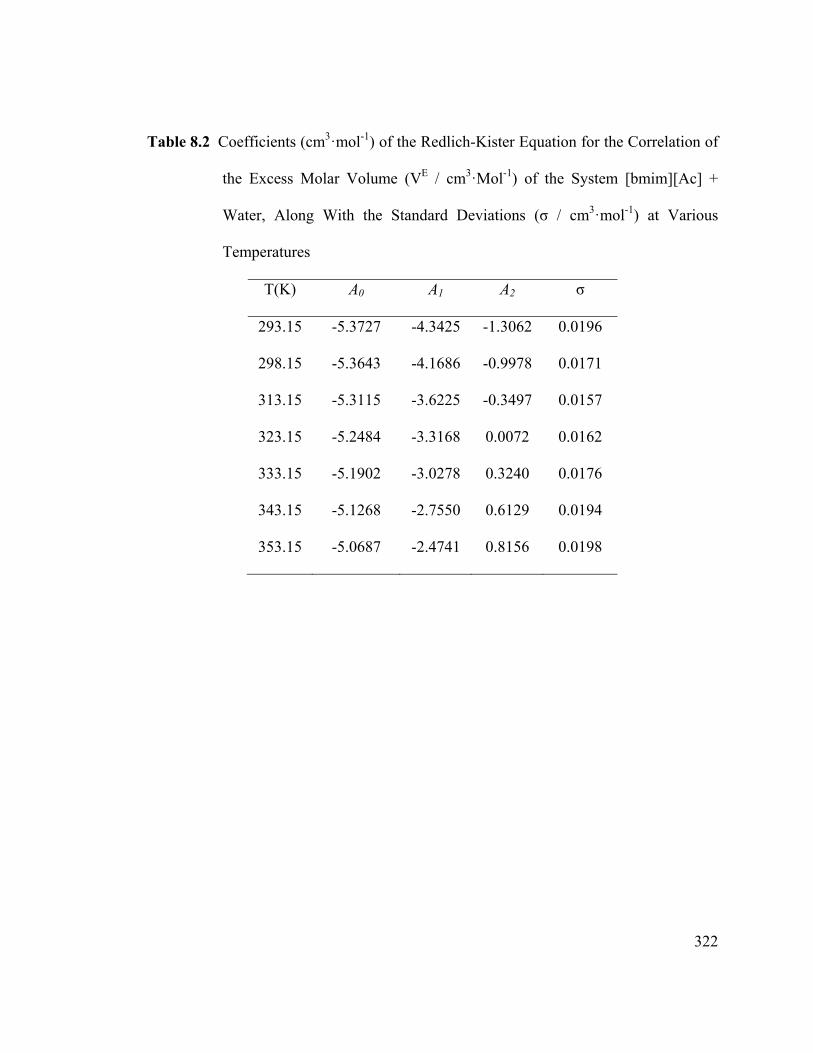
322

Table 8.2 Coefficients (cm3·mol-1) of the Redlich-Kister Equation for the Correlation of

the Excess Molar Volume (VE / cm3·Mol-1) of the System [bmim][Ac] +

Water, Along With the Standard Deviations (σ / cm3·mol-1) at Various

Temperatures

T(K) A0 A1 A2 σ

293.15 -5.3727 -4.3425 -1.3062 0.0196

298.15 -5.3643 -4.1686 -0.9978 0.0171

313.15 -5.3115 -3.6225 -0.3497 0.0157

323.15 -5.2484 -3.3168 0.0072 0.0162

333.15 -5.1902 -3.0278 0.3240 0.0176

343.15 -5.1268 -2.7550 0.6129 0.0194

353.15 -5.0687 -2.4741 0.8156 0.0198

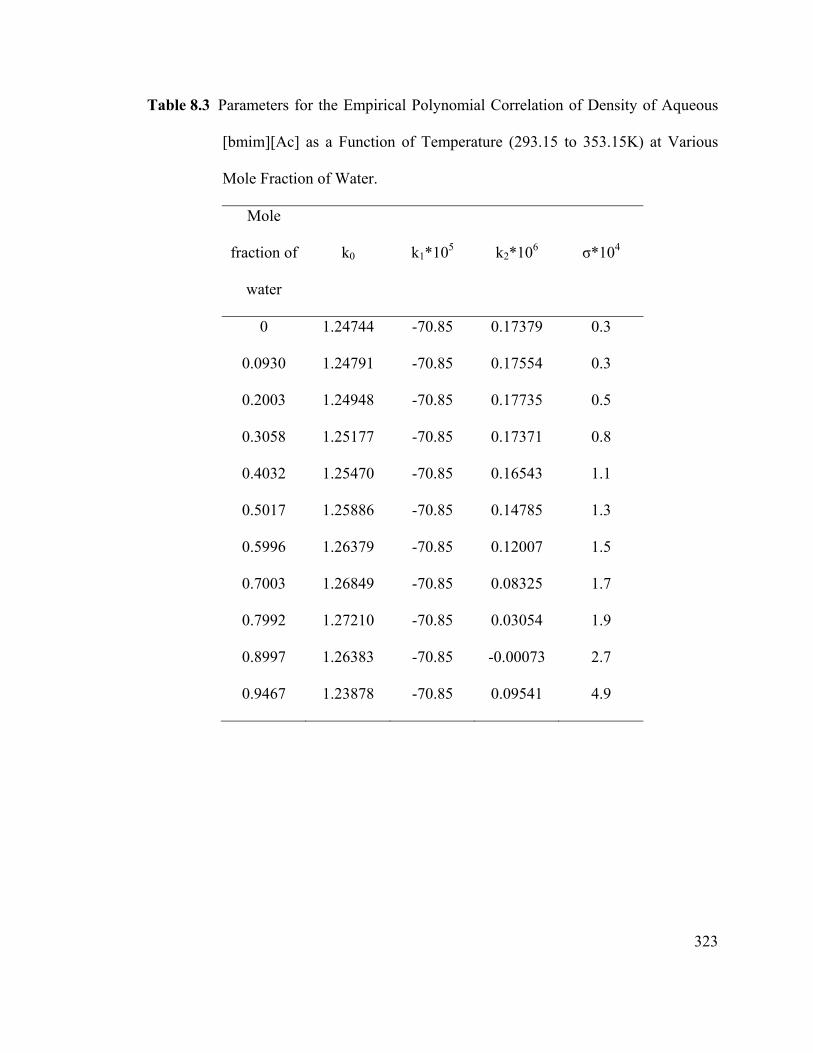
323

Table 8.3 Parameters for the Empirical Polynomial Correlation of Density of Aqueous

[bmim][Ac] as a Function of Temperature (293.15 to 353.15K) at Various

Mole Fraction of Water.

Mole

fraction of

water

k0 k1*105 k2*106 σ*104

0 1.24744 -70.85 0.17379 0.3

0.0930 1.24791 -70.85 0.17554 0.3

0.2003 1.24948 -70.85 0.17735 0.5

0.3058 1.25177 -70.85 0.17371 0.8

0.4032 1.25470 -70.85 0.16543 1.1

0.5017 1.25886 -70.85 0.14785 1.3

0.5996 1.26379 -70.85 0.12007 1.5

0.7003 1.26849 -70.85 0.08325 1.7

0.7992 1.27210 -70.85 0.03054 1.9

0.8997 1.26383 -70.85 -0.00073 2.7

0.9467 1.23878 -70.85 0.09541 4.9

324

Figure 8.4 Effect of temperature on density of binary mixture of water + [bmim][Ac] at

various approximated percent mole fraction of water: ▲, 0%; □, 9%;

+,31%; ○, 50%; ◊, 70%; ∆, 95%; ●, 100%;..., polynomial prediction.

0.96

0.98

1

1.02

1.04

1.06

1.08

290 300 310 320 330 340 350 360

Den

sity

(g/c

m3 )

Temperatrue (K)

325

The experimental data of the viscosities for the {[bmim][Ac]+water} system are

reported in Table 8.4 and the viscosity of pure [bmim][Ac] as a function of temepratrue

is compared with literature data in Figure 8.5. The experimental data of the viscosity for

the binary mixture at different temperatures for the full composition range is presented in

Figure 8.5 as a function of temperature and mole fraction of water. The viscosity values

of pure ionic liquid is high, but decreases quickly with addition of water. This

considerable decrease in viscosity might compensate for the diminished ability of the IL

to dissolve more CO2 in presence of water and at higher temperature. The viscosity

deviation,

∆ (8.7)

were fitted to the Redlich-Kister equation,

∆ (8.8)



the standard deviation ( ) . Viscosity deviations from an ideal mixture viscosity are

negative at all composition. At 298.15K, the viscosity deviation becomes more negative

with addition of water, reaches a minimum at around 50 mole% water, and then becomes

less negative. With increase in temperature, the observed viscosity approaches more

towards the ideal mixture viscosity and at 70°C, the mixture viscosity is only slightly

deviated from an ideal mixture viscosity.

The commonly used two-parameter Arrhenius-type equation was tested to

correlate the temperature-dependence of the observed viscosity data

326

ln ln

(8.9)

where, ∞, is the viscosity at infinite temperature, is the universal gas constant (8.314

J.mol-1.K-1), is the activation energy to flow and is temperature. The parameters

were obtained from a linear plot and presented in Table 8.5. The activation energy to

flow for pure [bmim][Ac] was about 51.4 kJ/mol.

The following Vogel-Fulcher-Tammann (VFT) equation

(8.10)

where, , and 0 are fitting parameters and is temperature, widely used to correlate

liquid viscosity data, was more suitable to correlate the experimental viscosity data. The

parameters are presented in Table 8.6. The value of is 188.9 K, comparable to the

glass-transition temperature of the [bmim][Ac] (203.5K). Viscosity decreases

dramatically with rise in temperature at all concentration (Figure 8.8).17

327

Table 8.4 Viscosity of {[bmim][Ac]+water}System at (298.15 to 343.15) K

Figure 8.5 Comparison of viscosity data of pure [bmim][Ac] with literature data.

Experimental data taken from Ref. 11, 14-16.

Mole Fraction of

[bmim][Ac]298.15 303.15 313.15 323.15 333.15 343.15

0.0533 3.7 3.2 2.4 1.8 1.5 1.20.1003 7.9 6.4 4.6 3.4 2.6 2.10.2008 22.9 18.0 11.9 8.3 6.1 4.60.2997 44.7 34.7 22.0 14.8 10.5 7.70.4004 76.3 58.0 35.4 23.2 16.0 11.50.4983 115.5 86.4 51.4 32.7 22.0 15.60.5968 163.8 120.3 69.4 43.1 28.4 19.80.6942 216.1 155.9 87.5 53.2 34.6 23.70.7997 281.9 200.0 109.1 64.8 41.3 27.80.9070 357.2 249.4 132.0 76.7 48.0 31.91.0000 433.7 297.6 154.0 87.5 54.0 35.3

T/K

0

50

100

150

200

250

300

350

300 320 340 360 380

Vis

cosi

ty(m

Pa.

s)

Temperature/K

Crosthwaite et al. (2005)

Pinket et al. (2012)

Xu et al. (2012)

Almeida et al. (2012)

This work

328

Figure 8.6 Viscosity of binary mixture of water (1) with [bmim][Ac] (2) as a function

of water mole fraction at various temperature : ●, 298.15 K; □, 303.15 K; ∆,

313.15 K; ○, 323.15 K; ◊, 333.15 K; +,343.15 K. ..., Redlick-Kister

prediction.

0

50

100

150

200

250

300

350

400

450

0 0.2 0.4 0.6 0.8 1

Vis

cosi

ty (m

Pa.

s)


329

Figure 8.7 Viscosity deviations of binary mixture of water (1) with [bmim][Ac] (2) as a

function of ionic liquid mole fraction at various temperature : ●, 298.15 K;

□, 303.15 K; ∆, 313.15 K; ○, 323.15 K; ◊, 333.15 K; +,343.15 K. ...,

Redlick-Kister correlation.

-110

-100

-90

-80

-70

-60

-50

-40

-30

-20

-10

00 0.2 0.4 0.6 0.8 1

Vis

cosi

ty d

evia

tion

(m

Pa.

s)


330


Viscosity Deviation (∆η / mPa·s) of the System [bmim][Ac]+Water, and the

Standard Deviations (σ / mPa·s).

T(K) B0 B1 B2 B3 σ

298.15 -402.3368 -20.2604 -16.5342 55.6913 0.42

313.15 -248.4730 -35.7401 -10.3502 34.6251 0.30

323.15 -102.6328 -36.7245 -9.4603 23.0090 0.17

333.15 -44.6907 -23.7759 -6.5823 6.6493 0.21

343.15 -20.4567 -19.8377 -5.6889 8.7746 0.06

353.15 -8.8674 -14.1451 -3.4183 4.3190 0.06

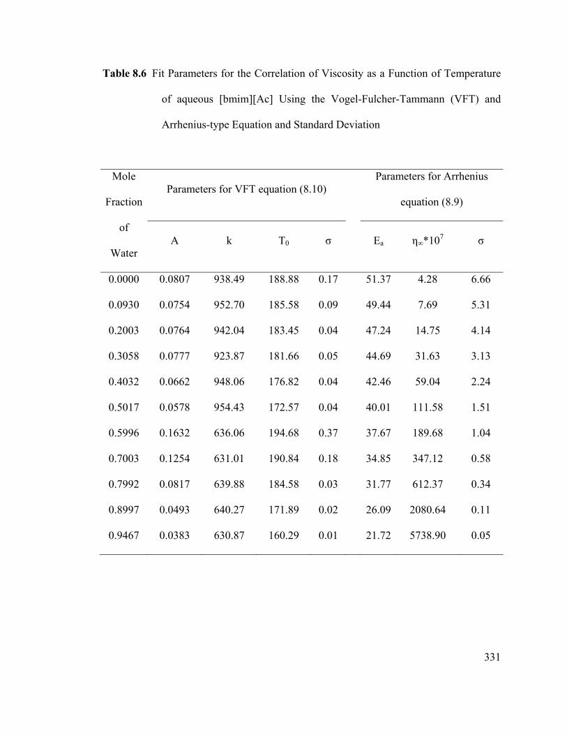
331

Table 8.6 Fit Parameters for the Correlation of Viscosity as a Function of Temperature

of aqueous [bmim][Ac] Using the Vogel-Fulcher-Tammann (VFT) and

Arrhenius-type Equation and Standard Deviation

Mole

Fraction

of

Water

Parameters for VFT equation (8.10)

Parameters for Arrhenius

equation (8.9)

A k T0 σ Ea η∞*107 σ

0.0000 0.0807 938.49 188.88 0.17

51.37 4.28 6.66

0.0930 0.0754 952.70 185.58 0.09

49.44 7.69 5.31

0.2003 0.0764 942.04 183.45 0.04

47.24 14.75 4.14

0.3058 0.0777 923.87 181.66 0.05

44.69 31.63 3.13

0.4032 0.0662 948.06 176.82 0.04

42.46 59.04 2.24

0.5017 0.0578 954.43 172.57 0.04

40.01 111.58 1.51

0.5996 0.1632 636.06 194.68 0.37

37.67 189.68 1.04

0.7003 0.1254 631.01 190.84 0.18

34.85 347.12 0.58

0.7992 0.0817 639.88 184.58 0.03

31.77 612.37 0.34

0.8997 0.0493 640.27 171.89 0.02

26.09 2080.64 0.11

0.9467 0.0383 630.87 160.29 0.01 21.72 5738.90 0.05

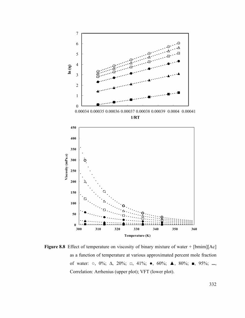
332

Figure 8.8 Effect of temperature on viscosity of binary mixture of water + [bmim][Ac]

as a function of temperature at various approximated percent mole fraction

of water: ○, 0%; ∆, 20%; □, 41%; ●, 60%; ▲, 80%; ■, 95%; ...,

Correlation: Arrhenius (upper plot); VFT (lower plot).

0

1

2

3

4

5

6

7

0.00034 0.00035 0.00036 0.00037 0.00038 0.00039 0.0004 0.00041

ln (η

)

1/RT

0

50

100

150

200

250

300

350

400

450

300 310 320 330 340 350 360

Vis

cosi

ty (m

Pa.

s)

Temperature (K)

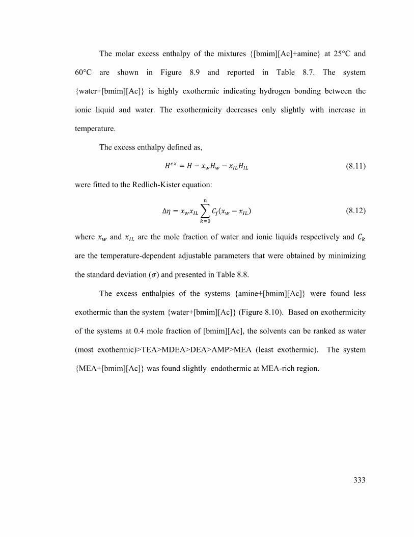
333

The molar excess enthalpy of the mixtures {[bmim][Ac]+amine} at 25°C and

60°C are shown in Figure 8.9 and reported in Table 8.7. The system

{water+[bmim][Ac]} is highly exothermic indicating hydrogen bonding between the

ionic liquid and water. The exothermicity decreases only slightly with increase in

temperature.

The excess enthalpy defined as,

(8.11)

were fitted to the Redlich-Kister equation:

∆ (8.12)



the standard deviation ( ) and presented in Table 8.8.

The excess enthalpies of the systems {amine+[bmim][Ac]} were found less

exothermic than the system {water+[bmim][Ac]} (Figure 8.10). Based on exothermicity

of the systems at 0.4 mole fraction of [bmim][Ac], the solvents can be ranked as water

(most exothermic)>TEA>MDEA>DEA>AMP>MEA (least exothermic). The system

{MEA+[bmim][Ac]} was found slightly endothermic at MEA-rich region.

334

Table 8.7 Viscosity of {[bmim][Ac]+water}System at (298.15 to 343.15) K

Mole

Fraction of

[bmim][Ac]

Excess

Enthalpy

(J/mol) at

25°C

Mole

Fraction of

[bmim][Ac]

Excess

Enthalpy

(J/mol) at 60°C

0.0294 -1259 0.0301 -1093

0.0496 -2008 0.0505 -1445

0.1008 -3536 0.1034 -3284

0.2022 -4943 0.2023 -4968

0.2984 -5876 0.3033 -5611

0.3977 -6011 0.3982 -5751

0.4947 -5833 0.5042 -5712

0.6057 -4886 0.5962 -4835

0.7092 -3774 0.6997 -4040

0.7906 -2841 0.8000 -2497

0.9067 -1545 0.8935 -1497

335

Table 8.8 Coefficients of the Redlich-Kister Equation for the Correlation of the Excess

Enthalpy (J/mol) of the Systems Aqueous [bmim][Ac], and the Standard

Deviations (σ )

T/K C0 C1 C2 (σ)

298.15 -22443.0 -12124.6 -7163.6 165.40

333.15 -21968.7 -11160.7 -4216.8 175.10

Figure 8.9 Excess molar enthalpy of binary mixture of water with [bmim][Ac] as a

function of ionic liquid mole fraction at various temperatures : ●, 298.15 K;

◊, 333.15 K; ..., Redlick-Kister prediction.

-7000

-6000

-5000

-4000

-3000

-2000

-1000

0

0.0 0.1 0.2 0.3 0.4 0.5 0.6 0.7 0.8 0.9 1.0

Exc

ess

enth

alpy

of a

queo

us [b

mim

][A

c] (J

/mol

)


336

Figure 8.10 Comparison of excess enthalpy of the binary mixture of [bmim][Ac] with

some common alkanolamines and water (solid lines are polynomial fit to

guide the eyes).

-7000

-6000

-5000

-4000

-3000

-2000

-1000

0

10000.0 0.2 0.4 0.6 0.8 1.0

HE

of

{[b

mim

][[A

c]+

amin

e} m

ixtu

res

at 2

98.1

5K

(J/

mol

)

Mole fraction of ionic liquid [bmim][Ac]

MEAAMPDEAMDEATEAwater

337

8.4 CONCLUSIONS

We have measured the density, viscosity and excess molar enthalpy at

atmospheric pressure and at temperatures from (298.15 to 343.15) K. Excess molar

volume and viscosity deviation were calculated from experimental data and correlated

with Redlich-Kister equation. The density data were correlated with a polynomial

function of temperature to discuss the effect of temperature. Excess molar volumes were

derived from experimental density data to discuss the effect of composition and were

correlated with Redlich-Kister equation. The viscosity of the mixture was fitted with

both Arrhenius and Vogel-Fulcher-Tammann equation to discuss the effect of

temperature. Viscosity deviation was derived and correlated with Redlich-Kister

equation. Viscosity of pure [bmim][Ac] decreases significantly with addition of water

and with increase in temperature. All excess properties show strong negative deviation

from ideality. The molar excess enthalpies of binary mixture of [bmim][Ac] with the

following amines {Monoethanolamine (MEA), Diethanolamine (DEA), N-N-

dimethylethanolamine (MDEA), 2-amino-2-methyl-1-propanol (AMP)} were measured

and compared with {water+[bmim][Ac]} system. The solvents added to the IL can be

ordered as MEA(least exothermic) <AMP<DEA<MDEA<H2O(most exothermic) in

terms of ascending order of exothermic molar excess enthalpy at 25°C of equimolar

mixture of these solvents with [bmim][Ac].

338

8.5 REFERENCES

1. Chinn, D.; Vu, D. Q.; Driver, M. S.; Boudreau., L. C. CO2 Removal from Gas

Using Ionic Liquid Absorbents. U.S. Patent 0251558 A1, 2006.

2. Maginn, E. J. Design and Evaluation of Ionic Liquids as Novel CO2 Absorbents,

Quarterly Technical Reports to DOE, 2004−2006.

3. Shiflett, M. B.; Kasprzak, D. J.; Junk, C. P.; Yokozeki, A. Phase Behavior of

{Carbon dioxide + [bmim][Ac]} Mixtures. J. Chem. Thermodyn. 2008, 40, 25.

4. Stevanovic, S.; Podgoršek, A.; Pádua, A. A. H; Gomes, M.F.C. Effect of Water

on the Carbon Dioxide Absorption by 1‑Alkyl-3-methylimidazolium Acetate

Ionic Liquids. J. Phys. Chem. B 2012, 116, 14416.

5. Carvalho, P. J.; Alvarez, V. C. H.; Schroder, B.; Gil, A. M.; Marrucho, I. M.;

Aznar, M. N.; Santos, L. M. N. B. F.; Coutinho, J. A. P. Specific Solvation

Interactions of CO2 on Acetate and Trifluoroacetate Imidazolium Based Ionic

Liquids at High Pressures. J. Phys. Chem. B 2009, 113, 6803.

6. Cabaço, M. I.; Besnard, M.; Danten, Y.; Coutinho, J.A.P.;Carbon Dioxide in 1-

Butyl-3-methylimidazolium Acetate. I. Unusual Solubility Investigated by

Raman Spectroscopy and DFT Calculations. J. Phys. Chem. A 2012, 116, 1605.

7. Gurau, G.; Rodriguez, H.; Kelley, S. P.; Janiczek, P.; Kalb, R. S.; Rogers, R. D.

Demonstration of Chemisorption of Carbon Dioxide in 1,3-Dialkylimidazolium

Acetate Ionic Liquids. Angew. Chem., Int. Ed. 2011, 123, 12230.

339

8. Besnard, M.; Cabaço, M. I.; Chavez, F. V.; Pinaud, N.; Sebastiao, P. J.;

Coutinho, J. A. P.; Danten, Y. On the Spontaneous Carboxylation of 1-butyl-3-

methylimidazolium Acetate by Carbon Dioxide. Chem. Commun. 2012, 48,

1245.

9. Shiflett, M. B.; Drew, D. W.; Cantini, R. A.; Yokozeki, A. Carbon Dioxide

Capture Using Ionic Liquid 1-Butyl-3-methylimidazolium Acetate. Energy Fuels

2010, 24, 5781.

10. Rayer, A. V. Screening of solvents for CO2: Kinetics, Solubility and Calorimetric

Studies, PhD thesis, University of Regina, 2012.

11. Pinkert, A.; Ang, K. L.; Marsh, K.N.; Pang, S. Density, Viscosity and Electrical

Conductivity of Protic Alkanolammonium Ionic Liquids. Phys. Chem. Chem.

Phys., 2011, 13, 5136.

12. Tariq, M.; Forte, P.A.S.; Gomes, M.F.C.; Lopes, J.N.C.; Rebelo, L.P.N. Densities

and Refractive Indices of Imidazolium- and Phosphonium-based Ionic Liquids:

Effect of temperature, alkyl chain length, and anion. J. Chem. Thermodynamics

2009, 41, 790.

13. Bogolitsyn, K. G.; Skrebets, T. E.; Makhova, T. A. Physicochemical Properties

of 1-butyl-3-methylimidazolium Acetate. Russ. J. Gen. Chem. 2009, 79, 125.

14. Almeida, H. F. D. ; Passos, H.; Lopes-da-Silva, J. A. ; Fernandes, A. M. ; Freire,

M. G.; Coutinho, J. A. P. Thermophysical Properties of Five Acetate-Based

Ionic Liquids. J. Chem. Eng. Data 2012, 57, 3005.

15. Crosthwaite, J.M.; Muldoon, M.J.; Dixon, J.K.; Anderson, J.L., Brennecke, J.F.;

Phase Transition and Decomposition Temperatures, Heat Capacities and

340

Viscosities Of Pyridinium Ionic Liquids. J. Chem. Thermodynamics 2005, 37,

559.

16. Xu, A.; Zhang, Y.; Li, Z.; Wang, J. Viscosities and Conductivities of 1-Butyl-3-

methylimidazolium Carboxylates Ionic Liquids at Different Temperatures. J.

Chem. Eng. Data, 2012, 57 , 3102.

17. Strechan, A.A. ; Paulechka, Y.U. ; Blokhin, A.V. ; Kabo, G.J. Low-Temperature

Heat Capacity of Hydrophilic Ionic Liquids [BMIM][CF3COO] and

[BMIM][CH3COO] and A Correlation Scheme for Estimation of Heat Capacity

of Ionic Liquids. J. Chem. Thermodynamics 2008, 40, 632.

18. Maham, Y.; Mather, A.E.; Hepler, L. G. Excess Molar Enthalpies of

(Water+Alkanolamine) Systems and Some Thermodynamic Calculations. J.

Chem. Eng. Data, 1997, 42 , 988.

341

Chapter 9: Conclusions, Recommendations, and Future Work

_______________________________________________________________________

Several important aspects related to the understanding of CO2-solvent chemistry

and development of novel solvents were addressed. We optimized a continuum-plus-

correction strategy (SHE method) for predicting pKa of amines relevant to industrial CO2

capture, as well as updated the parameter values in the pencil-and-paper group-additivity

method of Perrin, Dempsey, and Serjeant (PDS). The PDS method outperformed the

continuum-based method: root-mean-square errors for a sample of 32 amines are 0.28

for the continuum-based method, 0.33 for the original PDS method, and 0.18 for the

updated PDS method. Considering also that there is ambiguity in choice of cavity radii

and molecular conformer for continuum-based methods, we recommend the pencil-and-

paper PDS method over such methods.

Static calculations with PCM continuum model to determine dominant reaction

intermediates underscored the need for inclusion of explicit water molecules for realistic

modeling of the reaction pathways. Our DFT calculations with explicit water molecules

revealed, for the reaction involving one MEA molecule, that the CO2+MEA+nH2O

reaction proceeds as initial complex (IC)zwitterioncarbamate(carbamic acid).

This was only seen when n, the number of explicit water molecules, was increased;

instances of ICzwitterioncarbamic acid or ICcarbamic acid resulted with fewer

water molecules, and such results have been presented in the literature for years. Our

modeling is the first to correctly predict carbamate ions as the dominant product species.

342

The carbamate anion becomes thermodynamically competitive at neutral-pH and

dominant at basic-pH conditions, compared to both zwitterion and carbamic acid

intermediates, when properly solvated in the modeling.

Models involving two MEA molecules were deemed most relevant to modern-

day concentrated alkanolamine solutions. Such termolecular models, tried by others,

were improved incorporating further explicit water molecules. A tetramolecular route

(Shim 2008) featuring amine to amine proton transfer via water relay was also studied.

Gradual incorporation of more water molecules shifted the zwitterion-deprotonation

transition state from “late” to “early,” and in a 2-amine-18-water model, the predicted

barrier is effectively non-existent (0.2 kcal/mol), suggesting that one could consider the

zwitterion as a species so short-lived that the Termolecular mechanism would be

dominant in concentrated alkanolamine solutions. However, in dilute solutions, when an

amine is fully solvated by water molecules, single-MEA modeling showed that

zwitterion deprotonation will occur via a relay mechanism having small activation

energy, making the Zwitterion mechanism more relevant.

From the study with MEA we believe that the mechanism in aqueous

alkanolamine solution is heavily dependent on reaction environment of amine. For other

amines the effect of pKa on formation of zwitterion and bicarbonate was studied with

simple 6-atom cycles in neutral-pH modeling. It was discovered that secondary amines

have inherently greater CO2 affinity than primary amines when comparing amines of

same H+ affinity (pKa). Activation energies vary with pKa in a sufficient manner that this

effect could very well impinge on the importance (or non-importance) of a possible

zwitterion intermediate, and thus affect mechanism.

343

Ab initio molecular dynamic simulations of aqueous CO2, H2OCO2 zwitterion,

HCO3- (with faraway H3O

+), and H2CO3 revealed that the bicarbonate zwitterion seems

to have no stability at all, suggesting that a “wider” barrier exists between an encounter

complex and the bicarbonate/carbonic acid equilibrium, and secondly that the HCO3-

/H2CO3 equilibration is too slow for us to conclude which one is dominant.

AIMD simulations of Me2NHCO2 zwitterion, Me2NCO2- (with far away H3O

+),

and Me2NCOOH revealed that Me2NHCO2 zwitterion is more stable than the H2OCO2

zwitterion and thus deserves consideration as an intermediate, and is separated from the

anion/acid equilibrium pair by some sort of barrier. The Me2NCO2-/Me2NCOOH

equilibration is too slow for us to conclude which one is dominant. The anion and acid

interconverted on a very short timescale, suggesting that anion/acid equilibria are fairly

barrierless, and hence thermodynamics will determine the ratio of anion to acid.

Simulations of various carbamate-zwitterions revealed forward conversion of

zwitterions in 3 of the 6 cases: Me2NH-zwitterion, MeNH2-zwitterion and MEA-

zwitterion. Of these, only MEA-zwitterion failed to show carbamate/carbamic acid

equilibrium. Reaction of AMP-zwitterion, DEA-zwitterion and PPZ-zwitterion was not

observed in 110 ps, 16 ps, 15 ps long runs, respectively. However, a common role of

solvent was identified in all six simulations: solvent molecules reoriented to bridge the

two polar ends of a OCNH segment of zwitterions, forming a “hydrogen-bonded” cycle

(if N water molecules participate, the cycle has 4+2N atoms, and 2+N covalent bonds

before any reaction takes place). These cycles likely occur in reality. We highlight that

the H-shuttling cycles seen in these simulations do not exist in aqueous amine solution

344

prior to absorption of CO2. The number of water molecules involved in such cycles

changes over course of time.

Simulations of zwitterion in presence of nearby amine showed H2O-mediated H+

transfer relays to form carbamate and protonated amine, products which corroborate with

experimental observation. An amine-to-amine proton transfer was observed in 0.5 ps in

a simulation where the neutral amine molecule was placed close to the zwitterion (the

NH bond of zwitterion pointed to the lone pair of neutral amine).

The observation of 10- to14-atom H+-shuttling cycles for formation of carbamic

acid (via carbamate from zwitterion) justifies our study of such multiple-water-mediated

pathways in our static calculations (Chapter 4). Indeed, such pentamolecular and

hexamolecular pathways have never been postulated, and it is hoped that these new paths

and the results of Chapter 4 will significantly advance the efforts to finally solve this

mechanism.

The statistical thermodynamic method COSMO-RS was used to predict Henry’s

law constant of CO2 in a database of 2701 ionic liquids virtually formed from the

combination of 73 cations with 37 anions of different chemical structure at 25 °C.

Trends in solubility of the gases and selectivity in the separation of CO2 from CO2/CH4

and CO2/N2 mixture due to systematic variation in the structure and property of ionic

liquids were analyzed. The residual chemical potential of the ions at infinite dilution in

water was introduced as a qualitative polarity descriptor of ions and ionic liquids.

Solubility of CO2 is found to decrease with decrease in the polarity of ionic liquids.

Henry’s law constants were dissected into components to probe gas liquid interactions

and compare the solubility of a gas in different ionic liquids. Based on the

345

computational study, the ionic liquids 1-alkyl-3-methyl imidazolium

tris(pentafluoroethyl)-trifluorophosphate ([Cnmim][eFAP]) where n = 2,4,6), were

chosen for further experimental measurement of solubility of CO2 using a gravimetric

microbalance at temperatures (10, 25 and 50)°C in the pressure range upto 2 MPa. The

Henry’s law constant derived from experimental data compared well with those

predicted by COSMO-RS.

We measured the density, viscosity and excess molar enthalpy of the binary

system {[bmim][Ac]+water} at atmospheric pressure and at temperatures from (298.15

to 343.15) K. The density data were correlated with a polynomial function of

temperature to discuss the effect of temperature. Excess molar volumes were derived

from experimental density data to discuss the effect of composition and were correlated

with Redlich-Kister equation. The viscosity of the mixture was fitted with both

Arrhenius and Vogel-Fulcher-Tammann equations to discuss the effect of temperature.

Viscosity deviation was derived and correlated with Redlich-Kister equation. Viscosity

of pure [bmim][Ac] decreases significantly with addition of water and with increase in

temperature. All the excess properties show strong negative deviation from ideality. The

molar excess enthalpies of binary mixture of [bmim][Ac] with the following amines

{Monoethanolamine (MEA), Diethanolamine (DEA), N-N-dimethylethanolamine

(MDEA), 2-amino-2-methyl-1-propanol (AMP)} were measured and compared with

{water+[bmim][Ac]} system. The solvents added to the IL can be ordered as MEA(least

exothermic) <AMP<DEA<MDEA<H2O(most exothermic) in terms of ascending order

of exothermic molar excess enthalpy at 25°C of equimolar mixture of these solvents with

[bmim][Ac].

346

Future work arising from the amine studies here would be in developing a master

rate law for CO2 absorption. Further study of aqueous amine solutions are needed to find

the percent of amine molecules in amine-amine H-bonded complexes, for this likely to

be a decisive factor in merging the termolecular and zwitterion mechanisms into a master

rate law.

Future work arising from the ionic liquid studies here could be in using COSMO-

RS to screen other ionic liquids with environmentally friendly functional groups, and

developing molecular dynamics simulations to model ionic liquids and predict their

viscosity and/or solubility.

347

Appendix A. Experimental Determination of pKa

Theory. The potentiometric titration method for pKa measurement, developed by

Albert and Serjeant was followed. The pertinent reactions in an aqueous amine solution

are amine-protonation (eq A.1) and dissociation of water (eq A.2)

(A.1)

(A.2)

The acid dissociation constant is expressed in terms of activities of the species that are

related with their concentration through activity coefficient.

(A.3)

where, , , represent the activity, concentration and activity coefficient of base

at equilibrium. Using definition of pKa and pH as negative common logarithm of and

, respectively, the following relationship is obtained that will be used to determine

pKa from measured values of pH.

(A.4)

For dilute aqueous solution of a base, Equation (A.4) is used for pKa determination.

Apparatus. A pH meter, model 270 Denver Instrument, was employed to

determine the pH values of the aqueous solutions. Three buffer solutions with an

accuracy of (+0.01) for pH 4.00 and 7.00 and (+ 0.02) for pH 10.00 and Hydrochloric

acid solution (HCl) 0.1M (+0.002) were supplied by VWR International. Nitrogen gas

having a high purity (> 99.99%) was purchased from PRAXAIR. The chemicals in

348

Table 3.3 (Chapter 3) were purchased from Sigma-Aldrich and were used without further

purification.

Experimental. Dilute aqueous solutions of amines at 0.01M (+ 0.005M) were

prepared using deionized double distilled water in a 100 ml conical flask with a magnetic

stirrer. A jacket beaker connected to a external water bath was used for acid-base

titration. The pH meter electrode was calibrated at the desired temperature using the

buffer solutions. 50 mL amine solution was then titrated in 10-steps with 5 ml of the

titrant, 0.1 M aqueous solution of hydrochloric acid. An amount of 0.5 ml of titrant was

added in each step from a burette. The pH value was recorded as soon the equilibrium

reached after the addition of the titrant. A slow stream of nitrogen was used to blanket

the solution from atmospheric carbon-dioxide.

Determination of values. An amine solution of known concentration and

volume is titrated with a dilute hydrochloric acid solution of known concentration and

volume and equation (A. 4) is used to determine pKa. The pH of the solution is

measured using a pH meter as described above, the concentration of and are

obtained from standard treatment of chemical equilibria; that is, simultaneous solution of

equations representing charge-neutrality of solution (eq A. 5); mole balances (equations

A.6 and A.7) and extended Debye-Huckel equation (eq A.8).

Charge Balance:

(A.5)

Mole Balance

(A.6)

349

(A.7)

Activity coefficients

The activity coefficient of molecular species is assumed to be unity. The reference state

for ions are hypothetical 1M aqueous solution at standard where the ions behave as they

would do in a real solution but extrapolated to infinitely dilute solution. For ionic

species,

√

1 √ (A.8)

where, the ionic strength,

0.5 (A.9)

and the constants A and B are temperature dependent Debye-Huckel parameters, and at

25°C, assumed to be A=0.5092 mol-1/2L1/2, B=3.29E-09 mol-1/2L1/2 cm-1/2; is the

diameter of an ion and the average ion diameter is taken to be 4.50E-08 cm. An iterative

scheme is used to calculate the activity coefficient since the concentration of hydroxide

ion is unknown. First it is assumed that and activity of hydroxide ion

can be calculated from known values of pH and . Initial guess for ionic strength is

then calculated using equations (A.9) in conjunction with (A.6) and (A.7). from known

values of pH and (dissiciation constant for pure water, equation A.2). This initial

guess is used to calculate the activity coefficient of hydroxyl ion, and then to calculate

new / which is then used to calculate the ionic strength again, this

process is repeated until the difference in ionic strength is less than 0.001. The pKa

values MEA and MDEA were determined to be to be 9.49 and 8.55 with a maximum

uncertainty of ±0.1. The pKa of other chemicals in Table 3.3 were then determined.

QUANTUM-MECHANICAL AND THERMODYNAMIC...

Documents

Transcript of QUANTUM-MECHANICAL AND THERMODYNAMIC...