OVERALL EQUIPMENT EFFECTIVENESS AND...
129
OVERALL EQUIPMENT EFFECTIVENESS AND OVERALL LINE EFFICIENCY MEASUREMENT USING INTELLINGENT SYSTEMS TECHNIQUES A Thesis Submitted to the Faculty of Graduate Studies and Research In Partial Fulfillment of the Requirements for the Degree of Master of Applied Science in Industrial Systems Engineering University of Regina by Hasan Moradizadeh Regina, Saskatchewan April 2014 Copyright 2014: H. Moradizadeh
Transcript of OVERALL EQUIPMENT EFFECTIVENESS AND...

OVERALL EQUIPMENT EFFECTIVENESS AND
OVERALL LINE EFFICIENCY MEASUREMENT USING
INTELLINGENT SYSTEMS TECHNIQUES
A Thesis
Submitted to the Faculty of Graduate Studies and Research
In Partial Fulfillment of the Requirements
for the Degree of
Master of Applied Science
in Industrial Systems Engineering
University of Regina
by
Hasan Moradizadeh
Regina, Saskatchewan
April 2014
Copyright 2014: H. Moradizadeh

UNIVERSITY OF REGINA
FACULTY OF GRADUATE STUDIES AND RESEARCH
SUPERVISORY AND EXAMINING COMMITTEE
Hasan Moradizadeh, candidate for the degree of Master of Applied Science in Industrial Systems Engineering, has presented a thesis titled, Overall Equipment Effectiveness and overall Line Efficiency Measurement using Intelligent Systems Techniques, in an oral examination held on April 14, 2014. The following committee members have found the thesis acceptable in form and content, and that the candidate demonstrated satisfactory knowledge of the subject material. External Examiner: Dr. Robert B. Maguire, Department of Computer Science
Supervisor: Dr. Rene V. Mayorga, Industrial Systems Engineering
Committee Member: Dr. Liming Dai, Industrial Systems Engineering
Committee Member: Dr. Arthur Opseth, Adjunct
Chair of Defense: Dr. Yee-Chung Jin, Environmental Systems Engineering

i
ABSTRACT
Increasingly, Intelligent Systems (IS) techniques are being used to solve both
complex problems and problems with uncertainty. They also can implement the
operator‟s knowledge (experience) into the system. This research aims to evaluate the
well-known manufacturing metrics: the Overall Equipment Effectiveness, and Overall
Line Efficiency, using IS techniques.
Existing methodology to measure Overall Equipment Effectiveness (OEE) is
based on three main elements consisting availability, performance and quality. This
traditional method of measuring OEE has proven to be effective for batch production
systems, also for production systems with the same weight of losses; however this
method has some flaws. First, each element‟s weight is not equivalent with other
elements since their losses are different [1]. For instance the quality rate associates with
qualitative losses whereas availability is composed of time collapse. And second, for
some of the continuous production systems such as oil, gas and petrochemical industries,
computational efforts seem to be inefficient for calculating the performance rate due to
lack of single unit of product.
Calculating Overall Line Efficiency (OLE) which is an aggregation of all
machine‟s OEE is also very useful for monitoring trends. However, for a factory with
several manufacturing lines and machines with different levels of importance (weight
factor), a new technique is required to measure the efficiency.
In this thesis in order to enhance the computational method, efficiency and the
option of considering scenarios with uncertain inputs, three methods: measuring OEE
using Mamdani Fuzzy Inference Systems; measuring OEE using Sugeno Fuzzy Inference
Systems; and measuring OLE using Fuzzy Inference Systems and Artificial Neural

ii
Networks are proposed. Additionally, an inverse relationship in Artificial Neural
Networks is being proposed to achieve a certain line efficiency maintaining the
machines‟ OEE.
The proposed methodologies to improve the OEE and OLE weakness are based
on Intelligent Systems techniques such as Fuzzy Inference Systems, and Artificial Neural
Networks. These techniques result in an effective way to measure OEE and OLE
considering different weight of losses and also the difference in machine‟s weight.
Moreover, they allow the operator‟s knowledge to take a part in the measurement using
uncertain input and output with implementation of linguistic terms.
This thesis describes the proposed methodologies in detail, and the functionality
of these methods is tested and the results are thoroughly analyzed.

iii
ACKNOWLEDGEMENTS
Foremost, I would like to express my deep appreciation to my supervisor, Dr.
Rene V. Mayorga for his guidance, understanding, patience, and his friendship during
my graduate studies at the University of Regina. I would not have been able to do the
research and achieve learning in the same manner without his help and support.
Furthermore I would also like to thank my family for their unconditional support
and help through my life by giving encouragement and providing the moral and
emotional support I needed to complete this thesis. I thank my parents for their faith in
me and allowing me to be as ambitious as I wanted and thanks to my sisters who were
always supporting me and encouraging me with their best wishes.
My sincere thanks also goes to faculty of graduate studies and research for
providing me scholarship and teaching assistantship opportunities through my master
degree. This was a valuable financial support for my study.
And lastly, to the people who helped me with great ideas and advices, especially
classmates and close friends.

iv
POST DEFENSE ACKNOWLEDGEMENTS
I wish to express my sincere thanks and appreciation to my examination committee
members: Dr. Brien Maguire, Dr. Liming Dai, and Dr. Arthur Opseth for their time and
constructive comments.
I would like to thank Dr. Rene V. Mayorga, for his outstanding support and guidance.
v
TABLE OF CONTENTS
ABSTRACT .................................................................................................................................... i
ACKNOWLEDGEMENTS......................................................................................................... iii
POST DEFENSE ACKNOWLEDGEMENTS ........................................................................ iv
TABLE OF CONTENTS .............................................................................................................. v
LIST OF FIGURES .................................................................................................................... vii
LIST OF TABLES ...................................................................................................................... vii
LIST OF ABBREVIATIONS AND SYMBOLS ..................................................................... viii
1. CHAPTER 1 – INTRODUCTION ....................................................................................... 1
1.1. Research Background ............................................................................................................ 1
1.2. Objectives ................................................................................................................................ 3
1.3. Thesis Organization .............................................................................................................. 4
2. CHAPTER 2–OVERALL EQUIPMENT EFFECTIVENESS, OVERALL LINE
EFFICIENCY .......................................................................................................................... 5
2.1. Effectiveness, Productivity and Efficiency ...................................................................... 5
2.2. Definition of OEE .............................................................................................................. 7
2.3. OEE Factors ...................................................................................................................... 7
2.3.1. Availability ......................................................................................................................... 7
2.3.2. Performance ........................................................................................................................ 7
2.3.3. Quality ................................................................................................................................ 8
2.4. OEE calculation ................................................................................................................ 8
2.5. An example of OEE measurement .................................................................................. 9
2.6. Losses in industry ............................................................................................................ 12
2.6.1. Planned vs. Unplanned downtime losses .......................................................................... 12
2.7. Six big losses .................................................................................................................... 13
2.7.1. Downtime Losses .............................................................................................................. 13
2.7.2. Setup And Adjustment ...................................................................................................... 13
2.7.3. Small Stops ....................................................................................................................... 14
2.7.4. Reduced Speed .................................................................................................................. 15
2.7.5. Startup Rejects .................................................................................................................. 15
2.7.6. Production Rejects ............................................................................................................ 16
2.8. Overall Line Efficiency (OLE) ....................................................................................... 17
2.9. Summary .......................................................................................................................... 19
3. CHAPTER 3 – LITERATURE REVIEW .......................................................................... 20
3.1. Intelligent System Techniques ....................................................................................... 20
3.2. Fuzzy Logic ...................................................................................................................... 20
3.3. Fuzzy Sets ........................................................................................................................ 21
3.4. Fuzzy Rules ...................................................................................................................... 22
3.5. Fuzzy Inference System .................................................................................................. 23
3.6. Fuzzy Modeling ............................................................................................................... 27

vi
3.7. Artificial Neural Networks (Ann) .................................................................................. 29
3.8. Summary .......................................................................................................................... 32
4. CHAPTER 4 – METHODOLOGY ....................................................................................... 33
4.1. Approach with Fuzzy Inference System (FIS) ............................................................. 34
4.1.1. Fuzzy Inference Model ..................................................................................................... 35
4.2. OEE Measurement Using Mamdani FIS ...................................................................... 35
4.3. OEE Measurement Using Sugeno FIS .......................................................................... 38
4.4. Overall Line Efficiency (OLE) Measurement Using Mamdani FIS ........................... 40
4.5. Approach with Artificial Neural Networks (ANN) ...................................................... 43
4.6. OLE Measurement Using Artificial Neural Networks ................................................ 44
4.7. Inverse Relationship in Artificial Neural Network for OLE Improvement .............. 46
4.8. Summary .......................................................................................................................... 48
5. CHAPTER 5 - EXPERIMENTAL RESULTS ..................................................................... 49
5.1. Fuzzy Inference Models .................................................................................................. 50
5.2. Artificial Neural Networks ............................................................................................. 51
5.3. OEE and OLE Measurement Experimental Results ................................................... 52
5.3.1. OEE Measurement Using Mamdani FIS .......................................................................... 53
5.3.2. OEE Measurement Using Sugeno FIS .............................................................................. 57
5.3.3. OLE Measurement Using Mamdani FIS .......................................................................... 59
5.3.4. OLE Measurement Using Artificial Neural Networks...................................................... 62
5.3.5. Inverse Relationship to Attain Machines‟ OEE, Given OLE ........................................... 63
5.4. Summary .......................................................................................................................... 65
6. CHAPTER 6 – CONCLUSION ........................................................................................... 66
6.1. Summary Of Results ............................................................................................................ 67
6.2. Conclusion ............................................................................................................................. 67
6.3. Recommendation and Future Work ................................................................................... 68
REFERENCES ............................................................................................................................. 69
APPENDIX A ............................................................................................................................... 71
APPENDIX B ............................................................................................................................... 73
APPENDIX C ............................................................................................................................. 105
APPENDIX D ............................................................................................................................. 109
APPENDIX E ............................................................................................................................. 112
APPENDIX F ............................................................................................................................. 118

vii
Figure 2-1 – Effectiveness vs. Efficiency ....................................................................................... 6
Figure 2-2 – Planned/unplanned downtime .................................................................................. 12
Figure 2-3 – Speed reduction due to small stops .......................................................................... 14
Figure 2-4 – Quality losses due to startup and shutdown ............................................................. 15
Figure 2-5 – Losses in a manufacturing process ........................................................................... 16
Figure 2-6 – A manufacturing process with single production line .............................................. 17
Figure 2-7 – A manufacturing process with different production lines and weight factor ........... 18
Figure 3-1 – Membership function of distance ............................................................................. 22
Figure 3-2 – A Fuzzy Inference System ....................................................................................... 23
Figure 3-3 – Fuzzy inputs to outputs conversion using if-then rules ............................................ 24
Figure 3-4 – Expected value of different defuzzification methods ............................................... 25
Figure 3-5 – Mamdani FIS, product and max for T-norm and T-conorm operators ..................... 26
Figure 3-6 – Sugeno FIS using min and weighted average .......................................................... 26
Figure 3-7 – Figure 3-7- Artificial Neural Networks diagram ...................................................... 30
Figure 4-1 – OEE measurement using Mamdani FIS ................................................................... 38
Figure 4-2 – Sugeno FIS for OEE measurement .......................................................................... 40
Figure 4-3 – An assumed production line with 3 machines .......................................................... 41
Figure 4-4 – OLE Mamdani Fuzzy Model .................................................................................... 42
Figure 4-5 – An assumed manufacturing line with 3 machines .................................................... 45
Figure 4-6 –Artificial Neural Network Inverse relationship for OEE & OLE correlation ........... 47
Figure 4-7 – Artificial Neural Network Inverse relationship with3 inputs and 3 outputs ............. 47
Figure 5-1 – OLE Measurement using ANN ................................................................................ 51
Figure 5-2– 4 presses in an assembly line and their cycle times .................................................. 61
Table 2-1 – Effectiveness vs. Efficiency ........................................................................................ 6
Table 2-2 – World class OEE and its factors .................................................................................. 8
Table 2-3 – OEE measurement example‟s data ............................................................................ 10
Table 5-1 – Experimental Result of Scenario #1 ........................................................................... 54
Table 5-2 –Experimental result of Scenario #2 .............................................................................. 56
Table 5-3 - Experimental result of Sugeno Intelligent System 1 ................................................... 57
Table 5-4 - Experimental result of Sugeno Intelligent System 2 ................................................... 58
Table 5-5 - OLE Measurement, Mamdani Intelligent System 1 Experimental Results ................ 59
Table 5-6- OLE Measurement, Mamdani Intelligent System 2 Experimental Results ................. 60
Table 5-7 - OLE Measurement, Mamdani Intelligent System 3 Experimental Results ................ 61
Table 5-8 - Obtained OLE from Mamdani FIS and ANN Compression for different scenarios .. 62
Table 5-9 –ANN Inverse Relationship to Obtain Machines‟ OEE Experimental Result ............. 63
Table 5-10 – Given OLE* to ANN2 and obtained OLE from ANN1 comparison ........................ 64
LIST OF FIGURES
LIST OF TABLES

viii
LIST OF ABBREVIATIONS AND SYMBOLS
Abbreviations and symbols Description
OEE Overall Equipment Effectiveness
OLE Overall Line Efficiency
IS Intelligent Systems
FIS Fuzzy Inference Systems
FL Fuzzy Logic
MF Membership Function
ANN Artificial Neural Network
ANFIS Adaptive Neuro Fuzzy Inference Systems
Brk Breakdown
St & Ad Setup And Adjustment
Sml St Small Stops
Red Sp Reduced Speed
St Rej Startup Reject
Pr Rej Production/Process Reject
MFP Membership Function Parameters

1
CHAPTER 1 – INTRODUCTION
1.1. Research Background
In the existing intense competitive economic condition at the global level,
manufacturing plants should reduce their manufacturing costs as well as maintain the
quality of their products and their efficiency [2]. Failing to do that, a manufacturing plant
may run up against various problems such as low profit.
Total Productive Maintenance (TPM) is implemented to optimize the manufacturing
equipment effectiveness and improve their reliability as a result of eliminating six major
losses in industry [3]. These losses include breakdown, adjustment losses, idle times and
small stops, start up and yield, and defect and rework. Overall Equipment Effectiveness
(OEE) is a quantitative metric that has been increasingly used in industry not only for
controlling and monitoring the productivity of production equipment but also as an
indicator and driver of process and performance improvements [4].
Recent studies have been done to yield an improvement on OEE measurement by
resolving its weaknesses [1]. This can prevent a wrong decision being made by providing
more accurate information.
Nowadays Intelligent Systems techniques are being widely used to deal with
engineering problems. A combination of non-conventional and traditional methods
seems to be the answer which can resolve the weaknesses of existing methodologies.
Moreover, using these non-conventional techniques it will be possible to process the
uncertain and inaccurate data as well as taking advantage of user experience (knowledge
into the system). Various non-conventional IS techniques such as Artificial Neural
Networks (ANN), Fuzzy Logic (FL), Fuzzy Inference Systems (FIS), and Adaptive
2
Neuro Fuzzy Inference Systems (ANFIS) [5] are employed in the proposed methodology
in this thesis to help make an improvement in OEE and OFE measurements.
In order to show how the aforementioned IS techniques might enhance the Total
Productive Maintenance‟s key measurement tools, the new proposed methodology
should be explained and results should be evaluated. This thesis aims to fully understand
all factors that are involved in Overall Equipment Effectiveness, and Overall Line
Efficiency measurement and to apply the IS techniques as a new approach to enhance the
calculation by improving weakness and processing inaccurate data.
To do so, two FIS methods are proposed here for OEE measurement improvement.
Also one FIS and one ANN method are implemented to measure the OLE. Additionally,
the Inverse Relationship of OEE and OLE is evaluated to insure the manufacturing plant
reaches its target for efficiency.
Applying these IS techniques; the following benefits can be expected:
a) Flexibility and capability of proposed IS techniques to deal with intuitive user
knowledge can be demonstrated.
b) Improvement on OEE measurement in manufacturing plants with different
availability, performance and quality weight factor can be illustrated.
c) Capability of these IS techniques in OLE measurement in manufacturing plant
with several manufacturing lines and different weighted machine can be
evaluated.
d) Amount of work is reduced by creating a convenient user interface and translating
information into common input/output language.

3
1.2. Objectives
Taking into account all aforementioned aspects, a new approach is desirable to
enhance the existing methodologies of OEE and OLE measurement. To do so, this
research is intended to reach the following objectives:
1) Implementation of non-conventional IS techniques in two important key
performance indicators, OEE and OLE. Discussing various methodologies
such as weighted approach to enhance the OEE measurement, moreover finding
an effective solution to deal with performance rate calculation in continuous
production systems is being proposed. Additionally the obtained results to
evaluate the proposed methodologies in term of effectiveness are being analyzed.
2) Processing the vague and uncertain data. Aforementioned IS techniques have
been implemented to take advantage of operator knowledge/experience in OEE
and OLE measurement. Also based on different inputs can be defined for
different production processes.

4
1.3.Thesis organization:
The next chapter is devoted to the definition of Total Productive Maintenance and its
key performance indicator, OEE, to provide a better understanding of the existing
methodology weaknesses and importance of finding a solution for these problems. The
chapter is divided to two main parts:
In the first section, the OEE definition, conventional method of OEE measurement,
and also losses that are involved in equipment effectiveness reduction are explained. The
second part is devoted to the Overall Line Efficiency, its definition, and also its
calculation method.
Chapter 3 focuses on a literature review and several IS techniques such as FIS and
ANN which are implemented throughout this thesis. Next, the Chapter 4 is devoted to
explaining the proposed non-conventional IS techniques in this thesis to enhance the
OEE and OLE measurement in detail.
Afterward, Chapter 5 contains the implementation of aforementioned techniques in
Matlab software as a procedure to prove the effectiveness of the proposed methodology.
Also in this chapter different scenarios for different manufacturing plants are proposed in
detail to illustrate the effectiveness of non-conventional IS techniques. This Chapter
concentrates on analyzing results and comparing new methodologies in different
conditions.
A Summary and Conclusion is included in the last Chapter as well as
recommendations for future studies.

5
CHAPTER 2 – OVERALL EQUIPMENT EFFECTIVENESS,
OVERALL LINE EFFICIENCY
2.1. Effectiveness, productivity and Efficiency
Effectiveness, Productivity, and Efficiency are repetitively used when it comes to
OEE and OLE measurements; therefore it is helpful to start with defining these terms. In
a manufacturing process outputs are produced by transformation of inputs [6]. For
example in a press shop, steel (input) is processed and transformed into a bended metal
part. Beside raw material, energy and labor could be inputs of this process.
Productivity of a process is described as the portion of actual output divided by actual
input of that process [6].
Efficiency in general refers to the extent which an outcome is produced with
lowest amount of waste of time, expense, and unnecessary effort. In other words,
efficiency is performing a task in the best possible manner with a minimum of waste and
effort. The terms efficient and effective are being confused and misused with each other
in business and industry occasionally. An easy way to distinguish between efficient and
effective is this sentence: “being effective is doing the right things while being efficient
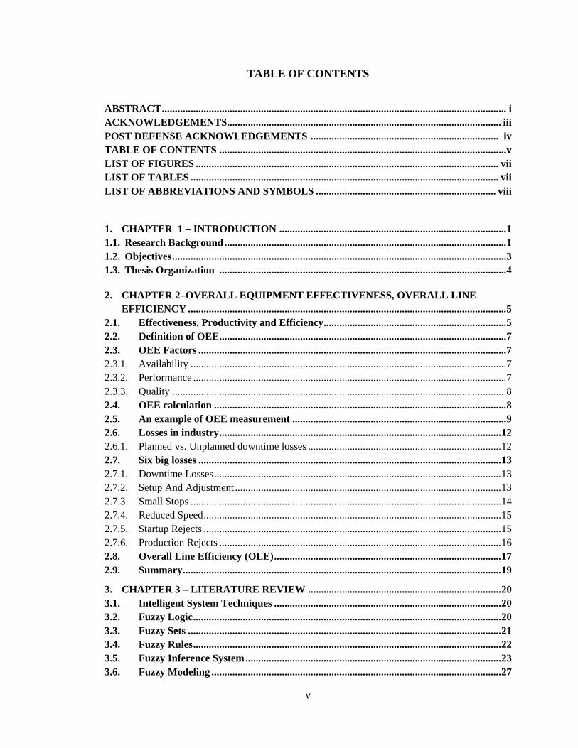
is doing things right” [6]. Figure 2-1 compares efficiency with effectiveness.
6
Doing the right things rightDoing the right things
Doing things Doing things right
Efficiency
Effe
ctiv
en
ess
low high
low
hig
h
Figure 2-1–Effectiveness vs. Efficiency [7].
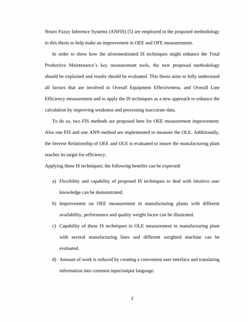
Table below illustrate the difference between mentioned terms.
Effectiveness Efficiency
Focuses on desired results Focuses on doing works in a
correct manner
End of task most important Resource to do a task is most
important
Anticipates changes Reacts to changes
Motivated toward growth Comfortable with keeping things
the way they are
Seeks success seeks to avoid failure
Table 2-1 - Effectiveness vs. Efficiency [8].

7
2.2. Definition of OEE:
Overall Equipment Effectiveness is a key performance indicator that can be
implemented to benchmark, analyze and improve a production process by measuring
inefficiencies and groups them in different categories [9]. In other words, OEE is total
utilization of time, material and facilities in a manufacturing process, [10].
2.3. OEE Factors
Overall equipment effectiveness is a calculation of the three following metrics:
2.3.1. Availability:
Availability is the ratio of actual production time that a machine is working
divided by the time the machine is available. Note that another methodology for
calculating availability could be shown as follows:
2.3.2. Performance:
Performance of a machine is the percentage of total number of parts on that
machine to its production rate. In simple words, performance measures the ratio of actual
operating speed of the equipment and the ideal speed [11]
Please note that ideal cycle time of a machine is the minimum cycle that can be
achieved in optimal conditions. It is also known as design cycle time.

8
2.3.3. Quality:
To gain insight into the quality aspect of a production process the quality portion
of OEE is defined. The Quality metric represents good (acceptable) units produced by
machine divided by the total units produced by that machine in the production time.
2.4. OEE calculation
OEE takes into account contributing factors and is calculated as follows:
Since all three factors involved in OEE calculation have a value between 0 and 1,
OEE itself varies between 0 and 100 per cent which makes OEE a severe test. For
example, if all three aforementioned factors are 90 percent, OEE would be 72.9%, [6].
Nakajima (1988) suggested the ideal values of OEE factors and corresponding OEE as
follows [12].
OEE factor Ideal Values
Availability 90%
Performance 95%
Quality 99%
OEE 85%
Table 2-2–World class OEE and its factors [12].

9
It is necessary to mention that other calculations are being used to calculate
availability, performance and quality. Some are mentioned here:
As it can be seen OEE factors are different in every manufacturing plant. World
class manufacturing with an active six sigma methodology may even reach a higher
quality rate. However, a worldwide average OEE rate in a production plant is 60%. [10]
2.5. An example of OEE measurement
A hypothetical manufacturing plant is assumed to have a shift length of 8.5 hours.
There are two short breaks, one in the morning and one in the afternoon and duration of
each of these short breaks is 15 minutes. Also, there is meal break at noon for 30
minutes. The company encountered a downtime due to the machine breakdown for 52
minutes and the ideal cycle time of product is 5 seconds. At the end of the shift 4000
pieces are produced whereas 96 pieces are rejected due to quality non-conformities. The
following table is a summarization of production data to be used for OEE calculation.

10
Item Data
Shift length 8.5 hours / 510 minutes
Short breaks 2 x 15 minutes
Meal break 30 minutes
Downtime 52 minutes
Cycle time 5 seconds
Total pieces 4000
Rejected pieces 96
Table 2-3– OEE measurement example‟s data.
Planned production time = shift length – breaks
=510-60
=450
Running time = planned production time – downtime
=450 – 52
= 398 min
Run rate = time /produced pieces
=60/5
=12 pieces per minute
Good pieces =total pieces – rejected pieces
=4000-96
=3904

11
Availability =running time/planned production time
=398/450
=0.884
Performance =total pieces/operation time/ideal run time rate
=4000/ (398/12)
=0.837
Quality =good pieces/total pieces
=3904/4000
=0.976
OEE =Availability x Performance x Quality
=0.884 *0. 837 * 0.976
=0.722

12
2.6. Losses in industry
The main goal behind OEE is to minimize and/or eliminate the inefficiency
causes in a manufacturing process. Normally, losses are considered as basic knowledge
for discussing OEE. Different categorizations of losses are explained next.
2.6.1. Planned vs. Unplanned downtime losses
Ericsson and Dahlén (1993) has divided the downtime in two groups, planned
stop and unplanned stop [13]. As mentioned, OEE concerns inefficiencies within planned
production time. Although “planned downtime losses” are considered as inefficiencies in
a manufacturing environment, the OEE is not affected by those losses.
The following events can be categorized as planned downtime
Authorized pauses
Not working days/weekends
Trainings/meetings during working hours
Scheduled downtime for product changes
Preventive maintenance/overall
Equipment modification
The figure below shows planned and unplanned downtime losses in a production time
Theoretical production time
Planned production time
Running time
Planned down time
Unplanned down time
Figure 2-2 – Planned/unplanned downtime [6].

13
2.7. Six Big Losses
The most common inefficiency causes in industry are those called “six big losses.” These
losses can be categorized in downtime losses, speed losses, and quality losses.
To find a way to monitor and improve a manufacturing process, six big losses are
addressed as follows.
2.7.1. Downtime losses
As previously mentioned, downtime is categorized as planned and unplanned
downtime, and eliminating unplanned downtime is a key to OEE improvement. In fact
downtime is the most important factor for equipment effectiveness improvement since
other metrics cannot be addressed if the manufacturing process is down. Tooling failures,
unplanned maintenance, equipment breakdowns are some examples of downtime losses.
2.7.2. Setup and Adjustment
Setup and adjustment losses occur when production of one item ends to produce item
equipment is adjusted [11].This is often a set of adjustments to machines and/or
equipment in order to produce a product that meets the standard requirements. Setup time
should be tracked in order to reduce this loss. Some programs such as Single Minute
Exchange of Die (SMED) are being used in industry to reduce this loss.
Warm up time and changeovers can be represented as setup and adjustment losses in
a manufacturing process.
14
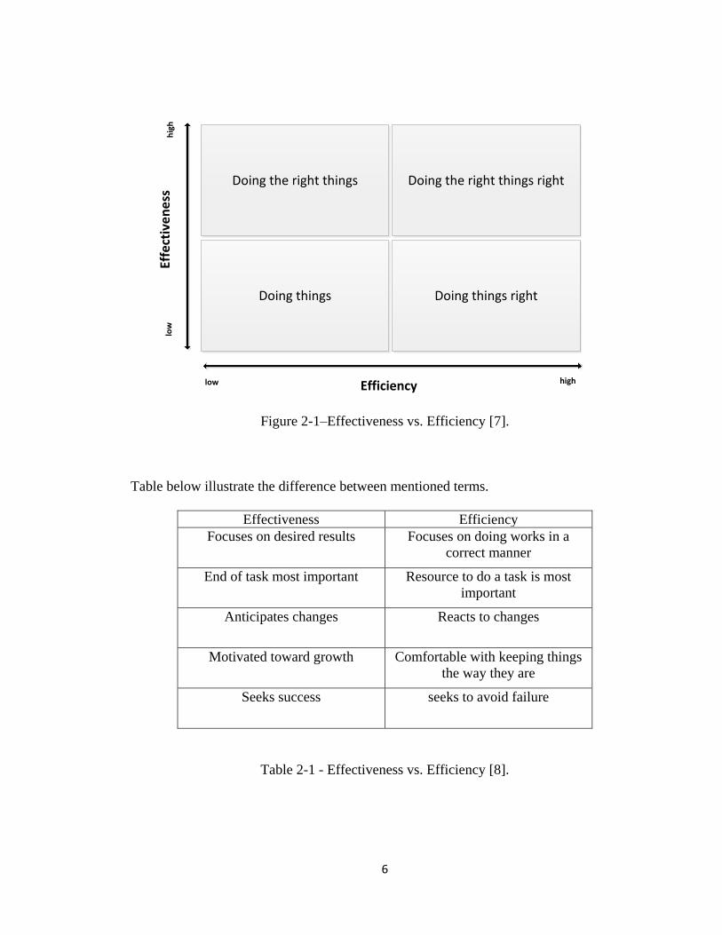
2.7.3. Small Stops
These stoppages occur when the machine stops due to a temporary problem such as
an activated sensor that shuts the machine down automatically. These minor stoppages
are usually less than 10 minutes and can be dealt with by the operator and generally there
is no need to call a maintenance team. These losses stand for 20-30 per cent of OEE in
most automated lines [14].
Component jams, sensor blocked and delivery blocked are categorized as small
stop losses. Inefficiencies due to small stops are shown in the following figure.
Figure 2-3 – Speed reduction due to small stops, [6].

15
2.7.4. Reduced Speed
Knowing the ideal cycle time of a machine and comparing it with the actual cycle
time, it will be possible to monitor low running or reduced speed losses. Machines may
run at the speed less than the ideal run rate for various reasons. Training level of
operators, worn equipment can be categorized as the aforementioned reasons.
2.7.5. Startup Rejects
Startup losses occur in the initial start of a machine up to the stabilization of its
products quality. A root cause analysis can be done to pinpoint the potential causes of
rejects and to prevent similar losses from occurring in the future. It is necessary to note
that reworks, scraps and incorrect assembly, all are considered as rejects in the
production processes.
Figure 2-4 –Quality losses due to startup and shutdown [6]

16
2.7.6. Production Rejects
This quality loss occurs in a steady-state production and is not attributed to start up.
Often a six-sigma program where the goal is to achieve zero defects is used to reduce
production reject losses while focusing on identifying and removing causes of rejects.
Damage, scraps, and reworks, are some examples of production reject losses.
The following figure illustrates different types of losses in a production process.
Theoretical production time
Avalable production time
Valuable operating time
Gross operating time
Net operating time
External losses
Down time losses
Speed losses
Quality losses
Availabality
Performance
Quality
Figure 2-5 – Losses in a manufacturing process, [6].
Significant improvement can be achieved within a short period by eliminating these
six losses in industry as a result of enhanced maintenance activities and equipment
management [15].

17
2.8. Overall Line Efficiency (OLE)
In a situation where a manufacturing line consists of unbalanced/decoupled
machines OEE alone is not sufficient [16]. Also OEE is measured for an isolated
individual equipment and controlling a single tool does not seem to be effective [17].
Overall Line Efficiency is a new concept in industry that shows how well a
manufacturing line is running compared to how well it could be running. This metric
evaluates the line performance in the production phase. Utilization of assets (in other
words OEE) is the most important metric for measuring Overall Line Efficiency.
However utilization of human resources needs to be covered.
For a manufacturing plant consists of a single production line and machines with
the same levels of importance (weight factor), OLE could be measured as an average of
all machines‟ OEE. However in most manufacturing plants various production lines such
as paint shop, assembly, weld, and fabrication with different weights are running. As an
example of OLE calculation and its complexity the following is explained: Two factories
are operating, one with a single production line with 3 machines as shown below:
A B C
Cycle time : 10 secOEE :81 %
Cycle time : 10 secOEE : 72 %
Cycle time : 10 secOEE : 84 %
Figure 2-6 – A manufacturing process with single production line.

18
As can be seen in the figure, all machines have the same cycle time and therefore
the same weight in production. In this case OLE can be measured as the average of OEEs
as follows:
The second factory has a more complex process with three manufacturing lines
and different weight of machines in each line. The figure below shows the process and
cycle time of each machine:
Figure 2-7 – A manufacturing process with different production lines and weight factors.

19
Since manufacturing lines of this factory are not balanced and bottle neck exists
in each line, OLE calculation is more complex.
2.9. Summary
In this Chapter, the traditional heuristic methods of OEE and OLE measurements,
as well as six big losses in industry have been explained. Moreover, the overall
weighting of equipment effectiveness is explained as a more accurate approach to OEE
measurement; however this method is not as quick as the user would expect. In addition,
in many cases the user may encounter uncertain data as inputs. For instance in some
cases cycle time, and therefore run rate, cannot be calculated.
These reasons led to IS techniques which are proposed here as a more efficient
method rather than the traditional heuristic method of OEE measurement. Also IS
techniques are used to measure the Overall Factory Efficiency in complex cases.
Chapter 3 is dedicated to a brief literature review on Fuzzy Inference System, and
Artificial Neural Networks, and their functionality.

20
CHAPTER 3 – LITERATURE REVIEW
This Chapter aims to explain some Intelligent Systems (IS) techniques that are
implemented in the proposed methodologies. Fuzzy Inference Systems (FIS), and
Artificial Neural Networks (ANN), are two IS techniques that are used in this research.
The following sections provide a brief explanation of these IS techniques that is extracted
from Neuro Fuzzy and Soft Computing [5].
3.1. Intelligent System Techniques
Knowledge, techniques, and methodologies, are combined in Intelligent Systems
to deal with complex real world problems [5]. It is advantageous to use various IS
techniques such as Fuzzy Logic and Artificial Neural Networks in a variety of problems.
Several of these IS techniques such as Fuzzy logic, Fuzzy Inference Systems and
Artificial Neural Networks are briefly explained below:
3.2. Fuzzy Logic
Fuzzy Logic is being widely used in modeling to manipulate information and also
in a diversity of real world problems [18], [5]. Transferring user language and/or
experience into a numerical value and providing satisfactory results based on imprecise
or uncertain data are some of the Fuzzy Logic‟s advantageous characteristics, [18]. It
concentrates on solving a problem based on if-then judgments rather than trying to model
a system automatically, [5].

21
3.3. Fuzzy Sets
Introduced by Zadeh [18] in 1965, “a fuzzy set is a class of objects with
continuum of grades of membership” which maps each member of the set to a
membership degree (truth value) from zero to one. Mathematically expressed “If is a
collection of objects denoted generically by , then a fuzzy set A in is defined as a set
of ordered pairs:
* ( )| }
Where ( ) is called the membership function (MF) for the fuzzy set A”, [5].
An example of a Fuzzy Set is as below:
Assume that a family is planning a trip by their own car and since the time is
limited, this family tends to choose a closer destination. Close can be represented as a
Fuzzy Set on a universe of distance and the following can be considered:
● Below 500 km, distance considered close and distance difference is not a factor of
decision making.
● Between 500 km to 1000 km, family tends to choose a closer destination.
● Between 1000 km to 1500 km, variation in distance makes a huge difference
between close and far destinations.
● Above 1500 km, family will not consider this option as its destination.
Considering the aforementioned explanation membership function of distance is shown
as follows:

22
Figure 3-1 - Membership function of distance.
3.4. Fuzzy Rules
“A fuzzy if-then rule (also known as fuzzy rule, fuzzy implication or fuzzy conditional
statement), assumes the form
If X is A then Y is B
Where A, B are linguistic values defined by fuzzy sets on universe of discourse X and Y
respectively. Often „X is A‟ is called antecedent or premise, while “Y is B” is called the
consequence or conclusion.”, [5].
If-then rule examples are widespread in our daily life such as the following:
If the road is foggy, then reduce the speed.
500 1000 1500
1
Distance (KM)

23
3.5. Fuzzy Inference System
A Fuzzy Inference System consists of three components: the fuzzier that converts
inputs to linguistic terms using the membership function; the inference engine that uses
if-then rules to convert fuzzy inputs to output(s); and the defuzzifier that extracts the
inference engine‟s fuzzy output to crisp outputs that best represent a Fuzzy Set. “With
the crisp input and outputs, a fuzzy inference system implements a nonlinear mapping
from its input space to its output space.” [5].
The figure below represents a Fuzzy Inference System:
Figure 3-2 - A Fuzzy Inference System.

24
Figure 3-3 – Fuzzy inputs to outputs conversion using if-then rules, [5].
According to literature, Neuro fuzzy and soft computing [5], there are three main Fuzzy
Inference Systems as follows:
● Mamdani Fuzzy Inference Systems
● Sugeno Fuzzy Inference Systems
● Tsukamoto Fuzzy Inference Systems
As mentioned, a defuzzification method is used to convert the fuzzy output to a crisp
output especially when a FIS is used as a controller. Five most common defuzzification
methods and their calculation of expected value are as follows, [5]:
Smallest of Max
Largest of Max

25
Mean of Max
∫
∫
Centroid of Area
∫ ( )
∫ ( )
Bisector of Area.
∫ ( ) ∫ ( )
The next figure shows the result for each defuzzification method.
Figure 3-4 – Expected value of different defuzzification methods, [5].
26
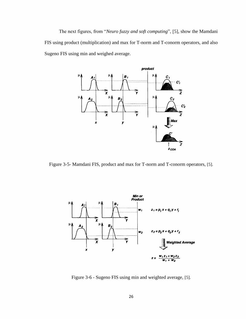
The next figures, from “Neuro fuzzy and soft computing”, [5], show the Mamdani
FIS using product (multiplication) and max for T-norm and T-conorm operators, and also
Sugeno FIS using min and weighed average.
Figure 3-5- Mamdani FIS, product and max for T-norm and T-conorm operators, [5].
Figure 3-6 - Sugeno FIS using min and weighted average, [5].

27
Please note that Tsukamoto FIS is mainly used in control problems where an
estimation of output exists. Hence this system is not applicable to the proposed
methodology for the OEE and OLE measurements and is not explained here.
3.6. Fuzzy Modeling
Generally speaking, an FIS is designed based on previous experience/behavior of
a target system and it is expected for the FIS to reproduce that behavior.
The process of constructing a Fuzzy Inference System, which is called Fuzzy Modeling,
offers the following advantages.
● Human knowledge is incorporated into the modeling process using the rule
structure of a FIS.
● Mathematical techniques also can be implemented for Fuzzy Modeling as in other
mathematical modeling methods.
Fuzzy modeling process can be performed in two stages: surface structure, and “deep
structure”; and each stage consists of the following tasks:
1. Surface structure
1.1.Selecting related inputs and outputs.
1.2.Choosing type of FIS.
1.3.Determining the order of consequent equation for Sugeno FIS and number of
linguistic terms associated with inputs and outputs.
1.4.Designing if-then rules.

28
2. Deep structure
2.1.Choosing suitable membership function (s).
2.2.Applying human experts to specify the membership function‟s parameters.
2.3.Refine the parameters using an optimization process, if necessary.[5]
Although the accuracy of a FIS can be tested by comparing the output of FIS and
the desired value of the potential answer; mathematical optimization methods can be
implemented off line to improve the accuracy of Fuzzy Inference Systems. For example,
let‟s assume a Fuzzy Inference System with three inputs( ), and two
outputs( ). Then, the outputs can be expressed as a function the inputs and of the
Membership Functions (MF) parameters of the Fuzzy Inference System. That is,
( ) ( )
In order to properly tune the FIS MF Parameters; it may be convenient to optimize
offline using a nonlinear optimization technique the following function;
( ) ( ) ( )
Where ( ) ‖ ̅‖ ; ̅ is a desired/estimated output
And ( ) represent a performance criterion, [19], on the FIS.
In the case that ̅ is not available; then, ( ) , and
( ) reduces to ( ). The optimization process may be done
several times for a series of different values of ( ). The result of the offline
optimization process will lead to a fine tuned FIS.

29
3.7. Artificial Neural Networks (ANN)
“ANN is a network structure consisting of number of nodes connected through
directional links. Each node represents a process unit, and the link between notes specify
the casual relationship the connected nodes. All or parts of the nodes are adaptive, which
means the output of these nodes depend on the modifiable parameters pertaining to these
nodes” [5] these parameters should be updated in order to minimize the measured error.
“This error is a mathematical expression that measures the discrepancy between
the network‟s actual output and a desired output.”[5] Also “each node in an adaptive
network performs a static mapping from its input(s) to output.”[5].
It is necessary note that functions of nodes can be varied due to facilitation of the
learning algorithm. “In particular, if we use the gradient vector in a simple steepest
decent method, the resulting learning paradigm is often referred to as the
backpropogation learning rule.”[5]
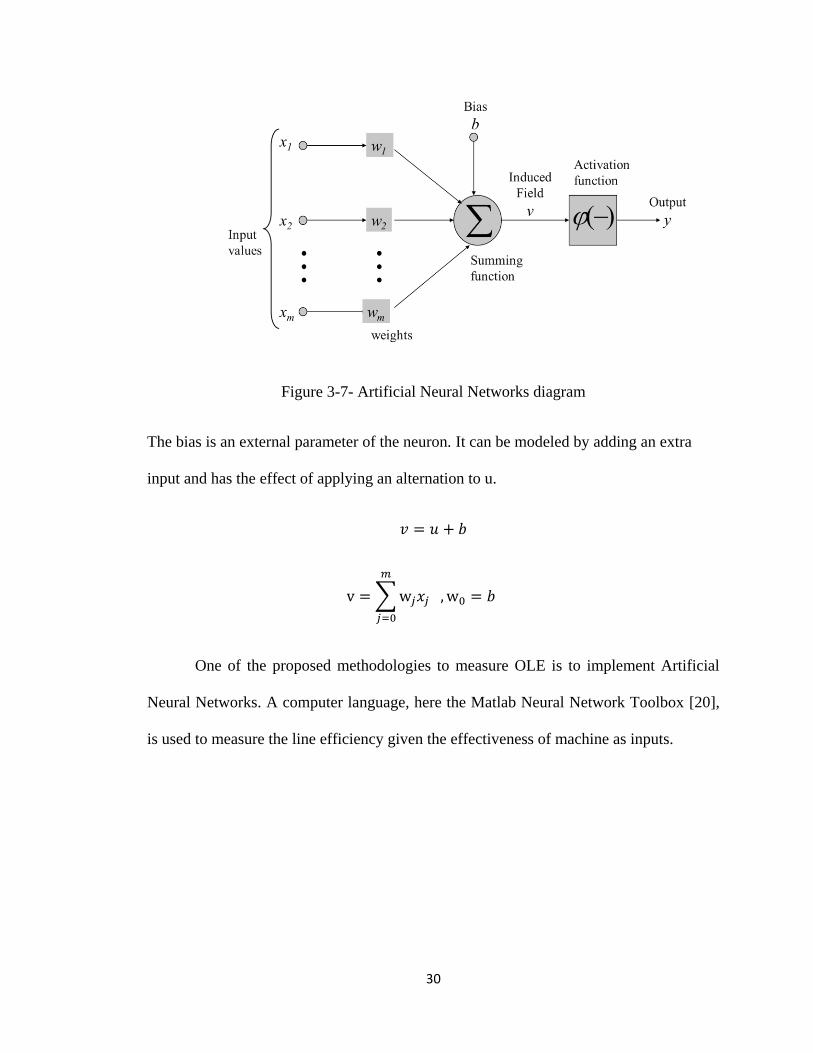
Figure 3-7 illustrates consistency of an artificial neural network:
A set of links, describing the neuron inputs, with weights: W1, W2 … Wm
A function for computing the weighted sum of the inputs as follows :
∑
A function for limiting the widespread outputs on the neurons: ( )
here b represents the bias
30
Figure 3-7- Artificial Neural Networks diagram
The bias is an external parameter of the neuron. It can be modeled by adding an extra
input and has the effect of applying an alternation to u.
∑
One of the proposed methodologies to measure OLE is to implement Artificial
Neural Networks. A computer language, here the Matlab Neural Network Toolbox [20],
is used to measure the line efficiency given the effectiveness of machine as inputs.
31
The following steps describe the process of Artificial Neural Networks to reach the
objectives:
a) Network design
Architecture of the ANN including the number of layers, number of nodes per
layer and structure of each node is determined in this step. Also the Learning
rules are selecting in this phase.
b) Network training
In this step, objectives are established to achieve the accuracy of new results.
Moreover, the network is validated through a separate test set and also the
maximum error rate is determined.
c) Data preparation
The quality of data has a severe impact on accuracy of result; so it is fair to say
this step is the most important one during the process. Cleaning data such as
removing exceptions and eliminating incomplete sets of data is also involved in
data preparation.
d) Post-training analysis
Visualization of the model through charts and graphical interfaces and sensitivity
analyses of inputs are counted as post-training analysis.

32
3.8. Summary:
Main purpose of explaining some of the IS techniques and their advantage is to
draw a picture of how aforementioned methodologies in this chapter are implemented to
measure the overall equipment effectiveness and overall line efficiency more accurately
The next chapter present implementation of mentioned IS techniques and their capability
of problem solving in OEE and OLE measurement.

33
CHAPTER 4 - METHODOLOGY
This Chapter presents three new methodologies for OEE measurement, and two
novel methods for OLE calculation based on IS techniques as proposed. Moreover, an
inverse relationship procedure using ANNs is implemented to specify the reduction of
losses to maintain a certain level of efficiency in a manufacturing plant. The IS
techniques proposed here have several advantages over traditional methods of OEE and
OLE calculation. Some benefits of implementing these IS techniques for OEE calculation
are mentioned below:
First, measurement can be done for all manufacturing plants in different
industries regardless of production process.
Different weight factors can be allocated to OEE factors involved in the
measurement depending on the process. For instance in aerospace or medical
equipment industry, quality may play a more important role in equipment
effectiveness measurement rather than the availability of equipment; therefore, a
higher weight can be allocated to quality factors of OEE.
Also implementing IS techniques to measure the Overall Line Efficiency offers several
advantages:
OLE can be measured for factories with a variety of production lines and
machines with various weight factors.
Efficiency can be maintained at a certain level when addressing the proper loss
reduction.

34
4.1. Approach with Fuzzy Inference Systems (FIS)
As it has been already mentioned, some of the new proposed methodologies for
OEE and OLE measurement are based on Fuzzy Logic. A computer language and/or an
interface, here the Matlab Fuzzy Logic Toolbox, is normally used to simulate a variety of
situations, and to consider parameters such as various inputs and outputs. It is important
to note that although in this thesis Matlab and its Fuzzy Toolbox as a computer language
and are used, other computer platform/interface such as fuzzyTECH can be implemented
for the proposed Fuzzy Inference System.
In order to achieve optimum results the following steps are proposed to describe
the Fuzzy Inference Systems process:
(a) Objective Definition: Specific goals can be defined to be reached after the
completion of the process. In this case, accurate OEE and OLE measurement
are the objectives.
(b) Environment observation: Observing the process and considering all inputs
and outputs, the weight factor of each parameter as well as choosing proper
membership functions are categorized in this step. For instance, in the OEE
measurement using FIS, considering quality losses with a higher weight or
adding energy consumption as another input can be achieved through
observation of environment.
(c) Setting rules: If-then rules must represent the interaction of inputs and
outputs in the real life system and are set by a system expert. Setting rules that
do not represent the system is a potential cause of inaccurate results.

35
(d) Proper FIS selection: Based on the process and objectives, different Fuzzy
Inference Systems such as Mamdani, Sugeno are being used to represent a
system more accurately.
(e) Performing actions: Once a Fuzzy Inference Systems model with inputs,
outputs and rules is defined, results can be obtained to specify the objectives.
4.1.1. Fuzzy Inference Model
The new proposed methodology presents a Mamdani Fuzzy Inference Model and
a Sugeno Fuzzy Inference Model, for the OEE and OLE measurements respectively.
Structures and details of these models such as rules, membership functions and
defuzzification methods are provided in Appendix A.
4.2. OEE Measurement Using Mamdani FIS
The Mamdani FIS is the first method presented in this thesis to measure the OEE
of a machine. In this method, availability, performance, and quality, are calculated based
on their associated losses involved in an equipment effectiveness reduction. Here a Fuzzy
Inference System assigns different qualifiers to the parameters and the Matlab Mamdani
FIS Toolbox is the interface that is used to simulate the process.
In order to complete the OEE measurement, six big losses in industry are
considered as inputs of the system. As mentioned in Chapter 2 of this thesis;
breakdowns, and setup and adjustment are two losses associated with the availability
factor. Small stops and reduced speed cause inefficiency and performance reduction.
Finally startup and process rejects are quality losses that are involved in overall

36
equipment effectiveness. Given the six losses as inputs, the OEE of the machine is the
single output of Mamdani Fuzzy Inference System.
Inputs of Mamdani FIS and their values are explained in detail as follows:
1. Breakdowns
Breakdowns can get values as [low; average; high], depending on the process. This
loss has one of the biggest impacts on OEE; because if a machine does not operate,
there will not be running time and therefore no other losses can be observed.
2. Setup and Adjustment
Setup and Adjustment is also associated with availability factor in OEE and get
values as [low; average; high]
3. Small Stops
Small stops affects the performance factor and get values of [low; average; high]
depends on the process and operator prospective.
4. Reduced Speed
This input is also related to performance factor and values of [low; average; high] can
be assigned to it.
5. Startup Rejects
This quality loss has one of the following values: [low; average; high]

37
6. Process Rejects
Depending on the manufacturing process, and the applied quality system; process
rejects can affect the OEE severely. Values of [low; average; high] can be assigned to
this input as well.
Please note that all inputs can get higher range qualifiers in this method. For
instance in the aerospace industry, due to its sensitivity, speed losses may have values
of [low; high] whereas the set [very low; low; average; high; very high] is allocated
to quality losses. Also other inputs such as environmental pollution or energy
consumption can be taken into account for measuring the equipment effectiveness.
Overall Equipment Effectiveness (OEE) is the only output of the system, given six
big losses (and other potential losses in the production process) and their associated
weight factors. To obtain a more accurate rule setting and therefore more accurate
results, values of [very low; low; average; high; very high] can be assigned to OEE.
Once inputs and output of the system are determined, the next step for the system
to reach its goal is to set antecedent-consequent (if-then) rules. Like determining
inputs and outputs, operator experience/knowledge plays an important role in this
step by applying weight factors to each input into the system. Setting inaccurate rules
has a big negative impact on results. The If-then rules for this Fuzzy Inference
System are provided in Appendix B Section 1.

38
Mamdani Fuzzy model to measure the OEE is shown in figure below:
LOW
AVERAGE
HIGH
BREAKDOWN
SETUP & ADJUSTMENT
REDUCED SPEED
STARTUP REJECT
PRODUCTION REJECT
SMALL STOP
MAMDANI FIS
IF-THEN RULES,
Defuzzification Methods
OEE
Figure 4-1 – OEE measurement using Mamdani FIS.
4.3. OEE Measurement Using Sugeno FIS
A typical fuzzy rule which is generated from a given input-output data set in
Sugeno model has the following form:
( )
Given that, Sugeno FIS is implemented to measure OEE in processes that weight factor
of inputs can be described in coefficients of an equation. For instance if all associated
inputs of OEE measurement (six big losses) have the same weight factor OEE can be
presented as follows:
This can be modeled as a first order Sugeno fuzzy model.

39
In the second case, the quality factor has a severe impact on OEE; so the Sugeno fuzzy
Inference System can be modeled with more concentration on quality losses as follows:
( ) ( )
Since the Sugeno fuzzy model has six big losses as inputs and the OEE as output
of the system, and these parameters have been already considered in the Mamdani FIS in
this Chapter, no further explanation is presented here for each parameter.
Inputs:
1) Breakdowns: [low; average; high]
2) Setup & Adjustments: [low; average; high]
3) Small Stops: [low; average; high]
4) Reduced Speed: [low; average; high]
5) Startup Rejects: [low; average; high]
6) Process Rejects: [low; average; high]
Output:
1) OEE: [low; average; high]
As noted before, other inputs may be taken into account in OEE measurement
depending on the process. Environmental effects and energy efficiency are examples of
other potential inputs. Fuzzy if-then rules are available at Appendix B Section 2.

40
Sugeno Fuzzy Model to measure OEE is shown in figure below:
LOW
AVERAGE
HIGH
BREAKDOWN
SETUP & ADJUSTMENT
REDUCED SPEED
STARTUP REJECT
PRODUCTION REJECT
SMALL STOP
SUGENO FIS
IF-THEN RULES,
Defuzzification Methods,
OEE Membership Functions,
OEE = f (inputs)
OEE
Figure 4-2 – Sugeno FIS for OEE measurement.
4.4. Overall Line Efficiency (OLE) Measurement Using Mamdani FIS
Overall Line Efficiency is an important key performance indicator that monitors
how good a manufacturing line is running compared to how good it could be running. As
mentioned earlier in this Chapter, Overall Equipment Effectiveness is one of the most
powerful tools to measure the equipment utilization; so OLE can be calculated, taking
into account each machine‟s OEE in the manufacturing line.
Due to complexity of OLE calculation in a manufacturing line with different
types of machines, different cycle times, and also different weigh factors; Fuzzy
Inference Systems are proposed here to measure the Overall Line Efficiency.
In this method, the effectiveness (OEE) of every single machine in the manufacturing
line is an input into the system, and OLE can be designated as the output of the system.
41
The inputs and the output of this Mamdani FIS with their qualifiers are presented as
follows:
Inputs of Mamdani FIS for OLE calculation:
OEE machine1 = [low; average; high]
OEE machine2 = [low; average; high]
OEE machine3 = [low; average; high]
Output of Mamdani FIS for OLE calculation:
Overall Line Efficiency (OLE) = [very low; low; average; high; very high]
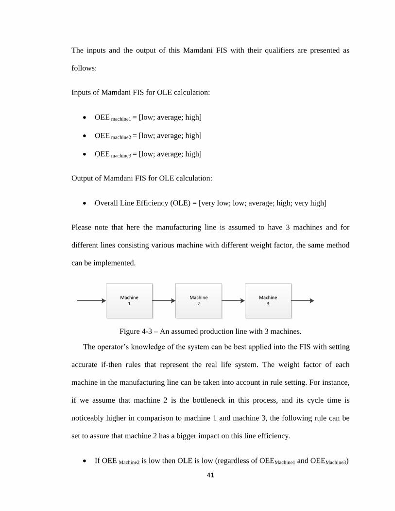
Please note that here the manufacturing line is assumed to have 3 machines and for
different lines consisting various machine with different weight factor, the same method
can be implemented.
Machine1
Machine2
Machine3
Figure 4-3 – An assumed production line with 3 machines.
The operator‟s knowledge of the system can be best applied into the FIS with setting
accurate if-then rules that represent the real life system. The weight factor of each
machine in the manufacturing line can be taken into account in rule setting. For instance,
if we assume that machine 2 is the bottleneck in this process, and its cycle time is
noticeably higher in comparison to machine 1 and machine 3, the following rule can be
set to assure that machine 2 has a bigger impact on this line efficiency.
If OEE Machine2 is low then OLE is low (regardless of OEEMachine1 and OEEMachine3)

42
LOW
MEDIUM
HIGH
OEEMachine1
OEEMachine3
OEEMachine2
MAMDANI FIS
IF-THEN RULES,
Defuzzification Methods
OLE
Figure 4-4 – OLE Mamdani Fuzzy Model
Fuzzy if-then rules are available at Appendix B Section 3.
Similarly, the Sugeno Fuzzy Inference System can be implemented for
calculating the OLE using a first or second order equation that specifies each machine‟s
contribution in the line efficiency.
43
4.5. Approach with Artificial Neural Networks (ANNs)
One of the proposed methodologies to measure OLE is to implement Artificial
Neural Networks. A computer language, here the Matlab Neural Network Toolbox, is
used to measure the line efficiency given the machine‟s effectiveness as input.
The following steps describe the process of Artificial Neural Networks to reach the
objectives:
e) Network design
Architecture of the ANN including the number of layers, number of nodes per
layer and structure of each node is determined in this step. Also the learning rules
are selected in this phase.
f) Network training
In this step, objectives are established to achieve the accuracy of new results.
Moreover, the network is validated through a separate test set and also the
maximum error rate is determined.
g) Data preparation
The quality of data has a severe impact on accuracy of result; so it is fair to say
this step is the most important one during the process. Cleaning data such as
removing exceptions and eliminating pairs with missing data is also involved in
data preparation.

44
h) Post-training analysis
Visualization of model through charts and graphical interfaces and sensitivity
analyses of inputs are counted as post-training analysis.
4.6. OLE Measurement Using Artificial Neural Networks
As it has been previously mentioned in Chapter 3, one of the greatest advantages
of ANNs is their ability to learn which is perceived from observed data in a function
approximation mechanism.
Since Overall Line Efficiency measurement can be very complex for different
manufacturing processes where traditional methods and calculations are not able to
achieve accurate results, it can be measured with Artificial Neural Networks. However it
is necessary to notice that ANNs can perform the measurement only if previous data exist
from other IS techniques, in other words results cannot be achieved before training the
Artificial Neural Networks using existing data.
In this method, after training the network using a set of machine‟s OEE (inputs)
and the OLE (output), a new set of inputs can be given to the trained Artificial Neural
Networks and corresponding OLE is extracted as its output.
Inputs and corresponding output of the neural network are presented as below:
Input 1 : * … +
Input 2 : * … +
Input 3 : * … +

45
Corresponding output: * … +
Note that in the assumed production line there are three machines with different weight
factors. Figure below shows the input and output of the neural network:
OEEMachine1 OEEMachine3OEEMachine2
OLE
Figure 4-5 – An assumed manufacturing line with 3 machines.
Having obtained inputs and output from the Fuzzy Inference System, the
architecture of the network is established with a number of layers and number of nodes in
each layer, also the maximum error is defined and ANN1 is trained. After training the
ANN1, new data (each machine‟s OEE) are given to the system and new output (OLE)
results. The next step is to validate and test the data with a separate set of inputs and
output.
Matlab Neural Network codes and initial data obtained from Fuzzy Inference
Systems including inputs (OEEs) and corresponding output (OLE) are provided in
Section 1 Appendix C.

46
4.7. Inverse Relationship in Artificial Neural Network for OLE Improvement
Companies and manufacturers use different methodologies such as Strengths,
Weaknesses, Opportunities, and Threats matrix (SWOT) to determine objectives and
allocate their resources to achieve those objectives at a certain period of time. Equipment
utilization is one of the most important factors that manufacturers seek to enhance to be
able to compete in current economic conditions. To maintain or improve the efficiency
level of a manufacturing line, it is necessary to specify which machines or equipment
need to be focused on in a complex process. For instance if the manager of a factory
decides to improve the press shop efficiency 20 percent, it is important to know which
machine needs to receive resources, also it is beneficial to know the impact of one
machine‟s OEE on Overall Line Efficiency.
Inverse relationship in Artificial Neural Network is proposed here to solve this
problem. Having obtained inputs and output from Fuzzy Inference System, the network
architecture is established with the number of layers and the number of nodes in each
layer, also the maximum error is defined and the artificial neural network 1 is trained.
Inputs and corresponding output of the neural network are presented as below:
Input 1 : * … +
Input 2 : * … +
Input 3 : * … +
Corresponding output: * … +

47
Next, new data (here OLE) is given to ANN 2 and it is simulated to achieve the
results. Inverse relationship for efficiency improvement is shown in figure below:
ANN2
OEEMachine1*
OEEMachine2*
OEEMachine3*
OLE*
Figure 4-6 –Artificial Neural Network Inverse relationship for OEE & OLE correlation.
Since an Artificial Neural Network with one input and multiple outputs has
infinite number of results, to limit the number of potential answers of each node and
therefore to improve the accuracy of the neural network‟s results, two more inputs are
created and added to the system as follows:
[
]
[
]
Note that minimizing these values, OEE of each machine and also efficiency of
the plant will be maximized. Having two new inputs, a new Artificial Neural network can
be illustrated as follows:
ANN2
OEEMachine1*
OEEMachine2*
OEEMachine3*
OLE*
y1
y2
Figure 4-7 – Artificial Neural Network Inverse relationship with3 inputs and 3 outputs.

48
The OEE of each machine is calculated as a result of inverse relationship of
Artificial Neural Network as follows:
( ) ( )
4.8. Summary
In this chapter two new methods using Fuzzy Inference Systems (FIS) have been
proposed for measuring the Overall Equipment Effectiveness. Also Overall line
Efficiency is measured with both Mamdani Fuzzy Model and the Artificial Neural
Networks.
At the end of this Chapter an inverse relationship procedure using Artificial
Neural Networks has been proposed as a tool for improving the efficiency in a
manufacturing line.
The next Chapter is dedicated to presenting the results from simulating different
scenarios proposed in this Chapter. Practical results in a case study along with figures of
simulation as well as a summary of advantages and recommendation for future work are
presented in the next chapter.

49
CHAPTER 5 - EXPERIMENTAL RESULTS
This Chapter presents the results from the proposed IS techniques
implementations which have been mentioned in Chapter 4. The results of each method
are analyzed considering different scenarios.
First, the OEE is measured with a Mamdani type of Fuzzy Inference System
(FIS) and the results are analyzed to test the accuracy of this method. Moreover, OEE is
measured implementing a Sugeno FIS, considering different weight factors and the
obtained results are analyzed. Also, the Overall Line Efficiency (OLE) is measured using
a Mamdani type of Fuzzy Inference System (FIS) and an Artificial Neural Network
(ANN). The results obtained are analyzed and compared to prove the accuracy of
aforementioned methodologies. Finally, the OEE is estimated taking into account of a
certain level of OLE using an inverse relationship from an Artificial Neural Network.
Chapter 5 is organized as follows:
a) Implementation of proposed methodologies in Chapter 4 and obtaining practical
results.
b) Analyzing obtained results from different scenarios.
c) Summary.

50
5.1. Fuzzy Inference Models:
The Matlab software and its Fuzzy Logic Toolbox have been used to implement the
proposed Mamdani and Sugeno FIS‟s mentioned in Chapter 4. Further detail on the
Fuzzy Logic Toolbox operation is provided in Appendix A.
A Mamdani fuzzy inference model to measure OEE, as previously explained, is
shown in figure 4-1. As it has previously mentioned, this FIS has six big losses in
industry as inputs to the system, and OEE is its sole output. After defining inputs and the
output of the Mamdani FIS, the Overall Equipment Effectiveness is measured according
to if-then rules, given the value of inputs. The surface plots of combination of inputs are
provided in Appendix C.
The second FIS model to measure the OEE is a Sugeno FIS which is illustrated in the
figure 4-2. Although the inputs and the output of this system are the same as Mamdani
FIS mentioned earlier; however in this case the Sugeno FIS can be used in processes
where a weight factor can be allocated to inputs. In other words, an equation can
represent the contribution of inputs to the system. Corresponding if-then rules and
surface plot with different combination of inputs are presented in Appendix B.
The last fuzzy model to be presented in this thesis is a Mamdani FIS to measure
Overall Line Efficiency (OLE) in a manufacturing plant. To avoid complexity a simple
manufacturing line with three machines is considered here. Please note that same
methodology can used for different processes with various numbers of machines and
more complex manufacturing lines.

51
Mamdani Fuzzy Model to measure OLE is shown in figure 4-4. As it can be seen
in the figure, the machines‟ OEEs are the inputs, and the OLE is the sole output of the
system. The corresponding if-then rules are presented further in Appendix B, section 3
and surface plots are provided in Appendix C.
5.2. Artificial Neural Networks
Matlab software and its Neural Network Toolbox have been used to implement
the proposed ANNs methodologies for OLE measurement. Further detail on the Neural
Network Toolbox Matlab code is provided in Appendix E.
As it has been previously mentioned, in this methodology the OLE is measured
after the ANN is trained and tested. The figure (5-4) shows the process of OLE
measurement by implementing an Artificial Neural Network.
ANN1
ANN1
OEEMachine1
OEEMachine2
OEEMachine3
OLE
OLE*
OEEMachine1*
OEEMachine2*
OEEMachine3*
Figure 5-1 - OLE Measurement using an ANN.

52
Also an Inverse Relationship of Artificial Neural Networks has been
implemented to calculate the OEE of each machine, given the OLE of that line. Figure
4-7 illustrates the Inverse Relationship of Artificial Neural Networks to calculate the
corresponding OEE, given the OLE.
5.3. OEE and OLE Measurement Experimental Results
As it has been previously mentioned, different scenarios are presented for each
method. First, common situations in industry are considered and values of inputs are
given to the system and the OEE and OLE are obtained. Also, the considered scenarios
are compared to demonstrate the accuracy of the proposed methodologies. A brief
explanation of each scenario along with a table of inputs and results is presented in this
Chapter. Please note that these methodologies can be implemented for various production
systems regardless of manufacturing process and variation of inputs to obtain
corresponding results.

53
5.3.1. OEE Measurement Using Mamdani FIS (Intelligent System 1)
Scenario#1
A machine in a manufacturing plant has been selected and its OEE is to be measured.
Assume there are qualitative losses associated with this machine in the past month;
however, its performance rate is average and also the machine was available to operate
properly (no major downtime) in this period. Therefore the following assumptions are
considered:
- Although a minor breakdown happened in this period; the machine was running
continually and its operator considers the value of breakdown loss as low.
- There were not setup and adjustment losses involved with the machine, and these
losses are considered to be low.
- Within the last month small stops occurred during running time and have been
fixed by the operator so small stops loss is considered average for this machine.
- Machines‟ ideal cycle time for pressing the metal part is 12 seconds however its
actual cycle time is measured as 15 seconds and reduced speed loss has
considered average by operator.
- There was not a considerable amount of startup rejects and this loss considered
low in this period.
- Qualitative issues have been observed and noticeable number of non-conforming
parts has been produced by this machine within last month. Therefore the process
reject loss is considered to be high is this period.

54
- In this manufacturing plant the availability factor has a higher weight factor rather
than performance and quality due to the short cycle time and inexpensive
material. Also, the Total Productive Maintenance (TPM) and Single Minute
Exchange of Die (SMED) are being implemented to increase the running time of
machines and reduce the setup and adjustment time.
The following Table presents the results considering the aforementioned parameters as
inputs of Mamdani FIS to measure OEE:
Table 5-1 - Experimental Result of Scenario #1.
As it can be seen from the table, given the aforementioned values as inputs and
weight factors, the corresponding OEE has been obtained as 74.8%. Note that, in
traditional methods of OEE calculation, the result, which is the average of inputs, is
69.67%.
Input
Parameters
Linguistic
Term Input Value
Output
Parameters
Output
Linguistic
Term
Deffuzified
Output
Value
Breakdown Low 15
OEE High 74.8
Setup &
Adjustment Low 10
Small Stops Average 38
Reduced
Speed Average 36
Startup
Rejects Low 18
Process
Rejects High 65

55
Scenario#2
A different machine has been selected in the same manufacturing plant and the following
assumptions are considered:
- Several major breakdowns have been occurred in past month and reduced the
availability of this machine. The operator considers the breakdown loss high.
- The Single Minute Exchange of Die (SMED) method was not effective for this
machine, as the setup time has increased significantly in this period. The setup
and adjustment loss is considered to be average.
- Small stops have occurred within this period, and the operator supposes this loss
as average.
- The actual cycle time of the machine is close enough to its ideal cycle time so the
reduced speeds loss is low.
- No major qualitative issue has been observed in this period, and both startup
reject and process reject losses are considered low.
- In this manufacturing plant the availability factor has a higher weight factor rather
than performance and quality due to the short cycle time and inexpensive
material. Also, the Total Productive Maintenance (TPM) and Single Minute
Exchange of Die (SMED) are being implemented to increase the running time of
machines and reduce the setup and adjustment time.

56
Given the assumptions above, the corresponding results are shown in the following table:
Table 5-2-Experimental result of Scenario #2.
It is important to note that value of each input in scenario 1 are assigned to a
different input value in scenario 2 to give a better understanding and ability to compare
between two scenarios. Observing from comparison of two scenarios, although the
average of both inputs is equal; however, the OEE has resulted in a reduced value in the
second case due to more weight factor of breakdown and setup and adjustment losses.
Input
Parameters
Linguistic
Term Input Value
Output
Parameters
Output
Linguistic
Term
Deffuzified
Output
Value
Breakdown High 65
OEE High 63.4
Setup &
Adjustment
Average 38
Small Stops Average 36
Reduced
Speed
Low 10
Startup
Rejects
Low 15
Process
Rejects
Low 18

57
5.3.2. OEE Measurement Using Sugeno FIS
Sugeno Intelligent System 1
Three pneumatic presses (scenarios) are assumed in a manufacturing plant and their OEE
are to be measured using a Sugeno FIS.
Following assumptions are considered as inputs to the Sugeno FIS system:
- Due to its material price, quality losses must be identified and reduced in this
manufacturing plant.
- Qualitative loss costs are drastically more than other losses associated with OEE.
In order to measure the OEE more accurately this company decided to assign
different weight factors to inputs. Table below shows the weight factor for each input, the
value of each input for these scenarios, and also the obtained OEE for each scenario.
Input Weight Factor Scenario 1 Scenario 2 Scenario 3
Breakdown 2 14 32 8
Setup & Adjustment 1 8 4 6
Small Stops 1 31 28 31
Reduced Speed 1 17 11 21
Startup Rejects 3 9 26 6
Process Rejects 4 77 12 8
OEE 65.08% 80.58% 89.67%
Table 5-3 - Experimental result of Sugeno Intelligent System 1.

58
Sugeno Intelligent System 2 (with 7 inputs)
Assume three industrial furnaces in a petrochemical plant and its OEE is to be measured
using a Sugeno FIS.
Following assumptions are considered as inputs to the Sugeno FIS system:
- Due to its energy costs, power consumption is associated in this machine‟s OEE.
- Availability factors affect the OEE drastically, so OEE will be low if machine is not
available (Availability losses are high), regardless of other OEE factors.
- Small stops may cause the batch to be ruined and an overhaul is necessary to clean
and run the furnace. So this loss has a very high weight factor in compare to other
losses.
In order to measure the OEE more accurately this company decided to assign
different weight factors to inputs. Table below shows the weight factor for each input, the
value of each input for each scenario, and also the obtained OEE for them.
Input Weight Factor Furnace 1 Furnace 2 Furnace 3
Breakdown 2 68 11 13
Setup & Adjustment 2 14 7 14
Small Stops 6 7 27 14
Reduced Speed 1 5 9 12
Startup Rejects 1 0 0.25 5
Process Rejects 1 0 2 1
Energy Consumption 1 25 33 37
OEE 26.1% 82.6% 89.4%
Table 5-4 - Experimental result of Sugeno Intelligent System 2.

59
5.3.3. OLE Measurement Using Mamdani FIS:
Mamdani Intelligent System 1
A manufacturing line is assumed with three different machines. Each machine
contributes in Overall Line Efficiency; however, the machine 2 is the bottleneck on this
line and plays a more important role in the OLE measurement. Therefore, the operator
uses his/her knowledge to set rules in the Mamdani FIS in order to measure the OLE
more efficiently. Also it is necessary to note that this technique can be used for any type
of manufacturing line with a variety of machines to measure its efficiency.
The following Table provides experimental results obtained for different scenarios
(represented each by a row) from the Mamdani FIS:
Scenario OEEmachine1 OEEmachine2 OEEmachine3 OLE
1 0.68 0.75 0.69 0.639
2 0.97 0.84 0.76 0.749
3 0.81 0.62 0.69 0.656
4 0.81 0.77 0.7 0.68
5 0.89 0.53 0.76 0.656
6 0.85 0.85 0.56 0.703
7 0.74 0.81 0.74 0.676
8 0.79 0.84 0.61 0.692
Table 5-5 - OLE Measurement, Mamdani Intelligent System 1 Experimental Results.

60
Intelligent System 2 (different weight factors from IS-1)
In this scenario a manufacturing line with 3 machines has been selected and its
OLE is to be measured using Mamdani FIS. Machine 1 has the highest cycle time among
other machines and is the bottleneck of this line. Machine 2 has a higher cycle time
rather than machine 3 and plays a more important role in OLE.
The following Table provides experimental results obtained for different scenarios
(represented each by a row) from the Mamdani FIS:
Scenario
OEEmachine1
(input1)
OEEmachine2
(input2)
OEEmachine3
(input3)
OLE
(output)
1 0.68 0.75 0.69 0.637
2 0.97 0.84 0.76 0.75
3 0.81 0.62 0.69 0.667
4 0.81 0.77 0.7 0.681
5 0.89 0.53 0.76 0.694
6 0.85 0.85 0.56 0.717
7 0.74 0.81 0.74 0.676
8 0.79 0.84 0.61 0.698
Table 5-6- OLE Measurement, Mamdani Intelligent System 2 Experimental Results.

61
Intelligent System 3 (4 inputs, two Machines in parallel)
In this scenario an assembly line with 4 machines is assumed and its OLE is to be
measured using Mamdani FIS. Press 2 has the highest cycle time among other machines;
however, Press 3 can perform the same task as Press 2 and they work in parallel. Press 1
and press 4 have equal weight factors.
Press 1Cycle time :38s
Press 2Cycle time :57s
Press 3Cycle time :52s
Press 4Cycle time :38s
Figure 5-2 – 4 presses in an assembly line and their cycle times.
Parallel Operation of two presses can be contributed in OLE measurement with setting if-
then rules such as: “If OEEPress2 AND OEEPress3 are hi then OLE is low”. The following
Table provides experimental results obtained for different scenarios (represented each by
a row) from the Mamdani FIS:
Scenario OEEPRESS1
(Input 1)
OEEPRESS2
(Input 2)
OEEPRESS3
(Input 3)
OEEPRESS4
(Input 4)
OLE
(Output)
1 0.87 0.70 0.68 0.81 0.592
2 0.97 0.84 0.88 0.76 0.705
3 0.856 0.841 0.792 0.795 0.692
4 0.811 0.56 65 0.795 0.541
5 0.735 0.72 0.562 0.49 0.521
Table 5-7 - OLE Measurement, Mamdani Intelligent System 3 Experimental Results.

62
5.3.4. OLE Measurement Using Artificial Neural Networks:
As it has been previously mentioned, an ANN is being used when a set of inputs
and corresponding outputs are available in the system. Giving existing data to the Neural
Network, the new outputs (OLE) can be obtained from a set of new inputs (OEEs).
Artificial Neural Network is being discussed in this thesis for the following reasons:
a) Approaching a new technique to measure OLE in a production process with
existing data.
b) Implementing an inverse relationship to calculate OEE of each machine given
Overall Line Efficiency (OLE).
In the following example the OEE has been measured 100 times with the Mamdani FIS
given each machines‟ OEE as inputs and OLE as output of the system. An ANN1 has
been trained using these data and a new OLE has obtained given a new set of machines‟
OEE. The following table compares the obtained OLE from Mamdani FIS and the ANN1
technique from the Matlab code in Appendix B for different scenarios (each row):
Scenario Obtained OLE using Mamdani FIS Obtained OLE using ANN1
1 73.896 73.8852
2 74.504 74.5080
3 73.544 73.5333
4 68.936 68.9358
5 72.466 72.3953
6 71.328 71.3192
Table 5-8 - Obtained OLE from Mamdani FIS and ANN1 comparison for different
scenarios
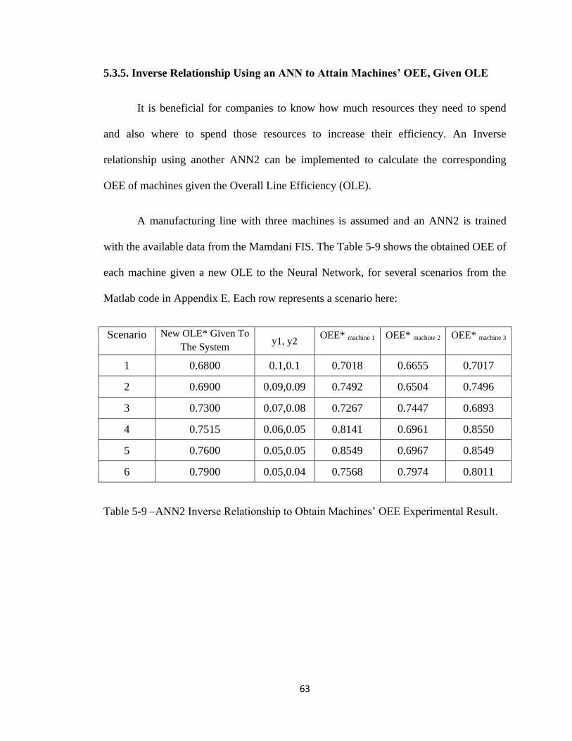
63
5.3.5. Inverse Relationship Using an ANN to Attain Machines’ OEE, Given OLE
It is beneficial for companies to know how much resources they need to spend
and also where to spend those resources to increase their efficiency. An Inverse
relationship using another ANN2 can be implemented to calculate the corresponding
OEE of machines given the Overall Line Efficiency (OLE).
A manufacturing line with three machines is assumed and an ANN2 is trained
with the available data from the Mamdani FIS. The Table 5-9 shows the obtained OEE of
each machine given a new OLE to the Neural Network, for several scenarios from the
Matlab code in Appendix E. Each row represents a scenario here:
Scenario New OLE* Given To
The System y1, y2
OEE* machine 1 OEE* machine 2 OEE* machine 3
1 0.6800 0.1,0.1 0.7018 0.6655 0.7017
2 0.6900 0.09,0.09 0.7492 0.6504 0.7496
3 0.7300 0.07,0.08 0.7267 0.7447 0.6893
4 0.7515 0.06,0.05 0.8141 0.6961 0.8550
5 0.7600 0.05,0.05 0.8549 0.6967 0.8549
6 0.7900 0.05,0.04 0.7568 0.7974 0.8011
Table 5-9 –ANN2 Inverse Relationship to Obtain Machines‟ OEE Experimental Result.

64
To confirm the accuracy of inverse relationship from the ANN2; the outputs of
the ANN2 (OEE* machine 1, OEE* machine 2, OEE* machine 3) are given to the ANN1 and
corresponding OLE is extracted and compared to given OLE* as an input to the ANN2.
Following table illustrate the comparison between OLE* in ANN2 and Obtained OLE in
ANN1:
Given OLE*
to ANN2
OEE* machine 1 OEE* machine 2 OEE* machine 3
Obtained OLE
from ANN1
MSE
0.6800 0.7018 0.6655 0.7017 0.68363 1.31E-05
0.6900 0.7492 0.6504 0.7496 0.6999 9.80E-05
0.7300 0.7267 0.7447 0.6893 0.72635 1.33E-05
0.7515 0.8141 0.6961 0.8550 0.76533 1.91E-04
0.7600 0.8549 0.6967 0.8549 0.7758 2.50E-04
0.7900 0.7568 0.7974 0.8011 0.78818 3.33E-06
Table 5-10 –Given OLE* to ANN2 and obtained OLE from ANN1 comparison.
From the Table 5-10, it can be easily observed that the ANN2 results are quite
accurate.

65
5.4. Summary
In this Chapter many scenarios have been assumed for each Intelligent System to
measure the OEE and the experimental results have been obtained. It is necessary to
mention that proposed methodology can be implemented in every production process
regardless of its product and complexity. Also other inputs may be taken into
consideration depending on the manufacturing process.
Moreover, the Overall Line Efficiency (OLE) has also been measured using a
Mamdani Fuzzy Inference System and an Artificial Neural Network for manufacturing
lines where weight factors of machines are not equal and the average of machines‟ OEE
cannot represent the Line Efficiency. Also in this case for each developed Intelligent
System many scenarios have been considered. The obtained results from the Mamdani
FIS are compared with the results from the ANN and both results are very close.
Last, an Inverse Relationship has been implemented to obtain the corresponding
OEE, given the Overall Line Efficiency (OLE), and many scenarios have been
considered. This proposed methodology can be used to perform a sensitivity analysis on
machines‟ OEE and assign resources to machines where OLE can be improved more
effectively.

66
CHAPTER 6 – CONCLUSION
This thesis aims to propose new approaches and methodologies to measure the
Overall Equipment Effectiveness and Overall Line Efficiency implementing Intelligent
Systems (IS) techniques such as Fuzzy Inference System and Artificial Neural Networks.
To accomplish this purpose the IS techniques are fully evaluated and the effectiveness of
these methodologies is tested assuming common scenarios in industry and analyzing the
experimental results. This thesis is organized as follows:
- First, the Overall Equipment Effectiveness (OEE) and its traditional methods of
calculation along with limitation and flaws are studied. Moreover, Overall Line
Efficiency is identified and its calculation method is discussed.
- Second, Intelligent System techniques, in particular Fuzzy Inference Systems and
Artificial Neural Networks are reviewed; also the various advantages that they
offer to measure OEE and OLE are discussed.
- Next, this thesis presents how the FISs and ANNs can be implemented to
measure the OEE and OLE more effectively and accurately.
- Last, different common scenarios are presented and experimental results are
analyzed to prove the functionality and accuracy of these methodologies.

67
6.1. Summary of Results
Briefly this research has led to the following:
- The Mamdani and the Sugeno FIS have been put in practice to measure OEE
more accurately.
- The Mamdani FIS and the Artificial Neural Networks have been implemented to
measure OLE effectively.
- An Inverse relationship procedure has been implemented using an ANN to obtain
the corresponding OEE of each machine given the OLE of a manufacturing plant.
- Various scenarios have been discussed and compared to each other for each
method to test the functionality and accuracy of each method.
6.2. Conclusions
Intelligent Systems (IS) techniques can be implemented to improve the accuracy
and reduce the limitations of the OEE and the OLE measurements. These IS techniques,
in particular the Fuzzy Inference Systems (FIS) and the Artificial Neural Networks
(ANN) offer new approaches to measure the OEE and the OLE in industry. Dealing with
uncertainty and vague data, taking advantage of user‟s knowledge of the system, and also
the ability of adding more potential inputs to the system, are some of the advantages of
applying FIS in the OEE and the OLE measurement.
Implementing ANNs allows a large quantity of information to be dealt with. Also
it is an easy to use tool to measure the efficiency in complex production processes.

68
6.3. Recommendation and Future Work
Although the results presented in this thesis have demonstrated the effectiveness of the
Proposed methodologies, it could be further developed as follows:
1) Proposed methodologies can be used in real world and the obtained results
can be evaluated.
As it has been mentioned earlier in this thesis traditional methods of OEE
calculation do not seem to be effective especially in oil, gas and petrochemical
processes. Using proposed methodologies can truly improve the accuracy of OEE
and OLE measurement and help the companies to monitor the equipment
utilization more effectively.
2) Other potential inputs for OEE and OLE can be added to the system and
results evaluated.
Negative effects of each machine on environment, and its price could be added to
the inputs for a more accurate result.
3) Different linguistic terms and qualifier can be used in the FIS models. Also
different but suitable membership functions and deffuzification methods can
be explored.

69
REFRENCES
[1] R.Wudhikarn , “A Framework for Integrating Overall Equipment Effectiveness with
Analytic Network Process Method”, International Journal of Innovation, Management
and Technology, Vol. 4, No. 3, ( 2013).
[2] Yamashina, H., “Japanese manufacturing strategy and the role of total productive
maintenance”, Journal of Quality in Maintenance Engineering, Vol. 1, No. 1, (1995) 27-
38.
[3] I.P.S. Ahuja, J.S. Khamba , "Total productive maintenance: literature review and
directions", International Journal of Quality & Reliability Management, Vol. 25 Iss: 7,
(2008) 709 – 756.
[4] Jose Arturo Garza-Reyes, Steve Eldridge, Kevin D. Barber, Horacio Soriano-Meier,
"Overall equipment effectiveness (OEE) and process capability (PC) measures: A
relationship analysis", International Journal of Quality & Reliability Management, Vol.
27 Iss: 1, (2010), 48 – 62.
[5] Jang J. S. R., Sun C. T., Mizutani E., Neuro Fuzzy and Soft Computing: A
Computational Approach to Learning and Machine Intelligence, Upper Saddle River,
NJ, USA: Prentice Hall.1997.
[6] “Overall Equipment Effectiveness”, Accessed November 14, 2013,
http://www05.abb.com/global/scot/scot296.nsf/veritydisplay/4581d5d1ce980419c1256bf
b006399b9/$file/3bus094188r0001.pdf_-_en_oee_whitepaper_-
_overall_equipment_effectiveness.pdf
[7] “Efficiency and Effectiveness Matrix”, Accessed November 05, 2013, http://www.entrepreneurshipinabox.com/394/efficiency-and-effectiveness-matrix/
[8] “Effectiveness versus Efficiency”, Accessed November 05, 2013,
http://www.kubik.org/lighter/effective.htm
[9] B. Dal, P. Tugwell and R. Greatbanks, “Overall Equipment effectiveness as a
measure of operational Improvement”, International Journal of Operations & Production
Management, vol. 20, no. 12, (2000), 1488–1520.
[10] “The Complete Guide to Simple OEE”, Accessed November 05, 2013,
http://www.exor-
rd.com/docs/vw121/5A55D3F673BC774EC1257481004B6C93/$file/The%20Complete
%20Guide%20to%20Simple%20OEE.pdf
[11] M. Lesshammar, “Evaluation and improvement of manufacturing performance
measurement systems – the role of OEE”, International Journal of Operations and
Production Management, vol. 19, no. 1, (1999), 55-78.

70
[12] Nakajima, S., Introduction to Total Productive Maintenance (TPM), Cambridge.
MA, Productivity Press, 1988.
[13] Ericsson, J. and Dahlén, P., “Disruption Reduction – An Important Tool in Order to
Reach Just in Time”, Lund Institute of Technology, Sweden. (1993)
[14] Suehiro, S., Eliminating Minor Stoppages on Automated Lines, Cambridge, MA,
Productivity Press, 1992.
[15] M. Maran, G. Manikandan, K.Thiagarajan, “Overall Equipment
Effectiveness Measurement By Weighted Approach Method” , International Association
of Engineers Vol. 2.,(2012)
[16] Braglia, M., Frosolini, M., & Zammori, F., “Overall equipment effectiveness of a
manufacturing line (OEEML)”. Journal of Manufacturing Technology Management, Vol.
20 Iss: 1, (2009), 8 – 29.
[17] Richard Oechsner, Markus Pfeffer, Lothar Pfitzner, Harald Binder, Eckhard Müller,
Thomas Vonderstrass, “ From overall equipment efficiency (OEE) to overall Fab
effectiveness (OFE)”, Materials Science in Semiconductor Processing, Vol. 5, Iss 4–5,
(2002), 333-339.
[18] Zadeh L. A., “Fuzzy Sets”, Information and Control, Vol. 8, Iss 3, (1965), 338-353
[19] Martinez E., Mayorga R.V., “On the Parameter Optimization of Fuzzy Inference
Systems”, Intl. Journal of Information and Mathematical Sciences”, Vol.4, No.1, (2008)
[20] Mathworks Webpage. Accessed January 08 2014, http://www.mathworks.com/help/

71
APPENDIX
A. Mamdani Fuzzy Inference Models
One of the Fuzzy models selected for developing the proposed IS methods is the
Mamdani Fuzzy Inference Model. it is a general platform that allows considering and
defining data from the user‟s perspective in order to properly identify the processes with
non-measurable parameters. Furthermore, it also assumes the real user‟s control
situation, uses fuzzy judgments. In general, this type of model allows vague linguistic
expressions fully functional by integrating it with the system.
Types of Membership Functions
Generalized bell is considered for the developing the proposed Fuzzy Inference Systems.
In order to have a better idea on why this type of function is selected, an explanation is
provided here. It is also important to note that more types of membership functions are
available in the Matlab Fuzzy Logic Toolbox; however, for simplicity and convenience,
only the above mentioned function are used. They are:
Triangular Membership function: This type of function is nothing more than a
collection of three different points forming a triangle.
Trapezoidal Membership function: Has almost the same characteristics as the
triangular function with the difference that this one has a flat top which acts as a
truncated curve.
Both of these membership functions have the advantage of computational efficiency, and
they have been widely used, especially in real-time situations. However, since they only

72
deal with straight lines, they lack smoothness at the corner points specified by the
parameters.
a) Triangular membership function, [5] , b) Trapezoidal membership function, [5].
Generalized Bell and Generalized Gaussian Membership functions: These
functions are specified by three parameters. They can approach a non-fuzzy set if
the free parameter is tuned. Because of its smoothness and concise notation, they
are quite popular for specifying fuzzy sets. Both present the advantage of being
non-zero at all points. The next figure shows an example of both functions.
c) Gaussian membership function, [5], d) G. Bell membership function, [5].

73
B. Mamdani and Sugeno Fuzzy Inference Systems (if – then) Rules
It is necessary to mention that the if-then rules are implemented to contribute the
weight factor of each element into the OEE and OLE measurement. They also represent
the production process and operator‟s knowledge. Please note that different combination
of if-then rules can be considered based on the system they represent.
Section 1. OEE measurement using Mamdani FIS if-then rules
1. If Brk is low and St & Ad is low and Sml St is low and Red Sp is low and St Rej is low and Pr
Rej is low then OEE is very high
2. If Brk is low and St & Ad is low and Sml St is low and Red Sp is low and St Rej is low and Pr
Rej is medium then OEE is very high
3. If Brk is low and St & Ad is low and Sml St is low and Red Sp is low and St Rej is low and Pr
Rej is hi then OEE is very high
4. If Brk is low and St & Ad is low and Sml St is low and Red Sp is low and St Rej is medium
and Pr Rej is low then OEE is very high
5. If Brk is low and St & Ad is low and Sml St is low and Red Sp is low and St Rej is medium
and Pr Rej is medium then OEE is very high
6. If Brk is low and St & Ad is low and Sml St is low and Red Sp is low and St Rej is medium
and Pr Rej is hi then OEE is very high
7. If Brk is low and St & Ad is low and Sml St is low and Red Sp is low and St Rej is hi and Pr
Rej is low then OEE is very high
8. If Brk is low and St & Ad is low and Sml St is low and Red Sp is low and St Rej is hi and Pr
Rej is medium then OEE is very high
9. If Brk is low and St & Ad is low and Sml St is low and Red Sp is low and St Rej is hi and Pr
Rej is hi then OEE is high
10. If Brk is low and St & Ad is low and Sml St is low and Red Sp is medium and St Rej is low
and Pr Rej is low then OEE is very high
11. If Brk is low and St & Ad is low and Sml St is low and Red Sp is medium and St Rej is low
and Pr Rej is medium then OEE is very high
12. If Brk is low and St & Ad is low and Sml St is low and Red Sp is medium and St Rej is low
and Pr Rej is hi then OEE is very high
13. If Brk is low and St & Ad is low and Sml St is low and Red Sp is medium and St Rej is
medium and Pr Rej is low then OEE is very high
14. If Brk is low and St & Ad is low and Sml St is low and Red Sp is medium and St Rej is
medium and Pr Rej is medium then OEE is very high
15. If Brk is low and St & Ad is low and Sml St is low and Red Sp is medium and St Rej is
medium and Pr Rej is hi then OEE is high
16. If Brk is low and St & Ad is low and Sml St is low and Red Sp is medium and St Rej is hi
and Pr Rej is low then OEE is very high
17. If Brk is low and St & Ad is low and Sml St is low and Red Sp is medium and St Rej is hi
and Pr Rej is medium then OEE is high
18. If Brk is low and St & Ad is low and Sml St is low and Red Sp is medium and St Rej is hi
and Pr Rej is hi then OEE is high
19. If Brk is low and St & Ad is low and Sml St is low and Red Sp is hi and St Rej is low and Pr
Rej is low then OEE is very high

74
20. If Brk is low and St & Ad is low and Sml St is low and Red Sp is hi and St Rej is low and Pr
Rej is medium then OEE is very high
21. If Brk is low and St & Ad is low and Sml St is low and Red Sp is hi and St Rej is low and Pr
Rej is hi then OEE is high
22. If Brk is low and St & Ad is low and Sml St is low and Red Sp is hi and St Rej is medium
and Pr Rej is low then OEE is very high
23. If Brk is low and St & Ad is low and Sml St is low and Red Sp is hi and St Rej is medium
and Pr Rej is medium then OEE is high
24. If Brk is low and St & Ad is low and Sml St is low and Red Sp is hi and St Rej is medium
and Pr Rej is hi then OEE is high
25. If Brk is low and St & Ad is low and Sml St is low and Red Sp is hi and St Rej is hi and Pr
Rej is low then OEE is high
26. If Brk is low and St & Ad is low and Sml St is low and Red Sp is hi and St Rej is hi and Pr
Rej is medium then OEE is high
27. If Brk is low and St & Ad is low and Sml St is low and Red Sp is hi and St Rej is hi and Pr
Rej is hi then OEE is high
28. If Brk is low and St & Ad is low and Sml St is medium and Red Sp is low and St Rej is low
and Pr Rej is low then OEE is very high
29. If Brk is low and St & Ad is low and Sml St is medium and Red Sp is low and St Rej is low
and Pr Rej is medium then OEE is very high
30. If Brk is low and St & Ad is low and Sml St is medium and Red Sp is low and St Rej is low
and Pr Rej is hi then OEE is very high
31. If Brk is low and St & Ad is low and Sml St is medium and Red Sp is low and St Rej is
medium and Pr Rej is low then OEE is very high
32. If Brk is low and St & Ad is low and Sml St is medium and Red Sp is low and St Rej is
medium and Pr Rej is medium then OEE is very high
33. If Brk is low and St & Ad is low and Sml St is medium and Red Sp is low and St Rej is
medium and Pr Rej is hi then OEE is high
34. If Brk is low and St & Ad is low and Sml St is medium and Red Sp is low and St Rej is hi
and Pr Rej is low then OEE is very high
35. If Brk is low and St & Ad is low and Sml St is medium and Red Sp is low and St Rej is hi
and Pr Rej is medium then OEE is high
36. If Brk is low and St & Ad is low and Sml St is medium and Red Sp is low and St Rej is hi
and Pr Rej is hi then OEE is high
37. If Brk is low and St & Ad is low and Sml St is medium and Red Sp is medium and St Rej is
low and Pr Rej is low then OEE is very high
38. If Brk is low and St & Ad is low and Sml St is medium and Red Sp is medium and St Rej is
low and Pr Rej is medium then OEE is very high
39. If Brk is low and St & Ad is low and Sml St is medium and Red Sp is medium and St Rej is
low and Pr Rej is hi then OEE is high
40. If Brk is low and St & Ad is low and Sml St is medium and Red Sp is medium and St Rej is
medium and Pr Rej is low then OEE is very high
41. If Brk is low and St & Ad is low and Sml St is medium and Red Sp is medium and St Rej is
medium and Pr Rej is medium then OEE is high
42. If Brk is low and St & Ad is low and Sml St is medium and Red Sp is medium and St Rej is
medium and Pr Rej is hi then OEE is high
43. If Brk is low and St & Ad is low and Sml St is medium and Red Sp is medium and St Rej is
hi and Pr Rej is low then OEE is high
44. If Brk is low and St & Ad is low and Sml St is medium and Red Sp is medium and St Rej is
hi and Pr Rej is medium then OEE is high

75
45. If Brk is low and St & Ad is low and Sml St is medium and Red Sp is medium and St Rej is
hi and Pr Rej is hi then OEE is high
46. If Brk is low and St & Ad is low and Sml St is medium and Red Sp is hi and St Rej is low
and Pr Rej is low then OEE is very high
47. If Brk is low and St & Ad is low and Sml St is medium and Red Sp is hi and St Rej is low
and Pr Rej is medium then OEE is high
48. If Brk is low and St & Ad is low and Sml St is medium and Red Sp is hi and St Rej is low
and Pr Rej is hi then OEE is high
49. If Brk is low and St & Ad is low and Sml St is medium and Red Sp is hi and St Rej is
medium and Pr Rej is low then OEE is high
50. If Brk is low and St & Ad is low and Sml St is medium and Red Sp is hi and St Rej is
medium and Pr Rej is medium then OEE is high
51. If Brk is low and St & Ad is low and Sml St is medium and Red Sp is hi and St Rej is
medium and Pr Rej is hi then OEE is high
52. If Brk is low and St & Ad is low and Sml St is medium and Red Sp is hi and St Rej is hi and
Pr Rej is low then OEE is high
53. If Brk is low and St & Ad is low and Sml St is medium and Red Sp is hi and St Rej is hi and
Pr Rej is medium then OEE is high
54. If Brk is low and St & Ad is low and Sml St is medium and Red Sp is hi and St Rej is hi and
Pr Rej is hi then OEE is high
55. If Brk is low and St & Ad is low and Sml St is hi and Red Sp is low and St Rej is low and Pr
Rej is low then OEE is very high
56. If Brk is low and St & Ad is low and Sml St is hi and Red Sp is low and St Rej is low and Pr
Rej is medium then OEE is very high
57. If Brk is low and St & Ad is low and Sml St is hi and Red Sp is low and St Rej is low and Pr
Rej is hi then OEE is high
58. If Brk is low and St & Ad is low and Sml St is hi and Red Sp is low and St Rej is medium
and Pr Rej is low then OEE is very high
59. If Brk is low and St & Ad is low and Sml St is hi and Red Sp is low and St Rej is medium
and Pr Rej is medium then OEE is high
60. If Brk is low and St & Ad is low and Sml St is hi and Red Sp is low and St Rej is medium
and Pr Rej is hi then OEE is high
61. If Brk is low and St & Ad is low and Sml St is hi and Red Sp is low and St Rej is hi and Pr
Rej is low then OEE is high
62. If Brk is low and St & Ad is low and Sml St is hi and Red Sp is low and St Rej is hi and Pr
Rej is medium then OEE is high
63. If Brk is low and St & Ad is low and Sml St is hi and Red Sp is low and St Rej is hi and Pr
Rej is hi then OEE is high
64. If Brk is low and St & Ad is low and Sml St is hi and Red Sp is medium and St Rej is low
and Pr Rej is low then OEE is very high
65. If Brk is low and St & Ad is low and Sml St is hi and Red Sp is medium and St Rej is low
and Pr Rej is medium then OEE is high
66. If Brk is low and St & Ad is low and Sml St is hi and Red Sp is medium and St Rej is low
and Pr Rej is hi then OEE is high
67. If Brk is low and St & Ad is low and Sml St is hi and Red Sp is medium and St Rej is
medium and Pr Rej is low then OEE is high
68. If Brk is low and St & Ad is low and Sml St is hi and Red Sp is medium and St Rej is
medium and Pr Rej is medium then OEE is high
69. If Brk is low and St & Ad is low and Sml St is hi and Red Sp is medium and St Rej is
medium and Pr Rej is hi then OEE is high

76
70. If Brk is low and St & Ad is low and Sml St is hi and Red Sp is medium and St Rej is hi and
Pr Rej is low then OEE is high
71. If Brk is low and St & Ad is low and Sml St is hi and Red Sp is medium and St Rej is hi and
Pr Rej is medium then OEE is high
72. If Brk is low and St & Ad is low and Sml St is hi and Red Sp is medium and St Rej is hi and
Pr Rej is hi then OEE is high
73. If Brk is low and St & Ad is low and Sml St is hi and Red Sp is hi and St Rej is low and Pr
Rej is low then OEE is high
74. If Brk is low and St & Ad is low and Sml St is hi and Red Sp is hi and St Rej is low and Pr
Rej is medium then OEE is high
75. If Brk is low and St & Ad is low and Sml St is hi and Red Sp is hi and St Rej is low and Pr
Rej is hi then OEE is high
76. If Brk is low and St & Ad is low and Sml St is hi and Red Sp is hi and St Rej is medium and
Pr Rej is low then OEE is high
77. If Brk is low and St & Ad is low and Sml St is hi and Red Sp is hi and St Rej is medium and
Pr Rej is medium then OEE is high
78. If Brk is low and St & Ad is low and Sml St is hi and Red Sp is hi and St Rej is medium and
Pr Rej is hi then OEE is high
79. If Brk is low and St & Ad is low and Sml St is hi and Red Sp is hi and St Rej is hi and Pr Rej
is low then OEE is high
80. If Brk is low and St & Ad is low and Sml St is hi and Red Sp is hi and St Rej is hi and Pr Rej
is medium then OEE is high
81. If Brk is low and St & Ad is low and Sml St is hi and Red Sp is hi and St Rej is hi and Pr Rej
is hi then OEE is average
82. If Brk is low and St & Ad is medium and Sml St is low and Red Sp is low and St Rej is low
and Pr Rej is low then OEE is very high
83. If Brk is low and St & Ad is medium and Sml St is low and Red Sp is low and St Rej is low
and Pr Rej is medium then OEE is very high
84. If Brk is low and St & Ad is medium and Sml St is low and Red Sp is low and St Rej is low
and Pr Rej is hi then OEE is high
85. If Brk is low and St & Ad is medium and Sml St is low and Red Sp is low and St Rej is
medium and Pr Rej is low then OEE is very high
86. If Brk is low and St & Ad is medium and Sml St is low and Red Sp is low and St Rej is
medium and Pr Rej is medium then OEE is high
87. If Brk is low and St & Ad is medium and Sml St is low and Red Sp is low and St Rej is
medium and Pr Rej is hi then OEE is high
88. If Brk is low and St & Ad is medium and Sml St is low and Red Sp is low and St Rej is hi
and Pr Rej is low then OEE is high
89. If Brk is low and St & Ad is medium and Sml St is low and Red Sp is low and St Rej is hi
and Pr Rej is medium then OEE is high
90. If Brk is low and St & Ad is medium and Sml St is low and Red Sp is low and St Rej is hi
and Pr Rej is hi then OEE is high
91. If Brk is low and St & Ad is medium and Sml St is low and Red Sp is medium and St Rej is
low and Pr Rej is low then OEE is very high
92. If Brk is low and St & Ad is medium and Sml St is low and Red Sp is medium and St Rej is
low and Pr Rej is medium then OEE is high
93. If Brk is low and St & Ad is medium and Sml St is low and Red Sp is medium and St Rej is
low and Pr Rej is hi then OEE is high
94. If Brk is low and St & Ad is medium and Sml St is low and Red Sp is medium and St Rej is
medium and Pr Rej is low then OEE is high

77
95. If Brk is low and St & Ad is medium and Sml St is low and Red Sp is medium and St Rej is
medium and Pr Rej is medium then OEE is high
96. If Brk is low and St & Ad is medium and Sml St is low and Red Sp is medium and St Rej is
medium and Pr Rej is hi then OEE is high
97. If Brk is low and St & Ad is medium and Sml St is low and Red Sp is medium and St Rej is
hi and Pr Rej is low then OEE is high
98. If Brk is low and St & Ad is medium and Sml St is low and Red Sp is medium and St Rej is
hi and Pr Rej is medium then OEE is high
99. If Brk is low and St & Ad is medium and Sml St is low and Red Sp is medium and St Rej is
hi and Pr Rej is hi then OEE is high
100. If Brk is low and St & Ad is medium and Sml St is low and Red Sp is hi and St Rej is low
and Pr Rej is low then OEE is high
101. If Brk is low and St & Ad is medium and Sml St is low and Red Sp is hi and St Rej is low
and Pr Rej is medium then OEE is high
102. If Brk is low and St & Ad is medium and Sml St is low and Red Sp is hi and St Rej is low
and Pr Rej is hi then OEE is high
103. If Brk is low and St & Ad is medium and Sml St is low and Red Sp is hi and St Rej is
medium and Pr Rej is low then OEE is high
104. If Brk is low and St & Ad is medium and Sml St is low and Red Sp is hi and St Rej is
medium and Pr Rej is medium then OEE is high
105. If Brk is low and St & Ad is medium and Sml St is low and Red Sp is hi and St Rej is
medium and Pr Rej is hi then OEE is high
106. If Brk is low and St & Ad is medium and Sml St is low and Red Sp is hi and St Rej is hi and
Pr Rej is low then OEE is high
107. If Brk is low and St & Ad is medium and Sml St is low and Red Sp is hi and St Rej is hi and
Pr Rej is medium then OEE is high
108. If Brk is low and St & Ad is medium and Sml St is low and Red Sp is hi and St Rej is hi and
Pr Rej is hi then OEE is average
109. If Brk is low and St & Ad is medium and Sml St is medium and Red Sp is low and St Rej is
low and Pr Rej is low then OEE is very high
110. If Brk is low and St & Ad is medium and Sml St is medium and Red Sp is low and St Rej is
low and Pr Rej is medium then OEE is high
111. If Brk is low and St & Ad is medium and Sml St is medium and Red Sp is low and St Rej is
low and Pr Rej is hi then OEE is high
112. If Brk is low and St & Ad is medium and Sml St is medium and Red Sp is low and St Rej is
medium and Pr Rej is low then OEE is high
113. If Brk is low and St & Ad is medium and Sml St is medium and Red Sp is low and St Rej is
medium and Pr Rej is medium then OEE is high
114. If Brk is low and St & Ad is medium and Sml St is medium and Red Sp is low and St Rej is
medium and Pr Rej is hi then OEE is high
115. If Brk is low and St & Ad is medium and Sml St is medium and Red Sp is low and St Rej is
hi and Pr Rej is low then OEE is high
116. If Brk is low and St & Ad is medium and Sml St is medium and Red Sp is low and St Rej is
hi and Pr Rej is medium then OEE is high
117. If Brk is low and St & Ad is medium and Sml St is medium and Red Sp is low and St Rej is
hi and Pr Rej is hi then OEE is high
118. If Brk is low and St & Ad is medium and Sml St is medium and Red Sp is medium and St
Rej is low and Pr Rej is low then OEE is high
119. If Brk is low and St & Ad is medium and Sml St is medium and Red Sp is medium and St
Rej is low and Pr Rej is medium then OEE is high

78
120. If Brk is low and St & Ad is medium and Sml St is medium and Red Sp is medium and St
Rej is low and Pr Rej is hi then OEE is high
121. If Brk is low and St & Ad is medium and Sml St is medium and Red Sp is medium and St
Rej is medium and Pr Rej is low then OEE is high
122. If Brk is low and St & Ad is medium and Sml St is medium and Red Sp is medium and St
Rej is medium and Pr Rej is medium then OEE is high
123. If Brk is low and St & Ad is medium and Sml St is medium and Red Sp is medium and St
Rej is medium and Pr Rej is hi then OEE is high
124. If Brk is low and St & Ad is medium and Sml St is medium and Red Sp is medium and St
Rej is hi and Pr Rej is low then OEE is high
125. If Brk is low and St & Ad is medium and Sml St is medium and Red Sp is medium and St
Rej is hi and Pr Rej is medium then OEE is high
126. If Brk is low and St & Ad is medium and Sml St is medium and Red Sp is medium and St
Rej is hi and Pr Rej is hi then OEE is average
127. If Brk is low and St & Ad is medium and Sml St is medium and Red Sp is hi and St Rej is
low and Pr Rej is low then OEE is high
128. If Brk is low and St & Ad is medium and Sml St is medium and Red Sp is hi and St Rej is
low and Pr Rej is medium then OEE is high
129. If Brk is low and St & Ad is medium and Sml St is medium and Red Sp is hi and St Rej is
low and Pr Rej is hi then OEE is high
130. If Brk is low and St & Ad is medium and Sml St is medium and Red Sp is hi and St Rej is
medium and Pr Rej is low then OEE is high
131. If Brk is low and St & Ad is medium and Sml St is medium and Red Sp is hi and St Rej is
medium and Pr Rej is medium then OEE is high
132. If Brk is low and St & Ad is medium and Sml St is medium and Red Sp is hi and St Rej is
medium and Pr Rej is hi then OEE is average
133. If Brk is low and St & Ad is medium and Sml St is medium and Red Sp is hi and St Rej is hi
and Pr Rej is low then OEE is high
134. If Brk is low and St & Ad is medium and Sml St is medium and Red Sp is hi and St Rej is hi
and Pr Rej is medium then OEE is average
135. If Brk is low and St & Ad is medium and Sml St is medium and Red Sp is hi and St Rej is hi
and Pr Rej is hi then OEE is average
136. If Brk is low and St & Ad is medium and Sml St is hi and Red Sp is low and St Rej is low
and Pr Rej is low then OEE is high
137. If Brk is low and St & Ad is medium and Sml St is hi and Red Sp is low and St Rej is low
and Pr Rej is medium then OEE is high
138. If Brk is low and St & Ad is medium and Sml St is hi and Red Sp is low and St Rej is low
and Pr Rej is hi then OEE is high
139. If Brk is low and St & Ad is medium and Sml St is hi and Red Sp is low and St Rej is
medium and Pr Rej is low then OEE is high
140. If Brk is low and St & Ad is medium and Sml St is hi and Red Sp is low and St Rej is
medium and Pr Rej is medium then OEE is high
141. If Brk is low and St & Ad is medium and Sml St is hi and Red Sp is low and St Rej is
medium and Pr Rej is hi then OEE is high
142. If Brk is low and St & Ad is medium and Sml St is hi and Red Sp is low and St Rej is hi and
Pr Rej is low then OEE is high
143. If Brk is low and St & Ad is medium and Sml St is hi and Red Sp is low and St Rej is hi and
Pr Rej is medium then OEE is high
144. If Brk is low and St & Ad is medium and Sml St is hi and Red Sp is low and St Rej is hi and
Pr Rej is hi then OEE is average

79
145. If Brk is low and St & Ad is medium and Sml St is hi and Red Sp is medium and St Rej is
low and Pr Rej is low then OEE is high
146. If Brk is low and St & Ad is medium and Sml St is hi and Red Sp is medium and St Rej is
low and Pr Rej is medium then OEE is high
147. If Brk is low and St & Ad is medium and Sml St is hi and Red Sp is medium and St Rej is
low and Pr Rej is hi then OEE is high
148. If Brk is low and St & Ad is medium and Sml St is hi and Red Sp is medium and St Rej is
medium and Pr Rej is low then OEE is high
149. If Brk is low and St & Ad is medium and Sml St is hi and Red Sp is medium and St Rej is
medium and Pr Rej is medium then OEE is high
150. If Brk is low and St & Ad is medium and Sml St is hi and Red Sp is medium and St Rej is
medium and Pr Rej is hi then OEE is average
151. If Brk is low and St & Ad is medium and Sml St is hi and Red Sp is medium and St Rej is hi
and Pr Rej is low then OEE is high
152. If Brk is low and St & Ad is medium and Sml St is hi and Red Sp is medium and St Rej is hi
and Pr Rej is medium then OEE is average
153. If Brk is low and St & Ad is medium and Sml St is hi and Red Sp is medium and St Rej is hi
and Pr Rej is hi then OEE is average
154. If Brk is low and St & Ad is medium and Sml St is hi and Red Sp is hi and St Rej is low and
Pr Rej is low then OEE is high
155. If Brk is low and St & Ad is medium and Sml St is hi and Red Sp is hi and St Rej is low and
Pr Rej is medium then OEE is high
156. If Brk is low and St & Ad is medium and Sml St is hi and Red Sp is hi and St Rej is low and
Pr Rej is hi then OEE is average
157. If Brk is low and St & Ad is medium and Sml St is hi and Red Sp is hi and St Rej is medium
and Pr Rej is low then OEE is high
158. If Brk is low and St & Ad is medium and Sml St is hi and Red Sp is hi and St Rej is medium
and Pr Rej is medium then OEE is average
159. If Brk is low and St & Ad is medium and Sml St is hi and Red Sp is hi and St Rej is medium
and Pr Rej is hi then OEE is average
160. If Brk is low and St & Ad is medium and Sml St is hi and Red Sp is hi and St Rej is hi and
Pr Rej is low then OEE is average
161. If Brk is low and St & Ad is medium and Sml St is hi and Red Sp is hi and St Rej is hi and
Pr Rej is medium then OEE is average
162. If Brk is low and St & Ad is medium and Sml St is hi and Red Sp is hi and St Rej is hi and
Pr Rej is hi then OEE is average
163. If Brk is low and St & Ad is hi and Sml St is low and Red Sp is low and St Rej is low and Pr
Rej is low then OEE is high
164. If Brk is low and St & Ad is hi and Sml St is low and Red Sp is low and St Rej is low and Pr
Rej is medium then OEE is high
165. If Brk is low and St & Ad is hi and Sml St is low and Red Sp is low and St Rej is low and Pr
Rej is hi then OEE is high
166. If Brk is low and St & Ad is hi and Sml St is low and Red Sp is low and St Rej is medium
and Pr Rej is low then OEE is high
167. If Brk is low and St & Ad is hi and Sml St is low and Red Sp is low and St Rej is medium
and Pr Rej is medium then OEE is high
168. If Brk is low and St & Ad is hi and Sml St is low and Red Sp is low and St Rej is medium
and Pr Rej is hi then OEE is high
169. If Brk is low and St & Ad is hi and Sml St is low and Red Sp is low and St Rej is hi and Pr
Rej is low then OEE is high

80
170. If Brk is low and St & Ad is hi and Sml St is low and Red Sp is low and St Rej is hi and Pr
Rej is medium then OEE is high
171. If Brk is low and St & Ad is hi and Sml St is low and Red Sp is low and St Rej is hi and Pr
Rej is hi then OEE is average
172. If Brk is low and St & Ad is hi and Sml St is low and Red Sp is medium and St Rej is low
and Pr Rej is low then OEE is high
173. If Brk is low and St & Ad is hi and Sml St is low and Red Sp is medium and St Rej is low
and Pr Rej is medium then OEE is high
174. If Brk is low and St & Ad is hi and Sml St is low and Red Sp is medium and St Rej is low
and Pr Rej is hi then OEE is high
175. If Brk is low and St & Ad is hi and Sml St is low and Red Sp is medium and St Rej is
medium and Pr Rej is low then OEE is high
176. If Brk is low and St & Ad is hi and Sml St is low and Red Sp is medium and St Rej is
medium and Pr Rej is medium then OEE is high
177. If Brk is low and St & Ad is hi and Sml St is low and Red Sp is medium and St Rej is
medium and Pr Rej is hi then OEE is average
178. If Brk is low and St & Ad is hi and Sml St is low and Red Sp is medium and St Rej is hi and
Pr Rej is low then OEE is high
179. If Brk is low and St & Ad is hi and Sml St is low and Red Sp is medium and St Rej is hi and
Pr Rej is medium then OEE is average
180. If Brk is low and St & Ad is hi and Sml St is low and Red Sp is medium and St Rej is hi and
Pr Rej is hi then OEE is average
181. If Brk is low and St & Ad is hi and Sml St is low and Red Sp is hi and St Rej is low and Pr
Rej is low then OEE is high
182. If Brk is low and St & Ad is hi and Sml St is low and Red Sp is hi and St Rej is low and Pr
Rej is medium then OEE is high
183. If Brk is low and St & Ad is hi and Sml St is low and Red Sp is hi and St Rej is low and Pr
Rej is hi then OEE is average
184. If Brk is low and St & Ad is hi and Sml St is low and Red Sp is hi and St Rej is medium and
Pr Rej is low then OEE is high
185. If Brk is low and St & Ad is hi and Sml St is low and Red Sp is hi and St Rej is medium and
Pr Rej is medium then OEE is average
186. If Brk is low and St & Ad is hi and Sml St is low and Red Sp is hi and St Rej is medium and
Pr Rej is hi then OEE is average
187. If Brk is low and St & Ad is hi and Sml St is low and Red Sp is hi and St Rej is hi and Pr
Rej is low then OEE is average
188. If Brk is low and St & Ad is hi and Sml St is low and Red Sp is hi and St Rej is hi and Pr
Rej is medium then OEE is average
189. If Brk is low and St & Ad is hi and Sml St is low and Red Sp is hi and St Rej is hi and Pr
Rej is hi then OEE is average
190. If Brk is low and St & Ad is hi and Sml St is medium and Red Sp is low and St Rej is low
and Pr Rej is low then OEE is high
191. If Brk is low and St & Ad is hi and Sml St is medium and Red Sp is low and St Rej is low
and Pr Rej is medium then OEE is high
192. If Brk is low and St & Ad is hi and Sml St is medium and Red Sp is low and St Rej is low
and Pr Rej is hi then OEE is high
193. If Brk is low and St & Ad is hi and Sml St is medium and Red Sp is low and St Rej is
medium and Pr Rej is low then OEE is high
194. If Brk is low and St & Ad is hi and Sml St is medium and Red Sp is low and St Rej is
medium and Pr Rej is medium then OEE is high

81
195. If Brk is low and St & Ad is hi and Sml St is medium and Red Sp is low and St Rej is
medium and Pr Rej is hi then OEE is average
196. If Brk is low and St & Ad is hi and Sml St is medium and Red Sp is low and St Rej is hi and
Pr Rej is low then OEE is high
197. If Brk is low and St & Ad is hi and Sml St is medium and Red Sp is low and St Rej is hi and
Pr Rej is medium then OEE is average
198. If Brk is low and St & Ad is hi and Sml St is medium and Red Sp is low and St Rej is hi and
Pr Rej is hi then OEE is average
199. If Brk is low and St & Ad is hi and Sml St is medium and Red Sp is medium and St Rej is
low and Pr Rej is low then OEE is high
200. If Brk is low and St & Ad is hi and Sml St is medium and Red Sp is medium and St Rej is
low and Pr Rej is medium then OEE is high
201. If Brk is low and St & Ad is hi and Sml St is medium and Red Sp is medium and St Rej is
low and Pr Rej is hi then OEE is average
202. If Brk is low and St & Ad is hi and Sml St is medium and Red Sp is medium and St Rej is
medium and Pr Rej is low then OEE is high
203. If Brk is low and St & Ad is hi and Sml St is medium and Red Sp is medium and St Rej is
medium and Pr Rej is medium then OEE is average
204. If Brk is low and St & Ad is hi and Sml St is medium and Red Sp is medium and St Rej is
medium and Pr Rej is hi then OEE is average
205. If Brk is low and St & Ad is hi and Sml St is medium and Red Sp is medium and St Rej is hi
and Pr Rej is low then OEE is average
206. If Brk is low and St & Ad is hi and Sml St is medium and Red Sp is medium and St Rej is hi
and Pr Rej is medium then OEE is average
207. If Brk is low and St & Ad is hi and Sml St is medium and Red Sp is medium and St Rej is hi
and Pr Rej is hi then OEE is average
208. If Brk is low and St & Ad is hi and Sml St is medium and Red Sp is hi and St Rej is low and
Pr Rej is low then OEE is high
209. If Brk is low and St & Ad is hi and Sml St is medium and Red Sp is hi and St Rej is low and
Pr Rej is medium then OEE is average
210. If Brk is low and St & Ad is hi and Sml St is medium and Red Sp is hi and St Rej is low and
Pr Rej is hi then OEE is average
211. If Brk is low and St & Ad is hi and Sml St is medium and Red Sp is hi and St Rej is medium
and Pr Rej is low then OEE is average
212. If Brk is low and St & Ad is hi and Sml St is medium and Red Sp is hi and St Rej is medium
and Pr Rej is medium then OEE is average
213. If Brk is low and St & Ad is hi and Sml St is medium and Red Sp is hi and St Rej is medium
and Pr Rej is hi then OEE is average
214. If Brk is low and St & Ad is hi and Sml St is medium and Red Sp is hi and St Rej is hi and
Pr Rej is low then OEE is average
215. If Brk is low and St & Ad is hi and Sml St is medium and Red Sp is hi and St Rej is hi and
Pr Rej is medium then OEE is average
216. If Brk is low and St & Ad is hi and Sml St is medium and Red Sp is hi and St Rej is hi and
Pr Rej is hi then OEE is low
217. If Brk is low and St & Ad is hi and Sml St is hi and Red Sp is low and St Rej is low and Pr
Rej is low then OEE is high
218. If Brk is low and St & Ad is hi and Sml St is hi and Red Sp is low and St Rej is low and Pr
Rej is medium then OEE is high
219. If Brk is low and St & Ad is hi and Sml St is hi and Red Sp is low and St Rej is low and Pr
Rej is hi then OEE is average

82
220. If Brk is low and St & Ad is hi and Sml St is hi and Red Sp is low and St Rej is medium and
Pr Rej is low then OEE is high
221. If Brk is low and St & Ad is hi and Sml St is hi and Red Sp is low and St Rej is medium and
Pr Rej is medium then OEE is average
222. If Brk is low and St & Ad is hi and Sml St is hi and Red Sp is low and St Rej is medium and
Pr Rej is hi then OEE is average
223. If Brk is low and St & Ad is hi and Sml St is hi and Red Sp is low and St Rej is hi and Pr
Rej is low then OEE is average
224. If Brk is low and St & Ad is hi and Sml St is hi and Red Sp is low and St Rej is hi and Pr
Rej is medium then OEE is average
225. If Brk is low and St & Ad is hi and Sml St is hi and Red Sp is low and St Rej is hi and Pr
Rej is hi then OEE is average
226. If Brk is low and St & Ad is hi and Sml St is hi and Red Sp is medium and St Rej is low and
Pr Rej is low then OEE is high
227. If Brk is low and St & Ad is hi and Sml St is hi and Red Sp is medium and St Rej is low and
Pr Rej is medium then OEE is average
228. If Brk is low and St & Ad is hi and Sml St is hi and Red Sp is medium and St Rej is low and
Pr Rej is hi then OEE is average
229. If Brk is low and St & Ad is hi and Sml St is hi and Red Sp is medium and St Rej is medium
and Pr Rej is low then OEE is average
230. If Brk is low and St & Ad is hi and Sml St is hi and Red Sp is medium and St Rej is medium
and Pr Rej is medium then OEE is average
231. If Brk is low and St & Ad is hi and Sml St is hi and Red Sp is medium and St Rej is medium
and Pr Rej is hi then OEE is average
232. If Brk is low and St & Ad is hi and Sml St is hi and Red Sp is medium and St Rej is hi and
Pr Rej is low then OEE is average
233. If Brk is low and St & Ad is hi and Sml St is hi and Red Sp is medium and St Rej is hi and
Pr Rej is medium then OEE is average
234. If Brk is low and St & Ad is hi and Sml St is hi and Red Sp is medium and St Rej is hi and
Pr Rej is hi then OEE is low
235. If Brk is low and St & Ad is hi and Sml St is hi and Red Sp is hi and St Rej is low and Pr
Rej is low then OEE is average
236. If Brk is low and St & Ad is hi and Sml St is hi and Red Sp is hi and St Rej is low and Pr
Rej is medium then OEE is average
237. If Brk is low and St & Ad is hi and Sml St is hi and Red Sp is hi and St Rej is low and Pr
Rej is hi then OEE is average
238. If Brk is low and St & Ad is hi and Sml St is hi and Red Sp is hi and St Rej is medium and
Pr Rej is low then OEE is average
239. If Brk is low and St & Ad is hi and Sml St is hi and Red Sp is hi and St Rej is medium and
Pr Rej is medium then OEE is average
240. If Brk is low and St & Ad is hi and Sml St is hi and Red Sp is hi and St Rej is medium and
Pr Rej is hi then OEE is low
241. If Brk is low and St & Ad is hi and Sml St is hi and Red Sp is hi and St Rej is hi and Pr Rej
is low then OEE is average
242. If Brk is low and St & Ad is hi and Sml St is hi and Red Sp is hi and St Rej is hi and Pr Rej
is medium then OEE is low
243. If Brk is low and St & Ad is hi and Sml St is hi and Red Sp is hi and St Rej is hi and Pr Rej
is hi then OEE is low
244. If Brk is medium and St & Ad is low and Sml St is low and Red Sp is low and St Rej is low
and Pr Rej is low then OEE is very high

83
245. If Brk is medium and St & Ad is low and Sml St is low and Red Sp is low and St Rej is low
and Pr Rej is medium then OEE is high
246. If Brk is medium and St & Ad is low and Sml St is low and Red Sp is low and St Rej is low
and Pr Rej is hi then OEE is high
247. If Brk is medium and St & Ad is low and Sml St is low and Red Sp is low and St Rej is
medium and Pr Rej is low then OEE is high
248. If Brk is medium and St & Ad is low and Sml St is low and Red Sp is low and St Rej is
medium and Pr Rej is medium then OEE is high
249. If Brk is medium and St & Ad is low and Sml St is low and Red Sp is low and St Rej is
medium and Pr Rej is hi then OEE is high
250. If Brk is medium and St & Ad is low and Sml St is low and Red Sp is low and St Rej is hi
and Pr Rej is low then OEE is high
251. If Brk is medium and St & Ad is low and Sml St is low and Red Sp is low and St Rej is hi
and Pr Rej is medium then OEE is high
252. If Brk is medium and St & Ad is low and Sml St is low and Red Sp is low and St Rej is hi
and Pr Rej is hi then OEE is high
253. If Brk is medium and St & Ad is low and Sml St is low and Red Sp is medium and St Rej is
low and Pr Rej is low then OEE is high
254. If Brk is medium and St & Ad is low and Sml St is low and Red Sp is medium and St Rej is
low and Pr Rej is medium then OEE is high
255. If Brk is medium and St & Ad is low and Sml St is low and Red Sp is medium and St Rej is
low and Pr Rej is hi then OEE is high
256. If Brk is medium and St & Ad is low and Sml St is low and Red Sp is medium and St Rej is
medium and Pr Rej is low then OEE is high
257. If Brk is medium and St & Ad is low and Sml St is low and Red Sp is medium and St Rej is
medium and Pr Rej is medium then OEE is high
258. If Brk is medium and St & Ad is low and Sml St is low and Red Sp is medium and St Rej is
medium and Pr Rej is hi then OEE is high
259. If Brk is medium and St & Ad is low and Sml St is low and Red Sp is medium and St Rej is
hi and Pr Rej is low then OEE is high
260. If Brk is medium and St & Ad is low and Sml St is low and Red Sp is medium and St Rej is
hi and Pr Rej is medium then OEE is high
261. If Brk is medium and St & Ad is low and Sml St is low and Red Sp is medium and St Rej is
hi and Pr Rej is hi then OEE is average
262. If Brk is medium and St & Ad is low and Sml St is low and Red Sp is hi and St Rej is low
and Pr Rej is low then OEE is high
263. If Brk is medium and St & Ad is low and Sml St is low and Red Sp is hi and St Rej is low
and Pr Rej is medium then OEE is high
264. If Brk is medium and St & Ad is low and Sml St is low and Red Sp is hi and St Rej is low
and Pr Rej is hi then OEE is high
265. If Brk is medium and St & Ad is low and Sml St is low and Red Sp is hi and St Rej is
medium and Pr Rej is low then OEE is high
266. If Brk is medium and St & Ad is low and Sml St is low and Red Sp is hi and St Rej is
medium and Pr Rej is medium then OEE is high
267. If Brk is medium and St & Ad is low and Sml St is low and Red Sp is hi and St Rej is
medium and Pr Rej is hi then OEE is average
268. If Brk is medium and St & Ad is low and Sml St is low and Red Sp is hi and St Rej is hi and
Pr Rej is low then OEE is high
269. If Brk is medium and St & Ad is low and Sml St is low and Red Sp is hi and St Rej is hi and
Pr Rej is medium then OEE is average

84
270. If Brk is medium and St & Ad is low and Sml St is low and Red Sp is hi and St Rej is hi and
Pr Rej is hi then OEE is average
271. If Brk is medium and St & Ad is low and Sml St is medium and Red Sp is low and St Rej is
low and Pr Rej is low then OEE is high
272. If Brk is medium and St & Ad is low and Sml St is medium and Red Sp is low and St Rej is
low and Pr Rej is medium then OEE is high
273. If Brk is medium and St & Ad is low and Sml St is medium and Red Sp is low and St Rej is
low and Pr Rej is hi then OEE is high
274. If Brk is medium and St & Ad is low and Sml St is medium and Red Sp is low and St Rej is
medium and Pr Rej is low then OEE is high
275. If Brk is medium and St & Ad is low and Sml St is medium and Red Sp is low and St Rej is
medium and Pr Rej is medium then OEE is high
276. If Brk is medium and St & Ad is low and Sml St is medium and Red Sp is low and St Rej is
medium and Pr Rej is hi then OEE is high
277. If Brk is medium and St & Ad is low and Sml St is medium and Red Sp is low and St Rej is
hi and Pr Rej is low then OEE is high
278. If Brk is medium and St & Ad is low and Sml St is medium and Red Sp is low and St Rej is
hi and Pr Rej is medium then OEE is high
279. If Brk is medium and St & Ad is low and Sml St is medium and Red Sp is low and St Rej is
hi and Pr Rej is hi then OEE is average
280. If Brk is medium and St & Ad is low and Sml St is medium and Red Sp is medium and St
Rej is low and Pr Rej is low then OEE is high
281. If Brk is medium and St & Ad is low and Sml St is medium and Red Sp is medium and St
Rej is low and Pr Rej is medium then OEE is high
282. If Brk is medium and St & Ad is low and Sml St is medium and Red Sp is medium and St
Rej is low and Pr Rej is hi then OEE is high
283. If Brk is medium and St & Ad is low and Sml St is medium and Red Sp is medium and St
Rej is medium and Pr Rej is low then OEE is high
284. If Brk is medium and St & Ad is low and Sml St is medium and Red Sp is medium and St
Rej is medium and Pr Rej is medium then OEE is high
285. If Brk is medium and St & Ad is low and Sml St is medium and Red Sp is medium and St
Rej is medium and Pr Rej is hi then OEE is average
286. If Brk is medium and St & Ad is low and Sml St is medium and Red Sp is medium and St
Rej is hi and Pr Rej is low then OEE is high
287. If Brk is medium and St & Ad is low and Sml St is medium and Red Sp is medium and St
Rej is hi and Pr Rej is medium then OEE is average
288. If Brk is medium and St & Ad is low and Sml St is medium and Red Sp is medium and St
Rej is hi and Pr Rej is hi then OEE is average
289. If Brk is medium and St & Ad is low and Sml St is medium and Red Sp is hi and St Rej is
low and Pr Rej is low then OEE is high
290. If Brk is medium and St & Ad is low and Sml St is medium and Red Sp is hi and St Rej is
low and Pr Rej is medium then OEE is high
291. If Brk is medium and St & Ad is low and Sml St is medium and Red Sp is hi and St Rej is
low and Pr Rej is hi then OEE is average
292. If Brk is medium and St & Ad is low and Sml St is medium and Red Sp is hi and St Rej is
medium and Pr Rej is low then OEE is high
293. If Brk is medium and St & Ad is low and Sml St is medium and Red Sp is hi and St Rej is
medium and Pr Rej is medium then OEE is average
294. If Brk is medium and St & Ad is low and Sml St is medium and Red Sp is hi and St Rej is
medium and Pr Rej is hi then OEE is average

85
295. If Brk is medium and St & Ad is low and Sml St is medium and Red Sp is hi and St Rej is hi
and Pr Rej is low then OEE is average
296. If Brk is medium and St & Ad is low and Sml St is medium and Red Sp is hi and St Rej is hi
and Pr Rej is medium then OEE is average
297. If Brk is medium and St & Ad is low and Sml St is medium and Red Sp is hi and St Rej is hi
and Pr Rej is hi then OEE is average
298. If Brk is medium and St & Ad is low and Sml St is hi and Red Sp is low and St Rej is low
and Pr Rej is low then OEE is high
299. If Brk is medium and St & Ad is low and Sml St is hi and Red Sp is low and St Rej is low
and Pr Rej is medium then OEE is high
300. If Brk is medium and St & Ad is low and Sml St is hi and Red Sp is low and St Rej is low
and Pr Rej is hi then OEE is high
301. If Brk is medium and St & Ad is low and Sml St is hi and Red Sp is low and St Rej is
medium and Pr Rej is low then OEE is high
302. If Brk is medium and St & Ad is low and Sml St is hi and Red Sp is low and St Rej is
medium and Pr Rej is medium then OEE is high
303. If Brk is medium and St & Ad is low and Sml St is hi and Red Sp is low and St Rej is
medium and Pr Rej is hi then OEE is average
304. If Brk is medium and St & Ad is low and Sml St is hi and Red Sp is low and St Rej is hi and
Pr Rej is low then OEE is high
305. If Brk is medium and St & Ad is low and Sml St is hi and Red Sp is low and St Rej is hi and
Pr Rej is medium then OEE is average
306. If Brk is medium and St & Ad is low and Sml St is hi and Red Sp is low and St Rej is hi and
Pr Rej is hi then OEE is average
307. If Brk is medium and St & Ad is low and Sml St is hi and Red Sp is medium and St Rej is
low and Pr Rej is low then OEE is high
308. If Brk is medium and St & Ad is low and Sml St is hi and Red Sp is medium and St Rej is
low and Pr Rej is medium then OEE is high
309. If Brk is medium and St & Ad is low and Sml St is hi and Red Sp is medium and St Rej is
low and Pr Rej is hi then OEE is average
310. If Brk is medium and St & Ad is low and Sml St is hi and Red Sp is medium and St Rej is
medium and Pr Rej is low then OEE is high
311. If Brk is medium and St & Ad is low and Sml St is hi and Red Sp is medium and St Rej is
medium and Pr Rej is medium then OEE is average
312. If Brk is medium and St & Ad is low and Sml St is hi and Red Sp is medium and St Rej is
medium and Pr Rej is hi then OEE is average
313. If Brk is medium and St & Ad is low and Sml St is hi and Red Sp is medium and St Rej is hi
and Pr Rej is low then OEE is average
314. If Brk is medium and St & Ad is low and Sml St is hi and Red Sp is medium and St Rej is hi
and Pr Rej is medium then OEE is average
315. If Brk is medium and St & Ad is low and Sml St is hi and Red Sp is medium and St Rej is hi
and Pr Rej is hi then OEE is average
316. If Brk is medium and St & Ad is low and Sml St is hi and Red Sp is hi and St Rej is low and
Pr Rej is low then OEE is high
317. If Brk is medium and St & Ad is low and Sml St is hi and Red Sp is hi and St Rej is low and
Pr Rej is medium then OEE is average
318. If Brk is medium and St & Ad is low and Sml St is hi and Red Sp is hi and St Rej is low and
Pr Rej is hi then OEE is average
319. If Brk is medium and St & Ad is low and Sml St is hi and Red Sp is hi and St Rej is medium
and Pr Rej is low then OEE is average

86
320. If Brk is medium and St & Ad is low and Sml St is hi and Red Sp is hi and St Rej is medium
and Pr Rej is medium then OEE is average
321. If Brk is medium and St & Ad is low and Sml St is hi and Red Sp is hi and St Rej is medium
and Pr Rej is hi then OEE is average
322. If Brk is medium and St & Ad is low and Sml St is hi and Red Sp is hi and St Rej is hi and
Pr Rej is low then OEE is average
323. If Brk is medium and St & Ad is low and Sml St is hi and Red Sp is hi and St Rej is hi and
Pr Rej is medium then OEE is average
324. If Brk is medium and St & Ad is low and Sml St is hi and Red Sp is hi and St Rej is hi and
Pr Rej is hi then OEE is low
325. If Brk is medium and St & Ad is medium and Sml St is low and Red Sp is low and St Rej is
low and Pr Rej is low then OEE is high
326. If Brk is medium and St & Ad is medium and Sml St is low and Red Sp is low and St Rej is
low and Pr Rej is medium then OEE is high
327. If Brk is medium and St & Ad is medium and Sml St is low and Red Sp is low and St Rej is
low and Pr Rej is hi then OEE is high
328. If Brk is medium and St & Ad is medium and Sml St is low and Red Sp is low and St Rej is
medium and Pr Rej is low then OEE is high
329. If Brk is medium and St & Ad is medium and Sml St is low and Red Sp is low and St Rej is
medium and Pr Rej is medium then OEE is high
330. If Brk is medium and St & Ad is medium and Sml St is low and Red Sp is low and St Rej is
medium and Pr Rej is hi then OEE is average
331. If Brk is medium and St & Ad is medium and Sml St is low and Red Sp is low and St Rej is
hi and Pr Rej is low then OEE is high
332. If Brk is medium and St & Ad is medium and Sml St is low and Red Sp is low and St Rej is
hi and Pr Rej is medium then OEE is average
333. If Brk is medium and St & Ad is medium and Sml St is low and Red Sp is low and St Rej is
hi and Pr Rej is hi then OEE is average
334. If Brk is medium and St & Ad is medium and Sml St is low and Red Sp is medium and St
Rej is low and Pr Rej is low then OEE is high
335. If Brk is medium and St & Ad is medium and Sml St is low and Red Sp is medium and St
Rej is low and Pr Rej is medium then OEE is high
336. If Brk is medium and St & Ad is medium and Sml St is low and Red Sp is medium and St
Rej is low and Pr Rej is hi then OEE is average
337. If Brk is medium and St & Ad is medium and Sml St is low and Red Sp is medium and St
Rej is medium and Pr Rej is low then OEE is high
338. If Brk is medium and St & Ad is medium and Sml St is low and Red Sp is medium and St
Rej is medium and Pr Rej is medium then OEE is average
339. If Brk is medium and St & Ad is medium and Sml St is low and Red Sp is medium and St
Rej is medium and Pr Rej is hi then OEE is average
340. If Brk is medium and St & Ad is medium and Sml St is low and Red Sp is medium and St
Rej is hi and Pr Rej is low then OEE is average
341. If Brk is medium and St & Ad is medium and Sml St is low and Red Sp is medium and St
Rej is hi and Pr Rej is medium then OEE is average
342. If Brk is medium and St & Ad is medium and Sml St is low and Red Sp is medium and St
Rej is hi and Pr Rej is hi then OEE is average
343. If Brk is medium and St & Ad is medium and Sml St is low and Red Sp is hi and St Rej is
low and Pr Rej is low then OEE is high
344. If Brk is medium and St & Ad is medium and Sml St is low and Red Sp is hi and St Rej is
low and Pr Rej is medium then OEE is average

87
345. If Brk is medium and St & Ad is medium and Sml St is low and Red Sp is hi and St Rej is
low and Pr Rej is hi then OEE is average
346. If Brk is medium and St & Ad is medium and Sml St is low and Red Sp is hi and St Rej is
medium and Pr Rej is low then OEE is average
347. If Brk is medium and St & Ad is medium and Sml St is low and Red Sp is hi and St Rej is
medium and Pr Rej is medium then OEE is average
348. If Brk is medium and St & Ad is medium and Sml St is low and Red Sp is hi and St Rej is
medium and Pr Rej is hi then OEE is average
349. If Brk is medium and St & Ad is medium and Sml St is low and Red Sp is hi and St Rej is hi
and Pr Rej is low then OEE is average
350. If Brk is medium and St & Ad is medium and Sml St is low and Red Sp is hi and St Rej is hi
and Pr Rej is medium then OEE is average
351. If Brk is medium and St & Ad is medium and Sml St is low and Red Sp is hi and St Rej is hi
and Pr Rej is hi then OEE is low
352. If Brk is medium and St & Ad is medium and Sml St is medium and Red Sp is low and St
Rej is low and Pr Rej is low then OEE is high
353. If Brk is medium and St & Ad is medium and Sml St is medium and Red Sp is low and St
Rej is low and Pr Rej is medium then OEE is high
354. If Brk is medium and St & Ad is medium and Sml St is medium and Red Sp is low and St
Rej is low and Pr Rej is hi then OEE is average
355. If Brk is medium and St & Ad is medium and Sml St is medium and Red Sp is low and St
Rej is medium and Pr Rej is low then OEE is high
356. If Brk is medium and St & Ad is medium and Sml St is medium and Red Sp is low and St
Rej is medium and Pr Rej is medium then OEE is average
357. If Brk is medium and St & Ad is medium and Sml St is medium and Red Sp is low and St
Rej is medium and Pr Rej is hi then OEE is average
358. If Brk is medium and St & Ad is medium and Sml St is medium and Red Sp is low and St
Rej is hi and Pr Rej is low then OEE is average
359. If Brk is medium and St & Ad is medium and Sml St is medium and Red Sp is low and St
Rej is hi and Pr Rej is medium then OEE is average
360. If Brk is medium and St & Ad is medium and Sml St is medium and Red Sp is low and St
Rej is hi and Pr Rej is hi then OEE is average
361. If Brk is medium and St & Ad is medium and Sml St is medium and Red Sp is medium and
St Rej is low and Pr Rej is low then OEE is high
362. If Brk is medium and St & Ad is medium and Sml St is medium and Red Sp is medium and
St Rej is low and Pr Rej is medium then OEE is average
363. If Brk is medium and St & Ad is medium and Sml St is medium and Red Sp is medium and
St Rej is low and Pr Rej is hi then OEE is average
364. If Brk is medium and St & Ad is medium and Sml St is medium and Red Sp is medium and
St Rej is medium and Pr Rej is low then OEE is average
365. If Brk is medium and St & Ad is medium and Sml St is medium and Red Sp is medium and
St Rej is medium and Pr Rej is medium then OEE is average
366. If Brk is medium and St & Ad is medium and Sml St is medium and Red Sp is medium and
St Rej is medium and Pr Rej is hi then OEE is average
367. If Brk is medium and St & Ad is medium and Sml St is medium and Red Sp is medium and
St Rej is hi and Pr Rej is low then OEE is average
368. If Brk is medium and St & Ad is medium and Sml St is medium and Red Sp is medium and
St Rej is hi and Pr Rej is medium then OEE is average
369. If Brk is medium and St & Ad is medium and Sml St is medium and Red Sp is medium and
St Rej is hi and Pr Rej is hi then OEE is low

88
370. If Brk is medium and St & Ad is medium and Sml St is medium and Red Sp is hi and St Rej
is low and Pr Rej is low then OEE is average
371. If Brk is medium and St & Ad is medium and Sml St is medium and Red Sp is hi and St Rej
is low and Pr Rej is medium then OEE is average
372. If Brk is medium and St & Ad is medium and Sml St is medium and Red Sp is hi and St Rej
is low and Pr Rej is hi then OEE is average
373. If Brk is medium and St & Ad is medium and Sml St is medium and Red Sp is hi and St Rej
is medium and Pr Rej is low then OEE is average
374. If Brk is medium and St & Ad is medium and Sml St is medium and Red Sp is hi and St Rej
is medium and Pr Rej is medium then OEE is average
375. If Brk is medium and St & Ad is medium and Sml St is medium and Red Sp is hi and St Rej
is medium and Pr Rej is hi then OEE is low
376. If Brk is medium and St & Ad is medium and Sml St is medium and Red Sp is hi and St Rej
is hi and Pr Rej is low then OEE is average
377. If Brk is medium and St & Ad is medium and Sml St is medium and Red Sp is hi and St Rej
is hi and Pr Rej is medium then OEE is low
378. If Brk is medium and St & Ad is medium and Sml St is medium and Red Sp is hi and St Rej
is hi and Pr Rej is hi then OEE is low
379. If Brk is medium and St & Ad is medium and Sml St is hi and Red Sp is low and St Rej is
low and Pr Rej is low then OEE is high
380. If Brk is medium and St & Ad is medium and Sml St is hi and Red Sp is low and St Rej is
low and Pr Rej is medium then OEE is average
381. If Brk is medium and St & Ad is medium and Sml St is hi and Red Sp is low and St Rej is
low and Pr Rej is hi then OEE is average
382. If Brk is medium and St & Ad is medium and Sml St is hi and Red Sp is low and St Rej is
medium and Pr Rej is low then OEE is average
383. If Brk is medium and St & Ad is medium and Sml St is hi and Red Sp is low and St Rej is
medium and Pr Rej is medium then OEE is average
384. If Brk is medium and St & Ad is medium and Sml St is hi and Red Sp is low and St Rej is
medium and Pr Rej is hi then OEE is average
385. If Brk is medium and St & Ad is medium and Sml St is hi and Red Sp is low and St Rej is hi
and Pr Rej is low then OEE is average
386. If Brk is medium and St & Ad is medium and Sml St is hi and Red Sp is low and St Rej is hi
and Pr Rej is medium then OEE is average
387. If Brk is medium and St & Ad is medium and Sml St is hi and Red Sp is low and St Rej is hi
and Pr Rej is hi then OEE is low
388. If Brk is medium and St & Ad is medium and Sml St is hi and Red Sp is medium and St Rej
is low and Pr Rej is low then OEE is average
389. If Brk is medium and St & Ad is medium and Sml St is hi and Red Sp is medium and St Rej
is low and Pr Rej is medium then OEE is average
390. If Brk is medium and St & Ad is medium and Sml St is hi and Red Sp is medium and St Rej
is low and Pr Rej is hi then OEE is average
391. If Brk is medium and St & Ad is medium and Sml St is hi and Red Sp is medium and St Rej
is medium and Pr Rej is low then OEE is average
392. If Brk is medium and St & Ad is medium and Sml St is hi and Red Sp is medium and St Rej
is medium and Pr Rej is medium then OEE is average
393. If Brk is medium and St & Ad is medium and Sml St is hi and Red Sp is medium and St Rej
is medium and Pr Rej is hi then OEE is low
394. If Brk is medium and St & Ad is medium and Sml St is hi and Red Sp is medium and St Rej
is hi and Pr Rej is low then OEE is average

89
395. If Brk is medium and St & Ad is medium and Sml St is hi and Red Sp is medium and St Rej
is hi and Pr Rej is medium then OEE is low
396. If Brk is medium and St & Ad is medium and Sml St is hi and Red Sp is medium and St Rej
is hi and Pr Rej is hi then OEE is low
397. If Brk is medium and St & Ad is medium and Sml St is hi and Red Sp is hi and St Rej is low
and Pr Rej is low then OEE is average
398. If Brk is medium and St & Ad is medium and Sml St is hi and Red Sp is hi and St Rej is low
and Pr Rej is medium then OEE is average
399. If Brk is medium and St & Ad is medium and Sml St is hi and Red Sp is hi and St Rej is low
and Pr Rej is hi then OEE is low
400. If Brk is medium and St & Ad is medium and Sml St is hi and Red Sp is hi and St Rej is
medium and Pr Rej is low then OEE is average
401. If Brk is medium and St & Ad is medium and Sml St is hi and Red Sp is hi and St Rej is
medium and Pr Rej is medium then OEE is low
402. If Brk is medium and St & Ad is medium and Sml St is hi and Red Sp is hi and St Rej is
medium and Pr Rej is hi then OEE is low
403. If Brk is medium and St & Ad is medium and Sml St is hi and Red Sp is hi and St Rej is hi
and Pr Rej is low then OEE is low
404. If Brk is medium and St & Ad is medium and Sml St is hi and Red Sp is hi and St Rej is hi
and Pr Rej is medium then OEE is low
405. If Brk is medium and St & Ad is medium and Sml St is hi and Red Sp is hi and St Rej is hi
and Pr Rej is hi then OEE is low
406. If Brk is medium and St & Ad is hi and Sml St is low and Red Sp is low and St Rej is low
and Pr Rej is low then OEE is high
407. If Brk is medium and St & Ad is hi and Sml St is low and Red Sp is low and St Rej is low
and Pr Rej is medium then OEE is average
408. If Brk is medium and St & Ad is hi and Sml St is low and Red Sp is low and St Rej is low
and Pr Rej is hi then OEE is average
409. If Brk is medium and St & Ad is hi and Sml St is low and Red Sp is low and St Rej is
medium and Pr Rej is low then OEE is average
410. If Brk is medium and St & Ad is hi and Sml St is low and Red Sp is low and St Rej is
medium and Pr Rej is medium then OEE is average
411. If Brk is medium and St & Ad is hi and Sml St is low and Red Sp is low and St Rej is
medium and Pr Rej is hi then OEE is average
412. If Brk is medium and St & Ad is hi and Sml St is low and Red Sp is low and St Rej is hi and
Pr Rej is low then OEE is average
413. If Brk is medium and St & Ad is hi and Sml St is low and Red Sp is low and St Rej is hi and
Pr Rej is medium then OEE is average
414. If Brk is medium and St & Ad is hi and Sml St is low and Red Sp is low and St Rej is hi and
Pr Rej is hi then OEE is low
415. If Brk is medium and St & Ad is hi and Sml St is low and Red Sp is medium and St Rej is
low and Pr Rej is low then OEE is average
416. If Brk is medium and St & Ad is hi and Sml St is low and Red Sp is medium and St Rej is
low and Pr Rej is medium then OEE is average
417. If Brk is medium and St & Ad is hi and Sml St is low and Red Sp is medium and St Rej is
low and Pr Rej is hi then OEE is average
418. If Brk is medium and St & Ad is hi and Sml St is low and Red Sp is medium and St Rej is
medium and Pr Rej is low then OEE is average
419. If Brk is medium and St & Ad is hi and Sml St is low and Red Sp is medium and St Rej is
medium and Pr Rej is medium then OEE is average

90
420. If Brk is medium and St & Ad is hi and Sml St is low and Red Sp is medium and St Rej is
medium and Pr Rej is hi then OEE is low
421. If Brk is medium and St & Ad is hi and Sml St is low and Red Sp is medium and St Rej is hi
and Pr Rej is low then OEE is average
422. If Brk is medium and St & Ad is hi and Sml St is low and Red Sp is medium and St Rej is hi
and Pr Rej is medium then OEE is low
423. If Brk is medium and St & Ad is hi and Sml St is low and Red Sp is medium and St Rej is hi
and Pr Rej is hi then OEE is low
424. If Brk is medium and St & Ad is hi and Sml St is low and Red Sp is hi and St Rej is low and
Pr Rej is low then OEE is average
425. If Brk is medium and St & Ad is hi and Sml St is low and Red Sp is hi and St Rej is low and
Pr Rej is medium then OEE is average
426. If Brk is medium and St & Ad is hi and Sml St is low and Red Sp is hi and St Rej is low and
Pr Rej is hi then OEE is low
427. If Brk is medium and St & Ad is hi and Sml St is low and Red Sp is hi and St Rej is medium
and Pr Rej is low then OEE is average
428. If Brk is medium and St & Ad is hi and Sml St is low and Red Sp is hi and St Rej is medium
and Pr Rej is medium then OEE is low
429. If Brk is medium and St & Ad is hi and Sml St is low and Red Sp is hi and St Rej is medium
and Pr Rej is hi then OEE is low
430. If Brk is medium and St & Ad is hi and Sml St is low and Red Sp is hi and St Rej is hi and
Pr Rej is low then OEE is low
431. If Brk is medium and St & Ad is hi and Sml St is low and Red Sp is hi and St Rej is hi and
Pr Rej is medium then OEE is low
432. If Brk is medium and St & Ad is hi and Sml St is low and Red Sp is hi and St Rej is hi and
Pr Rej is hi then OEE is low
433. If Brk is medium and St & Ad is hi and Sml St is medium and Red Sp is low and St Rej is
low and Pr Rej is low then OEE is average
434. If Brk is medium and St & Ad is hi and Sml St is medium and Red Sp is low and St Rej is
low and Pr Rej is medium then OEE is average
435. If Brk is medium and St & Ad is hi and Sml St is medium and Red Sp is low and St Rej is
low and Pr Rej is hi then OEE is average
436. If Brk is medium and St & Ad is hi and Sml St is medium and Red Sp is low and St Rej is
medium and Pr Rej is low then OEE is average
437. If Brk is medium and St & Ad is hi and Sml St is medium and Red Sp is low and St Rej is
medium and Pr Rej is medium then OEE is average
438. If Brk is medium and St & Ad is hi and Sml St is medium and Red Sp is low and St Rej is
medium and Pr Rej is hi then OEE is low
439. If Brk is medium and St & Ad is hi and Sml St is medium and Red Sp is low and St Rej is hi
and Pr Rej is low then OEE is average
440. If Brk is medium and St & Ad is hi and Sml St is medium and Red Sp is low and St Rej is hi
and Pr Rej is medium then OEE is low
441. If Brk is medium and St & Ad is hi and Sml St is medium and Red Sp is low and St Rej is hi
and Pr Rej is hi then OEE is low
442. If Brk is medium and St & Ad is hi and Sml St is medium and Red Sp is medium and St Rej
is low and Pr Rej is low then OEE is average
443. If Brk is medium and St & Ad is hi and Sml St is medium and Red Sp is medium and St Rej
is low and Pr Rej is medium then OEE is average
444. If Brk is medium and St & Ad is hi and Sml St is medium and Red Sp is medium and St Rej
is low and Pr Rej is hi then OEE is low

91
445. If Brk is medium and St & Ad is hi and Sml St is medium and Red Sp is medium and St Rej
is medium and Pr Rej is low then OEE is average
446. If Brk is medium and St & Ad is hi and Sml St is medium and Red Sp is medium and St Rej
is medium and Pr Rej is medium then OEE is low
447. If Brk is medium and St & Ad is hi and Sml St is medium and Red Sp is medium and St Rej
is medium and Pr Rej is hi then OEE is low
448. If Brk is medium and St & Ad is hi and Sml St is medium and Red Sp is medium and St Rej
is hi and Pr Rej is low then OEE is low
449. If Brk is medium and St & Ad is hi and Sml St is medium and Red Sp is medium and St Rej
is hi and Pr Rej is medium then OEE is low
450. If Brk is medium and St & Ad is hi and Sml St is medium and Red Sp is medium and St Rej
is hi and Pr Rej is hi then OEE is low
451. If Brk is medium and St & Ad is hi and Sml St is medium and Red Sp is hi and St Rej is low
and Pr Rej is low then OEE is average
452. If Brk is medium and St & Ad is hi and Sml St is medium and Red Sp is hi and St Rej is low
and Pr Rej is medium then OEE is low
453. If Brk is medium and St & Ad is hi and Sml St is medium and Red Sp is hi and St Rej is low
and Pr Rej is hi then OEE is low
454. If Brk is medium and St & Ad is hi and Sml St is medium and Red Sp is hi and St Rej is
medium and Pr Rej is low then OEE is low
455. If Brk is medium and St & Ad is hi and Sml St is medium and Red Sp is hi and St Rej is
medium and Pr Rej is medium then OEE is low
456. If Brk is medium and St & Ad is hi and Sml St is medium and Red Sp is hi and St Rej is
medium and Pr Rej is hi then OEE is low
457. If Brk is medium and St & Ad is hi and Sml St is medium and Red Sp is hi and St Rej is hi
and Pr Rej is low then OEE is low
458. If Brk is medium and St & Ad is hi and Sml St is medium and Red Sp is hi and St Rej is hi
and Pr Rej is medium then OEE is low
459. If Brk is medium and St & Ad is hi and Sml St is medium and Red Sp is hi and St Rej is hi
and Pr Rej is hi then OEE is low
460. If Brk is medium and St & Ad is hi and Sml St is hi and Red Sp is low and St Rej is low and
Pr Rej is low then OEE is average
461. If Brk is medium and St & Ad is hi and Sml St is hi and Red Sp is low and St Rej is low and
Pr Rej is medium then OEE is average
462. If Brk is medium and St & Ad is hi and Sml St is hi and Red Sp is low and St Rej is low and
Pr Rej is hi then OEE is low
463. If Brk is medium and St & Ad is hi and Sml St is hi and Red Sp is low and St Rej is medium
and Pr Rej is low then OEE is average
464. If Brk is medium and St & Ad is hi and Sml St is hi and Red Sp is low and St Rej is medium
and Pr Rej is medium then OEE is low
465. If Brk is medium and St & Ad is hi and Sml St is hi and Red Sp is low and St Rej is medium
and Pr Rej is hi then OEE is low
466. If Brk is medium and St & Ad is hi and Sml St is hi and Red Sp is low and St Rej is hi and
Pr Rej is low then OEE is low
467. If Brk is medium and St & Ad is hi and Sml St is hi and Red Sp is low and St Rej is hi and
Pr Rej is medium then OEE is low
468. If Brk is medium and St & Ad is hi and Sml St is hi and Red Sp is low and St Rej is hi and
Pr Rej is hi then OEE is low
469. If Brk is medium and St & Ad is hi and Sml St is hi and Red Sp is medium and St Rej is low
and Pr Rej is low then OEE is average

92
470. If Brk is medium and St & Ad is hi and Sml St is hi and Red Sp is medium and St Rej is low
and Pr Rej is medium then OEE is low
471. If Brk is medium and St & Ad is hi and Sml St is hi and Red Sp is medium and St Rej is low
and Pr Rej is hi then OEE is low
472. If Brk is medium and St & Ad is hi and Sml St is hi and Red Sp is medium and St Rej is
medium and Pr Rej is low then OEE is low
473. If Brk is medium and St & Ad is hi and Sml St is hi and Red Sp is medium and St Rej is
medium and Pr Rej is medium then OEE is low
474. If Brk is medium and St & Ad is hi and Sml St is hi and Red Sp is medium and St Rej is
medium and Pr Rej is hi then OEE is low
475. If Brk is medium and St & Ad is hi and Sml St is hi and Red Sp is medium and St Rej is hi
and Pr Rej is low then OEE is low
476. If Brk is medium and St & Ad is hi and Sml St is hi and Red Sp is medium and St Rej is hi
and Pr Rej is medium then OEE is low
477. If Brk is medium and St & Ad is hi and Sml St is hi and Red Sp is medium and St Rej is hi
and Pr Rej is hi then OEE is low
478. If Brk is medium and St & Ad is hi and Sml St is hi and Red Sp is hi and St Rej is low and
Pr Rej is low then OEE is low
479. If Brk is medium and St & Ad is hi and Sml St is hi and Red Sp is hi and St Rej is low and
Pr Rej is medium then OEE is low
480. If Brk is medium and St & Ad is hi and Sml St is hi and Red Sp is hi and St Rej is low and
Pr Rej is hi then OEE is low
481. If Brk is medium and St & Ad is hi and Sml St is hi and Red Sp is hi and St Rej is medium
and Pr Rej is low then OEE is low
482. If Brk is medium and St & Ad is hi and Sml St is hi and Red Sp is hi and St Rej is medium
and Pr Rej is medium then OEE is low
483. If Brk is medium and St & Ad is hi and Sml St is hi and Red Sp is hi and St Rej is medium
and Pr Rej is hi then OEE is low
484. If Brk is medium and St & Ad is hi and Sml St is hi and Red Sp is hi and St Rej is hi and Pr
Rej is low then OEE is low
485. If Brk is medium and St & Ad is hi and Sml St is hi and Red Sp is hi and St Rej is hi and Pr
Rej is medium then OEE is low
486. If Brk is medium and St & Ad is hi and Sml St is hi and Red Sp is hi and St Rej is hi and Pr
Rej is hi then OEE is very low
487. If Brk is hi and St & Ad is low and Sml St is low and Red Sp is low and St Rej is low and Pr
Rej is low then OEE is high
488. If Brk is hi and St & Ad is low and Sml St is low and Red Sp is low and St Rej is low and Pr
Rej is medium then OEE is high
489. If Brk is hi and St & Ad is low and Sml St is low and Red Sp is low and St Rej is low and Pr
Rej is hi then OEE is average
490. If Brk is hi and St & Ad is low and Sml St is low and Red Sp is low and St Rej is medium
and Pr Rej is low then OEE is high
491. If Brk is hi and St & Ad is low and Sml St is low and Red Sp is low and St Rej is medium
and Pr Rej is medium then OEE is average
492. If Brk is hi and St & Ad is low and Sml St is low and Red Sp is low and St Rej is medium
and Pr Rej is hi then OEE is average
493. If Brk is hi and St & Ad is low and Sml St is low and Red Sp is low and St Rej is hi and Pr
Rej is low then OEE is average
494. If Brk is hi and St & Ad is low and Sml St is low and Red Sp is low and St Rej is hi and Pr
Rej is medium then OEE is average

93
495. If Brk is hi and St & Ad is low and Sml St is low and Red Sp is low and St Rej is hi and Pr
Rej is hi then OEE is average
496. If Brk is hi and St & Ad is low and Sml St is low and Red Sp is medium and St Rej is low
and Pr Rej is low then OEE is high
497. If Brk is hi and St & Ad is low and Sml St is low and Red Sp is medium and St Rej is low
and Pr Rej is medium then OEE is average
498. If Brk is hi and St & Ad is low and Sml St is low and Red Sp is medium and St Rej is low
and Pr Rej is hi then OEE is average
499. If Brk is hi and St & Ad is low and Sml St is low and Red Sp is medium and St Rej is
medium and Pr Rej is low then OEE is average
500. If Brk is hi and St & Ad is low and Sml St is low and Red Sp is medium and St Rej is
medium and Pr Rej is medium then OEE is average
501. If Brk is hi and St & Ad is low and Sml St is low and Red Sp is medium and St Rej is
medium and Pr Rej is hi then OEE is average
502. If Brk is hi and St & Ad is low and Sml St is low and Red Sp is medium and St Rej is hi and
Pr Rej is low then OEE is average
503. If Brk is hi and St & Ad is low and Sml St is low and Red Sp is medium and St Rej is hi and
Pr Rej is medium then OEE is average
504. If Brk is hi and St & Ad is low and Sml St is low and Red Sp is medium and St Rej is hi and
Pr Rej is hi then OEE is low
505. If Brk is hi and St & Ad is low and Sml St is low and Red Sp is hi and St Rej is low and Pr
Rej is low then OEE is average
506. If Brk is hi and St & Ad is low and Sml St is low and Red Sp is hi and St Rej is low and Pr
Rej is medium then OEE is average
507. If Brk is hi and St & Ad is low and Sml St is low and Red Sp is hi and St Rej is low and Pr
Rej is hi then OEE is average
508. If Brk is hi and St & Ad is low and Sml St is low and Red Sp is hi and St Rej is medium and
Pr Rej is low then OEE is average
509. If Brk is hi and St & Ad is low and Sml St is low and Red Sp is hi and St Rej is medium and
Pr Rej is medium then OEE is average
510. If Brk is hi and St & Ad is low and Sml St is low and Red Sp is hi and St Rej is medium and
Pr Rej is hi then OEE is low
511. If Brk is hi and St & Ad is low and Sml St is low and Red Sp is hi and St Rej is hi and Pr
Rej is low then OEE is average
512. If Brk is hi and St & Ad is low and Sml St is low and Red Sp is hi and St Rej is hi and Pr
Rej is medium then OEE is low
513. If Brk is hi and St & Ad is low and Sml St is low and Red Sp is hi and St Rej is hi and Pr
Rej is hi then OEE is low
514. If Brk is hi and St & Ad is low and Sml St is medium and Red Sp is low and St Rej is low
and Pr Rej is low then OEE is high
515. If Brk is hi and St & Ad is low and Sml St is medium and Red Sp is low and St Rej is low
and Pr Rej is medium then OEE is average
516. If Brk is hi and St & Ad is low and Sml St is medium and Red Sp is low and St Rej is low
and Pr Rej is hi then OEE is average
517. If Brk is hi and St & Ad is low and Sml St is medium and Red Sp is low and St Rej is
medium and Pr Rej is low then OEE is average
518. If Brk is hi and St & Ad is low and Sml St is medium and Red Sp is low and St Rej is
medium and Pr Rej is medium then OEE is average
519. If Brk is hi and St & Ad is low and Sml St is medium and Red Sp is low and St Rej is
medium and Pr Rej is hi then OEE is average

94
520. If Brk is hi and St & Ad is low and Sml St is medium and Red Sp is low and St Rej is hi and
Pr Rej is low then OEE is average
521. If Brk is hi and St & Ad is low and Sml St is medium and Red Sp is low and St Rej is hi and
Pr Rej is medium then OEE is average
522. If Brk is hi and St & Ad is low and Sml St is medium and Red Sp is low and St Rej is hi and
Pr Rej is hi then OEE is low
523. If Brk is hi and St & Ad is low and Sml St is medium and Red Sp is medium and St Rej is
low and Pr Rej is low then OEE is average
524. If Brk is hi and St & Ad is low and Sml St is medium and Red Sp is medium and St Rej is
low and Pr Rej is medium then OEE is average
525. If Brk is hi and St & Ad is low and Sml St is medium and Red Sp is medium and St Rej is
low and Pr Rej is hi then OEE is average
526. If Brk is hi and St & Ad is low and Sml St is medium and Red Sp is medium and St Rej is
medium and Pr Rej is low then OEE is average
527. If Brk is hi and St & Ad is low and Sml St is medium and Red Sp is medium and St Rej is
medium and Pr Rej is medium then OEE is average
528. If Brk is hi and St & Ad is low and Sml St is medium and Red Sp is medium and St Rej is
medium and Pr Rej is hi then OEE is low
529. If Brk is hi and St & Ad is low and Sml St is medium and Red Sp is medium and St Rej is hi
and Pr Rej is low then OEE is average
530. If Brk is hi and St & Ad is low and Sml St is medium and Red Sp is medium and St Rej is hi
and Pr Rej is medium then OEE is low
531. If Brk is hi and St & Ad is low and Sml St is medium and Red Sp is medium and St Rej is hi
and Pr Rej is hi then OEE is low
532. If Brk is hi and St & Ad is low and Sml St is medium and Red Sp is hi and St Rej is low and
Pr Rej is low then OEE is average
533. If Brk is hi and St & Ad is low and Sml St is medium and Red Sp is hi and St Rej is low and
Pr Rej is medium then OEE is average
534. If Brk is hi and St & Ad is low and Sml St is medium and Red Sp is hi and St Rej is low and
Pr Rej is hi then OEE is low
535. If Brk is hi and St & Ad is low and Sml St is medium and Red Sp is hi and St Rej is medium
and Pr Rej is low then OEE is average
536. If Brk is hi and St & Ad is low and Sml St is medium and Red Sp is hi and St Rej is medium
and Pr Rej is medium then OEE is low
537. If Brk is hi and St & Ad is low and Sml St is medium and Red Sp is hi and St Rej is medium
and Pr Rej is hi then OEE is low
538. If Brk is hi and St & Ad is low and Sml St is medium and Red Sp is hi and St Rej is hi and
Pr Rej is low then OEE is low
539. If Brk is hi and St & Ad is low and Sml St is medium and Red Sp is hi and St Rej is hi and
Pr Rej is medium then OEE is low
540. If Brk is hi and St & Ad is low and Sml St is medium and Red Sp is hi and St Rej is hi and
Pr Rej is hi then OEE is low
541. If Brk is hi and St & Ad is low and Sml St is hi and Red Sp is low and St Rej is low and Pr
Rej is low then OEE is average
542. If Brk is hi and St & Ad is low and Sml St is hi and Red Sp is low and St Rej is low and Pr
Rej is medium then OEE is average
543. If Brk is hi and St & Ad is low and Sml St is hi and Red Sp is low and St Rej is low and Pr
Rej is hi then OEE is average
544. If Brk is hi and St & Ad is low and Sml St is hi and Red Sp is low and St Rej is medium and
Pr Rej is low then OEE is average

95
545. If Brk is hi and St & Ad is low and Sml St is hi and Red Sp is low and St Rej is medium and
Pr Rej is medium then OEE is average
546. If Brk is hi and St & Ad is low and Sml St is hi and Red Sp is low and St Rej is medium and
Pr Rej is hi then OEE is low
547. If Brk is hi and St & Ad is low and Sml St is hi and Red Sp is low and St Rej is hi and Pr
Rej is low then OEE is average
548. If Brk is hi and St & Ad is low and Sml St is hi and Red Sp is low and St Rej is hi and Pr
Rej is medium then OEE is low
549. If Brk is hi and St & Ad is low and Sml St is hi and Red Sp is low and St Rej is hi and Pr
Rej is hi then OEE is low
550. If Brk is hi and St & Ad is low and Sml St is hi and Red Sp is medium and St Rej is low and
Pr Rej is low then OEE is average
551. If Brk is hi and St & Ad is low and Sml St is hi and Red Sp is medium and St Rej is low and
Pr Rej is medium then OEE is average
552. If Brk is hi and St & Ad is low and Sml St is hi and Red Sp is medium and St Rej is low and
Pr Rej is hi then OEE is low
553. If Brk is hi and St & Ad is low and Sml St is hi and Red Sp is medium and St Rej is medium
and Pr Rej is low then OEE is average
554. If Brk is hi and St & Ad is low and Sml St is hi and Red Sp is medium and St Rej is medium
and Pr Rej is medium then OEE is low
555. If Brk is hi and St & Ad is low and Sml St is hi and Red Sp is medium and St Rej is medium
and Pr Rej is hi then OEE is low
556. If Brk is hi and St & Ad is low and Sml St is hi and Red Sp is medium and St Rej is hi and
Pr Rej is low then OEE is low
557. If Brk is hi and St & Ad is low and Sml St is hi and Red Sp is medium and St Rej is hi and
Pr Rej is medium then OEE is low
558. If Brk is hi and St & Ad is low and Sml St is hi and Red Sp is medium and St Rej is hi and
Pr Rej is hi then OEE is low
559. If Brk is hi and St & Ad is low and Sml St is hi and Red Sp is hi and St Rej is low and Pr
Rej is low then OEE is average
560. If Brk is hi and St & Ad is low and Sml St is hi and Red Sp is hi and St Rej is low and Pr
Rej is medium then OEE is low
561. If Brk is hi and St & Ad is low and Sml St is hi and Red Sp is hi and St Rej is low and Pr
Rej is hi then OEE is low
562. If Brk is hi and St & Ad is low and Sml St is hi and Red Sp is hi and St Rej is medium and
Pr Rej is low then OEE is low
563. If Brk is hi and St & Ad is low and Sml St is hi and Red Sp is hi and St Rej is medium and
Pr Rej is medium then OEE is low
564. If Brk is hi and St & Ad is low and Sml St is hi and Red Sp is hi and St Rej is medium and
Pr Rej is hi then OEE is low
565. If Brk is hi and St & Ad is low and Sml St is hi and Red Sp is hi and St Rej is hi and Pr Rej
is low then OEE is low
566. If Brk is hi and St & Ad is low and Sml St is hi and Red Sp is hi and St Rej is hi and Pr Rej
is medium then OEE is low
567. If Brk is hi and St & Ad is low and Sml St is hi and Red Sp is hi and St Rej is hi and Pr Rej
is hi then OEE is low
568. If Brk is hi and St & Ad is medium and Sml St is low and Red Sp is low and St Rej is low
and Pr Rej is low then OEE is average
569. If Brk is hi and St & Ad is medium and Sml St is low and Red Sp is low and St Rej is low
and Pr Rej is medium then OEE is average

96
570. If Brk is hi and St & Ad is medium and Sml St is low and Red Sp is low and St Rej is low
and Pr Rej is hi then OEE is average
571. If Brk is hi and St & Ad is medium and Sml St is low and Red Sp is low and St Rej is
medium and Pr Rej is low then OEE is average
572. If Brk is hi and St & Ad is medium and Sml St is low and Red Sp is low and St Rej is
medium and Pr Rej is medium then OEE is average
573. If Brk is hi and St & Ad is medium and Sml St is low and Red Sp is low and St Rej is
medium and Pr Rej is hi then OEE is low
574. If Brk is hi and St & Ad is medium and Sml St is low and Red Sp is low and St Rej is hi and
Pr Rej is low then OEE is average
575. If Brk is hi and St & Ad is medium and Sml St is low and Red Sp is low and St Rej is hi and
Pr Rej is medium then OEE is low
576. If Brk is hi and St & Ad is medium and Sml St is low and Red Sp is low and St Rej is hi and
Pr Rej is hi then OEE is low
577. If Brk is hi and St & Ad is medium and Sml St is low and Red Sp is medium and St Rej is
low and Pr Rej is low then OEE is average
578. If Brk is hi and St & Ad is medium and Sml St is low and Red Sp is medium and St Rej is
low and Pr Rej is medium then OEE is average
579. If Brk is hi and St & Ad is medium and Sml St is low and Red Sp is medium and St Rej is
low and Pr Rej is hi then OEE is low
580. If Brk is hi and St & Ad is medium and Sml St is low and Red Sp is medium and St Rej is
medium and Pr Rej is low then OEE is average
581. If Brk is hi and St & Ad is medium and Sml St is low and Red Sp is medium and St Rej is
medium and Pr Rej is medium then OEE is low
582. If Brk is hi and St & Ad is medium and Sml St is low and Red Sp is medium and St Rej is
medium and Pr Rej is hi then OEE is low
583. If Brk is hi and St & Ad is medium and Sml St is low and Red Sp is medium and St Rej is hi
and Pr Rej is low then OEE is low
584. If Brk is hi and St & Ad is medium and Sml St is low and Red Sp is medium and St Rej is hi
and Pr Rej is medium then OEE is low
585. If Brk is hi and St & Ad is medium and Sml St is low and Red Sp is medium and St Rej is hi
and Pr Rej is hi then OEE is low
586. If Brk is hi and St & Ad is medium and Sml St is low and Red Sp is hi and St Rej is low and
Pr Rej is low then OEE is average
587. If Brk is hi and St & Ad is medium and Sml St is low and Red Sp is hi and St Rej is low and
Pr Rej is medium then OEE is low
588. If Brk is hi and St & Ad is medium and Sml St is low and Red Sp is hi and St Rej is low and
Pr Rej is hi then OEE is low
589. If Brk is hi and St & Ad is medium and Sml St is low and Red Sp is hi and St Rej is medium
and Pr Rej is low then OEE is low
590. If Brk is hi and St & Ad is medium and Sml St is low and Red Sp is hi and St Rej is medium
and Pr Rej is medium then OEE is low
591. If Brk is hi and St & Ad is medium and Sml St is low and Red Sp is hi and St Rej is medium
and Pr Rej is hi then OEE is low
592. If Brk is hi and St & Ad is medium and Sml St is low and Red Sp is hi and St Rej is hi and
Pr Rej is low then OEE is low
593. If Brk is hi and St & Ad is medium and Sml St is low and Red Sp is hi and St Rej is hi and
Pr Rej is medium then OEE is low
594. If Brk is hi and St & Ad is medium and Sml St is low and Red Sp is hi and St Rej is hi and
Pr Rej is hi then OEE is low

97
595. If Brk is hi and St & Ad is medium and Sml St is medium and Red Sp is low and St Rej is
low and Pr Rej is low then OEE is average
596. If Brk is hi and St & Ad is medium and Sml St is medium and Red Sp is low and St Rej is
low and Pr Rej is medium then OEE is average
597. If Brk is hi and St & Ad is medium and Sml St is medium and Red Sp is low and St Rej is
low and Pr Rej is hi then OEE is low
598. If Brk is hi and St & Ad is medium and Sml St is medium and Red Sp is low and St Rej is
medium and Pr Rej is low then OEE is average
599. If Brk is hi and St & Ad is medium and Sml St is medium and Red Sp is low and St Rej is
medium and Pr Rej is medium then OEE is low
600. If Brk is hi and St & Ad is medium and Sml St is medium and Red Sp is low and St Rej is
medium and Pr Rej is hi then OEE is low
601. If Brk is hi and St & Ad is medium and Sml St is medium and Red Sp is low and St Rej is hi
and Pr Rej is low then OEE is low
602. If Brk is hi and St & Ad is medium and Sml St is medium and Red Sp is low and St Rej is hi
and Pr Rej is medium then OEE is low
603. If Brk is hi and St & Ad is medium and Sml St is medium and Red Sp is low and St Rej is hi
and Pr Rej is hi then OEE is low
604. If Brk is hi and St & Ad is medium and Sml St is medium and Red Sp is medium and St Rej
is low and Pr Rej is low then OEE is average
605. If Brk is hi and St & Ad is medium and Sml St is medium and Red Sp is medium and St Rej
is low and Pr Rej is medium then OEE is low
606. If Brk is hi and St & Ad is medium and Sml St is medium and Red Sp is medium and St Rej
is low and Pr Rej is hi then OEE is low
607. If Brk is hi and St & Ad is medium and Sml St is medium and Red Sp is medium and St Rej
is medium and Pr Rej is low then OEE is low
608. If Brk is hi and St & Ad is medium and Sml St is medium and Red Sp is medium and St Rej
is medium and Pr Rej is medium then OEE is low
609. If Brk is hi and St & Ad is medium and Sml St is medium and Red Sp is medium and St Rej
is medium and Pr Rej is hi then OEE is low
610. If Brk is hi and St & Ad is medium and Sml St is medium and Red Sp is medium and St Rej
is hi and Pr Rej is low then OEE is low
611. If Brk is hi and St & Ad is medium and Sml St is medium and Red Sp is medium and St Rej
is hi and Pr Rej is medium then OEE is low
612. If Brk is hi and St & Ad is medium and Sml St is medium and Red Sp is medium and St Rej
is hi and Pr Rej is hi then OEE is low
613. If Brk is hi and St & Ad is medium and Sml St is medium and Red Sp is hi and St Rej is low
and Pr Rej is low then OEE is low
614. If Brk is hi and St & Ad is medium and Sml St is medium and Red Sp is hi and St Rej is low
and Pr Rej is medium then OEE is low
615. If Brk is hi and St & Ad is medium and Sml St is medium and Red Sp is hi and St Rej is low
and Pr Rej is hi then OEE is low
616. If Brk is hi and St & Ad is medium and Sml St is medium and Red Sp is hi and St Rej is
medium and Pr Rej is low then OEE is low
617. If Brk is hi and St & Ad is medium and Sml St is medium and Red Sp is hi and St Rej is
medium and Pr Rej is medium then OEE is low
618. If Brk is hi and St & Ad is medium and Sml St is medium and Red Sp is hi and St Rej is
medium and Pr Rej is hi then OEE is low
619. If Brk is hi and St & Ad is medium and Sml St is medium and Red Sp is hi and St Rej is hi
and Pr Rej is low then OEE is low

98
620. If Brk is hi and St & Ad is medium and Sml St is medium and Red Sp is hi and St Rej is hi
and Pr Rej is medium then OEE is low
621. If Brk is hi and St & Ad is medium and Sml St is medium and Red Sp is hi and St Rej is hi
and Pr Rej is hi then OEE is very low
622. If Brk is hi and St & Ad is medium and Sml St is hi and Red Sp is low and St Rej is low and
Pr Rej is low then OEE is average
623. If Brk is hi and St & Ad is medium and Sml St is hi and Red Sp is low and St Rej is low and
Pr Rej is medium then OEE is low
624. If Brk is hi and St & Ad is medium and Sml St is hi and Red Sp is low and St Rej is low and
Pr Rej is hi then OEE is low
625. If Brk is hi and St & Ad is medium and Sml St is hi and Red Sp is low and St Rej is medium
and Pr Rej is low then OEE is low
626. If Brk is hi and St & Ad is medium and Sml St is hi and Red Sp is low and St Rej is medium
and Pr Rej is medium then OEE is low
627. If Brk is hi and St & Ad is medium and Sml St is hi and Red Sp is low and St Rej is medium
and Pr Rej is hi then OEE is low
628. If Brk is hi and St & Ad is medium and Sml St is hi and Red Sp is low and St Rej is hi and
Pr Rej is low then OEE is low
629. If Brk is hi and St & Ad is medium and Sml St is hi and Red Sp is low and St Rej is hi and
Pr Rej is medium then OEE is low
630. If Brk is hi and St & Ad is medium and Sml St is hi and Red Sp is low and St Rej is hi and
Pr Rej is hi then OEE is low
631. If Brk is hi and St & Ad is medium and Sml St is hi and Red Sp is medium and St Rej is low
and Pr Rej is low then OEE is low
632. If Brk is hi and St & Ad is medium and Sml St is hi and Red Sp is medium and St Rej is low
and Pr Rej is medium then OEE is low
633. If Brk is hi and St & Ad is medium and Sml St is hi and Red Sp is medium and St Rej is low
and Pr Rej is hi then OEE is low
634. If Brk is hi and St & Ad is medium and Sml St is hi and Red Sp is medium and St Rej is
medium and Pr Rej is low then OEE is low
635. If Brk is hi and St & Ad is medium and Sml St is hi and Red Sp is medium and St Rej is
medium and Pr Rej is medium then OEE is low
636. If Brk is hi and St & Ad is medium and Sml St is hi and Red Sp is medium and St Rej is
medium and Pr Rej is hi then OEE is low
637. If Brk is hi and St & Ad is medium and Sml St is hi and Red Sp is medium and St Rej is hi
and Pr Rej is low then OEE is low
638. If Brk is hi and St & Ad is medium and Sml St is hi and Red Sp is medium and St Rej is hi
and Pr Rej is medium then OEE is low
639. If Brk is hi and St & Ad is medium and Sml St is hi and Red Sp is medium and St Rej is hi
and Pr Rej is hi then OEE is very low
640. If Brk is hi and St & Ad is medium and Sml St is hi and Red Sp is hi and St Rej is low and
Pr Rej is low then OEE is low
641. If Brk is hi and St & Ad is medium and Sml St is hi and Red Sp is hi and St Rej is low and
Pr Rej is medium then OEE is low
642. If Brk is hi and St & Ad is medium and Sml St is hi and Red Sp is hi and St Rej is low and
Pr Rej is hi then OEE is low
643. If Brk is hi and St & Ad is medium and Sml St is hi and Red Sp is hi and St Rej is medium
and Pr Rej is low then OEE is low
644. If Brk is hi and St & Ad is medium and Sml St is hi and Red Sp is hi and St Rej is medium
and Pr Rej is medium then OEE is low
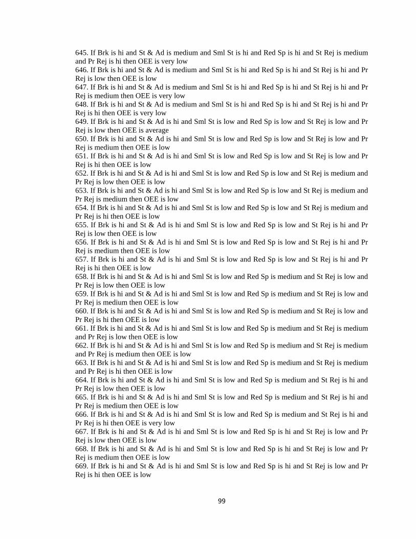
99
645. If Brk is hi and St & Ad is medium and Sml St is hi and Red Sp is hi and St Rej is medium
and Pr Rej is hi then OEE is very low
646. If Brk is hi and St & Ad is medium and Sml St is hi and Red Sp is hi and St Rej is hi and Pr
Rej is low then OEE is low
647. If Brk is hi and St & Ad is medium and Sml St is hi and Red Sp is hi and St Rej is hi and Pr
Rej is medium then OEE is very low
648. If Brk is hi and St & Ad is medium and Sml St is hi and Red Sp is hi and St Rej is hi and Pr
Rej is hi then OEE is very low
649. If Brk is hi and St & Ad is hi and Sml St is low and Red Sp is low and St Rej is low and Pr
Rej is low then OEE is average
650. If Brk is hi and St & Ad is hi and Sml St is low and Red Sp is low and St Rej is low and Pr
Rej is medium then OEE is low
651. If Brk is hi and St & Ad is hi and Sml St is low and Red Sp is low and St Rej is low and Pr
Rej is hi then OEE is low
652. If Brk is hi and St & Ad is hi and Sml St is low and Red Sp is low and St Rej is medium and
Pr Rej is low then OEE is low
653. If Brk is hi and St & Ad is hi and Sml St is low and Red Sp is low and St Rej is medium and
Pr Rej is medium then OEE is low
654. If Brk is hi and St & Ad is hi and Sml St is low and Red Sp is low and St Rej is medium and
Pr Rej is hi then OEE is low
655. If Brk is hi and St & Ad is hi and Sml St is low and Red Sp is low and St Rej is hi and Pr
Rej is low then OEE is low
656. If Brk is hi and St & Ad is hi and Sml St is low and Red Sp is low and St Rej is hi and Pr
Rej is medium then OEE is low
657. If Brk is hi and St & Ad is hi and Sml St is low and Red Sp is low and St Rej is hi and Pr
Rej is hi then OEE is low
658. If Brk is hi and St & Ad is hi and Sml St is low and Red Sp is medium and St Rej is low and
Pr Rej is low then OEE is low
659. If Brk is hi and St & Ad is hi and Sml St is low and Red Sp is medium and St Rej is low and
Pr Rej is medium then OEE is low
660. If Brk is hi and St & Ad is hi and Sml St is low and Red Sp is medium and St Rej is low and
Pr Rej is hi then OEE is low
661. If Brk is hi and St & Ad is hi and Sml St is low and Red Sp is medium and St Rej is medium
and Pr Rej is low then OEE is low
662. If Brk is hi and St & Ad is hi and Sml St is low and Red Sp is medium and St Rej is medium
and Pr Rej is medium then OEE is low
663. If Brk is hi and St & Ad is hi and Sml St is low and Red Sp is medium and St Rej is medium
and Pr Rej is hi then OEE is low
664. If Brk is hi and St & Ad is hi and Sml St is low and Red Sp is medium and St Rej is hi and
Pr Rej is low then OEE is low
665. If Brk is hi and St & Ad is hi and Sml St is low and Red Sp is medium and St Rej is hi and
Pr Rej is medium then OEE is low
666. If Brk is hi and St & Ad is hi and Sml St is low and Red Sp is medium and St Rej is hi and
Pr Rej is hi then OEE is very low
667. If Brk is hi and St & Ad is hi and Sml St is low and Red Sp is hi and St Rej is low and Pr
Rej is low then OEE is low
668. If Brk is hi and St & Ad is hi and Sml St is low and Red Sp is hi and St Rej is low and Pr
Rej is medium then OEE is low
669. If Brk is hi and St & Ad is hi and Sml St is low and Red Sp is hi and St Rej is low and Pr
Rej is hi then OEE is low

100
670. If Brk is hi and St & Ad is hi and Sml St is low and Red Sp is hi and St Rej is medium and
Pr Rej is low then OEE is low
671. If Brk is hi and St & Ad is hi and Sml St is low and Red Sp is hi and St Rej is medium and
Pr Rej is medium then OEE is low
672. If Brk is hi and St & Ad is hi and Sml St is low and Red Sp is hi and St Rej is medium and
Pr Rej is hi then OEE is very low
673. If Brk is hi and St & Ad is hi and Sml St is low and Red Sp is hi and St Rej is hi and Pr Rej
is low then OEE is low
674. If Brk is hi and St & Ad is hi and Sml St is low and Red Sp is hi and St Rej is hi and Pr Rej
is medium then OEE is very low
675. If Brk is hi and St & Ad is hi and Sml St is low and Red Sp is hi and St Rej is hi and Pr Rej
is hi then OEE is very low
676. If Brk is hi and St & Ad is hi and Sml St is medium and Red Sp is low and St Rej is low and
Pr Rej is low then OEE is low
677. If Brk is hi and St & Ad is hi and Sml St is medium and Red Sp is low and St Rej is low and
Pr Rej is medium then OEE is low
678. If Brk is hi and St & Ad is hi and Sml St is medium and Red Sp is low and St Rej is low and
Pr Rej is hi then OEE is low
679. If Brk is hi and St & Ad is hi and Sml St is medium and Red Sp is low and St Rej is medium
and Pr Rej is low then OEE is low
680. If Brk is hi and St & Ad is hi and Sml St is medium and Red Sp is low and St Rej is medium
and Pr Rej is medium then OEE is low
681. If Brk is hi and St & Ad is hi and Sml St is medium and Red Sp is low and St Rej is medium
and Pr Rej is hi then OEE is low
682. If Brk is hi and St & Ad is hi and Sml St is medium and Red Sp is low and St Rej is hi and
Pr Rej is low then OEE is low
683. If Brk is hi and St & Ad is hi and Sml St is medium and Red Sp is low and St Rej is hi and
Pr Rej is medium then OEE is low
684. If Brk is hi and St & Ad is hi and Sml St is medium and Red Sp is low and St Rej is hi and
Pr Rej is hi then OEE is very low
685. If Brk is hi and St & Ad is hi and Sml St is medium and Red Sp is medium and St Rej is low
and Pr Rej is low then OEE is low
686. If Brk is hi and St & Ad is hi and Sml St is medium and Red Sp is medium and St Rej is low
and Pr Rej is medium then OEE is low
687. If Brk is hi and St & Ad is hi and Sml St is medium and Red Sp is medium and St Rej is low
and Pr Rej is hi then OEE is low
688. If Brk is hi and St & Ad is hi and Sml St is medium and Red Sp is medium and St Rej is
medium and Pr Rej is low then OEE is low
689. If Brk is hi and St & Ad is hi and Sml St is medium and Red Sp is medium and St Rej is
medium and Pr Rej is medium then OEE is low
690. If Brk is hi and St & Ad is hi and Sml St is medium and Red Sp is medium and St Rej is
medium and Pr Rej is hi then OEE is very low
691. If Brk is hi and St & Ad is hi and Sml St is medium and Red Sp is medium and St Rej is hi
and Pr Rej is low then OEE is low
692. If Brk is hi and St & Ad is hi and Sml St is medium and Red Sp is medium and St Rej is hi
and Pr Rej is medium then OEE is very low
693. If Brk is hi and St & Ad is hi and Sml St is medium and Red Sp is medium and St Rej is hi
and Pr Rej is hi then OEE is very low
694. If Brk is hi and St & Ad is hi and Sml St is medium and Red Sp is hi and St Rej is low and
Pr Rej is low then OEE is low

101
695. If Brk is hi and St & Ad is hi and Sml St is medium and Red Sp is hi and St Rej is low and
Pr Rej is medium then OEE is low
696. If Brk is hi and St & Ad is hi and Sml St is medium and Red Sp is hi and St Rej is low and
Pr Rej is hi then OEE is very low
697. If Brk is hi and St & Ad is hi and Sml St is medium and Red Sp is hi and St Rej is medium
and Pr Rej is low then OEE is low
698. If Brk is hi and St & Ad is hi and Sml St is medium and Red Sp is hi and St Rej is medium
and Pr Rej is medium then OEE is very low
699. If Brk is hi and St & Ad is hi and Sml St is medium and Red Sp is hi and St Rej is medium
and Pr Rej is hi then OEE is very low
700. If Brk is hi and St & Ad is hi and Sml St is medium and Red Sp is hi and St Rej is hi and Pr
Rej is low then OEE is very low
701. If Brk is hi and St & Ad is hi and Sml St is medium and Red Sp is hi and St Rej is hi and Pr
Rej is medium then OEE is very low
702. If Brk is hi and St & Ad is hi and Sml St is medium and Red Sp is hi and St Rej is hi and Pr
Rej is hi then OEE is very low
703. If Brk is hi and St & Ad is hi and Sml St is hi and Red Sp is low and St Rej is low and Pr
Rej is low then OEE is low
704. If Brk is hi and St & Ad is hi and Sml St is hi and Red Sp is low and St Rej is low and Pr
Rej is medium then OEE is low
705. If Brk is hi and St & Ad is hi and Sml St is hi and Red Sp is low and St Rej is low and Pr
Rej is hi then OEE is low
706. If Brk is hi and St & Ad is hi and Sml St is hi and Red Sp is low and St Rej is medium and
Pr Rej is low then OEE is low
707. If Brk is hi and St & Ad is hi and Sml St is hi and Red Sp is low and St Rej is medium and
Pr Rej is medium then OEE is low
708. If Brk is hi and St & Ad is hi and Sml St is hi and Red Sp is low and St Rej is medium and
Pr Rej is hi then OEE is very low
709. If Brk is hi and St & Ad is hi and Sml St is hi and Red Sp is low and St Rej is hi and Pr Rej
is low then OEE is low
710. If Brk is hi and St & Ad is hi and Sml St is hi and Red Sp is low and St Rej is hi and Pr Rej
is medium then OEE is very low
711. If Brk is hi and St & Ad is hi and Sml St is hi and Red Sp is low and St Rej is hi and Pr Rej
is hi then OEE is very low
712. If Brk is hi and St & Ad is hi and Sml St is hi and Red Sp is medium and St Rej is low and
Pr Rej is low then OEE is low
713. If Brk is hi and St & Ad is hi and Sml St is hi and Red Sp is medium and St Rej is low and
Pr Rej is medium then OEE is low
714. If Brk is hi and St & Ad is hi and Sml St is hi and Red Sp is medium and St Rej is low and
Pr Rej is hi then OEE is very low
715. If Brk is hi and St & Ad is hi and Sml St is hi and Red Sp is medium and St Rej is medium
and Pr Rej is low then OEE is low
716. If Brk is hi and St & Ad is hi and Sml St is hi and Red Sp is medium and St Rej is medium
and Pr Rej is medium then OEE is very low
717. If Brk is hi and St & Ad is hi and Sml St is hi and Red Sp is medium and St Rej is medium
and Pr Rej is hi then OEE is very low
718. If Brk is hi and St & Ad is hi and Sml St is hi and Red Sp is medium and St Rej is hi and Pr
Rej is low then OEE is very low
719. If Brk is hi and St & Ad is hi and Sml St is hi and Red Sp is medium and St Rej is hi and Pr
Rej is medium then OEE is very low

102
720. If Brk is hi and St & Ad is hi and Sml St is hi and Red Sp is medium and St Rej is hi and Pr
Rej is hi then OEE is very low
721. If Brk is hi and St & Ad is hi and Sml St is hi and Red Sp is hi and St Rej is low and Pr Rej
is low then OEE is low
722. If Brk is hi and St & Ad is hi and Sml St is hi and Red Sp is hi and St Rej is low and Pr Rej
is medium then OEE is very low
723. If Brk is hi and St & Ad is hi and Sml St is hi and Red Sp is hi and St Rej is low and Pr Rej
is hi then OEE is very low
724. If Brk is hi and St & Ad is hi and Sml St is hi and Red Sp is hi and St Rej is medium and Pr
Rej is low then OEE is very low
725. If Brk is hi and St & Ad is hi and Sml St is hi and Red Sp is hi and St Rej is medium and Pr
Rej is medium then OEE is very low
726. If Brk is hi and St & Ad is hi and Sml St is hi and Red Sp is hi and St Rej is medium and Pr
Rej is hi then OEE is very low
727. If Brk is hi and St & Ad is hi and Sml St is hi and Red Sp is hi and St Rej is hi and Pr Rej is
low then OEE is very low
728. If Brk is hi and St & Ad is hi and Sml St is hi and Red Sp is hi and St Rej is hi and Pr Rej is
medium then OEE is very low
729. If Brk is hi and St & Ad is hi and Sml St is hi and Red Sp is hi and St Rej is hi and Pr Rej is
hi then OEE is very low
Section 2. OEE measurement using Sugeno Intelligent System 1, FIS if-then rules
1. If Brk is low and St & Ad is low and Sml St is low and Red Sp is low and St Rej is low and Pr
Rej is low then OEE is high
2. If Brk is medium and St & Ad is medium and Sml St is medium and Red Sp is medium and St
Rej is medium and Pr Rej is medium then OEE is medium
3. If Brk is hi and St & Ad is hi and Sml St is hi and Red Sp is hi and St Rej is hi and Pr Rej is hi
then OEE is low
Section 2. OEE measurement using Sugeno Intelligent System 2, FIS if-then rules
1. If Brk is low and St & Ad is low and Sml St is low and Red Sp is low and St Rej is low and Pr
Rej is low and Energy Consumption is low then OEE is high
2. If Brk is medium and St & Ad is medium and Sml St is medium and Red Sp is medium and St
Rej is medium and Pr Rej is medium and Energy Consumption is medium then OEE is medium
3. If Sml St is hi and Red Sp is hi and St Rej is hi and Pr Rej is hi and Energy Consumption is hi
then OEE is low
4. If Brk is hi or St & Ad is hi then OEE is low
As mentioned before, Sugeno FIS can be used in processes where a weight factor
can be allocated to inputs. In other words an equation can represent the contribution of
inputs into the system.

103
Section 3. OLE measurement using Mamdani FIS, IS 1 if-then rules
1. If OEE1 is low and OEE2 is low and OEE3 is low then OLE is very low
2. If OEE1 is low and OEE2 is low and OEE3 is medium then OLE is very low
3. If OEE1 is low and OEE2 is low and OEE3 is hi then OLE is low
4. If OEE1 is low and OEE2 is medium and OEE3 is low then OLE is low
5. If OEE1 is low and OEE2 is medium and OEE3 is medium then OLE is low
6. If OEE1 is low and OEE2 is medium and OEE3 is hi then OLE is average
7. If OEE1 is low and OEE2 is hi and OEE3 is low then OLE is average
8. If OEE1 is low and OEE2 is hi and OEE3 is medium then OLE is high
9. If OEE1 is low and OEE2 is hi and OEE3 is hi then OLE is high
10. If OEE1 is medium and OEE2 is low and OEE3 is low then OLE is very low
11. If OEE1 is medium and OEE2 is low and OEE3 is medium then OLE is low
12. If OEE1 is medium and OEE2 is low and OEE3 is hi then OLE is low
13. If OEE1 is medium and OEE2 is medium and OEE3 is low then OLE is low
14. If OEE1 is medium and OEE2 is medium and OEE3 is medium then OLE is average
15. If OEE1 is medium and OEE2 is medium and OEE3 is hi then OLE is high
16. If OEE1 is medium and OEE2 is hi and OEE3 is low then OLE is high
17. If OEE1 is medium and OEE2 is hi and OEE3 is medium then OLE is high
18. If OEE1 is medium and OEE2 is hi and OEE3 is hi then OLE is very high
19. If OEE1 is hi and OEE2 is low and OEE3 is low then OLE is low
20. If OEE1 is hi and OEE2 is low and OEE3 is medium then OLE is low
21. If OEE1 is hi and OEE2 is low and OEE3 is hi then OLE is average
22. If OEE1 is hi and OEE2 is medium and OEE3 is low then OLE is average
23. If OEE1 is hi and OEE2 is medium and OEE3 is medium then OLE is high
24. If OEE1 is hi and OEE2 is medium and OEE3 is hi then OLE is high
25. If OEE1 is hi and OEE2 is hi and OEE3 is low then OLE is high
26. If OEE1 is hi and OEE2 is hi and OEE3 is medium then OLE is very high
27. If OEE1 is hi and OEE2 is hi and OEE3 is hi then OLE is very high

104
Section 4. OLE measurement using Mamdani FIS, IS 2 if-then rules
1. If OEE1 is low and OEE2 is low and OEE3 is low then OLE is very low
2. If OEE1 is low and OEE2 is low and OEE3 is medium then OLE is very low
3. If OEE1 is low and OEE2 is low and OEE3 is hi then OLE is very low
4. If OEE1 is low and OEE2 is medium and OEE3 is low then OLE is very low
5. If OEE1 is low and OEE2 is medium and OEE3 is medium then OLE is low
6. If OEE1 is low and OEE2 is medium and OEE3 is hi then OLE is low
7. If OEE1 is low and OEE2 is hi and OEE3 is low then OLE is low
8. If OEE1 is low and OEE2 is hi and OEE3 is medium then OLE is average
9. If OEE1 is low and OEE2 is hi and OEE3 is hi then OLE is average
10. If OEE1 is medium and OEE2 is low and OEE3 is low then OLE is low
11. If OEE1 is medium and OEE2 is low and OEE3 is medium then OLE is low
12. If OEE1 is medium and OEE2 is low and OEE3 is hi then OLE is average
13. If OEE1 is medium and OEE2 is medium and OEE3 is low then OLE is average
14. If OEE1 is medium and OEE2 is medium and OEE3 is medium then OLE is average
15. If OEE1 is medium and OEE2 is medium and OEE3 is hi then OLE is average
16. If OEE1 is medium and OEE2 is hi and OEE3 is low then OLE is average
17. If OEE1 is medium and OEE2 is hi and OEE3 is medium then OLE is high
18. If OEE1 is medium and OEE2 is hi and OEE3 is hi then OLE is high
19. If OEE1 is hi and OEE2 is low and OEE3 is low then OLE is average
20. If OEE1 is hi and OEE2 is low and OEE3 is medium then OLE is average
21. If OEE1 is hi and OEE2 is low and OEE3 is hi then OLE is high
22. If OEE1 is hi and OEE2 is medium and OEE3 is low then OLE is high
23. If OEE1 is hi and OEE2 is medium and OEE3 is medium then OLE is high
24. If OEE1 is hi and OEE2 is medium and OEE3 is hi then OLE is very high
25. If OEE1 is hi and OEE2 is hi and OEE3 is low then OLE is very high
26. If OEE1 is hi and OEE2 is hi and OEE3 is medium then OLE is very high
27. If OEE1 is hi and OEE2 is hi and OEE3 is hi then OLE is very high

105
C. Mamdani Models Surface Plots
It is necessary to mention that surface plot of each Fuzzy Inference System represents the
results from various combinations of inputs and the sole output of the system. Note that
inputs and output of the Fuzzy Inference System are represented in the x, y and z axis
here.
Section 1. OEE Measurement using Mamdani Fuzzy Inference Systems

106

107
Section 2. OEE Measurement using Sugeno Fuzzy Inference Systems

108
Section 3. OLE Measurement using Mamdani Fuzzy Inference Systems

109
D. Mamdani and Sugeno Fuzzy Models if-then rules to measure OEE
Section 1. Mamdani FIS if-then rule to measure OEE

110
Section 2. Sugeno FIS if-then rule to measure OEE

111
Section 3. Mamdani FIS if-then rule to measure OLE

112
E. Artificial Neural Networks Matlab Code
Section 1. OLE Measurement using Artificial Neural Networks Matlab code
clear all clc % input P and output T P is the OEE of machines in a manufacturing
line. T % is the corresponding Overall Line Efficiency Please note that overall
line % efficiency above has calculated using Mamdani FIS.
P=[79.5000000000000,69.9200000000000,72.2200000000000,71.8700000000000,
69.4800000000000,67.8600000000000,70.0200000000000,66.5700000000000,78.
4900000000000,77.5400000000000,68.4100000000000,75.1700000000000,69.640
0000000000,79.1900000000000,72.1100000000000,79.1500000000000,65.870000
0000000,76.6200000000000,66.4400000000000,73.3700000000000,68.290000000
0000,69.2000000000000,67.6500000000000,69.1400000000000,66.640000000000
0,77.4700000000000,65.4300000000000,68.6900000000000,72.6000000000000,7
2.3100000000000,78.5900000000000,74.8300000000000,66.6200000000000,72.2
400000000000,73.4300000000000,69.0300000000000,75.8200000000000,68.9300
000000000,78.5500000000000,72.8700000000000,72.5100000000000,70.4700000
000000,68.8700000000000,69.8500000000000,67.9500000000000,77.1300000000
000,72.5700000000000,77.0200000000000,71.2100000000000,79.5300000000000
,65.6700000000000,76.0200000000000,65.1500000000000,70.7800000000000,65
.9300000000000,66.3700000000000,79.9600000000000,71.8000000000000,76.13
00000000000,69.5000000000000,68.9200000000000,77.9300000000000,75.39000
00000000,68.4000000000000,76.8200000000000,70.2100000000000,69.84000000
00000,76.3100000000000,73.2500000000000,69.6600000000000,76.66000000000
00,71.4800000000000,75.7900000000000,76.3900000000000,76.7600000000000,
75.9300000000000,78.2400000000000,70,66.8000000000000,78.1800000000000,
72.2300000000000,65.7700000000000,65.9400000000000,66.1100000000000,77.
4200000000000,72.6200000000000,75.4700000000000,72.1000000000000,65.720
0000000000,79.6600000000000,78.2400000000000,68.3400000000000,68.870000
0000000,65.3500000000000,70.3900000000000,66.8000000000000,78.460000000
0000;
75.4500000000000,71.4000000000000,76.1700000000000,70.6700000000000,78.
7700000000000,65.5300000000000,75.6800000000000,79.5900000000000,78.400
0000000000,76.1400000000000,75.4100000000000,77.8100000000000,68.330000
0000000,68.8800000000000,70.8000000000000,79.6600000000000,78.030000000
0000,68.5200000000000,68.8000000000000,67.3300000000000,79.290000000000
0,75.8900000000000,65.8500000000000,65.2700000000000,70.2400000000000,7
5.6000000000000,65.5500000000000,78.7400000000000,73.7600000000000,78.8
500000000000,77.6400000000000,65.8100000000000,75.8900000000000,67.5700
000000000,76.9800000000000,68.9500000000000,74.7500000000000,75.8600000
000000,73.8700000000000,65.4200000000000,66.0100000000000,76.2300000000
000,69.3500000000000,78.6900000000000,76.4600000000000,67.0200000000000
,79.2500000000000,78.2500000000000,74.8900000000000,78.4500000000000,77
.0200000000000,73.9500000000000,66.3600000000000,69.6400000000000,65.44
00000000000,74.4200000000000,69.3300000000000,67.7300000000000,75.68000
00000000,67.8900000000000,74.2000000000000,77.8500000000000,69.57000000
00000,72.6900000000000,67.7600000000000,66.5600000000000,65.68000000000
00,70.0900000000000,68.0900000000000,73.4400000000000,69.7500000000000,
66.1400000000000,71.2800000000000,69.9800000000000,73.8100000000000,71.
1500000000000,69.9000000000000,77.7500000000000,77.0700000000000,76,76.

113
0500000000000,69.1000000000000,72.1800000000000,72.0800000000000,78.150
0000000000,77.0800000000000,65.2000000000000,71.1300000000000,77.180000
0000000,73.8800000000000,74.2600000000000,73.0100000000000,79.260000000
0000,75.3000000000000,65.7700000000000,75.4600000000000,69.500000000000
0;
72.9500000000000,72.7400000000000,79.3700000000000,66.5300000000000,78.
6000000000000,77.4600000000000,76.9500000000000,74.8800000000000,77.250
0000000000,77.9100000000000,73.7500000000000,65.0700000000000,66.850000
0000000,67.1900000000000,72.5100000000000,79.7700000000000,73.040000000
0000,78.1500000000000,70.0400000000000,73.9700000000000,76.260000000000
0,69.3700000000000,78.5400000000000,75.7900000000000,77.3400000000000,7
2.1400000000000,73.6000000000000,73.5000000000000,70.5700000000000,66.5
100000000000,69.6900000000000,65.3900000000000,67.6500000000000,71.1800
000000000,77.4500000000000,74.1700000000000,68.4200000000000,67.5600000
000000,78.3000000000000,70.1800000000000,65.8900000000000,67.1400000000
000,69.6400000000000,74.9100000000000,68.0400000000000,69.6900000000000
,77.2200000000000,70.6000000000000,73.1600000000000,71.4900000000000,72
.7400000000000,78.0900000000000,77.5400000000000,76.0100000000000,78.63
00000000000,68.5600000000000,65.1200000000000,66.7400000000000,76.21000
00000000,78.7400000000000,66.7900000000000,79.1900000000000,70.48000000
00000,71.1800000000000,75.7600000000000,74.9200000000000,75.10000000000
00,68.8100000000000,78.1300000000000,70.9200000000000,68.8700000000000,
71.2100000000000,72.4300000000000,73.5200000000000,71.5500000000000,69.
3300000000000,67.6700000000000,65.8700000000000,79.7900000000000,72.970
0000000000,71.9000000000000,72.3600000000000,79.1900000000000,68.420000
0000000,69.6200000000000,74.8100000000000,66.9200000000000,78.820000000
0000,70.1500000000000,77.0100000000000,68.7400000000000,78.920000000000
0,69.4300000000000,65.5800000000000,70.2400000000000,69.7700000000000,7
2]; T(1,:)=[75.7600000000000,71.3720000000000,76.0200000000000,70.082000000
0000,76.8780000000000,68.3820000000000,74.8020000000000,76.044000000000
0,78.1880000000000,76.7740000000000,73.6780000000000,74.7340000000000,6
8.2960000000000,70.6040000000000,71.4040000000000,79.5800000000000,74.6
000000000000,72.0660000000000,68.5760000000000,69.8660000000000,76.4840
000000000,73.2480000000000,68.7480000000000,68.1480000000000,70.9400000
000000,75.2820000000000,67.1360000000000,75.6820000000000,72.8900000000
000,75.0740000000000,76.2400000000000,67.5300000000000,72.3880000000000
,69.2260000000000,76.3640000000000,70.0100000000000,73.6980000000000,72
.8140000000000,75.6920000000000,67.8620000000000,67.2860000000000,73.26
00000000000,69.3120000000000,76.1660000000000,73.0740000000000,69.57600
00000000,77.5080000000000,76.4740000000000,73.8080000000000,77.27400000
00000,73.8940000000000,75.1920000000000,68.3540000000000,71.14200000000
00,68.1760000000000,71.6380000000000,70.6140000000000,68.3460000000000,
75.8760000000000,70.3820000000000,71.6620000000000,78.1340000000000,70.
9160000000000,71.5300000000000,71.1720000000000,68.9620000000000,68.396
0000000000,71.0780000000000,71.1300000000000,72.1800000000000,70.956000
0000000,68.2220000000000,72.4120000000000,71.9700000000000,73.948000000
0000,71.7420000000000,71.1220000000000,73.8240000000000,75.560000000000
0,75.8300000000000,74.4560000000000,69.0860000000000,72.3340000000000,7
0.1540000000000,76.2980000000000,75.7340000000000,67.5980000000000,72.8
620000000000,73.4820000000000,75.6620000000000,73.9520000000000,73.2580
000000000,75.2160000000000,71.3660000000000,67.5880000000000,72.5900000
000000,71.7920000000000];
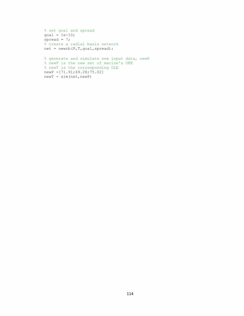
114
% set goal and spread goal = 1e-10; spread = 7; % create a radial basis network net = newrb(P,T,goal,spread);
% generate and simulate new input data, newP % newP is the new set of macine's OEE % newT is the corresponding OLE newP =[71.91;69.28;75.02] newT = sim(net,newP)

115
Section 2. Inverse Relationship of OLE and OEE, Artificial Neural Networks
Matlab code clear all clc % input P and output T P is the OEE of machines in a manufacturing
line. T % is the corresponding Overall Line Efficiency Please note that overall
line % efficiency above has calculated using Mamdani FIS.
P=[0.651900000000000,0.781600000000000,0.674800000000000,0.795000000000
000,0.699200000000000,0.722200000000000,0.718700000000000,0.69480000000
0000,0.678600000000000,0.700200000000000,0.665700000000000,0.7849000000
00000,0.775400000000000,0.684100000000000,0.751700000000000,0.696400000
000000,0.791900000000000,0.721100000000000,0.791500000000000,0.65870000
0000000,0.766200000000000,0.664400000000000,0.733700000000000,0.6829000
00000000,0.692000000000000,0.676500000000000,0.691400000000000,0.666400
000000000,0.774700000000000,0.654300000000000,0.686900000000000,0.72600
0000000000,0.723100000000000,0.785900000000000,0.748300000000000,0.6662
00000000000,0.722400000000000,0.734300000000000,0.690300000000000,0.758
200000000000,0.689300000000000,0.785500000000000,0.728700000000000,0.72
5100000000000,0.704700000000000,0.688700000000000,0.698500000000000,0.6
79500000000000,0.771300000000000,0.725700000000000,0.770200000000000,0.
712100000000000,0.795300000000000,0.656700000000000,0.760200000000000,0
.651500000000000,0.707800000000000,0.659300000000000,0.663700000000000,
0.799600000000000,0.718000000000000,0.761300000000000,0.695000000000000
,0.689200000000000,0.779300000000000,0.753900000000000,0.68400000000000
0,0.768200000000000,0.702100000000000,0.698400000000000,0.7631000000000
00,0.732500000000000,0.696600000000000,0.766600000000000,0.714800000000
000,0.757900000000000,0.763900000000000,0.767600000000000,0.75930000000
0000,0.782400000000000,0.700000000000000,0.668000000000000,0.7818000000
00000,0.722300000000000,0.657700000000000,0.659400000000000,0.661100000
000000,0.774200000000000,0.726200000000000,0.754700000000000,0.72100000
0000000,0.657200000000000,0.796600000000000,0.782400000000000,0.6834000
00000000,0.688700000000000,0.653500000000000,0.703900000000000,0.668000
000000000,0.784600000000000;0.719900000000000,0.719100000000000,0.67830
0000000000,0.754500000000000,0.714000000000000,0.761700000000000,0.7067
00000000000,0.787700000000000,0.655300000000000,0.756800000000000,0.795
900000000000,0.784000000000000,0.761400000000000,0.754100000000000,0.77
8100000000000,0.683300000000000,0.688800000000000,0.708000000000000,0.7
96600000000000,0.780300000000000,0.685200000000000,0.688000000000000,0.
673300000000000,0.792900000000000,0.758900000000000,0.658500000000000,0
.652700000000000,0.702400000000000,0.756000000000000,0.655500000000000,
0.787400000000000,0.737600000000000,0.788500000000000,0.776400000000000
,0.658100000000000,0.758900000000000,0.675700000000000,0.76980000000000
0,0.689500000000000,0.747500000000000,0.758600000000000,0.7387000000000
00,0.654200000000000,0.660100000000000,0.762300000000000,0.693500000000
000,0.786900000000000,0.764600000000000,0.670200000000000,0.79250000000
0000,0.782500000000000,0.748900000000000,0.784500000000000,0.7702000000
00000,0.739500000000000,0.663600000000000,0.696400000000000,0.654400000
000000,0.744200000000000,0.693300000000000,0.677300000000000,0.75680000
0000000,0.678900000000000,0.742000000000000,0.778500000000000,0.6957000
00000000,0.726900000000000,0.677600000000000,0.665600000000000,0.656800
000000000,0.700900000000000,0.680900000000000,0.734400000000000,0.69750

116
0000000000,0.661400000000000,0.712800000000000,0.699800000000000,0.7381
00000000000,0.711500000000000,0.699000000000000,0.777500000000000,0.770
700000000000,0.760000000000000,0.760500000000000,0.691000000000000,0.72
1800000000000,0.720800000000000,0.781500000000000,0.770800000000000,0.6
52000000000000,0.711300000000000,0.771800000000000,0.738800000000000,0.
742600000000000,0.730100000000000,0.792600000000000,0.753000000000000,0
.657700000000000,0.754600000000000,0.695000000000000;0.732500000000000,
0.791000000000000,0.690400000000000,0.729500000000000,0.727400000000000
,0.793700000000000,0.665300000000000,0.786000000000000,0.77460000000000
0,0.769500000000000,0.748800000000000,0.772500000000000,0.7791000000000
00,0.737500000000000,0.650700000000000,0.668500000000000,0.671900000000
000,0.725100000000000,0.797700000000000,0.730400000000000,0.78150000000
0000,0.700400000000000,0.739700000000000,0.762600000000000,0.6937000000
00000,0.785400000000000,0.757900000000000,0.773400000000000,0.721400000
000000,0.736000000000000,0.735000000000000,0.705700000000000,0.66510000
0000000,0.696900000000000,0.653900000000000,0.676500000000000,0.7118000
00000000,0.774500000000000,0.741700000000000,0.684200000000000,0.675600
000000000,0.783000000000000,0.701800000000000,0.658900000000000,0.67140
0000000000,0.696400000000000,0.749100000000000,0.680400000000000,0.6969
00000000000,0.772200000000000,0.706000000000000,0.731600000000000,0.714
900000000000,0.727400000000000,0.780900000000000,0.775400000000000,0.76
0100000000000,0.786300000000000,0.685600000000000,0.651200000000000,0.6
67400000000000,0.762100000000000,0.787400000000000,0.667900000000000,0.
791900000000000,0.704800000000000,0.711800000000000,0.757600000000000,0
.749200000000000,0.751000000000000,0.688100000000000,0.781300000000000,
0.709200000000000,0.688700000000000,0.712100000000000,0.724300000000000
,0.735200000000000,0.715500000000000,0.693300000000000,0.67670000000000
0,0.658700000000000,0.797900000000000,0.729700000000000,0.7190000000000
00,0.723600000000000,0.791900000000000,0.684200000000000,0.696200000000
000,0.748100000000000,0.669200000000000,0.788200000000000,0.70150000000
0000,0.770100000000000,0.687400000000000,0.789200000000000,0.6943000000
00000,0.655800000000000,0.702400000000000,0.697700000000000,0.720000000
000000;]; T=[0.708820000000000,0.745980000000000,0.680020000000000,0.757600000000
000,0.713720000000000,0.760200000000000,0.700820000000000,0.76878000000
0000,0.683820000000000,0.748020000000000,0.760440000000000,0.7818800000
00000,0.767740000000000,0.736780000000000,0.747340000000000,0.682960000
000000,0.706040000000000,0.714040000000000,0.795800000000000,0.74600000
0000000,0.720660000000000,0.685760000000000,0.698660000000000,0.7648400
00000000,0.732480000000000,0.687480000000000,0.681480000000000,0.709400
000000000,0.752820000000000,0.671360000000000,0.756820000000000,0.72890
0000000000,0.750740000000000,0.762400000000000,0.675300000000000,0.7238
80000000000,0.692260000000000,0.763640000000000,0.700100000000000,0.736
980000000000,0.728140000000000,0.756920000000000,0.678620000000000,0.67
2860000000000,0.732600000000000,0.693120000000000,0.761660000000000,0.7
30740000000000,0.695760000000000,0.775080000000000,0.764740000000000,0.
738080000000000,0.772740000000000,0.738940000000000,0.751920000000000,0
.683540000000000,0.711420000000000,0.681760000000000,0.716380000000000,
0.706140000000000,0.683460000000000,0.758760000000000,0.703820000000000
,0.716620000000000,0.781340000000000,0.709160000000000,0.71530000000000
0,0.711720000000000,0.689620000000000,0.683960000000000,0.7107800000000
00,0.711300000000000,0.721800000000000,0.709560000000000,0.682220000000
000,0.724120000000000,0.719700000000000,0.739480000000000,0.71742000000
0000,0.711220000000000,0.738240000000000,0.755600000000000,0.7583000000
00000,0.744560000000000,0.690860000000000,0.723340000000000,0.701540000
000000,0.762980000000000,0.757340000000000,0.675980000000000,0.72862000
0000000,0.734820000000000,0.756620000000000,0.739520000000000,0.7325800

117
00000000,0.752160000000000,0.713660000000000,0.675880000000000,0.725900
000000000,0.717920000000000;];
% set goal and spread %CREATING DUMMIES
T(2,:)=(((P(1,:)+P(2,:))/2)-1).^2; T(3,:)=(((P(2,:)+P(3,:))/2)-1).^2;
% set goal and spread
goal = 1e-10; spread = 7;
% create a radial basis network net = newrb(T,P,goal,spread);
% generate and simulate new input data, newP % newP is the new set of machine’s OEE % newT is the corresponding OLE newT =[0.79; 0.05; 0.04] newP = sim(net,newT)

118
F. Artificial Neural Network Performance plot
Section 1. Performance Plot of Artificial Neural Networks to Measure OLE
NEWRB, neurons = 0, MSE = 9.23127
NEWRB, neurons = 25, MSE = 0.0204861
NEWRB, neurons = 50, MSE = 0.00163035
NEWRB, neurons = 75, MSE = 5.80586e-005
newP =
71.9100
69.2800
75.0200
newT =
70.9710
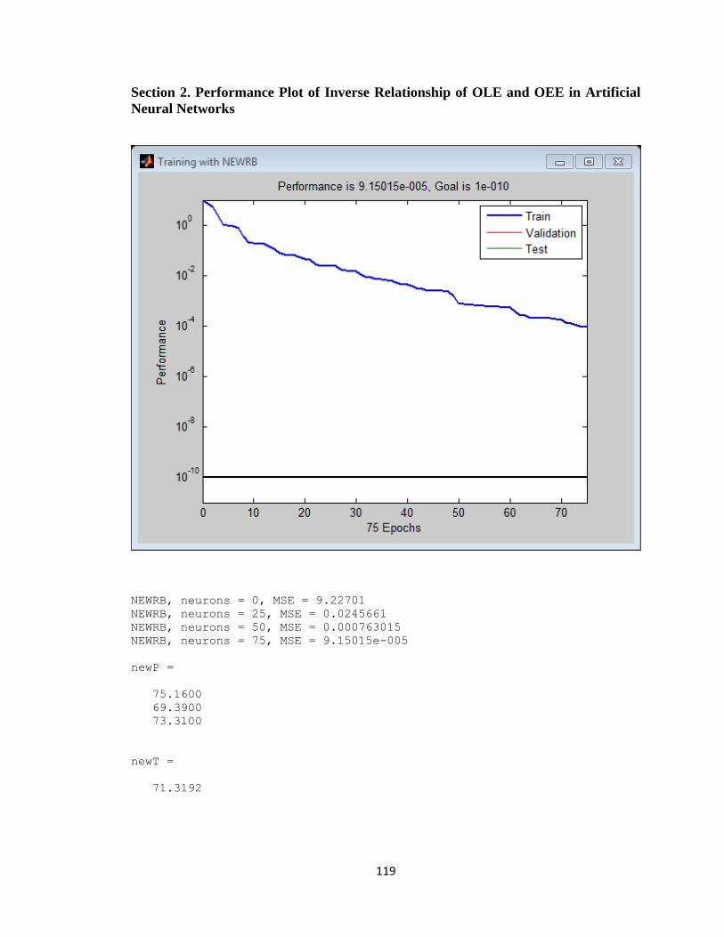
119
Section 2. Performance Plot of Inverse Relationship of OLE and OEE in Artificial
Neural Networks
NEWRB, neurons = 0, MSE = 9.22701
NEWRB, neurons = 25, MSE = 0.0245661
NEWRB, neurons = 50, MSE = 0.000763015
NEWRB, neurons = 75, MSE = 9.15015e-005
newP =
75.1600
69.3900
73.3100
newT =
71.3192