Quantization - ivp.ee.cuhk.edu.hk
34
1 ELEG5502 Video Coding Technology Quantization • Quantization discretizes the continuous-amplitude samples to one of L discrete-amplitude levels represented by a binary codeword of R bits. • Consider an input x with amplitudes in the range (1) and a uniform quantizer with x min = − x max as in Fig. 3.21. In this case, the quantizer stepsize ∆ has equal distance between the decision levels and the reconstruction levels where L is the number of quantization levels. • The stepsize is (2) where ) , ( max min x x x ∈ , ...., 2, , 1 , L k x k = , 1 ...., 2, , 1 , − = L k y k 1 2 2 max − = ∆ R x . log 2 L R =
Transcript of Quantization - ivp.ee.cuhk.edu.hk
1 ELEG5502 Video Coding Technology
Quantization
• Quantization discretizes the continuous-amplitude samples to one of L discrete-amplitude levels represented by a binary codeword of R bits.
• Consider an input x with amplitudes in the range
(1)
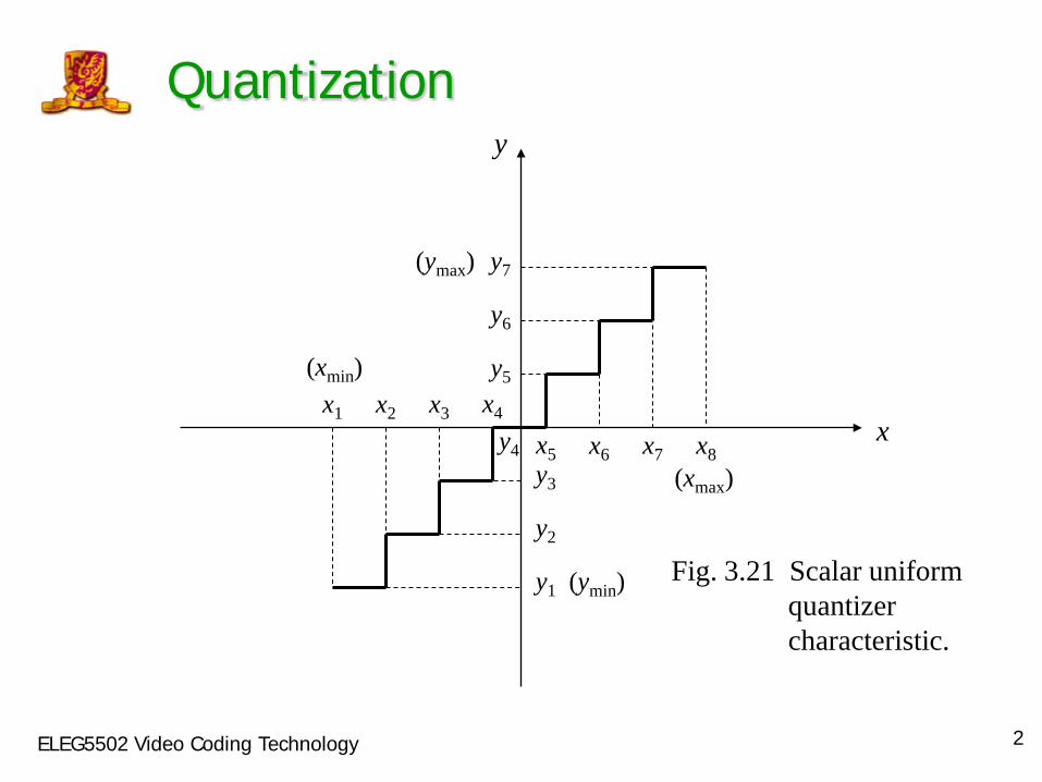
and a uniform quantizer with xmin = − xmax as in Fig. 3.21. In this case, the quantizer stepsize ∆ has equal distance between the decision levels and the reconstruction levels where L is the number of quantization levels.
• The stepsize is
(2)
where
) ,( maxmin xxx∈
, ...., 2, ,1 , Lkxk =, 1 ...., 2, ,1 , −= Lkyk
122 max
−=∆ R
x
. log2 LR =
2 ELEG5502 Video Coding Technology
Quantization
Fig. 3.21 Scalar uniform quantizer characteristic.
x
y
x1 x2 x3 x4 x5 x6 x7 x8 y4
y5
(xmax)
(xmin)
y1
y2
y3
y6
y7
(ymin)
(ymax)
3 ELEG5502 Video Coding Technology
Quantization
• The decision and reconstruction levels are given by
(3)
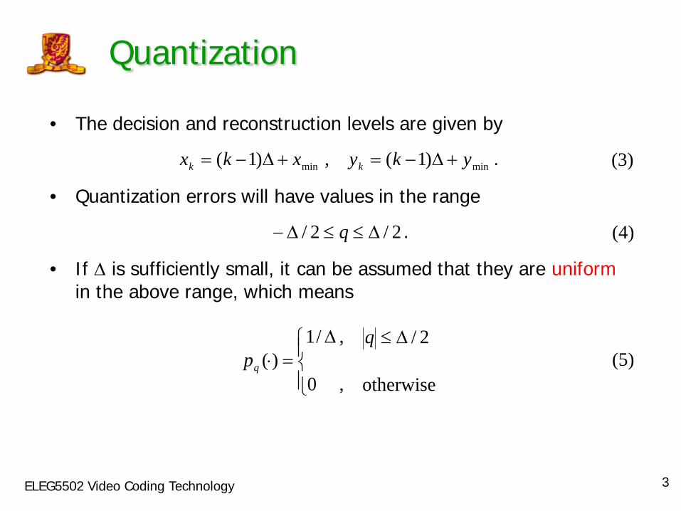
• Quantization errors will have values in the range
(4)
• If ∆ is sufficiently small, it can be assumed that they are uniform in the above range, which means
(5)
. 2/2/ ∆≤≤∆− q
otherwise
2/
,
,
0
/1)(
∆≤
∆
=⋅q
pq
. )1(,)1( minmin ykyxkx kk +∆−=+∆−=
4 ELEG5502 Video Coding Technology
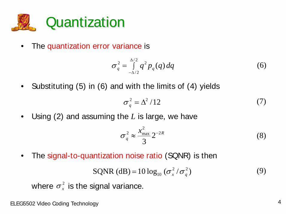
Quantization • The quantization error variance is
(6)
• Substituting (5) in (6) and with the limits of (4) yields
(7)
• Using (2) and assuming the L is large, we have
(8)
• The signal-to-quantization noise ratio (SQNR) is then
(9)
where is the signal variance.
∫∆
∆−=
2/
2/
22 )( dqqpq qqσ
12/22 ∆=qσ
Rq
x 22max2 23
−≈σ
)/( log 10(dB) SQNR 2210 qx σσ=
2xσ
5 ELEG5502 Video Coding Technology
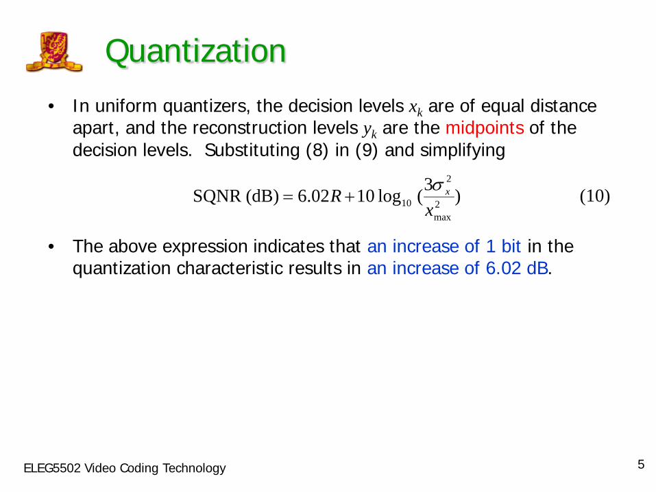
Quantization • In uniform quantizers, the decision levels xk are of equal distance
apart, and the reconstruction levels yk are the midpoints of the decision levels. Substituting (8) in (9) and simplifying
(10)
• The above expression indicates that an increase of 1 bit in the quantization characteristic results in an increase of 6.02 dB.
)3( log 1002.6(dB) SQNR 2
max
2
10 xR xσ+=
6 ELEG5502 Video Coding Technology
Quantization
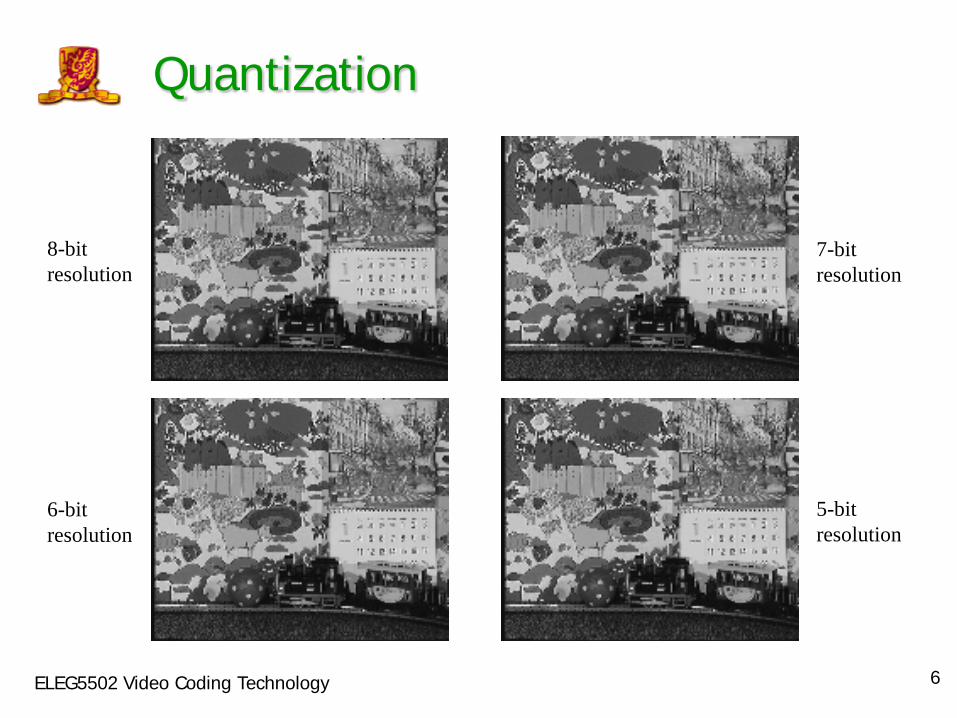
7-bit resolution
5-bit resolution
6-bit resolution
8-bit resolution
7 ELEG5502 Video Coding Technology
Quantization
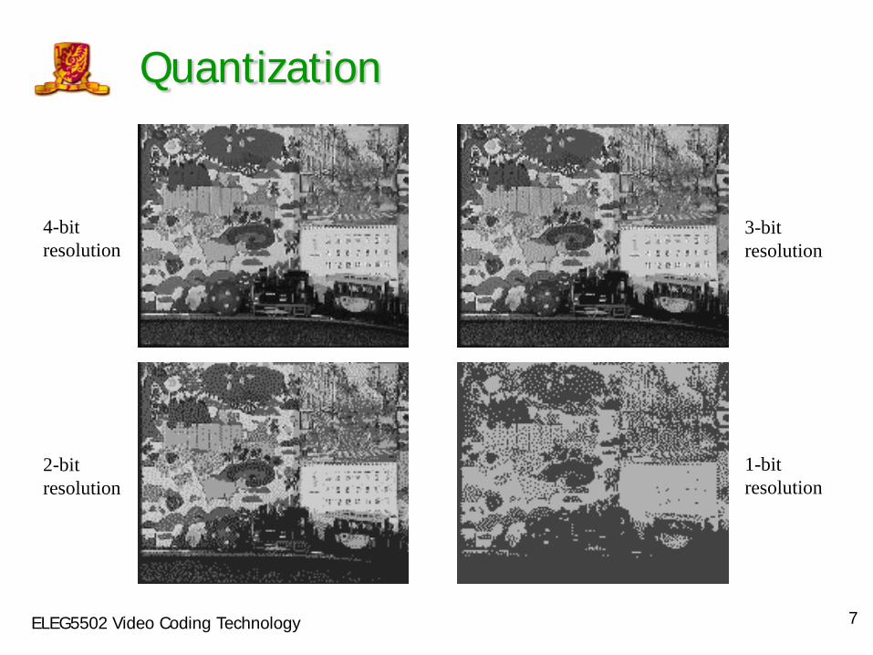
1-bit resolution
2-bit resolution
3-bit resolution
4-bit resolution
8 ELEG5502 Video Coding Technology
Non-uniform Quantization
Non-uniform Quantization
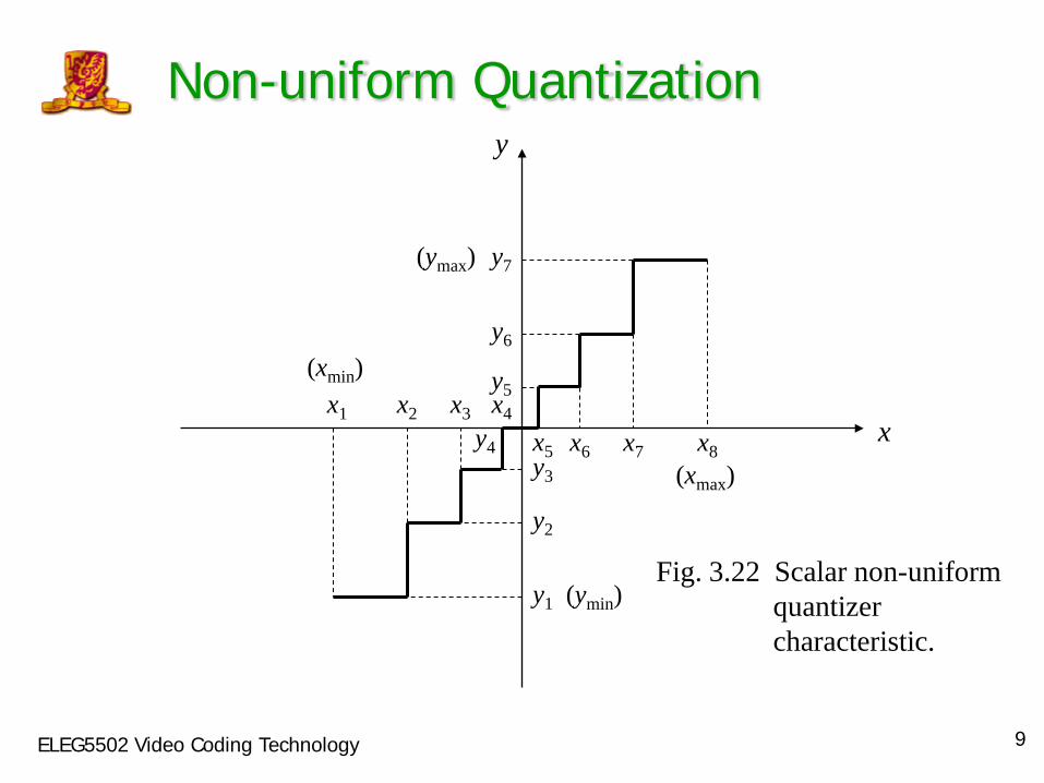
• Uniform quantization assumes uniform pdf within the quantizer step sizes. However, natural video signals generally do not obey uniform distribution.
• It has been shown that the frame difference signals assume a Laplacian pdf, which means that low amplitude signals predominate. Therefore, a quantizer with smaller stepsizes for low amplitude range and larger ones for high amplitude range will reduce the quantization noise.
• A non-uniform quantizer can be designed according to the pdf of the signals it quantizes. Such quantizers are called pdf-optimized non-uniform quantizers.
9 ELEG5502 Video Coding Technology
Non-uniform Quantization
Fig. 3.22 Scalar non-uniform quantizer characteristic.
x2 x3 x4 x5 x6 x7
y2
y3 y4
y5
y6
x8 (xmax)
y
x1 (xmin)
y1 (ymin)
y7 (ymax)
x
10 ELEG5502 Video Coding Technology
Non-uniform Quantization
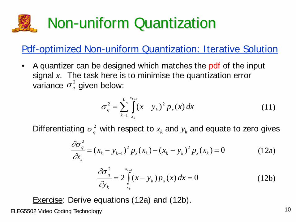
Pdf-optimized Non-uniform Quantization: Iterative Solution
• A quantizer can be designed which matches the pdf of the input signal x. The task here is to minimise the quantization error variance given below:
(11)
Differentiating with respect to xk and yk and equate to zero gives
(12a)
(12b)
Exercise: Derive equations (12a) and (12b).
2qσ
∑ ∫=
+
−=L
k
x
xxkq
k
k
dxxpyx1
221
)()(σ
0)()()()( 221
2
=−−−= − kxkkkxkkk
q xpyxxpyxx∂
∂σ
0)()(212
=−= ∫+k
k
x
xxk
k
q dxxpyxy∂
∂σ
2qσ
11 ELEG5502 Video Coding Technology
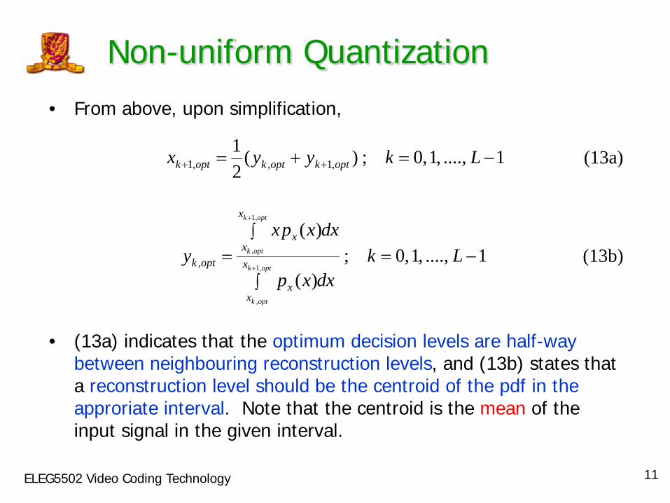
Non-uniform Quantization • From above, upon simplification,
(13a)
(13b)
• (13a) indicates that the optimum decision levels are half-way
between neighbouring reconstruction levels, and (13b) states that a reconstruction level should be the centroid of the pdf in the approriate interval. Note that the centroid is the mean of the input signal in the given interval.
1 ...., ,1 ,0;)(21
,1,,1 −=+= ++ Lkyyx optkoptkoptk
1 ...., ,1 ,0;)(
)(
,1
,
,1
,
, −==∫
∫
+
+
Lkdxxp
dxxpxy
optk
optk
optk
optk
x
xx
x
xx
optk
12 ELEG5502 Video Coding Technology
Non-uniform Quantization
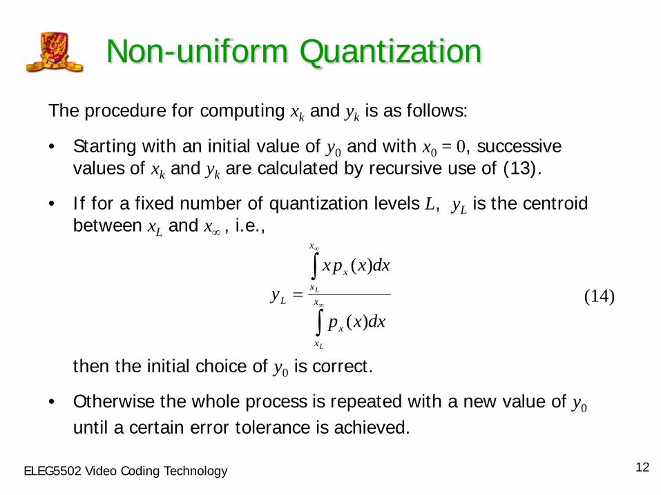
The procedure for computing xk and yk is as follows:
• Starting with an initial value of y0 and with x0 = 0, successive values of xk and yk are calculated by recursive use of (13).
• If for a fixed number of quantization levels L, yL is the centroid between xL and x∞ , i.e.,
(14)
then the initial choice of y0 is correct.
• Otherwise the whole process is repeated with a new value of y0 until a certain error tolerance is achieved.
∫
∫∞
∞
= x
xx
x
xx
L
L
L
dxxp
dxxpxy
)(
)(
13 ELEG5502 Video Coding Technology
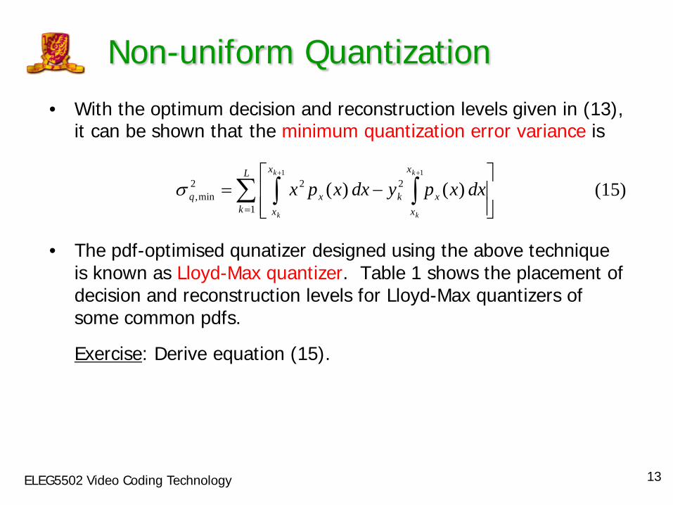
Non-uniform Quantization • With the optimum decision and reconstruction levels given in (13),
it can be shown that the minimum quantization error variance is
(15)
• The pdf-optimised qunatizer designed using the above technique
is known as Lloyd-Max quantizer. Table 1 shows the placement of decision and reconstruction levels for Lloyd-Max quantizers of some common pdfs.
Exercise: Derive equation (15).
∑ ∫ ∫
=
−=
+ +L
k
x
x
x
xxkxq
k
k
k
k
dxxpydxxpx1
222min,
1 1
)()(σ
14 ELEG5502 Video Coding Technology
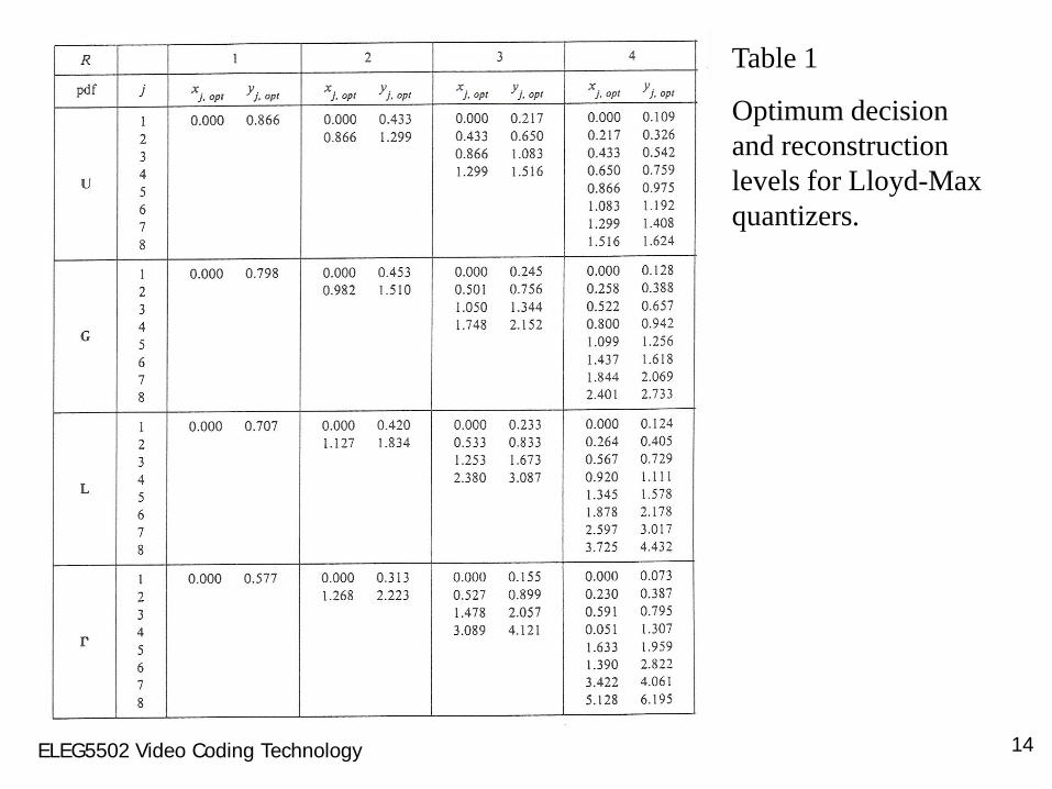
Table 1
Optimum decision and reconstruction levels for Lloyd-Max quantizers.
15 ELEG5502 Video Coding Technology
Entropy Coding
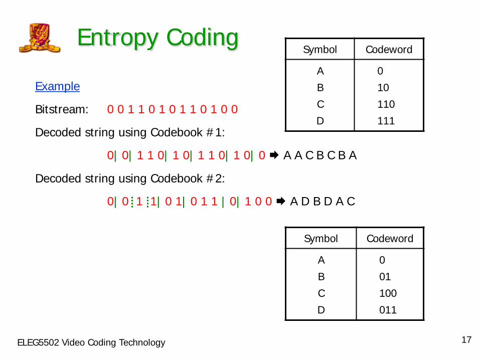
• Entropy coding is a lossless coding technique whereby a possible symbol from a finite alphabet source is represented by binary bits, called a codeword.
• A symbol may correspond to one or several original or quantized pixel values or model parameters.
• A codeword may be of fixed-length or of variable-length. The codewords for all possible symbols form a codebook or code table.
• For a code to be useful, it should have the following properties: 1. it should be uniquely decodable;
2. it should be instantaneously decodable.
16 ELEG5502 Video Coding Technology
Entropy Coding
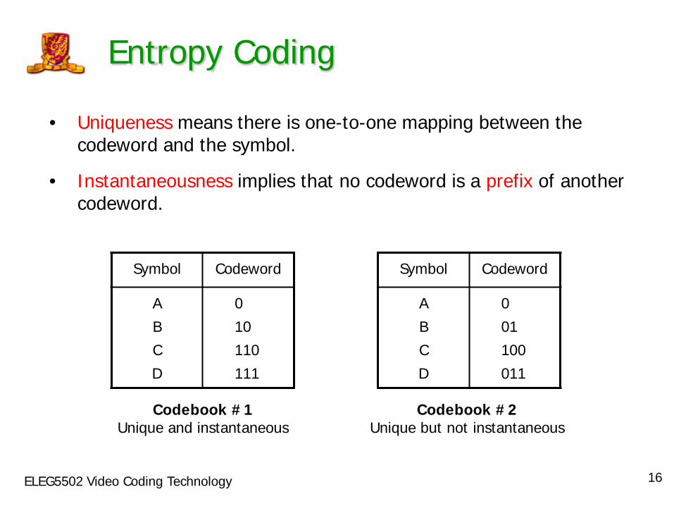
• Uniqueness means there is one-to-one mapping between the codeword and the symbol.
• Instantaneousness implies that no codeword is a prefix of another codeword.
Symbol Codeword
A
B
C
D
0
10
110
111
Symbol Codeword
A
B
C
D
0
01
100
011
Codebook #1 Unique and instantaneous
Codebook #2 Unique but not instantaneous
17 ELEG5502 Video Coding Technology
Entropy Coding
Example
Bitstream: 0 0 1 1 0 1 0 1 1 0 1 0 0
Decoded string using Codebook #1:
0| 0| 1 1 0| 1 0| 1 1 0| 1 0| 0 A A C B C B A
Decoded string using Codebook #2:
0| 0 1 1| 0 1| 0 1 1 | 0| 1 0 0 A D B D A C
Symbol Codeword
A
B
C
D
0
10
110
111
Symbol Codeword
A
B
C
D
0
01
100
011
18 ELEG5502 Video Coding Technology
Runlength Coding
Runlength Coding
• Runlength coding (RLC) codes a binary sequence as length of runs of 0s, i.e., the number of 0s between successive 1s. It is useful whenever large runs of 0s are expected as in printed documents, graphics, weather maps, etc., where the probability of a 0, p, is close to unity.
• Suppose each run is coded with a fixed-length code of m bits resulting in a maximum length of M where . If the successive 0s occur independently, then the probability distribution of the runlengths turns out to be the geometric distribution.
12 −= mM
19 ELEG5502 Video Coding Technology
Runlength Coding
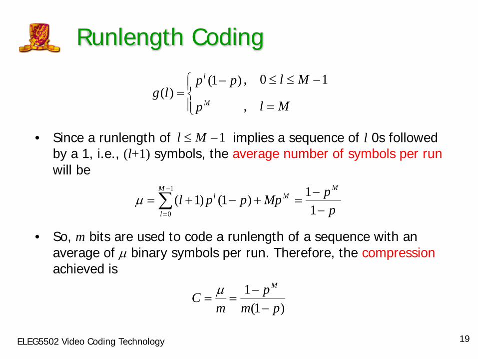
• Since a runlength of implies a sequence of l 0s followed by a 1, i.e., (l+1) symbols, the average number of symbols per run will be
• So, m bits are used to code a runlength of a sequence with an average of µ binary symbols per run. Therefore, the compression achieved is
Ml
Ml
p
pplg
M
l
=
−≤≤
−
=,
10,)1()(
1−≤ Ml
∑−
= −−
=+−+=1
0 11)1()1(
M
l
MMl
ppMppplµ
)1(1
pmp
mC
M
−−
==µ
20 ELEG5502 Video Coding Technology
Runlength Coding
• For example, for p = 0.9 and M = 15, we obtain m = 4, µ = 7.94, and C = 1.985. The average bit rate is R = m / µ = 0.516 bits per symbol and the code efficiency, defined as H / R , is 0.469 / 0.516 = 91% . For a given value of p, the optimum value of M can be determined to give the highest efficiency.
• RLC can also be applied to code multi-level samples as shown by the example on the next slide.
• RLC efficiency can be further improved by using a variable length coding technique such as Huffman coding to code the combinations of zero-runlength and amplitude.
21 ELEG5502 Video Coding Technology
Runlength Coding
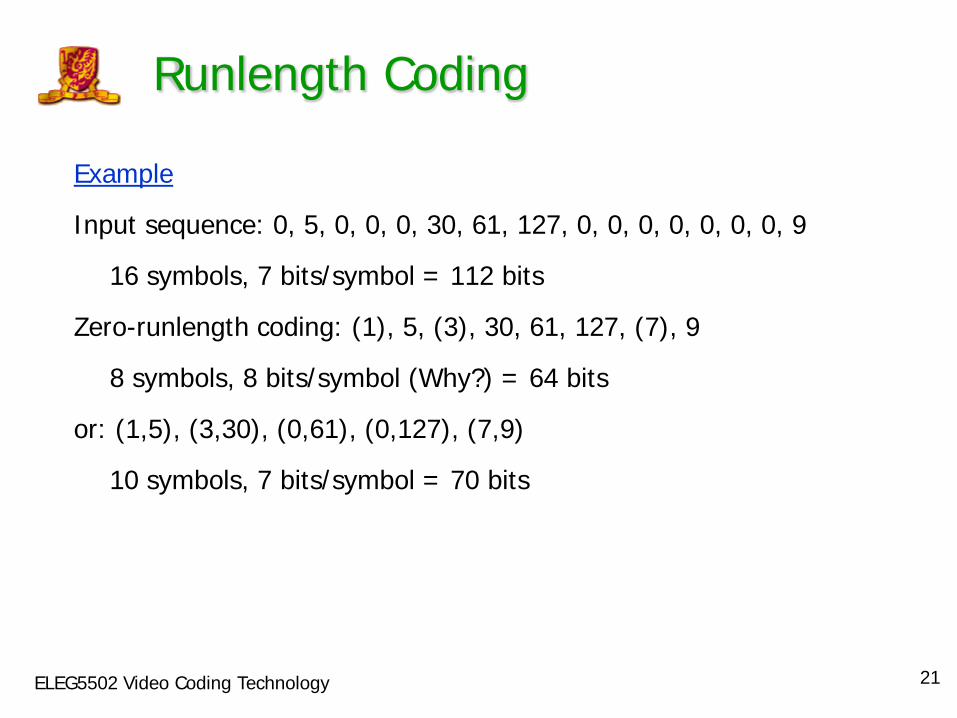
Example
Input sequence: 0, 5, 0, 0, 0, 30, 61, 127, 0, 0, 0, 0, 0, 0, 0, 9
16 symbols, 7 bits/symbol = 112 bits
Zero-runlength coding: (1), 5, (3), 30, 61, 127, (7), 9
8 symbols, 8 bits/symbol (Why?) = 64 bits
or: (1,5), (3,30), (0,61), (0,127), (7,9)
10 symbols, 7 bits/symbol = 70 bits
22 ELEG5502 Video Coding Technology
Huffman Coding Huffman Coding
• For non-uniformly distributed symbols, their entropy, H will be less than the average bit rate of the original data.
• Huffman codes are designed according to the probabilities of the symbols so that the average bit rate R defined as
where Li is the symbol codelength, pi the symbol probability and M the number of symbols, is equal to the entropy H.
• This gives a variable-length code for each block, where highly probable blocks (or symbols) are represented by short-length codes, and vice versa.
• Huffman codes are uniquely and instantaneously decodable.
∑=
=M
iii pLR
1
23 ELEG5502 Video Coding Technology
Huffman Coding
1. Arrange the symbols probabilities in a descending order and consider them as leaf nodes of a tree.
2. While there is more than one node: – Merge the two nodes with the smallest probability to form a new
node whose probability is the sum of the two merged nodes. – Arbitrarily assign 1 and 0 to each pair of branches merging into a
node.
3. Read sequentially from the root node to the leaf node where the symbol is located. The bit at the leaf node is the last bit of the codeword.
The Huffman codebook for a set of probabilities is generated by the following steps:
24 ELEG5502 Video Coding Technology
Huffman Coding
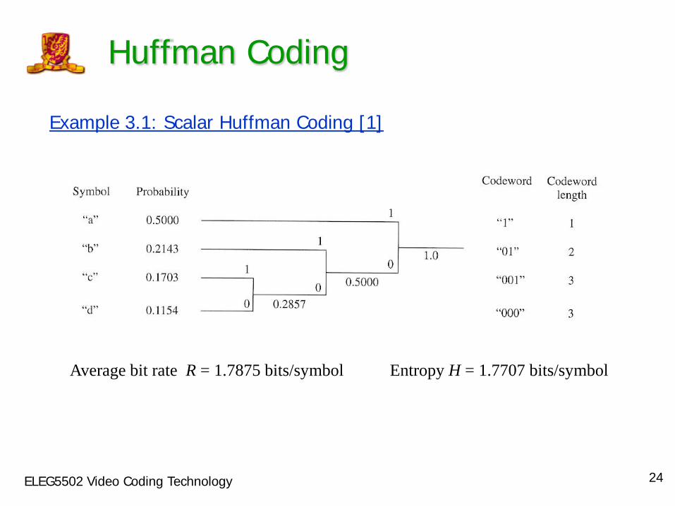
Example 3.1: Scalar Huffman Coding [1]
Average bit rate R = 1.7875 bits/symbol Entropy H = 1.7707 bits/symbol
25 ELEG5502 Video Coding Technology
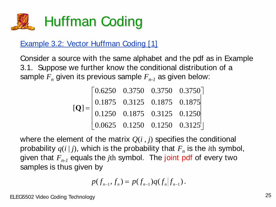
Huffman Coding Example 3.2: Vector Huffman Coding [1]
Consider a source with the same alphabet and the pdf as in Example 3.1. Suppose we further know the conditional distribution of a sample Fn given its previous sample Fn-1 as given below:
where the element of the matrix Q(i , j) specifies the conditional probability q(i | j), which is the probability that Fn is the ith symbol, given that Fn-1 equals the jth symbol. The joint pdf of every two samples is thus given by
=
3125.01250.01250.00625.01250.03125.01875.01250.01875.01875.03125.01875.03750.03750.03750.06250.0
][Q
. )()(),( 111 −−− = nnnnn ffqfpffp
26 ELEG5502 Video Coding Technology
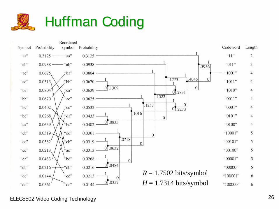
Huffman Coding
R = 1.7502 bits/symbol H = 1.7314 bits/symbol
27 ELEG5502 Video Coding Technology
Huffman Coding
• Encoding and decoding is done simply by table look-up. Note that the codewords are uniquely and instantaneously decodable. This is because no codeword can be a prefix of any longer-length codeword. Since the codewords have variable lengths, a buffer is needed to smooth the data flow when transmitted over a constant-rate channel.
• Huffman coding is ideal for signals with non-uniform probability distributions. Therefore, it may not be efficient in coding raw image data. However, it is useful for coding the quantized output of predictive or transform coder and also for graphics and facsimile images.
28 ELEG5502 Video Coding Technology
Arithmetic Coding
• Arithmetic coding (AC) is a coding technique that approaches the entropy limit.
• In AC, a message is represented by an interval of real numbers between 0 and 1.
• As the message becomes longer, the interval needed to represent it becomes smaller, and the number of bits needed to specify that interval grows.
• Successive symbols of the message reduce the size of the interval in accordance with the symbol probabilities generated by the model.
• The more likely symbols reduce the range by a smaller amount than the less likely symbols do and hence introduce fewer bits to the message.
29 ELEG5502 Video Coding Technology
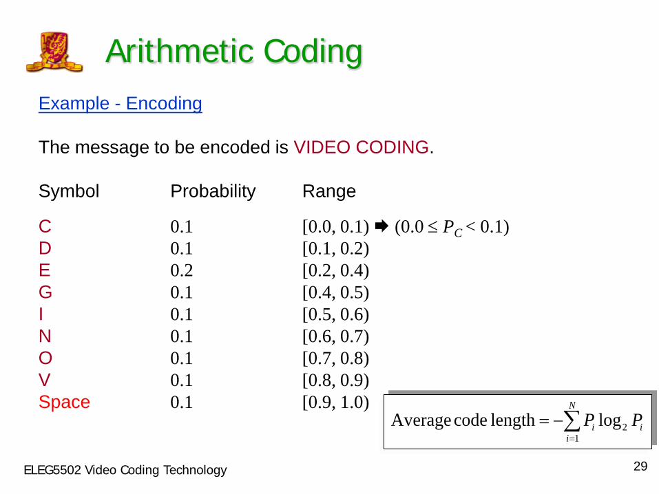
Arithmetic Coding Example - Encoding The message to be encoded is VIDEO CODING. Symbol Probability Range
C 0.1 [0.0, 0.1) (0.0 ≤ PC < 0.1) D 0.1 [0.1, 0.2) E 0.2 [0.2, 0.4) G 0.1 [0.4, 0.5) I 0.1 [0.5, 0.6) N 0.1 [0.6, 0.7) O 0.1 [0.7, 0.8) V 0.1 [0.8, 0.9) Space 0.1 [0.9, 1.0)
∑=
−=N
iii PP
12loglength code Average
30 ELEG5502 Video Coding Technology
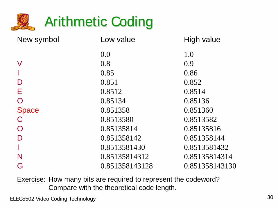
Arithmetic Coding New symbol Low value High value
0.0 1.0 V 0.8 0.9 I 0.85 0.86 D 0.851 0.852 E 0.8512 0.8514 O 0.85134 0.85136 Space 0.851358 0.851360 C 0.8513580 0.8513582 O 0.85135814 0.85135816 D 0.851358142 0.851358144 I 0.8513581430 0.8513581432 N 0.85135814312 0.85135814314 G 0.851358143128 0.851358143130
Exercise: How many bits are required to represent the codeword? Compare with the theoretical code length.
31 ELEG5502 Video Coding Technology
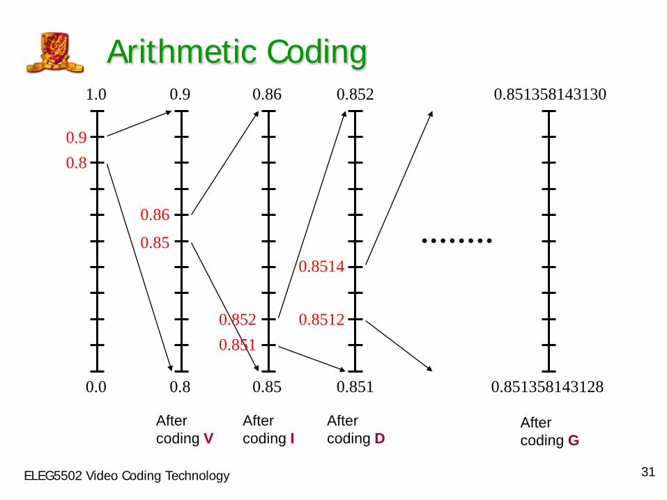
Arithmetic Coding
1.0
0.0
0.8 0.9
0.9
0.8
0.85
0.86
0.86
0.85
0.852
0.851
0.851 0.852 0.8512
0.8514 • • • • • • • •
0.851358143130
0.851358143128
After coding V
After coding I
After coding D
After coding G
32 ELEG5502 Video Coding Technology
Arithmetic Coding
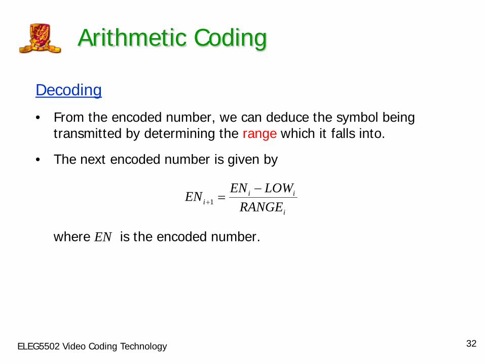
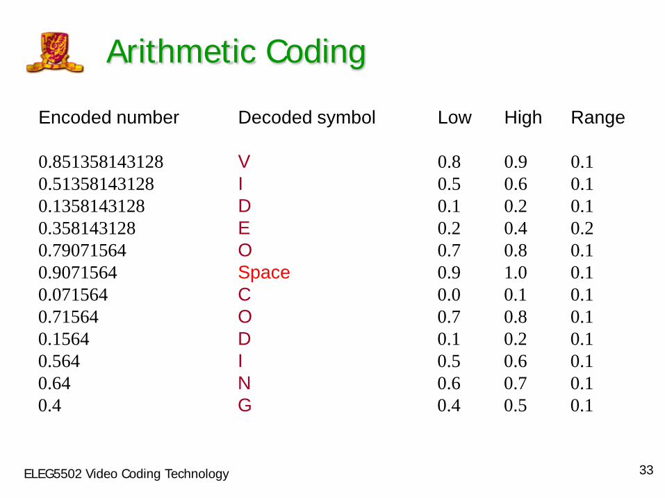
Decoding
• From the encoded number, we can deduce the symbol being transmitted by determining the range which it falls into.
• The next encoded number is given by
where EN is the encoded number.
i
iii RANGE
LOWENEN −=+1
33 ELEG5502 Video Coding Technology
Arithmetic Coding
Encoded number Decoded symbol Low High Range 0.851358143128 V 0.8 0.9 0.1 0.51358143128 I 0.5 0.6 0.1 0.1358143128 D 0.1 0.2 0.1 0.358143128 E 0.2 0.4 0.2 0.79071564 O 0.7 0.8 0.1 0.9071564 Space 0.9 1.0 0.1 0.071564 C 0.0 0.1 0.1 0.71564 O 0.7 0.8 0.1 0.1564 D 0.1 0.2 0.1 0.564 I 0.5 0.6 0.1 0.64 N 0.6 0.7 0.1 0.4 G 0.4 0.5 0.1
34 ELEG5502 Video Coding Technology
Arithmetic Coding
• In the above example, we assigned a predetermined probability to each symbol which is communicated in advance to the encoder and the decoder.
• For a long message, the probabilities are updated as the symbols are transmitted/received at the encoder/decoder. Hence, the model is adaptive, regardless of the starting model.
• There is actually no need to define a starting model at all, particularly for long messages. This is significant because in many cases, this is not available. However, for faster convergence to theoretical entropy bound of compression efficiency, starting model of the symbols' probabilities is required.