1

Quantifying the Effects of Underground Natural Gas Storage on Nearby Residents

Michaela Jellicoe

Department of Agricultural Economics

Purdue University

Michael S. Delgado§

Department of Agricultural Economics

Purdue University

9/29/2014

Michaela Jellicoe, Department of Agricultural Economics, Purdue University, West Lafayette, IN 47907. Email:

mjellico@purdue.edu. § Correspondence to: Michael S. Delgado, Department of Agricultural Economics, Purdue University, West

Lafayette, IN 47907. Email: delgado2@purdue.edu, Phone: 765-494-4211.

We are grateful to Neha Khanna, Juan Sesmero, Gerald Shively and participants at the 2014 NAREA Workshop on

Unconventional Shale Gas and Oil Development for helpful comments. We would also like to thank the Indiana

Geological Survey and the Indiana Department of Natural Resources for providing the data on the locations of

underground natural gas storage activities in Indiana. Maps were created using ArcGIS® software by Esri. ArcGIS®

and ArcMap™ are the intellectual property of Esri and are used herein under license. Copyright © Esri. All rights

reserved. For more information about Esri® software, please visit www.esri.com.

2

Abstract

We estimate the potential negative effects of underground natural gas storage on local residents

using hedonic regression, and a sample of Indiana properties transacted between 2004 and 2013.

We find that underground natural gas storage activities significantly reduce property values.

Property values increase by about 10 percent moving a distance of 1 kilometer away from the

storage field, and each additional storage or observation well located near a property reduces the

property value by about 0.43 and 2.64 percent, respectively. Our research sheds new light on a

previously unexplored aspect of natural gas resource activities.

Keywords: Externalities; Hedonic; Natural Gas Storage.

3

INTRODUCTION

Over the past few years discussion of issues related to natural gas extraction have increased

dramatically in both academic and public domains, often focusing on the potential risks of

hydraulic fracturing. Recent economic research includes studies by Muehlenbachs, Spiller and

Timmins 2012 and Gopalakrishnan and Klaiber 2014. Films like Gasland and The Promised

Land have pulled issues related to hydraulic fracturing and the natural gas industry into the

public eye, as have articles that have appeared in publications like the New York Times and

Forbes. Despite the popularity of these issues, other sectors of the natural gas industry, such as

underground storage of harvested natural gas, have received little attention to date from either

the academic or public arenas. Yet, underground natural gas storage bears many of the same

potential risks as natural gas extraction, including health, environmental, and amenity impacts.

Understanding these potential impacts is important for developing a complete understanding of

the economic impacts of the natural gas industry.

After natural gas is extracted from an underground formation, it is transported via

pipeline to processing plants where it is prepared for consumption. However, not all of the

processed natural gas is immediately consumed; gas that is not consumed is typically stored

underground for future consumption (U.S. Energy Information Administration 2013).

Traditionally, underground natural gas storage served to provide an inventory of harvested

natural gas that can be used to meet peak demand or protect against seasonal differences between

gas extraction and consumption. Now, as natural gas production increases following recent

advances in extraction techniques, the demand for underground storage may also increase for the

following reasons. First, given recent increases in production capacity, it is possible that the

quantity of natural gas produced may exceed available storage capacity. This may be particularly

4

true in times with relatively low consumer demand, as natural gas extraction rates need not

mimic levels of consumer demand. Second, harsh winters like that of 2013-2014 may create

additional demand for natural gas that exceeds available supplies from storage, resulting in an

increase in demand for storage capacity. For instance, a recent (March 2014) Chicago Sun-Times

article reports that levels of natural gas in storage are lower than they have been since 2008

because of high demand during the winter.

Media attention directed at natural gas extraction activities has heightened awareness on

the potential associated risks, often emphasizing risk of ground and surface water contamination.

Like the extraction of natural gas, underground storage poses health and environmental risks,

including (i) migration of the natural gas out of the formation posing the possibility of

contamination of groundwater sources (Miyazaki 2009); (ii) failure of well casings and cement

that protects the formations above and below the well from contamination (this risk could

increase as the well ages) (Miyazaki 2009); (iii) slow leakage from the wellhead (known as off-

gassing), including possible methane emissions (U.S. Environmental Protection Agency 2013);

and (iv) penetration of the formation by another well, including a water well. In addition to

environmental risk, there are also other potential disamenities due to the infrastructure associated

with the storage formation that include (i) noisy compressor stations required to keep the lines

pressurized (Federal Energy Regulatory Commission 2013); and (ii) visual disamenities from

wellheads. These potential disamenities may be reflected in the property values of nearby homes.

We hypothesize that (i) properties located over the storage field have lower property values,

relative to properties not located over the field, and (ii) properties located near underground

storage well sites have lower values, relative to properties located at a distance.

5

We use a hedonic analysis to determine whether these potential disamenities of

underground natural gas storage are significant enough to influence the values of nearby

properties. Hedonic models are commonly applied to issues relating to energy, environmental

quality, and amenity impacts; for instance, the impact on property values of nuclear power plants

(Gamble and Downing 1982), petroleum refineries (Flower and Ragas 1994), hog operations

(Palmquist, Roka and Vukina 1997), water quality (Leggett and Bockstael 2000), and wind

power facilities (Heintzelman and Tuttle 2012). Boxall, Chan and McMillan (2005) find that oil

and gas facilities have significant negative impacts on the values of nearby rural residential

properties, and Weber (2012) finds that the natural gas booms are associated with higher growth

in total employment, and wage and salary income. Guignet (2013) also employs hedonic

methods to estimate the impact of leaking underground petroleum storage on property values,

finding that a leaking underground storage tank has little effect on nearby housing values,

regardless of whether the property relies on private well water.

Recent econometric literature has also examined the impacts of hydraulic fracturing

natural gas extraction on nearby property values, given recent technological advances, increased

attention on the natural gas industry, and potential risks associated with natural gas extraction

(e.g. Muehlenbachs, Spiller and Timmins 2012 and Gopalakrishnan and Klaiber 2014). These

articles also deploy hedonic methods, and both generally conclude that hydraulic fracturing

extraction activities in Pennsylvania negatively impact the values of surrounding homes. Further,

these studies find empirical evidence that risk of groundwater contamination is an important

source of these negative externalities.

We use a semi-log hedonic price function to estimate the impact of proximity and

intensity of nearby underground natural gas storage activity on property values in Indiana.

6

Indiana is an ideal location for assessment of the potential impacts of underground natural gas

storage because storage activities are relatively isolated from other natural resource extraction

activities which allows for more straightforward econometric identification. Our data consists of

a set of 1,512 residential property sales between 2004 and 2013 in 16 counties across Indiana.

We find that property values increase with distance to underground storage activity by about 10

percent per kilometer on average. We further find that each additional storage or observation

well located near a property reduces the property value by about 0.43 and 2.64 percent,

respectively. Additional results demonstrate the properties that have access to public sources of

water are relatively insulated from these negative effects, and that these effects do not

significantly vary with urbanity or the lot size of the property.

BACKGROUND ON UNDERGROUND NATURAL GAS STORAGE

Types of Natural Gas Storage

Underground natural gas storage has been an important aspect of the natural gas industry since

the early 1900s (Federal Energy Regulatory Commission 2004), with processed natural gas

typically being stored in depleted natural gas reservoirs, salt caverns, and depleted aquifers.

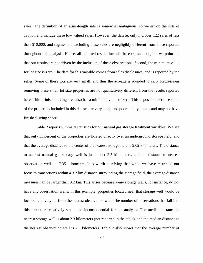
Figure 1 shows the distribution of natural gas storage activities throughout the United States;

depleted natural gas reservoir storage facilities are spread across the United States, while salt

caverns are primarily concentrated in the Gulf Coast and aquifers are concentrated in the Upper

Midwest. According to the U.S. Energy Information Administration (US EIA), total underground

storage capacity in the United States in 2012 was 8,991,335 Million cubic feet, representing the

“present developed maximum operating capacity” (U.S. Energy Information Administration

n.d.). In 2013, storage capacity increased by two percent.

7

In order for an underground formation to be suitable for natural gas storage it must have

certain geologic characteristics, such as a layer of porous and permeable rock where the natural

gas is stored, surrounded by a layer of impermeable rock that stops the migration of the natural

gas out of the porous rock layer (Dawson and Carpenter 1963). The three types of geologic

formations each have different geologic characteristics which impact the capacity and

deliverability of the storage facility. Once a formation is chosen for storage it is reconditioned for

use as a storage facility, and certain aboveground equipment must be installed in order to operate

the storage facility. A storage facility requires wells for injection and withdrawal, as well as

wells for observation and possibly wells for water supply and disposal. Wells include wellhead

valve assemblies, and other equipment that typically includes gathering lines, metering facilities,

compression facilities, dehydration units, and generators or transformers (Federal Energy

Regulatory Commission 2013). Once the underground storage formation is ready for use and the

required equipment has been installed, the gas is injected into the formation through a wellhead

until pressure builds within the formation. This pressure is required in order to allow for the

extraction of the gas at a later time; as a result, there is a certain amount of gas that can never be

extracted, called “cushion” gas (Storage of Natural Gas 2014). The gas contained within the

storage field that is available to be extracted is called “working” gas. Each type of storage well

has different proportions of “working” gas and “cushion” gas, depending on the geology of the

formation, the facility equipment, and operations (U.S. Energy Information Administration

2004).

The most common type of underground formation used for storage is depleted natural gas

or oil reservoirs (U.S. Energy Information Administration 2004). Since these formations have

already held natural gas (or oil), they are known to be capable of storage and the geological

8

structure of these formations is already known (Dawson and Carpenter 1963). Additionally,

depleted reservoirs may already have equipment in place from prior extraction activities, which

potentially reduces the cost of operating the storage facility (Storage of Natural Gas 2014).

Aquifers are another option for underground natural gas storage. While aquifers naturally store

water (so it is likely to be geologically capable of storing natural gas), there is generally less

information on the geological attributes of the formation, and collection of this information can

be costly. Additionally, all of the infrastructure for the storage facility must be developed

(Storage of Natural Gas 2014). Further, the presence of water in the formation requires further

processing of the natural gas once it is removed from the storage facility for consumption, and

also bears increased regulations from the U. S. Environmental Protection Agency (US EPA) to

prevent any groundwater contamination from migration of the stored natural gas out of the

storage facility (Storage of Natural Gas 2014). The third type of underground natural gas storage

formation that is commonly used are salt caverns. Salt caverns have high development costs, due

to the process of clearing the cavern (Federal Energy Regulatory Commission 2004), however,

they are a high deliverability type of facility, making them ideal for emergency and peak load

situations (Storage of Natural Gas 2014).

Demand for Natural Gas Storage

Traditionally demand for natural gas has been seasonal, with peaks in demand occurring in the

winter when natural gas is used for heating. Recent increases in the use of natural gas for

electricity generation has also increased demand for natural gas during summer months. Yet,

production of natural gas is not seasonal. In order to compensate for timing differences between

supply and demand, the natural gas industry uses underground formations to store excess

9

supplies of natural gas when demand is low for later use when demand is high. Recent

advancements in horizontal hydraulic fracturing have greatly increased the efficiency of

production, further increasing the difference between supply and demand. Underground storage

also provides insurance against any unexpected events that could disrupt supply (Storage of

Natural Gas 2014). Finally, since 1994, all interstate pipeline companies operate in “open

access”, allowing third parties to lease working gas capacity which allows them to profit by

withdrawing natural gas from storage when prices are high and storing gas when prices are low

(Storage of Natural Gas 2014).

Natural Gas Storage Legal Requirements

Underground natural gas storage facilities must make certain agreements with landowners

impacted by their activities, similar to those made for the exploration and production of natural

gas. When a company interested in developing underground natural gas storage files an

application with the Federal Energy Regulatory Commission, it must also notify any landowner

that may be impacted by the activity. This includes all landowners located above the geologic

formation in which the gas will be stored (Federal Energy Regulatory Commission 2013). In

addition to notifying impacted landowners of future activity, the pre-filing process required by

the Federal Energy Regulatory Commission includes a program of community outreach, which

includes open houses and other processes to notify all stakeholders of the project and gather

10

input regarding the project from all stakeholders (Federal Energy Regulatory Commission

2012).1

Owners and operators of storage facilities must obtain at the very least the mineral rights

to the underground storage facility. In the case in which the owner or operator does not own the

mineral rights for the underground formation, he/she must establish a storage lease or easement

agreement with the owners of the mineral rights. A previous landowner can attach a storage lease

or agreement to a land deed, and in the case of a property sale or transfer of ownership, a new

property owner can receive compensation for use. In the case in which some surface facilities are

necessary, the company must also obtain a lease or easement for access to these facilities. In the

case that a landowner and the storage company cannot come to an agreement regarding either

mineral rights or surface access, the company can go to court, and in some cases the court can

grant the company the ability to access these rights through eminent domain (Federal Energy

Regulatory Commission 2013).

Potential Risks of Natural Gas Storage

Most of the facilities necessary for underground storage are located underground. As a result,

some landowners may experience little visual impact from the presence of an underground

storage facility. However, the storage company monitors the storage formation through surface

facilities; landowners near the monitoring sites likely experience visual impacts from the storage

1 The Indiana Department of Natural Resources does not require public notice upon the filing of a permit application

for an underground natural gas storage facility for those facilities regulated by the State of Indiana not under the

jurisdiction of the Federal Energy Regulatory Commission (Indiana Department of Natural Resources n.d.c).

11

facility. Other landowners may have compression stations on their property, or be located near a

compression station, and may experience noise impacts. The Federal Energy Regulatory

Commission does have rules regarding acceptable noise levels – in the case of new or modified

compression stations, the noise level cannot exceed an average level of 55 decibels at any “pre-

existing noise sensitive area” (Federal Energy Regulatory Commission 2013). A noise sensitive

area includes areas with schools, hospitals, or residences (Federal Energy Regulatory

Commission 2013).

Beyond the noise and visual impacts related to underground natural gas storage, there are

other potential environmental issues associated with underground natural gas storage. Natural

gas storage poses some risk of migration – i.e. leakage of natural gas from the underground

formation. It is possible that natural gas can migrate out of the formation vertically through

existing wells, despite prior assessments of the structural integrity of the formation. In the event

that a well is leaking, especially in an urban area or area in which homes are located, leaking

natural gas can pose a risk to homeowners via accumulation of natural gas within homes

(Miyazaki 2009).

Over time wells and abandoned wells can degrade, as age can increase the risks of failure

of the wellhead, thereby increasing the risk of migration of the natural gas (Miyazaki 2009).2

2 Miyazaki (2009) cites several examples of wellhead or well casing failure, leakage, and natural gas migration in

recent years. In Colorado, a property owner filed a lawsuit against an underground storage facility in 1998, claiming

that a groundwater aquifer was contaminated by the storage facility. The natural gas had not actually migrated out of

the property included within the underground storage facility, but some quantities of natural gas were discovered in

the aquifer. As a result of this lawsuit the storage facility was decommissioned. The more extreme cases of

migration and risk are linked to salt cavern type storage facilities. One example occurred in Texas in 2004, in which

well casing failure caused an explosion, which led to a second explosion and as a result the loss of between 30 and

12

While federal and state agencies have specific requirements for the construction of natural gas

wells, as well as regulations for the abandonment and plugging of wells, well casings may

corrode over time. This corrosion may lead to natural gas migration as well as migration of

brines from deeper formations into shallower formations (Rupp 2011). This type of migration of

natural gas and brine can pose a risk to sources of groundwater. Further, the working gas in an

underground storage facility can move from high pressure areas to lower pressure areas within

the formation, leading not only to financial losses for the storage operator but also to migration

into other underground formations, including sources of groundwater.

Methane emissions from “off-gassing” at the wellhead or from emissions at the

compressor stations constitute another environmental and health risk associated with natural gas

storage (U.S. Environmental Protection Agency 2013). In addition to emissions, methane from

oil and natural gas formations can contaminate water wells, which is potentially hazardous when

later exposed to the air (i.e. methane in groundwater can be hazardous).3 Although there are no

established federal and state water quality standards for methane in drinking water, there are

60 million dollars of gas, and the temporary evacuation of nearby residents. The consequences of events like these

can range from financial losses to the storage operator and local business, to the evacuation of nearby residents, and

even fatalities. Beyond the damage to companies and residents there are also environmental consequences of these

events, including soil and groundwater contamination. Although salt cavern underground natural gas storage

facilities have had more severe examples of failure in recent years, any negative attention on the risks to nearby

residents due to underground natural gas storage fields can increase risk perceptions for homeowners located near

one of these facilities, even those that are not salt cavern storage facilities.

3 When methane is in concentrations between 5 and 15 percent, it can be ignited by as little as a nearby electrical

outlet. Homeowners relying on well water can educate themselves on the signs of methane in their well water, which

include bubbling noises in the well and gas bubbles in the water.

13

recommendations for safe levels of methane in water (Indiana Department of Natural Resources

n.d.a).

As is clear, underground natural gas storage bears risk of groundwater contamination

from a variety of sources, including natural gas, brine, and methane. Further, many of these

potential risks are similar to those associated with natural gas extraction. Homeowners with

access to a public water system may not experience as high levels of risk for these types of

hazards as federal and state laws require that providers of public drinking water have a schedule

for monitoring and reporting to their state department.4 The US EPA sets standards for

acceptable levels of contaminants as mandated by the Safe Drinking Water Act, which regulates

any public water system that serves greater than 25 people. When a violation of these regulations

occurs, the water provider is required to send out a public notice of the violation. Households

that receive water from any source that serves fewer than 25 people do not have the same level of

protection, and potentially bear substantial risk from underground natural gas storage.

EMPIRICAL METHODOLOGY

The hedonic pricing framework provides a method for measuring the nonmarket value of certain

amenities that are not explicitly traded in a market, by virtue of breaking a traded commodity

(e.g. a house) into a bundle of separate attributes. In addition to physical attributes (e.g.

bedrooms), these attributes may include air quality, water quality, noise, or the perception of risk

from proximity to an underground natural gas storage facility. According to Rosen (1974), the

hedonic hypothesis is that “goods are valued for their utility-bearing attributes or

characteristics.” Using this hypothesis and theoretical framework, and the collection of observed

4 In Indiana, this is the Department of Environmental Management.

14

prices and attributes, it is possible to recover an estimate of a consumer’s marginal willingness to

pay for individual attributes included in the hedonic price function.

The hedonic price function can be linear or nonlinear, and the specification of the

functional form of the hedonic price function is essential in accurately estimating the marginal

willingness to pay (Cropper, Deck and McConnell 1988 and Kuminoff, Parmeter and Pope

2010). Of these forms, the log-linear is one of the most popular (e.g. Taylor 2003 or recent work

by Heintzelman and Tuttle 2012). Additionally, Gopalakrishnan and Klaiber (2014) employ both

a semi-log functional form and a Box-Cox form in the context of natural gas extraction, and find

that both models yield qualitatively similar results. Hence, we follow standard practice and

deploy the log-linear functional form:

ln𝑃𝑖 = 𝛼 + 𝛽𝑧𝑖 + 𝛿𝑥𝑖 + 휀𝑖. (1)

In the hedonic price equation outlined in (1), the index 𝑖 = 1,2, … , 𝑛 denotes housing

observation, 𝛼 represents a constant intercept, 𝑧𝑖 is a vector of natural gas storage treatment

variables, 𝑥𝑖 is a vector of explanatory variables that typically include housing attribute

variables, indicators for spatial (e.g. county or school district) effects, and indicators for year of

sale, and 휀𝑖 is the error term. In our analysis, 𝑧𝑖 contains the variables measuring the impact of

underground natural gas storage, via location over the storage well, proximity to the storage well,

or the intensity of storage activity near the property. We include spatial fixed effects in order to

control for omitted variables bias (Kuminoff, Parmeter and Pope 2010). Inclusion of fixed effects

is one effective means of accounting for unobservables, for instance within a geographic or

spatial region (Heintzelman and Tuttle 2012). We also include time dummies for year of sale to

15

account for unobservable time effects that may influence property values (e.g. the recent

recession). The coefficient estimates on the treatment variables provide a means of recovering

the marginal willingness to pay for amenity or housing attributes (given standard assumptions).

In a log-linear specification, the parameters signify a constant percentage change in price.

DATA

Overview and Construction

In this study, we focus on identification and estimation of the potential negative effects of

underground natural gas storage in the State of Indiana. Some recent studies (e.g. Muehlenbachs,

Spiller and Timmins 2012 and Gopalakrishnan and Klaiber 2014) focus on negative external

effects of hydraulic fracturing in Washington County, Pennsylvania. Although Pennsylvania is

home to underground natural gas storage (see Figure 1), it also is central to hydraulic fracturing

natural gas extraction, as well as coal and oil extraction activities. The presence of these other

activities pose econometric difficulties for identifying and quantifying the value of externalities

associated with a single activity; for instance, it is possible that underground natural gas storage

does not bear significant additional risk for properties already exposed to other natural gas (or

natural resource) activities, or whether such differences can be reliably disentangled

econometrically.5 Hence, it is not clear how underground natural gas storage will impact nearby

properties when operated in close proximity to other natural resource activities. The advantage of

5 Econometric identification has been a large portion of discussion in most recent work on valuing the externalities

associated with hydraulic fracturing in general (e.g. Muehlenbachs, Spiller and Timmins 2012 and Gopalakrishnan

and Klaiber 2014).

16

looking at Indiana is that underground natural gas storage activities are relatively isolated from

other natural resource activities, and we can more reliably develop econometric identification.6

Our dataset consists of a sample of 1,512 single-family residential transactions in 16

counties across the State of Indiana between 2004 and 2013. Each observation constitutes an

arms-length property sale. The counties included in the analysis are Cass, Clark, Daviess,

Decatur, Fulton, Greene, Harrison, Huntington, Knox, Lawrence, Monroe, Pike, Posey, Pulaski,

Randolph, Spencer, Vermillion, and White, and are shown geographically in Figure 2. We have

selected all of the counties in Indiana that are home to underground natural gas storage facilities.

Within each county, we focus on properties that are located directly over and within 3.2

kilometers of the underground storage facility. Figure 3 shows a detailed map of our data in

Monroe County. The central area depicts the underground storage field, while the solid dots

show the location of natural gas storage wells spread over the storage field; the open dots show

the location of natural gas observation wells spread over and nearby the storage field; the

pushpins show the location of properties transacted within proximity to the storage field; and the

larger crosshatched region is our constructed buffer zone in which we focus our analysis. We

have chosen a buffer zone of 3.2 kilometers in order to focus solely on properties that are located

in close enough proximity to the storage field that we might reliably expect to identify any

potential externalities. This distance, however, is not without precedence; recent research

indicates that the effects of natural gas activities are localized to an area of about 3.2 kilometers

(e.g. Boxall, Chan and McMillan 2005, Muehlenbachs, Spiller and Timmins 2012 and

Gopalakrishnan and Klaiber 2014).

6 Indiana does have the potential for unconventional natural gas extraction activities; however, to date those

activities have been relatively limited.

17

Data on natural gas storage and observation wells was obtained from the Indiana

Geological Survey’s Petroleum Database Management System and the Indiana Department of

Natural Resources. In addition to providing a list of wells in the State of Indiana, the data include

details about each well, including construction completion dates, which can be used to determine

the age of the well, and latitudinal and longitudinal coordinates. We use these coordinates to

pinpoint the exact location of each well using ArcGIS software, and overlay the USA Counties

Layer Package from Esri Data & Maps in order to determine which counties within the state

have active underground natural gas storage wells and observation wells. The Indiana Geological

Survey also compiles data on the location, size, and type of underground fields that produce oil

and natural gas. We overlay the well location map on the Petroleum Fields map in order to

determine the location of each underground natural gas or oil formation used to store natural

gas.7

Proximity to natural gas storage activities is commonly used as a continuous measure of

impact, however Guignet (2013) suggests that distance may not be the most accurate measure. In

order to provide a wide range for measures of impact, we include both proximity variables as

well as variables measuring the intensity of natural gas storage activities for each property.

Proximity calculations include the distance to the nearest underground storage field, as well as

the distance to the nearest underground natural gas storage and observation wells. We also create

a binary variable indicating whether the property is located over an underground storage field. In

addition to the proximity treatment variables, we use ArcGIS to count the number of wells within

7 The Petroleum Fields map contains information on natural gas storage activities, in addition to oil resource

operations. Note that the oil resource operations are not generally located in close geographical proximity to

underground storage activities in Indiana.

18

a 3.2 kilometer radius of each property to measure the intensity of natural gas storage activity

near each property. The intensity variables include the number of natural gas storage wells, the

number of observation wells, and the number of both types of wells.

Every county within the State of Indiana is required to collect a sales disclosure form for

each housing transaction that occurs within that county. These sales disclosures are submitted to

the Department of Local Government and Finance, which maintains a database for the entire

state. Using the Sales Disclosure’s online database, we compile a dataset of housing transactions

within the counties with active underground natural gas storage wells. The data collected from

the Department of Local Government and Finance contains the parcel number associated with

each sale, the sale date, the sale price, detailed information about the buyer and seller, and

important notes about each individual sale. We remove all observations that are not classified as

single-family residential homes, as well as $1 sales. These sales are more likely to represent

family or business transactions rather than a market (arms-length) sale. Additionally, all

observations with addresses that the GIS software cannot match to an exact postal address, as

well as any observations that are matched to more than one location, are eliminated. We use GIS

to map each property in relation to the storage activity data.

The data compiled from the sales disclosures does not include any attribute data, or

descriptive data about the house or utilities. The county assessor’s office maintains property

records for every parcel within their county, from which we obtain all of our housing attribute

data for each parcel. The attribute data includes the size of the house in finished square feet, the

size of the property in acres, the number of stories, bedrooms, bathrooms, garages, fireplaces,

pools, whether or not the property has public utilities, the year the house was constructed, and a

quality of construction grade for the home. Recent hedonic pricing analyses on natural gas

19

extraction using hydraulic fracturing have found significant impacts on housing values when the

home does not have access to public water; therefore the variable for public water (also from the

assessor’s office) is of particular importance for this analysis. When a house has access to public

water it does not necessarily mean that the home uses public water, but simply having the ability

to connect with a source of public water potentially mitigates (some of the) risk associated with

groundwater contamination. All observations missing data on these variables were removed.

In addition to the attribute data included in the property report cards we also collect data

on the distance to the nearest street, demographic variables at the census tract level, school

districts, and whether the property is located in an urban area. We define the nearest street as

primary limited-access roads or interstates, primary US and state highways, and secondary state

and county highways. Urban areas include both Census 2010 Urbanized Areas and Urban

Clusters.

Descriptive Statistics

Table 1 provides descriptive statistics for the housing attribute data used in this study. The

average sale price of the properties is $94,559.90, with an average lot size of 1.01 acres and

1664.52 finished square feet. In addition, the average home is just under 57 years old, and is

located about 0.82 kilometers from the nearest road. It is clear from these averages, as well as

our urban indicator, that most (about 70 percent) of these properties are located in rural areas. In

addition, most of the properties are constructed with good or average grade materials, and most

(85 percent) have a garage.

A few details are worth mentioning. First, the minimum sales price is $10. As mentioned

previously all $0 and $1 sales were removed from the dataset, in order to ensure arms-length

20

sales. The definition of an arms-length sale is somewhat ambiguous, so we err on the side of

caution and include these low valued sales. However, the dataset only includes 122 sales of less

than $10,000, and regressions excluding these sales are negligibly different from those reported

throughout this analysis. Hence, all reported results include these transactions, but we point out

that our results are not driven by the inclusion of these observations. Second, the minimum value

for lot size is zero. The data for this variable comes from sales disclosures, and is reported by the

seller. Some of these lots are very small, and thus the acreage is rounded to zero. Regressions

removing these small lot size properties are not qualitatively different from the results reported

here. Third, finished living area also has a minimum value of zero. This is possible because some

of the properties included in this dataset are very small and poor quality homes and may not have

finished living space.

Table 2 reports summary statistics for our natural gas storage treatment variables. We see

that only 11 percent of the properties are located directly over an underground storage field, and

that the average distance to the center of the nearest storage field is 9.02 kilometers. The distance

to nearest natural gas storage well is just under 2.5 kilometers, and the distance to nearest

observation well is 17.35 kilometers. It is worth clarifying that while we have restricted our

focus to transactions within a 3.2 km distance surrounding the storage field, the average distance

measures can be larger than 3.2 km. This arises because some storage wells, for instance, do not

have any observation wells; in this example, properties located near that storage well would be

located relatively far from the nearest observation well. The number of observations that fall into

this group are relatively small and inconsequential for the analysis. The median distance to

nearest storage well is about 2.3 kilometers (not reported in the table), and the median distance to

the nearest observation well is 2.5 kilometers. Table 2 also shows that the average number of

21

storage activity wells (both storage and observation wells) near each property is 15.4, while the

average number of storage wells is 11.62 and the average number of observation wells is 3.78.

RESULTS

Initial Regressions

In order to provide an initial benchmark set of results, we first run a regression using only the

basic hedonic attributes as well as year and county indicators. These results are shown in column

1 of Table 3. The regression results indicate that the hedonic attributes generally have the

expected impact on housing values. As expected, homeowners prefer larger properties and larger

homes of higher quality with more amenities. Estimation results indicate that for an increase in

one acre in lot size, property values see a 3.84 percent increase in value. Additionally, for a one

square foot increase in finished living area, property values see a 0.02 percent increase in value.

Both of these estimates are statistically significant. The height of the home in stories, and the

number of bedrooms and bathrooms, are insignificant, likely indicating that people generally do

not prefer more rooms of smaller size (since square footage is being held constant).

We find that the age of the property is negative and significant, and nonlinear: at a mean

value of 56.97 years, a home sees a decrease in value of 0.51 percent. The turning point at which

a home sees an increase in value due to an additional year can be calculated as 𝑥 = |𝛿1 2𝛿2⁄ |, in

which 𝛿1 is the coefficient on Age and 𝛿2 is the coefficient on Age2. This turning point is 119.5

years, indicating that in general as a home ages it loses value, however once it reaches about 120

years, the property begins to increase in value. The number of fireplaces is positive and

significant, representing a 9.96 percent increase in property value with each additional fireplace.

22

Following Halvorsen and Palmquist’s (1980) interpretation of the impact of dummy

variable coefficients, we can determine the impact of the dummy variables representing different

quality grading for homes. Halvorsen and Palmquist (1980) show that the percentage effect of a

dummy variable on price in a log-linear model can be calculated by 100(𝑒𝛿1 − 1), where 𝛿1 is

the coefficient on the dummy variable. A home with excellent grade building quality sees a

537.7 percent increase in property value over a poor grade home. A good grade home sees a

458.84 percent increase, and an average grade home sees a 215.69 percent increase. The

magnitude of these percent increases is large, however when looked at within the context of the

average price of homes within each group of building quality indicators, the magnitude is

reasonable. Homes within the poor building quality group – the base group – have an average

sale price of $18,120.59. In comparison, the average grade building quality group has an average

sale price of $48,166.06, the good building quality group has an average price of $126,574, and

the excellent grade group has an average sale price of $254,227. Given the enormous difference

in average sale price between poor quality homes and excellent quality homes, a 537.7 percent

increase in value for an excellent home compared to a poor quality home is reasonable.

As seen from regressions reported in Table 3, the impact of the housing attribute

variables on property values are both stable across model specifications, and consistent with our

expectations. In what follows, we focus our attention specifically on the relationship between

underground natural gas storage activity and property values.

Proximity to Underground Storage Activity

We begin our focus on the impact of underground natural gas storage by adding simple linear

proximity treatment variables to the basic hedonic regression. These results are reported in

23

Models 2 through 5 in Table 3. Specifically, we include an indicator for whether the property is

located directly above a natural gas storage field, as well as the distance to nearest gas field,

distance to nearest storage well, and distance to nearest observation well. It is clear from Table 3

that all of these measures are statistically insignificant.

These basic linear functional form results indicate that the impact on housing values due

to underground natural gas storage activity may be insignificant. This would indicate that, while

there are possible negative external effects of underground natural gas storage activity, these

effects are not substantial enough to impact property values. However, a more complex

functional form, including quadratic and cubic terms may be more enlightening if there are

significant nonlinearities that have been neglected in the simple model.

In order to capture potential nonlinear impacts from underground natural gas storage

activities on housing values, we run regressions similar to the basic proximity treatment variable

regressions, this time deploying squared and cubic functional forms. Results from these

regressions are reported in Table 4. The percentage impact on housing values from an additional

meter of distance from any of the proximity treatment variables in the quadratic specification can

be calculated as 100(𝛽1 + 2𝛽2𝑧), in which 𝛽1 is the coefficient of the linear proximity term, 𝛽2

is the coefficient on the quadratic proximity term and z is the proximity term. In the cubic

specification, the percentage impact is calculated as 100(𝛽1+2𝛽2𝑧 + 3𝛽3𝑧2), in which z is the

proximity treatment variable, 𝛽1 is the coefficient on the linear term, 𝛽2 is the coefficient on the

quadratic term, and 𝛽3 is the coefficient on the cubic term. When the functional form is

nonlinear, the impact on housing values is dependent on the distance itself.

In the quadratic model, the proximity to the nearest natural gas field and the distance to

the nearest observation well is insignificant (when considering the significance of the average

24

marginal effect, not individual coefficients), but the distance to the nearest underground natural

gas storage well is significant for both linear and quadratic terms. At a distance of 1 kilometer,

the impact of an additional kilometer of distance increases property values by 9.2 percent. At the

mean distance of about 2.5 kilometers, the impact of an additional kilometer of distance on

property values is 5.13 percent. These results indicate that the impact of underground natural gas

storage wells is not constant and decreasing as distance increases, which is expected since as

distance increases properties are less sensitive to underground storage activity. Additionally,

both terms are jointly statistically significant at a 5 percent level. However the terms become

insignificant when evaluated at the mean distance, which indicates that the impact of

underground natural gas storage wells is quadratic and significant at a distance of 1 kilometer

from a home, but the impact is no longer significant at a distance of 2.5 kilometers or greater.

We plot, in the top panel of Figure 4, the non-constant marginal effect of distance to nearest

storage well on property values. Given the confidence bounds, it is clear that the impact of

proximity to nearest storage well becomes insignificant at a distance of about 1 kilometer. At

shorter distances, the marginal effect is significant.

The nonlinear estimation results clearly indicate that there is a significant nonlinear

impact due to proximity of underground natural gas storage wells. It follows that other types of

wells could have nonlinear impacts as well; therefore we consider a cubic functional form in

Models 4 through 6. We find that the distance to nearest well and the distance to nearest storage

well are insignificant in the cubic specification, but we find that each of the cubic terms are

statistically significant for the distance to nearest observation well in Model 6. At a distance of 1

kilometer, the impact is an increase in property value of 10.03 percent. The three proximity terms

are jointly significant at a distance of 1 kilometer, and at greater distances as well. This indicates

25

that the impact of an observation well on home values is non-constant, and an increase in

distance at 1 kilometer has a positive impact on value. The bottom panel of Figure 4 plots this

marginal effect. Thus, homeowners prefer properties located further from observation wells.

The results reported in Table 4 indicate that both natural gas storage and observation

wells significantly – and negatively – impact property values.

Intensity of Underground Storage Activity

Proximity is one way to measure the impact of underground natural gas storage activity on

nearby property values, however it is possible that a proximity measure is not sufficient for

accurately identifying external effects of underground natural gas storage. Guignet (2013), for

instance, finds that proximity measures may not be the best measure of exposure to

environmental effects. In order to use a different measure of the impact of underground natural

gas storage on nearby property values, we also use models with measures of intensity for natural

gas storage related activities. The measures of intensity we use are counts of different types of

wells within 3.2 kilometers of a property.

Results from the models employing a measure of intensity rather than a proximity

variable are reported in Table 5. The results indicate that higher intensity of underground storage

activity decreases property values, and each are significant at a 10 percent level. An additional

storage related well of any type decreases property values by 0.43 percent. A decrease of 0.43

percent at the mean sale price of $94,559.90 is a loss in value of $406.61, and at the maximum

sale price of $625,000 is a loss of $2,687.50. An additional underground natural gas storage well

leads to a reduction in value of 0.48 percent, and an additional observation well leads to a

reduction in value of 2.64 percent. These results confirm our findings from the proximity

26

measure regressions that underground natural gas storage activity does have a statistically

significant and negative impact on nearby property values.

Interestingly, the impact of observation wells seems to be larger in magnitude than

underground natural gas storage wells. Looking back to Table 2, the average number of storage

wells near a property is 11.62, while the average number of observation wells is 3.78. A

reasonable conjecture might be that storage wells impact property values at a diminishing rate, so

that on average an additional storage well located near a property may appear to have a smaller

impact given that most properties in our data have a larger number of storage wells nearby.

Alternatively, there may be some perceived differences between storage and observation wells

that leads to a larger negative impact of observation wells on property values, relative to the

impact of storage wells. An observation well is used to monitor the storage field, in order to

ensure that no natural gas is migrating out of the formation. The larger magnitude impact of

observation wells may be due to the fact that when the need for monitoring of a facility is

apparent, homeowners experience an increased perception of risk, as compared to the actual

operation of the facility.

Water Source Interactions

Previous literature analyzing the impact of shale gas extraction on nearby property values has

found little impact due to proximity variables alone; however interactions of natural gas activity

with water source reveal that the impact of natural gas extraction activity is more severe for

properties that rely on private sources of water (e.g. Muehlenbachs, Spiller and Timmins 2012).

Underground natural gas storage – similar to natural gas extraction – presents risk for

groundwater contamination, which likely creates greater risk for homeowners relying on well

27

water instead of a public water source that is better monitored. We hypothesize that although the

impact on property values due to proximity of underground natural gas storage appears to be

insignificant in the simple linear models, it is possible that adding an interaction term to the

regressions will show an impact with statistical significance for homes without access to public

water.

Models 1 through 7 in Table 6 show estimation results from interactions between both the

proximity and intensity treatment variables and an indicator for public water access. For these

specifications, when a property has access to public water (𝑧 = 1), the percent impact on

property values can be calculated as %∆𝑝 = 100(𝛽1 + 𝛽3) for the simple equation ln𝑝 = 𝛼 +

𝛽1𝑧 + 𝛽2𝑥 + 𝛽3𝑧𝑥, in which 𝑧 is the proximity treatment variable and 𝑥 is the binary variable for

access to public water. Table 6 shows that interactions between public water access and the

natural gas storage field indicator, the distance to nearest natural gas field, and the distance to

nearest storage well are statistically insignificant. The interaction term between water source and

the distance to the nearest observation well is significant.

The water source interaction with intensity measures are all significant at the 5 percent

level (shown in Models 5 through 7). Note that in these regressions, the intensity measures are all

negative and significant, while the interaction terms are positive and significant. These results

indicate that properties that do not have access to public water experience significantly negative

effects of storage intensity, while properties that do have access to public water experience

substantially smaller impacts. Specifically, an additional storage related well leads to a decrease

of 1.32 percent in nearby property values for properties without access to public water. A home

with public water sees a decrease in value of 0.31 percent for an additional underground natural

gas storage well. Except for observation well intensity, the intensity measures and interaction

28

terms are all jointly insignificant. This implies that homes with access to public water are not

significantly impacted by underground storage related activities.

A home without access to public water sees a decrease in value of 1.32 percent for an

additional storage related well. This percentage loss in value is much larger in magnitude than

for a home with access to public water. At the mean sale price of $94,559.90, this is a $1,248.19

reduction in value. Homes without access to public water see a decrease in value of 1.53 percent

for an additional underground natural gas storage well, and a decrease of 6.12 percent for an

additional observation well. These results demonstrate that homes without access to public water

see statistically significant and larger impacts due to underground natural gas storage activities.

Additional Robustness Checks

So far, we have used proximity and intensity measures to identify and estimate negative impacts

of underground natural gas storage activity on property values. We find that there are statistically

significant negative impacts. To ensure that these results are robust, we consider a variety of

alternative specifications for robustness.

As a robustness check for the county level fixed effects, we employ a set of school

district dummy variables to specify smaller spatial regions, as well as to reflect the impact of

school districts on property values. The primary difference between the county level fixed effects

models and the school district level fixed effects models is the significance of the full bathrooms

variable. This variable is insignificant in the county level fixed effects model, however it

becomes significant at the 5 percent level when school district fixed effects are employed. The

hedonic attribute estimation results remain consistent throughout the different models employed,

including those models where census block demographic variables are included, and are

29

generally consistent in sign and magnitude with prior expectations. Further, the goodness of fit is

nearly identical between the county fixed effects and school district fixed effects models, as are

estimates on the distance to nearest well measures and distance to nearest well interactions with

water source. In our data, school districts are relatively large, so there is not much geographical

difference between our school district effects and the county indicators.

In order to determine if homes in urban areas receive a different impact from proximity to

storage related activities, we interact the proximity treatment variables with a binary variable for

urban area. Results are shown in Table 7. The estimation results indicate that there are

statistically significant interaction effects between proximity and urban areas, and the interaction

effect between natural gas storage wells and observation wells are significant. A home within an

urban area sees a 16.33 percent increase in value due to an increase in distance of 1 kilometer

from the nearest natural gas storage well. The baseline impact of underground natural gas storage

wells is negative, but insignificant.

The impact due to observation well proximity for a home within an urban area is a

decrease of 1.56 percent per kilometer. As with underground natural gas storage wells, the

baseline effect of distance to the nearest observation well is negative, but insignificant. This

indicates that the magnitude of the negative impact of increasing distance to the nearest

observation well is larger for urban homes. In general, we do not find any robustness in the

interaction between well measures and urbanity; it is possible that the potential interactions

between natural gas storage and urbanity are more complex than simple linear interactions.

In order to test for a relationship between the size of the lot associated with a home and

the proximity to a storage related activity, we include an interaction term between the continuous

variable measuring lot size and the continuous proximity treatment variables (Table 8). Parsons

30

(1990) argues that neglecting to weight a treatment effect, or any attribute that is dependent on

location, by lot size may lead to a bias in the estimates of the impact of these attributes. For

example, a larger lot could see a smaller impact from proximity to natural gas storage wells than

a home with a small lot. However, none of these interaction terms are statistically significant.

Additionally, when comparing these results to initial linear proximity treatment results it is clear

that the sign and magnitude of the results from the lot size weighted models are not materially

different from the basic proximity treatment effect regressions. These results indicate that overall

there is little if any interaction between lot size and the proximity treatment effects, and that the

impact of underground natural gas storage on housing values is unlikely to be dependent on the

size of the property in terms of acres.

CONCLUSION

Recent years have seen considerable focus on the natural gas industry and shale gas extraction.

The environmental and amenity risks to properties and nearby residents from natural gas related

activities are not new, however, little attention has been paid to the potential negative effects of

underground natural gas storage activity on nearby residents. As demonstrated by Miyazaki

(2009), underground natural gas storage fields have risks, ranging from mild to extreme.

Although these risks have been publicized upon the occurrence of an event, previous literature

has not attempted to value the impact of these types of facilities on nearby property values. In the

climate of increasing attention to the natural gas industry, quantification of these potential

negative effects of underground natural gas storage seems particularly relevant.

By employing the hedonic method to data on home sales within Indiana, we aim to

recover an estimate of the impact of underground natural gas storage related activities on nearby

31

housing values. Results from county level fixed effects models suggest that there is a negative

impact on property values of underground natural gas storage activity based on both proximity

and intensity measures. In particular, we find that the impact of distance to nearest storage and

observation well are both significantly nonlinear, with their impacts on property values

diminishing over larger distances. We show that natural gas storage intensity is also significant,

with property values significantly declining with marginal increases in the number of gas storage

and observation wells within a 3.2 kilometer distance. Further, we find that observation wells

have a particularly large negative impact on property values, compared to storage wells, perhaps

because they are more visible, or perhaps because in our data homes have a relatively larger

number of storage wells nearby.

Our additional regressions provide several useful insights for policymakers wishing to

further understand the negative effects our baseline models identify. Our results indicate that

properties with access to public water are generally insulated from these negative effects. A

property without access to public water sees a decrease in value of about 1.3 percent – or about

$1,248 on average – for each additional storage well. These results are a general indication that

much of the perceived risk regarding underground natural gas storage activities may be related to

the risk of groundwater contamination. Also, we do not find any evidence that the effects of

natural gas storage on property values significantly varies with urbanity or lot size. Each of these

aspects are important dimensions of public policy related to natural gas storage.

Policymakers and industry participants can use these results in order to improve

regulations related to underground natural gas storage, as well as improve lease agreements with

homeowners for any future development of underground natural gas storage facilities. Within the

current environment of increasing demand for natural gas throughout the year, industry

32

participants may be planning projects related to storage of natural gas. With a more complete

understanding of the impacts of these facilities, industry participants working on the

development of underground storage facilities can be more prepared to account for the full costs

of these facilities, and respond to the environment of increased awareness of industry activities.

In addition, policymakers need to have a complete picture of the impact of the natural gas

industry on nearby residents in order to weigh the costs and benefits of any new or expanded

industry activity. Currently, as the natural gas industry receives more attention, policymakers are

expected to respond to the perception of risk within their constituents and help decide if the

development of new storage facilities outweigh the social costs. Increasing demand for natural

gas may drive the need for new development of underground natural gas storage facilities; these

results can aid policymakers in protecting homeowners from the negative impacts of

underground natural gas storage related activities while also helping the natural gas industry

respond to energy demand throughout the country.

The quantification of impact may also help homeowners and the natural gas industry in

negotiations for mineral rights access. The location of development for any new underground

natural gas storage facility is limited by the geological requirements for the activity; however, a

more complete understanding of the impacts on property values due to these activities can help

the industry and stakeholders in any decisions regarding the development and use of

underground natural gas storage. In addition, with this information about the impacts of

underground natural gas storage on nearby properties, policymakers can have full information

when deciding how to update regulations regarding underground natural gas storage facilities on

private land as needed.

33

APPENDIX

Details On Constructing Figures

The following is a detailed list of Imager and Data source references used in constructing Figures

2 and 3: World Terrain Base from Esri Data & Maps, credits: Esri, USGS and NOAA; USA

Counties from Esri Data & Maps, credits: Esri, TomTom, Department of Commerce, Census

Bureau, U.S. Department of Agriculture (USDA), National Agricultural Statistics Service

(NASS) and United States Central Intelligence Agency; North America Detailed Streets from

Esri Data & Maps, credits: Esri and TomTom; Petroleum Fields from the Petroleum Fields Map

Service by the Indiana Geological Survey (maps.indiana.edu/metadata/Geology/Petroleum-

Fields.html); Underground Natural Gas Storage Well latitude and longitude provided by the

Indiana Department of Natural Resources and the Indiana Geological Survey’s Petroleum

Database Management System; Home Sales addresses collected from the Indiana Department of

Local Government’s Sales Disclosure Database provided by the Indiana Gateway for

Government Units (gatewaysdf.ifionlin.org/Search.aspx).

For further details, please see Jellicoe (2014).

34

REFERENCES

Boxall, P. C., Chan, W. H. and McMillan, M. L., 2005. “The impact of oil and natural gas

facilities on rural residential property values: a spatial hedonic analysis,” Resource and

Energy Economics, 27, 248-269.

Cropper, M. L., Deck, L. B. and McConnell, K. E., 1988. “On the choice of functional form for

hedonic price functions,” Review of Economics and Statistics, 70 (4), 668-675.

Dawson, T. A. and Carpenter, G. L., 1963. “Underground storage of natural gas in Indiana,”

Special Report Number 1, Geological Survey, Indiana Department of Conservation, 33.

Esri. "USA Counties." ArcGIS Online. Esri, July 19, 2013.

Fahey, Jonathan. "Natural gas industry struggles to keep promises." Chicago Sun-Times, March

11, 2014.

Federal Energy Regulatory Commission, 2004. Current State of and Issues Concerning

Underground Natural Gas Storage. Staff Report.

Federal Energy Regulatory Commission, 2012. Frequently Asked Questions (FAQs) Gas Pre-

Filing, accessed April 2014.

Federal Energy Regulatory Commission, 2013. An Interstate Natural Gas Facility on My Land?

What do I Need to Know. Brochure, Washington, DC.

Flower, P. C. and Ragas, W. R., 1994. “The effects of refineries on neighborhood property

values,” Journal of Real Estate Research, 9 (3), 319-338.

Gamble, H. B. and Downing, R. H., 1982. “Effects of nuclear power plants on residential

property values,” Journal of Regional Science, 22 (4), 457-478.

35

Gopalakrishnan, S. and Klaiber, H. A., 2014. “Is the shale energy boom a bust for nearby

residents? Evidence from property values in Pennsylvania,” American Journal of

Agricultural Economics, 96 (1), 43-66.

Guignet, D., 2013. “What do property values really tell us? A hedonic study of underground

storage tanks,” Land Economics, 89 (2), 211-226.

Halvorsen, R. and Palmquist, R., 1980. “The interpretation of dummy variables in

semilogarithmic equations,” American Economic Review, 70 (3), 474-475.

Heintzelman, M. D. and Tuttle, C. M., 2012. “Values in the wind: a hedonic analysis of wind

power facilities,” Land Economics, 88 (3), 571-588.

Indiana Department of Natural Resources. Permits Oil & Gas Permitting, accessed April 2014.

Indiana Department of Natural Resources, b. Methane Gas & Your Water Well A Fact Sheet for

Indiana Water Well Owners. Brochure.

Jellicoe, M., 2014. “Underground natural gas storage: an examination of property values in

Indiana.” Master’s Thesis, Purdue University.

Kuminoff, N. V., Parmeter, C. F. and Pope, J. C., 2010. “Which hedonic models can we trust to

recover the marginal willingness to pay for environmental amenities?” Journal of

Environmental Economics and Management, 60 (3), 145-160.

Leggett, C. G. and Bockstael, N. E., 2000. “Evidence of the effects of water quality on

residential land prices,” Journal of Environmental Economics and Management, 39 (2),

121-144.

Miyazaki, B., 2009. “Well integrity: an overlooked source of risk and liability for underground

natural gas storage. Lessons learned from incidents in the USA.” Geological Society,

London, Special Publications, 313, 163-172.

36

Muehlenbachs, L., Spiller, E. and Timmins, C., 2012. “Shale gas development and property

values: differences across drinking water sources,” NBER Working Paper 18390.

Palmquist, R. B., 1982. “Measuring environmental effects on property values without hedonic

regressions,” Journal of Urban Economics, 11, 333- 347.

Palmquist, R. B., Roka, F. M. and Vukina, T., 1997. “Hog operations, environmental effects, and

residential property values,” Land Economics, 73 (1), 114-124.

Parmeter, C. F. and Pope, J. C., 2012. “Quasi-experiments and hedonic property value

methods,” in Handbook on Experimental Economics and the Environment, by John A.

List and Michael K. Price. Cheltenham, UK, Edward Elgar Publishing.

Parsons, G. R., 1990. “Hedonic prices and public goods: an argument for weighting

locational attributes in hedonic regressions by lot size,” Journal of Urban Economics,

27 (3), 308-321.

Rosen, S., 1974. “Hedonic prices and implicit markets: product differentiation in pure

competition,” Journal of Political Economy, 82 (1), 24-55.

Rupp, J. A., 2011. “Oil and gas - a brief overview of the history of the petroleum industry in

Indiana,” Indiana Geological Survey, accessed March 2014.

Storage of Natural Gas, 2014. NaturalGas.org, accessed February 23, 2014.

Taylor, L. O., 2003. “The hedonic method,” in A Primer on Nonmarket Valuation, by Patricia A.

Champ, Kevin J. Boyle and Thomas C. Brown, Dordrecht: Kluwer Academic Publishers,

331-393.

U.S. Energy Information Administration. “Definitions, Sources and Explanatory Notes,”

accessed March 7, 2014.

37

U.S. Energy Information Administration, 2004. “The basics of underground natural gas

storage,” U.S. Energy Information Administration, accessed February 22, 2014.

U.S. Energy Information Administration, 2012. "U.S. Lower-48 Active Underground Natural

Gas Storage Facilities, by Type (December 31, 2012)." U.S. Energy Information

Administration, accessed March 2014.

U.S. Energy Information Administration, 2013. Natural Gas Explained Delivery and Storage of

Natural Gas, accessed March 2014.

U.S. Environmental Protection Agency, 2013. Natural Gas STAR Program Basic Information,

accessed March 11, 2014.

Weber, J. G., 2012. “The effects of a natural gas boom on employment and income in Colorado,

Texas, and Wyoming,” Energy Economics, 24, 1580-1588.

38

Figure 1: Geographical location of underground natural gas storage activity in the United States

in 2012 by type of underground storage formation (U.S. Energy Information Administration

2012).

39

Figure 2: Geographical location of the counties used in this analysis in the State of Indiana.

40

Figure 3: Map of our data for Monroe County, Indiana. The central shaded area shows the

location of the underground storage field, the solid dots show the natural gas storage wells, the

open dots show the location of observation wells, the pushpins show the location of property

transactions, and the large crosshatched region shows the area of study around the storage field.

41

Figure 4: Plots of the non-constant marginal effects of the distance to nearest storage and

observation wells on property values. Upper and lower 95 percent confidence bounds are placed

above and below the marginal effect at each point.

42

Table 1: Descriptive statistics for housing attribute data

Variable Mean Std Dev Min Max

Sale price ($) 94559.90 2192.91 10 625000

Lot size (acres) 1.01 2.96 0 75.42

Height of home (number of stories) 1.22 0.39 1 3

Finished living area (sq ft) 1664.52 798.91 0 9478

Fireplaces 0.43 0.74 0 4

Bedrooms 2.77 0.80 0 9

Full bathrooms 1.47 0.65 0 5

Half bathrooms 0.23 0.43 0 2

Age of home (years) 56.97 1.05 0 194

Distance to nearest major road (km) 0.82 1.20 0 8.48

Excellent grade building quality indicator 0.08 0.27 0 1

Good grade building quality indicator 0.40 0.49 0 1

Average grade building quality indicator 0.51 0.50 0 1

Poor grade building quality indicator 0.02 0.13 0 1

Urbanized area indicator 0.29 0.45 0 1

Garages 0.85 0.55 0 3

Pools 0.05 0.21 0 1

Public water indicator 0.68 0.47 0 1

43

Table 2: Descriptive statistics for storage treatment variables

Variable Mean Std Dev Min Max

Natural gas storage field indicator 0.11 0.32 0 1.00

Distance to nearest natural gas field (km) 9.02 9.93 0 33.90

Distance to nearest storage well (km) 2.45 1.64 0.05 14.48

Distance to nearest observation well (km) 17.35 30.48 0.02 86.01

Storage intensity measure (storage and obs wells) 15.40 20.06 0 78

Gas storage wells intensity measure 11.62 15.64 0 60

Observation wells intensity measure 3.78 5.25 0 20

44

Table 3: Regression results for preliminary hedonic regression and storage proximity

Variable (1) (2) (3) (4) (5)

0.0384*** 0.0383*** 0.0393*** 0.0384*** 0.0383***

0.0094 0.0094 0.0094 0.0094 0.0094

-0.1262 -0.1278 -0.1195 -0.1261 -0.1262

0.0829 0.0830 0.0831 0.0829 0.0829

0.0002** 0.0002** 0.0002** 0.0002** 0.0002**

0.0001 0.0001 0.0001 0.0001 0.0001

0.0996** 0.0988** 0.1004** 0.0998** 0.0993**

0.0410 0.0410 0.0410 0.0412 0.0411

-0.0034 -0.0017 -0.0060 -0.0034 -0.0035

0.0384 0.0385 0.0384 0.0384 0.0384

0.0975 0.0972 0.0982 0.0975 0.0980

0.0637 0.0637 0.0637 0.0637 0.0638

-0.0120 -0.0122 -0.0111 -0.0119 -0.0126

0.0712 0.0712 0.0712 0.0714 0.0713

-0.0098*** -0.0098*** -0.0101*** -0.0098*** -0.0099***

0.0032 0.0032 0.0032 0.0032 0.0032

0.00004* 0.00004* 0.00004* 0.00004* 0.00004*

0.00002 0.00002 0.00002 0.00002 0.00002

0.00001 0.00001 0.00001 0.00001 0.00001

0.00003 0.00003 0.00003 0.00003 0.00003

1.8527*** 1.8569*** 1.8655*** 1.8523*** 1.8561***

0.2568 0.2570 0.2571 0.2575 0.2580

1.7207*** 1.7231*** 1.7248*** 1.7204*** 1.7224***

0.2219 0.2220 0.2219 0.2223 0.2223

1.1496*** 1.1526*** 1.1481*** 1.1494*** 1.1510***

0.2136 0.2138 0.2136 0.2139 0.2140

-0.2019 -0.2024 -0.2179* -0.2016 -0.1993

0.1282 0.1283 0.1291 0.1289 0.1297

0.2372*** 0.2356*** 0.2387*** 0.2372*** 0.2366***

0.0517 0.0518 0.0517 0.0518 0.0519

0.1129 0.1127 0.1160 0.1131 0.1124

0.1284 0.1285 0.1285 0.1286 0.1285

0.0392 0.0374 0.0341 0.0391 0.0401

0.0816 0.0817 0.0817 0.0818 0.0819

- -0.0666 - - -

- 0.1196 - - -

- - -0.0204 - -

- - 0.0193 - -

- - - -0.0007 -

- - - 0.0259 -

- - - - 0.0034

- - - - 0.0244

R2

0.4393 0.4395 0.4398 0.4393 0.4393

Public water indicator

Lot size (acres)

Height of home (number of stories)

Finished living area (sq ft)

Fireplaces

Bedrooms

Statistical significance at a 1, 5, or 10 percent level denoted with three, two, or one asterisk (***,**,*).

All regressions include county and year dummies, and a constant. The sample size for all regressions is

1,512 observations.

Full bathrooms

Excellent grade building quality indicator

Age of home (years)

Good grade building quality indicator

Average grade building quality indicator

Half bathrooms

Age2

Distance to nearest major road (meters)

Natural gas storage field indicator

Distance to nearest natural gas field (km)

Distance to nearest storage well (km)

Distance to nearest observation well (km)

Urbanized area indicator

Garages

Pools

45

Table 4: Regression results for proximity measures using nonlinear form

Variable (1) (2) (3) (4) (5) (6)

0.0286 - - 0.0434 - -

0.0277 - - 0.0494 - -

- 0.1225*** - - 0.0326 -

- 0.0458 - - 0.0913 -

- - 0.0053 - - 0.1390***

- - 0.0306 - - 0.0457

-0.0026** - - -0.0048 - -

0.0011 - - 0.0062 - -

- -0.0144*** - - 0.0099 -

- 0.0044 - - 0.0217 -

- - 0.0000 - - -0.0164***

- - 0.0003 - - 0.0042

- - - 0.0001 - -

- - - 0.0001 - -

- - - - -0.0014 -

- - - - 0.0012 -

- - - - - 0.0001*

- - - - - 0.0000

R2 0.4421 0.4434 0.4393 0.4421 0.4439 0.4452

Distance to nearest natural gas field cubed

Distance to nearest storage well cubed

Distance to nearest observation well cubed

Statistical significance at a 1, 5, or 10 percent level denoted with three, two, or one asterisk (***,**,*). All

regressions include a full hedonic conditioning set, county and year dummies, and a constant. The sample

size for all regressions is 1,512 observations.

Distance to nearest natural gas field (km)

Distance to nearest storage well (km)

Distance to nearest observation well (km)

Distance to nearest natural gas field squared

Distance to nearest storage well squared

Distance to nearest observation well squared

46

Table 5: Regression results for hedonic models using intensity measures

Variable (1) (2) (3)

-0.0431* - -

0.0241 - -

- -0.0477* -

- 0.0281 -

- - -0.2640*

- - 0.1379

R2 0.4406 0.4404 0.4407

Storage intensity measure (storage and obs wells)

Gas storage wells intensity measure

Observation wells intensity measure

Statistical significance at a 10 percent level denoted with an asterisk (*). All regressions include a full

set of hedonic conditioning variables, county and year dummies, and a constant. The sample size for all

regressions is 1,512 observations. All results reported are scaled by a factor of 10.

47

Table 6: Regression results for models considering water source interactions

Variable (1) (2) (3) (4) (5) (6) (7)

0.0697 -0.0335 -0.0807 0.1164 -0.1308 -0.1189 -0.1047

0.0867 0.1189 0.1254 0.0915 0.1056 0.1047 0.1012

0.1604 - - - - - -

0.2363 - - - - - -

- -0.0227 - - - - -

- 0.0196 - - - - -

- - -0.0280 - - - -

- - 0.0338 - - - -

- - - 0.0012 - - -

- - - 0.0244 - - -

- - - - -0.1320*** - -

- - - - 0.0440 - -

- - - - - -0.1530*** -

- - - - - 0.0543 -

- - - - - - -0.6120**

- - - - - - 0.2015

-0.2670 - - - - - -

0.2396 - - - - - -

- 0.0055 - - - - -

- 0.0070 - - - - -

- - 0.0513 - - - -

- - 0.0407 - - - -

- - - -0.0044* - - -

- - - 0.0024 - - -

- - - - 0.1010** - -

- - - - 0.0418 - -

- - - - - 0.1210** -

- - - - - 0.0534 -

- - - - - - 0.3790**

- - - - - - 0.1601

R2

0.4399 0.4400 0.4399 0.4407 0.4428 0.4424 0.4429

Statistical significance at a 1, 5, or 10 percent level denoted with three, two, or one asterisk (***,**,*). All regressions include

a full hedonic conditioning set, county and year dummies, and a constant. The sample size for all regressions is 1,512

observations. All intensity variable results reported are scaled by a factor of 10.

Observation wells intensity measure X public water

Natural gas storage field indicator X public water

Distance to nearest natural gas field X public water

Distance to nearest storage well X public water

Distance to nearest observation well X public water

Storage intensity measure X public water

Gas storage wells intensity measure X public water

Observation wells intensity measure

Public water indicator

Natural gas storage field indicator

Distance to nearest natural gas field (km)

Distance to nearest natural gas storage well (km)

Distance to nearest observation well (km)

Storage intensity measure (storage and obs wells)

Gas storage wells intensity measure

48

Table 7: Regression results for models considering urban interactions

Variable (1) (2) (3)

-0.0205 - -

0.0193 - -

- -0.0257 -

- 0.0278 -

- - -0.0077

- - 0.0247

0.0070 - -

0.0156 - -

- 0.1890** -

- 0.0760 -

- - -0.0079**

- - 0.0031

R2 0.4398 0.4417 0.4418

Statistical significance at a 5 percent level denoted with two asterisks (**). All

regressions include a full hedonic conditioning set, county and year dummies, and a

constant. The sample size for all regressions is 1,512 observations.

Distance to nearest natural gas field X urban

Distance to nearest storage well X public water

Distance to nearest observation well X urban

Distance to nearest natural gas field (km)

Distance to nearest natural gas storage well (km)

Distance to nearest observation well (km)

49

Table 8: Regression results for models considering lot size interactions

Variable (1) (2) (3) (4)

-0.0475 - - -

0.0956 - - -

- -0.0230 - -

- 0.0210 - -

- - -0.0080 -

- - 0.0290 -

- - - 0.0042

- - - 0.0244

-0.0351 - - -

0.0227 - - -

- 0.0031 - -

- 0.0022 - -

- - 0.0040 -

- - 0.0080 -

- - - 0.0004

- - - 0.0004

R2 0.4052 0.4405 0.4395 0.4396

All regressions include a full hedonic conditioning set, county and year dummies, and

a constant. The sample size for all regressions is 1,512 observations.

Natural gas storage field indicator X lot size

Distance to nearest natural gas field X lot size

Distance to nearest storage well X lot size

Distance to nearest observation well X lot size

Natural gas storage field indicator

Distance to nearest natural gas field (km)

Distance to nearest natural gas storage well (km)

Distance to nearest observation well (km)