UNIVERSITY OF CALIFORNIA, SAN DIEGO

Quadratic Forms and Relative Quadratic Extensions

A dissertation submitted in partial satisfaction of the

requirements for the degree

Doctor of Philosophy

in

Mathematics

by

Michael William Mastropietro

Committee in charge:

Professor Harold M. Stark, ChairProfessor Daniel Arovas

Professor Lawrence Carter

Professor Ronald EvansProfessor Audrey Terras

2000

Copyright

Michael William Mastropietro, 2000

All rights reserved.

The dissertation of Michael William Mastropietro

is approved, and it is acceptable in quality and

form for publication on micro�lm:

Chair

University of California, San Diego

2000

iii

To my Mother and Father

We could use up two Eternities in

learning all that is to be learned about our

own world and the thousands of nations

that have arisen and ourished and

vanished from it. Mathematics alone

would occupy me eight million years.

|Mark Twain.

iv

TABLE OF CONTENTS

Signature Page . . . . . . . . . . . . . . . . . . . . . . . . . . . . . . . . iii

Dedication . . . . . . . . . . . . . . . . . . . . . . . . . . . . . . . . . . . iv

Table of Contents . . . . . . . . . . . . . . . . . . . . . . . . . . . . . . . v

List of Figures . . . . . . . . . . . . . . . . . . . . . . . . . . . . . . . . . vii

List of Tables . . . . . . . . . . . . . . . . . . . . . . . . . . . . . . . . . viii

Vita . . . . . . . . . . . . . . . . . . . . . . . . . . . . . . . . . . . . . . ix

Abstract of the Dissertation . . . . . . . . . . . . . . . . . . . . . . . . . x

1 Preliminaries . . . . . . . . . . . . . . . . . . . . . . . . . . . . . . . . . 11.1 Basic Number Field Concepts . . . . . . . . . . . . . . . . . . . . . 11.2 Quadratic Fields . . . . . . . . . . . . . . . . . . . . . . . . . . . . 3

1.3 Relative Quadratic Extensions . . . . . . . . . . . . . . . . . . . . . 51.4 The Modular Group . . . . . . . . . . . . . . . . . . . . . . . . . . 7

2 Correspondence of forms and ideals . . . . . . . . . . . . . . . . . . . . . 102.1 A Historical Note . . . . . . . . . . . . . . . . . . . . . . . . . . . . 102.2 Binary Quadratic Forms . . . . . . . . . . . . . . . . . . . . . . . . 102.3 Correspondence of Forms and Ideals . . . . . . . . . . . . . . . . . . 11

2.4 Reduction Algorithm . . . . . . . . . . . . . . . . . . . . . . . . . . 13

3 Correspondence of Forms and Ideals in Relative Quadratic Fields . . . . 16

3.1 Quadratic Forms with Ok coe�cients . . . . . . . . . . . . . . . . . 17

3.2 Ideals in k(p�) . . . . . . . . . . . . . . . . . . . . . . . . . . . . . 18

3.3 From ideals to forms . . . . . . . . . . . . . . . . . . . . . . . . . . 19

3.4 From forms to ideals . . . . . . . . . . . . . . . . . . . . . . . . . . 21

3.5 Examples . . . . . . . . . . . . . . . . . . . . . . . . . . . . . . . . 24

4 The Hilbert modular group . . . . . . . . . . . . . . . . . . . . . . . . . 26

4.1 The action of GL2(Ok)++ on H . . . . . . . . . . . . . . . . . . . . 264.2 The fundamental domain of GL2(Ok)++ . . . . . . . . . . . . . . . 27

4.3 Boundary identi�cations . . . . . . . . . . . . . . . . . . . . . . . . 28

v

5 Reducing quadratic forms with Ok coe�cients . . . . . . . . . . . . . . . 32

5.1 Identi�cation of forms with points in H . . . . . . . . . . . . . . . . 32

5.2 Reducing forms with Ok entries . . . . . . . . . . . . . . . . . . . . 33

6 Class Number Calculations . . . . . . . . . . . . . . . . . . . . . . . . . . 34

6.1 Bounding the Search . . . . . . . . . . . . . . . . . . . . . . . . . . 34

6.2 Implementation of Algorithm with KASH . . . . . . . . . . . . . . 34

6.3 Distinguishing points on the boundary . . . . . . . . . . . . . . . . 36

6.4 Examples . . . . . . . . . . . . . . . . . . . . . . . . . . . . . . . . 36

7 The e�ect of +=� forms on the class group . . . . . . . . . . . . . . . . . 40

7.1 Identifying +=+ forms and ideals . . . . . . . . . . . . . . . . . . . 407.2 A family of �elds with even class number . . . . . . . . . . . . . . . 427.3 Class groups with a cyclic factor of Z=2Z . . . . . . . . . . . . . . . 43

8 Prime Discriminants . . . . . . . . . . . . . . . . . . . . . . . . . . . . . 468.1 Prime discriminants for primes of odd norm . . . . . . . . . . . . . 468.2 Narrow class number one quadratic �elds . . . . . . . . . . . . . . . 50

8.3 Narrow class number 2 quadratic �elds . . . . . . . . . . . . . . . . 55

9 Genus Theory . . . . . . . . . . . . . . . . . . . . . . . . . . . . . . . . . 569.1 The genus �eld . . . . . . . . . . . . . . . . . . . . . . . . . . . . . 579.2 Genus characters . . . . . . . . . . . . . . . . . . . . . . . . . . . . 62

Bibliography . . . . . . . . . . . . . . . . . . . . . . . . . . . . . . . . . . . 67

vi

LIST OF FIGURES

1.1 SL2(Z) Fundamental Domain . . . . . . . . . . . . . . . . . . . . . 8

4.1 Translational Fundamental Domain . . . . . . . . . . . . . . . . . . 29

4.2 Unit Boundary in Q(p5) with y2

y1= �+ . . . . . . . . . . . . . . . . 31

4.3 Altered Unit Boundary in Q(p5) with y2

y1= ��1+ . . . . . . . . . . . 31

4.4 Unit Boundary in Q(p5) with y2

y1= ��1+ . . . . . . . . . . . . . . . . 31

9.1 Genus �eld tower . . . . . . . . . . . . . . . . . . . . . . . . . . . . 59

vii

LIST OF TABLES

2.1 Quadratic forms for Q(p�71) . . . . . . . . . . . . . . . . . . . . . 15

6.1 Quadratic forms for Q(p5)(p�19) . . . . . . . . . . . . . . . . . . 37

6.2 Quadratic forms for Q(p3)(p�23) . . . . . . . . . . . . . . . . . . 38

6.3 Quadratic forms for Q(p5)(p�68� 16!) . . . . . . . . . . . . . . . 39

8.1 Prime Discriminants when 2 is prime in k . . . . . . . . . . . . . . 51

8.2 Prime Discriminants when 2 splits in k . . . . . . . . . . . . . . . . 54

8.3 Prime Discriminants in Q(p2). . . . . . . . . . . . . . . . . . . . . 54

9.1 Genera of forms for Q(p5)(p�68 � 16!) . . . . . . . . . . . . . . . 65

viii

VITA

July 21, 1972 Born, Bristol, Pennsylvania

1993 B. S., magna cum laude, Duke University

1994{2000 Teaching assistant, Department of Mathematics,

University of California San Diego

1996 M. A., University of California San Diego

2000 Department of Mathematics Distinguished Teaching

Award for Teaching Assistants

2000 Ph. D., University of California San Diego

ix

ABSTRACT OF THE DISSERTATION

Quadratic Forms and Relative Quadratic Extensions

by

Michael William Mastropietro

Doctor of Philosophy in Mathematics

University of California San Diego, 2000

Professor Harold M. Stark, Chair

Let k be a real quadratic �eld of class number one, and K be a totally complex

extension of k. We investigate the correspondence between ideal classes of K

and binary quadratic forms with Ok entries. We further demonstrate how to

calculate the class number of K by identifying forms with points in the Hilbert

upper half-plane, and using the geometry of the action of the Hilbert modular

group GL2(Ok)++ to �nd a reduced form in each class. Finally, in the case where

k has narrow class number one, we investigate how the class group of K can be

decomposed into genera via quadratic characters.

x

Chapter 1

Preliminaries

1.1 Basic Number Field Concepts

In this �rst section we simply mention the basic concepts of algebraic number

theory which we shall need throughout. For details the reader is referred to [12],

[10].

An algebraic number �eld k is a �nite degree �eld extension of the �eld of

rational numbers Q. If the degree of this extension is n, there are n embeddings of

k into the complex numbers, C . We refer to these embedding as the conjugates of

k, and denote them by k(1); k(2); : : : ; k(n) (where k(1) = k). Likewise, the conjugates

of an element � of k are the images of � in k(i) and are denoted by �(i). We de�ne

the norm and the trace of an element as the product and sum of its conjugates

respectively.

Those elements of k which satisfy a monic irreducible polynomial with integer

coe�cients are called algebraic integers, or simply integers. Those integers which

are in Q will be called rational integers if a distinction is needed. The integers of

k form a ring (which contains Z), denoted Ok.If k is a degree n extension of Q then Ok is an n-dimensional free Zmodule;

that is, there is a collection of n elements of Ok, !1; !2; : : : ; !n, such that any

element of Ok can be written as a Zlinear combination of these elements. We say

1

2

Ok = [!1; !2; : : : ; !n], and call this set an integral basis.

An integral basis for Ok is not unique, but two di�erent integral bases di�er

by a determinant �1 change of variables. In this way we can de�ne an important

invariant of a �eld known as the discriminant.

De�nition Let Ok = [!1; !2; : : : ; !n]. We construct an n � n matrix M whose

i; j entry is !(i)j . Then d = d(k) = (det(M))2 is called the �eld discriminant of k.

Note by the above remarks, the discriminant is independent of choice of integral

basis.

In number �elds, one replaces the usual arithmetic of elements with arithmetic

of ideals.

De�nition An integral ideal, a is a set of elements of Ok which satisfy the fol-

lowing conditions.

1. If �; � 2 a, �+ � 2 a.

2. a � a for all 2 Ok.

Although 0 satis�es these properties, it is not considered an ideal. In general,

one writes a = (�1; �2; : : : ; �t) to mean \the ideal generated by �1; �2; : : : ; �t". In

other words, a is all sets of Ok linear combinations of the �'s. If a is generated by

one element, we say that a is a principal ideal. It turns out that ideals are also n

dimensional free Zmodules, and thus have integral bases. In this case one writes

a = [�1; �2; : : : ; �n] to mean that all elements of a can be expressed as a Zlinear

combination of the �'s.

One can de�ne the product of two ideals a and b by ab = f�� j � 2 a; � 2 bg,and it is an easy exercise to verify that this too is an ideal. Furthermore, one can

de�ne the inverse of an ideal a as follows.

De�nition We de�ne the inverse of an ideal a as the set

a�1 = f� 2 k j 8� 2 a; �� 2 Okg

3

We point out that a�1 satis�es the de�nition of an ideal given above, except

that its elements are not integers. In fact, if we take a �nite product of ideals and

inverses of ideals, this will also satisfy the above conditions. Such products are the

so called fractional ideals of k. In the remainder of this paper, we use the word

ideals to mean both ideals in the usual sense as well as fractional ideals, and when

we refer to an ideal contained in Ok we call it an integral ideal.

In the same manner as we did for elements of k, we can de�ne the conjugates

of an ideal as its images in the conjugate �elds of k. Also we can de�ne the norm

of ideals as the product of the conjugates. The norm of an ideal is an element of

Q, and is in Zif the ideal is integral.

The collection of ideals forms an abelian group under multiplication, where Okis the identity element. The principal ideals form a subgroup of the group of ideals.

The quotient group of ideals modulo principal ideals is called the ideal class group.

De�nition The cardinality of the class group of k is called the class number and

is denoted by h, or h(k) if clari�cation is needed.

If h = 1 then every ideal in k is principal, and the arithmetic of k is as simple

as possible. In general there is a degree h(k) extension of k in which every ideal of

k is principal. This �eld is called the Hilbert class �eld. Thus, the size of h gives

an indication of how well behaved the arithmetic of the �eld is.

1.2 Quadratic Fields

Here we state speci�c results for degree 2 extensions of Q. We let k = Q(pD),

where we can assume D is square free. If D > 0 we say that k is a real quadratic

�eld, while if D < 0 we say k is a complex or imaginary quadratic �eld.

Proposition 1.1 Let k = Q(pD). Ok = [1; !], where

! =

8<:

D if D � 2; 3 (mod 4)

1+pD

2if D � 1 (mod 4).

4

We then immediately have the following.

Proposition 1.2 Let k = Q(pD). Then the discriminant

d(k) =

8<:

4D if D � 2 or 3 (mod 4)

D if D � 1 (mod 4).

Proposition 1.3 Let k be a real quadratic �eld, and let Uk be the group of units

of k. Then Uk = f��n0g; that is, the units are generated by a single element.

By convention, �0 is chosen to be positive and greater than one. We call �0 the

fundamental unit.

We now concentrate on complex quadratic �elds k. Fix k = Q(pd), where

d < 0, is the discriminant of k. A�will denote conjugation in k. Lastly h =

fx + iy j y > 0g, the so called complex upper half plane which we shall consider

more fully in section 1.4.

Proposition 1.4 Let k be a quadratic extension of Q. Any ideal a 2 k has an

integral basis, i.e. a = [�; �]Z. Further any other integral basis of a is of the form �̂

�̂

!= A

�

�

!(1.1)

where A is a 2 � 2 matrix with Zentries such that jdet(A)j = 1.

Proposition 1.5 Let �; � be elements of k such that �

�62 Q. If

� �

�� ��

!=

1 !

1 �!

!M (1.2)

where M is a 2 � 2 matrix with entries from Q. For a = (�; �), N (a) divides

det(M), and N (a) = jdet(M)j if and only if a = [�; �]. Furthermore, if � and �

are chosen such that:

�

�2 h (1.3)

then det(M) > 0, and the absolute value is unnecessary.

5

In fact, an integral basis exists for any �eld extension. If we insist on ordering �

and � as in (1.3) then in Proposition 1.1 det(A) = 1, and the absolute value may

be dropped.

Proposition 1.6 If a = (�; �) then N (a) is the greatest common divisor of the

coe�cients of:

N (�x+ �y) = (�x+ �y)(��x+ ��y) = ���x2 + (��� + ���)xy + � ��y2:

(1.4)

The above is called the norm form.

This is actually only a special case of a more general theorem, the Kronecker

Content Theorem, but all that we shall need. It will be useful also, to write the

norm form:

N (�x+ �y) = N �

y x

� �

�

!!: (1.5)

1.3 Relative Quadratic Extensions

Our main results will be based on quadratic extensions of quadratic �elds of

class number one. In many respects the theory is exactly the same, however,

there are some di�erences. There is, of course, a more general theory of relative

extensions which we will not mention.

IfK is a degree 2 extension of k there are two embeddings (one of course trivial)

of K into the complex numbers which �x k. We refer to these as the relative

conjugate �elds. The images of an element of K are of course called the relative

conjugates. Throughout, we shall often use the adjective relative only when this

needs to be made clear. We then de�ne for all elements of K the relative trace

and norm as the sum and product of the conjugates. Similarly we can de�ne the

relative trace and norm of an ideal of K. These quantities will be ideals of k, and

will be contained in Ok if the ideal is integral.

6

If K is a degree 2 extension of k where h(k) = 1, then the integers of K are

a 2 dimensional free Ok module. In other words, we have OK = [1;]Okand all

elements of OK are Ok linear combinations of 1 and . We call [1;] a relative

integral basis, or simply an integral basis if it is understood that the base �eld is

k. We further insist that is chosen so that 2 h. We now restate propositions

1.4 and 1.5.

Proposition 1.7 Let k be a real quadratic �eld of class number 1, and K be a

complex quadratic extension of k. Any ideal of a of K has a relative integral basis

a = [�; �]. Any other integral basis for a is of the form

�̂

�̂

!= A

�

�

!(1.6)

where A is a 2 � 2 matrix with Ok entries and det(A) = �, a unit. If we insist on

the ordering of � and � such that

�

�2 h; (1.7)

then � > 0.

Proposition 1.8 Let �; � be elements of K such that �

�62 k. If

� �

�� ��

!=

1

1 �

!M (1.8)

then for a = (�; �), N (a) divides (det(M)), and N (a) = (det(M)) if and only if

a = [�; �]Ok. Furthermore, if � and � are chosen as in (1.7) then det(M) > 0.

7

1.4 The Modular Group

When one studies the equivalence of quadratic forms, it is helpful to have an

understanding of the action of 2 � 2 matrices on complex numbers. For a more

detailed treatment, see [11].

Let GL2(R) = f2 x 2 R matrices with det 6= 0g, and let A =

r s

t u

!2

GL2(R). We de�ne the action of A on a complex number z = x+ iy by

Az =

r s

t u

!z =

rz + s

tz + u(1.9)

We will use the following notation:

Az = zA = xA + iyA

It is a straight forward calculation to show that for all matrices.

yA =det(A) y

jtz + uj2 (1.10)

We see that y and yA have the same sign when detA > 0. Thus if we restrict to

positive determinant matrices, the action preserves the complex upper-half plane.

Of fundamental interest to us is the action of a special subgroup of GL2(R) on

h, the modular group SL2(Z).

SL2(Z) = fA 2 GL2(R) with entries in Zand det(A) = 1g:

Notice that I, the identity matrix, and �I both preserve z, and it can be veri�ed

that these are the only SL2(Z) matrices that do so; thus the action is actually one

by PSL2(Z) = SL2(Z)=f�Ig. However, one always abuses notation and refers

to the coset simply by the matrix itself. Because SL2(Z) is a discrete group, it

acts discontinuously on h. If we consider the orbits of points z in h, we can �nd

a closed simply connected region such that every z has exactly one element in its

8

orbit lying in this region. This region is called a fundamental domain. For SL2(Z)

one can describe a particular fundamental domain F in the following manner.

F = fz = x+ iy 2 h j � 1

2< x � 1

2; jzj � 1; if jzj = 1; x � 0g

(1.11)

One can represent F geometrically with the diagram below.

T

S

-1/2 1/2

i

Figure 1.1: SL2(Z) Fundamental Domain

Notice that the boundaries de�ned by x = �12and x = 1

2can be identi�ed

through a translation by one. That is the matrix T =

1 1

0 1

!identi�es the

point z1 = �12+ iy with z2 =

12+ iy. Also, one can show that if jzj = 1, for the

matrix S =

0 �11 0

!, S(x + iy) = �x + iy. Thus S identi�es the left half of

circle jzj = 1 with the right half. These are the only two boundary identi�cations.

There is a simple algorithm which one can use to �nd the image of any z 2 h

in F . In fact, this very algorithm can be used to construct F in the �rst place.

The idea is what Stark calls the highest point method in [11].

1. If Re(z) is outside the range �1=2 < Re(z) � 1=2 apply a series of T = 1 1

0 1

!to translate Re(z) into this range.

9

2. If jzj < 1 apply

0 �11 0

!so that jzj � 1, this will happen by (1.10). If

jzj = 1 make sure Re z � 0 or else apply S one more time.

3. If jRe zj > 1=2, repeat step 1.

This process will terminate, and when it does, we have found the image of z

in F . Notice that special care needs to be taken when the image of z lies on a

boundary.

Chapter 2

Correspondence of forms and

ideals

2.1 A Historical Note

Gauss �rst worked out the idea of equivalence classes of quadratic forms in his

seminal Disquitiones Arithmeticae. It wasn't until Dedekind that the connection

to ideals of quadratic �elds was made. What is presented here is a modernized

version of these classical ideas.

It should be noted also that there is a correspondence between ideal classes

of real quadratic �elds and quadratic forms, which we will not investigate. The

reader is directed to Gauss' original treatment as well as more modern treatments

in [1],[3],[10].

2.2 Binary Quadratic Forms

A binary quadratic form with integer coe�cients is a homogeneous polynomial

of degree two in two variables: Q(x; y) = ax2 + bxy + cy2, with a; b; c 2 Z. Thediscriminant of Q(x; y), denoted disc(Q(x; y)) = b2�4ac. We shall be interested in

the case where disc(Q(x; y)) < 0. In this setting, we consider only those forms for

10

11

which a > 0 which are called positive de�nite, as for all values of (x; y) 6= (0; 0),

Q(x; y) > 0.

One may think of these quadratic forms in terms of matrices since

Q(x; y) =�x y

� a b=2

b=2 c

! x

y

!: (2.1)

We shall often refer to the form as a symmetric matrix.

By making a determinant one change of variables, one can create a form with

di�erent coe�cients which still represents all the same values as the original form.

This leads naturally to a notion of equivalence.

De�nition Two quadratic forms with rational integer coe�cients, Q(x; y) = ax2+

bxy+ cy2; bQ(x; y) = bax2+bbxy+bcy2, are equivalent, denoted, Q(x; y) � bQ(x; y), if a b=2

b=2 c

!= tM

ba bb=2bb=2 bc!M (2.2)

for some matrix M 2 SL2(Z).

2.3 Correspondence of Forms and Ideals

In this section we present the connection between ideal classes and quadratic

forms without proof. Our main results in the following chapter will mirror these

facts, and the proofs given in the next chapter can be modi�ed to work here.

Let k = Q(pd), where d < 0 is the discriminant of k. We let a be an ideal of k,

and a = [�; �] as given by Proposition 1.4. We de�ne a quadratic form associated

with a by using the norm form given in equation (1.4):

Qa(x; y) =1

N (a)N (�x+ �y) (2.3)

=1

N (a)(�x+ �y)(��x+ ��y)

= ax2 + bxy + cy2:

12

Theorem 1.6 gives us that a; b; c 2Z.The norm form is positive de�nite and its discriminant is d; in fact, it is the

key to the correspondence. It can be seen that the equivalence class of Qa(x; y) is

independent of the choice of integral basis for a. Furthermore, for any ideal b in

the same ideal class as a we have Qa(x; y) � Qb(x; y).

For the reverse correspondence, we start with a positive de�nite quadratic form

with integer coe�cients: Q(x; y) = ax2 + bxy + cy2, of discriminant d < 0. We

wish to �nd a corresponding ideal class in k = Q(pd). Let us factor Q(x; y) as:

Q(x; y) = a(x+ �y)(x+ ��y); (2.4)

where

� =b+pd

2a(2.5)

is minus a root of Q(x; 1). Notice that � 2 h. It is easily seen that a� 2 Ok by

noticing b � d (mod 4) along with Proposition 1.1. Therefore the ideal (a; a�) is

integral, and in fact has integral basis [a; a�].

One can show that two equivalent forms lead to ideals that are in the same

ideal class. Further, if we let Q(x; y) = ax2 + bxy + cy2, � be as in (2.5), and

a = [a; a�], then the form Qa(x; y) as de�ned in (2.3) is equal to Q(x; y). In this

manner we have our correspondence. The theorem can be stated as follows:

Theorem 2.1 Let k be an imaginary quadratic �eld of discriminant d. There

exists a one to one correspondence between ideal classes of k and equivalence classes

of positive de�nite binary quadratic forms of discriminant d, where equivalence of

forms is given by equation (2.2).

The correspondence is given by:

a = [�; �] �! 1

N (a)N (�x+ �y);

ax2 + bxy + cy2 �!�a;b+pb2 � 4ac

2

�:

13

2.4 Reduction Algorithm

We now demonstrate a method for systematically choosing representatives of

each form class, and thus calculating the class number of the quadratic �eld of

discriminant d. To do so, we take advantage of one last correspondence: we identify

our forms with points in the complex upper half plane by identifying Q(x; y) with

= ��� = �b+pb2 � 4ac

2a: (2.6)

If we have two forms Q and bQ, such that Q = tM bQM , with M =

r s

t u

!

� 1

�Q

1

!= 0;

� 1

�tM bQM

1

!= 0;

�r + s t + u

� bQ r + s

t + u

!= 0;

�r +s

t +u1� bQ

r +s

t +u

1

!= 0:

Since is not real, t + u 6= 0, and we may divide by this quantity. Since byb we mean the root of bQ(x; y) with y = 1, we see that b =M . So moving from

form to form is equivalent to acting on the roots by linear fractional transformation.

Thus the representative form we choose for any class is the forms whose root lies

inside F .

De�nition Let Q(x; y) be a positive de�nite quadratic form, and be its root

which lies in h. If 2 F , then we say that Q(x; y) is reduced.

We should note that in most treatments of binary quadratic forms, the de�-

nition of a reduced form is given in terms of conditions on the coe�cients, and

14

the connections between reducing forms and linear fractional transformations is

not mentioned. It was this connection, however, which was a motivation for this

research.

To �nd a reduced form equivalent to a given form, we follow the procedure

outlined in section 1.4. We re-present the algorithm in terms of the coe�cients of

the form.

1. If jbj > a applying a series of T =

1 1

0 1

!will translate b by a putting b

in the range �a < b � a.

2. If a > c apply

0 �11 0

!which interchanges a and c. If a = c make sure

b � 0 or else apply one more inversion.

3. If jbj > a, repeat step 1.

Reduced forms satisfy the following conditions:

�a < b � a ; a � c ; if a = c then b � 0:

This is the usual de�nition of reduced forms, of course equivalent to the one pre-

sented above.

We can impose one more condition.

jdj = 4ac� b2

� 4a2 � b2

� 3a2

� 3b2

(2.7)

This leaves us with a �nite number of triples (a; b; c) to check, and hence a way to

count forms. We now give an example.

15

Example

Let us calculate the class number of Q(p�71). By above considerations we need

only consider jbj �q

713� 4. However, since -71 is odd, b = �1;�3. The b's and

the corresponding a's and c's are shown in the table below.

Table 2.1: Quadratic forms for Q(p�71)

b ac = 71+b2

4(a;b; c)

1 18 (1,1,18) (2,1,9) (3,1,6)

-1 18 (2,-1,9) (3,-1,6)

3 20 (4,3,5)

-3 20 (4,-3,5)

It follows that h(Q(p�71) = 7. We can see which ideals these correspond to

using the correspondence Q(x; y) ! [a; a�]. We know that a is the norm of the

ideal, so we have ideals of norms 1, 2, 3 and 4. Since �71 � 1 (mod 8) and �71 � 1

(mod 3), we have the following factorizations

2 = p2 � �p23 = p3 � �p3:

It is easy to see that the forms 2x2 � xy + 9y2, correspond to p2; �p2, and

similarly 3x2�xy+6y2 to p3; �p3. In fact the forms Q1(x; y) = ax2+ bxy+ cy2 and

Q2(x; y) = ax2�bxy+cy2 always correspond to conjugate ideals. One can see this

by noting that �2 = ���1. Thus the ideal for Q2(x; y) is [a;�a��1] = [a; a��1], which

is the conjugate of the ideal for Q1(x; y). We are left now with only the ideals of

norm 4, which, in light of the above remark, are also conjugates. There are only

three ideals of norm 4, namely, (2); p22; �p22. Since (2) is principal, and the principal

class must correspond to x2+ xy+18y2, the last two forms must correspond to p22

and �p22. Our group is cyclic and generated, for example, by p2.

Chapter 3

Correspondence of Forms and

Ideals in Relative Quadratic

Fields

Having sketched the classical theory, we turn our attention to the connection

between ideal classes of a quartic �eld and quadratic forms with real quadratic

integer entries. The motivation being, that once the correspondence is established,

one can use the geometry of GL2(Ok)++ to reduce forms and calculate class num-

bers. Thus, our goal is to formulate a correspondence in the form of a theorem

similar to Theorem 2.1.

We shall see that the basic nature of the correspondence from the last chapter will

remain unchanged, but there will be some new obstacles to contend with along the

way, some of which have interesting consequences.

Throughout the remainder of this chapter we shall make the following assump-

tion. We let k be a real quadratic �eld of class number one, and 0 denote

conjugation in k. Further, denote by �0 the fundamental unit of k, and �+ the

generator of the totally positive units, so that �+ = �0 if N (�0) = 1 and �+ = �20 if

N (�0) = �1.

16

17

3.1 Quadratic Forms with Ok coe�cients

Consider the binary form Q(x; y) = ax2 + bxy + cy2, with a; b; c 2 Ok. Thereis another form which is intimately related to Q(x; y), namely, the conjugate form

Q0(x; y) = a0x2 + b0xy + c0y2. If disc Q(x; y) = �, then disc Q0(x; y) = �0. We shall

consider forms where both � < 0 and �0 < 0. In this case, we say that � is totally

negative and denote this by � � 0.

Since our coe�cients are real numbers, we can still give meaning to positive

de�nite forms, and therefore we take a > 0. However, Q0(x; y) will be either

positive de�nite or negative de�nite, depending on whether a0 > 0 or a0 < 0. If

N (�0) = �1, then we may consider only those forms where a and a0 are positive.

Without units of norm -1, we can only assume that a > 0. We therefore make the

following de�nition.

De�nition Let Q(x; y) = ax2+bxy+cy2, and disc(Q(x; y)) = �� 0. If N (a) > 0

we say Q(x; y) is type +/+. If N (a) < 0 then we say Q(x; y) is type +/-.

As before, it will be helpful to consider a form as a matrix, and we use the form

and the matrix interchangeably. We give the following de�nition of equivalence in

terms of a matrix equation.

De�nition Two quadratic forms, Q(x; y); bQ(x; y), with Ok coe�cients are equiv-

alent, denoted, Q(x; y) � bQ(x; y), ifQ = (�+)

n � tA bQA (3.1)

for some matrix A, with A 2 GL2(Ok)++, and some n 2Z, where

GL2(Ok)++ =

( a b

c d

!ja; b; c; d 2 Ok; ad� bc = �m+

): (3.2)

One might be curious as to why we allow multiplication by totally positive units.

We include this condition because we would like the forms Q(x; y) and �+Q(x; y)

to be equivalent. Although these forms do not have the same discriminant, their

18

discriminants generate the same ideal in Ok, and furthermore, k(pdisc(Q)) and

k(pdisc(�+Q)) are the same �eld.

When �+ = �20, the equivalence of Q and �+Q can be accomplished without the

use of this multiplication:

Q � �0 0

0 �0

!Q

�0 0

0 �0

!= �+ �Q:

However, when N (�0) = 1, there is no matrix in GL2(Ok)++ which acts like mul-

tiplication by �+ = �0 and so the multiplication is necessary.

3.2 Ideals in k(p�)

We now momentarily turn our attention to the ideal side of the correspondence.

Let K = k(p�) with � � 0. We let � denote complex conjugation, that is, the

nontrivial conjugation ofK=k. Throughout, we are going to be faced with choosing

a generator for principal ideals- speci�cally the relative norms of ideals of K. To

deal with this problem, we shall �x a relative integral basis [1;]Okfor OK, where

we have chosen 2 h, and further choose 0 2 h, where [1;0] is a relative integral

basis for the conjugate �eld. All de�nitions will then depend on this choice of

basis. We shall choose as the generator of the relative �eld discriminant

�(K=k) = � = det

�����

1

1 �

!�����2

; (3.3)

and will use � in all calculations.

We have by Proposition 1.7 that ideals of K have relative integral bases. In

addition, if a = [�; �]Ok, then the conjugate ideal a0 = [�0; �0]Ok

. In light of

Proposition 1.8, we choose det(M) as the generator of N (a), and det(M 0) as the

generator for N (a0) to be used in all calculations. We point out that for a principal

ideal ( ), this method of choosing a generator gives N (( )) = N ( ). In other

19

words, we use the norm of an element as the generator of the norm of the ideal

generated by that element.

Finally, we will always order � and � such that �

�2 h. If N (�0) = �1, then

we can further require that �0

�02 h. If on the other hand, N (�0) = 1, there are two

distinct cases, as with our forms.

De�nition When N (�0) = �1, let a be an ideal of K, with a = [�; �] such that

�

�2 h. If �0

�02 h we say that a is a type +/+ ideal. If �0

�062 h we say a is a type

+/- ideal.

3.3 From ideals to forms

We shall now begin to set up the correspondence between forms and ideals. We

start by identifying an ideal of K with a quadratic form. This is accomplished by

identifying a = [�; �] = [1;]M with Qa(x; y) where:

Qa(x; y) =1

N (a)N (�x + �y)

=1

detMN (�x + �y) (3.4)

= ax2 + bxy + cy2:

The Kronecker Content Theorem assures us that a; b; c 2 Ok. We now prove a

series of propositions which will help us prove the correspondence theorem.

Proposition 3.1 Qa(x; y) has discriminant �, where � is given in (3.3).

Proof.

b2 � 4ac =1

N (a)2(��� + ���)2 � 4���� ��)

=1

N (a)2(��� � ���)2

= �:

20

The last equality comes from taking determinants in (1.8) and the fact we are

using det(M) as the value of N (a). 2

Proposition 3.2 The equivalence class of Qa(x; y) is independent of choice of

integral basis for a.

Proof.

Let a = [b�; b�], be a second integral basis for a, with [b�; b�] = [1;]cM .

bQ(bx; by) = babx2 +bbbxby + bcby2 = 1

detcMN � by bx �

b�b�!!

:

We have by Proposition 1.6, b�b�!= A

�

�

!

where det A = �. Therefore

bQ(bx; by) = 1

detA det MN � by bx �A

�

�

!!:

By making the determinant � change of variables�y x

�=� by bx �A

we have

bQ(bx; by) � 1

detA detMN �

y x

� �

�

!!

=1

�Q(x; y):

Since equivalence of forms allows for multiplication by a totally positive unit,

bQ(bx; by) � Q(x; y):2

21

One can see that without allowing equivalent forms to di�er by a totally positive

unit, when �+ = �0, two di�erent choice of basis for the same ideal would lead to

two inequivalent forms.

Proposition 3.3 Let b and a be two ideals of K in the same ideal class. Then

Qa(x; y) � Qb(x; y).

Proof.

If b is an ideal in the same class as a, b = ( )a, for some ; so if a = [�; �],

b = [ �; �], thus:

Qb(x; y) =1

N (b)N ( �x+ �y)

=1

N (( )a)N ( )N (�x + �y)

=1

N (a)N (�x+ �y)

= Qa(x; y):

2

3.4 From forms to ideals

Given a quadratic form Q(x; y) = ax2 + bxy + cy2 of discriminant �, we will

identify it with an ideal of K by

Q(x; y)! a = (a; a�); (3.5)

where

� =b+p�

2a:

It can be shown that a� is an element of OK. In fact it is an easy calculation

to verify that a� satis�es the polynomial x2 + bx + b2��4, and since � = b2 � 4ac

implies b2�d4

is an integer, a� satis�es a monic polynomial with integer coe�cients.

22

Again, we shall prove a series of propositions concerning the relationship of forms

to ideals which we need to prove Theorem 3.7.

Proposition 3.4 (a; a�) = [a; a�]Ok.

Proof.

Let a = (a; a�). By Proposition 1.6, N (a) is the greatest common divisor of

the coe�cients of N (ax + a�y) = aQ(x; y). Thus, N (a) = a � gcd(a; b; c), anda j N (a). Also, by Proposition 1.8 N (a) j det(M) where:

a a�

a a��

!=

1 !

1 �!

!M:

Taking determinants and squaring we see

(a2�� � a2�)2 = � det(M)2;

a2� = � det(M)2;

a2 = det(M)2;

a = det(M):

Thus we have a jN (a) j det(M) = a, so N (a) = det(M), and by Proposition 1.8

(a; a�) = [a; a�]. 2

We now verify that the ideal class given by (3.5) is independent of the repre-

sentative of the form class.

Proposition 3.5 Let Q(x; y) and bQ(x; y) be equivalent forms with Ok coe�cients,

with corresponding ideals a = [a; a�], and ba = [ba;bab�]. Then a and ba are in the same

ideal class.

Proof.

We de�ne as in (2.6),

= ��� = �b+p�

2a:

23

Noting that Q( ; 1) = 0, we have

� 1

� a b=2

b=2 c

!

1

!= 0: (3.6)

Now if M =

r s

t u

!is the matrix that takes bQ(x; y) to Q(x; y), we saw in

section 2.4 that b =M .

Also,

b� = �(b ) = �(r � + s)

t � + u=

r(� � )� s�t(� � ) + u

=r� � s�t�+ u

:

As a result, a = [a; a�] and ba = [ba;bab�] are in the same ideal class, because r �s�t u

! a�

a

!= C �

bab�ba!; where C =

a (�t�+ u)ba ;

so that [a; a�] and C � ba are the same ideal. 2

Proposition 3.6 Let Q(x; y) = ax2+bxy+cy2 = (x+�y)(x+��y); and a = [a; a�].

Then Q(x; y) = Qa(x; y). Thus, equations (3.7) and (3.8) below are inverses.

Proof.

From equation (3.4) we see:

Qa(x; y) =1

N (a)N (ax+ a�y)

=1

a(a2x2 + abxy + acy2)

= ax2 + bxy + cy2

= Q(x; y):

2

We are now in a position to state and prove the theorem which which was the

goal of the chapter.

24

Theorem 3.7 Let k be a class number 1 real quadratic �eld, and let K be a totally

complex quadratic extension of k. Let � be a generator of the discriminant of K=k

chosen as in (3.3).There exists a one to one correspondence between ideal classes

in K and equivalence classes of positive de�nite quadratic forms with coe�cients

in Ok and discriminant �2�, where � is a totally positive unit, and equivalence of

quadratic forms is given in (3.1). The correspondence is given by the following two

maps,

a = [�; �] �! 1

N (a)N (�x+ �y); (3.7)

ax2 + bxy + cy2 �!�a;b+pb2 � 4ac

2

�: (3.8)

Proof.

Let us verify that the sequence of propositions from this chapter give us our re-

sult. First we have seen that equation (3.7) does in fact give a form of discriminant

� by Proposition 3.1, and (3.8) gives an ideal class in k(p�). Further, the equiva-

lence class of the form in (3.7) is independent of the choice of representative of an

ideal class by Proposition 3.3, and also independent of the choice of integral basis

for that ideal from Proposition 3.2. Conversely, the ideal class of the ideal in (3.8)

is independent of the choice of the form from an equivalence class by Proposition

3.5. Finally, Proposition 3.6 gives us that (3.7) and (3.8) are inverses, completing

the theorem. 2

3.5 Examples

We will now give two examples explicitly giving the identi�cation between

quadratic forms and ideals. The �rst example has �+ = �20 where all ideals are

+=+. The second example has �+ = �0, and an example of both a +=� and a +=+

25

ideal are given. We will be using some facts about factoring ideals and �nding

integral bases for ideals which are useful only in constructing examples. For more

insight one should consult [10] or [3].

Example 1

k = Q(p5), Ok =

h1; 1+

p5

2

iZ= [1; !], �0 = !, �+ = �20.

K = k(p�19), OK =

h1; 1+

p�192

iOk

= [1;].

We factor the ideal (19) in k as (19) = p19p019. Further in K, p19 = P2

19 and we

have

P19 = [4 + !;�63� 18! + ]Ok:

The corresponding norm form is

(4 + !)x2 + (�125 � 36!)xy + (979 + 319!)y2:

If we started with the form 7x2� 3xy+ y2, we see that this corresponds to the

ideal P7 = [7; 3+p�192

] = [7; 1 + ], where (7) is prime in k and (7) = P7�P7 in K.

Example 2

k = Q(p3), Ok = [1; 3]Z= [1; !], �0 = �+ = 2 + !:

K = k(p�23), OK =

h1; 1+

p�232

iOk

= [1;].

In k, the ideal (47) = p47p047; p47 = P47

�P47, and p047 = P047�P047, where we may

take

P47 = [�1 + 4!;�161 � 23! + ]:

Notice that this is a +=� ideal. The corresponding norm form is

(�1 + 4!)x2 + (321 � 46!)xy + (2467 + 2485!)y2:

Also in k, (29) is prime, and in K (29) = P29�P29.

P29 = [29; 387 + 87! + ]

This is a +=+ ideal. The norm form is

29x2 + (775 + 174!)xy + (5961 + 2325!)y2:

Chapter 4

The Hilbert modular group

The notion of the action of SL2(Z) on h can be generalized to the case of the

general number �eld. We shall be interested in the action of GL2(Ok)++ where k is

a real quadratic �eld, and in particular how to use this action to reduce quadratic

forms and compute class numbers. For a detailed treatment of the general number

�eld case, see [11].

4.1 The action of GL2(Ok)++ on H

For a real quadratic �eld k, the natural action of GL2(Ok)++ is on H = h� h.

For z = (z1; z2) = (x1 + iy1; x2 + iy2), the action is given by:

a b

c d

!z =

a b

c d

!(z1; z2) =

a b

c d

!z1;

a0 b0

c0 d0

!z2

!;

(4.1)

where 0 is used to denote conjugation in k, and the action is the usual GL2(R)

action on h as de�ned in (1.9).

If k has fundamental unit of norm -1, then this action is the same as the

action of determinant 1 matrices. For if A 2 GL2(Ok)++, and det(A) = �2n0 , then

26

27

A =

�n0 0

0 �n0

!A0, where det(A0) = 1. Therefore,

Az =

�n0 0

0 �n0

!A0z = A0z;

since it is clear from (4.1) that scalar matrices act trivially. Such a decomposition

is not possible when N (�0) = 1.

It will be useful to treat z1 and z2 as conjugates in the formal sense. We de�ne

a formal norm for all � 2 Ok and z 2 H,

N (�z) = (�z1)(�0z2):

We have that

jN (z)j2 = jz1z2j2 = (x21 + y21)(x22 + y22):

By the \height" of an element z 2 H we shall mean

N (y) = jy1y2j: (4.2)

One may derive the following formula, similar to (1.10):

N (Ay) =N (ad � bc)N (y)

jN (cz + d)j2 : (4.3)

4.2 The fundamental domain of GL2(Ok)++

Following the method demonstrated by Stark in [11], One can construct a fun-

damental domain for GL2(Ok)++ by the \highest point method." This essentially

involves the following.

1. By use of

�+ 0

0 1

!one can �x the value of N (y), while altering the values

of y1; y2 such that ��1+ � jy1y2 j � �+.

28

2. By applying

1 �

0 1

!matrices one can put (x1; x2) inside a parallelogram

(or other suitably chosen region) determined by 1 and !.

3. By (4.3) we see that when jN (cz + d)j < 1 we raise the height of z. This is

equivalent to the condition that����N�z+

d

c

����� <���� 1

N (c)

���� :We think of this collection of points as the \sphere" centered at �d

cof \ra-

dius" j 1N (c)j. There will be a collection of such spheres which will form the

oor of the fundamental domain. According to Cohn in [5], Q(p5) is the

only �eld that has only spheres of radius 1. Because of this, the oor is a

complicated structure, and not easily examined in general. This is a problem

which will be confronted in what is to come.

4.3 Boundary identi�cations

The fundamental domains for three small real quadratic �elds were worked out

by Claus in [2]. However, he does not consider the boundary identi�cations. He

does suggest, like Cohn, that the oor is a complicated structure. To be able to

reduce forms and calculate class numbers, it will be necessary to know when two

forms are equivalent. For this reason, we need to at the very least observe the

nature of the boundary identi�cations.

It turns out that the three types of boundaries mentioned above (corresponding

to each step in the reduction) identify with only boundaries of the same type- that

is, translational boundaries identify with translational boundaries, unit boundaries

with unit boundaries, and oor boundaries with oor boundaries.

This is fairly clear for the translational boundaries. If Ok = [1; !], the two

fundamental translations are T1 = (1; 1) and T2 = (!; !0). If one centers a par-

allelogram about the origin in the x1x2 plane, one gets the following boundary

conditions associated with translations:

29

X1

X2

1

T

T

2

Figure 4.1: Translational Fundamental Domain

�! � !0

2� x2 � x1 < ! � !0

2;�! � !

0

2� !x2 � !0x1 < ! � !0

2

Obviously, opposite sides of the parallelogram are equivalent under the appropriate

translation, as shown in Figure 4.1.

The second type of boundary occurs when z is in the interior of the parallelo-

gram, above the oor, and jy1y2j = ��1+ or jy1

y2= �+j. These two regions identify with

each other in pieces in the following way. Suppose z = (z1; z2) andy1y2= ��1+ . Now

consider the point z� =

�+ 0

0 1

!z. We have

����y�1y�2���� =

���� �+y1�+0y2

����= �2+

����y1y2����

= �+:

If jN (cz+ d��1+ )j > 1 then jN (cz� + d)j > 1, since these two norms are equal;

i.e., if z was above the oor, then so is z�. However, z� is probably no longer

30

inside the fundamental domain for translations. Let us investigate what happens

to (x1; x2). Observe x1 is stretched by a factor of �+ (which is greater than 1),

and x2 is compressed by a factor of �+0 (which is less than 1). Our parallelogram

becomes skewed. This skewed parallelogram is translationally equivalent to our

original parallelogram in polygonal pieces. This is illustrated in Figures 4.2, 4.3,

and 4.4.

Of course, the region need not be a parallelogram, but only a translational

fundamental domain. The only concern one would have is that two pieces may

overlap. This is not possible. Let x;w be two points in the interior FT (we have

dealt with the boundary of the parallelogram). If �+x = �+w+� for some �, (that

is, two points in the skewed parallelogram are translationally equivalent), then we

would have x = w + (�+)0� making x and w translationally equivalent, which is

impossible, as they are in the interior of the parallelogram.

We are left only with the oor, which by exhaustion, must identify with itself.

In what manner this occurs, however, is not easily seen. We have not found any way

to consider the oor as to �nd all the boundary identi�cations. Part of the problem

is a visualization one- the oor is a three dimensional object which occupies four

dimensions. More serious however is the complexity of the oor, which Cohn

examined in [5]. The result of this complexity is that special care must be taken

to distinguish whether two points on the oor boundary are equivalent. We shall

mention how to deal with this problem in terms of our forms in a later section.

31

X1

X2

Figure 4.2: Unit Boundary in Q(p5) with y2

y1= �+

X1

X2

Figure 4.3: Altered Unit Boundary in Q(p5) with y2

y1= ��1+

X1

X2

Figure 4.4: Unit Boundary in Q(p5) with y2

y1= ��1+

Chapter 5

Reducing quadratic forms with

Ok coe�cients

5.1 Identi�cation of forms with points in HWe will now demonstrate how to pick a representative quadratic form in each

equivalence class. We saw how quadratic forms with negative discriminant could

be identi�ed with a point in the complex upper half plane. In a similar manner

we now identify our new forms with a point in the Hilbert upper half plane by

ax2 + bxy + cy2 ! �b+

p�

2a;�b0 +

p�0

2a0

!: (5.1)

Some care needs to be taken when �+ = �0, since in this case there may be

+=� forms. When this occurs, we are identifying such a form with a point in

h � h� (by h� we mean fx + iy 2 C j y < 0g). Of course, GL2(Ok)++ acts on

this set as well, and it will send points in h � h� to points in h � h�. It turns

out that one may use the same conditions to describe a fundamental domain for

this action as well. Obviously, the translational boundaries are not e�ected. One

can still use the same unit boundary condition, with the understanding that the

ratio is to be taken positively. Finally, by taking the absolute value of the height,

32

33

we will be able to construct the same highest point fundamental domain that we

used for the action on H = h� h. Equivalently, we may identify a +=� form with��b+

p�

2a; �b

0�p�0

2a0

�, which is in H.

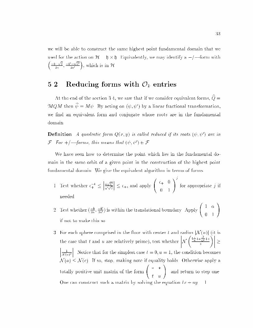
5.2 Reducing forms with Ok entries

At the end of the section 3.4, we saw that if we consider equivalent forms, bQ =

tMQM then b = M . By acting on ( ; 0) by a linear fractional transformation,

we �nd an equivalent form and conjugate whose roots are in the fundamental

domain.

De�nition A quadratic form Q(x; y) is called reduced if its roots ( ; 0) are in

F . For +=� forms, this means that ( ; � 0) 2 F .

We have seen how to determine the point which lies in the fundamental do-

main in the same orbit of a given point in the construction of the highest point

fundamental domain. We give the equivalent algorithm in terms of forms.

1. Test whether ��1+ ����ap�0a0p�

��� � �+, and apply

�+ 0

0 1

!j

for appropriate j if

needed.

2. Test whether (�b2a; �b

0

2a0) is within the translational boundary. Apply

1 �

0 1

!

if not to make this so.

3. For each sphere comprised in the oor with center t and radius jN (u)j (it isthe case that t and u are relatively prime), test whether

����N�b tu+a t2

u2+c

a

����� ���� 1N (u)2

���. Notice that for the simplest case t = 0; u = 1, the condition becomes

N (a) � N (c). If so, stop, making note if equality holds. Otherwise apply a

totally positive unit matrix of the form

� �t u

!. and return to step one.

One can construct such a matrix by solving the equation tx+ uy = 1.

Chapter 6

Class Number Calculations

6.1 Bounding the Search

In order to use our forms to calculate class numbers, we would like some bound

on our search region, analogous to the condition b <

qjdj3in the classical case.

We do this by noting that the oor of the fundamental domain bounds N (y)

su�ciently away from zero. Also, since the ratio of y1 and y2 is bounded, we can

�nd a minimal value M for y1. This means that

M �p�

2aso that

a �p�

M:

One can further use the relation between b and a from the translational fundamen-

tal domain in turn to get a maximal value for b. Cohn in [4] found values for the

lowest points in the fundamental domains which were useful in computation.

6.2 Implementation of Algorithm with KASH

In order to expedite the calculations, the algorithm was implemented using

KASH v. 1.9 [6], an algebraic number theory package developed at T.U. Berlin.

34

35

Programs were written to both reduce forms and make class number calculations.

There is a certain amount of initialization that must be done which depends on

the �eld. We restricted to the cases of k = Q(p3) and k = Q(

p5) which cover

both the unit of norm 1 and -1 cases respectively. The initial parameters needed

were

1. An integral basis for Ok.

2. The fundamental unit of Ok.

3. The spheres comprising the oor of the fundamental domain for GL2(Ok)++,

taken from [2].

4. A bound for M , the minimal value of y1, from [4].

With those parameters in place, one does the following.

1. For all possible b, one factors the ideal j�j+b24

= ac where N (a) � N (c) using

the KASH function IdealFactors.

2. One then �nds a positive generator a of the ideal a, which satis�es the unit

boundary conditions. Notice that at most one can possibly work.

3. Find the number c = b2+j�j4a

, and create the form ax2 + bxy + cy2.

4. If the form is reduced, add it to the list of reduced forms, and note if form

is on a oor boundary.

5. When complete, check to see if forms on oor are equivalent.

The last step is non-trivial and deserves elaboration, which we provide in the

next section.

36

6.3 Distinguishing points on the boundary

As we have noted, the oor boundaries are not very easy to study, and as a

result the boundary relations related to the oor are not known. This presents a

problem when counting reduced forms as we must determine whether two forms

on the boundary are equivalent. The following method was used to determine

equivalence of forms on the boundary.

There are two obvious ways 2 forms on the boundary can be equivalent. The

�rst way is for the two forms to correspond to conjugate ideals, a and �a, where

a has order 2 in the class group. Since N (a) = a�a is principal, [�a] = [a�1], so if

a has order 2, [a] = [a�1] = [�a]. It is an easy matter to test this for all forms on

the boundary. We �nd the ideal a corresponding to the form on the boundary and

�nd Qa2(x; y) as in (3.8). We reduce this form, and if it is the principal form, our

original form has order two. We shall see an example shortly.

The second way for two forms to be equivalent, is if they are related by the

change of variables (x; y)! (�y; x). In terms of forms, we will see ax2+ bxy+ cy2

and cx2 � bxy + ay2. This can be done by inspection instantly.

If this is insu�cient, one can of course exhaustively check whether or not two

forms are equivalent. Empirically, it was rarely the case that this was needed.

6.4 Examples

We use the same �elds as we did in the examples at the end of chapter 4.

Example 1

k = Q(p5), K = k(

p�19).We use all the same notation as in Example 1 from section 3.5. The fundamental

domain of GL2(Ok)++ is given by the relations

p5

2� x2 � x1 <

p5

2;

p5

2� !x2 � !0x1 <

p5

2;

37

!�2 � y2

y1< !2;

N (z) � 1; N (z � 1) � 1; N (z � !) � 1; N (z � !0) � 1:

Cohn in [4] gives 514

2!as a bound for the minimum value of y1.

Table 6.1 shows the reduced forms returned by the KASH program. Notice that

the two forms on the boundary are conjugates, and correspond to the factors of 5

in K. An easy calculation shows that they are order two, and thus equivalent. The

class number of K is four. Our group is either Z=2Z�Z=2Zor Z=4Z, dependingon whether (2;�1 + 2!; 3) has order 2 or not. If the corresponding ideal is P2,

we compute P22, and use 3.7 to give the equivalent form. The reduction algorithm

does not return the principal form and thus the class group is Z=4Z.

(a;b; c) On Sphere

(1; 1; 5)

(2 + !;�1; 3� !) 0

(2 + !; 1; 3 � !) 0

(2;�1 + 2!; 3)

(2; 1 + 2!; 3 + !)

Table 6.1: Quadratic forms for Q(p5)(p�19)

Example 2

k = Q(p3), K = k(

p�23).The fundamental domain is given by the relations

�p3 � x2 � x1 <

p3; �1 � x2 + x1 < 1;

�+ � y2

y1< �+;

N (z) � 1; N (z�1) � 1; N (z�p3) � 1; N (z�

p3�2) � 1; N (z�

p3�2) � 1;

N z +�1�

p3

2

!� 1

4;

38

N�z � 1p

3

�� 1

9; N

�z � 2p

3

�� 1

9:

Again from [4] we have

p2�p3

2as a bound for the minimum value of y1.

Of the 15 forms in the Table 6.2, six are on the boundary. These are equivalent

in conjugate pairs, as each of the forms has order 2. The class number is thus 12.

The class group is one of the two following groups:

Z=12Z;Z=2Z�Z=6Z:

Since Z=12Zhas only 1 element of order 2, the group is Z=2Z�Z=6Z.

(a;b; c) On Sphere

(1; 1; 6)

(2; 1; 3)

(2;�1; 3)(�1 + !;�1; 3 + 3!)

(�1 + !; 1; 3 + 3!)

(!;�1; 2!)(!; 1; 2!)

(3� !;�1 + 2!; 4 + !)

(3� !; 1 � 2!; 4 + !)

(2!;�5; 2!) 0

(2!; 5; 2!) 0

(�2 + 2!;�3; 2 + 2!) 0

(�2 + 2!; 3; 2 + 2!) 0

(3 � !;�1; 3 + !) 0

(3� !; 1; 3 + !) 0

Table 6.2: Quadratic forms for Q(p3)(p�23)

39

Example 3

k = Q(p5), K = k(

p�17 � 4!).

Here we give an example of when K is not a normal extension of k. The discrimi-

nant of K is �K = �68� 16!.

(a;b; c) On Sphere

(5;�4 + 4!; 5) 0

(2 + !;�2� 2!; 10 � !)(5� !;�2; 4 + 2!)

(1; 0; 17 + 4!)

(4 � !; 0; 5 + 3!)

(2; 2; 9 + 2!)

(5 � !; 2; 4 + 2!)

(2 + !; 2 + 2!; 10 � !)(5; 4� 4!; 5) 0

Table 6.3: Quadratic forms for Q(p5)(p�68� 16!)

We have observed that two forms (a; b; c) and (c;�b; a) are equivalent, so the

class number of this �eld is 8. We see that there are three elements of exact order

2: (5; 4� 4!; 5); (4 � !; 0; 5 + 3!), and (2 + !; 2 + 2!; 10 � !). The class group is

therefore Z=2Z�Z=4Z.

Chapter 7

The e�ect of +=� forms on the

class group

7.1 Identifying +=+ forms and ideals

We have seen when there is no unit of norm -1, there may be +=� forms and

ideals. For the remainder of the chapter we assume that k has no unit of norm -1,

and investigate what e�ect this has on the class group of the quadratic extension

K. A good place to start is stating some equivalent conditions for forms or ideals

to be type +=+.

Proposition 7.1 Let a = [�; �] be an ideal in K and Qa(x; y) = ax2 + bxy + cy2

be the corresponding quadratic form given by (3.4). The following are equivalent.

1. a is a +=+ ideal.

2. All ideals in the ideal class of a are +=+ ideals.

3. NK=k(a) is totally positive, where N (a) is given by equation (1.8).

4. Qa(x; y) is a +=+ form.

5. All forms equivalent to Qa(x; y) are +=+ forms.

40

41

Proof.

For 1 implies 2, notice that the relative norm of an element = x + yp� of

K is N ( ) = x2 + �y2 which is totally positive. Thus, if a is +=+, so is ( )a.

Furthermore, 2 implies 1 is trivial.

To see 1 implies 3, we �rst recall that N (a) = det(M) and notice that (1.8)

can be manipulated to give �

�

!= tM

1

!;

and so also �0

�0

!= tM 0

1

!:

We have assumed that �

�2 h, thus det(M) > 0 because �

�= tM(

1) as a linear

transformation, and 1lies in h. Similarly, �

0

�02 h if and only if det(M 0) > 0.

To prove 3 implies 4, We must show a, the coe�cient of x2 is totally positive.

By the correspondence (3.7) a = N (�)

N (a). We observed that N (�) is totally positive,

so a is totally positive and Qa(x; y) is +=+.

The statement 4 implies 5 is clear because we are restricting to totally positive

unit change of basis and multiplication by totally positive units. The converse, 5

implies 4, is trivial.

We have only to prove 4 implies 1. Our correspondence gives a form ax2 +

bxy+ cy2 �! [a; a�]. The ideal [a; a�] is +=+ if both � and �0 lie in h. Such is the

case if and only if a is totally positive; i.e. our form is +=+. 2

Of course, one could also formulate a proposition for equivalent conditions for

forms and ideals to be +=�. The statements and the proofs are clearly analogous.

It has not yet been veri�ed, however, that +=� forms exist for all totally complex

quadratic extensions of k. The answer is, with one exception, a�rmative.

We will need to de�ne the concept of narrow equivalence of ideals.

De�nition Two ideals a and b in a quadratic �eld are in the same narrow ideal

class if a = ( )b for some of positive norm.

42

For quadratic �elds, the narrow ideal classes and usual (wide) ideal classes are the

same, except when the �eld has no units of norm -1. When there is no unit of

norm -1, there are twice as many narrow classes as wide classes.

Proposition 7.2 If K is not the narrow Hilbert class �eld of k, then K has ideals

of type +=�.

Proof.

We shall �nd a prime ideal with the desired property. Let p be a rational prime,

which splits in k, p = ��0, such that N (�) = �p. Such an ideal is in the class

which isn't the narrow principal class. It is possible to choose such a � because

every narrow ideal class contains in�nitely many primes. IfK is the narrow Hilbert

class �eld, than the only prime ideals that split are ideals in the narrow principal

class. Otherwise, we can further restrict our choice of p such that p splits in K,

p = P �P, and P is a +=� ideal. 2

Notice that this proposition also implies that for any non-unit discriminant,

there are +=� forms of that discriminant.

7.2 A family of �elds with even class number

If there are +=� ideals in the class group, then it is seems plausible to expect

half the ideals to be +=� and half to be +=+. Indeed this is the case.

Proposition 7.3 Suppose K is not the narrow Hilbert class �eld of k. The ideals

of type +=+ form a subgroup of index 2 in C(K), the class group of K.

Proof.

Firstly, we have seen that all ideals in the the same ideal class are of the same

type. Thus the map n : C(K) ! f�1g, given by n([a]) = sign(N (a)) is well

de�ned, and the +=+ classes are the kernel of this map. 2

The following theorem then is an immediate corollary.

43

Theorem 7.4 Let k be a real quadratic �eld of class number one, which contains

no units of norm -1. If K = k(p�), �� 0, is not the narrow Hilbert class �eld of

k, then the class number of K is even.

7.3 Class groups with a cyclic factor of Z=2Z

An interesting question arises. We have only two conjugacy classes in the class

group modulo +=+ ideals- the nontrivial one being the conjugacy class of the

+=� ideals. One might wonder if the class group of K has a Z=2Zas a cyclic

factor of its class group. This is analogous to asking if there is a +=� ideal of

order 2. In that case, all the +=� ideal classes can be achieved by multiplying a

+=+ ideal by the +=� ideal of order 2. One can construct rather easily a family

of biquadratic �elds with such a class group. For example, if k = Q(pD) has

N (�0) = 1, and class number one, we take a rational prime p such that p = ��0 in

k and N (�) = �p. Then the �eld k(p�m) has a Z=2Zfactor in the class group

whenever m is divisible by p.

One can be more general than this and give a congruence to a family of bi-

quadratic �elds with such a class group. The genus theory of quadratic �elds states

that if k has class number one, and narrow class number 2 (i.e. no units of norm

-1), then the discriminant d is divisible by exactly 2 distinct primes. Notice that if

d � 1 (mod 4), is prime, than the Pellian equation x2 � py2 = �4 is solvable, andthe �eld has units of norm -1. Thus there are only three cases to consider. First

d = 4q with q � 3 (mod 4) prime. Second is d = qr with q � r � 3 (mod 4), both

q; r are prime. Lastly, d = 8q, with q � 3 (mod 4) prime.

Proposition 7.5 Let k = Q(pq), with q � 3 (mod 4) prime, have class number

one. Then k(p�m) has a cyclic factor ofZ=2Zwhenever m is divisible by a prime

p � 3 (mod 4) which is a quadratic non-residue modulo q.

44

Proof.

Once we have that N (�) = �p where p = (�) is a prime ideal in k we are done

as p rami�es in K. For this to happen p must lie in the ideal class that is not the

narrow principal class. This is the case when both Kronecker symbols��4p

�and�

�qp

�are equal to -1. We have

��4p

�= �1 if and only if p � 3 (mod 4), and then

since p is a non-residue modulo q,��qp

�=�p

q

�. 2

In the example we have been using, k = Q(p3), we get the following.

Corollary 7.6 Let k = Q(p3) and K = k(

pm), m is divisible by p � 11 (mod

12). Then C(K) has a cyclic factor of Z=2Z.

Recall in Example 2 at the end of chapter 6, we saw that the class number of

Q(p3)(p�23) was 12 and the class group was Z=2Z�Z=6Z, which agrees with

the above corollary.

Proposition 7.7 Let k = Q(prq), r � q � 3 (mod 4), r; q prime. Then k(

p�m)has a cyclic factor ofZ=2Zwhenever m is divisible by a prime p which is a quadratic

non residue modulo both r and q.

Proof.

We follow the proof given above. We now want��rp

�=��qp

�= �1. Sim-

ple manipulations using the laws of the Kronecker symbol give��rp

�=�p

r

�and�

�qp

�=�p

q

�, which gives the result, since once again we have a +=� ideal of K

which lies in an ideal class of order 2. 2

Proposition 7.8 Let k = Q(p2q), q � 3 (mod 4) prime. Then k(

p�m) has a

cyclic factor of Z=2Zwhenever m is divisible by a prime p such that p � 5 or 7

(mod 8) and p is a non residue modulo q.

45

Proof.

In this case, we desire that��8p

�=��qp

�= �1. One can easily verify that

this implies the stated congruence conditions. 2

We point out that in all three propositions we have shown that the class group

of K is the direct product of the classes of +=+ ideals and a subgroup generated

by the class of a +=� ideal of order 2.

Chapter 8

Prime Discriminants

For quadratic number �elds, one is able to factor the �eld discriminant uniquely

into prime discriminants, that is quadratic �eld discriminants which are only di-

visible by one prime.. The list of prime discriminants is as follows

(�1) p�12 p; �4; 8; �8

where p denotes any odd prime. Decomposing discriminants of quadratic �elds

into prime discriminants is instrumental in the genus theory of quadratic �elds,

and we shall attempt to duplicate some of the genus theory results in the extended

setting of this paper. For treatments of classical results for quadratic �elds, the

reader is directed to [1] and [9].

8.1 Prime discriminants for primes of odd norm

Larry Goldstein in [8], proved the existence of prime discriminants for quadratic

extensions of totally real �elds of narrow class number one. We will provide a new

proof which both demonstrates how to construct these discriminants, and also

provides insight into the necessity of the narrow class number one assumption. We

start by making a de�nition.

46

47

De�nition Let k be a totally real �eld of narrow class number one. If � is a

relative discriminant of a quadratic extension of k, and � is divisible by only one

prime ideal of k, we say � is a prime discriminant.

Saying � is a discriminant means that � is the determinant of the matrix given

in (3.3). The theorem is then as follows.

Theorem 8.1 (Goldstein) Let k be a totally real �eld of narrow class number

one, and let � be a discriminant of a quadratic extension of K. Then � can be

written in the form

� = �1�2 � � ��t;

where the �i are distinct prime discriminants.

What is not immediately clear from the de�nition and theorem is that for primes

p of odd norm, there is a unique generator of p (up to the square of a unit) that is

a prime discriminant. This can be made precise in the following theorem.

Theorem 8.2 Let k be a totally real �eld of narrow class number one, and let p

be a prime ideal of k where p 6 j2. Then there exists a generator � of p such that

� is the �eld discriminant of some quadratic extension of k. Furthermore, � is

unique up to the square of a unit.

We will prove Theorem 8.2 after �rst proving some some preliminary lemmas.

For primes � which divide 2, it is unfortunately the case that � can not be a

�eld discriminant. In fact, there may be more than one discriminant involving �

(as -4, -8, 8 in the classical case). We will examine these facts more closely in the

next section.

Let K = k(p�), where � is square free, and suppose the relative discriminant

of K=k is �. Then �s2 = 4�, for some s 2 k. The discriminant is � exactly when

� is relatively prime to 2, and � is congruent to a square modulo 4.

We let

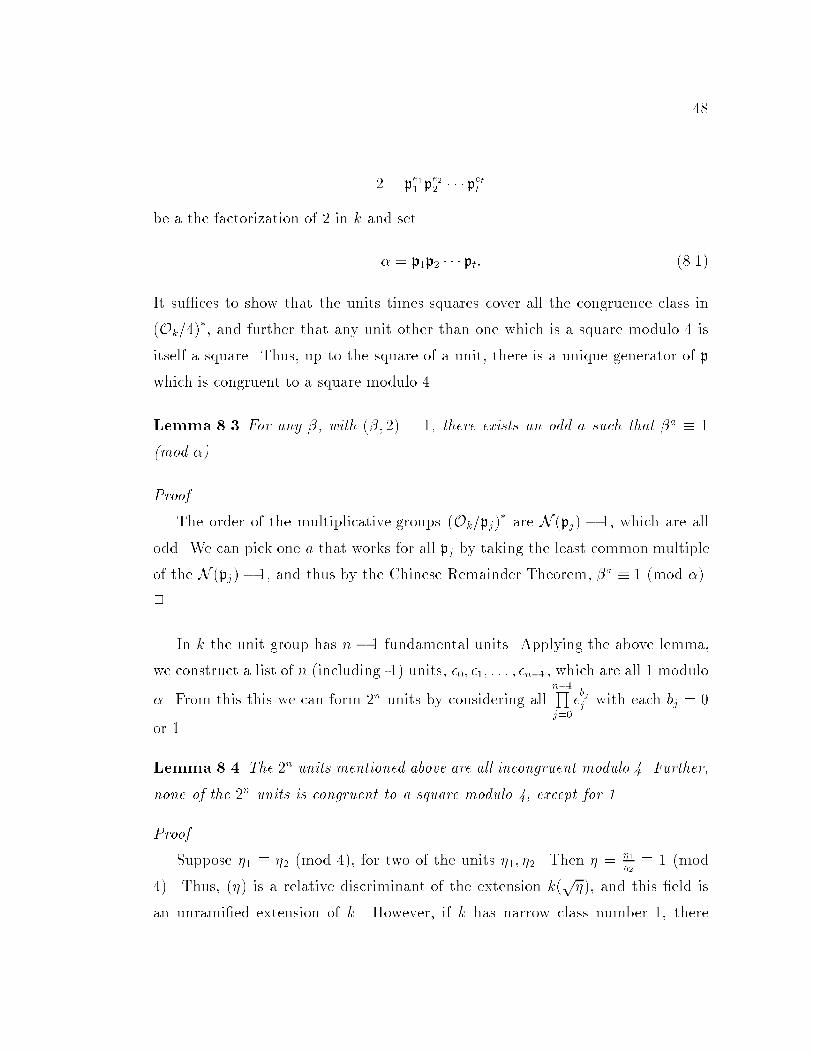
48

2 = pe11 pe22 � � � pett

be a the factorization of 2 in k and set

� = p1p2 � � � pt: (8.1)

It su�ces to show that the units times squares cover all the congruence class in

(Ok=4)�, and further that any unit other than one which is a square modulo 4 is

itself a square. Thus, up to the square of a unit, there is a unique generator of p

which is congruent to a square modulo 4.

Lemma 8.3 For any �, with (�; 2) = 1, there exists an odd a such that �a � 1

(mod �).

Proof.

The order of the multiplicative groups (Ok=pj)� are N (pj) � 1, which are all

odd. We can pick one a that works for all pj by taking the least common multiple

of the N (pj)� 1, and thus by the Chinese Remainder Theorem, �a � 1 (mod �).

2

In k the unit group has n � 1 fundamental units. Applying the above lemma,

we construct a list of n (including -1) units, �0; �1; : : : ; �n�1, which are all 1 modulo

�. From this this we can form 2n units by considering alln�1Qj=0

�bjj with each bj = 0

or 1.

Lemma 8.4 The 2n units mentioned above are all incongruent modulo 4. Further,

none of the 2n units is congruent to a square modulo 4, except for 1.

Proof.

Suppose �1 � �2 (mod 4), for two of the units �1; �2. Then � = �1�2� 1 (mod

4). Thus, (�) is a relative discriminant of the extension k(p�), and this �eld is

an unrami�ed extension of k. However, if k has narrow class number 1, there

49

are no unrami�ed extensions, yielding a contradiction. Additionally, all of the 2n

units are not squares, since they are products of odd powers of fundamental units.

Therefore, if �j � � (mod 4), k(p�j) would also be an unrami�ed extension, which

is impossible. 2

Here is the �rst indication of why the assumption of narrow class number one is

necessary; with wide class number 1 only, there are rami�ed extensions at in�nite

primes, so negative units could be congruent to squares, and there will not be 2n

incongruent units modulo 4. Also, we need that k is totally real or there would

again be a shortage of units.

Lemma 8.5 Let � be as in (8.1). There are 2n

N (�)congruence classes of numbers

� modulo 4 in Ok such that � � x2 (mod 4) and � � 1 (mod �).

Proof.

By the Chinese Remainder Theorem, � � 1 (mod �) if and only if � � 1

(mod pj) for all j. If we can show there are N (pe�1j ) such � (mod pej) which are

congruent to 1 (mod pj), the Chinese Remainder Theorem will give us the desired

result. This is because 2n

N (�)= N ( 2

�) =

Qj

N (pej�1j ). We thus consider each pj

separately.

Suppose we have two numbers x and x� such that x2 � (x�)2 (mod p2ejj ). This

is the case if and only if x � x� (mod pejj ), since x� x� � x+ x� (mod �

ejj ). We

therefore need only consider x modulo pej. Express x = x0 + x1pj + x2p2j + � � � +

xe�1pe�1j , where the xi are chosen from a �xed set of N (pj) residues modulo pj . If

x2 � 1 (mod pej), then x20 � 1 (mod pj), and since (Ok=pj)� is a group of odd order

there is only 1 square root modulo p. Thus x0 is determined, and there are then

N (pe�1j ) (from the choices of xi i = 1 : : : e� 1) incongruent values of x2 (mod p2ej )

that are 1 (mod pej), as desired. 2

50

Proof of Theorem 8.2.

We have by Lemma 8.3 there is an even b with ��b � 1 (mod �). Lemma 8.4

gives 2n units that are 1 (mod �) that are not congruent to each other or to squares

modulo 4. By Lemma 8.5, there are 2n

N (�)elements which are squares modulo 4

which are 1 modulo �. Since 1 is the only one of the 2n units which is a square, the

units times squares cover all 4n

N (�)congruence classes modulo 4 that are 1 modulo

�. Thus there is a unique � and t such that ��b � �t2 (mod 4), and the � in

Theorem 8.2 is exactly the generator of p which satis�es the congruence

� � �s2 (mod 4):

2

This proof then gives us an explicit construction of � for primes of odd norm.

The di�culty is determining the prime discriminants associated to primes dividing

2. For any real narrow class number 1 K, the construction of these prime discrim-

inants must be possible. However, since this paper has been concentrating on real

quadratic �elds, this is where we direct our attention.

8.2 Narrow class number one quadratic �elds

The possible even prime discriminants will depend on how 2 factors in the �eld.

There are three cases which arise in narrow class number one real quadratic �elds: 2

splits in k, 2 is prime in k, and k = Q(p2). The methodology of the construction is

essentially the same in all cases. For this reason, we provide a detailed construction

only in the case where 2 is prime in k, as this is the situation in our recurring

example k = Q(p5). Having done so, we will also give a constructive proof of

Theorem 8.1 in this case.

Let k be a real quadratic �eld, such that (2) is a prime ideal in k, and let �0 be

the fundamental unit. When � is square free, the only possible �eld discriminants

of k(p�) are � and 4�. By Lemma 8.4, there are 4 incongruent units modulo

51

4 which are 1 modulo 2, which we denote f1;�1; �;��g, where � = �0 or � = �30.

According to lemma 8.5, 1 is the only square modulo 4 which is 1 modulo 2.

For primes p of odd norm, Theorem 8.2 gives a unique generator �p of p which

is a relative �eld discriminant. For primes dividing 2, there are only two possible

discriminants when considered as ideals: (4) and (8). A discriminant of (4) corre-

sponds to k(p�), � a unit, and (8) corresponds to k(

p2�). The seven possibilities

listed in Table 8.1 yield seven di�erent numerical discriminants, each corresponding

to a di�erent quadratic extension.

discriminant integral basis

�p, �p � s2 (mod 4) [1;s+p�p

2]

-4 [1;p�1]

�4� [1;p��]

4� [1;p�]

8 [1;p2]

-8 [1;p�2]

8� [1;p2�]

�8� [1;p�2�]

Table 8.1: Prime Discriminants when 2 is prime in k

Theorem 8.6 Let k be a real quadratic �eld of narrow class number one in which

2 is prime. Given � the relative �eld discriminant of k(p�), � square-free, we can

factor � uniquely up to squares of units as the product of the prime discriminants

given in Table 8.1.

Before we begin the proof, we will �nd the following two results useful.

Proposition 8.7 (Eisenstein Criterion)

Let f(x) = xn+ an�1xn�1+ � � �+ a1x+ a0 be a polynomial with Ok coe�cients. If

there exists a prime ideal p 2 Ok such that pjai for all i = 1; 2; : : : ; n, but p2 6 ja0,

52

then the polynomial f(x) is irreducible in Ok[x]. Furthermore if � is a root of f(x),

then the power of p in the �eld discriminant of k(�) is the same as the power of p

in the polynomial discriminant of f(x).

Proposition 8.8 (Almost Eisenstein Criterion)

Let f(x) = xn + an�1xn�1 + � � � + a1x + a0 be an irreducible polynomial with Okcoe�cients. Let p of Ok, such that p divides the polynomial discriminant of f(x),

and further pjai for all i = 1; 2; : : : ; n, and p2ja0. Then if � is a root of f(x), the

factor of p in the �eld discriminant of k(�) is lower than the power of p in the

polynomial discriminant of f(x) by at least p2.

Proof of Theorem 8.6.

We will �rst show that one can factor a discriminant into prime discriminants

from the table. One can factor �

� = �2n0 � 2aY

�p = �2n0 � 2a ��;

where n 2Z, a 2 f0; 2; 3g, and � 2 f1;�1; �;��g.If a is even, there are no factors of 2 in �, and the �eld is generated by the

polynomial x2����. The polynomial arrived at by making the change of variables

x! x+ 1 generates the same �eld, and

x2 + 2x+ (1� ���);

has discriminant 4���. If � = 1, then this polynomial is almost Eisenstein with

respect to 2, since the �p are all 1 modulo 4. The �eld discriminant then has no

factor of 2, by proposition 8.8, and a = 0. If � is any of the other 3 units, the

polynomial is Eisenstein with respect to 2 and by proposition 8.7 a = 2. Since �4,4�, �4� all appear, the factorization is complete.

If a = 3, the �eld is generated by the polynomial x2�2���, which is Eisensteinwith respect to 2, independent of the value of �. The list of prime discriminants

has 8� for each value of �, and the factorization is complete.

53

The last detail that needs to be veri�ed is that the factorizations given above are

unique. We have shown that the factorization of the odd part of the discriminant

is unique. The only concern, therefore, is that one could generate one of the even

discriminants from a product of some others. However, although it is true that, for

example, k(p(8)(�4�)) generates the same �eld as k(

p�8�), the goal is to factorthe discriminant uniquely up to the square of a unit. The discriminant of k(

p�8�)is �8�, and �8� 6= (8)(�4�)�2n0 . The entire list from table 8.1 is thus necessary,

and the factorizations are unique.

2

We now give the list of the prime discriminants in the two remaining cases.

Although we shall not go through the details, the last proof gives the idea of how

this could be done.

In the case where (2) = �2�0

2, we take �2 � 1 (mod �022 ) and �

0

2 � 1 (mod �22).

Further, let � = ��0 so that � � 1 (mod �022 ) and � � �1 (mod �22). The only

square modulo 4 is 1.

In the case k = Q(p2), 2 = �22; �0 = 1 + �2. There are now 2 squares modulo

4 which are 1 modulo �2, they are 1 and 3 + 2�2.

Example.

Consider again k = Q(p5) and K = k(

p�17 � 4!) of discriminant �K = �68 �16!, where (�K) = (4)p11p31. The ideal p11 is generated by �11 = 1 � 3!. This

is not 1 modulo 2, so we consider �311 = 1 � 36! � 1 (mod 4), so �11 is the

prime discriminant. The primep31 = �31 = 2 � 5!, which also is not 1 modulo

2, but �331 = 33 � 160! is, and �31 is a prime discriminant. One checks that

�K=(pi11�31) = �4. So the factorization of �K into prime discriminants is given by

�K = �4 � �11 � �31:

54

discriminant integral basis

�p, �p � 1 (mod 4) [1;1+

p�p

2]

�32 [1;1+

p�2

�0

2

]

��32 [1;1+

p��2

�0

2

]

�032 [1;

1+p�0

2

�2]

���032 [1;1+p���02

�2]

��22 [1; 1+p�

�0

2

]

���022 [1; 1+p���2

]

Table 8.2: Prime Discriminants when 2 splits in k

discriminant integral basis

�p, �p � s2 (mod 4) [1;s+p�p

2]

-2 [1;p�1�2

]

�4� [1;p��]

4� [1;p�]

4�2 [1;p�2]

�4�2 [1;p��2]

4��2 [1;p��2]

�4��2 [1;p���2]

Table 8.3: Prime Discriminants in Q(p2).

55

8.3 Narrow class number 2 quadratic �elds

When the narrow class number is not 1, we no longer have enough units to cover

all classes modulo 4. There may now be a unit other than 1 which is congruent to

a square modulo 4 because there are now unrami�ed extensions at in�nite primes.

This means that for some prime ideals, there is no relative discriminant which is

divisible by only that prime ideal.

As an example, consider the �eld Q(p3), in which 59 = p59p

059. There is no

generator of p59 that is a relative �eld discriminant. The smallest discriminant

involving p59 is 2p59.

In light of the above observation, one can no longer hope to factor discriminants

uniquely up to squares of units into prime discriminants. The best one could hope

for is to factor discriminants uniquely up to a square factor of primes dividing two.

While preliminary investigations indicate that this is possible, the proof is rather

tedious and the usefulness that prime discriminants serve in the next chapter will

not be directly applicable. To give a thorough examination of this situation would

stray from the themes of this paper, and is mentioned as a possible future research

subject of interest.

Chapter 9

Genus Theory

Gauss in his study of the class group of forms in [7] developed the notion of

genus theory. In essence, he was able to categorize the 2-Sylow subgroup of the

class group. This is essentially done by forming quadratic characters associated

with prime discriminants, and categorizing forms according to the value they take

on these characters. One of the fascinating consequences of this is the following

theorem.

Theorem 9.1 (Gauss) Let d be the discriminant of k, a complex quadratic �eld,

and let d have exactly t prime factors. Then the class number h(k) is divisible by

a factor of 2t�1.

To prove an analogous theorem will be our �rst goal. We will do so, however,

from the standpoint of ideals rather than forms. Once this is established, we

will look at how this connects with quadratic forms. The proofs will be taking

advantage of more sophisticated algebraic number theory machinery than has been

previously necessary, and the reader is directed to [10] for details on these tools,

and [1], [7], [9] for treatment of genus theory of quadratic �elds.

56

57

9.1 The genus �eld

Let k be a real quadratic �eld of narrow class number 1, and let K be a totally

complex quadratic extension of k. Also let L be the Hilbert class �eld of K,

G =Gal(L=k), and H =Gal(L=K). There is an isomorphism between H and the

ideal class group of K which identi�es any � 2 H with the class of a prime ideal

P having � as its Frobenius automorphism.

Lemma 9.2 Let � be an element of G that is not an element of H. Then � 2 = 1.

If � is any element of H, then �� = ���1.

Proof.

Note that for K totally complex, there will always be such a � , namely complex

conjugation. We �x a primeP of L (which divides p in k), such thatP is unrami�ed

in L=k, and � = �(P; L=k), the Frobenius automorphism of P with respect to L=k.

If p splits in K, then h� i = GD(P; L=k) � H, which is a contradiction. Therefore

p is prime in K.

Since � = �(P; L=K),

�N (p) � � (�) (mod P);

and therefore

�N (p2) � � 2(�) (mod P):

Now since p is prime in K, NK=Q(p) = Nk=Q(p2), and �(P; L=K) = � 2. Further-

more, since � 2 = �(P; L=K), � 2 2 H, and using the class �eld isomorphism, � 2

must be the identity element of H, since it corresponds to the ideal p, which is

principal.

For the second part of the proof, choose a prime p in k such that p = P �P in

K, with �(P;H=K) = �. We have that �( �P; L=K) = �(� (P); L=K) = ��1�� .

Since P �P = p is principal, the product of their Frobenius automorphisms is the

58

identity. So recalling that � 2 = 1 implies � = ��1,

(�)(��� ) = 1

�� = ���1:

2

The group G might be thought of as \almost dihedral," since it has the same

relations as a dihedral group except that H is not necessarily cyclic.

De�nition The genus �eld of K with respect to k is the maximal abelian extension

of k contained in the Hilbert Class �eld of K.

Theorem 9.3 Let F be the genus �eld of K with respect to k. Then Gal(F=k) is

an elementary abelian 2 group.

Proof.

All of the relevant �elds are shown in Figure 9.1. Since F is the maximal

abelian extension of k contained in L, G1 is the minimal normal subgroup of G

such that G=G1�= Gal(F=k) is abelian. Consider the natural homomorphism

from G to G=G1, and denote the image of an element g 2 G by bg. Let � be an

element of H, and � be an element of G which is not in H. Since the group G=G1

is abelian, b�b� = b�b�. Also by Lemma 9.2,

[(��1) = \(��� )

= \(��� )

= b�:Therefore,

b�2 = b1:Thus every element of G=G1 is of order 2, completing the proof. 2

59

L

G1

F H

G

K

k

Figure 9.1: Genus �eld tower

De�nition The principal genus is the subgroup of the of the class group corre-

sponding to the genus �eld.

This corresponds to the group G1 in the last theorem and in Figure 9.1. As

stated in the proof of the theorem, the principal genus is also the minimal subgroup

of the class group such that the quotient is abelian.

Proposition 9.4 The principal genus is the subgroup of the class group consisting

of the squares.

Proof.

Let G1 be the principal genus, and S = fs2 j s 2 Hg. Since every element of

H=G1 is of order 2, in the projection H ! H=G1, S is mapped to the identity, so

S � G1.

60

Further, S is normal in H as

(xsx�1)2 = (xsx�1)(xsx�1)

so that the conjugate of a square is a square. Since every element of H=S has order

2, H=S is abelian. By the minimality of the principal genus, G1 � S, and we are

done. 2

We have demonstrated that for K = k(p�K), with �K the relative discriminant

of K=k, one can factor � uniquely into a product of prime discriminants,

� =

tYj=1

�pj : (9.1)

The aim now is to prove the following theorem.

Theorem 9.5 The genus �eld of K is the composite of the quadratic �elds Kj =

k(p�pj), where the �pj are as in equation (9.1).

Proof.

Let Kn = k(p�n) be a quadratic extension of K, where �n is the discriminant

relative to k. Kn is contained in F if and only ifM = K(p�n) is unrami�ed overK.

This is the case exactly when the relative discriminant of M over K, �M=K = (1).

To calculate the discriminant �M=K, notice that M is a degree 4 extension of k

with three intermediate �elds: K;Kn, K0

n = k(p��n) of discriminant �n0 . We will

show that Kn is contained in F if and only if � = �n�n0 , with (�n; �n0 ) = 1.

By the conductor discriminant formula, the discriminant of M relative to k,

�M , is given by

(�M ) = (��n�n0 ): (9.2)

There is also another classical formula for computing �M given by

(�M) = NK=k(�M=K)(�[K:k]

K ): (9.3)

61

Let

�n =

tnYj=1

�pj

snYj=1

��pj;

where we have suitably ordered the �pj in 9.1, and the ��pj are prime discriminants

not dividing �. Notice

��n =

tnYj=1

�2pj

tYj=tn+1

�pj

snYj=1

��pj ;

and hence it follows that

�n0 =

tYj=tn+1

�pj

snYj=1

��pj :

We then have by (9.2)

(�M) = (�2)(

snYj=1

��pj)2:

If Kn � F , we have �M=K = (1), so comparing (9.2) and (9.3) we see that

(�)2(

snYj=1

��pj)2 = (�)2

so that there are no primes ��pj in the factorization of �n. Thus �nj�, and �n0 = ��n,

and they are obviously relatively prime. If conversely, � = �n�n0 , again comparing

equations (9.2) and (9.3) leads to

(�)2 = NK=k(�M=K)(�)2;

so thatM is unrami�ed overK, and Kn � F . We then have that F = k(fp�ng) =k(p�p1;p�p2; : : : ;

p�pt). 2

The next result is an immediate corollary.

Corollary 9.6 Let k be a real quadratic �eld of narrow class number 1, and K be

a totally complex extension of k. If the relative discriminant of K can be factored

into t prime discriminants, then there is a factor of 2t�1 in the class number of K.

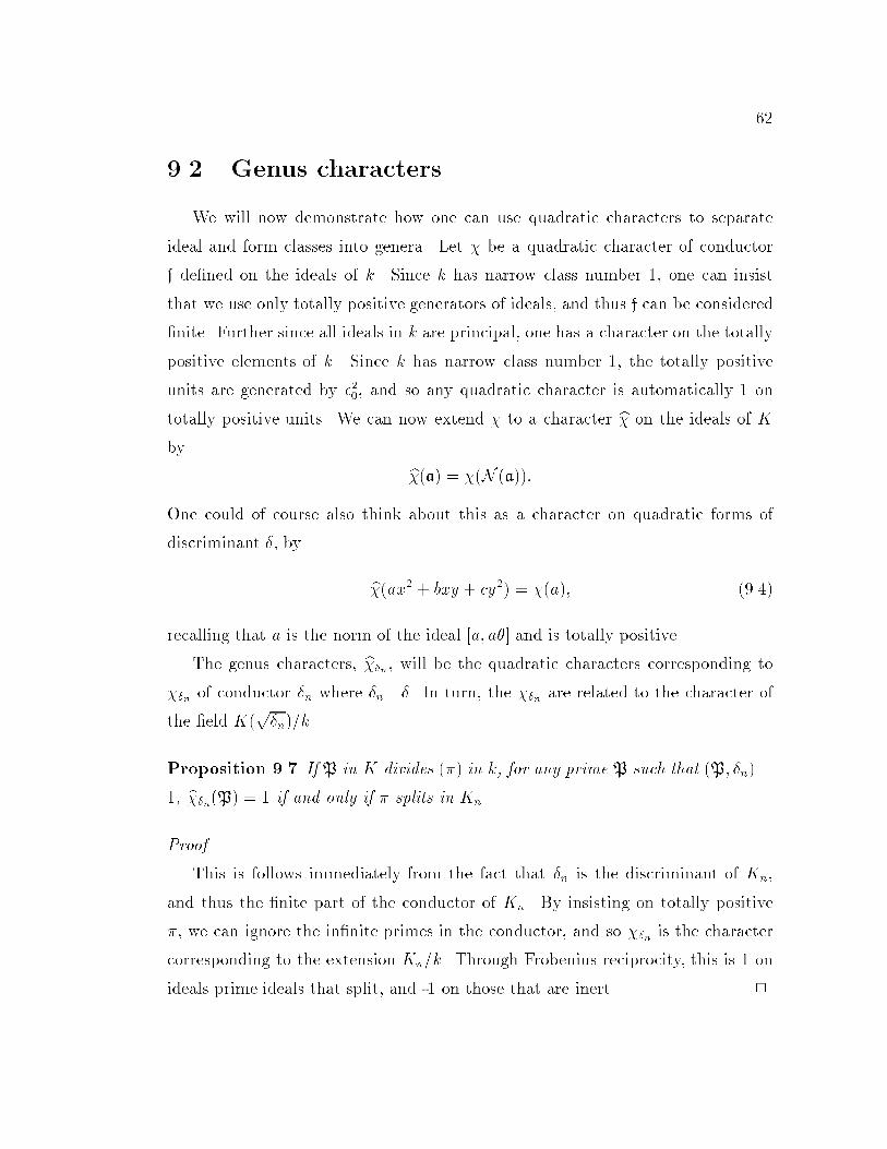
62

9.2 Genus characters

We will now demonstrate how one can use quadratic characters to separate

ideal and form classes into genera. Let � be a quadratic character of conductor

f de�ned on the ideals of k. Since k has narrow class number 1, one can insist

that we use only totally positive generators of ideals, and thus f can be considered

�nite. Further since all ideals in k are principal, one has a character on the totally

positive elements of k. Since k has narrow class number 1, the totally positive

units are generated by �20, and so any quadratic character is automatically 1 on

totally positive units. We can now extend � to a character b� on the ideals of K

by

b�(a) = �(N (a)):

One could of course also think about this as a character on quadratic forms of

discriminant �, by

b�(ax2 + bxy + cy2) = �(a); (9.4)

recalling that a is the norm of the ideal [a; a�] and is totally positive.

The genus characters, b��n, will be the quadratic characters corresponding to

��n of conductor �n where �n j �. In turn, the ��n are related to the character of

the �eld K(p�n)=k.

Proposition 9.7 If P in K divides (�) in k, for any prime P such that (P; �n) =

1, b��n(P) = 1 if and only if � splits in Kn.

Proof.

This is follows immediately from the fact that �n is the discriminant of Kn,

and thus the �nite part of the conductor of Kn. By insisting on totally positive

�, we can ignore the in�nite primes in the conductor, and so ��n is the character

corresponding to the extension Kn=k. Through Frobenius reciprocity, this is 1 on

ideals prime ideals that split, and -1 on those that are inert. 2

63

In fact one has that in any class �eld extension, the primes that split com-

pletely are exactly those primes p such that every character evaluated at p is 1.

In particular, the primes that split completely in the Hilbert class �eld are the

principal prime ideals. Since the genus �eld is contained in the Hilbert class �eld,

we have that the principal prime ideals split completely in it as well, and so all the

genus characters are one on principal ideals. Thus our genus characters are well

de�ned on ideal classes, and so are actually characters of the class group.

Proposition 9.8 If � = �1�2, with (�1; �2) = 1, then b��1 = b��2.Proof.

Since (�1; �2) = 1, one can factor b�� = b��1b��2. If P is inert in K, N (P) = (�2),

b��1(P) = b��2(P) = 1. If � splits in Kn, b��(P) = 1, and b��1(P) = b��2(P). 2

We can utilize this relationship to now de�ne b��(P) for all P, including those

Pj�. If Pj�1, then we de�ne b��(P) = b��2(P).

We conclude with an examination of how to explicitly de�ne the genus charac-

ters. For �p not dividing two, since (Ok=�p)� is cyclic, it must be the case that

b��p(a) = N (a)N (�p)�1

2 (mod �p):

Note that this is exactly how the characters associated to odd primes are de�ned

in the classical case. However, the characters corresponding to even prime discrim-

inants are not so simple, and depend on the structure of (Ok=(�p))�.In the case where 2 is prime in k, one can verify that

(Ok=4)� �=Z=3Z�Z=2Z�Z=2Z;

and

(Ok=8)� �=Z=3Z�Z=2Z�Z=2Z�Z=4Z:

Further, (Ok=4)� is generated by �0 and �1, where �60 � 1 (mod 4). One can see

this by recalling that �0 and �1 are not squares modulo 4. The characters modulo

64

4 are thus determined by their values at �0 and �1. To determine which �eld

correspond to which characters, we consider the in�nite primes, and the fact that

the character associated to a �eld is 1 on units.

The �eld K = k(p�4) is totally complex, both in�nite primes are present in

the conductor. Since �1 is totally negative also, we must have that ��4(�1) = 1.

Since �0 is not totally positive, we need ��4(�0) = �1. ForK = k(p�4�0), only the

in�nite prime associated to k is present. Since �0 > 0 and �1 < 0, ��4�0(�1) = �1,and ��4�0(�0) = 1. ForK = k(

p4�0), the in�nite prime associated to k0 is present in

the conductor. Since �00 < 0;�1 < 0, we require �4�0(�1) = �1, and �4�0(�0) = �1.

For the characters modulo 8, the characters are determined by their values on

�1; �0; and 1 + 4�0. The order of �0 is either 4 or 12 and not 3 or 6 because if it

were, (�30� 1)(�30 + 1) � 0 (mod 8). Therefore, 4j(�30 � 1) or (�30+ 1), and ��0 � s2(mod 4), for some s. For the characters to be primitive, they must be -1 at 1+4�0,

or else we have one of the characters modulo 4.

For K = k(p8), there are no in�nite primes in the conductor and �8(�1) = 1,

and �8(�0) = 1. For K = k(p�8), both in�nite primes are in the conductor and

we have ��8(�1) = 1, and ��8(�0) = �1. In the case K = k(p8�0) we need

consider the in�nite prime associated to k, and therefore �8�0(�1) = �1, and�8�0(�0) = 1. Finally for K = k(

p�8�0) the in�nite prime associated to k0 is

present, so ��8�0(�1) = �1, and ��8(�0) = �1.In the case where (2) = �2�

02, we take �2 � 1 (mod �02

2), and �02 � 1 (mod �22).

Further, we take � = ��0 such that � � 1 (mod �022). One can establish the genus

characters as follows.

There will be one character arising from (Ok=�22)� �= (Z=4Z)�. Further the

�eld, K = k(p��22) has the in�nite prime of k0 in the conductor. Since � � �1

(mod �22), the character associated to ��22 is the only character possible where

�(�1) = �1. We have a similar result for the conjugate case, which has the in�nite

prime associated to k in the conductor, and � � 1(mod �02). Again �(�1) = �1,and the character of the �eld is 1 on all units.

There will also be 2 characters arising from (Ok=�32)� �= (Z=8Z)�. One of the

65

primitive characters is 1 at 1 and -1, the other is 1 at 1 and 3. Notice that one of

��32 and �32 has both conjugates with the same parity, and the other has conjugates

with opposite parity, so we pick �2 such that it has positive norm. In this way

��32(�1) = 1, to satisfy the congruence of the in�nite prime. In the other case,

to satisfy the congruence of the in�nite prime, we have ���32 (�1) = �1. A similar

argument will give the characters associated to �02.

We note an interesting congruence that arises out of this theory. If we choose

�2 to have positive norm, then the congruence class of � modulo �32 depends on

the sign of �2. We have that � � �1 (mod �22), so � � �1 (mod �32) or � � 3 (mod

�32). If �2 < 0, then both in�nite primes appear in the conductor of k(p�32), so we

must have ��32(�) = �1. Therefore, � � 3 (mod �32). If on the other hand �2 > 0,

there are no in�nite primes in the conductor of k(p�32), and ��32 (�) = 1. In this

case then, � � �1 (mod �32). Naturally there is a similar congruence modulo �023.

(a;b; c) b��4 b��11 b��31(1; 0; 17 + 4!) 1 1 1

(5;�4 + 4!; 5) 1 1 1

(2 + !;�2� 2!; 10 � !) 1 -1 -1

(2 + !; 2 + 2!; 10 � !) 1 -1 -1

(5 � !;�2; 4 + 2!) -1 1 -1

(5� !; 2; 4 + 2!) -1 1 -1

(4� !; 0; 5 + 3!) -1 -1 1

(2; 2; 9 + 2!) -1 -1 1

Table 9.1: Genera of forms for Q(p5)(p�68� 16!)

Example.

Recall our recurring example where k = Q(p5), and K = �68� 16!. We saw

that this factors into prime discriminants as

68 � 16! = (�4)(1 � 3!)(2 � 5!):

66

Corollary 9.6 predicts that there should be a factor of 4 in the class number of K,

and we saw that in fact the class number was 8. This means that each of the four

genera contain 2 ideal classes. The 3 genus characters are b�p11; b�p31

; and b��4. Thecharacter ��4 is given by

��4(a) =

8<:

1 N (a) � �(�2)c (mod 4)

�1 otherwise.

and ��11 and ��31 are given in (9.2). Using equation (9.4), we calculate the four

genera for the class group in terms of forms. The results are given in Table 9.1.

Bibliography

[1] Duncan Buell, Binary quadratic forms : Classical theory and modern compu-

tations, Springer-Verlag, 1989.

[2] G. Claus, Die Randmannigfaltigkeiten und die `tiefsten' Punkt des Fundamen-

talbereichs f�ur drei Hilbertsche Modulgruppen., Math. Annalen 176 (1968),225{256.

[3] Henri Cohen, A course in computational algebraic number theory, Springer-

Verlag, 1993.

[4] Harvey Cohn, A numerical survey of the oors of various hilbert fundamental

domains, Math. Comp. 19 (1965), 594{605.

[5] , Note on how hilbert modular domains become increasingly compli-

cated, J. Math. Anal. Appl. 15 (1966), 55{59.

[6] Daberkow, Fieker, Kl�uners, Pohst, Roegner, and Wildanger, KANT V4, J.Symbolic Comp. 24 (1997), 267{283.

[7] Carl Friedrich Gauss, Disquisitiones arithmeticae, Springer-Verlag, 1986,

translated by Arthur A. Clarke.

[8] L.J. Goldstein, On prime discriminants, Nagoya Math. J. 45 (1971), 119{127.

[9] Erich Hecke, Lectures on the Theory of Algebraic Numbers, Springer-Verlag,

1981, translated by George U. Brauer and Jay R. Goldman with the assistanceof R. Kotzen.

[10] Wladyslaw Narkiewicz, Elementary and Analytic Theory of Algebraic Num-

bers, 2nd ed., Springer-Verlag, 1990.

[11] H. M. Stark, Modular forms and related objects, Canadian Mathematical So-

ciety Conference Proceedings, vol. 7 (Providence, R.I.), Amer. Math. Soc.,1987, pp. 421{455.

67

68

[12] , Galois theory, algebraic number theory, and zeta functions, From

Number Theory to Physics, ch. 6 (M. Waldschmidt, et. al., ed.), Springer-

Verlag, 1992, pp. 313{393.