
QSAR and pharmacophore modelingfch.upol.cz/wp-content/uploads/2015/11/QSAR... · QSAR and...
64
QSAR and pharmacophore modeling Pavel Polishchuk, Ph.D. Karel Berka , Ph.D. Jindřich Fanfrlík , Ph.D. Martin Lepšík , Ph.D. Institute of Molecular and Translational Medicine Palacky University [email protected] Advanced in silico drug design workshop Palacky Univrsity, Olomouc, Czech Republic 30 January – 1 February 2017
Transcript of QSAR and pharmacophore modelingfch.upol.cz/wp-content/uploads/2015/11/QSAR... · QSAR and...
QSAR and pharmacophore modeling
Pavel Polishchuk, Ph.D.Karel Berka , Ph.D.
Jindřich Fanfrlík , Ph.D.Martin Lepšík , Ph.D.
Institute of Molecular and Translational MedicinePalacky University
Advanced in silico drug design workshopPalacky Univrsity, Olomouc, Czech Republic 30 January – 1 February 2017
Quantitative structure-activity relationship (QSAR) modeling
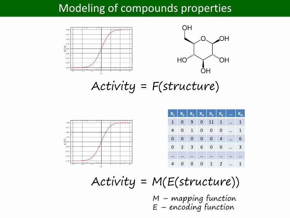
Activity = F(structure)
M – mapping functionE – encoding function
Modeling of compounds properties
Activity = M(E(structure))
X1 X2 X3 X4 X5 X6 … XN
1 0 9 0 11 1 … 1
4 0 1 0 0 0 … 1
0 0 0 0 0 4 … 6
0 2 3 6 0 0 … 3
… … … … … … … …
4 0 0 0 1 2 … 1
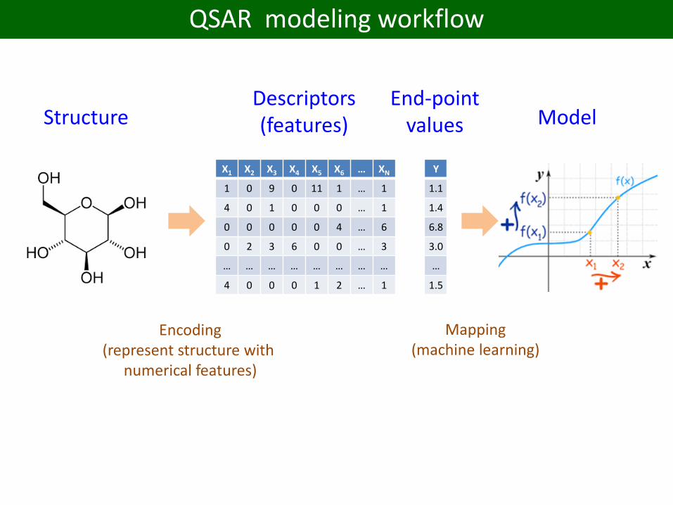
QSAR modeling workflow
X1 X2 X3 X4 X5 X6 … XN
1 0 9 0 11 1 … 1
4 0 1 0 0 0 … 1
0 0 0 0 0 4 … 6
0 2 3 6 0 0 … 3
… … … … … … … …
4 0 0 0 1 2 … 1
StructureDescriptors(features) Model
Encoding(represent structure with
numerical features)
Mapping(machine learning)
Y
1.1
1.4
6.8
3.0
…
1.5
End-pointvalues

Overall QSAR workflow
Input data
Bioassays
Databases
PreprocessingFeature
engineeringModel
learningModel
validation
Classification
Regression
Clustering
Cross-validation
Bootstrap
Test set
Applicability Domain
Feature selection
Feature combination
Data normalization
Feature extraction
Interpretation
j
j
i
i
z
xxx
'
Step 1. Data collection
Scientific literature and patentsDatabases (ChEMBL, PubChem, BindingDB, etc)Own experimental data
Traditionally modeled compounds should have the same mechanism of action, however using of complex non-linear machine learning method allows to model data sets with mixed or even unknown mechanism of action with reasonable accuracy.
Conditions may substantially influence the results of bioassays (change in temperature, activators, detectors, etc)
Units checking

Each found error is next to last
Step 2. Data curation (normalization)
strange units
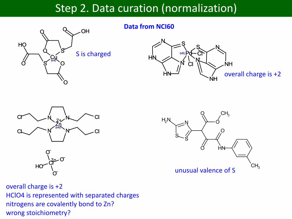
Step 2. Data curation (normalization)
Data from NCI60
S is charged
overall charge is +2
overall charge is +2HClO4 is represented with separated chargesnitrogens are covalently bond to Zn?wrong stoichiometry?
unusual valence of S
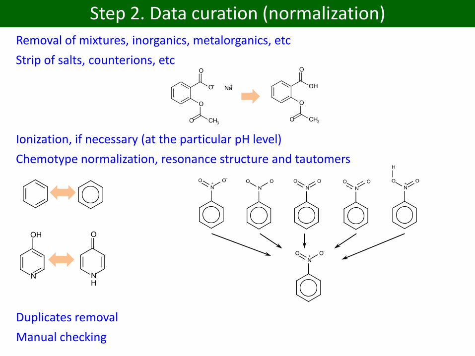
Step 2. Data curation (normalization)
Removal of mixtures, inorganics, metalorganics, etc
Strip of salts, counterions, etc
Ionization, if necessary (at the particular pH level)
Chemotype normalization, resonance structure and tautomers
Duplicates removal
Manual checking
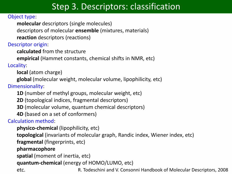
Step 3. Descriptors: classificationObject type:
molecular descriptors (single molecules)descriptors of molecular ensemble (mixtures, materials)reaction descriptors (reactions)
Descriptor origin:calculated from the structureempirical (Hammet constants, chemical shifts in NMR, etc)
Locality:local (atom charge)global (molecular weight, molecular volume, lipophilicity, etc)
Dimensionality:1D (number of methyl groups, molecular weight, etc)2D (topological indices, fragmental descriptors)3D (molecular volume, quantum chemical descriptors)4D (based on a set of conformers)
Calculation method:physico-chemical (lipophilicity, etc)topological (invariants of molecular graph, Randic index, Wiener index, etc)fragmental (fingerprints, etc)pharmacophorespatial (moment of inertia, etc)quantum-chemical (energy of HOMO/LUMO, etc)etc. R. Todeschini and V. Consonni Handbook of Molecular Descriptors, 2008
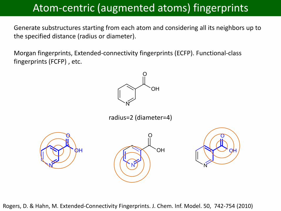
Atom-centric (augmented atoms) fingerprints
Generate substructures starting from each atom and considering all its neighbors up to the specified distance (radius or diameter).
Morgan fingerprints, Extended-connectivity fingerprints (ECFP). Functional-class fingerprints (FCFP) , etc.
radius=2 (diameter=4)
Rogers, D. & Hahn, M. Extended-Connectivity Fingerprints. J. Chem. Inf. Model. 50, 742-754 (2010)
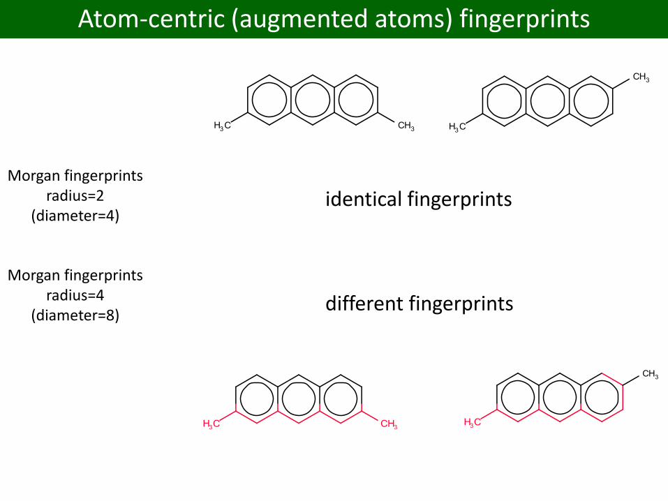
Morgan fingerprintsradius=2
(diameter=4)
Morgan fingerprintsradius=4
(diameter=8)
identical fingerprints
different fingerprints
Atom-centric (augmented atoms) fingerprints
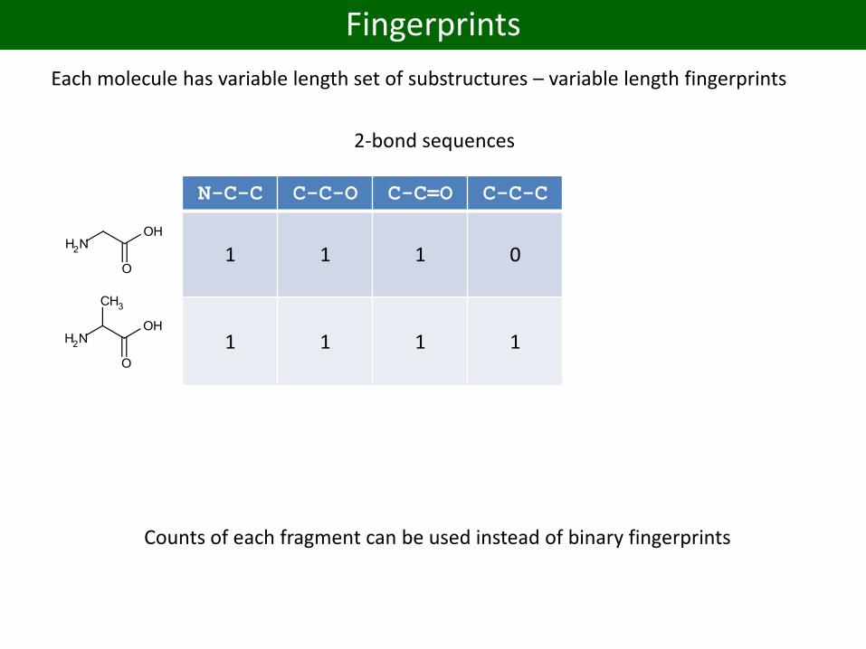
Fingerprints
Each molecule has variable length set of substructures – variable length fingerprints
N-C-C C-C-O C-C=O C-C-C C:C:C C:C:N C:N:C
1 1 1 0 0 0 0
1 1 1 1 0 0 0
0 0 0 0 1 1 1
2-bond sequences
Counts of each fragment can be used instead of binary fingerprints
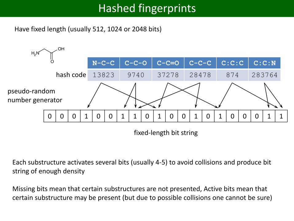
Hashed fingerprints
Have fixed length (usually 512, 1024 or 2048 bits)
hash code
N-C-C C-C-O C-C=O C-C-C C:C:C C:C:N
13823 9740 37278 28478 874 283764
0 0 0 1 0 0 1 1 0 1 0 0 1 0 1 0 0 0 1 1
pseudo-randomnumber generator
fixed-length bit string
Each substructure activates several bits (usually 4-5) to avoid collisions and produce bit string of enough density
Missing bits mean that certain substructures are not presented, Active bits mean that certain substructure may be present (but due to possible collisions one cannot be sure)
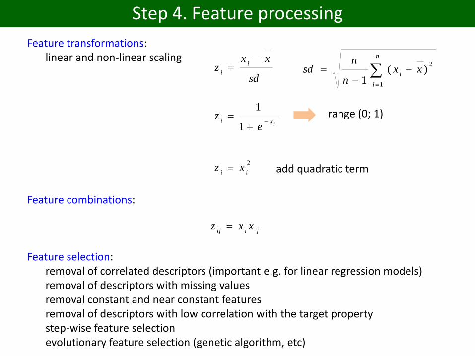
Step 4. Feature processing
Feature transformations:linear and non-linear scaling
Feature combinations:
Feature selection:removal of correlated descriptors (important e.g. for linear regression models)removal of descriptors with missing valuesremoval constant and near constant featuresremoval of descriptors with low correlation with the target propertystep-wise feature selectionevolutionary feature selection (genetic algorithm, etc)
sd
xxz
i
i
n
i
ixx
n
nsd
1
2)(
1
ixi
ez
1
1range (0; 1)
jiijxxz
2
iixz add quadratic term
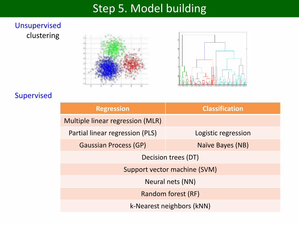
Step 5. Model building
Unsupervisedclustering
Supervised
Regression Classification
Multiple linear regression (MLR)
Partial linear regression (PLS) Logistic regression
Gaussian Process (GP) Naïve Bayes (NB)
Decision trees (DT)
Support vector machine (SVM)
Neural nets (NN)
Random forest (RF)
k-Nearest neighbors (kNN)
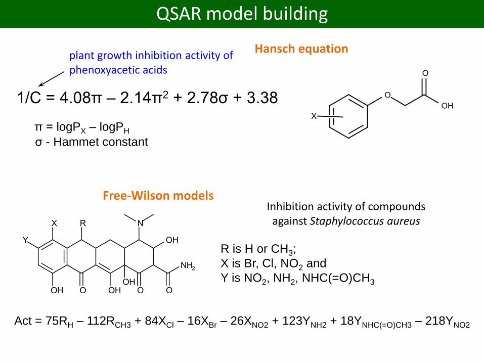
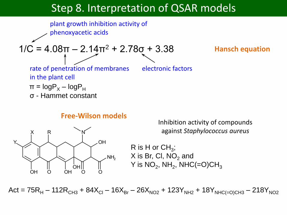
1/C = 4.08π – 2.14π2 + 2.78σ + 3.38
π = logPX – logPH
σ - Hammet constant
plant growth inhibition activity of phenoxyacetic acids
Hansch equation
R is H or CH3;
X is Br, Cl, NO2 and
Y is NO2, NH2, NHC(=O)CH3
Inhibition activity of compounds against Staphylococcus aureus
Act = 75RH – 112RCH3 + 84XCl – 16XBr – 26XNO2 + 123YNH2 + 18YNHC(=O)CH3 – 218YNO2
Free-Wilson models
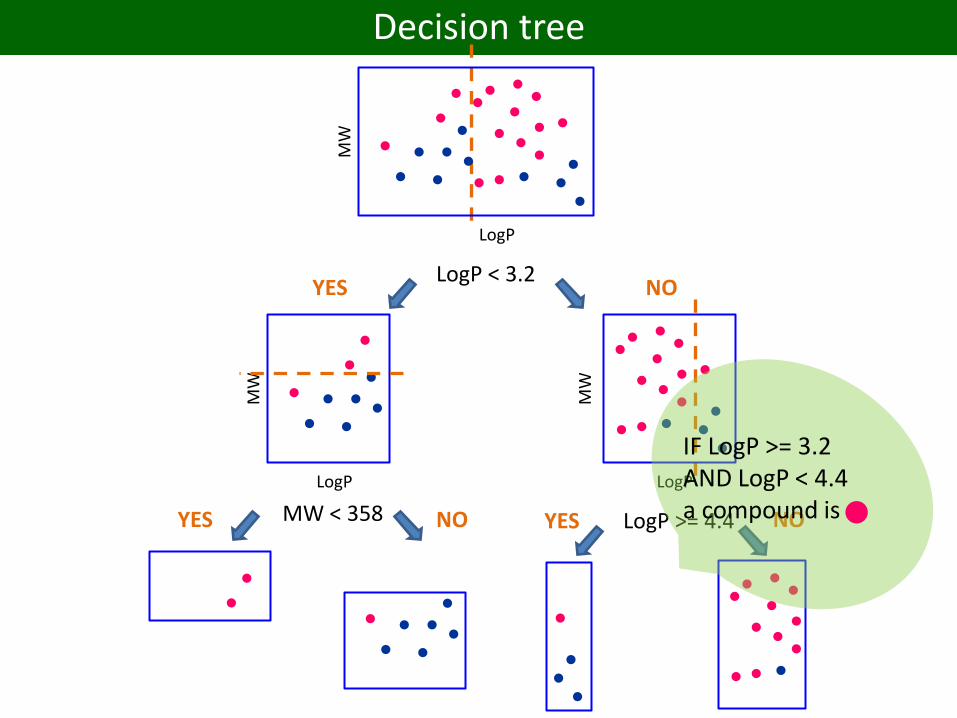
QSAR model building
18
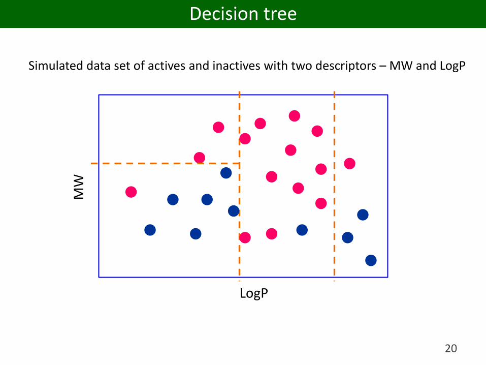
Simulated data set of actives and inactives with two descriptors – MW and LogP
LogP
MW
Decision tree
Decision tree
LogP
MW
LogP < 3.2YES NO
LogP
MW
LogP
MW
MW < 358YES NO LogP >= 4.4YES NO
IF LogP >= 3.2 AND LogP < 4.4 a compound is
20
Simulated data set of actives and inactives with two descriptors – MW and LogP
LogP
MW
Decision tree
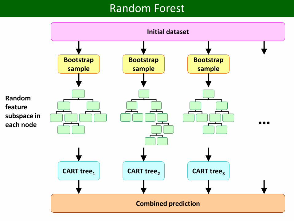
Initial dataset
Bootstrapsample
Bootstrapsample
Bootstrapsample
CART tree1 CART tree2 CART tree3
Combined prediction
…
Random feature subspace in each node
Random Forest
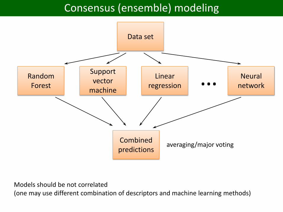
Consensus (ensemble) modeling
Data set
Random Forest
Support vector
machine
Linear regression
Neural network…
Combined predictions
Models should be not correlated(one may use different combination of descriptors and machine learning methods)
averaging/major voting

Consensus (ensemble) modeling
Data set
Random Forest
Support vector
machine
Linear regression
Neural network…
Metamodel(linear regression)
stacking
Prediction
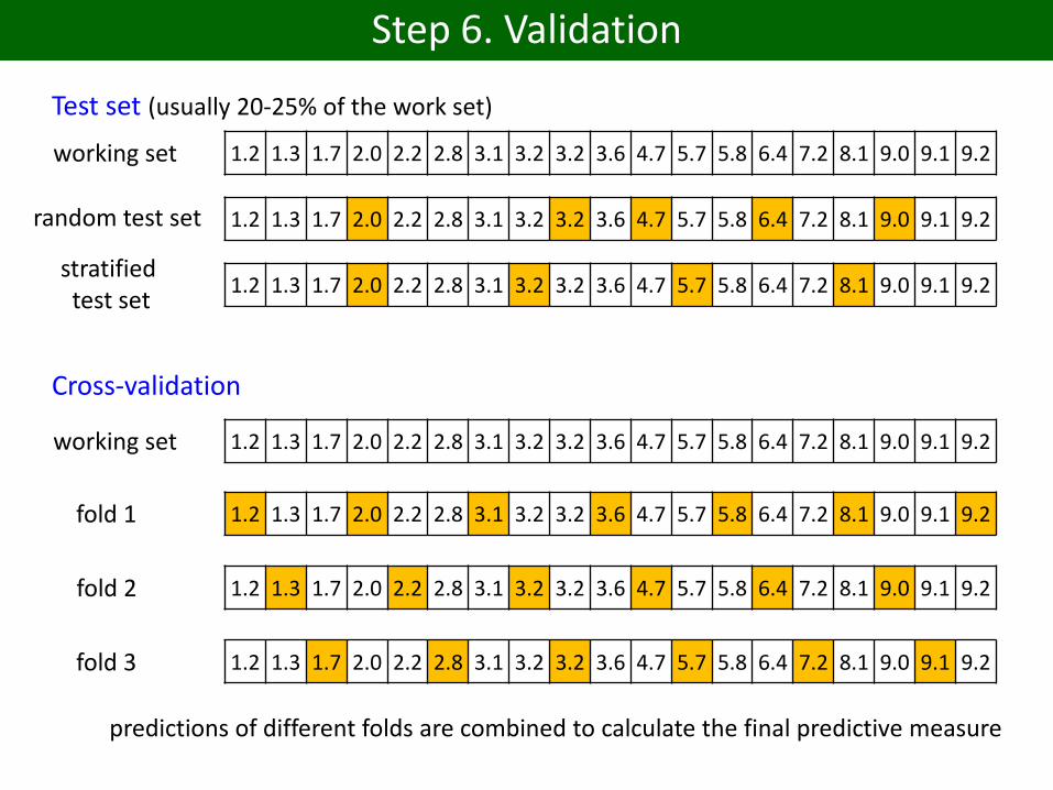
Step 6. Validation
Test set (usually 20-25% of the work set)
1.2 1.3 1.7 2.0 2.2 2.8 3.1 3.2 3.2 3.6 4.7 5.7 5.8 6.4 7.2 8.1 9.0 9.1 9.2working set
random test set 1.2 1.3 1.7 2.0 2.2 2.8 3.1 3.2 3.2 3.6 4.7 5.7 5.8 6.4 7.2 8.1 9.0 9.1 9.2
stratified test set
1.2 1.3 1.7 2.0 2.2 2.8 3.1 3.2 3.2 3.6 4.7 5.7 5.8 6.4 7.2 8.1 9.0 9.1 9.2
Cross-validation
1.2 1.3 1.7 2.0 2.2 2.8 3.1 3.2 3.2 3.6 4.7 5.7 5.8 6.4 7.2 8.1 9.0 9.1 9.2working set
1.2 1.3 1.7 2.0 2.2 2.8 3.1 3.2 3.2 3.6 4.7 5.7 5.8 6.4 7.2 8.1 9.0 9.1 9.2
1.2 1.3 1.7 2.0 2.2 2.8 3.1 3.2 3.2 3.6 4.7 5.7 5.8 6.4 7.2 8.1 9.0 9.1 9.2
1.2 1.3 1.7 2.0 2.2 2.8 3.1 3.2 3.2 3.6 4.7 5.7 5.8 6.4 7.2 8.1 9.0 9.1 9.2
fold 1
fold 2
fold 3
predictions of different folds are combined to calculate the final predictive measure
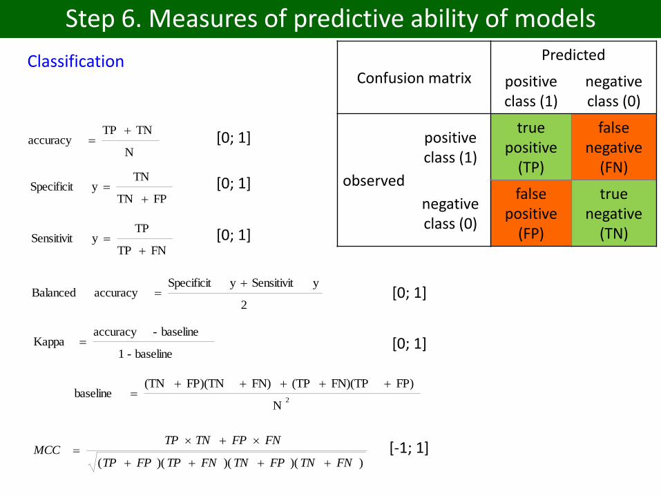
Step 6. Measures of predictive ability of models
Classification
FPTN
TNySpecificit
FNTP
TPySensitivit
2
ySensitivitySpecificitaccuracy Balanced
baseline-1
baseline -accuracy Kappa
N
TNTPaccuracy
2N
FP)FN)(TP(TPFN)FP)(TN(TNbaseline
Confusion matrix
Predicted
positive class (1)
negative class (0)
observed
positive class (1)
truepositive
(TP)
false negative
(FN)
negative class (0)
false positive
(FP)
true negative
(TN)
))()()(( FNTNFPTNFNTPFPTP
FNFPTNTPMCC
[-1; 1]
[0; 1]
[0; 1]
[0; 1]
[0; 1]
[0; 1]
Step 6. Measures of predictive ability of models
Regression
i
2
obspredi,
i
2
obsi,predi,
2
)y(y
)y(y
1Q
1N
)y(y
RMSEi
2
obsi,predi,
N
1i
obsi,predi,yy
N
1MAE
Determination coefficient
Root mean squared error
Mean absolute error

Step 7. Applicability domain (AD)Extrapolation to very distant objects is dangerous
There is a need to define the domain where our model is reliable (models are not universal!)
Only compounds which are similar to the training set compounds should be included in applicability domain of the model. One should estimate similarity of new compounds (test set, etc) to the training set compounds.
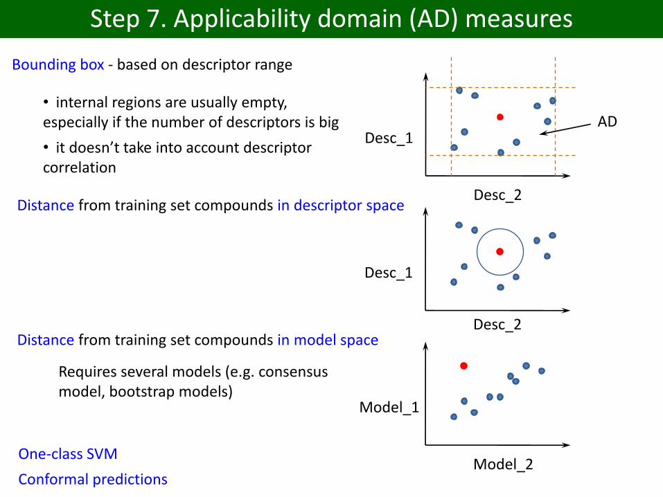
Step 7. Applicability domain (AD) measures
Bounding box - based on descriptor range
Desc_1
Desc_2
AD• internal regions are usually empty, especially if the number of descriptors is big
• it doesn’t take into account descriptor correlation
Distance from training set compounds in descriptor space
Desc_1
Desc_2Distance from training set compounds in model space
Model_1
Model_2
Requires several models (e.g. consensus model, bootstrap models)
One-class SVM
Conformal predictions

Step 7. Applicability domain (AD) example
J. Chem. Inf. Model., Vol. 50, No. 12, 2010
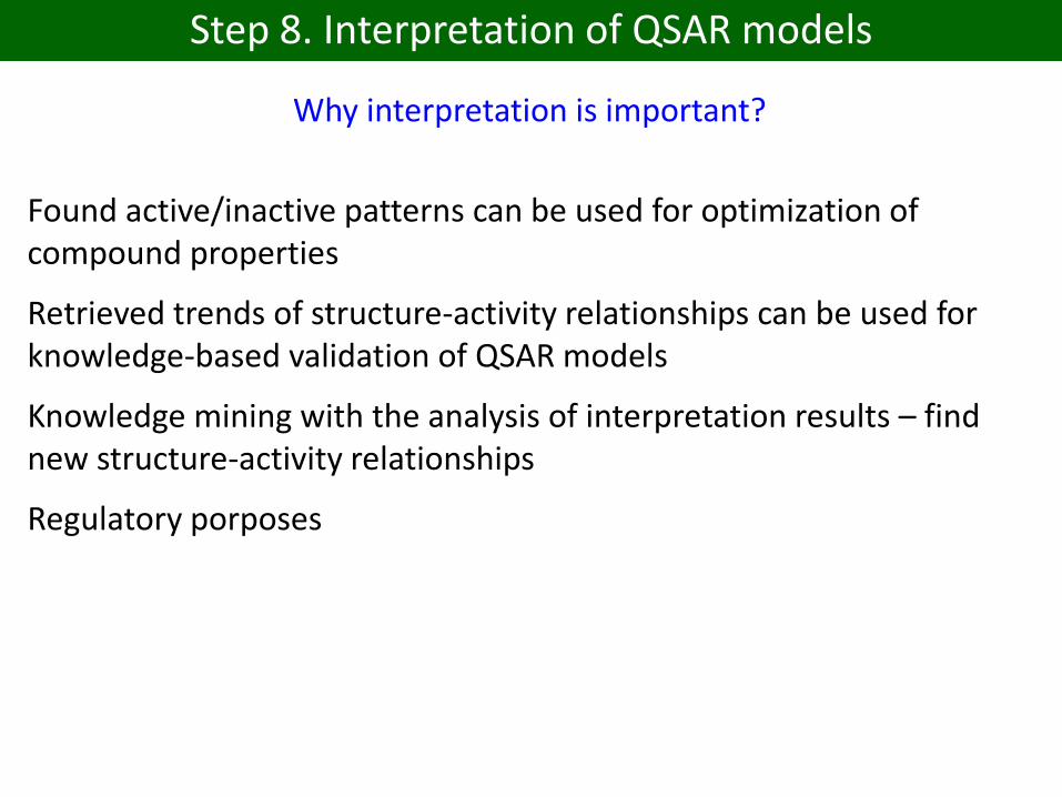
Step 8. Interpretation of QSAR models
Found active/inactive patterns can be used for optimization of compound properties
Retrieved trends of structure-activity relationships can be used for knowledge-based validation of QSAR models
Knowledge mining with the analysis of interpretation results – find new structure-activity relationships
Regulatory porposes
Why interpretation is important?
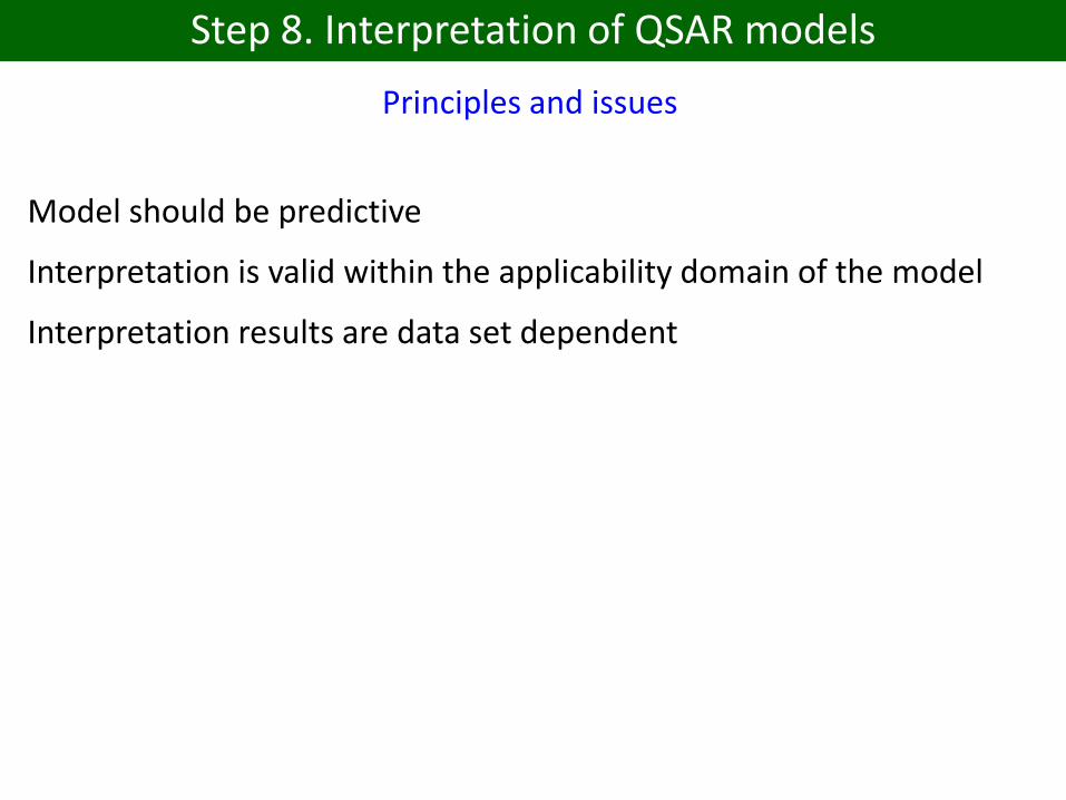
Step 8. Interpretation of QSAR models
Principles and issues
Model should be predictive
Interpretation is valid within the applicability domain of the model
Interpretation results are data set dependent
Step 8. Interpretation of QSAR models
1/C = 4.08π – 2.14π2 + 2.78σ + 3.38
π = logPX – logPH
σ - Hammet constant
plant growth inhibition activity of phenoxyacetic acids
electronic factorsrate of penetration of membranes in the plant cell
Hansch equation
R is H or CH3;
X is Br, Cl, NO2 and
Y is NO2, NH2, NHC(=O)CH3
Inhibition activity of compounds against Staphylococcus aureus
Act = 75RH – 112RCH3 + 84XCl – 16XBr – 26XNO2 + 123YNH2 + 18YNHC(=O)CH3 – 218YNO2
Free-Wilson models

-2
-2
-1
0
2
4
4
1
Step 8. Interpretation of QSAR models
2 δ
δ)f(xδ)f(xC
f(x)δ)f(xC
δ)f(xf(x)C
forward difference
backward difference
central difference
Partial derivatives is used to calculate contributions of single features.It is applicable to any model built on meaningful (interpretable) descriptors.May be calculated analytically or numerically.
Estimated contributions of separate substructural features can be mapped back on the structure to reveal contribution of fragments.
C-C-N -3
C-C-O +6
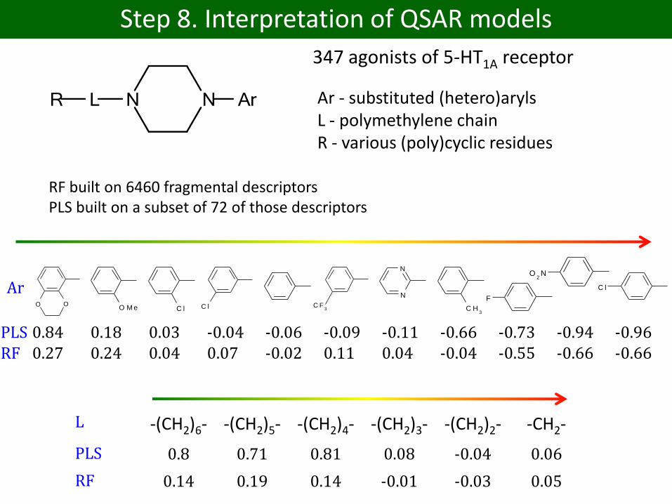
Step 8. Interpretation of QSAR models
347 agonists of 5-HT1A receptor
Ar - substituted (hetero)arylsL - polymethylene chainR - various (poly)cyclic residues
O OO M e C l C l C F
3
N
N
C H3
F
O2N
C l
PLS 0.84 0.18 0.03 -0.04 -0.06 -0.09 -0.11 -0.66 -0.73 -0.94 -0.96RF 0.27 0.24 0.04 0.07 -0.02 0.11 0.04 -0.04 -0.55 -0.66 -0.66
Ar
L -(CH2)6- -(CH2)5- -(CH2)4- -(CH2)3- -(CH2)2- -CH2-
PLS 0.8 0.71 0.81 0.08 -0.04 0.06
RF 0.14 0.19 0.14 -0.01 -0.03 0.05
RF built on 6460 fragmental descriptorsPLS built on a subset of 72 of those descriptors
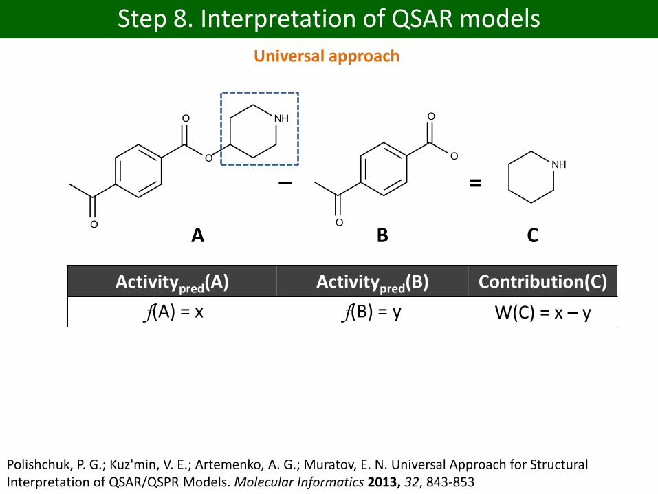
Step 8. Interpretation of QSAR models
=–
A B C
Activitypred(A) Activitypred(B) Contribution(C)
f(A) = x f(B) = y W(C) = x – y
Polishchuk, P. G.; Kuz'min, V. E.; Artemenko, A. G.; Muratov, E. N. Universal Approach for Structural Interpretation of QSAR/QSPR Models. Molecular Informatics 2013, 32, 843-853
Universal approach
Step 8. Interpretation of QSAR models
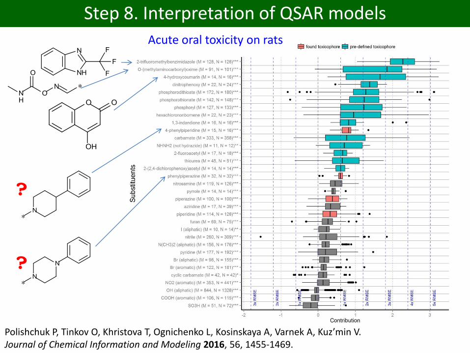
Polishchuk P, Tinkov O, Khristova T, Ognichenko L, Kosinskaya A, Varnek A, Kuz’min V. Journal of Chemical Information and Modeling 2016, 56, 1455-1469.
Acute oral toxicity on rats
?
?
Step 8. Interpretation of QSAR models
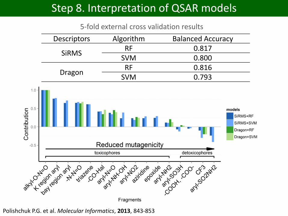
Descriptors Algorithm Balanced Accuracy
SiRMSRF 0.817
SVM 0.800
DragonRF 0.816
SVM 0.793
5-fold external cross validation results
Polishchuk P.G. et al. Molecular Informatics, 2013, 843-853
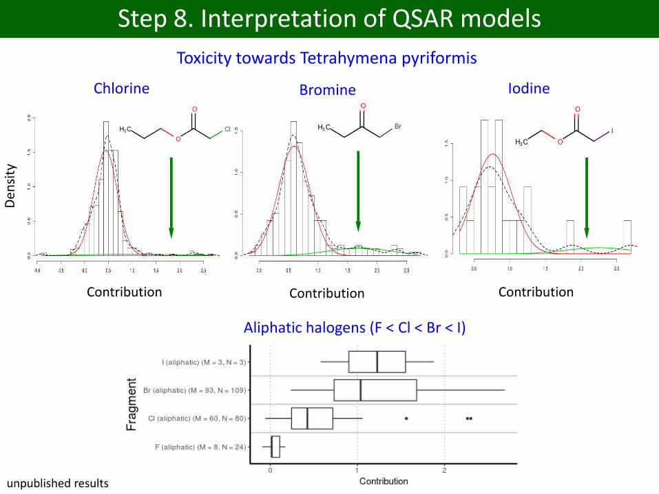
Chlorine Bromine Iodine
Den
sity
ContributionContributionContribution
Aliphatic halogens (F < Cl < Br < I)
unpublished results
Step 8. Interpretation of QSAR models
Toxicity towards Tetrahymena pyriformis
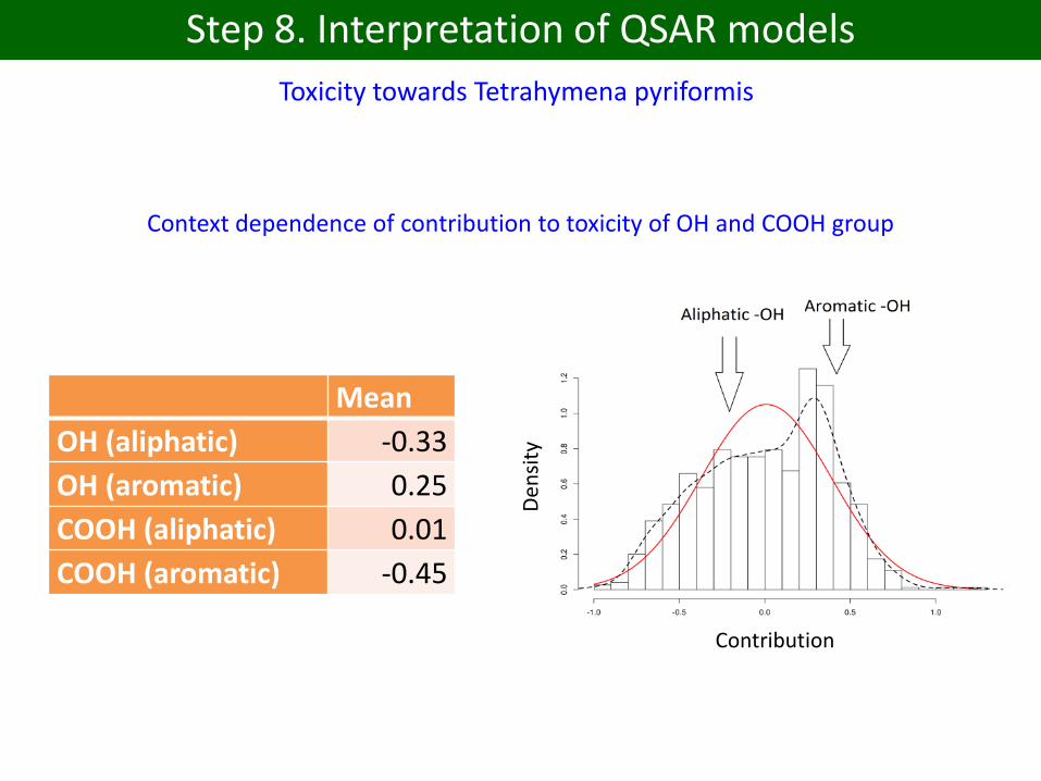
Step 8. Interpretation of QSAR models
Mean
OH (aliphatic) -0.33
OH (aromatic) 0.25
COOH (aliphatic) 0.01
COOH (aromatic) -0.45
Contribution
Den
sity
Context dependence of contribution to toxicity of OH and COOH group
Toxicity towards Tetrahymena pyriformis

Case
number
Do specific interactions of a ligand
with its target exist or important?
Is an orientation of
a ligand relatively
its target known?
Fragments selection
and grouping
1
NO
(e.g. passive diffusion through mem-
branes, solubility, lipophilicity, etc)
not relevant
can be done by the
researcher based on his
own knowledge
2
YES
(ligand-receptor interactions,
host-guest complexes, etc)
YES
consider fragments’
positions relatively to
the target and observed
or predicted
interactions
3 NO
MMP can be applied,
silently assumed that all
compounds have the
same interaction mode
Step 8. Interpretation of QSAR models
Step 8. Interpretation of QSAR models: conclusions
Interpretation results of a good predictive model should converge independent of:
interpretation approachdescriptorsmachine learning method
All models are interpretable but not all end-points
Overall QSAR workflow
Input data
Bioassays
Databases
PreprocessingFeature
engineeringModel
learningModel
validation
Classification
Regression
Clustering
Cross-validation
Bootstrap
Test set
Applicability Domain
Feature selection
Feature combination
Data normalization
Feature extraction
Interpretation
j
j
i
i
z
xxx
'
Pharmacophore modeling
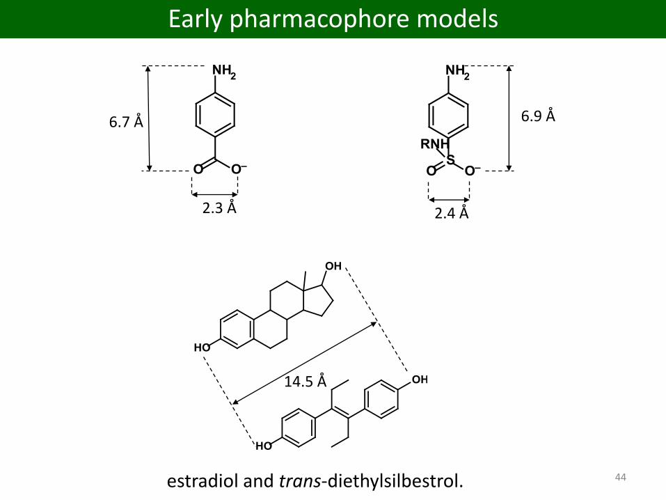
2.4 Å
estradiol and trans-diethylsilbestrol.
14.5 Å
2.3 Å
6.7 Å 6.9 Å
44
Early pharmacophore models
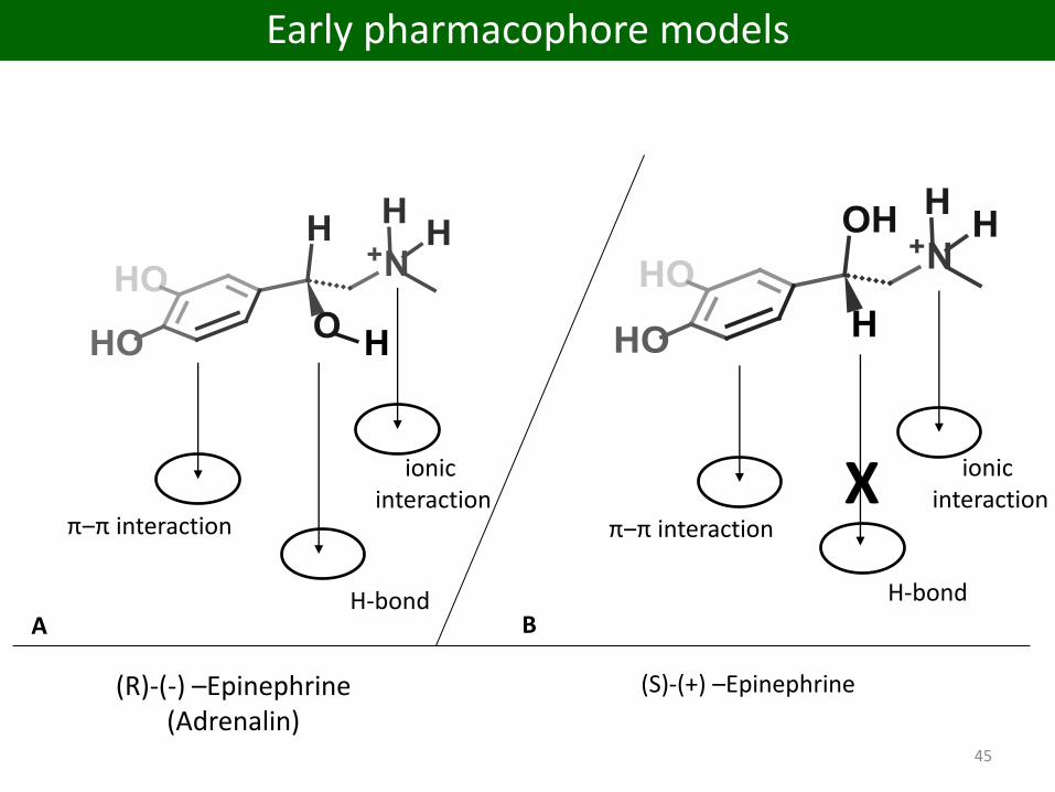
ionic interaction
H-bond
π‒π interaction
ionic interaction
H-bond
π‒π interaction
X
A B
45
(R)-(-) –Epinephrine(Adrenalin)
(S)-(+) –Epinephrine
Early pharmacophore models
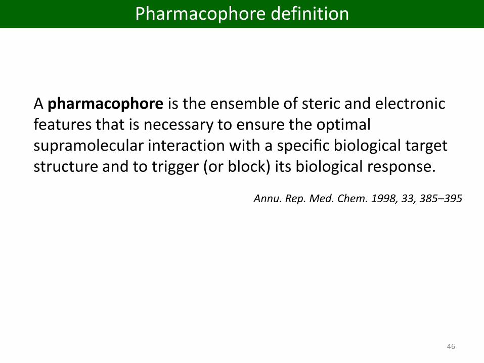
A pharmacophore is the ensemble of steric and electronic features that is necessary to ensure the optimal supramolecular interaction with a specific biological target structure and to trigger (or block) its biological response.
Annu. Rep. Med. Chem. 1998, 33, 385–395
46
Pharmacophore definition
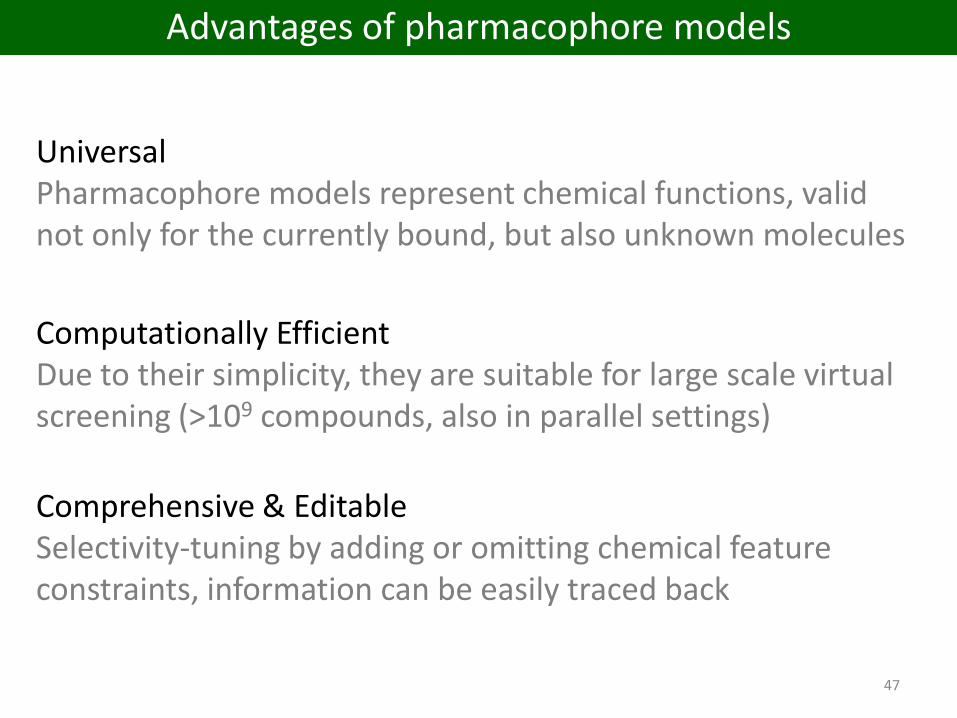
UniversalPharmacophore models represent chemical functions, valid not only for the currently bound, but also unknown molecules
Computationally EfficientDue to their simplicity, they are suitable for large scale virtual screening (>109 compounds, also in parallel settings)
Comprehensive & EditableSelectivity-tuning by adding or omitting chemical feature constraints, information can be easily traced back
47
Advantages of pharmacophore models
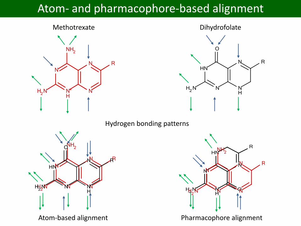
Atom- and pharmacophore-based alignment
Methotrexate Dihydrofolate
Hydrogen bonding patterns
Atom-based alignment Pharmacophore alignment
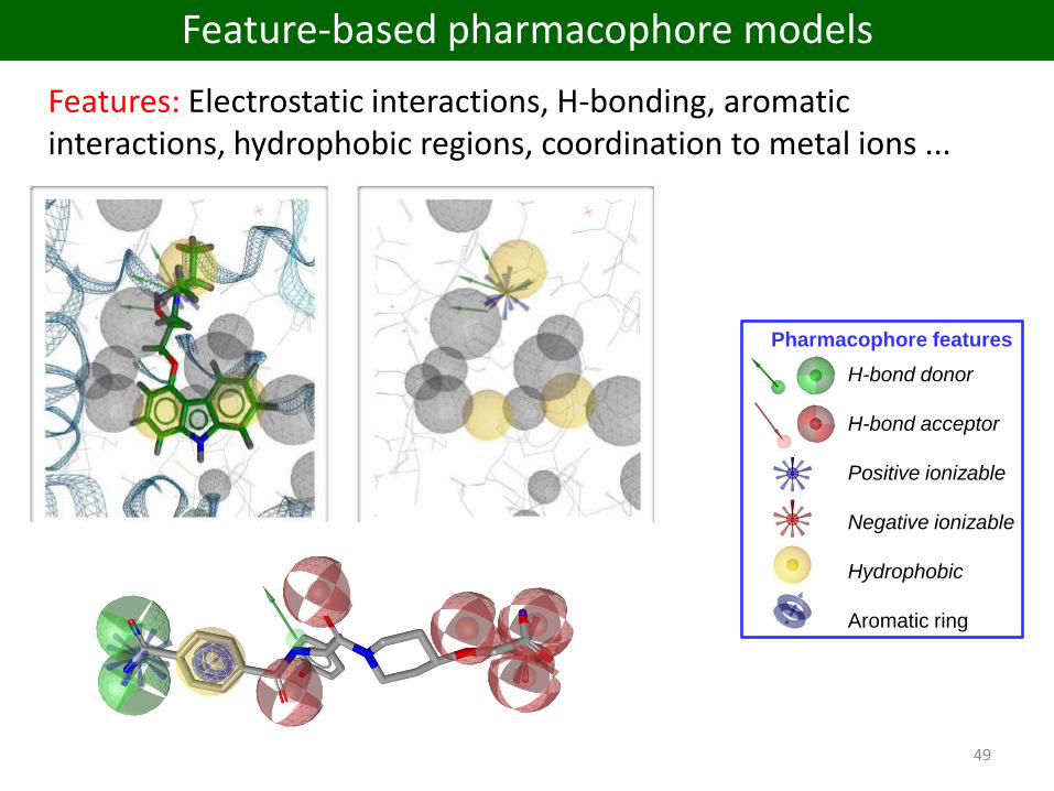
Features: Electrostatic interactions, H-bonding, aromatic interactions, hydrophobic regions, coordination to metal ions ...
49
Feature-based pharmacophore models
H-bond donor
H-bond acceptor
Positive ionizable
Negative ionizable
Hydrophobic
Aromatic ring
Pharmacophore features
Ligand-based pharmacophore
Exploration of conformational space
Multiple superpositioning experiments
DISCO, Catalyst, Phase, MOE, Galahad, LigandScout ...
Structure-based pharmacophore
GRID interaction fields: Convert regions of high interaction energy into pharmacophore point locations & constraints[S. Alcaro et al., Bioinformatics 22, 1456-1463, 2006]
Start from target-ligand complex: Convert interaction pattern into pharmacophore point locations & constraints[G. Wolber et al., J. Chem. Inf. Model. 45, 160-169, 2005]
50
Ligand- and structure-based pharmacophores
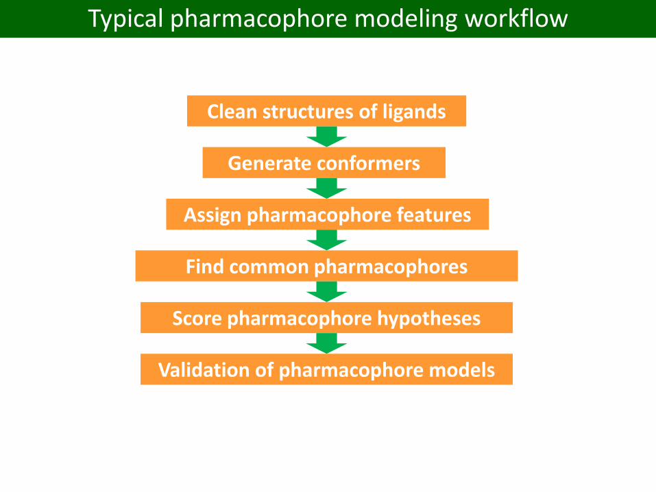
Typical pharmacophore modeling workflow
Clean structures of ligands
Generate conformers
Assign pharmacophore features
Find common pharmacophores
Score pharmacophore hypotheses
Validation of pharmacophore models
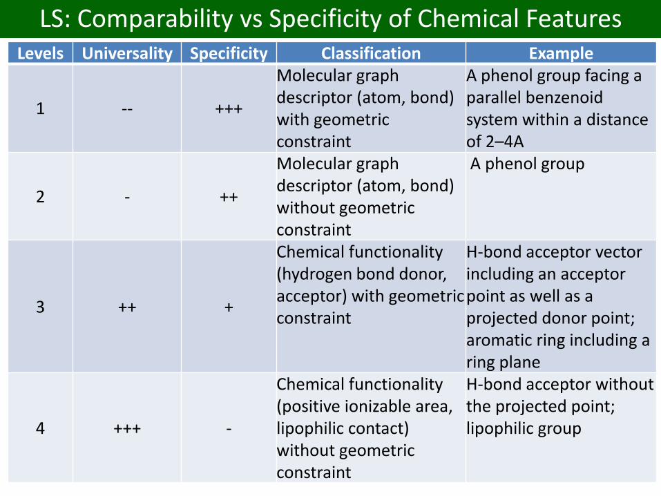
LS: Comparability vs Specificity of Chemical FeaturesLevels Universality Specificity Classification Example
1 -- +++
Molecular graph descriptor (atom, bond) with geometric constraint
A phenol group facing a parallel benzenoidsystem within a distanceof 2–4A
2 - ++
Molecular graph descriptor (atom, bond) without geometric constraint
A phenol group
3 ++ +
Chemical functionality (hydrogen bond donor,acceptor) with geometric constraint
H-bond acceptor vector including an acceptor point as well as a projected donor point; aromatic ring including a ring plane
4 +++ -
Chemical functionality (positive ionizable area, lipophilic contact) without geometric constraint
H-bond acceptor without the projected point; lipophilic group
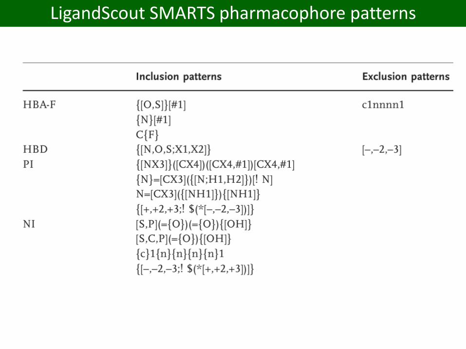
LigandScout SMARTS pharmacophore patterns
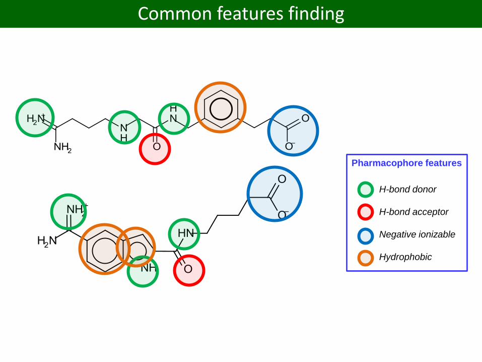
Common features finding
H-bond donor
H-bond acceptor
Negative ionizable
Hydrophobic
Pharmacophore features
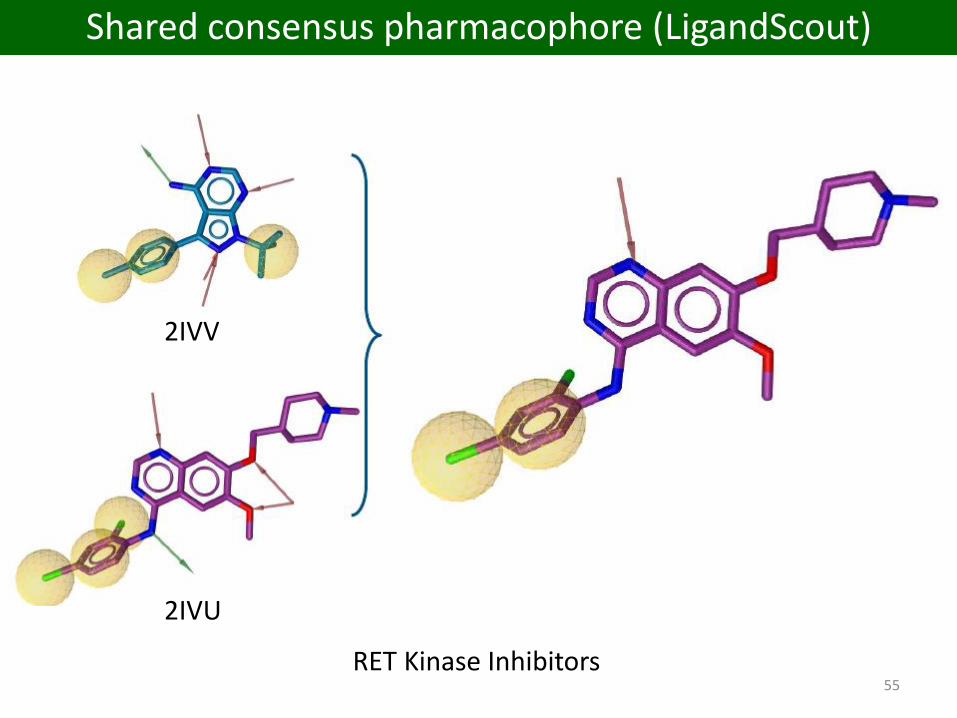
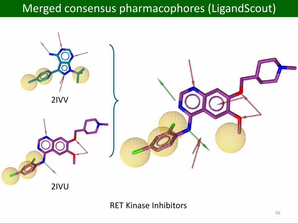
55RET Kinase Inhibitors
2IVU
2IVV
Shared consensus pharmacophore (LigandScout)
56RET Kinase Inhibitors
2IVU
2IVV
Merged consensus pharmacophores (LigandScout)
Validation with external test set
57
Observed
0 1
Pre
dic
ted 0 TN FN
1 FP TP
Pharmacophore validation
Negatives Positives
1
InactivesActives
Nu
mb
er o
f co
mp
ou
nd
s
Threshold Si Fit score 0 11-Sp
Se
AUC = 0-1
InactivesActives
Nu
mb
er o
f co
mp
ou
nd
s
Threshold Si Fit score 0 11-Sp
Se
AUC = 1
Inactives
Actives
Nu
mb
er o
f co
mp
ou
nd
s
Threshold Si Fit score 0 11-Sp
Se
1
AUC =0.5
58
1
Pharmacophore validation: ROC
Decision making from ROC curves
1
0 11-Sp
Se
InactivesActives
Break-even strategyOptimize both Se and Sp
S2
Inactives
Actives
Conservative strategyIncrease the hit rate
Faster, cheaper, motivating
S3
InactivesActives
Liberal strategyIncrease chemical diversity
Innovative
S1
59
Pharmacophore validation: ROC

60
Liga
nd
s
Pharmacophore models
Pharmacophore: ligand profiling
T. Steindl et al., J. Chem. Inf. Model., 46, 2146-2157 (2006)
61
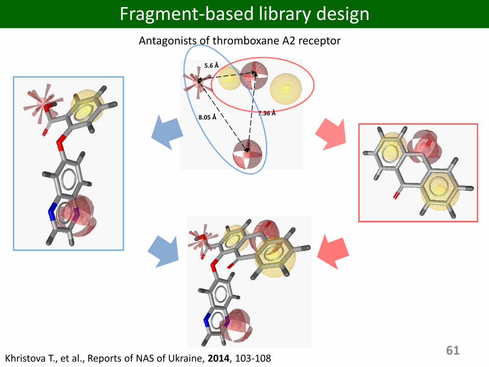
8.05 Å7.36 Å
5.6 Å
Fragment-based library designAntagonists of thromboxane A2 receptor
Khristova T., et al., Reports of NAS of Ukraine, 2014, 103-108
62
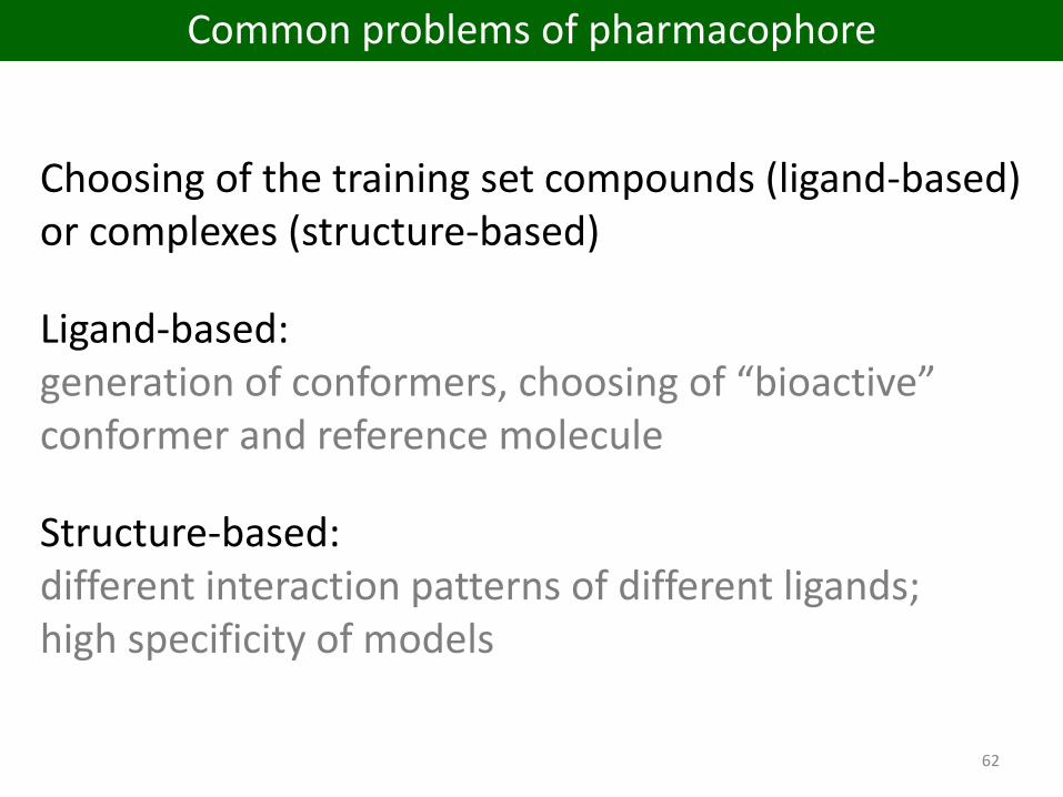
Choosing of the training set compounds (ligand-based) or complexes (structure-based)
Ligand-based:generation of conformers, choosing of “bioactive” conformer and reference molecule
Structure-based:different interaction patterns of different ligands;high specificity of models
Common problems of pharmacophore
63
Pharmacophores and Pharmacophore SearchesEds.: Thierry Langer, Rémy D. Hoffmann2006
Recommended literature
64
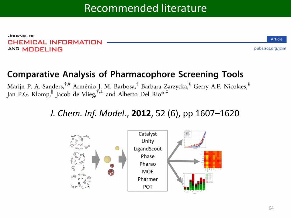
J. Chem. Inf. Model., 2012, 52 (6), pp 1607–1620
Recommended literature