ApPENDIX F

Q, erf & erfc Functions

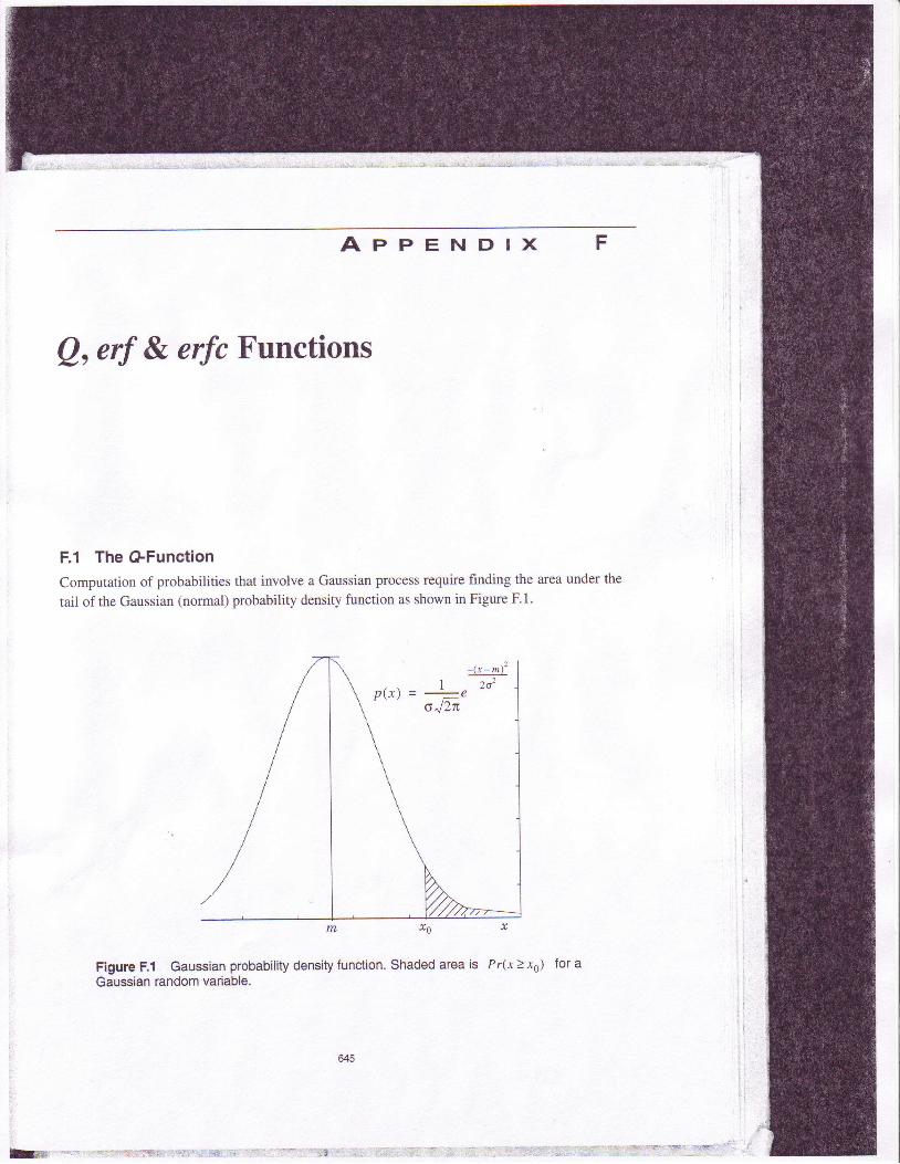
F.l The GFunctionComputation of probabilities that involve a Gaussian process require finding the area under the

tail of the Gaussian (normal) probability density function as shown in Figure F.l.

trL J$ x

Figure F.l Gaussian probability density function. Shaded area is Pr(x> xs)Gaussian random variable.

for a

Appendix F . Q, ert & erfc Functions

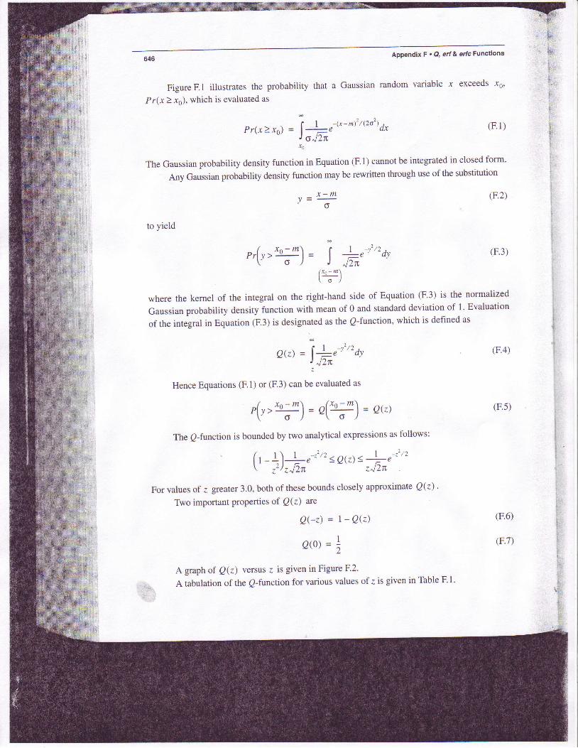
Figure F.l illustrates the probability that a Gaussian random variable .r exceeds x0,

Pr(x>.rs), which is evaluated as

' | 1 - r x - m t : / \ 2 o 2 t *P r \ x 2 x o ) = l - et 6 "J /.TE

(F.1)

(F.2)

(F.3)

(F.4)

(F.5)

(F.6)

(F.7)

r0

The Gaussian probability density function in Equation (F.1) cannot be integrated in closed form'

Any Gaussian probability density function may be rewritten through use of the substitution

to yield

x - my = -- o

r,(r> ry)= j f-^'-r"o'( x o - m \

\ o l

where the kernel of the integral on the right-hand side of Equation (F.3) is the normalized

Gaussian probability density function with mean of 0 and standard deviation of 1. Evaluation

of the integral in Equation (F.3) is designated as the Q-function, which is defined as

o(:) = 11,'"'a,J rJ2n

Hence Equations (F.1) or (F.3) can be evaluated as

/ x^-m\ ( ro- . ! \ = o(z \. l r t -J =g( . -o ) -

The o-function is bounded by two analytical expressions as follows:

/ r \ | - l t 1 - . 2 , )

I r _1 l * " - " ' <QQ)3 - i - e ' -

\ , 'z)7J2n zJTn

For values of z greater 3.0, both of these bounds closely approximate Q(z) .

Two important properties of Qk) are

Qer) = r -QQ)

O0 =,

A graph of Qk) versus { is given in Figure F 2'

A tabulation of the Q-function for various values of z is given in Table F.l.

t-,

il :*.i :::{ :

t;i,:t

The O+unction

Table F.1 Tabulation of the Gfunction

aQl aQ)

0.50000 2.0 0.02275

0.1 0.46017 2 .1 0.01786

0.42074 2.2 0.0r390

0.38209 2.3 0.01072

0.4 0.34458 0.00820

0.30854 2.5 0.00621

0.27425 2.6 0.00466

0.24t96 2.7 0.00347

0.21 I 86 2.8 0.00256

0.1 8406 2.9 0.00187

0.1 5866 3.0 0.00135

0.13567 J . l 0.00097

0.1 1507 0.00069

l . J 0.09680 J . J 0.00048

0.08076 3 . +

0.06681 3.5 0.00023

0.05480 3.6 0.00016

0.04457 3.7

0.03593 3.8

0.02872 3.9

0.0

0.2

0.3

0.5

0.6

0.7

0.8

0.9

1 .0

l . l

) . 2r.2

0.000341.4

1 .5

t . o

t t 0.00011

1 , 8 0.00007

1 .9

i :i

f'v .FL

* t -ta*,*.- . .

'0.00005

0 0.5 1.0 1.5 2.0 2.5

Figure F.2 Plot of the Glunction.

erfc(z) = t-erf(z)

F.2 The erf and ertc FunctionsThe enor function (erf; is defined as

n 'er.f(a) = 4lr-" a,

J"t,

and the complementary error function (erfc) is defined as

" i - 2

er fc \z) = ! - le-^ drJnr,

The erfc function is related to the et'function by

Appendix F . Q, ert & ertc Functions

(F.10)

f

, . 'Lf.t 't

-lt 0

10-'

(F.8)

(F.9)

The erfand elc Function

The Q-function is related to the erf and erfc functions by

l T / z \ ) I / - \

Qc) = ; l t -er \ ; , l l = ; , ,J , l i ). 4 2 . , - . 4 2 ,

erfc(z) = 2Q(J1z)

er f (z) = 1-2Q0J2z)

The relationships in Equations (F.1 1)-(F.13) are widely used in eror probability computa-

tions. Table F.2 displays values for the e f function.

Table F.2 Tabulation of the Error Function erf(z)

z ertQl z ertQl

0.1 0.1t246 1.6 0.97635

0.2 0.22270 l ' 1 0.98379

0.32863 1 . 8 0.98909

0.4 0.42839 1 . 9 0.992'79

0.-5 0.52049 2.0 0.99532

0.6 0.60385 2 . 1 0.99702

0.67780 2.2 0.99814

0.8 0.74210 L . 3 0.99885

0.79691 . A 0.99931

0.842'70 2.5 0.99959

1 . 1 0.88021 2.6 0.99976

0.91031 2.1 0.99987

l . J 0.93401 2.8 0.99993

1 . 4 0.95228 2.9 0.99996

(F .11)

(F.12)

/ E I ? . \

0.7

0.9

i . 0

t .2

, .:.,

t

Tl :a.

I?,1:.:i :-r+:it.w

1 . 5 0.9661r 3.0 0.99998