Python Tutorial DocumentationRelease 1

Jinbo Wang

March 11, 2013

CONTENTS

1 Introduction 31.1 What do we need . . . . . . . . . . . . . . . . . . . . . . . . . . . . . . . . . . . . . . . . . . . . . 31.2 Python language . . . . . . . . . . . . . . . . . . . . . . . . . . . . . . . . . . . . . . . . . . . . . 31.3 Software packages . . . . . . . . . . . . . . . . . . . . . . . . . . . . . . . . . . . . . . . . . . . . 41.4 Demo . . . . . . . . . . . . . . . . . . . . . . . . . . . . . . . . . . . . . . . . . . . . . . . . . . . 5

2 popy - The Python package for Physical oceanographer 9

i

ii

Python Tutorial Documentation, Release 1

Table of Contents

CONTENTS 1

Python Tutorial Documentation, Release 1

2 CONTENTS

CHAPTER

ONE

INTRODUCTION

Table of Contents

• Introduction– What do we need– Python language– Software packages– Demo

* Work with netcdf files and Basemap* Work with matlab files and mayavi2* Animate your data in 3D in realtime

Note: Prepared by Jinbo Wang for the vis-club at Scripps Institution of Oceanography (03/11/2013)

1.1 What do we need

• load/generate data

• manipulate and process data

• visualize results

1.2 Python language

• interpreted language, no compilation

• modulized, shorter scripts

• multiplatform, (Windows, Linux, MacOs X)

• easy interface with other language, such as C and fortran

• open-source

• large variety of packages for various applications

3

Python Tutorial Documentation, Release 1

1.3 Software packages

What I freqently used:

• numpy, for numerical calculation http://www.numpy.org/

• a powerful N-dimensional array manipulation

• sophisticated (broadcasting) functions

• tools for integrating C/C++ and Fortran code

• useful linear algebra, Fourier transform, and random number capabilities

• SciPy scientific tools for Python. http://www/scipy.org

• depends on numpy

• large collection of science and engineering modules

• Special functions (scipy.special)

• Integration (scipy.integrate)

• Optimization (scipy.optimize)

• Interpolation (scipy.interpolate)

• Fourier Transforms (scipy.fftpack)

• Signal Processing (scipy.signal)

• Linear Algebra (scipy.linalg)

• Sparse Eigenvalue Problems (scipy.sparse)

• Statistics (scipy.stats)

• Multi-dimensional image processing (scipy.ndimage)

• File IO (scipy.io)

• easy netcdf and matlab interface:

• scipy.io.netcdf scipy.io.loadmat scipy.savemat

• Ipython interactive computing, gives Matlab-like environment and more http://ipython.org

• matplotlib 2D plotting library, http://matplotlib.org

• easy to use but highly configurable

• hugh collection of examples http://matplotlib.org/gallery.html

• produces publication quality figures in a variety of hardcopy formats (png, jpeg, ps, eps, svg, pdfetc.)

• Basemap similar to matlab mapping toolbox. examples

• mayavi2 3D plotting http://docs.enthought.com/mayavi/mayavi/

• based on VTK

• simple and clean interface

• natural extention of matplotlib

• many examples

• seawater identical to matlab seawater toolbox

4 Chapter 1. Introduction

Python Tutorial Documentation, Release 1

• sphinx for documentation

• use reStructuredText (rst)

• output html, Latex, Texinfo, manual page, plain text

• can link with python code, auto include matplotlib figures

• os: operating system interfaces

• sys: System-specific parameters and functions

Note: The Enthought Python Distribution (EPD) might the easiest solution for MacOs X and Windows users.

1.4 Demo

1.4.1 Work with netcdf files and Basemap

from scipy.io import netcdf_file as ncfn = "/Users/jbw/Project/Collection/OBS/WOA05/t0112an1.nc"

d = nc(fn,’r’) # return a handle to the nc fileprint d.variables # print variables in the nc filedef r(varname):

return d.variables[varname][:]

lon, lat, depth, time = r(’lon’),r(’lat’),r(’depth’),r(’time’)

from numpy import matemp = ma.masked_greater(r(’t0112an1’),1e4)

print temp.shape,lon.shape,lat.shape

from mpl_toolkits.basemap import Basemapimport numpy as np # from numpy import *import matplotlib.pyplot as plt# lon_0, lat_0 are the center point of the projection.# resolution = ’l’ means use low resolution coastlines.m = Basemap(projection=’ortho’,lon_0=-125,lat_0=-30,resolution=’l’)m.drawcoastlines()m.fillcontinents(color=’gray’,lake_color=’blue’)# draw parallels and meridians.m.drawparallels(np.arange(-90.,120.,30.))m.drawmeridians(np.arange(0.,420.,60.))m.drawmapboundary(fill_color=’white’)x,y = m(*np.meshgrid(lon,lat))m.contourf(x,y,temp[:,0,:,:].mean(axis=0),50,cmap=plt.cm.jet)cb=m.colorbar()cb.set_label(’Temperature $(^oC)$’)plt.title("Mean SST on Orthographic Projection")plt.show()

1.4. Demo 5

Python Tutorial Documentation, Release 1

Mean SST on Orthographic Projection

0

4

8

12

16

20

24

28

Tem

pera

ture

(oC

)

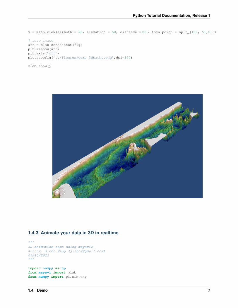
1.4.2 Work with matlab files and mayavi2

"""3D view of the bathymetry used in SOSEAuthor: Jinbo Wang <jinbow@gmail.com>"""from scipy.io import loadmatdatapath = ’/Users/jbw/Project/Workspace/Scripps/sose/data/GRID/grid.mat’

f = loadmat(datapath)print ’XC.shape = ’, f[’XC’].shape

data = f[’Depth’]*-1x,y = f[’XC’], f[’YC’]

# Plot ##################################################from mayavi import mlabimport matplotlib.pylab as pltimport numpy as np

warp_scale = 0.003fig = mlab.figure(size=(800, 600), bgcolor=(0.16, 0.28, 0.46))mlab.surf(x, y, data, colormap=’gist_earth’, warp_scale=warp_scale)#,vmin=-5700, vmax=5700)

6 Chapter 1. Introduction

Python Tutorial Documentation, Release 1

v = mlab.view(azimuth = 45, elevation = 50, distance =300, focalpoint = np.r_[180,-51,0] )

# save imagearr = mlab.screenshot(fig)plt.imshow(arr)plt.axis(’off’)plt.savefig(’../figures/demo_3dbathy.png’,dpi=150)

mlab.show()

1.4.3 Animate your data in 3D in realtime

"""3D animation demo using mayavi2Author: Jinbo Wang <jinbow@gmail.com>03/10/2023"""

import numpy as npfrom mayavi import mlabfrom numpy import pi,sin,exp

1.4. Demo 7

Python Tutorial Documentation, Release 1

import pylab as plt

def f(x,y,i):from scipy import specialreturn x*y*special.j1(i)

x, y = np.mgrid[-pi:pi:0.3,-pi:pi:0.3]s = mlab.surf(x, y, f(x,y,10),warp_scale="auto")mlab.savefig(’../figures/demo_3d_animation.png’)

for i in np.linspace(0,30*pi,300):s.mlab_source.scalars = np.asarray(f(x,y,i), ’d’)

8 Chapter 1. Introduction

CHAPTER

TWO

POPY - THE PYTHON PACKAGE FORPHYSICAL OCEANOGRAPHER

I am collecting/writing useful python modules, which will soon be published on github.com. Stay in tune.

9