Visualization in Python with matplotlib

Pete Alonzi

Research Data Services UVa Library

March 1, 2016

Check us outdata.library.virginia.edu

What we’re gonna do today

• 2-3:30

• Get everyone up and running with python

• python interfaces

• Loading matplotlib

• Plotting 101 (create and save)

• Histograms, scatter plots

• Cosmetics

• multiplots

Installation of Python

• Two Notes

– Language (python) vs language distribution (anaconda)

– Python 2 vs Python 3

• https://www.continuum.io/downloads

1. Scroll to your operating system

2. Click on the blue box under Python 2.7

3. Follow the instructions

Interfaces

• Command line interpreter (and ipython)

• Commandline script execution

• Ipython notebook / jupyter

• Spyder (generalize to ide)

Loading matplotlib

• It depends on your interface

A basic plot

• C: \Users \lpa2a>python• >>> import matplotlib.pyplot as plt

• >>> x=range(10)

• >>> plt.plot(x)

• >>> plt.show()

Why blue?

Why a line?

Why a line with slope of 1?

Why does it hang after show?

Saving a plot

• There are two ways to save the plot:

– Use the command line:

• >>> plt.savefig(‘test.pdf’)

• Must be done before the show command

– Use the gui:

• Click the save icon

• Type in the file name

• select the file type

Window control

• Notice when we use plt.show() we lose

control.

• To regain control we must close the plot

window.

• Now we’ll go through other ways of

interacting with matplotlib to avoid this

problem.

IPython + %pylab

• Instead of loading up python at the command line with python use ipython instead.

• Ipython has a special plotting mode which you load by issuing the command %pylab

• C:\Users\lpa2a>ipython• In [1]: %pylab• Now we can try our basic plot again.

– Don’t need to load matplotliab

– We don’t need to use the “plt.”– We don’t loose control when we plot

– Plot appears on plot command, no more show()

Command line scrip execution

• Let’s take a look at C:\Users\lpa2a\plot.py

Ipython Notebook

• Launch from start menu

• Click “New Notebook”

– In []: %pylab

– Or

– In []: %pylab inline

Spyder

• Runs the ipython interpreter

– Use %pylab or import

– Nb: cannot use “Run File” with %pylab

A quick note on appearance

• In the active plot window we observe a gray

border

• In the saved plot we observe a white border

Plot Generators

• There are a few functions in matplotlib that

will cause a plot to be generated.

• So far we have worked with plot(…) .

• Now we’ll look at a couple more

– hist(…)

– scatter(…)

Histograms

Histogram

• To plot a histogram we don’t use the function plot. We use the function hist– import numpy as np– import matplotlib.pyplot as plt– plt.hist(np.random.randn(1000))– plt.show()

• All of the tricks we just learned to manipulate the plot still work

• Here’s some examples for the binning– plt.hist(np.random.randn(1000),bins=25)– plt.hist(np.random.randn(1000),bins=[-

5,-4,-3,-2,-1,0,1,2,3,4,5])

17

Scatter Plot

• Use the function scatter()

– plt.scatter (np.random.randn (1000),np.random.randn (1000))

– If using pylab

– scatter( randn (1000), randn (1000 ))

18

plot(…)

• So far we have used a simple implementation of plot. Let’s look deeper.

• %pylab• plot(range(10)) #generates x values

• clf()• x=arange(0,2*pi,0.2)• plot(x,sin(x))

Multiplots

• To add multiple plots repeat the plot call

– %pylab

– x = arange(0,2*pi,0.2)

– plot1 = plot(x,sin(x))

– plot2 = plot(x,cos(x))

• Now to add a legend

– plot1 = plot(x,sin(x ),label=‘sin’)

– plot2 = plot(x,cos(x ),label=‘cos’)

– legend(loc=‘best’)

20

Subplots

• Multiple plots in the same figure

21

figure

Plot

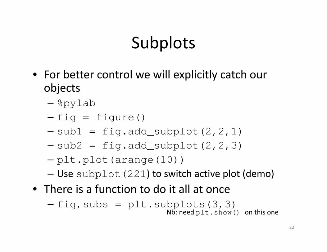
Subplots

• For better control we will explicitly catch our objects

– %pylab– fig = figure()– sub1 = fig.add_subplot(2,2,1)– sub2 = fig.add_subplot(2,2,3)– plt.plot(arange(10))

– Use subplot(221 ) to switch active plot (demo)

• There is a function to do it all at once

– fig,subs = plt.subplots(3,3)

22

Nb: need plt.show() on this one

Let’s make our plot presentable

• C:\users\lpa2a> ipython -- pylab

• In[1]: plot(cos(arange(0,2*pi,0.2 )))• Grey background

• Axis labels too small

• Plot touches axis

• Plot not centered on axis

• Horizontal axis values aren’t what we want

• No axis labels

• Line thickness

• Line style

23

Ranges and Values

• Set axis range

– axis([ -5,37, -1.5,1.5])

• Change horizontal axis values

– x=arange (0,2*pi,0.2)

– y=cos(x)

– plot( x,y )

24

Labels and LaTeX

• Set axis labels– xlabel(‘x’,fontsize=20)– ylabel(‘cos(x)’)– title(‘Cosine’)

• You can use LaTeX as well– title(r’$\cos(x)$’)

• http://matplotlib.org/users/pyplot_tutorial.html

25

Linestyles

• You have a lot of freedom in choosing a line

style.

• They can be expressed explicitly

– plot(x,linestyle=‘ -- ’)

• The same goes for line color

– plot(x,color=‘g’)

• But you can also use shorthand

– plot(x,’g -- ’)

26

Linestyles II

• matplotlib automatically interpolates between the points and puts in a line. To emphasize the points you can add markers.

– plot(range(10),’o’) # markers, no line

– plot(range(10),’o -’) # markers, line

– plot(range(10),marker=‘o’)

• Set line thickness

– pl = plot(arange(10))

– setp(pl,linewidth=5)

27

One Page to Rule them All

• http://matplotlib.org/api/pyplot_api.html

– Comprehensive

– Navigate with searching

– Eg: ctrl+f “.plot(“

Questions