Chapter 47 Animal Development. I. Fertilization A.Sea Urchins B.Mammals.
PURPLE SEA URCHINS (STRONGYLOCENTROTUS PURPURATUS) IN AND OUT
OF PITS: THE EFFECTS OF MICROHABITAT ON POPULATION STRUCTURE,
MORPHOLOGY, GROWTH, AND MORTALITY
by
BENJAMIN MICHAEL GRUPE
A THESIS
Presented to the Department of Biology
and the Graduate School of the University of Oregon
in partial fulfillment of the requirements
for the degree of
Master of Science
December 2006

ii
“Purple Sea Urchins (Strongylocentrotus purpuratus) in and out of Pits: the Effects of
Microhabitat on Population Structure, Morphology, Growth, and Mortality,” a thesis
prepared by Benjamin M. Grupe in partial fulfillment of the requirements for the Master
of Science degree in the Department of Biology. This thesis has been approved and
accepted by:
____________________________________________________________
Dr. Alan L. Shanks, Chair of the Examining Committee
________________________________________
Date
Committee in Charge: Dr. Alan L. Shanks, Chair
Dr. Thomas A. Ebert
Dr. Craig M. Young
Accepted by:
____________________________________________________________
Dean of the Graduate School
iii
An Abstract of the Thesis of
Benjamin Michael Grupe for the degree of Master of Science
in the Department of Biology to be taken December 2006
Title: PURPLE SEA URCHINS (STRONGYLOCENTROTUS PURPURATUS) IN AND
OUT OF PITS: THE EFFECTS OF MICROHABITAT ON POPULATION
STRUCTURE, MORPHOLOGY, GROWTH, AND MORTALITY
Approved: _______________________________________________
Dr. Alan L. Shanks
Purple sea urchins (Strongylocentrotus purpuratus) are common inhabitants of
wave-swept rocky shorelines on the Pacific Coast of North America. The effects of
microhabitat, inside and outside pits, were investigated in intertidal populations of S.
purpuratus. Nonpit urchins had significantly larger test diameters and spines, but pit
urchins had relatively larger test heights and jaw lengths, indicating possible food
limitation in pits. In a tetracycline-tagging study, nonpit urchins grew faster than pit
urchins. S. purpuratus in both microhabitats are long-lived and seldom moved, though age-
frequency distributions suggest that movement out of pits might occur between the ages of
five and ten. At South Cove, predation by oystercatchers, raccoons, and the sunflower sea
star Pycnopodia helianthoides was higher in nonpit microhabitats and is estimated to
account for most mortality of S. purpuratus. Mortality, growth, and morphology vary

iv
between microhabitats, which may have important consequences for populations of S.
purpuratus and other organisms.

v
CURRICULUM VITAE
NAME OF AUTHOR: Benjamin Michael Grupe
PLACE OF BIRTH: Cleveland, Ohio
DATE OF BIRTH: January 25, 1981
GRADUATE AND UNDERGRADUATE SCHOOLS ATTENDED:
University of Oregon, Oregon Institute of Marine Biology
Gettysburg College
DEGREES AWARDED:
Master of Science, 2006, University of Oregon
Bachelor of Arts, 2003, Gettysburg College
AREAS OF SPECIAL INTEREST:
Marine Community Ecology
Intertidal Ecology
PROFESSIONAL EXPERIENCE:
Teaching Assistant, Oregon Institute of Marine Biology, University of Oregon,
Charleston, 2006.
NSF GK-12 Graduate Teaching Fellow, Oregon Institute of Marine Biology,
University of Oregon, Charleston, 2004–2006.
Graduate Research Fellow, South Slough National Estuarine Research Reserve,
Charleston, Oregon, 2003–2004.
Laboratory assistant, Environmental Studies Department, Gettysburg College,
Gettysburg, Pennsylvania, 2002–2003.
vi
GRANTS, AWARDS AND HONORS:
Best Student Paper, Honorable Mention, Mia Tegner Ecology & Conservation
Award, Western Society of Naturalists Meetings, 2006.
Dr. Earl H. Myers and Ethel M. Myers Oceanographic and Marine Biology Trust,
The influence of microhabitat on the biology, morphology, and population
structure of the purple sea urchin Strongylocentrotus purpuratus, 2005.
National Science Foundation, GK-12 Graduate Teaching Fellowship, 2004–2006.
South Slough National Estuarine Research Reserve, Graduate Research
Fellowship, 2003–2004.
Phi Beta Kappa, Gettysburg College, 2003.
PUBLICATIONS:
Commito JA, Dow WE, Grupe BM (2006) Hierarchical spatial structure in soft-
bottom mussel beds. J Exp Mar Biol Ecol 330: 27-37

vii
ACKNOWLEDGMENTS
I wish to express my sincerest thanks to Alan Shanks, whose scientific prowess and
tutelage have dramatically improved my abilities as a scientist. An excellent advisor,
encourager, and mentor, Alan guided me through to the completion of a once-floundering
project, and for that I am grateful. This manuscript also benefited immensely from the
helpful comments I received from the other members of my graduate committee, Tom
Ebert and Craig Young. Their expertise in echinoids and hypothesis-driven science was
evident in their many suggestions and bits of advice that kept me on the right path.
I am thankful for the many hours of field work contributed by students and friends
of the Oregon Institute of Marine Biology, including Suzanna Stoike, Megan Copley,
Annie Pollard, Tracey Smart, Maya Wolf, Michelle Schuiteman, Shawn Arellano,
Stephanie Schroeder, Andy Bauer, Garrett Steinbroner, Tim Davidson, Kristin Parker, Jose
Marin Jarrin, and Kevin Anderson. Megan Copley deserves special mention for all her
assistance in the field and the lab, tolerance of bleach fumes, and especially for listening to
me blabber on about sea urchins for more hours than I can count. Encouraging
conversations with Jule Schultz, Jessica Miller, Jan Hodder, and Tim Davidson helped me
to define my research questions and advance my ideas. Dustin Marshall’s statistical
expertise was quite beneficial, and Barb Butler used her special librarian powers to
commandeer very useful aerial photos. I am forever indebted to Terrance Mann and
Archibald Graham for their wisdom, and even more so to my parents, family, and friends

viii
for their support. The late hours spent behind a microscope and writing would have been
much more tedious had it not been for Ryan Adams, Jeff Tweedy, Adam Duritz, Bruce
Springsteen, Ben Gibbard, and the 2006 World Champion St. Louis Cardinals. I thank all
of these people from the bottom of my heart.
Finally, I wish also to express gratitude towards my graduate funding sources: the
South Slough National Estuarine Research Reserve, the National Science Foundation, and
the Dr. Earl and Ethel Myers Oceanographic and Marine Biology Trust. Without their
assistance, we still would be unaware of the mysteries surrounding sea urchins and
microhabitat.

ix
To my parents, who first introduced me to the wonders of nature.
x
TABLE OF CONTENTS
Chapter Page
I. SEA URCHINS, HOLES IN THE ROCK, AND PUZZLES ......................................1
II. MICROHABITAT-BASED DIFFERENCES IN THE POPULATION
STRUCTURE AND MORPHOLOGY OF THE PURPLE SEA
URCHIN STRONGYLOCENTROTUS PURPURATUS ......................................4
Introduction ................................................................................................................4
Materials and Methods ..............................................................................................7
Study Sites and Sea Urchin Pits ..........................................................................7
Population Structure .............................................................................................9
Morphology .........................................................................................................10
Results .......................................................................................................................13
Population Structure ...........................................................................................13
Morphological Differences ................................................................................17
ANCOVA with Wet Mass as a Covariate .................................................17
ANCOVA with Test Diameter as a Covariate ..........................................24
Discussion ................................................................................................................28
Morphological Differences Indicate Microhabitat Fidelity ............................28
Nonpit Urchins Tend to Be Larger than Pit Urchins .......................................31
How Can the Differences in the Population Structure of
Strongylocentrotus purpuratus Between Microhabitats Be
Explained? ..............................................................................................34
Conclusion ...........................................................................................................39
Bridge to Chapter III ..........................................................................................40
III. DIFFERENTIAL GROWTH RATES OF STRONGYLOCENTROTUS
PURPURATUS INSIDE AND OUTSIDE PITS ................................................41
Introduction ..............................................................................................................41
Materials and Methods ............................................................................................44
Study Sites ...........................................................................................................44
Mark-Recapture Methods ..................................................................................46
Growth in Sites and Microhabitats ....................................................................49
Growth Model .....................................................................................................51
The Tanaka Growth Function ....................................................................51
Applying the Tanaka Function to the Growth Data .................................54

xi
Chapter Page
Age Estimation ............................................................................................55
Results .......................................................................................................................56
Growth in Sites and Microhabitats ....................................................................56
Growth Model .....................................................................................................59
Tanaka Growth Function ............................................................................59
Tanaka Function Parameters ......................................................................62
Age Estimation ............................................................................................65
Growth Differences Between Sites and Tidepools ...................................69
Discussion ................................................................................................................76
Lack of Small Sea Urchins ................................................................................76
Low Recapture Rate of Tagged Sea Urchins ...................................................78
Selection of the Tanaka Function ......................................................................80
Scales of Variation in Growth ...........................................................................81
Do Higher Growth Rates Explain the Larger Size of Nonpit Urchins
Relative to Pit Urchins? ........................................................................86
Estimation of Age in Strongylocentrotus purpuratus ......................................88
Conclusion and Application ..............................................................................92
Bridge to Chapter IV ..........................................................................................94
IV. SEDENTARY HABITS OF THE PURPLE SEA URCHIN ..................................95
Introduction ..............................................................................................................95
Materials and Methods ............................................................................................97
Study Sites ...........................................................................................................97
Movement Experiment .......................................................................................98
Field Monitoring of Marked Plots .................................................................. 100
Results .................................................................................................................... 103
Movement Experiment .................................................................................... 103
Field Monitoring of Marked Plots .................................................................. 104
Sedentary Sea Urchins and Total Abundance ........................................ 105
Microhabitat Distribution ........................................................................ 107
Movement Frequency by Microhabitat .................................................. 112
Discussion ............................................................................................................. 115
A Sedentary Lifestyle in Strongylocentrotus purpuratus ............................. 115
Movement or Mortality? ................................................................................. 120
Conclusion ........................................................................................................ 123
Bridge to Chapter V ........................................................................................ 125

xii
Chapter Page
V. STAMPEDING SEA URCHINS AND INDIRECT EFFECTS IN AN
INTERTIDAL FOOD WEB ............................................................................. 126
Introduction ........................................................................................................... 126
Materials and Methods ......................................................................................... 130
Study Site ......................................................................................................... 130
Sea Urchin Density .......................................................................................... 132
Predation by Pycnopodia ................................................................................ 133
Oystercatcher Foraging ................................................................................... 135
Estimating Total Predation ...................................................................... 135
Oystercatcher Foraging Behavior ........................................................... 136
Raccoon Predation ........................................................................................... 137
Energy Intake Rates ......................................................................................... 137
Results .................................................................................................................... 138
Field Observations and Predation Estimates ................................................. 138
Pycnopodia ............................................................................................... 139
Oystercatchers .......................................................................................... 142
Raccoons ................................................................................................... 147
Annual Predation ...................................................................................... 149
Sea Urchin Size Selection by Oystercatchers and Raccoons ....................... 150
Energy Intake Rates ........................................................................................ 150
Discussion ............................................................................................................. 154
Pycnopodia Density and Predation ................................................................ 154
Indirect Effects Due to Pycnopodia ............................................................... 157
A New Behavior at South Cove? ................................................................... 160
Optimal Foraging Behavior ............................................................................ 162
VI. CONCLUDING SUMMARY ................................................................................ 166
APPENDIX
A. SIZE STRUCTURE DATA ..................................................................................... 169
B. MORPHOLOGY DATA .......................................................................................... 192
C. GROWTH DATA ..................................................................................................... 199
D. SEA URCHIN PREDATION DATA ..................................................................... 230
LITERATURE CITED ........................................................................................................ 242
xiii
LIST OF FIGURES
Figure Page
CHAPTER II
1. Location of Study Sites ..................................................................................................8
2. Size-Frequency Distributions of Pit Urchins and Nonpit Urchins ............................14
3. Adjusted Jaw Lengths for Site x Microhabitat Combinations Resulting from
Three-Way ANCOVA ..........................................................................................27
CHAPTER III
1. Location of Study Sites ................................................................................................45
2. Regressions of Growth Data Tested with a Two-Way ANCOVA ...........................50
3. Effects of Variation in Tanaka Parameters on Growth Curves .................................53
4. Recovery of Tagged S. purpuratus from Microhabitats and Sites ...........................58
5. Growth Increments over One Year as a Function of Initial Jaw Length (Jt) for
Young S. purpuratus (Jt < 0.75 cm; Approximate Test Diameter < 3.2 cm) ...60
6. Tanaka Function Fit to Jaw Growth Data for Pit Urchins and Nonpit Urchins at
Three Sites .............................................................................................................61
7. The Parameters f, d, and a Produced by Fitting the Tanaka Function to Growth
of S. purpuratus Inside and Outside Pits .............................................................63
8. Tanaka Function Fit to Jaw Growth Data for Cape Blanco, Middle Cove, and
South Cove by Microhabitat ................................................................................64
9. Power Relationship Between Jaw Length and Test Diameter in Pit and Nonpit
Urchins ...................................................................................................................66
10. Age-Frequency Distributions and Size-at-Age Curves for Pit and Nonpit
Urchins at Each Site ..............................................................................................68
11. Tanaka Function Fit to Jaw Growth Data over One Year for S. purpuratus at
Cape Blanco, Middle Cove, and South Cove .....................................................70
12. The Parameters f, d, and a Produced by Fitting the Tanaka Function to
Growth of S. purpuratus from Different Sites, Tidepools, and
Microhabitats within Middle Cove Tidepools ....................................................71
xiv
Figure Page
13. Age-Frequency Distributions and Size-at-Age Curves for S. purpuratus at
Three Sites .............................................................................................................72
14. Tanaka Function Fit to Jaw Growth over One Year for S. purpuratus from
Tidepools MCA, MCB, and MCC .......................................................................74
15. Age-Frequency Distributions and Size-at-Age Curves for S. purpuratus in
Middle Cove Tidepools ........................................................................................75
16. Effect of Pooling Young Urchins on Tanaka Growth Functions for Pit Urchins
and Nonpit Urchins at Cape Blanco ....................................................................77
CHAPTER IV
1. Location of Study Site: South Cove, Cape Arago ......................................................98
2. Total S. purpuratus in 21 Plots from 9 June 2005 – 11 June 2006 ........................ 107
3. Change in Plot Means of S. purpuratus Inside and Outside Pits and Empty Pits
from 2005 to 2006 (Table 4 Data) .................................................................... 109
4. Microhabitat-Specific Changes in Urchin Locations During Summer (9 June –
23 August 2005) and Winter & Spring (27 January – 11 June 2006) ............ 113
5. Mean Changes in Sea Urchin Location When Checking Plots after 1 day or >9
Days ..................................................................................................................... 113
6. Movement Frequency in S. purpuratus When Plots Were Checked after 24
Hours ................................................................................................................... 114
CHAPTER V
1. The Location of the Study Site ................................................................................ 131
2. (A) Hours of Daylight the Tidal Level Is below 0.6 m, 0.0 m, and –0.2 m, and
(B) the Mean Number of Oystercatchers Per Day Observed Foraging on
Strongylocentrotus purpuratus between February and August ...................... 143
3. Mean Times for Oystercatchers to Search, Flip, and Eat Sea Urchins .................. 145
4. Relationship between Sea Urchins Consumed by Raccoons and Daily Amount
of Time Foraging Was Possible ........................................................................ 149
xv
Figure Page
5. Comparison of Size-Frequency Distributions of Live Sea Urchins and Those
Preyed upon by Oystercatchers and Raccoons ................................................ 152
6. Average Caloric Content Per Size Class in the Sea Urchin Population and
Death Assemblages ............................................................................................ 153
7. Interaction web for selected predators of sea urchins at South Cove .................... 160

xvi
LIST OF TABLES
Table Page
CHAPTER II
1. Test Diameters in Pit and Nonpit Microhabitats within Each Surveyed
Tidepool .................................................................................................................16
2. Resulting Adjusted Means for Sea Urchin Morphological Parameters in a
Three-Way Partially-Nested Mixed Model ANCOVA with Total Wet Mass
(88.65 g) as the Covariate .....................................................................................17
3. Three-Way Partially Nested ANCOVAs on (a) Test Diameter, (b) Test Height,
and (c) Height-to-Diameter Ratio ........................................................................19
4. Three-Way Partially Nested ANCOVAs on (a) Skeletal Mass, (b) Spine Length,
and (c) Jaw Length ................................................................................................21
5. Three-Way Partially Nested ANCOVAs on (a) Gut Mass, (b) Gonad mass, and
(c) Mass of the Aristotle’s Lantern ......................................................................23
6. Three-Way Partially Nested ANCOVAs on (a) Peristomial Diameter and (b)
Test Thickness .......................................................................................................24
7. One-Way ANCOVAs on ln (Test Height) between Microhabitats by Site .............26
8. Three-Way Partially Nested ANCOVA on Jaw Length Data from All 2006 Sea
Urchins ...................................................................................................................27
CHAPTER III
1. Number of Strongylocentrotus purpuratus Tagged and Recovered from
Research Tidepools at Each Site ..........................................................................47
2. Comparison of Jaw Growth for Pit and Nonpit Urchins from Two Sites Using
Two-Way ANCOVA ............................................................................................57
3. The Effects of Differential Growth Rates on Large, Old S. purpuratus .................67
4. Variation in Age Estimation Using the Tanaka Function .........................................92
CHAPTER IV
1. The Influence of Microhabitat on Movement of Spine-Clipped S. purpuratus ... 105

xvii
Table Page
2. Changes in Tidepool Population of S. purpuratus after 75 Days and 1 Year ....... 108
3. Initial and Final Microhabitat Distribution of S. purpuratus and Empty Pits ...... 110
4. Initial and Final Plot Means and Frequency of S. purpuratus Inside and
Outside Pits and Empty Pits Per Plot ................................................................ 111
CHAPTER V
1. Censuses of Pycnopodia Conducted between February and August 2006 ........... 140
2. Sea urchins Found Being Consumed by Pycnopodia on Four Days during One
Tidal Series ......................................................................................................... 141
3. Time Spent Foraging and Sea Urchins Consumed by Oystercatchers Between
February and August 2006 ................................................................................ 146
4. Estimates of Sea Urchin Predation by Pycnopodia, Oystercatchers, and
Raccoons ............................................................................................................. 151

1
CHAPTER I
SEA URCHINS, HOLES IN THE ROCK, AND PUZZLES
Bombarded by waves and the sea
An urchin was speaking to me,
“‘Tis queer in this storm
That I show no alarm.
In this hole, I have all that I need.”
When I first arrived at the Oregon Institute of Marine Biology over three years
ago, I had never seen a living sea urchin. As far as I was concerned, sea urchins were
dangerous, poisonous animals that served as sea otter food and little more. One of the
defining moments of my graduate school career came during November 2003 when I
visited the tidepools at South Cove of Cape Arago. It was my first chance to see the lower
intertidal areas that are usually immersed beneath the waves, and I was astounded to see
thousands upon thousands of purple sea urchins (Strongylocentrotus purpuratus). They
seemed to cover every available surface, inside tidepools and out. More amazing was that
many of these creatures resided in small, urchin-sized cavities in the rock. I soon learned
not only that pit habitation is a common trait of purple sea urchins, but also that they
excavate the pits themselves. I was surprised that such an animal could bioerode the rock,
and soon the questions began. Why do they make pits? How long does it take one sea
urchin to dig a pit? As a sea urchin grows, does it switch to larger holes like hermit
crabs? Is there competition for pits? What are the costs and benefits of inhabiting a pit?

2
It took a while, but eventually my questions were formulated in such a way that
they composed a tight-knit thesis question. The premise of my research is the observation
that sea urchins living inside and outside pits are not the same. Chapter II details the
morphological and size differences I found between sea urchins living in the two
microhabitats. Though the effects of habitat on sea urchins have been studied, pits create
a microhabitat on the scale of centimeters whose physical variables are distinctly
different from adjacent areas outside pits. Upon finding that the size-frequency
distributions of pit and nonpit urchins were different, I asked why it is that nonpit urchins
tend to have larger test diameters than pit urchins. Chapters III–V each play a role in
answering this question.
I developed several hypotheses that could lead to the observation that nonpit
urchins are larger than pit urchins. First of all, nonpit urchins could grow faster than pit
urchins. Under this hypothesis, sea urchins might be completely sedentary, but
differences in growth rates would translate to significant size differences when
accumulated over many years. Second, perhaps pit urchins tend to be younger than nonpit
urchins, and when they grow large enough they move outside of their pit. Under this
scenario, there would not have to be a difference in growth to account for the difference
in size. Third, pit urchins could have higher mortality rates than nonpit urchins. If they
died sooner, they obviously would not get to be as big. Finally, sea urchins could recruit
to different microhabitats in different years, so that larger nonpit urchins represented an
older year class than pit urchins. This fourth hypothesis seemed least likely, and is
discussed briefly in Chapter II. The other three hypotheses are each dealt with in their
3
own chapter: differential growth rates in Chapter III, movement (or lack thereof) in
Chapter IV, and predation in Chapter V.
When I first became excited about sea urchins and pits, I wanted to answer every
question I could think of. Eventually, I realized the impossibility of this task and limited
myself to smaller questions that could, in fact, be answered explicitly. However, I soon
noticed that my several small questions fit together into a single, overarching question.
With each new bit of data, I obtained another puzzle piece; with enough puzzle pieces, a
more detailed picture emerged. This manuscript represents my best efforts to arrange
those puzzle pieces. The picture may remain incomplete, but it is the nature of science to
add and subtract pieces, continually rearranging them until the answers we seek are
within our grasp, always directing us to new questions. I have uncovered several
interesting pieces of knowledge pertaining to sea urchins, and undoubtedly, another
person will pick up where I have left off, adding new pieces to the puzzle.

4
CHAPTER II
MICROHABITAT-BASED DIFFERENCES IN THE POPULATION
STRUCTURE AND MORPHOLOGY OF THE PURPLE SEA URCHIN
STRONGYLOCENTROTUS PURPURATUS
INTRODUCTION
All organisms are affected by their physical environment. In habitats with
seemingly harsh conditions such as hydrothermal vents, arid deserts, or underneath
Antarctic ice, plants and animals have specialized adaptations that allow them to survive:
chemoautotrophic potential in tube worms (Felbeck 1981), reduced evaporative water
loss in desert organisms (Lillywhite & Navas 2006), and glycoproteins that act as
antifreeze in fish blood (DeVries et al. 1970). The rocky intertidal can be an extremely
harsh environment in which organisms are exposed to powerful wave velocities, rolling
boulders and logs, and regular periods of emersion and temperature stress. These physical
factors tend to be spatially and temporally variable, and marine ecologists have long been
interested in the ways that species distributions (Sebens 1981, Garrity 1984, Mercurio et
al. 1985, Williams et al. 1999, Helmuth & Hofmann 2001) and intertidal community
structure (Menge et al. 1985, Underwood & Chapman 1996, Davidson 2005, Commito et
al. 2006) respond to and reflect this environmental heterogeneity.
5
The purple sea urchin Strongylocentrotus purpuratus inhabits exposed rocky
shores from Alaska (O'Clair & O'Clair 1998) to Baja California (McCauley & Carey
1967) and occurs from the shallow subtidal to the mid intertidal, where densities can
exceed 400 individuals m-2
(personal observation). Intertidal populations of S. purpuratus
have effects disproportionate to their abundance because of their ability to control algal
communities via grazing (Dayton 1975, Sousa et al. 1981). The surf zone continually
tests the ability of sea urchins and other intertidal organisms to withstand high water
velocities and hydraulic forces (Denny et al. 2003). These powerful hydrodynamic forces
are presumed to be the reason behind a common behavior in S. purpuratus that
contributes to environmental heterogeneity: where the rock is sufficiently soft, urchins
excavate and inhabit small, urchin-sized pits or cavities in the substratum (Morris et al.
1980, Kozloff 1983). Urchins are believed to use their Aristotle’s lantern to bite off small
pieces of rock, and the scraping action of the spines slowly erodes the sides of the pit
(Otter 1932). Although it has not been measured, this slow process is certainly possible,
since purple sea urchins have been observed to burrow into steel pilings, which are much
harder than the sandstone into which they commonly dig (Irwin 1953). Thousands of
urchins, each in its own pit, can dominate the intertidal landscape, apparently preventing
macroalgal growth or substrate utilization by other organisms (personal observation).
The ability to excavate and inhabit pits means that Strongylocentrotus purpuratus
can potentially choose among distinct microhabitats with varying biotic and abiotic
stressors. A pit microhabitat may dampen the intense hydrodynamic forces of the
intertidal easily capable of dislodging a sea urchin (Denny & Gaylord 1996) and reduce

6
the possibility of being crushed by logs or boulders. Living inside pits that contain water
might also reduce heat stress and facilitate gas exchange at high tide. Some predators
probably experience difficulty capturing a sea urchin that has wedged itself into a pit.
Although pits might increase survivorship, there could also be associated trade-offs. In
the intertidal, S. purpuratus feeds by capturing drift algae with its podia (or tube feet) and
passing the food to the Aristotle’s lantern (Ebert 1968, Dayton 1975). Successful feeding
depends on the ability to grab algae with tube feet or spines in the water, so living inside
a pit might decrease feeding and growth rates. Additionally, gonad production might
suffer since it is correlated with nutrition (Bennett & Giese 1955). Other echinoids that
live in pits (a.k.a., burrows, crevices, cavities) exhibit homing behavior, grazing outside
their pits at night and returning before dawn (Nelson & Vance 1979, McClanahan 1999,
Blevins & Johnsen 2004). However, the feeding mode of S. purpuratus means that it does
not have to move to survive, so an individual in a pit could remain there indefinitely,
always subjected to a presumably different set of conditions than another urchin outside
the pit just 10 cm away. What are the potential implications for this difference in
microhabitat? How much of a role does small-scale topography play in the biology and
ecology of S. purpuratus?
This study begins to address the larger questions surrounding sea urchins and
microhabitat by asking whether differences exist in the population structure and
morphology of Strongylocentrotus purpuratus in tidepools in two microhabitats: inside
and outside pits. A change in population structure or morphology might be expected if: 1)
abiotic and biotic forces vary between microhabitats, and 2) demographic processes
7
(recruitment, growth, immigration/emigration, mortality) differ between microhabitats, or
3) purple sea urchins are sedentary enough that distinct morphometrics develop as a
consequence of long term habitation in a particular microhabitat.
MATERIALS AND METHODS
Study Sites and Sea Urchin Pits
The population structure and morphology of purple sea urchins living inside and
outside pits were measured at three sites along the southern Oregon coast (Fig. 1) that
differ with respect to geographical orientation, degree of exposure to waves, type of
substratum, and community structure. Two sites, Middle Cove and South Cove, are
located at Cape Arago (43o18.5’N, 124
o24’W) and are characterized by sandstone
substratum, large boulders, and abundant cobble. South Cove, oriented to the south, is a
protected site that only occasionally experiences large waves, as most large swells arrive
from the west or southwest. Middle Cove is situated on the west side of Cape Arago and,
therefore, relative to South Cove, is more exposed to strong wave action. It has less
cobble than South Cove, but both sites have various sizes of tidepools and profuse
macroalgal growth in the intertidal. The bull kelp Nereocystis luetkeana forms extensive
beds in the subtidal and lower intertidal at both sites, and purple urchins commonly feed
on its drifting blades. The third research site was Cape Blanco (42o 50’N, 124
o 34’W), a

8
rocky headland approximately 50 km south of Cape Arago. The substratum at Cape
Blanco is much harder than that at Cape Arago, and is generally metamorphic basalt.
Additionally, the tidepools containing sea urchins occur near the point of the cape, which
is very exposed to waves and has very little loose cobble. At Cape Blanco, the subtidal
kelp beds are composed mainly of Laminaria setchellii instead of N. luetkeana. The
dominant algal species at Cape Blanco near the sampled tidepools is Postelsia
palmaeformis, which occurs in areas of high wave-exposure (Dayton 1973). It is likely
that sea urchins in these tidepools are subjected to greater hydrodynamic forces than
those at Cape Arago.
9
Population Structure
The microhabitat-based population structure of Strongylocentrotus purpuratus
was investigated in three to five different tidepools per site in the springs of 2005 and
2006. No tidepool was surveyed both years. Each pool was –0.2 – 0.5 m above mean
lower low water (MLLW) and contained S. purpuratus living in both pit and nonpit
microhabitats. For the 2005 sampling, sea urchins were systematically removed from a
tidepool at low tide, measured, and returned to the tidepool. An attempt was made to
sample every individual in the pool if the tide allowed. A sea urchin occupying a shallow
depression was determined to be a pit urchin if the substratum covered its ambitus (the
widest portion of the test); otherwise it was categorized as a nonpit urchin. Juveniles and
recent recruits in large pits were considered pit urchins even if they were much smaller
than the pit they inhabited. Knife-edged vernier calipers were used to measure the test
diameter and height of each sea urchin to the nearest 0.01 cm. Diameter is defined as the
widest distance from one test ambulacrum to the opposite interambulacrum.
In 2006, urchins were collected and sacrificed for a related investigation. The test
diameter and height of these animals were measured in the same way, but because the
tests were spineless, measurements tended to be slightly smaller. Since the variance
associated with repeated measurements of one sea urchin (1 – 2 mm) is similar to the
error between identical measurements from a dead and live test (1 mm for a large
animal), transformation of the data was unnecessary.
10
Mean test diameters of Strongylocentrotus purpuratus from different
microhabitats, tidepools, sites, and years were compared using Student’s t-test, and size-
frequency distributions were compared using the nonparametric Kolmogorov-Smirnov
(K-S) test with the null hypotheses that there are no significant differences in mean size
or size-frequency distribution between microhabitats. The K-S test is sensitive to
differences in the mean, skewness, and variance, so descriptive methods were used to
interpret significant results (Sokal & Rohlf 1995).
Morphology
Morphological comparisons were made in August 2005. At each investigation
site, five tidepools were selected that contained sea urchins living inside and outside pits.
Six pit urchins and six nonpit urchins between 5 and 8 cm were haphazardly collected
from each tidepool for a total of 60 urchins per site. The following parameters were
measured on each individual: test diameter and height, total wet mass while intact,
peristomial diameter, spine length (average of three primary spines on the ambitus),
compression strength, test thickness, length of the demipyramid (hereafter jaw), and the
masses of the dissected gonad, gut (including contents), Aristotle’s lantern, and skeletal
components, which consisted of only the test and spines. Lengths were measured to the
nearest 0.01 cm using knife-edged vernier calipers, and masses were measured to the
nearest 0.01 g with an electronic balance. The jaw was measured from the shoulder of the
esophageal end and the tip of the labial end, and the tooth was not included. Compression

11
strength was measured by gradually increasing the mass resting on the aboral surface of
an urchin until its test collapsed. Compression strength was accurate to the nearest 0.5 kg.
Test thickness was measured on an equatorial test plate next to the tubercle boss that held
a primary spine.
A three-way partially-nested mixed model analysis of covariance (ANCOVA)
was used to test the null hypothesis that morphometrics do not vary among sites,
tidepools nested within sites, and microhabitats, with total wet mass as the covariate.
Tidepools and sites were random factors, while microhabitats was a fixed factor. The
height-to-diameter (h/d) ratio was also included as a response variable in the analysis.
Because ANCOVA assumes that the covariate has an equal distribution across treatment
groups, eleven urchins from Middle Cove and South Cove with mass >150 g were
excluded from the analysis. No transformations were necessary to achieve normality or
homogeneity of variances. The data were tested for interactions between the covariate
and factors, and scatterplots were inspected to ensure that slopes were homogeneous.
Error terms of non-significant interactions (P > 0.25) were pooled with the residual error
following Underwood (1997).
The data collected for population structure analysis were also analyzed with
ANCOVA to test whether microhabitat-based morphological differences are detectable
across the size range of Strongylocentrotus purpuratus. Because site and tidepool
interacted significantly with the covariate, one-way ANCOVAs were used to test for the
effects of microhabitat on ln-transformed test height within each site. Some sea urchins
were excluded so that the range of the covariate, ln-transformed test diameter, was the
12
same at each site. Adjusted means were back-transformed so that values for test height
could be compared between microhabitats. Varying ranges of the covariate made
comparisons among sites impossible, but the microhabitat-based difference in test heights
can be compared within sites. Using test diameter as a covariate, jaw length was
examined with a three-way ANCOVA identical to those previously described. Sea
urchins with a test diameter >7.2 cm were excluded to maintain equal covariate
distributions, and those with a test diameter <2.5 cm were also excluded so that the
relationship between the covariate and response variable was linear. Of 1299
measurements, 140 were excluded, yielding a final sample size of 1159. Since sea urchins
were collected from five tidepools at Cape Blanco but only three tidepools at the other
two sites, the design was unbalanced, but a large sample size increased the robustness of
the statistical test. Similar analyses to those already described were performed on ln-
transformed test height (2005–2006 data) with ln-transformed test diameter as a
covariate, and on jaw length (2006 data) with test diameter as a covariate. Bonferroni
pairwise comparisons were used to compare adjusted least square means. The software
package SYSTAT 11.0 for Windows was used for all analyses.
13
RESULTS
Population Structure
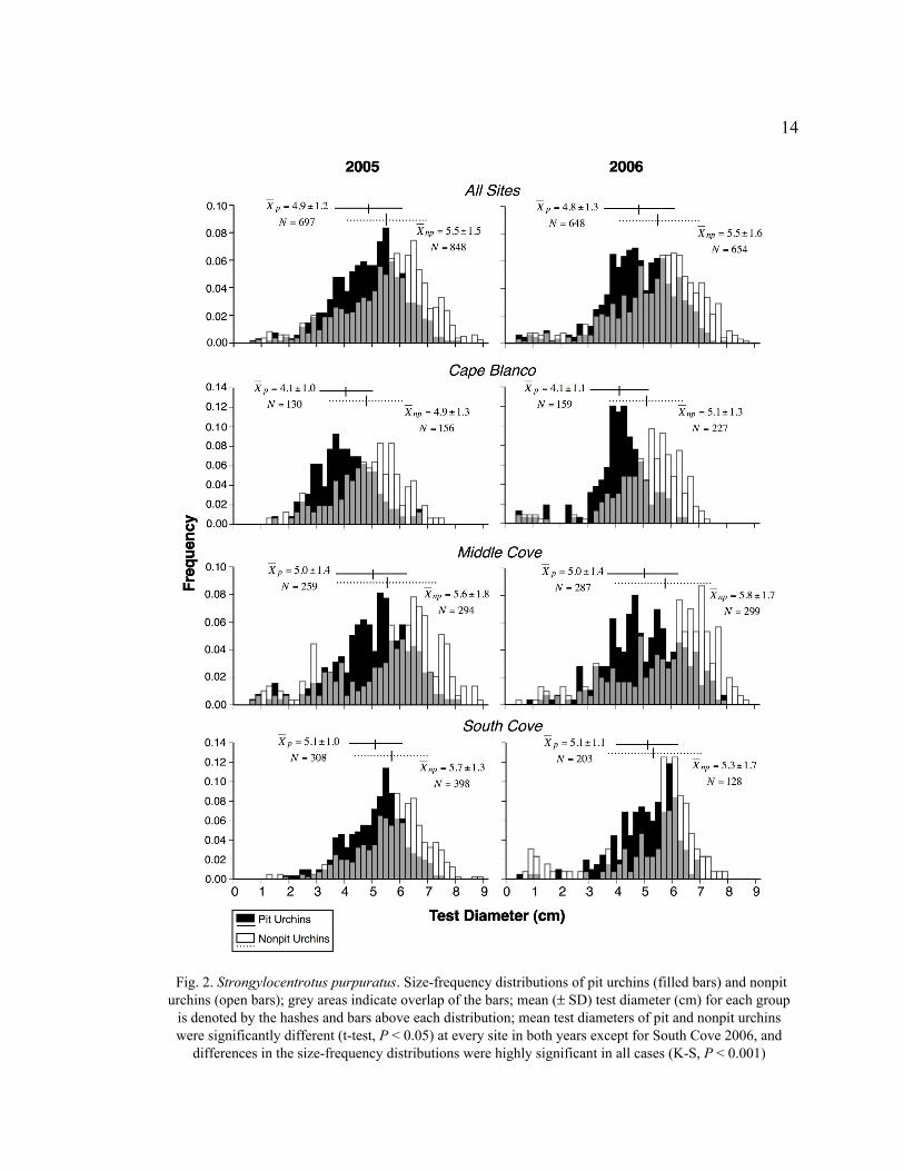
In 2005, 697 pit urchins and 848 pit urchins were sampled from eleven tidepools
at three sites. In 2006, 648 pit urchins and 654 nonpit urchins were collected and
measured from eleven different tidepools at the same three sites. All measurements are
contained in Appendix A. The data clearly show that Strongylocentrotus purpuratus
living outside pits had significantly larger diameters than those inside pits (t-test, P <
0.001). The mean (± SD) diameters of nonpit urchins and pit urchins from all sites and
sampling dates were 5.5 ± 1.6 cm and 4.9 ± 1.3 cm, respectively. This relationship was
found both in 2005 and 2006 (Fig. 2). At all but one site within a given year, S.
purpuratus was significantly larger when living outside pits (t-test, P < 0.001, Fig. 2). In
2006 at South Cove, nonpit urchins had a larger mean diameter than pit urchins, but the
difference was nonsignificant (t-test, P = 0.108). The difference between test diameters in
pit and nonpit urchins was greater at Cape Blanco than at Middle Cove or South Cove
(Fig. 2).
The size distribution of Strongylocentrotus purpuratus varied significantly
between microhabitats (K-S test, D = 0.260, P < 0.001). The size-frequency distributions
of pit and nonpit urchins were significantly different at every site in 2005 and 2006 (K-S
test, P < 0.001, Fig. 2). Histograms of nonpit urchins have similar shapes to those of pit
urchins, with the main difference being that distributions of nonpit urchins are shifted to
14
Fig. 2. Strongylocentrotus purpuratus. Size-frequency distributions of pit urchins (filled bars) and nonpit
urchins (open bars); grey areas indicate overlap of the bars; mean (± SD) test diameter (cm) for each group
is denoted by the hashes and bars above each distribution; mean test diameters of pit and nonpit urchins
were significantly different (t-test, P < 0.05) at every site in both years except for South Cove 2006, and
differences in the size-frequency distributions were highly significant in all cases (K-S, P < 0.001)
15
the right (larger) by about 1 cm. Purple sea urchins grow to about 1.5 cm in their first
year (Kenner 1992), so the individuals with test diameters <2 cm make up the recruitment
class for the year prior to sampling. Weak recruitment pulses were detected in 2005 and
2006 (Fig. 2), but neither abundance nor size distribution of recruits differed between
microhabitats (K-S, D = 0.196, P = 0.346). The size classes of recruits were similar in
both microhabitats, but overall, nonpit urchins were generally larger than pit urchins.
Thus, the size-frequency distributions of nonpit urchins were skewed to the left more than
pit urchins (Fig. 2).
The differences detected in test diameters and size-frequency distributions
between pit and nonpit urchins at large scales were also evident at the smaller scales of
tidepools (Table 1). Nonpit urchins had a larger test diameter than did pit urchins in 20 of
22 tidepools surveyed (exceptions were South Cove Tidepool B and Middle Cove
Tidepool G, of which only nine pit urchins were measured, so the sample mean probably
is not indicative of the population mean). Generally, there seemed to be a greater
microhabitat-based size difference at Cape Blanco than at South Cove or Middle Cove.
At Cape Blanco, nonpit urchins were significantly larger than pit urchins in five of eight
tidepools (Hochberg’s step-down sequential Bonferroni on Student’s t-test, P < 0.004).
The same can be said for only three of eight tidepools at Middle Cove and two of six
tidepools at South Cove. As with the overall site data, K-S tests were significant for most
(14 of 22) tidepools, indicating significant differences in population structure on a small
spatial scale (Hochberg’s Bonferroni, P < 0.004).
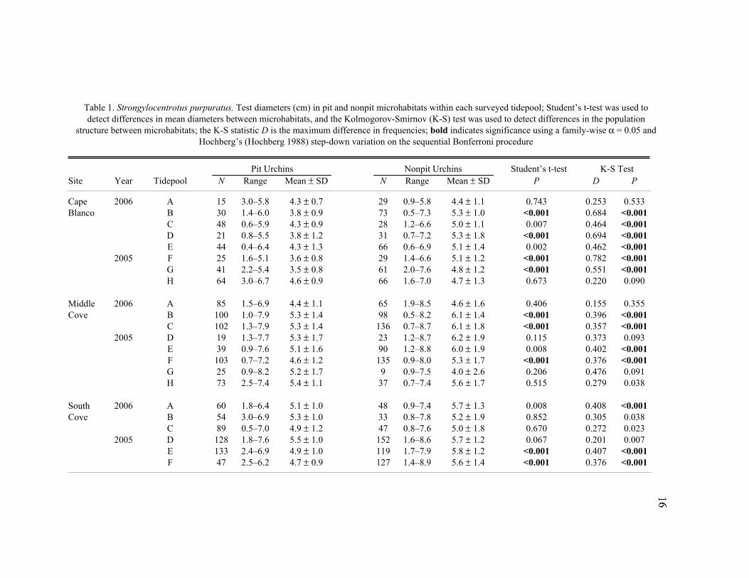
Table 1. Strongylocentrotus purpuratus. Test diameters (cm) in pit and nonpit microhabitats within each surveyed tidepool; Student’s t-test was used to
detect differences in mean diameters between microhabitats, and the Kolmogorov-Smirnov (K-S) test was used to detect differences in the population
structure between microhabitats; the K-S statistic D is the maximum difference in frequencies; bold indicates significance using a family-wise a = 0.05 and
Hochberg’s (Hochberg 1988) step-down variation on the sequential Bonferroni procedure
Pit Urchins Nonpit Urchins Student’s t-test K-S Test
Site Year Tidepool N Range Mean ± SD N Range Mean ± SD P D P
Cape 2006 A 15 3.0–5.8 4.3 ± 0.7 29 0.9–5.8 4.4 ± 1.1 0.743 0.253 0.533
Blanco B 30 1.4–6.0 3.8 ± 0.9 73 0.5–7.3 5.3 ± 1.0 <0.001 0.684 <0.001
C 48 0.6–5.9 4.3 ± 0.9 28 1.2–6.6 5.0 ± 1.1 0.007 0.464 <0.001
D 21 0.8–5.5 3.8 ± 1.2 31 0.7–7.2 5.3 ± 1.8 <0.001 0.694 <0.001
E 44 0.4–6.4 4.3 ± 1.3 66 0.6–6.9 5.1 ± 1.4 0.002 0.462 <0.001
2005 F 25 1.6–5.1 3.6 ± 0.8 29 1.4–6.6 5.1 ± 1.2 <0.001 0.782 <0.001
G 41 2.2–5.4 3.5 ± 0.8 61 2.0–7.6 4.8 ± 1.2 <0.001 0.551 <0.001
H 64 3.0–6.7 4.6 ± 0.9 66 1.6–7.0 4.7 ± 1.3 0.673 0.220 0.090
Middle 2006 A 85 1.5–6.9 4.4 ± 1.1 65 1.9–8.5 4.6 ± 1.6 0.406 0.155 0.355
Cove B 100 1.0–7.9 5.3 ± 1.4 98 0.5–8.2 6.1 ± 1.4 <0.001 0.396 <0.001
C 102 1.3–7.9 5.3 ± 1.4 136 0.7–8.7 6.1 ± 1.8 <0.001 0.357 <0.001
2005 D 19 1.3–7.7 5.3 ± 1.7 23 1.2–8.7 6.2 ± 1.9 0.115 0.373 0.093
E 39 0.9–7.6 5.1 ± 1.6 90 1.2–8.8 6.0 ± 1.9 0.008 0.402 <0.001
F 103 0.7–7.2 4.6 ± 1.2 135 0.9–8.0 5.3 ± 1.7 <0.001 0.376 <0.001
G 25 0.9–8.2 5.2 ± 1.7 9 0.9–7.5 4.0 ± 2.6 0.206 0.476 0.091
H 73 2.5–7.4 5.4 ± 1.1 37 0.7–7.4 5.6 ± 1.7 0.515 0.279 0.038
South 2006 A 60 1.8–6.4 5.1 ± 1.0 48 0.9–7.4 5.7 ± 1.3 0.008 0.408 <0.001
Cove B 54 3.0–6.9 5.3 ± 1.0 33 0.8–7.8 5.2 ± 1.9 0.852 0.305 0.038
C 89 0.5–7.0 4.9 ± 1.2 47 0.8–7.6 5.0 ± 1.8 0.670 0.272 0.023
2005 D 128 1.8–7.6 5.5 ± 1.0 152 1.6–8.6 5.7 ± 1.2 0.067 0.201 0.007
E 133 2.4–6.9 4.9 ± 1.0 119 1.7–7.9 5.8 ± 1.2 <0.001 0.407 <0.001
F 47 2.5–6.2 4.7 ± 0.9 127 1.4–8.9 5.6 ± 1.4 <0.001 0.376 <0.001

17
Morphological Differences
ANCOVA with wet mass as a covariate
The morphology of Strongylocentrotus purpuratus varied significantly between
microhabitats for two of the eleven parameters investigated (test height, mass of skeletal
components), and microhabitat interactions were significant in three other parameters
(test diameter, spine length, jaw length) (ANCOVA, P < 0.05, Table 2). Differences in
Table 2. Resulting adjusted means (± SD) for sea urchin morphological parameters in a three-way partially
nested mixed model ANCOVA with total wet mass (88.65 g) as the covariate; the random factor tidepool is
nested within the random factor site, and microhabitat is fixed; units are centimeters and grams unless
otherwise stated; * Microhabitat effect P < 0.05; ** Microhabitat x site interaction P < 0.05; ***
Microhabitat x tidepool (site) interaction P < 0.05; a
compression strength violated the assumption of
homogenous slopes and was not analyzed in the ANCOVA model
Parameter Pit Urchins Nonpit Urchins
Diameter 5.6 ± 0.2 ** 5.7 ± 0.2
Height 3.0 ± 0.2 * 2.9 ± 0.2
Height:Diameter (h/d) 0.54 ± 0.04 0.51 ± 0.04
Peristomial diameter 1.92 ± 0.09 1.90 ± 0.09
Mass of:
Gonad 8.38 ± 2.52 8.19 ± 2.52
Gut 8.28 ± 2.06 7.98 ± 2.06
Aristotle’s lantern 2.50 ± 0.37 2.31 ± 0.37
Skeletal components 44.57 ± 2.80 * 46.47 ± 2.80
Spine length 0.92 ± 0.13 ** 1.03 ± 0.13
Jaw length 1.38 ± 0.08 *** 1.32 ± 0.08
Test thickness (mm) 1.14 ± 0.09 1.17 ± 0.09a Compression strength (kg) 41.5 ± 10.5 41.0 ± 10.5
18
the remaining parameters were explained by variation at the tidepool and site levels. The
average total wet mass (the covariate) of the 169 purple sea urchins included in the
analysis was 88.65 g. Data for all 180 collected sea urchins can be found in Appendix B.
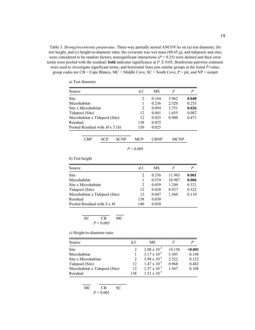
The ANCOVA for test diameter showed a significant interaction between site and
microhabitat (F2,150 = 3.751, P = 0.026, Table 3a). The adjusted mean (± SD) test
diameter (cm) of Cape Blanco pit urchins (5.6 ± 0.2) was significantly less than for
Middle Cove pit urchins, Cape Blanco nonpit urchins, and Middle Cove nonpit urchins
(all groups: 5.7 ± 0.2, P < 0.001). No significant differences in test diameter were
detected between microhabitats at Middle Cove or South Cove.
Test height was significantly different between microhabitats (ANCOVA, F1,12 =
10.987, P = 0.006, Table 3b) and sites (ANCOVA, F2,12 = 11.983, P = 0.001). Pit urchins
were taller than nonpit urchins, with an adjusted mean (± SD) test height (cm) of 3.0 ±
0.2 compared with 2.9 ± 0.2. Site effects were driven by shorter test heights at Middle
Cove relative to Cape Blanco (P = 0.001) and South Cove (P < 0.001).
The h/d ratio was significantly different between sites (ANCOVA, F2,12 = 14.156,
P < 0.001, Table 3c); urchins at Middle Cove had a significantly smaller mean (± SD) h/d
ratio (0.499 ± 0.039) than South Cove (0.535 ± 0.039, P < 0.001) or Cape Blanco (0.531
± 0.039, P < 0.001). Pit urchins (0.535 ± 0.039) had a larger h/d ratio than nonpit urchins
(0.508 ± 0.039) but the difference was not significant (P = 0.148).
19
Table 3. Strongylocentrotus purpuratus. Three-way partially nested ANCOVAs on (a) test diameter, (b)
test height, and (c) height-to-diameter ratio; the covariate was wet mass (88.65 g), and tidepools and sites
were considered to be random factors; nonsignificant interactions (P > 0.25) were deleted and their error
terms were pooled with the residual; bold indicates significance at P
�
£ 0.05; Bonferroni pairwise contrasts
were used to investigate significant terms, and horizontal lines join similar groups at the listed P-value;
group codes are CB = Cape Blanco, MC = Middle Cove, SC = South Cove, P = pit, and NP = nonpit
a) Test diameter
Source d.f. MS F P
Site 2 0.164 3.962 0.048
Microhabitat 1 0.236 2.520 0.253
Site x Microhabitat 2 0.094 3.751 0.026
Tidepool (Site) 12 0.041 1.655 0.082
Microhabitat x Tidepool (Site) 12 0.025 0.980 0.471
Residual 138 0.025
Pooled Residual with M x T (S) 150 0.025
CBP SCP SCNP MCP CBNP MCNP
P < 0.005
b) Test height
Source d.f. MS F P
Site 2 0.336 11.983 0.001
Microhabitat 1 0.519 10.987 0.006
Site x Microhabitat 2 0.059 1.249 0.321
Tidepool (Site) 12 0.028 0.927 0.522
Microhabitat x Tidepool (Site) 12 0.047 1.560 0.110
Residual 138 0.030
Pooled Residual with S x M 140 0.030
SC CB MC
P < 0.005
c) Height-to-diameter ratio
Source d.f. MS F P
Site 2 2.08 x 10⁻²
14.156 <0.001
Microhabitat 1 3.17 x 10⁻²
5.303 0.148
Site x Microhabitat 2 5.98 x 10⁻³
2.522 0.122
Tidepool (Site) 12 1.47 x 10⁻³
0.968 0.482
Microhabitat x Tidepool (Site) 12 2.37 x 10⁻³
1.567 0.108
Residual 138 1.51 x 10⁻³
MC CB SC
P < 0.001

20
Microhabitat significantly affected the mass of skeletal components (ANCOVA,
F1,12 = 14.975, P = 0.002, Table 4a). Nonpit urchins with an adjusted mass of 88.65 g
contained skeletal components with a mean (± SD) of 46.45 ± 2.80 g (52.4%) compared
to only 44.57 ± 2.80 g (50.3%) in pit urchins. Urchins from different sites (P > 0.85) and
tidepools (P > 0.35) had similar skeletal masses. The microhabitat-based difference in
skeletal mass may be related to spine length, for which the interaction between site and
microhabitat was significant (ANCOVA, F2,150 = 9.809, P < 0.001, Table 4b). Spines of
nonpit urchins were significantly (P < 0.001) longer than spines of pit urchins both at
Middle Cove (difference of 0.23 cm, 23% longer) and at Cape Blanco (difference of 0.10
cm, 12% longer). The spines of Middle Cove nonpit urchins were significantly longer
than the spines of urchins in either microhabitat at any site (P < 0.001). At South Cove,
there was no significant difference in spine length between pit urchins and nonpit urchins.
The variability in jaw length in Strongylocentrotus purpuratus was explained by a
significant (ANCOVA, F12,150 = 2.082, P = 0.022, Table 4c) interaction between
microhabitat and tidepool. Although pit urchins consistently contained larger jaws than
nonpit urchins, the relationship was reversed in three of fifteen tidepools (one at Cape
Blanco and two at South Cove). The resulting Site x Microhabitat interaction masked a
real effect, which was investigated with a Bonferroni pairwise comparison. Within
Middle Cove (P = 0.028) and Cape Blanco (P < 0.001), the jaw lengths of pit urchins
were significantly greater than nonpit urchins.
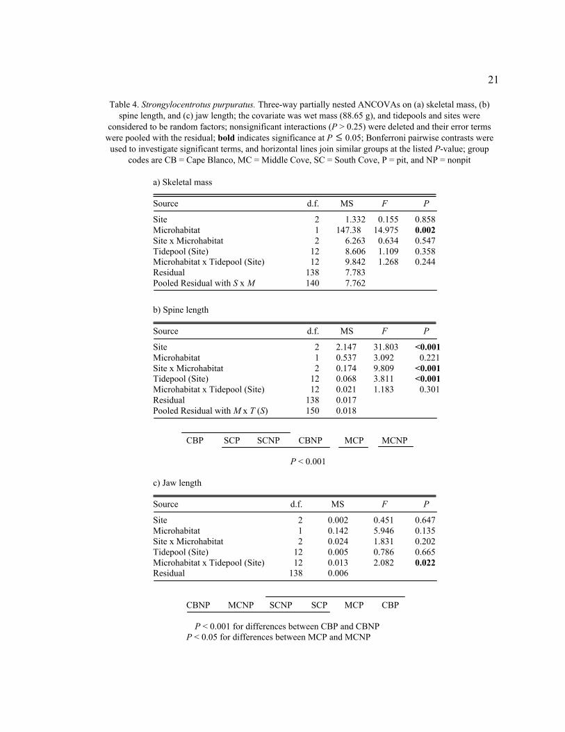
21
Table 4. Strongylocentrotus purpuratus. Three-way partially nested ANCOVAs on (a) skeletal mass, (b)
spine length, and (c) jaw length; the covariate was wet mass (88.65 g), and tidepools and sites were
considered to be random factors; nonsignificant interactions (P > 0.25) were deleted and their error terms
were pooled with the residual; bold indicates significance at P
�
£ 0.05; Bonferroni pairwise contrasts were
used to investigate significant terms, and horizontal lines join similar groups at the listed P-value; group
codes are CB = Cape Blanco, MC = Middle Cove, SC = South Cove, P = pit, and NP = nonpit
a) Skeletal mass
Source d.f. MS F P
Site 2 1.332 0.155 0.858
Microhabitat 1 147.38 14.975 0.002
Site x Microhabitat 2 6.263 0.634 0.547
Tidepool (Site) 12 8.606 1.109 0.358
Microhabitat x Tidepool (Site) 12 9.842 1.268 0.244
Residual 138 7.783
Pooled Residual with S x M 140 7.762
b) Spine length
Source d.f. MS F P
Site 2 2.147 31.803 <0.001
Microhabitat 1 0.537 3.092 0.221
Site x Microhabitat 2 0.174 9.809 <0.001
Tidepool (Site) 12 0.068 3.811 <0.001
Microhabitat x Tidepool (Site) 12 0.021 1.183 0.301
Residual 138 0.017
Pooled Residual with M x T (S) 150 0.018
CBP SCP SCNP CBNP MCP MCNP
P < 0.001
c) Jaw length
Source d.f. MS F P
Site 2 0.002 0.451 0.647
Microhabitat 1 0.142 5.946 0.135
Site x Microhabitat 2 0.024 1.831 0.202
Tidepool (Site) 12 0.005 0.786 0.665
Microhabitat x Tidepool (Site) 12 0.013 2.082 0.022
Residual 138 0.006
CBNP MCNP SCNP SCP MCP CBP
P < 0.001 for differences between CBP and CBNP
P < 0.05 for differences between MCP and MCNP

22
Although microhabitat was not a significant contributor to the variability in the
remaining measured parameters, site and tidepool were. The gut and gonad masses were
quite variable, and the Microhabitat x Tidepool (Site) interactions were significant
(ANCOVA, gut mass: F12,140 = 2.77, P = 0.002, Table 5a; gonad mass: F12,140 = 2.33, P =
0.010, Table 5b). Pit urchins at Middle Cove appeared to have much heavier guts and
lighter gonads than pit urchins at South Cove and Cape Blanco, but significant
interactions prevented post-hoc testing.
The Microhabitat x Tidepool (Site) interaction was also significant for the mass of
the Aristotle’s lantern (ANCOVA, F12,138 = 3.50, P < 0.001, Table 5c). Like jaw length,
lantern mass was greater in pit urchins than in nonpit urchins for most, but not all
tidepools. Peristomial diameter (ANCOVA, F12,140 = 2.58, P = 0.004, Table 6a) and test
thickness (ANCOVA, F12,140 = 2.20, P = 0.027, Table 6b) were significantly different
among tidepools, and the latter was significantly different (ANCOVA, F2,12 = 6.68, P =
0.011, Table 6b) among sites, but not microhabitats.
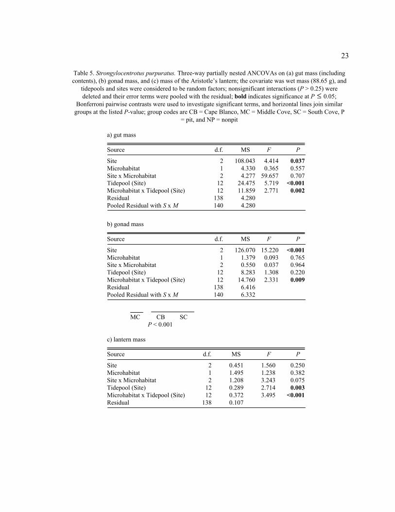
23
Table 5. Strongylocentrotus purpuratus. Three-way partially nested ANCOVAs on (a) gut mass (including
contents), (b) gonad mass, and (c) mass of the Aristotle’s lantern; the covariate was wet mass (88.65 g), and
tidepools and sites were considered to be random factors; nonsignificant interactions (P > 0.25) were
deleted and their error terms were pooled with the residual; bold indicates significance at P
�
£ 0.05;
Bonferroni pairwise contrasts were used to investigate significant terms, and horizontal lines join similar
groups at the listed P-value; group codes are CB = Cape Blanco, MC = Middle Cove, SC = South Cove, P
= pit, and NP = nonpit
a) gut mass
Source d.f. MS F P
Site 2 108.043 4.414 0.037
Microhabitat 1 4.330 0.365 0.557
Site x Microhabitat 2 4.277 59.657 0.707
Tidepool (Site) 12 24.475 5.719 <0.001
Microhabitat x Tidepool (Site) 12 11.859 2.771 0.002
Residual 138 4.280
Pooled Residual with S x M 140 4.280
b) gonad mass
Source d.f. MS F P
Site 2 126.070 15.220 <0.001
Microhabitat 1 1.379 0.093 0.765
Site x Microhabitat 2 0.550 0.037 0.964
Tidepool (Site) 12 8.283 1.308 0.220
Microhabitat x Tidepool (Site) 12 14.760 2.331 0.009
Residual 138 6.416
Pooled Residual with S x M 140 6.332
MC CB SC
P < 0.001
c) lantern mass
Source d.f. MS F P
Site 2 0.451 1.560 0.250
Microhabitat 1 1.495 1.238 0.382
Site x Microhabitat 2 1.208 3.243 0.075
Tidepool (Site) 12 0.289 2.714 0.003
Microhabitat x Tidepool (Site) 12 0.372 3.495 <0.001
Residual 138 0.107

24
Table 6. Strongylocentrotus purpuratus. Three-way partially nested ANCOVAs on (a) peristomial diameter
and (b) test thickness; the covariate was wet mass (88.65 g), and tidepools and sites were considered to be
random factors; nonsignificant interactions (P > 0.25) were deleted and their error terms were pooled with
the residual; bold indicates significance at P
�
£ 0.05; Bonferroni pairwise contrasts were used to investigate
significant terms, and horizontal lines join similar groups at the listed P-value; group codes are CB = Cape
Blanco, MC = Middle Cove, SC = South Cove, P = pit, and NP = nonpit
a) peristomial diameter
Source d.f. MS F P
Site 2 0.052 3.112 0.082
Microhabitat 1 0.021 2.046 0.178
Site x Microhabitat 2 0.003 0.272 0.766
Tidepool (Site) 12 0.017 2.584 0.004
Microhabitat x Tidepool (Site) 12 0.010 1.630 0.090
Residual 138 0.006
Pooled Residual with S x M 140 0.006
b) test thickness
Source d.f. MS F P
Site 2 2.09x10⁻³
6.677 0.011
Microhabitat 1 3.90x10⁻⁴
1.868 0.197
Site x Microhabitat 2 4.0x10⁻⁵
0.191 0.829
Tidepool (Site) 12 3.13x10⁻⁴
2.020 0.027
Microhabitat x Tidepool (Site) 12 2.09x10⁻⁴
1.348 0.198
Residual 138 1.60x10⁻⁴
Pooled Residual with S x M 140 1.55x10⁻⁴
CB SC MC
P < 0.05
ANCOVA with test diameter as a covariate
Using the data for all sea urchins with test diameter as a covariate yields slightly
different results. A three-way ANCOVA was not used to test ln (test height) because of a
significant interaction. Small Strongylocentrotus purpuratus at Cape Blanco had large
test heights, but large S. purpuratus had small test heights relative to Middle Cove and
25
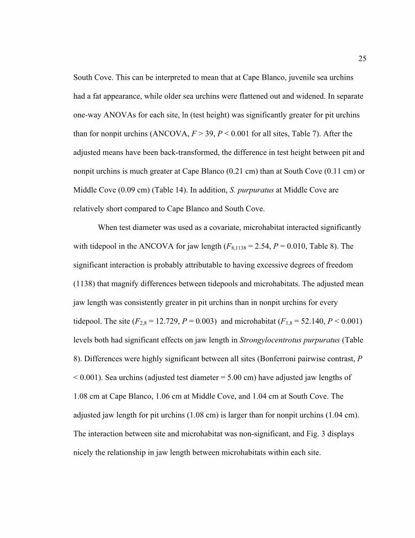
South Cove. This can be interpreted to mean that at Cape Blanco, juvenile sea urchins
had a fat appearance, while older sea urchins were flattened out and widened. In separate
one-way ANOVAs for each site, ln (test height) was significantly greater for pit urchins
than for nonpit urchins (ANCOVA, F > 39, P < 0.001 for all sites, Table 7). After the
adjusted means have been back-transformed, the difference in test height between pit and
nonpit urchins is much greater at Cape Blanco (0.21 cm) than at South Cove (0.11 cm) or
Middle Cove (0.09 cm) (Table 14). In addition, S. purpuratus at Middle Cove are
relatively short compared to Cape Blanco and South Cove.
When test diameter was used as a covariate, microhabitat interacted significantly
with tidepool in the ANCOVA for jaw length (F8,1138 = 2.54, P = 0.010, Table 8). The
significant interaction is probably attributable to having excessive degrees of freedom
(1138) that magnify differences between tidepools and microhabitats. The adjusted mean
jaw length was consistently greater in pit urchins than in nonpit urchins for every
tidepool. The site (F2,8 = 12.729, P = 0.003) and microhabitat (F1,8 = 52.140, P < 0.001)
levels both had significant effects on jaw length in Strongylocentrotus purpuratus (Table
8). Differences were highly significant between all sites (Bonferroni pairwise contrast, P
< 0.001). Sea urchins (adjusted test diameter = 5.00 cm) have adjusted jaw lengths of
1.08 cm at Cape Blanco, 1.06 cm at Middle Cove, and 1.04 cm at South Cove. The
adjusted jaw length for pit urchins (1.08 cm) is larger than for nonpit urchins (1.04 cm).
The interaction between site and microhabitat was non-significant, and Fig. 3 displays
nicely the relationship in jaw length between microhabitats within each site.
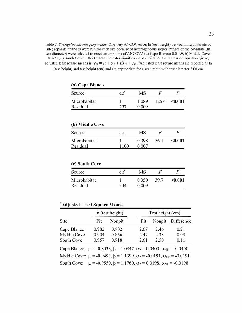
26
Table 7. Strongylocentrotus purpuratus. One-way ANCOVAs on ln (test height) between microhabitats by
site; separate analyses were run for each site because of heterogeneous slopes; ranges of the covariate (ln
test diameter) were selected to meet assumptions of ANCOVA: a) Cape Blanco: 0.0-1.9, b) Middle Cove:
0.0-2.1, c) South Cove: 1.0-2.0; bold indicates significance at P
�
£ 0.05; the regression equation giving
adjusted least square means is
�
yij = m + a i + bxij + e ij ; aAdjusted least square means are reported as ln
(test height) and test height (cm) and are appropriate for a sea urchin with test diameter 5.00 cm
(a) Cape Blanco
Source d.f. MS F P
Microhabitat 1 1.089 126.4 <0.001
Residual 757 0.009
(b) Middle Cove
Source d.f. MS F P
Microhabitat 1 0.398 56.1 <0.001
Residual 1100 0.007
(c) South Cove
Source d.f. MS F P
Microhabitat 1 0.350 39.7 <0.001
Residual 944 0.009
aAdjusted Least Square Means
ln (test height) Test height (cm)
Site Pit Nonpit Pit Nonpit Difference
Cape Blanco 0.982 0.902 2.67 2.46 0.21
Middle Cove 0.904 0.866 2.47 2.38 0.09
South Cove 0.957 0.918 2.61 2.50 0.11
Cape Blanco: m = -0.8038, b = 1.0847, aP = 0.0400, aNP = -0.0400
Middle Cove: m = -0.9493, b = 1.1399, aP = -0.0191, aNP = -0.0191
South Cove: m = -0.9550, b = 1.1760, aP = 0.0198, aNP = -0.0198
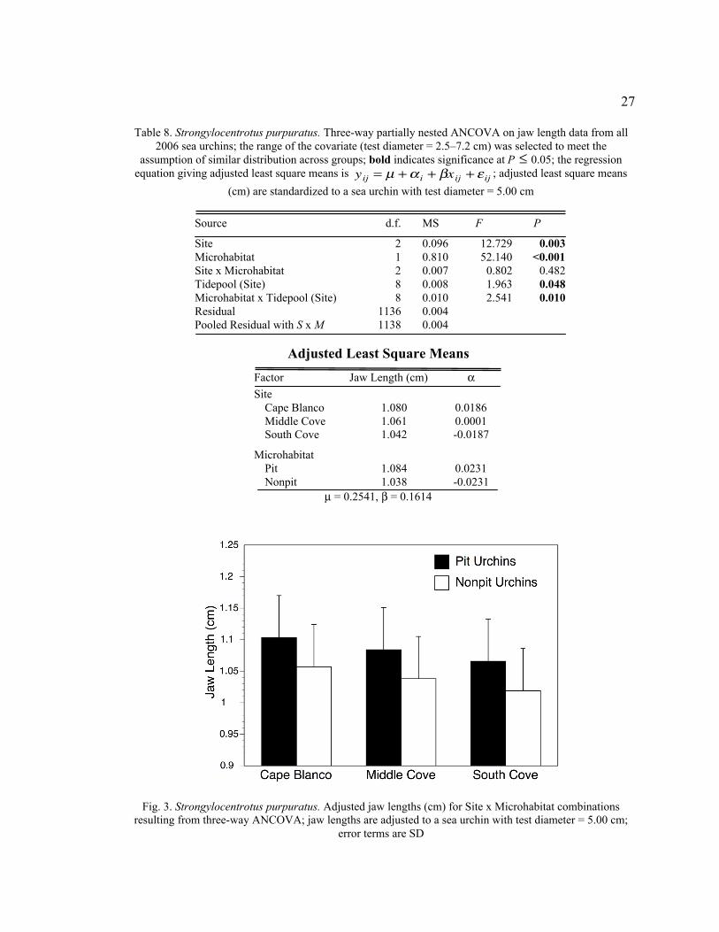
27
Table 8. Strongylocentrotus purpuratus. Three-way partially nested ANCOVA on jaw length data from all
2006 sea urchins; the range of the covariate (test diameter = 2.5–7.2 cm) was selected to meet the
assumption of similar distribution across groups; bold indicates significance at P
�
£ 0.05; the regression
equation giving adjusted least square means is
�
yij = m + a i + bxij + e ij ; adjusted least square means
(cm) are standardized to a sea urchin with test diameter = 5.00 cm
Source d.f. MS F P
Site 2 0.096 12.729 0.003
Microhabitat 1 0.810 52.140 <0.001
Site x Microhabitat 2 0.007 0.802 0.482
Tidepool (Site) 8 0.008 1.963 0.048
Microhabitat x Tidepool (Site) 8 0.010 2.541 0.010
Residual 1136 0.004
Pooled Residual with S x M 1138 0.004
Adjusted Least Square Means
Factor Jaw Length (cm) a
Site
Cape Blanco 1.080 0.0186
Middle Cove 1.061 0.0001
South Cove 1.042 -0.0187
Microhabitat
Pit 1.084 0.0231
Nonpit 1.038 -0.0231
m = 0.2541, b = 0.1614
Fig. 3. Strongylocentrotus purpuratus. Adjusted jaw lengths (cm) for Site x Microhabitat combinations
resulting from three-way ANCOVA; jaw lengths are adjusted to a sea urchin with test diameter = 5.00 cm;
error terms are SD

28
DISCUSSION
This study used field-sampling techniques at three locations on the Oregon coast
to test for demographic and morphological differences in Strongylocentrotus purpuratus
living inside and outside pits. The null hypotheses that the population structure and mean
test diameter did not vary between microhabitats were rejected. Microhabitat-based size-
frequency distributions were dissimilar within every site and most tidepools, and nonpit
urchins were significantly larger than pit urchins. The null hypothesis that pit urchins
were not morphologically different from nonpit urchins was also rejected. Purple sea
urchins living inside pits had relatively taller test heights, larger jaws, shorter spines, and
less skeletal mass than those living in the same tidepools but outside pits.
Morphological differences indicate microhabitat fidelity
I found distinct morphological differences in Strongylocentrotus purpuratus from
adjacent microhabitats. Is this due to morphological plasticity, with pit urchins and nonpit
urchins within centimeters of each other altering their morphology in response to
different suites of forces? Plasticity in sea urchins, though widely examined (Ebert 1996)
has rarely, if ever been described over such small scales. Rogers-Bennett et al. (1995)
found morphological differences in a population of S. franciscanus, in which sea urchins
living at 5-m depth (incidentally in rock “bowls”) had shorter spines, larger gonads,
thicker tests, and smaller Aristotle’s lanterns than those living at 14- or 23-m depth. In
29
the western Pacific, the sea urchin Anthocidaris crassispina sometimes inhabits pits
created by the sea urchin Echinostrephus aciculatus. Yusa and Yamamoto (1994) found
that A. crassispina in pits had three times heavier gonads than individuals outside pits,
though the groups also came from two separate tidepools. Despite the presence of
morphological differences on the scales of meters and tens of meters, the effects of
smaller scales remain largely unexplored. This study indicates that the microhabitat scale
does influence the morphology of S. purpuratus in significant ways.
The observed morphological differences of Strongylocentrotus purpuratus living
inside and outside pits imply some degree of microhabitat fidelity in individuals. If sea
urchins were frequent movers within tidepools, one would not expect pit and nonpit
urchins to exhibit distinct forms. This possible lack of movement provides a partial
explanation for microhabitat-based differences in jaw size. Morphological plasticity in
sea urchins is often attributed to food availability [eg. Strongylocentrotus purpuratus
(Ebert 1980), S. droebachiensis (Minor & Scheibling 1997), Diadema antillaum (Levitan
1991), Echinometra mathaei (Black et al. 1984), and Paracentrotus lividus (Fernandez &
Boudouresque 1997)]. Sea urchins with little or no food continue to allocate resources to
the Aristotle’s lantern, making it relatively large compared to well-fed urchins. The larger
relative jaw sizes I observed in pit urchins may be due to food limitation. Pit and nonpit
urchins occurred in the same tidepools, so why would just one group be food limited?
Purple sea urchins in the intertidal tend to be sedentary feeders; drifting algae is trapped
by their spines or grabbed by their tube feet (Ebert 1968, Dayton 1975). Pit urchins
might be at a disadvantage if their pit is so deep they have difficulty reaching out of it for
30
food. Sedentary sea urchins that do not leave their pits to forage might become food
limited.
Other microhabitat-based differences in morphology would not seem to be related
to food resources. The relatively short spines of pit urchins at two of three sites suggest
that rubbing against the sides of pits wore down their spines. Qualitative field
observations indicated that the spines on pit urchins sometimes lack epithelial tissue at
the tip and are not as sharp as those on nonpit urchins. That all sea urchins at South Cove
had short spines, regardless of microhabitat, is perhaps related to site characteristics.
South Cove has much more loose cobble than Middle Cove or Cape Blanco. Here, many
sea urchins exhibited a covering behavior in which they held pieces of cobble with their
tube feet on top of their test. When waves are breaking on the intertidal habitat, cobble
that is held by a sea urchin or loose in a tidepool might rub against or break spines,
leading to smaller length spines.
The greater skeletal mass in nonpit urchins is probably not due to their longer
spines because the trend is not constant among all three sites. Water velocity and
hydrodynamic forces experienced by a sea urchin might affect the thickness of its test. In
the absence of protective pits, physical exposure might induce nonpit urchins to allocate
more resources to their skeleton (Lewis & Storey 1984, Rogers-Bennett et al. 1995). An
alternative possibility is that differences in test shape led to heavier skeletal components
in nonpit urchins. Pit urchins tend to be relatively taller and more compact while nonpit
urchins tend to be shorter and wider, leading to significant differences in h/d ratio. At all
sites, pit urchins had a greater h/d ratio than nonpit urchins. Just as a spherical object

31
contains less surface area than a pancake-shaped object with the same volume, a tall pit
urchin might require less skeletal material than a short nonpit urchin of similar mass.
How could a sea urchin’s microhabitat affect its shape? The shape of sea urchins
has been compared to that of a water droplet; in both, structurally sound forms are created
by balancing internal pressure forces (Ellers 1993). In sea urchins, changes in any of the
internal pressures (weight, podial forces, coelomic pressure) could alter the forces exerted
on the test. The force most likely to be affected by living inside a pit microhabitat is that
imposed by the podia as they cling to the substratum. An urchin on a flat surface holds
itself in place with its oral podia, creating a downward force. An urchin inside a
depression, however, could reduce this downward pull by podia by attaching to the sides
of the pit with additional podia. Furthermore, a sea urchin will often wedge its spines
against the sides of a pit to hold itself in place, creating an inward force on the side of the
test. In pit urchins, perhaps the diminished use of oral podia and the forces created by
jamming spines against the rock alter internal pressure forces. These changes in internal
forces and the inherent flexibility in sutures between test plates (Johnson et al. 2002)
could cause the tests of pit urchins to deviate from the typical water droplet shape.
Nonpit urchins tend to be larger than pit urchins
Strongylocentrotus purpuratus, an echinoid that is ecologically important and
common along the North American West coast, has been the subject of numerous
population structure studies. The sea urchin populations investigated in this study were
32
similar in size structure to those sampled in 1985 at Cape Blanco and Sunset Bay,
Oregon, about five km north of Cape Arago (Ebert & Russell 1988). In both studies, sea
urchins with test diameters of 3–8 cm made up the bulk of the population, as recruitment
was relatively rare. Ebert (1968) observed similar patterns from 1964–1967 at Sunset Bay
with one year of exceptional recruitment in 1963, the only such event over more than two
decades (Ebert & Russell 1988). In a latitudinal study, Ebert and Russell (1988) found
that at all but one site in California, populations of S. purpuratus had smaller mean test
diameters than those inside or outside pits in this study. Although pit urchins investigated
in the study reported here were significantly smaller than nonpit urchins, the urchins I
studied had a larger mean test size than has been observed with most intertidal
populations of purple sea urchins.
The present study found clear size structure differences in purple sea urchins
between different microhabitats. There is no strict definition for microhabitat, leaving
researchers to define it as they see fit. For this research, I have defined microhabitats as
the smallest scale at which physical or chemical variables that are relevant to the
organism differ (Morris 1987). In the case of pits, hydrodynamic forces certainly are
altered relative to a nonpit microhabitat. When the classification of microhabitat is
expanded beyond that employed in this study, microhabitat boundaries might be defined
by tidepools or substratum rather than microtopography. Using this expanded definition,
more studies can speak to the potential impacts of spatial scales smaller than sites on sea
urchin population structure. In South Africa, Drummond (1993) investigated the size
structure of the sea urchin Stomopneustes variolaris in three intertidal areas on the same

33
beach. She found distinct differences in mean size, and the smallest urchins were on an
intertidal shelf in which they inhabited “small hollows.” Ebert (1968) also observed size
differences in purple sea urchins living in different portions of the same bay, but he
attributed them to varying food availability. Growth in Strongylocentrotus purpuratus
varies among tidepools such that growth rates in pools thousands of kilometers apart
might be more similar than between two at the same site (Russell 1987). In Norway,
Sivertsen & Hopkins (1995) found large green sea urchins (S. droebachiensis) in barrens
and kelp beds while smaller urchins dominated areas where the substratum was rocky,
shelly, or covered with coralline algae. Unfortunately, data were collected and pooled in a
way that prevents determining whether differences among dates, sites, or substrata were
related to the observed differences in S. droebachiensis. Still, these studies lend evidence
to the idea that spatial scales smaller than entire sites can affect the demography of sea
urchins. The present study demonstrates that scales smaller than those previously
investigated can also affect size structure in S. purpuratus.
In Strongylocentrotus purpuratus, the microhabitat-based difference in size
structure does not seem to apply to juvenile sea urchins. Visual inspection of Fig. 2.
reveals that recently recruited (
�
£2 cm) S. purpuratus did not seem to prefer pit or nonpit
microhabitats. When recruits were found in either microhabitat, they were usually
beneath the spines of conspecifics (Tegner & Dayton 1981, Nishizaki & Ackerman
2001). Small urchins were occasionally found in similarly sized pits, and some small
urchins, in the absence of adults, were found attached to clumps of coralline red algae.
Since most small sea urchins were found beneath adults, the choice of microhabitat of the

34
adult tended to define the microhabitat inhabited by recruits. Only small recruitment
pulses were detected during the study, so it would be worthwhile to investigate juvenile
microhabitat following heavy recruitment.
At Middle Cove and South Cove, about 90% of the largest purple urchins (
�
!7.5
cm) were found outside pits. At Cape Blanco, where the mean test diameter was smaller,
almost all of the urchins
�
!6 cm were found outside pits. Drummond (1993) described
larger sea urchin burrows in sandstone than in a harder substratum, and she proposed that
it was easier for urchins to dig large cavities from the softer material. Sea urchins wear
away the insides of pits by biting pieces of rock with their Aristotle’s lantern and
scraping the sides with their spines. Most of the bedrock at Cape Arago, including Middle
and South Cove’s, is relatively soft sedimentary sandstone. Purple urchins have
excavated large, hemispherical pits that can exceed 7 cm in diameter. The metamorphic
basalt at Cape Blanco is much harder than sandstone and may limit the bio-erosive
capabilities of purple sea urchins.
How can the differences in the population structure of Strongylocentrotus
purpuratus between microhabitats be explained?
Several hypotheses may explain the difference in size between purple sea urchins
inside and outside pits. The separate distributions might be the result of variation in
growth; nonpit urchins may grow faster than pit urchins (see Chapter III). Growth could
be reduced in two ways. First, the sides of a pit may constrain the growth of its
inhabitant. Most pit urchins nearly fill their cavity with little room to spare. Could growth
35
be more difficult or even impossible for a sea urchin closed in on all sides? If an urchin
constricted in a pit is to grow, it might be forced to grow upward, which would help
explain the larger h/d ratio in pit urchins. Second, a reduced growth hypothesis could be
explained by differences in food availability between microhabitats. Since S. purpuratus
is essentially a sedentary feeder of drift algae, it is possible that more food is accessible to
exposed, nonpit sea urchins, which could lead to increased growth rates and larger test
diameters. Studies have demonstrated that echinoid populations can display differential
growth rates within a site (Ebert 1968, Rowley 1990, Vadas et al. 2002), so it is plausible
that the microhabitat scale could also affect growth. Spine damage incurs repair costs that
reduce growth in sea urchins (Ebert 1968), and the shorter spines of pit urchins at two
sites indicate that they may experience a higher rate of damage (possibly from scraping
the sides of the pit) than nonpit urchins.
A second hypothesis for the observed size-frequency distributions is that pit
urchins tend to move between microhabitats as they age (Chapter IV). When sea urchins
are smaller, they can inhabit a pit and still have plenty of room for growth. At this stage,
the protection of a pit might make it a preferred habitat. In Fiji, sea urchins (Echinometra
sp.) occur on the crests and flats of reef atolls; crests are much more wave-exposed, but
they contain small protective crevices. Appana et al. (2004) found that urchins on the
crests of reefs had much smaller mean test diameters than those inhabiting reef flats.
They suggested that either larger sea urchins avoid areas of high wave exposure to protect
their spines, or predation pressure differs between the two habitats. Movement tends to be
rare in recruits of Strongylocentrotus droebachiensis, which remain cryptically hidden for
36
the early part of their life (Dumont et al. 2004). Both of these studies cite the need for
protection as a reason that smaller urchins might inhabit a hole or crevice until they are
better suited to deal with environmental pressures.
However, a sedentary pit urchin will eventually be faced with the dilemma that it
cannot erode its pit as fast as it can grow. The cost of remaining in a pit would be the
inhibition of growth. Since gonad mass increases with whole body mass, the cessation of
growth could be a major disadvantage to a sea urchin. By changing from a pit to a non-pit
microhabitat, this inhibition of growth could be avoided, allowing the sea urchin’s body
and gonads to continue increasing in size. Very large nonpit urchins have test diameters
of 8 cm, about 1 cm greater than the largest pit urchins, translating to a nearly 50% larger
total mass [for S. purpuratus: m =
�
(0.95* d2* h) /1140 , R
2 = 0.983 where m is mass (g), d
is test diameter (cm), and h is test height (cm)]. Some large sea urchins, however, have
not moved out of their pits. If the nonpit lifestyle was the “right” microhabitat for large
sea urchins, then why do some large sea urchins live inside pits? If being in a pit is a
disadvantage because growth is inhibited, maybe there are reproductive advantages that
come with staying in a pit. One possible advantage to spawning from a pit is that gametes
are released into the benthic boundary layer, which can enhance fertilization rates (Yund
& Meidel 2003).
Finally, differential mortality rates could lead to the observed size-frequency
distributions. Predation has been invoked as the cause of bimodal size distributions in
Strongylocentrotus purpuratus (Behrens & Lafferty 2004) and other sea urchins (Tegner
& Dayton 1981, Cole & Keuskamp 1998, Shears & Babcock 2002). In these studies,

37
predation pressure was strongest on intermediate sizes of urchins; juveniles avoided
predation by crypsus and large individuals attained a size refuge. If nonpit urchins have
higher survivorship than pit urchins, then, all else being equal, adult nonpit urchins would
tend to be older and, hence, larger than pit urchins. Could predation lead to higher
mortality rates of pit urchins than nonpit urchins? Of the animals known to consume S.
purpuratus only sunflower sea stars (Pycnopodia helianthoides) (Mauzey et al. 1968),
black oystercatchers (Haematopus bachmani) (Falxa 1992), and raccoons (Procyon lotor)
have been seen at the study sites (Carlton & Hodder 2003) (see Chapter V). It is difficult
to imagine, however, that any of these predators would preferentially select S. purpuratus
living inside pits. I have observed oystercatchers and raccoons consume hundreds of
nonpit urchins, but have never seen a predator successfully remove an entrenched urchin
from its shelter. It seems that P. helianthoides could certainly consume a pit urchin, but
when one comes upon a sea star with a test in its stomach, it is impossible to know from
which microhabitat it came. Preferential predation on pit urchins might arise if the flight
response of pit urchins to a starfish is weak or absent, but all purple urchins evacuate
some tidepools to escape foraging P. helianthoides, regardless of their original
microhabitat (personal observation). Microhabitat would not seem to have a significant
effect on sea star predation, but pit urchins are much better protected than nonpit urchins
from oystercatchers, raccoons, and other predators that must be able to grab or
manipulate an urchin in order to consume it. Predation is probably not a cause of the
microhabitat-based difference in size because, if anything, it would act to reduce the
mean size of nonpit urchins.
38
Since large relative jaw size is evidence for food limitation in pit microhabitats,
perhaps increased mortality could be related to starvation. Starvation is improbable since
purple sea urchins can survive for months without food (Meidel & Scheibling 1999), and
those animals that are starved tend to become mobile grazers (Mattison et al. 1977,
Harrold & Reed 1985). Thus, a starved sea urchin would eventually be expected to leave
its pit in search of food. The occasional trapped S. purpuratus that has outgrown the
opening of its pits is a living testament to the ability to survive despite obligate pit life.
Even if differential mortality were responsible for the high frequencies of large
nonpit urchins relative to large pit urchins, it would not explain the reverse relationship
where more small urchins live inside pits. Almost half of the pit urchins sampled (626 of
1345, 46.5%) had test diameters ranging from 3 – 5 cm, while only a quarter of nonpit
urchins (401 of 1502, 26.7%) fell into the same size class (Table 2). The differential
growth hypothesis could explain this trend, because if nonpit urchins grow faster than pit
urchins do, they would outgrow size classes faster. The movement hypothesis predicts
that small pit urchins would one day move out of pits. Higher relative recruitment to pits
could lead to higher frequencies of small pit urchins, but no microhabitat-preference was
exhibited within the small recruitment pulses detected in this study. Finally, we must at
least consider the possibility that microhabitat does not necessarily result in
morphological differences, but rather, that urchins with different morphologies are
inclined to select different microhabitats. Under this scenario, certain morphometrics of a
sea urchin might increase or decrease its tendency to live in a pit. This explanation seems
unlikely considering the range of traits (test shape, jaw length, spine length, skeletal

39
mass) varying with microhabitat. If none of the alternative hypotheses are able to
elucidate the relationships between Strongylocentrotus purpuratus and microhabitat, the
hypothesis of morphology preceding microhabitat might deserve consideration.
Conclusion
The population structure of purple sea urchins Strongylocentrotus purpuratus is
clearly affected by microhabitat, as urchins that inhabit pits are generally smaller than
those outside of pits. The different utilizations of microhabitat lead to different
morphologies, with pit urchins having relatively taller tests, larger jaws, shorter spines,
and lighter skeletal mass than nonpit urchins. Differences in test shape may be a plastic
response to living inside or outside a pit, while larger relative jaw size suggests that pit
urchins may be more food limited than nonpit urchins. Microhabitat occupancy may have
consequences for reproduction since larger nonpit urchins contain more gonad and
reproductive potential than pit urchins. The patterns observed might be explained by
differences in growth, movement patterns, or mortality between purple urchins in pit and
nonpit microhabitats.

40
Bridge to Chapter III
In the discussion of Chapter II, I laid out several hypotheses that could explain the
larger size of nonpit urchins relative to pit urchins. One of these, the differential growth
hypothesis, is the focus of Chapter III. If nonpit urchins have higher growth rates than pit
urchins, that might explain the observed bimodal size distributions. If, however, growth
rates are similar or pit urchins grow faster than nonpit urchins, then the difference in sizes
must be a result of older age in nonpit urchins. While the research detailed in Chapter III
was specifically designed to test this hypothesis, it could have application for other
invertebrates. In any organism that is sessile or has limited mobility, some individuals are
likely to find themselves in undesirable microhabitats. Individuals and species that are
best suited to deal with these less-than-ideal conditions will be those most likely to
survive and contribute to future generations.
An urchin remained in the gloom,
Protected but finding no food.
“I’m so tiny,” he whined.
And an adult replied,
“You could grow if you gave yourself room.”
“To me you do seem a bit lazy,
Hiding there while I feast. How crazy!
Come out and you’ll grow.
Believe me, I know.
That burrow was mine as a baby!”
41
CHAPTER III
DIFFERENTIAL GROWTH RATES OF STRONGYLOCENTROTUS
PURPURATUS INSIDE AND OUTSIDE PITS
INTRODUCTION
In spatially heterogeneous environments, physical factors can vary greatly across
relatively small scales. Every meter of shoreline on a wave-swept coast may appear
equally violent, but some microsites on the order of 10 cm2 experience markedly reduced
hydrodynamic forces compared to others (Helmuth & Denny 2003). These microsites, or
microhabitats, are biologically important for many organisms. Morris (1987) defines
macrohabitats as “distinguishable units…in which an average individual performs all of
its bodily functions (home range),” while microhabitats are “physical/chemical variables
that influence the allocation of time and energy by an individual within its home range.”
Studies considering microhabitat use have shown that environmental heterogeneity at
small spatial scales can influence growth and survivorship (Kiesecker & Blaustein 1998,
Charles et al. 2002), behavior (Longland & Price 1991, Vanhooydonck & Van Damme
2003), species distributions (Hertz et al. 1994, Koehn et al. 1994, Jones 1999), and
community diversity (Guo 1998). Microhabitat studies in the marine environment are not
as common as in terrestrial habitats, where an exhaustive body of research exists for

42
rodents, lizards, and other animals [reviews by Smith (2001) and Jorgensen (2004)].
Microhabitat selection would seem to be especially important for marine invertebrates in
which mobility is limited or impossible. Anolis lizards use sunlight intensity to select a
basking location that will raise body temperature quickly (Hertz et al. 1994), but a
bryozoan whose growth is inhibited by reduced water flow is unable to move to a more
desirable microhabitat (Okamura 1992). The influence of small spatial scales on the
population dynamics of marine invertebrates has not been well-studied, so the relative
importance of microhabitat is generally unknown.
Secondarily sedentary animals are able to move but do not. Frank (1981)
hypothesized that this behavior is characteristic of organisms in patchy environments that
are unable to detect differences in mortality risk between patches, in which case the safest
strategy is to remain in place. The purple sea urchin (Strongylocentrotus purpuratus) is a
secondarily sedentary herbivore that occurs all along the Pacific Coast of North America.
In past decades, much work on S. purpuratus and its congener S. franciscanus has
focused on their structuring roles as mobile grazers in kelp forests (Mattison et al. 1977,
Harrold & Reed 1985). On wave-swept rocky shores, however, S. purpuratus tends to
adopt a sedentary lifestyle, maintaining its attachment to the substratum and eating drift
algae that it catches with its tube feet (Paine & Vadas 1969, Dayton 1975). Where the
substratum is sufficiently soft, S. purpuratus excavates and inhabits pits, which are
protective microhabitats that likely reduce wave exposure and the risk of being crushed
by storm-tossed logs and boulders. S. purpuratus can occur in densities greater than 400
m-2
, but not all are wedged into pits (personal observation). Sea urchins living just outside
43
protective pit microhabitats (hereafter nonpit urchins) have larger mean test diameters
and different size distributions than those inside pits (hereafter pit urchins) (see Chapter
II). I hypothesized that these differences between sea urchins in the two microhabitats
could reflect variation in growth rates, movement, mortality, or recruitment. The
differential growth hypothesis is especially promising considering the feeding mode of S.
purpuratus. Pit urchins cannot extend all of their tube feet or their spines out of a pit, so
they might be expected to have a limited ability to capture drift algae compared to nonpit
urchins. Pit urchins also have larger jaws relative to nonpit urchins (see Chapter II), a
morphological indication of food limitation. If pit urchins are food limited, they would be
predicted to allocate more resources to lantern growth and less to test growth, the end
result being smaller measured test diameters than nonpit urchins (Ebert 1980b, Black et
al. 1984, Levitan 1991). Growth differences in S. purpuratus and other sea urchins have
been detected in adjacent macrohabitats (Ebert 1968, Andrew & Choat 1985, Russell
1987, Rowley 1990, Russell et al. 1998) but have never been quantified on a microhabitat
scale.
The primary purpose of this study was to investigate whether growth rates in pit
and nonpit microhabitats could lead to the observed difference in average test diameter in
Strongylocentrotus purpuratus. I hypothesized that S. purpuratus inside pits grow more
slowly than those outside pits. This may be due to reduced access to macroalgal drift or
the physical constraints to outward test growth presented by the rock sides of the pit.
Since this research was carried out in several tidepools at three sites, a second question
was asked: which spatial scales should be considered if the growth of S. purpuratus is to

44
be modeled properly? If growth in purple sea urchins is sensitive to small scales (e.g.,
differences in capture rates of drift algae between microhabitats, effects of tidepool size
and volume), than large-scale studies need to consider these differences. I hypothesized
that small scales (microhabitat and tidepools) do affect growth rates in S. purpuratus and
can be used to help explain differences among sites.
MATERIALS AND METHODS
Study Sites
Growth of Strongylocentrotus purpuratus inhabiting pit and nonpit microhabitats
was measured within tidepools at three sites along the Oregon coast (Fig. 1). Two sites,
South Cove and Middle Cove, are part of Cape Arago (43o18.5’N, 124
o24’W), an
exposed headland. Sandstone benches, cobble and boulders, abundant macroalgal growth,
and tidepools of various sizes characterize the intertidal at these two sites. The third site,
Cape Blanco (42o50’N, 124
o 34’W) is another headland fifty kilometers south of Cape
Arago. Cape Blanco is generally recognized as a biogeographical border that separates
northern and southern species on the Pacific Coast (Connolly & Roughgarden 1998,
Connolly et al. 2001). Due to its transitional nature, a comparison of growth and
demography of S. purpuratus between this site and Cape Arago might be revealing. The
substratum at Cape Blanco is a metamorphic basalt much harder than the sandstone
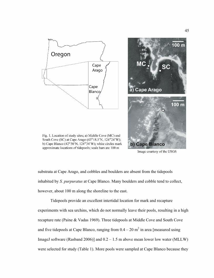
45
substrata at Cape Arago, and cobbles and boulders are absent from the tidepools
inhabited by S. purpuratus at Cape Blanco. Many boulders and cobble tend to collect,
however, about 100 m along the shoreline to the east.
Tidepools provide an excellent intertidal location for mark and recapture
experiments with sea urchins, which do not normally leave their pools, resulting in a high
recapture rate (Paine & Vadas 1969). Three tidepools at Middle Cove and South Cove
and five tidepools at Cape Blanco, ranging from 0.4 – 20 m2 in area [measured using
ImageJ software (Rasband 2006)] and 0.2 – 1.5 m above mean lower low water (MLLW)
were selected for study (Table 1). More pools were sampled at Cape Blanco because they

46
tended to be smaller in area with fewer purple sea urchins than those at the other sites.
Tidepools were selected haphazardly while keeping in mind the purposes of the growth
study. In order to produce accurate growth curves, it was necessary to use tidepools
containing a wide size range of S. purpuratus living inside and outside pits.
Strongylocentrotus purpuratus often situates itself to maximize the protection it
gains from its surroundings. If one is not completely protected in a deep pit, it might be
sitting in a shallow pit, squeezed into a crevice, tucked under a boulder, or even wedged
between other urchins. For this study, every sea urchins was categorized as either a “pit
urchins” or a “nonpit urchin.” An urchin was determined to be a pit urchin if its ambitus
(the equator, or widest point of the urchin) was level with or below the edge of a pit.
Some “nonpit urchins” were situated inside depressions that were shallow enough to be
considered nonpit microhabitats; such shallow depressions would not seem to constrain
growth or the ability to capture food in these nonpit urchins, compared to pit urchins that
are surrounded by rock.
Mark-Recapture Methods
Purple sea urchins were tagged with tetracycline during low tides in the
spring of 2005 (Kobayashi & Taki 1969, Ebert 1999a). Tetracycline, which fluoresces
under ultraviolet light, is bound along with calcite in the growing tests and lantern parts
of sea urchins. Sea urchins were removed from a tidepool and a hypodermic needle was
used to inject 0.2 mL of a solution containing 1 mg tetracycline per 10 mL seawater. The
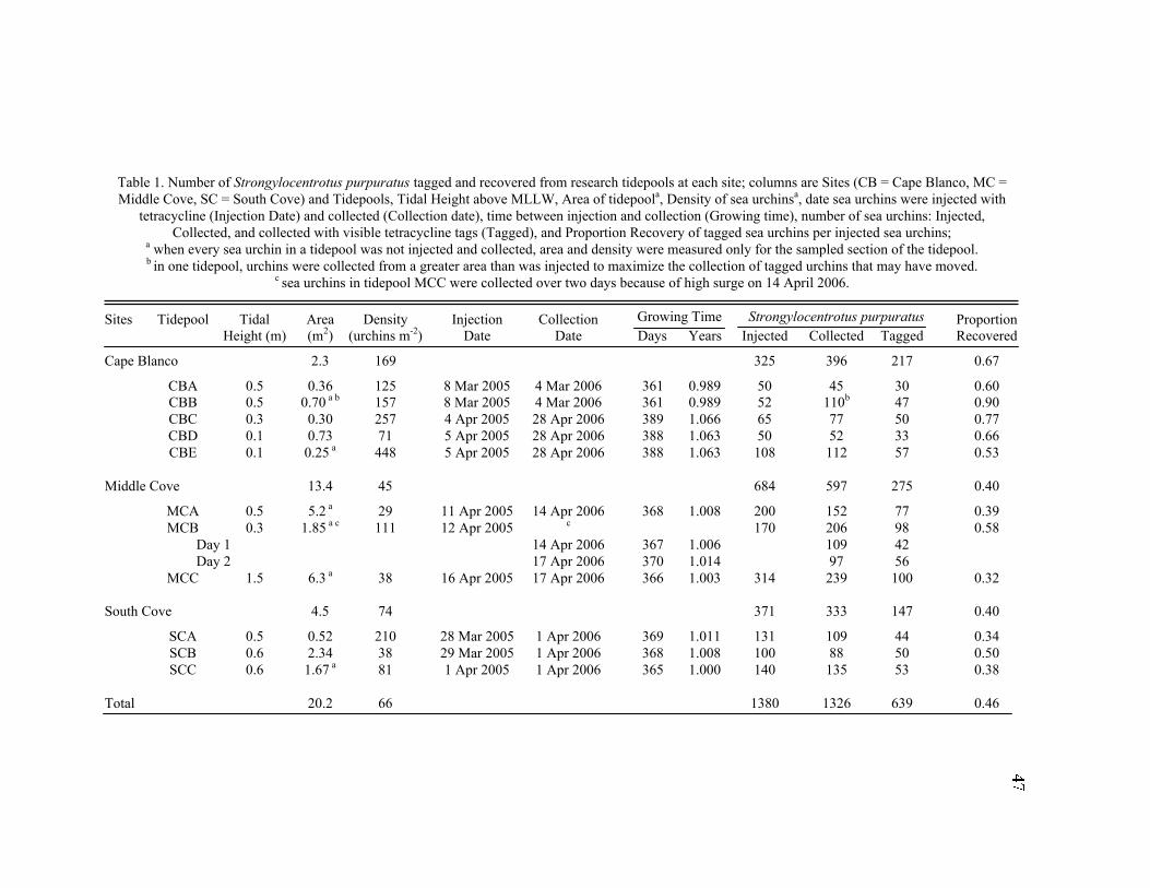
Table 1. Number of Strongylocentrotus purpuratus tagged and recovered from research tidepools at each site; columns are Sites (CB = Cape Blanco, MC =
Middle Cove, SC = South Cove) and Tidepools, Tidal Height above MLLW, Area of tidepoola, Density of sea urchins
a, date sea urchins were injected with
tetracycline (Injection Date) and collected (Collection date), time between injection and collection (Growing time), number of sea urchins: Injected,
Collected, and collected with visible tetracycline tags (Tagged), and Proportion Recovery of tagged sea urchins per injected sea urchins;a when every sea urchin in a tidepool was not injected and collected, area and density were measured only for the sampled section of the tidepool.
b in one tidepool, urchins were collected from a greater area than was injected to maximize the collection of tagged urchins that may have moved.
c sea urchins in tidepool MCC were collected over two days because of high surge on 14 April 2006.
Sites Tidepool Tidal Area Density Injection Collection Growing Time Strongylocentrotus purpuratus Proportion
Height (m) (m2) (urchins m
-2) Date Date Days Years Injected Collected Tagged Recovered
Cape Blanco 2.3 169 325 396 217 0.67
CBA 0.5 0.36 125 8 Mar 2005 4 Mar 2006 361 0.989 50 45 30 0.60
CBB 0.5 0.70 a b
157 8 Mar 2005 4 Mar 2006 361 0.989 52 110b
47 0.90
CBC 0.3 0.30 257 4 Apr 2005 28 Apr 2006 389 1.066 65 77 50 0.77
CBD 0.1 0.73 71 5 Apr 2005 28 Apr 2006 388 1.063 50 52 33 0.66
CBE 0.1 0.25 a
448 5 Apr 2005 28 Apr 2006 388 1.063 108 112 57 0.53
Middle Cove 13.4 45 684 597 275 0.40
MCA 0.5 5.2 a
29 11 Apr 2005 14 Apr 2006 368 1.008 200 152 77 0.39
MCB 0.3 1.85 a c
111 12 Apr 2005c
170 206 98 0.58
Day 1 14 Apr 2006 367 1.006 109 42
Day 2 17 Apr 2006 370 1.014 97 56
MCC 1.5 6.3 a
38 16 Apr 2005 17 Apr 2006 366 1.003 314 239 100 0.32
South Cove 4.5 74 371 333 147 0.40
SCA 0.5 0.52 210 28 Mar 2005 1 Apr 2006 369 1.011 131 109 44 0.34
SCB 0.6 2.34 38 29 Mar 2005 1 Apr 2006 368 1.008 100 88 50 0.50
SCC 0.6 1.67 a
81 1 Apr 2005 1 Apr 2006 365 1.000 140 135 53 0.38
Total 20.2 66 1380 1326 639 0.46
48
needle was inserted into the peristomial membrane covering the Aristotle’s lantern so that
the tetracycline solution would remain in the body cavity around the lantern. The sea
urchin was then replaced in the position from which it was taken. Visual observations
confirmed that sea urchins did not usually move when returned to the tidepool, though pit
urchins immediately retreated to the bottom of their pit. An effort was made to mark
every sea urchin in one or two tidepools during one low tide. When a tidepool was too
large or the sea urchins were too dense to mark every individual, all the sea urchins in
one distinct portion of the tidepool were tagged to increase the likelihood of recovery.
In the spring of 2006, one year after tagging, all of the purple sea urchins were
collected from the research tidepools. In the cases in which sea urchins in one section of
the tidepool were tagged, only animals in that section were collected. It is impossible to
tell by visual inspection if a sea urchin has been injected with tetracycline, but because
Strongylocentrotus purpuratus is largely sedentary in tidepools (see Chapter IV), most of
the collected animals had likely been marked. Sea urchins were sexed by removing the
peristomial membrane and checking for ripe gonads. They were then placed into
individually numbered containers and covered with 6.25% sodium hypochlorite (bleach)
to dissolve their soft tissue. After 24 hours, the tests and jaws were rinsed and left to soak
in hot water for one more day before being rinsed, air-dried, and stored in individually
labeled bags.
The test diameter, height, and demipyramid (jaw) length of each sea urchin were
measured with vernier calipers accurate to 0.001 cm, but repeated measures of an
individual could vary by as much as 0.1 cm. Jaw length and test diameter are highly

49
correlated in sea urchins (Ebert 1980b), so increments in jaw growth are generally
proportional to growth in test diameter. The length of the jaw is defined as the distance
between the oral tip (the labial end) and the shoulder at the esophageal end. Growth
occurs at both ends of a sea urchin jaw. The labial end is not worn away by scraping
because a tooth, held by two demipyramids, contacts food and rock. Jaws were
illuminated with ultraviolet light (Blak Ray longwave ultraviolet lamp) in a dark room
and inspected for glowing, yellow tetracycline marks. The length of the demipyramid
between the tag marks indicates size at the time of injection. Growth increments at the
labial and esophageal ends were recorded for each sea urchin using a dissecting
microscope (Leica Wild M37) and ocular micrometer with demarcations of 0.0026 cm.
The length of the jaw at the time of tagging was measured as the total jaw length minus
the two growth increments. All raw data are contained in Appendix C.
Growth in sites and microhabitats
A two-way analysis of covariance (ANCOVA) using the generalized linear model
(GLM) provided a statistical comparison of growth between sites and microhabitats for
purple sea urchins (Wilkinson 2004). The log transformation of (jaw growth + 0.01 cm)
was used as the response variable, because this transformation resulted in the best linear
relationship with the covariate jaw length (cm). Site and microhabitat were both fixed
factors. Data from South Cove were excluded from the ANCOVA to avoid violating the
assumption of homogeneous slopes (Fig. 2A). The regression line for South Cove showed
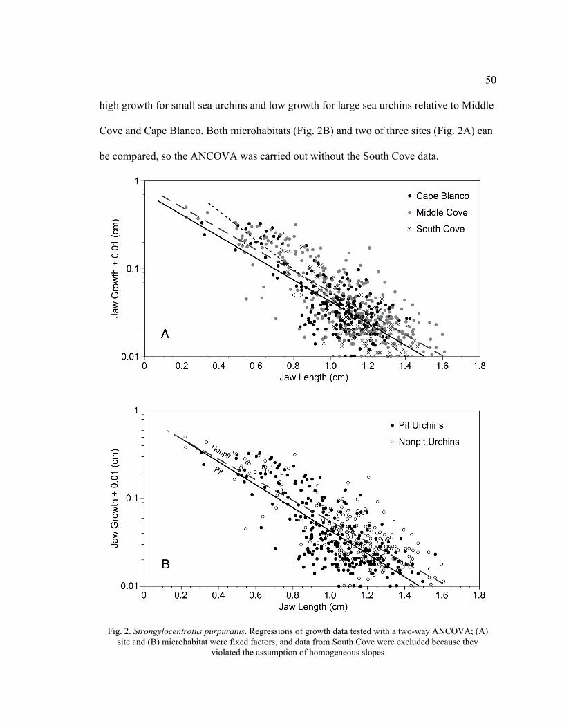
50
high growth for small sea urchins and low growth for large sea urchins relative to Middle
Cove and Cape Blanco. Both microhabitats (Fig. 2B) and two of three sites (Fig. 2A) can
be compared, so the ANCOVA was carried out without the South Cove data.
Fig. 2. Strongylocentrotus purpuratus. Regressions of growth data tested with a two-way ANCOVA; (A)
site and (B) microhabitat were fixed factors, and data from South Cove were excluded because they
violated the assumption of homogeneous slopes
51
Growth model
The Tanaka growth function
Growth in Strongylocentrotus purpuratus was modeled with the Tanaka function
(Tanaka 1982, 1988). This technique allows the comparison of instantaneous growth
rates between sea urchins in different microhabitats, sites, and tidepools. An
indiscriminate growth model, the Tanaka function models the growth of organisms
characterized by an early lag in growth, followed by a period of exponential growth that
soon declines, but never to zero. Ebert (1999b) clearly explained the theory and
application of the Tanaka growth function using S. franciscanus. Though this model was
not developed specifically for any organism, it has been applied mainly to echinoids,
including S. franciscanus (Ebert & Russell 1993, Ebert 1999a, Ebert & Southon 2003), S.
droebachiensis (Russell et al. 1998, Russell 2001), and Evechinus chloroticus (McShane
& Anderson 1997, Lamare & Mladenov 2000), as well as several other taxa, including
the ophiuroids Astrobrachion constrictum (Stewart & Mladenov 1997) and Ophiocten
hastatum (Gage et al. 2004) and the bivalve Nuttalia obscurata (Dudas 2005). Though
sea urchin growth has also been modeled with the Richards (Ebert 1980a, Russell 1987,
Kenner 1992), Bertalanffy (Ebert 1977, Barry & Tegner 1990, Morgan et al. 2000), and
other growth functions (Jordana et al. 1997, Grosjean et al. 2003), a visual examination
indicated that the Tanaka function provided the best fit to the growth data.
In the Tanaka function, the size of an organism at time t (St) is defined as:
�
St =1
fln2f(t - c) + 2 f
2(t - c)
2+ fa + d (1)
52
The four parameters do not all have clear biological meanings, but Tanaka (1988) defines
them as such:
a = a measure of the maximum growth rate, which is at
�
1
a,
c = age at which growth rate is maximum
d = a parameter that shifts the body size at which growth is maximum, and
f = a measure of the rate of change of the growth rate (Ebert 1999b)
The Tanaka function can be modified into a three-parameter “difference” equation so
that an organism’s resulting size after growth (St+1) can be calculated as:
�
St+1
=1
fln2G + 2 G
2+ fa + d (2)
where
�
G =E
4-fa
E+ f (3)
and
�
E = ef S
t-d( )( )
. (4)
By reducing the number of parameters that need to be estimated to three, the difference
equation improves the model’s ability to create a curve that tightly fits the data.
In the manner of Ebert (1999a), one parameter was varied at a time to get a better
sense of how each influences the overall growth curve (Fig. 3A), which is a measure of
instantaneous growth rate a given size. Growth curves generated by the Tanaka function
can be integrated to calculate overall size as a function of age (Fig. 3B). An increase in
the growth parameter f accelerates the growth curve’s climb to maximum size, but also
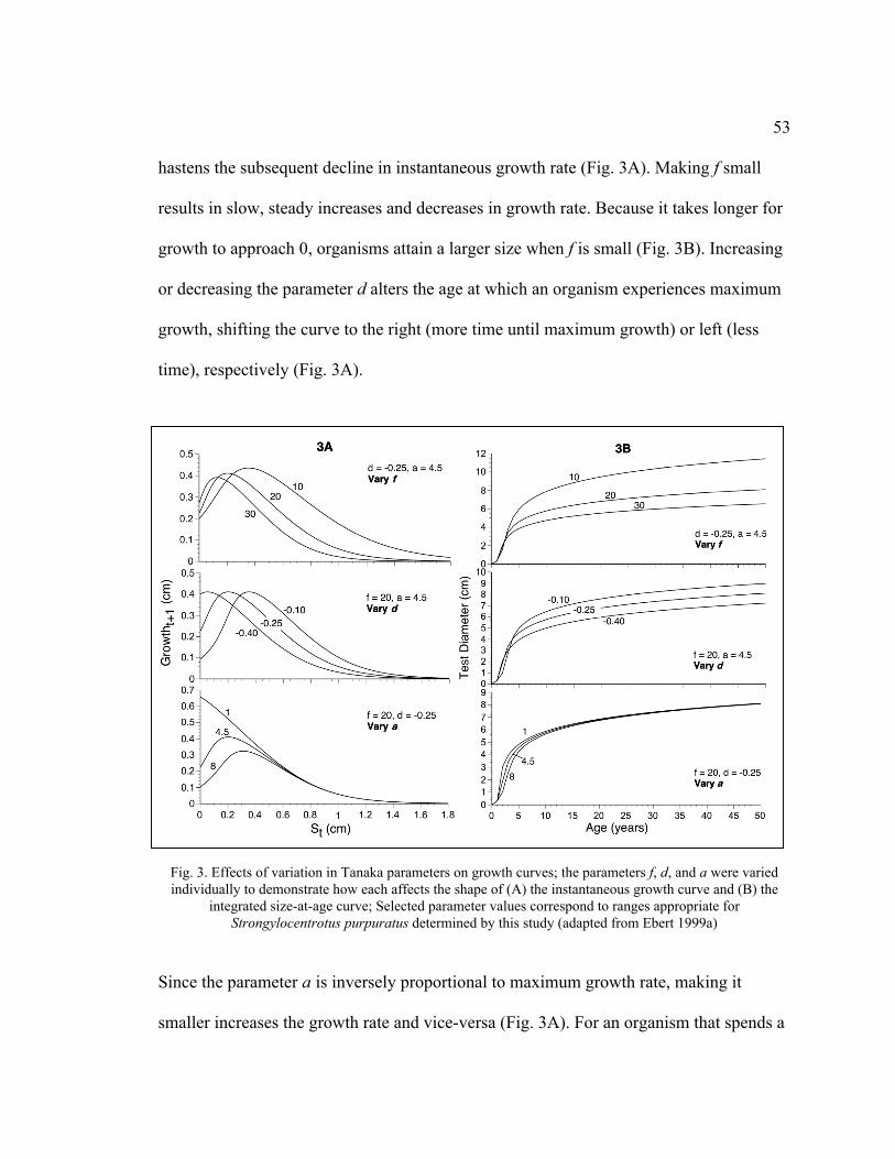
53
hastens the subsequent decline in instantaneous growth rate (Fig. 3A). Making f small
results in slow, steady increases and decreases in growth rate. Because it takes longer for
growth to approach 0, organisms attain a larger size when f is small (Fig. 3B). Increasing
or decreasing the parameter d alters the age at which an organism experiences maximum
growth, shifting the curve to the right (more time until maximum growth) or left (less
time), respectively (Fig. 3A).
Fig. 3. Effects of variation in Tanaka parameters on growth curves; the parameters f, d, and a were varied
individually to demonstrate how each affects the shape of (A) the instantaneous growth curve and (B) the
integrated size-at-age curve; Selected parameter values correspond to ranges appropriate for
Strongylocentrotus purpuratus determined by this study (adapted from Ebert 1999a)
Since the parameter a is inversely proportional to maximum growth rate, making it
smaller increases the growth rate and vice-versa (Fig. 3A). For an organism that spends a
54
very small proportion of its life in this phase of rapid growth, such as Strongylocentrotus
purpuratus, changing a impacts the overall size less than changing the parameters d and
especially f (Fig. 3B).
Applying the Tanaka function to the growth data
Jaw size at the time of tetracycline tagging (Jt) and final jaw size (Jt+1) were used
in nonlinear regressions (Systat Software, Wilkinson 2004) to calculate the Tanaka
parameters f, d, and a, describing the growth of Strongylocentrotus purpuratus from
different microhabitats and sites. Growth was also compared between tidepools at Middle
Cove, the only site with enough tagged sea urchins within individual tidepools that
Tanaka growth curves could be created for each. Instantaneous growth curves (Jt+1 – Jt
plotted as a function of Jt) were generated by inserting the calculated parameters back
into the Tanaka model (Eq. 2 – 4).
In nonlinear regression, parameter estimation can be problematic when growth
data for some size classes, especially small ones, are missing (Kenner 1992). Small
urchins accounted for such a small proportion of the data in some groups that nonlinear
regression resulted either in an improper Tanaka curve or the inability to fit any curve to
the data. To deal with the general rarity of small Strongylocentrotus purpuratus, all
individuals from all tidepools with an initial jaw size <0.75 cm (approximately two year-
old urchins and younger with test diameters <3.2 cm) were pooled into a single group of
55
sea urchins designated as “young”. These pooled young urchins were used to calculate
every nonlinear regression.
Bootstrap methods were applied to the nonlinear regressions to estimate means
and confidence intervals of the Tanaka parameters (McPeek & Kalisz 1993). One
thousand bootstraps were performed and the bootstrapped parameter estimates (BPE)
were obtained by accounting for bias. After sorting the bootstraps from smallest to
largest, 95% confidence intervals were calculated as the average of the 25th
and 26th
samples, and the average of the 975th
and 976th
samples (Dixon 1993). Differences in
Tanaka parameters between treatments were detected by examining the BPEs and
confidence intervals.
Age estimation
The difference equation (Eq. 2-4) can be used to create size-at-age curves for each
set of Tanaka parameters if size is known for the first-year age group. In this case, Jt was
estimated to be 0.1 cm, which is the smallest jaw that was measured in any sea urchin and
is the approximate jaw size for a one-year old purple sea urchin (Kenner 1992). Eq. 2
gives Jt+1, which is the jaw size at year 1. Jt+1 is then reentered into Eq. 4 as Jt and so on,
until a range of ages and corresponding sizes can be plotted. This method of integrating
the Tanaka function over time was used to create size-at-age curves for each set of
Tanaka parameters. A power curve was used to describe the allometric relationship
between jaw size and test diameter so that test diameter could also be expressed as a
56
function of age. Age was calculated for the jaws of all collected Strongylocentrotus
purpuratus (tagged and untagged), and age-frequency distributions were created for sites,
microhabitats, and Middle Cove tidepools.
RESULTS
Growth in sites and microhabitats
The growth of Strongylocentrotus purpuratus living in pit and nonpit
microhabitats can be compared in three ways: 1) ANCOVA of the log transformation of
growth rate; 2) visual examination of nonlinear regressions fit to the Tanaka function; 3)
comparison of the associated Tanaka parameters and confidence intervals. All three
techniques demonstrate that S. purpuratus grew faster outside of pits than inside pits.
Differences in growth rate between sites and microhabitats were tested with a two-way
fixed factor ANCOVA on the log-transformed growth increments. The results of the
ANCOVA and adjusted least square means are presented in Table 2. The nonsignificant
interaction (P > 0.25) was removed and its variance was pooled with the residual
(Underwood 1997). The growth data from South Cove violated the homogeneous slopes
assumption because large sea urchins from that site had very small growth increments
(Fig. 2A); these data were excluded from the analysis allowing only a comparison
between Cape Blanco and Middle Cove. Jaw growth varied significantly by site and
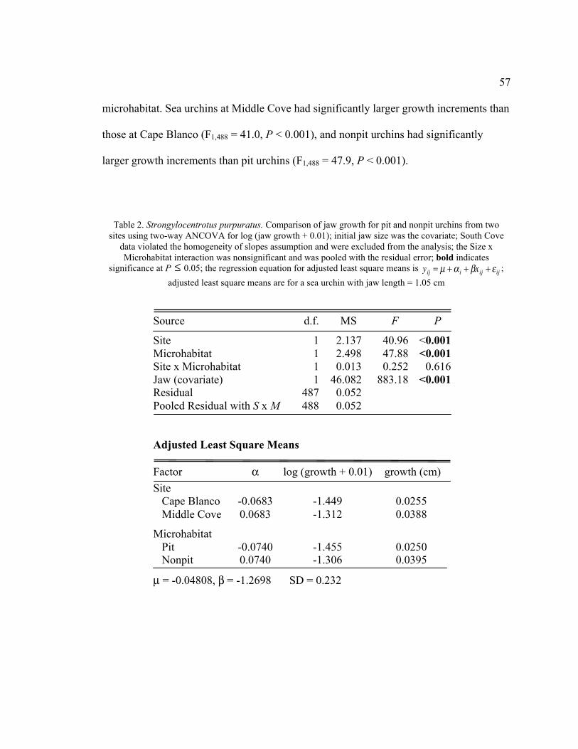
57
microhabitat. Sea urchins at Middle Cove had significantly larger growth increments than
those at Cape Blanco (F1,488 = 41.0, P < 0.001), and nonpit urchins had significantly
larger growth increments than pit urchins (F1,488 = 47.9, P < 0.001).
Table 2. Strongylocentrotus purpuratus. Comparison of jaw growth for pit and nonpit urchins from two
sites using two-way ANCOVA for log (jaw growth + 0.01); initial jaw size was the covariate; South Cove
data violated the homogeneity of slopes assumption and were excluded from the analysis; the Size x
Microhabitat interaction was nonsignificant and was pooled with the residual error; bold indicates
significance at P
�
£ 0.05; the regression equation for adjusted least square means is
�
yij = m + a i + bxij + e ij ;
adjusted least square means are for a sea urchin with jaw length = 1.05 cm
Source d.f. MS F P
Site 1 2.137 40.96 <0.001
Microhabitat 1 2.498 47.88 <0.001
Site x Microhabitat 1 0.013 0.252 0.616
Jaw (covariate) 1 46.082 883.18 <0.001
Residual 487 0.052
Pooled Residual with S x M 488 0.052
Adjusted Least Square Means
Factor a log (growth + 0.01) growth (cm)
Site
Cape Blanco -0.0683 -1.449 0.0255
Middle Cove 0.0683 -1.312 0.0388
Microhabitat
Pit -0.0740 -1.455 0.0250
Nonpit 0.0740 -1.306 0.0395
m = -0.04808, b = -1.2698 SD = 0.232
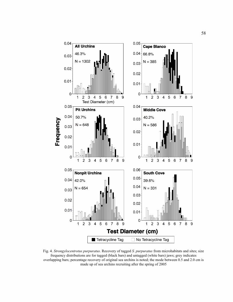
58
Fig. 4. Strongylocentrotus purpuratus. Recovery of tagged S. purpuratus from microhabitats and sites; size
frequency distributions are for tagged (black bars) and untagged (white bars) jaws; grey indicates
overlapping bars; percentage recovery of original sea urchins is noted; the mode between 0.5 and 2.0 cm is
made up of sea urchins recruiting after the spring of 2005
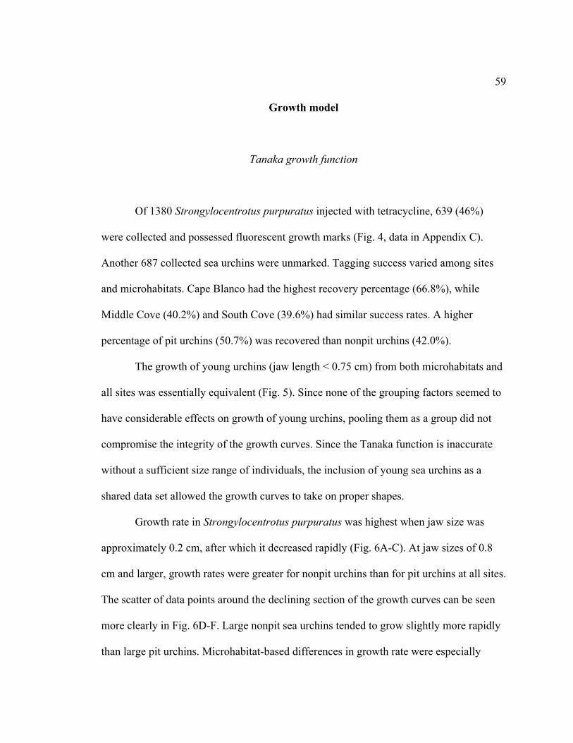
59
Growth model
Tanaka growth function
Of 1380 Strongylocentrotus purpuratus injected with tetracycline, 639 (46%)
were collected and possessed fluorescent growth marks (Fig. 4, data in Appendix C).
Another 687 collected sea urchins were unmarked. Tagging success varied among sites
and microhabitats. Cape Blanco had the highest recovery percentage (66.8%), while
Middle Cove (40.2%) and South Cove (39.6%) had similar success rates. A higher
percentage of pit urchins (50.7%) was recovered than nonpit urchins (42.0%).
The growth of young urchins (jaw length < 0.75 cm) from both microhabitats and
all sites was essentially equivalent (Fig. 5). Since none of the grouping factors seemed to
have considerable effects on growth of young urchins, pooling them as a group did not
compromise the integrity of the growth curves. Since the Tanaka function is inaccurate
without a sufficient size range of individuals, the inclusion of young sea urchins as a
shared data set allowed the growth curves to take on proper shapes.
Growth rate in Strongylocentrotus purpuratus was highest when jaw size was
approximately 0.2 cm, after which it decreased rapidly (Fig. 6A-C). At jaw sizes of 0.8
cm and larger, growth rates were greater for nonpit urchins than for pit urchins at all sites.
The scatter of data points around the declining section of the growth curves can be seen
more clearly in Fig. 6D-F. Large nonpit sea urchins tended to grow slightly more rapidly
than large pit urchins. Microhabitat-based differences in growth rate were especially
60
Fig. 5. Strongylocentrotus purpuratus. Growth increments over one year as a function of initial jaw length
(Jt) for young S. purpuratus (Jt < 0.75 cm; approximate test diameter < 3.2 cm); sites are denoted by
symbol shape, pit urchins are dark symbols, as nonpit urchins are light symbols
apparent at Middle Cove and Cape Blanco, while differences in growth rate were less
clear at South Cove.
It should be noted that this analysis was unable to speak toward differences in the
growth rates of small sea urchins from different microhabitats or sites. Since the pooled
young urchins were included in each nonlinear regression, the early sections of the
growth curves are similar. Differences between curves are driven solely by the effects of
larger sea urchins and the necessary initial growth lag and sigmoidal shape of the Tanaka
function.

61
Fig. 6. Strongylocentrotus purpuratus. Tanaka function fit to jaw growth data for pit urchins (open circles)
and nonpit urchins (filled circles) at three sites; the Tanaka curves are solid for pit urchins and dashed for
nonpit urchins; data for young S. purpuratus with jaw length <0.75 cm were pooled (x); jaw growth
increments are for one year of field growth, and initial jaw length (Jt) is the independent variable; (A–C)
instantaneous growth rates for all sizes of S. purpuratus, and the dashed line marks the vertical axis for
(D–F) where jaw length >0.80 cm
62
Tanaka function parameters
For the entire data set and individual sites, the Tanaka parameters f and d are both
smaller in regressions fitted to nonpit urchins than to pit urchins (Fig. 7). The
bootstrapped 95% confidence intervals of these parameters overlap slightly between
microhabitats at Middle Cove, a bit more at Cape Blanco, and extensively at South Cove,
indicating that microhabitat’s effect on growth was dependent on the site. Of the three
parameters, f varied the most between microhabitats, as its confidence intervals
overlapped less than those of d or a for each site and overall. Recall that f is a measure of
the rate of change in growth; nonpit urchins, with lower f values than pit urchins,
experienced a slower decrease in growth rate, which is demonstrated by the growth
curves in Fig. 6A–C. This slower deceleration in growth means that nonpit urchins
maintained higher growth rates than pit urchins in all sizes larger than the pooled young
urchins.
The effects of pooling the young urchins can be seen in Fig. 7, which reports and
displays the Tanaka parameters and confidence intervals for different microhabitats at
each site. The parameter a did not vary much between groups, and its confidence
intervals were almost completely overlapping. When data for all sea urchins are pooled, a
is 4.62, which corresponds to an approximate maximum growth rate of 0.465 cm year-1
(
�
a-1
). This maximum growth occurred when sea urchins were less than one year old,
and jaw length was about 0.2 cm. While this growth rate is likely an accurate measure for
the population, the pooling technique prevents drawing conclusions for any group factors.
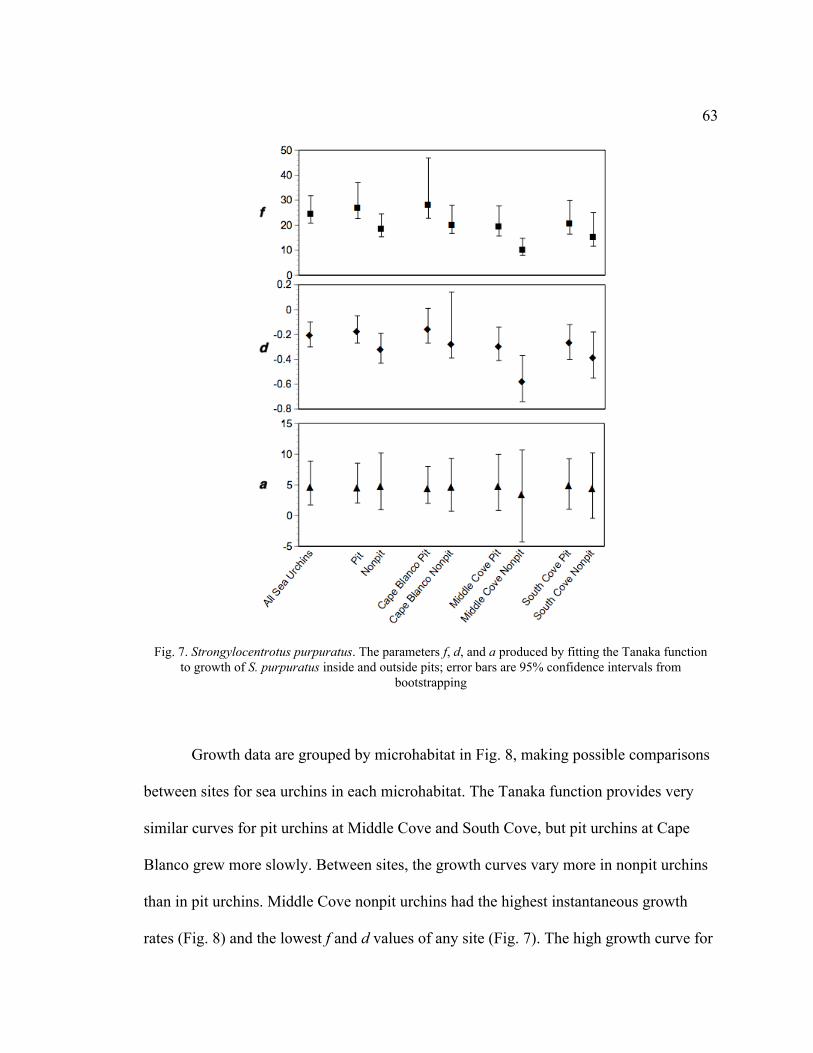
63
Fig. 7. Strongylocentrotus purpuratus. The parameters f, d, and a produced by fitting the Tanaka function
to growth of S. purpuratus inside and outside pits; error bars are 95% confidence intervals from
bootstrapping
Growth data are grouped by microhabitat in Fig. 8, making possible comparisons
between sites for sea urchins in each microhabitat. The Tanaka function provides very
similar curves for pit urchins at Middle Cove and South Cove, but pit urchins at Cape
Blanco grew more slowly. Between sites, the growth curves vary more in nonpit urchins
than in pit urchins. Middle Cove nonpit urchins had the highest instantaneous growth
rates (Fig. 8) and the lowest f and d values of any site (Fig. 7). The high growth curve for
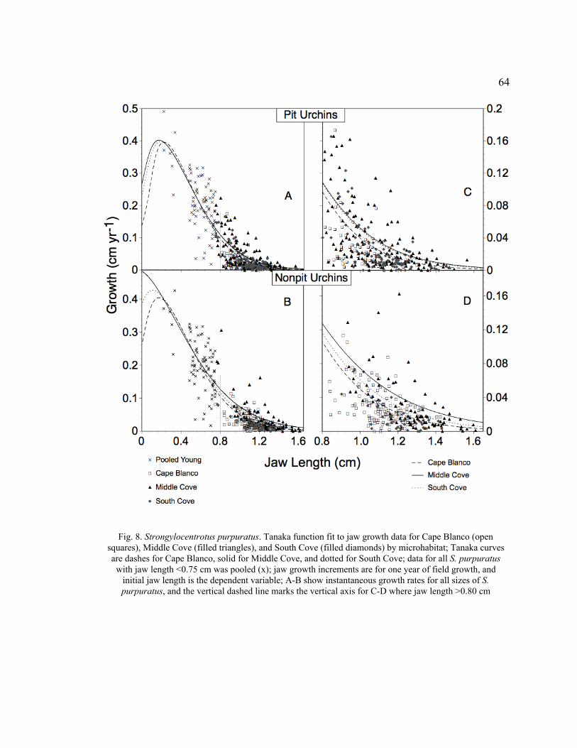
64
Fig. 8. Strongylocentrotus purpuratus. Tanaka function fit to jaw growth data for Cape Blanco (open
squares), Middle Cove (filled triangles), and South Cove (filled diamonds) by microhabitat; Tanaka curves
are dashes for Cape Blanco, solid for Middle Cove, and dotted for South Cove; data for all S. purpuratus
with jaw length <0.75 cm was pooled (x); jaw growth increments are for one year of field growth, and
initial jaw length is the dependent variable; A-B show instantaneous growth rates for all sizes of S.
purpuratus, and the vertical dashed line marks the vertical axis for C-D where jaw length >0.80 cm
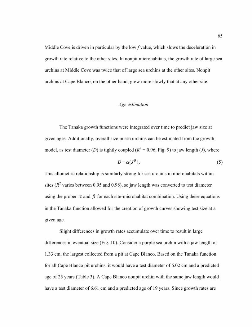
65
Middle Cove is driven in particular by the low f value, which slows the deceleration in
growth rate relative to the other sites. In nonpit microhabitats, the growth rate of large sea
urchins at Middle Cove was twice that of large sea urchins at the other sites. Nonpit
urchins at Cape Blanco, on the other hand, grew more slowly that at any other site.
Age estimation
The Tanaka growth functions were integrated over time to predict jaw size at
given ages. Additionally, overall size in sea urchins can be estimated from the growth
model, as test diameter (D) is tightly coupled (R2 = 0.96, Fig. 9) to jaw length (J), where
�
D = a(Jb). (5)
This allometric relationship is similarly strong for sea urchins in microhabitats within
sites (R2 varies between 0.95 and 0.98), so jaw length was converted to test diameter
using the proper
�
a and
�
b for each site-microhabitat combination. Using these equations
in the Tanaka function allowed for the creation of growth curves showing test size at a
given age.
Slight differences in growth rates accumulate over time to result in large
differences in eventual size (Fig. 10). Consider a purple sea urchin with a jaw length of
1.33 cm, the largest collected from a pit at Cape Blanco. Based on the Tanaka function
for all Cape Blanco pit urchins, it would have a test diameter of 6.02 cm and a predicted
age of 25 years (Table 3). A Cape Blanco nonpit urchin with the same jaw length would
have a test diameter of 6.61 cm and a predicted age of 19 years. Since growth rates are
66
Fig. 9. Strongylocentrotus purpuratus. Power relationship between jaw length and test diameter in pit and
nonpit urchins; high R2 values allow size to be expressed in terms of test diameter in Fig. 10, 13, and 15
higher at Middle Cove, a pit urchin with the same jaw length is predicted to be 18 years
old with a test diameter of 6.37 cm, while a nonpit urchin might be just 11 years old with
a test diameter of 6.75 cm. At each site, this pattern becomes more pronounced with older
sea urchins. At the age of 30, nonpit urchins have test diameters approximately 1 cm
greater than do pit urchins at all sites, and the difference is 1.5 cm at Middle Cove. The
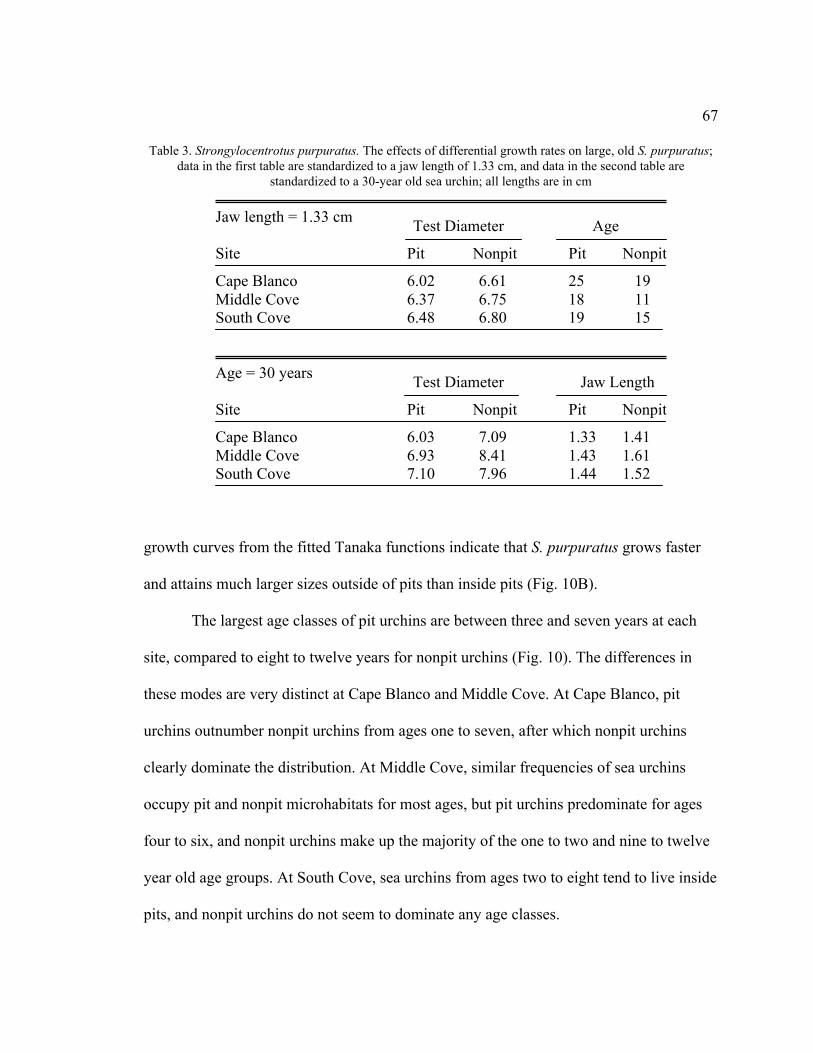
67
Table 3. Strongylocentrotus purpuratus. The effects of differential growth rates on large, old S. purpuratus;
data in the first table are standardized to a jaw length of 1.33 cm, and data in the second table are
standardized to a 30-year old sea urchin; all lengths are in cm
Jaw length = 1.33 cmTest Diameter Age
Site Pit Nonpit Pit Nonpit
Cape Blanco 6.02 6.61 25 19
Middle Cove 6.37 6.75 18 11
South Cove 6.48 6.80 19 15
Age = 30 yearsTest Diameter Jaw Length
Site Pit Nonpit Pit Nonpit
Cape Blanco 6.03 7.09 1.33 1.41
Middle Cove 6.93 8.41 1.43 1.61
South Cove 7.10 7.96 1.44 1.52
growth curves from the fitted Tanaka functions indicate that S. purpuratus grows faster
and attains much larger sizes outside of pits than inside pits (Fig. 10B).
The largest age classes of pit urchins are between three and seven years at each
site, compared to eight to twelve years for nonpit urchins (Fig. 10). The differences in
these modes are very distinct at Cape Blanco and Middle Cove. At Cape Blanco, pit
urchins outnumber nonpit urchins from ages one to seven, after which nonpit urchins
clearly dominate the distribution. At Middle Cove, similar frequencies of sea urchins
occupy pit and nonpit microhabitats for most ages, but pit urchins predominate for ages
four to six, and nonpit urchins make up the majority of the one to two and nine to twelve
year old age groups. At South Cove, sea urchins from ages two to eight tend to live inside
pits, and nonpit urchins do not seem to dominate any age classes.
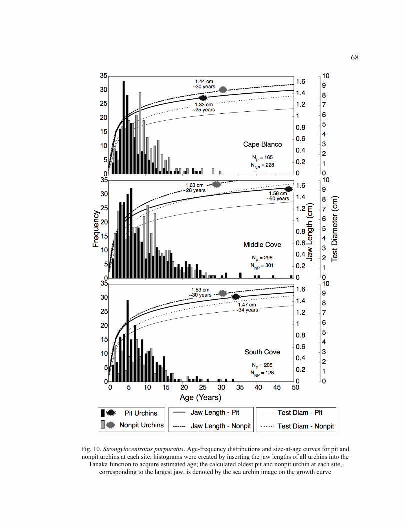
68
Fig. 10. Strongylocentrotus purpuratus. Age-frequency distributions and size-at-age curves for pit and
nonpit urchins at each site; histograms were created by inserting the jaw lengths of all urchins into the
Tanaka function to acquire estimated age; the calculated oldest pit and nonpit urchin at each site,
corresponding to the largest jaw, is denoted by the sea urchin image on the growth curve

69
Growth differences between sites and tidepools
Site differences were apparent when microhabitat was ignored and nonlinear
regression was used to fit the Tanaka function to the data from each site. Consistent with
the ANCOVA results, the fastest growth occurred at Middle Cove and the slowest at
Cape Blanco (Fig. 11). The Tanaka growth parameters and bootstrapped 95% confidence
intervals for data pooled by site and tidepool are presented in Fig. 12. The age-frequency
distributions, created from inserting jaw lengths into the growth curves integrated over
time (Fig. 13), show several modal age groups of Strongylocentrotus purpuratus. At
Cape Blanco, these modes occur at 4, 10, and 17 years, suggesting high recruitment
pulses in 2002, 1996, and 1989. Middle Cove has similar modes at 3 – 5, 12 – 13, and 17
years, suggesting especially successful recruitment in 2001 – 3, 1993 – 4, and 1989. The
distribution at South Cove is less clear, although there appear to be modes at 5- and 12-
years as in Middle Cove. Each population of S. purpuratus is long-lived, with the oldest
individuals close to 50 years old (Fig. 13).
Middle Cove was the only site with enough data to construct growth curves for
individual tidepools. Sea urchins in tidepool MCC grew much faster than those in MCA
or MCB (Fig. 14). This discrepancy in growth rates is reflected in extremely low values
for the Tanaka parameters f and d for MCC (Fig. 12). The 95% confidence intervals for f
and d do not overlap, suggesting that the growth of sea urchins in MCC was significantly
higher than in the other pools. Enough Strongylocentrotus purpuratus were collected
from MCC that the growth of pit and nonpit urchins could be evaluated separately in this
one tidepool. Differences between the Tanaka parameters were small, indicating very
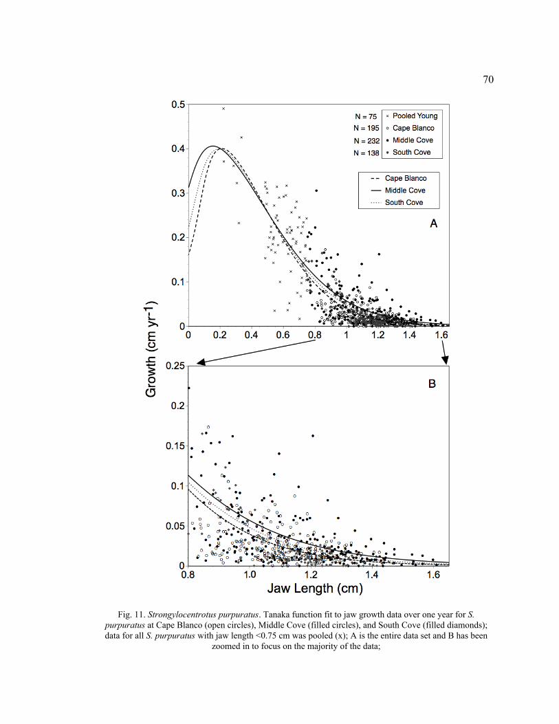
70
Fig. 11. Strongylocentrotus purpuratus. Tanaka function fit to jaw growth data over one year for S.
purpuratus at Cape Blanco (open circles), Middle Cove (filled circles), and South Cove (filled diamonds);
data for all S. purpuratus with jaw length <0.75 cm was pooled (x); A is the entire data set and B has been
zoomed in to focus on the majority of the data;
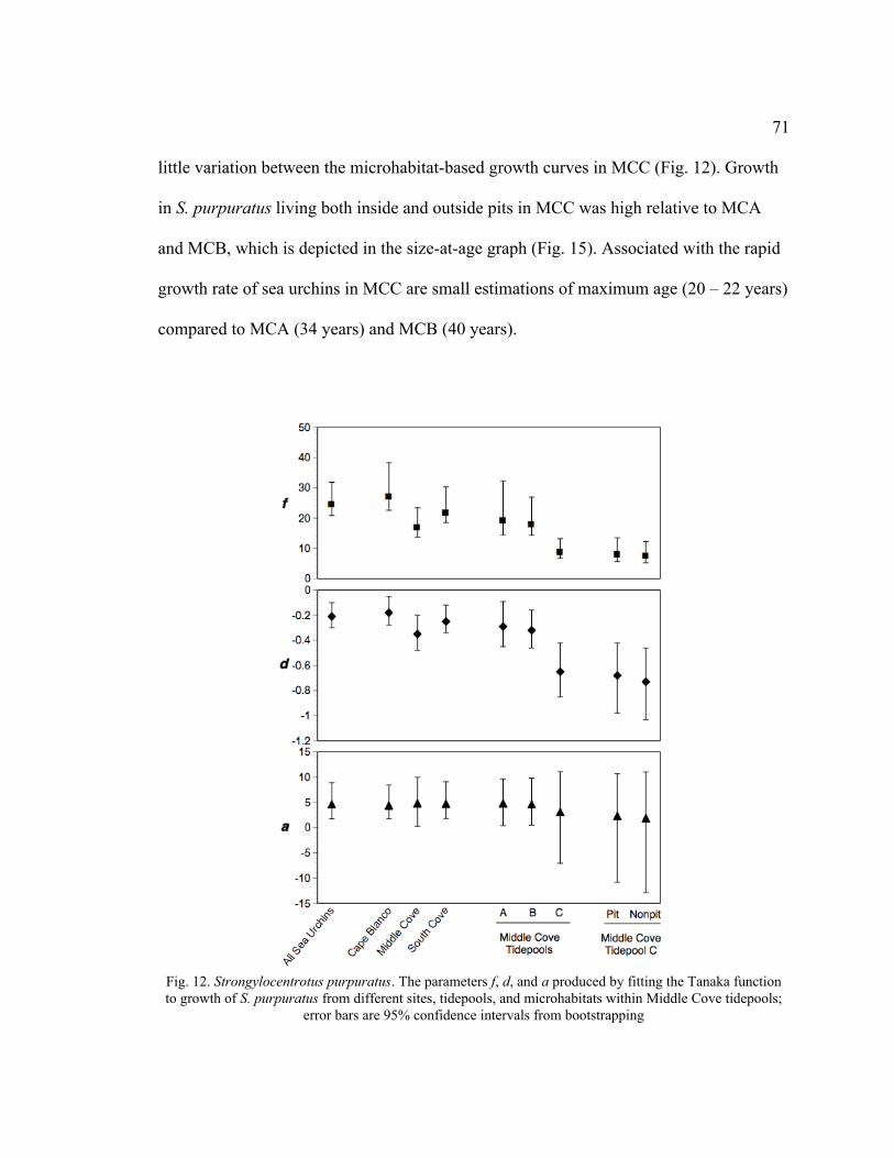
71
little variation between the microhabitat-based growth curves in MCC (Fig. 12). Growth
in S. purpuratus living both inside and outside pits in MCC was high relative to MCA
and MCB, which is depicted in the size-at-age graph (Fig. 15). Associated with the rapid
growth rate of sea urchins in MCC are small estimations of maximum age (20 – 22 years)
compared to MCA (34 years) and MCB (40 years).
Fig. 12. Strongylocentrotus purpuratus. The parameters f, d, and a produced by fitting the Tanaka function
to growth of S. purpuratus from different sites, tidepools, and microhabitats within Middle Cove tidepools;
error bars are 95% confidence intervals from bootstrapping
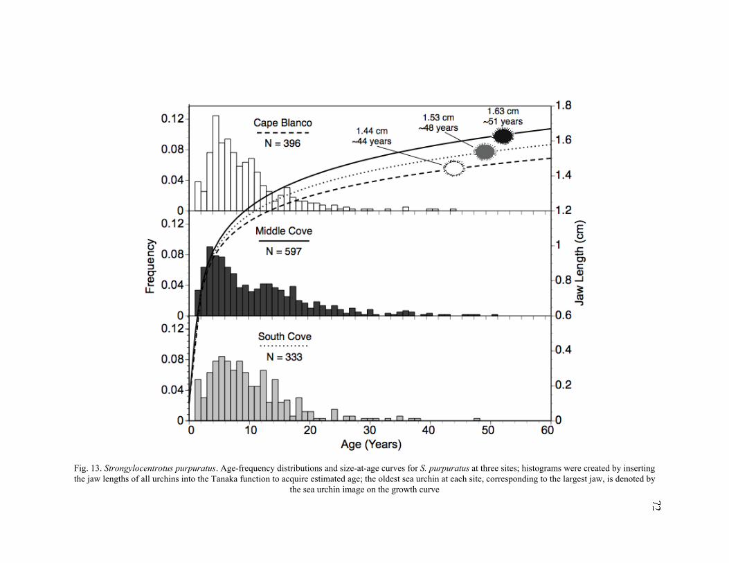
Fig. 13. Strongylocentrotus purpuratus. Age-frequency distributions and size-at-age curves for S. purpuratus at three sites; histograms were created by inserting
the jaw lengths of all urchins into the Tanaka function to acquire estimated age; the oldest sea urchin at each site, corresponding to the largest jaw, is denoted by
the sea urchin image on the growth curve

73
Visual inspection of Fig. 15 indicates that the age-frequency distributions in the
tidepools are different. MCA had high frequencies of S. purpuratus younger than five
years. MCB contained few sea urchins of these small size classes, and the modal age
appears to have been about 14 years. The data from MCC repeat the patterns seen at the
site level; the modal age of pit urchins is four to six years, and beyond eight years, nonpit
urchins were more numerous than pit urchins.
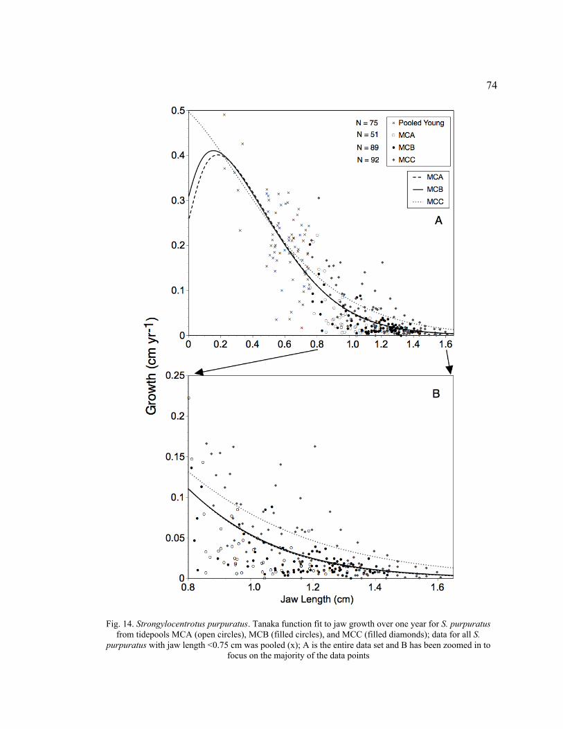
74
Fig. 14. Strongylocentrotus purpuratus. Tanaka function fit to jaw growth over one year for S. purpuratus
from tidepools MCA (open circles), MCB (filled circles), and MCC (filled diamonds); data for all S.
purpuratus with jaw length <0.75 cm was pooled (x); A is the entire data set and B has been zoomed in to
focus on the majority of the data points
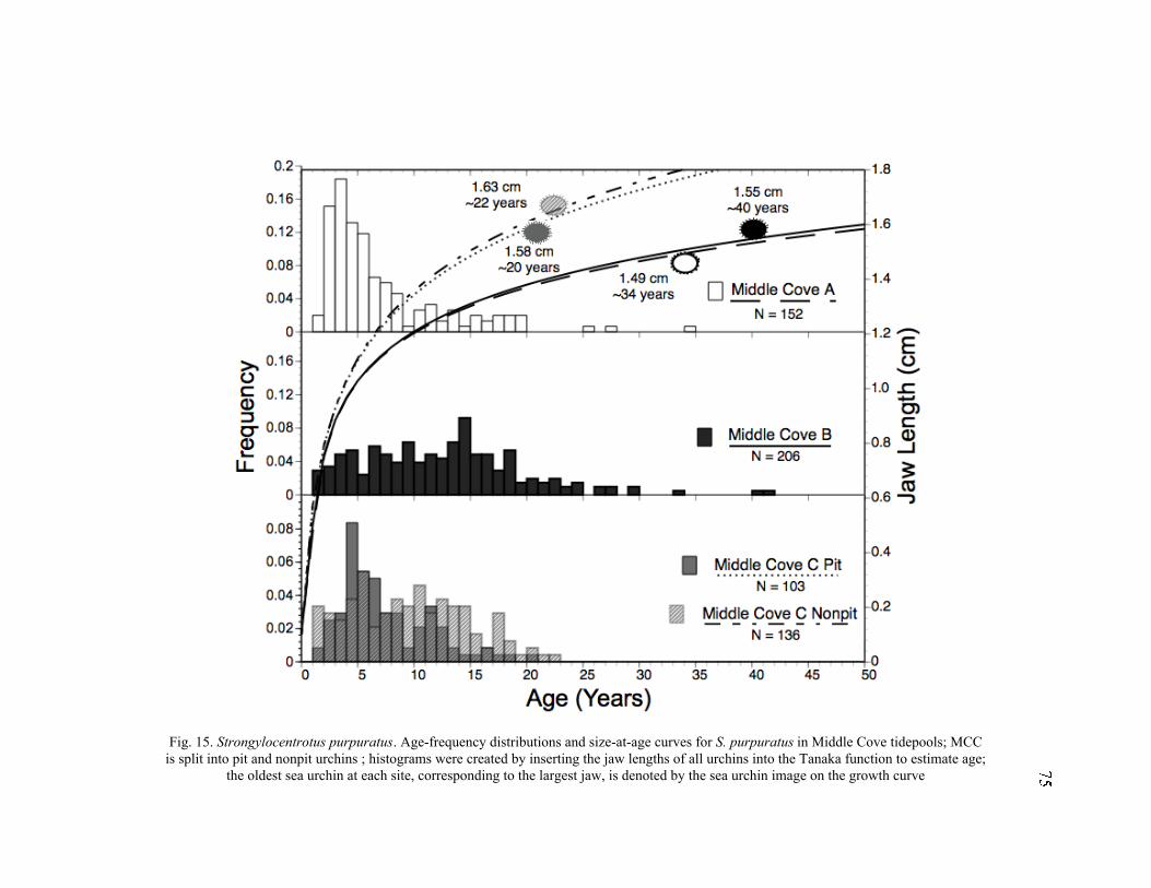
Fig. 15. Strongylocentrotus purpuratus. Age-frequency distributions and size-at-age curves for S. purpuratus in Middle Cove tidepools; MCC
is split into pit and nonpit urchins ; histograms were created by inserting the jaw lengths of all urchins into the Tanaka function to estimate age;
the oldest sea urchin at each site, corresponding to the largest jaw, is denoted by the sea urchin image on the growth curve

76
DISCUSSION
Lack of small sea urchins
All of the spatial scales investigated, microhabitats, tidepools, and sites, had
substantial effects on the growth of Strongylocentrotus purpuratus, despite several
shortcomings in the data. First, the nonlinear regressions were complicated by an
unavoidable lack of data in first-year S. purpuratus. No tetracycline-tagged sea urchin
had a test diameter <3 cm, corresponding to a two- or three-year old individual.
Inspection of the size-frequency distributions in Fig. 4 indicates that the first-year size
class was made up of untagged sea urchins with a test diameter less than 2 cm; in the
spring of 2005, these individuals were either cryptically hidden or had not yet recruited to
the tidepools. Thus, the data set did not include any sea urchins less than one-year old.
Yamaguchi (1975) pointed out that this lack of data in the youngest size classes limits the
ability of many studies to properly model growth in benthic invertebrates, which was true
in this case. In Fig. 16A, the Tanaka function has been applied to the data from Cape
Blanco without the pooled young urchins. The resulting exaggerated lag in growth of
juvenile S. purpuratus displays maximum growth to occur when jaw size is 0.4 – 0.5 cm;
at these growth rates, the size of maximum growth would not be reached until six to eight
years, which is a severe underestimation based on other studies (Ebert 1968, Rowley
1990, Kenner 1992). The best solution for this data set was to pool all juveniles with
initial jaw length less than 0.75 cm into a single group of data. My intention was to
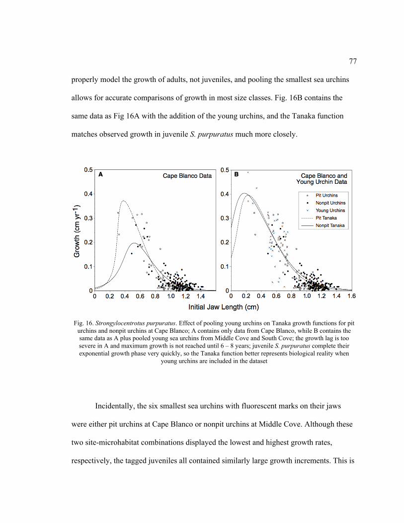
77
properly model the growth of adults, not juveniles, and pooling the smallest sea urchins
allows for accurate comparisons of growth in most size classes. Fig. 16B contains the
same data as Fig 16A with the addition of the young urchins, and the Tanaka function
matches observed growth in juvenile S. purpuratus much more closely.
Fig. 16. Strongylocentrotus purpuratus. Effect of pooling young urchins on Tanaka growth functions for pit
urchins and nonpit urchins at Cape Blanco; A contains only data from Cape Blanco, while B contains the
same data as A plus pooled young sea urchins from Middle Cove and South Cove; the growth lag is too
severe in A and maximum growth is not reached until 6 – 8 years; juvenile S. purpuratus complete their
exponential growth phase very quickly, so the Tanaka function better represents biological reality when
young urchins are included in the dataset
Incidentally, the six smallest sea urchins with fluorescent marks on their jaws
were either pit urchins at Cape Blanco or nonpit urchins at Middle Cove. Although these
two site-microhabitat combinations displayed the lowest and highest growth rates,
respectively, the tagged juveniles all contained similarly large growth increments. This is
78
too small a sample size from which to generalize, but the lack of distinct patterns in the
growth of small, tagged sea urchins increases the legitimacy of the pooling-the-young
technique. The diet of sea urchins changes as they age, so adults and juveniles could be
subjected to varying levels of food availability in the same tidepool (Breen et al. 1985,
Rowley 1990, Nishizaki & Ackerman 2004).
In most nonlinear regressions, plotting instantaneous growth rate against size
resulted in predicted maximum growth at a jaw length of 0.2 cm, equivalent to a juvenile
sea urchin less than one year old. The temporal resolution of this study is one year, and
upon recovery, no tagged sea urchin was determined to be younger than two years, so at
least the entire first year of growth is missing from the data. To increase the accuracy of
the Tanaka curve, the growth of juvenile S. purpuratus needs to be investigated in detail
over much shorter time intervals. Such small urchins cannot survive the puncture of their
peristomial membrane. Tagging post-settlement size classes usually involves
submergence in a calcein solution, which is incorporated into the skeleton and fluoresces
just like tetracycline (Russell & Urbaniak 2004).
Low recapture rate of tagged sea urchins
Given 1380 sea urchins were injected with tetracycline, the recapture of just 639
tagged animals seems low at first. This recapture rate of 46%, however, compares well
with success rates in other studies (Rowley 1990, McShane & Anderson 1997, Russell
2001). In the laboratory, tagging success is usually 100%, so why are field percentages

79
lower? Either the tetracycline did not tag all sea urchins, or some individuals moved or
died during the course of one year, so that half of the collected sea urchins had not been
tagged. The more probable explanation is that tetracycline was not bound into the jaws of
every sea urchin that was administered an injection. When viewed under ultraviolet light,
not all tagged jaws fluoresce equally. The brightest growth marks are seen on small jaws,
while large jaws from old individuals often possess very faint, almost undetectable
growth marks. This is because the faster a sea urchin grows, the more calcite – and
therefore, tetracycline – bound in its skeletal elements. Animals that are growing slowly
tend to incorporate less tetracycline, and if they not growing at all they will show no
growth mark. In this study, marking took place in the early spring when the intertidal was
relatively devoid of fleshy macroalgae, and many sea urchins likely had empty stomachs
and were not growing. Although the timing of injections resulted in the capture of the
entire growing season (summer and fall), delaying until later in the spring or summer
when macroalgal biomass is greater might have increased the tagging success.
If food limitation reduces tetracycline incorporation in the jaw, how can the
relatively high recapture rate at Cape Blanco be explained in light of the food limitation
in that population (see Chapter II)? One reasonable explanation is that sea urchins at
Cape Blanco incorporated more tetracycline simply because they were growing faster at
that particular time. Site differences between Cape Blanco and Cape Arago could result
in different food sources available to populations of S. purpuratus at different times, and
sea urchins display bursts of growth when they are fed after a period of starvation (Minor
& Scheibling 1997).
80
The second possibility for low recapture rates, mobility of Strongylocentrotus
purpuratus, cannot be ruled out. The tidepools at Cape Blanco were small so it was easy
to find all of the sea urchins during a low tide. The tidepools also had steep sides and
were mostly contained, with very few surge channels that a sea urchin might use as an
exit. In contrast, the tidepools at Middle Cove and South Cove tended to be much larger
(see Table 1), and had more surge channels. Only two of the six tidepools at these sites
could be considered contained (MCA and SCB), so it is possible that sea urchins could
have emigrated from the other tidepools. However, this explanation is unlikely because
recovery rates were not much greater in MCA or SCB than the less contained tidepools.
Russell et al. (1998) found a size difference between tagged and untagged S.
droebachiensis in tidepools, and they argued that large sea urchins exhibit a greater
degree of sedentary behavior than small sea urchins, resulting in higher recapture rates.
This conclusion was probably correct for that study because they were able to tag very
small individuals (<3 cm diameter) that could display greater mobility than adults.
Observations of S. purpuratus at South Cove, discussed in Chapter IV, indicate that
movement is somewhat uncommon in adults.
Selection of the Tanaka function
The Tanaka function created the best fit for the data, despite the difficulties
presented by small sample sizes and a lack of juveniles. Many biologists have used the
Richards (Richards 1959, Ebert & Russell 1992, Kenner 1992, Lamare & Mladenov
81
2000) or Bertalanffy (Bertalanffy 1938, Jordana et al. 1997, Morgan et al. 2000) growth
functions to model sea urchin growth, but neither was appropriate in this case. The
Bertalanffy function was deemed inappropriate because it assumes that growth decreases
at a constant rate, whereas the decline of the Tanaka function’s instantaneous growth
curve (e.g., Fig. 6) slows with increasing jaw size (Knight 1968). Additionally, growth
rate in Strongylocentrotus purpuratus never reaches zero, which is assumed by both the
Bertalanffy and Richards functions. Growth increments were detected in at least half of
the largest jaws of S. purpuratus collected at each site, a recovery success rate equivalent
to other size classes, so the assumption of asymptotic size is biologically inappropriate.
This indeterminate growth and the early growth lag observed in other studies (Yamaguchi
1975, Nichols et al. 1985, Rowley 1990, Middleton et al. 1998, Lamare & Mladenov
2000) make the Tanaka function (Tanaka 1982, 1988) the best growth model for these
data.
Scales of variation in growth
The growth study reported here demonstrated that, over most of the size range of
S. purpuratus, nonpit urchins grow faster than pit urchins. When the Tanaka growth
function is fit to jaw data, instantaneous growth rates are higher in nonpit urchins than pit
urchins when jaw size is larger than 0.75 cm (jaw size at three years), the Tanaka
parameters f and a are significantly different between microhabitats, and ANCOVA
analysis found growth to vary significantly by microhabitat. Previous comparative

82
growth studies in sea urchins have not focused on the scale of tens of centimeters, so
these findings are the first to indicate that microhabitat at the scale of the organism plays
a significant role in the population dynamics of sea urchins. According to Morris’ (1987)
definition of microhabitat, varying physical or chemical variables between pit and nonpit
microhabitats produced the observed differences in growth. Physical factors are the more
likely choice to affect Strongylocentrotus. purpuratus, as a pit likely alters the
hydrodynamic forces to which a resident sea urchin is exposed. Rock walls abrade
against spines, shortening them and possibly decreasing overall growth (Ebert 1968,
Lewis et al. 1990). Perhaps most importantly, a pit urchin sits in a depression that places
its aboral surface near or below the substratum. A nonpit urchin is more exposed, which
should result in a greater ability to catch food (drift algae) that is delivered to the
intertidal by waves. Increased access to food in nonpit urchins should result in higher
growth rates, which is the conclusion I draw from this portion of the study.
The hypothesis of higher growth in nonpit urchins than pit urchins was supported,
further strengthening my previous supposition (see Chapter II) that pit urchins are food-
limited based on their relatively large jaw size. Food availability has a major impact on
growth in S. purpuratus (Ebert 1968, Edwards & Ebert 1991), and other sea urchins are
known to depend heavily on food availability [e.g., Evechinus chloroticus (McShane &
Anderson 1997), Lytechinus variegata (Beddingfield & McClintock 1998), S.
droebachiensis (Minor & Scheibling 1997), and S. franciscanus (Morris & Campbell
1996)], so if pit urchins are food-limited, they would be expected to grow more slowly
than nonpit urchins. Of course, it is also possible that the physical constraints imposed on
83
sea urchins by the sides of pits were responsible for reducing growth, and without
experimental manipulation, it is impossible to attribute the growth effects to one factor.
In a study in which size differences were explained by growth rates, Vadas et al.
(2002) attributed bimodal distributions in populations of Strongylocentrotus
droebachiensis in Maine, USA to markedly different growth rates. They did not tag sea
urchins, but instead obtained age and growth data from bands on the test plates. The
authors detected two modes in the size-at-age data, corresponding to distinctly different
growth patterns. Using a mixture model based on the Bertalanffy growth function, Vadas
et al. identified slow-growing and fast-growing morphs of S. droebachiensis, leading to a
greater difference in size than was observed for S. purpuratus in the present study. The
case of S. droebachiensis is especially pertinent to this study because in both cases, sea
urchins with different growth patterns occur side-by-side. This lack of spatial separation
means that individuals subjected to the same physical conditions exhibit different growth
rates. Vadas et al. suggests that genetic variation or differences in recruitment of S.
droebachiensis may drive the observed patterns, while microhabitat caused small-scale
growth differences in S. purpuratus. Like S. purpuratus, many other echinoids occupy
burrows, crevices, or holes, but most of these species are mobile grazers that exhibit
homing behavior (Nelson & Vance 1979, Carpenter 1984, Blevins & Johnsen 2004).
Microhabitat might affect other secondarily sedentary species that remain inside
protective crevices in a similar manner as S. purpuratus inhabiting pits in rocky intertidal
habitats.
84
Microhabitats may be defined by environmental variables, but the larger
macrohabitat scale encompasses the entire area in which an organism performs its
biological functions (Morris 1987). This definition is quite applicable for highly mobile
rodents, but for a benthic organism with limited mobility such as Strongylocentrotus
purpuratus, it is perhaps more appropriate to think of macrohabitat as the contiguous
home range of a population. In this study, tidepools, and perhaps sites, fall under the
auspices of this adapted definition. A mobile sea urchin could easily leave a mirohabitat,
but might be unlikely to move out of its macrohabitat (see Chapter IV). Environmental
heterogeneity resulted in growth effects at both of these scales.
At Middle Cove, the growth patterns in tidepool MCC were dramatically different
from MCA and MCB, which supports previous studies documenting within-site
variability in tidepool growth rates (Ebert 1968, Russell 1987, Russell et al. 1998). In one
of these studies, growth patterns of Strongylocentrotus purpuratus in a southern
California tidepool were less similar to another tidepool at the same site than to a tidepool
on Vancouver Island, approximately 3000 km to the north (Russell 1987). Russell (2001),
however, did not find growth differences between macrohabitats for S. droebachiensis in
intertidal and subtidal habitats, nor did Ebert and Russell (1992) for S. franciscanus in
tidepools separated by less than 1 km. Macrohabitat scales seem to be a determining
factor in growth some of the time, but not all of the time, so what might explain its
importance at Middle Cove? Several characteristics of MCC might have led to the high
growth rates observed. First, it was a very large, one-meter-deep tidepool with a low
density of S. purpuratus (Table 1). At 1.5 m above MLLW and protected by a large rock
85
outcrop, MCC is wave-protected and supports profuse macroalgal growth, including the
bull kelp Nereocystis luetkeana, whose drift is commonly consumed by S. purpuratus
(Lawrence 1975). Compared to MCA and MCB, sea urchins in MCC almost certainly
have greater food resources and experience less spine damage, which is caused by waves
and is associated with reduced growth (Edwards & Ebert 1991). Tidepool MCC has a
macrohabitat much more similar to subtidal kelp forests than the other tidepools at the
site (personal observation). Forty years ago, in another study of S. purpuratus five
kilometers north of Cape Arago at Sunset Bay, Ebert (1968) found similar growth
differences between three macrohabitats: a boulder field, tidepools in the Postelsia
palmaeformis zone, and tidepools in the eelgrass zone. The potential effects of growth
differences on small-scales should make researchers wary of pooling site data before
investigating potential differences within a site. Local scale differences are often the most
important factors to consider and can outweigh differences between sites.
The growth curves fit to the Tanaka function were highest for Middle Cove and
lowest for Cape Blanco, and ANCOVA confirmed the descriptive analysis. Though
Strongylocentrotus purpuratus appeared to grow faster at Middle Cove than South Cove
(Fig. 11), this may be an illusion resulting from within-site differences. Inspection of Fig.
12 reveals that the Tanaka parameters for South Cove are nearly identical to those for
MCA and MCB, and the effects of MCC skew the overall results from Middle Cove. It is
difficult, therefore, to compare sea urchin growth between Middle Cove and South Cove,
though growth is certainly higher at Middle Cove than at Cape Blanco, 50 km south. The
community compositions of these sites are highly variable, and differences in growth
86
could easily be related to food availability or quality. The dominant kelp at Cape Blanco
is Laminaria setchelli, and Nereocystis leutkeana, which forms extensive subtidal beds
all around Cape Arago, is absent. In laboratory experiments Vadas (1977) found that S.
purpuratus did not seem to exhibit strong grazing preferences but had adsorption rates of
85% for N. leutkeana (the highest of seven algae) compared to 64% for L. saccharina,
which is slightly less woody than L. setchelli. If N. leutkeana represents a food source of
higher quality than other algae such as laminarians, one would naturally expect to find
higher growth rates in S. purpuratus at Cape Arago than at Cape Blanco. Jaw allometry
indicated that S. purpuratus at Cape Blanco are food-limited compared to Middle Cove
and South Cove (see Chapter II), further supporting the hypothesis that observed growth
differences at these sites is related to the macroalgal communities.
Do higher growth rates explain the larger size
of nonpit urchins relative to pit urchins?
Tanaka growth curves, the associated function parameters, and ANCOVA provide
conclusive evidence that jaw growth for Strongylocentrotus purpuratus was greater in
nonpit urchins than in pit urchins. S. purpuratus found inside pits were significantly
smaller than those outside pits, and the microhabitats were characterized by significantly
different size distributions (see Chapter II). Differential growth rates between
microhabitats likely contribute to these observed differences in size, but can growth
exclusively account for the observed differences in size-frequency distributions? Based
87
on estimated age-frequencies, it does not appear that they do. The data in Fig. 10 suggest
that microhabitat use probably changes with age. If differential growth rates were solely
responsible for the microhabitat-based size differences, similar modal ages would be
predicted in each microhabitat. At Middle Cove and Cape Blanco, the five-year mode
tends to be made up of pit urchins, but the ten-year mode is mostly nonpit urchins. THis
suggests that many of the nonpit urchins were pit urchins at some point in the past. The
faster growing nonpit urchins are also older than pit urchins, so growth and movement
may both contribute to size differences.
Emigration out of pits by Strongylocentrotus purpuratus could be responsible for
this pattern. As was discussed previously, movement of purple sea urchins in the
intertidal seems to be rare (Paine & Vadas 1969, personal observation, Dayton 1975).
Given five years, however, a growing sea urchin might leave a pit, and finding no larger
pit to occupy, become a sedentary nonpit urchin. Alternatively, pit urchins could be
subject to higher mortality than nonpit urchins. These hypotheses are explored further in
Chapters IV and V. In some regions, the recruitment of S. purpuratus is known to be
highly variable, so it is likely that the presence of modal ages indicates past years of
better-than-normal recruitment (Pearse & Hines 1987, Ebert & Russell 1988, Rowley
1989). If different cohorts of sea urchins exhibited different microhabitat preferences, it
could lead to the differences seen in microhabitat occupancy in the 1996 and 2001
recruitment classes. Juvenile sea urchins in the study tidepools occurred fairly evenly
inside and outside pits and seemed to be associated with large adults more so than any
particular microhabitat. It may be noteworthy to mention that no S. purpuratus with a test
88
diameter less than 2 cm was found inside a large (>5-6 cm) pit unless it was underneath
the spine canopy of an adult. Outside of pits, recently recruited juveniles seemed less
likely to be associated with adults. Associations between juvenile sea urchins and adult
spine canopies were described by Tegner and Levin (1983), though the relationship has
been described as stronger in S. franciscanus than S. purpuratus. Based on the few
observations in these data, it is difficult to formulate juvenile- or recruitment-based
hypotheses because heavy recruitment pulses do not appear to have occurred at the study
sites within the past five years.
Estimation of age in Strongylocentrotus purpuratus
The growth curves obtained by fitting the Tanaka function to jaw growth data
indicate that purple sea urchins are long-lived animals on the order of decades. When sea
urchins were grouped by site and microhabitat, maximum age was estimated to be 30
years for nonpit urchins and 25-50 years for pit urchins, depending on the site (Fig. 10).
The use of microhabitat-specific growth curves, however, implies microhabitat fidelity
that may or may not be reality for Strongylocentrotus purpuratus. When sea urchins were
injected and replaced in a tidepool, they were not observed to move from the spot to
which they attached, though pit urchins retreated as far as possible into their pit. Still, it
was impossible to know at the time of collection whether a sea urchin had remained in
the same microhabitat since it was injected with tetracycline. The age of a sea urchin
could be severely underestimated if it spent almost an entire year living inside a pit that it
89
evacuated one day prior to collection. For the purposes of characterizing growth by
microhabitats, movement was assumed minimal by necessity. Differences in
microhabitat-based growth provide some validation for this conjecture, as do the
morphological differences described in Chapter II, but the question remains: how likely is
it for a sea urchin to spend its entire life, or at least the year of tagging, in the same
microhabitat?
Field observations on the dates sea urchins were collected provide support for the
assumption of minimal movement. Where S. purpuratus that were surrounded by a
common red coralline alga, Lithothamnium, were pried from the substratum, a small
patch of bare rock usually was usually observed underneath them. Both pit and nonpit
urchins revealed rock scars upon removal. Lithothamnium covered much of the
substratum in all of the tidepools, especially those at Middle Cove and Cape Blanco.
Rhodoliths such as Lithothamnium sometimes grow less than 1 mm year-1
and have been
aged to 86 years, though larger individuals are probably over a century old (Frantz et al.
2000). Whether a grazing or shading effect, the continuous rock coating of
Lithothamnium and lack of algae underneath S. purpuratus is evidence for sedentary
behavior. If the sea urchins were mobile grazers, they would be expected to create bare
patches in the Lithothamnium faster than it could grow back.
The assumption of minimal movement emphasizes the potential importance of
differences in growth rates between microhabitats, but what is the likelihood of a sea
urchin spending its entire life in one place? Since the age-frequency data in Fig. 10
suggest that movement between microhabitats may occur, most Strongylocentrotus
90
purpuratus probably do not spend their entire lives in the same microhabitat. The
microhabitat-based growth curves, then, are extreme boundaries, between which lies the
true growth curve for the population. To obtain accurate age estimates for S. purpuratus
in tidepools, it is probably more appropriate to apply the Tanaka function to pooled data
from a tidepool or site, macrohabitats from which individuals are unlikely to leave.
The site-specific growth curves (Fig. 13) yield maximum age estimates of 45 – 50
years for Strongylocentrotus purpuratus at each site. These estimates seem reasonable in
light of other studies. In the western Atlantic Ocean, another study used the Tanaka
function and tetracycline-tagged sea urchins to age S. droebachiensis to at least 30 years
(Russell 2001). S. franciscanus, which grows to be much larger than S. purpuratus, is
known to live over 160 years (Ebert & Southon 2003), measurable because detectable
radiocarbons were incorporated into test plates during the nuclear testing era in the late-
1950s. Middleton et al. (1998) found growth in the deep-sea echinoid Echinus affinis to
be linear with respect to volume, and they estimated ages of 30 years for individuals with
5 cm test diameters. The authors applied their aging technique to four congeners to
achieve ages of 10 – 20 years (Nichols et al. 1985, Gage et al. 1986). An age estimate of
50 years for S. purpuratus may well be an underestimation for at least two reasons. First,
the largest sea urchin collected had a test diameter of 8.67 cm, but individuals at Middle
Cove and South Cove can exceed 9 cm in test diameter. If larger sea urchins had been
collected, age estimates may have been higher. The second reason stems from the
inability of the tetracycline-tagging technique to measure zero growth. The very edge of
the esophageal end on some jaws showed very faint fluorescent lines, indicating that
91
these animals were growing very slowly and therefore undergoing minimal calcification
at the time of tagging. Certainly, growth in some sea urchins was nonexistent or so slight
that tetracycline was not incorporated into their jaws or tests, which was one of the
explanations for lower than expected recapture rates. Non-growing individuals
administered injections would have been misclassified as untagged sea urchins, and their
exclusion from the Tanaka function resulted in the possible upward skewing of growth
curves and the underestimation of ages.
The Tanaka parameters and age estimates vary based on how the data were
grouped for nonlinear regression. Table 4 displays six different estimates of age for the
collected sea urchin with the largest measured jaw (1.63 cm). It is apparent that as the
Tanaka model is used to fit fewer and fewer data points, growth rate increases, and the
estimation of maximum age decreases. When data from each site are included in the
Tanaka function, the estimated age of this sea urchin is 100 years, but when the data are
trimmed to just tidepool MCC nonpit urchins, the estimated age plummets to 22 years.
The lack of consistency in age estimates using Tanaka parameters from different data
groupings might be an artifact of including the pooled young urchins (jaw < 0.75 cm) in
every nonlinear regression. As sample size decreases in the data groupings, the 75 young
urchins make up a greater proportion of the sample for nonlinear regression, potentially
overweighting the left side of the growth curve. The growth curve comparisons remain
valid, but maximum ages calculated from incremental size data should be considered
nothing more than estimates.

92
Table 4. Strongylocentrotus purpuratus. Variation in age estimation using the Tanaka function; Grouping
refers to the particular set of growth data from which the Tanaka function was fit, N is number of sea
urchins per dataset including pooled young, and Max Age is the age estimated by inserting the largest jaw
measured (1.63 cm) into the integrated Tanaka function used to create size-at-age curves; parameters f and
d are also shown; MC = Middle Cove, MCC = Middle Cove Tidepool C
Grouping N Max Age f d R2
All S. purpuratus 640 100 24.64 -0.21 0.753
Nonpit 382 59 18.49 -0.32 0.799
MC 307 51 16.97 -0.35 0.862
MC Nonpit 221 28 10.15 -0.58 0.775
MCC 167 25 8.73 -0.65 0.758
MCC Nonpit 121 22 7.48 -0.73 0.723
Conclusion and application
The growth of Strongylocentrotus purpuratus was affected by microhabitats,
tidepools, and sites, representing scales spanning five orders of magnitude. Differences in
growth rate can possibly be explained by food availability or quality. S. purpuratus living
inside pits had slightly lower growth rates than those outside pits, but compounded over
time, these slight differences result in big differences in size. Still, differential growth
rates alone are insufficient in explaining the larger test diameters of nonpit urchins
compared to pit urchins. Analysis of age-frequencies based on rates of jaw growth show a
modal size of pit sea urchins at about five years age and a modal size of nonpit urchins at
about ten years age. Mortality, movement, or other factors are at least partially
responsible for the difference in the size structures between microhabitats.
93
Other marine invertebrates that utilize multiple microhabitats may also display
differential growth rates, but few investigations have tested this hypothesis. Species that
tend to be partially or fully sessile have the greatest potential to show microhabitat-based
differences in growth, because mobile species are more easily able to choose a desirable
habitat. In immobile organism might be relegated to one particular microhabitat, and so
any microhabitat-based effects are likely to be compounded over time. Shellfisheries
might be most suited to take advantage of species-microhabitat interactions. As one
example, Strongylocentrotus purpuratus is one of many sea urchins harvested for its roe,
and the knowledge that nonpit urchins experience accelerated growth would be useful
information to a fishery manager who is either setting an age limit for harvesters or
seeding juveniles where they will quickly reach minimum size. In South Africa, the sea
urchin Parechinus angulosus serves as essential microhabitat for juveniles of the abalone
Haliotis midae, which decline precipitously when sea urchins are removed. Day and
Branch (2002) suggest that exploitation of the predators of P. angulosus has artificially
increased the number of sea urchins, which subsidizes an extremely valuable abalone
fishery. If juvenile H. midae were to be seeded, the knowledge of microhabitat use
emphasizes the advantage to releasing them in an area of high sea urchin density.
Additional knowledge of the effects of microhabitat on the growth and survival of
economically valuable species will increase the ability to manage fisheries in an efficient
and ecologically sound manner.
94
Bridge to Chapter IV
Though nonpit urchins grew faster than pit urchins, the differential growth
hypothesis was only partially supported. The differences in growth rates could not solely
account for the size differences in sea urchins from pit and nonpit microhabitats, so
another factor must be contributing to the observed patterns discussed in Chapter II. The
movement hypothesis is considered in Chapter IV. If pit urchins emigrated from their pits
at a certain size or age, the result would be nonpit urchins that tend to be larger (as
described in Chapter II) and older (as indicated in Chapter III) than pit urchins. I
monitored 21 marked plots for one year to investigate the movement of sea urchins. The
study admittedly would have been more effective if individuals were distinguishable, but
purple sea urchins, with their small spines, are notoriously difficult to mark. However,
despite some ambiguous conclusions, some interesting findings presented in this chapter
help elucidate the overall questions of this study.
There once was an urchin named Zot
Who refused to move out of his spot
Though he seemed pretty bored
He knew his rewards
Were the kelp that he caught from his spot.

95
CHAPTER IV
SEDENTARY HABITS OF THE PURPLE SEA URCHIN
INTRODUCTION
As common benthic grazers, sea urchins have a profound influence on the algal
composition of temperate and tropical nearshore habitats (reviewed by Lawrence 1975;
Dayton 1975, Breen & Mann 1976, Harrold & Reed 1985, Fletcher 1987, Andrew 1991,
Tegner et al. 1995, Benedetti-Cecchi et al. 1998). Among the best-known examples of
sea urchins playing the role of dominant grazers are the red and purple sea urchins
Strongylocentrotus franciscanus and S. purpuratus. Both species occur in kelp forests on
the North American Pacific coast. Normally, sea urchins are fairly sedentary and are
sustained by adequate amounts of drift algae. When drift algae becomes limiting,
however, their movement increases and they graze on live kelp stands, turning kelp beds
into urchin-dominated barrens with no macroalgae (Mattison et al. 1977, Dayton 1985,
Harrold & Reed 1985).
Unlike Strongylocentrotus franciscanus, S. purpuratus is common in intertidal
areas of wave-swept rocky shorelines. In these habitats, purple sea urchins are not mobile
grazers, but acquire food by catching drift algae with their modified podia (tube feet)

96
(Ebert 1968, Paine & Vadas 1969). Where the rock is sufficiently soft, sea urchins
excavate and inhabit small, urchin-sized cavities or pits in the substratum (Morris et al.
1980, Kozloff 1983). S. purpuratus digs pits presumably by the combined actions of
biting small pieces of rock with the Aristotle’s lantern and scraping the rock with its
spines. Thousands of sea urchins, each in its own pit, often dominate the intertidal
landscape, apparently preventing macroalgal growth or substrate utilization by other
organisms (personal observation). Sea urchins occur in one of two microhabitats often in
the same tidepools: outside and inside pits (hereafter nonpit and pit urchins, respectively).
Nonpit urchins grow faster than pit urchins and have larger test diameters (See Chapters
II & III). The two groups are morphologically distinct; nonpit urchins have longer spines
and greater skeletal mass than pit urchins, which have relatively larger test heights and
demipyramid (jaw) lengths. If the growth and morphology of S. purpuratus are related to
microhabitat, then individuals must remain in the same microhabitat for long periods to
develop distinctive morphological traits. If sea urchins frequently move between
microhabitats, it is less likely that the observed differences in growth and morphology are
microhabitat-related.
I investigated the frequency of movement in Strongylocentrotus purpuratus living
in different microhabitats and tidepools at South Cove. I was particularly interested
whether S. purpuratus displayed sedentary behavior, if sea urchins in either microhabitat
display a greater propensity for movement, and if one microhabitat seems to be preferred
over the other. I hypothesized that sea urchins would display long-term habitation of

97
microhabitats and that movement would be infrequent. These questions were addressed
with a one-year field monitoring study and a short manipulation of microhabitat.
MATERIALS AND METHODS
Study Sites
The study was conducted in tidepools at South Cove, Cape Arago (43o18.5’N,
124o24’W), a prominent rocky headland on the southern Oregon Coast (Fig. 1). South
Cove is a well-protected site at Cape Arago that is subjected to heavy surf only when
large swells originate from the south in the winter. The intertidal zone is a gently sloping,
sandstone bench with abundant cobble and boulders. Tidepools range widely in size and
are scattered about the east and west sides of the cove. Strongylocentrotus purpuratus is
extremely abundant within their habitat with average densities of 60–72 m-2
, though
aggregations can exceed 400 m-2
. The lower distributional limit is 0.3 m below mean
lower low water (MLLW). When in tidepools, sea urchins occur as high as 1 m above
MLLW, but are otherwise limited to 0.5 m and below. Many sea urchins inhabit pits that
have been excavated from the sandstone. Macroalgal growth begins in late March or
early April and quickly accelerates; a diverse group of seaweeds dominates the mid and
lower intertidal by late spring. The most prominent members of this group are
Nereocystis luetkeana, Alaria marginata, and Egregia menziesii in the low intertidal, and
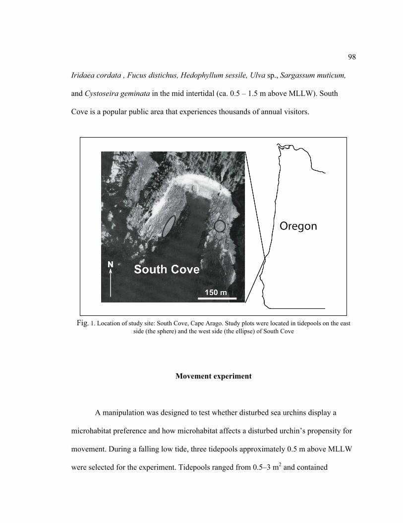
98
Iridaea cordata , Fucus distichus, Hedophyllum sessile, Ulva sp., Sargassum muticum,
and Cystoseira geminata in the mid intertidal (ca. 0.5 – 1.5 m above MLLW). South
Cove is a popular public area that experiences thousands of annual visitors.
Fig. 1. Location of study site: South Cove, Cape Arago. Study plots were located in tidepools on the east
side (the sphere) and the west side (the ellipse) of South Cove
Movement experiment
A manipulation was designed to test whether disturbed sea urchins display a
microhabitat preference and how microhabitat affects a disturbed urchin’s propensity for
movement. During a falling low tide, three tidepools approximately 0.5 m above MLLW
were selected for the experiment. Tidepools ranged from 0.5–3 m2 and contained

99
Strongylocentrotus purpuratus living inside and outside pits. Two tidepools were
completely contained, and one was located in a surge channel, but the tide was low
enough during the experiment that the water was still. Ten haphazardly selected pit
urchins in each tidepool were randomly divided into two treatments: “Inside” and
“Outside”. The sea urchins were disturbed removed from their pits by carefully using a
wide knife as a lever to pry them out. To distinguish between Inside and Outside urchins,
spines were clipped into distinctive patterns with wire-cutters. A large patch of spines
was clipped from one randomly selected treatment group, and two small patches were
clipped from the other treatment group. In case the clipping patterns varied in their
effects on the sea urchins, the treatment groups received each clipping pattern at least
once. Sea urchins were handled for no more than a minute, and then were returned to the
tidepool. Sea urchins in the Inside treatment were returned to their pits, and sea urchins in
the Outside treatment were haphazardly placed in nonpit locations, with the stipulation
that they were at least 10 cm from the nearest empty pit. A sketch made in the field was
used to indicate the position of each sea urchin at the outset of the experiment. After two
hours, before the rising tide reached the pools, the locations of the sea urchins were
noted. The distance of displacement was measured for sea urchins that moved. Three
days later, the tidepools were rechecked and the final microhabitats were noted for sea
urchins in each treatment. Displacement was not measured since I could not distinguish
among the five sea urchins within a treatment.
A chi-square test for a single variable was used to test the H0 that disturbed sea
urchins occurred in a 50:50 ratio in pit and nonpit microhabitats. Rejection of the H0
100
would indicate that one microhabitat was preferred over the other. A two-way
contingency table was used to test the H0 that there is no relationship between treatment
(Inside or Outside) and the occurrence of movement after two hours. Fisher’s Exact Test
was used to correct for small cell counts (Sokal & Rohlf 1995).
Field monitoring of marked plots
At South Cove, a tidepool field monitoring study was used to investigate the
frequency of movement in Strongylocentrotus purpuratus. Its usefulness as a measuring
tool for mortality became apparent as the research was carried out. In June 2005, I
haphazardly selected 21 locations in tidepools to be permanent study plots. To mark the
plots, holes were drilled in the rock and were filled with cylindrical pieces of turquoise
plastic. An original intention of the study was to quantify the number of sea urchins that
evacuate their pits, so while all of the plots had ca. 20–60 pit urchins, they did not
necessarily contain equal numbers of nonpit urchins. Only 3 out of 21 plots initially
contained more nonpit urchins that pit urchins.
The plots were categorized by location in South Cove: East Side Tidepools
(ESTP), West Side Tidepools (WSTP), and West Side Exposed Substrata (WSES). I refer
to these three areas as macrohabitats containing pit and nonpit microhabitats (for
definitions see Chapter II and (Morris 1987). On the east side of South Cove, six ESTP
plots were selected for monitoring. The east side of South Cove is noticeably flatter than
the west side, as it lacks a large boulder and cobble field. Surge channels cut through the
101
sandstone bench, creating many intertidal “islands” that are covered on top with surfgrass
(Phyllospadix scouleri) and are pocketed with small tidepools. Sand accretes in the surge
channels and to a lesser extent the tidepools during the summer months. The plots were in
tidepools about 1 m above MLLW, and plots #5 and #6 were in the same tidepool,
separated by 1 m. Eleven WSTP plots were selected from 0 to 1 m above MLLW. Seven
of these plots were situated in three sections of a very large tidepool. Plots in the same
section (#16–17, #18–20, and #21–22) were spaced 1 m from each other. Rocks emerging
from the tidepool were assumed to reduce the likelihood of movement between sections.
Four WSES plots were not in tidepools, but on rocks projecting from tidepools that were
10–30 cm above the water level at low tide. Plots #9 and #10 were on the same rock,
separated by 1 m.
Field monitoring of Strongylocentrotus purpuratus involved multiple
observations and digital photographs (Canon Powershot S70) of each plot during low
tide. Seaweed obscuring the sea urchins was removed while the photo was taken and
subsequently replaced. I attempted to maintain an identical frame of view in the photos
by orienting the view frame according to the blue plot markers. I made note of any
significant changes in or around the tidepools, including the presence of potential
predators (especially Pycnopodia helianthoides), apparent changes in boulder position,
changes in urchin appearance, etc. The plots could usually be checked in one hour or less.
All plots except two were monitored semi-regularly from 8 June – 23 August
2005 (Summer), and from 27 January – 11 June 2006 (Winter & Spring). Field
monitoring of Plot #2 ceased after 261 days because the plastic markers disappeared and

102
incorrect photos were taken, and field monitoring of Plot #14 ended after 295 days when
the sea urchins were collected for a related growth study. Like most of the North
American Pacific coast, Oregon experiences mixed semi-diurnal tides, and it is only
during spring tidal series that the plots were accessible. Data do not exist for fall 2005
because nighttime low tides, heavy winds, and rain interfered with data collection.
During most tidal series, I made an effort to visit the plots on several consecutive days to
increase the temporal resolution of the study.
The digital photos were downloaded onto a personal computer and viewed with
Adobe Photoshop (Adobe Systems Incorporated 2002). The contrast, brightness, and
color of photos were adjusted so that sea urchins were easily visible. Photos from
consecutive dates were compared and the following data were recorded: 1) the frequency
of each possible change in location (To or From a Pit or Nonpit microhabitat); 2) the
number of sea urchins that had not moved since the beginning of the study; and 3) the
change in the number of sea urchins since the previous photo. The situation sometimes
occurred in which there was a new sea urchin present in a photo, but a sea urchin was
missing from some location in the previous photo. Distinctive rocks and algae held by the
podia, scars, and test diameter were clues that allowed me to determine whether these
were the same or different sea urchins.
The number of pit urchins, nonpit urchins, and empty pits were counted in the
first and final photographs, and a paired student’s t-test was used to test the H0 that there
were no significant differences in these counts between June 2005 and June 2006 (Systat
103
Software, Wilkinson 2004). The paired student’s t-test was also used to compare the
proportion of sea urchins in each microhabitat at the beginning and end of the study.
Changes in the location of sea urchins (To a Pit, From a Pit, To a Nonpit, From a
Nonpit) were summed and expressed as a frequency of movement per urchin per tidal
cycle (urchin changes)(urchin-1
)(tidal series-1
). Standardization to tidal series (i.e., 28
days) resulted in equivalent units for the Summer (75 days of monitoring) and
Winter&Spring (136 days). Movement frequencies were compared within different
seasons and macrohabitats. Separate analyses included only observations taken when 24
hours had elapsed since the previous observation, with the hypothesis that changes in
location on a short time scale were more likely to be due to movement as opposed to
mortality.
RESULTS
Movement experiment
When S. purpuratus were spine-clipped, individuals sometimes appeared
distressed, waving their spines and sometimes displaying pedicillariae. Upon being
returned to the tidepool, the Inside treatment group quickly wedged themselves into the
bottom of their pit, with one exception. Sea urchins in the Outside treatment group,
however, began moving immediately. Within two hours, nine had settled into pits or
104
shallow depressions, two were wedged into crevices in the rock, and only four remained
on flat substrate. After three days, twelve sea urchins Outside pits had moved, but only
one sea urchin Inside pits moved. Results of the field manipulation are displayed in Table
1. The two H0 were rejected. Strongylocentrotus purpuratus in tidepools showed a
preference for pit microhabitats after being disturbed by breaking spines (P < 0.001, c2 =
15.38, df = 1). Sea urchins placed outside pits showed a propensity for movement, while
those inside pits remained in place (P < 0.001, c2 = 16.43, df = 1).
Field monitoring of marked plots
I photographed Strongylocentrotus purpuratus in the permanent intertidal plots
thirteen times each from 9 June – 23 August 2005 and 27 January – 11 June 2006. Field
monitoring occurred on consecutive dates seven times in the Summer season and six
times in the Winter & Spring period. The average number of days between visits was 18
in the Summer and 20 in the Winter & Spring. As few as 9 and as many as 41 days
passed between tidepool visits, in addition to the sampling hiatus between August and
January (155 days).

105
Table 1. Strongylocentrotus purpuratus. The influence of microhabitat on movement of spine-clipped S.
purpuratus. Only the three-day results are displayed, but the two-hour patterns were similar
Pit Nonpit
Observed 23 3
Expected 13 13
c2 = 15.38, df = 1, P < 0.001
The H0 that disturbed S. purpuratus occurs in a 50:50 ratio
in pit and nonpit microhabitats was rejected.
Inside Outside
Moved 1 12
Stayed 14 3
c2 = 16.43, df = 1, P < 0.001
The H0 that there is no relationship between microhabitat and
propensity for movement was rejected.
Sedentary sea urchins and total abundance
Sedentary urchins were those that did not move after field monitoring began. I did
not observe any changes in location for most Strongylocentrotus purpuratus; 637 (93%)
sea urchins were sedentary during the Summer (75 days), and 549 (80%) sea urchins
remained sedentary through the Winter & Spring (367 days). S. purpuratus in WSES
plots were most likely to be sedentary (97% after 75 days; 95% after 367 days). For the
sea urchins present in the plots at the end of the study, I calculated the percentage that
had been sedentary for the previous year (“Sedentary Survivors” in Table 2). About 94%
106
of the sea urchins photographed on 11 June 2006 had not changed position since 9 June
2005. This percentage was similarly high in the three microhabitats, even though
abundances varied greatly.
In June 2005, the 21 intertidal plots contained 688 Strongylocentrotus purpuratus.
One year later, the same plots contained just 583, a decline of 15.3% (Table 2). Sea
urchin abundance decreased at a high rate in ESTP (–25.4%) and WSTP (–14.8%), but
was virtually unchanged in WSES (+1%) (Fig. 2). Some plots experienced a much
greater decline than others in the same macrohabitat. In ESTP, 31 sea urchins
disappeared from Plot #1, while the other five plots had a net loss of 16 urchins. The
ESTP plots were not checked between 25 February and 19 April 2006, during which time
22 urchins in shallow pits disappeared from Plot #1. In WSTP, 44 of 59 missing sea
urchins came from Plots #17 and #18. The decrease in Plot #17 was especially dramatic;
it contained 24 urchins at the beginning of the study and two at the end. Nine urchins
disappeared from this plot during the summer, and another thirteen went missing before
the end of February. The abundance of S. purpuratus in the WSES macrohabitat did not
fluctuate by more than two urchins in any plot (Fig. 2, Table 2).

107
Fig. 2. Strongylocentrotus purpuratus. Total S. purpuratus in 21 plots from 9 June 2005 – 11 June 2006;
Macrohabitats are East Side Tidepools (ESTP), West Side Tidepools (WSTP), and West Side Exposed
Substrata (WSES); no observations were made during 23 August 2005 – 27 January 2006
Microhabitat distribution
The distribution of Strongylocentrotus purpuratus inside and outside pits is
reported for plots in Table 3, and the means (± SE) by macrohabitat are reported in Table
4 and Fig. 3. These tables illustrate two important trends. First, between 2005 and 2006,
there was significant decrease in the number of nonpit urchins (P < 0.01, paired student’s
t-test) but there was no significant difference in the abundance of pit urchins. Second,
although the frequency of pit urchins increased or did not change in every case except
Plot #6 (Table 3), the number of empty pits increased in most plots and was significantly

108
Table 2. Strongylocentrotus purpuratus. Changes in tidepool population of S. purpuratus after 75 days and 1 year; Macrohabitats are East Side Tidepools
(ESTP), West Side Tidepools (WSTP), and West Side Exposed Substrata (WSES); displayed is the initial, final, and change in total urchins for each plot,
percentage of S. purpuratus that were sedentary for 75 days and 1 year, and the percentage of surviving S. purpuratus that had been sedentary for one year;
sedentary urchins appeared in the same location in every photo
Total S. purpuratus Sedentary for 75 days Sedentary for one year
Macrohabitat Plot # 9 June 2005 11 June 2006 Change % Total % Total % Survivors
ESTP 1 52 21 -31 -60 47 90 21 40 100
2 18 14 -4 -22 14 78 13 72 93
3 17 13 -4 -24 15 88 12 71 92
4 28 23 -5 -18 27 96 22 79 96
5 34 31 -3 -9 34 100 31 91 100
6 36 36 0 0 35 97 32 89 89
WSTP 10 33 34 +1 +3 29 88 29 88 85
12 64 60 -4 -6 62 97 59 92 98
14 30 26 -4 -13 26 87 26 87 100
15 19 19 0 0 18 95 17 90 89
16 46 49 +3 +7 46 100 43 93 88
17 24 2 -22 -92 15 63 1 4 50
18 53 31 -22 -42 46 87 27 51 87
19 28 24 -4 -14 26 93 24 86 100
20 41 40 -1 -2 40 98 38 93 95
21 34 33 -1 -3 32 94 32 94 97
22 28 23 -5 -18 25 89 22 79 96
WSES 8 26 28 +2 +8 26 100 26 100 93
9 36 36 0 0 35 97 35 97 97
11 22 23 +1 +5 21 96 21 91 91
13 19 17 -2 -11 18 95 17 89 100
All plots 688 583 -105 -15.3 637 92.6 549 79.8 94.2
ESTP 185 138 -47 -25.4 172 93.0 131 70.8 94.9
WSTP 400 341 -59 -14.8 365 91.3 318 79.5 93.3
WSES 103 104 +1 +1.0 100 97.1 99 96.1 95.2
Sedentary
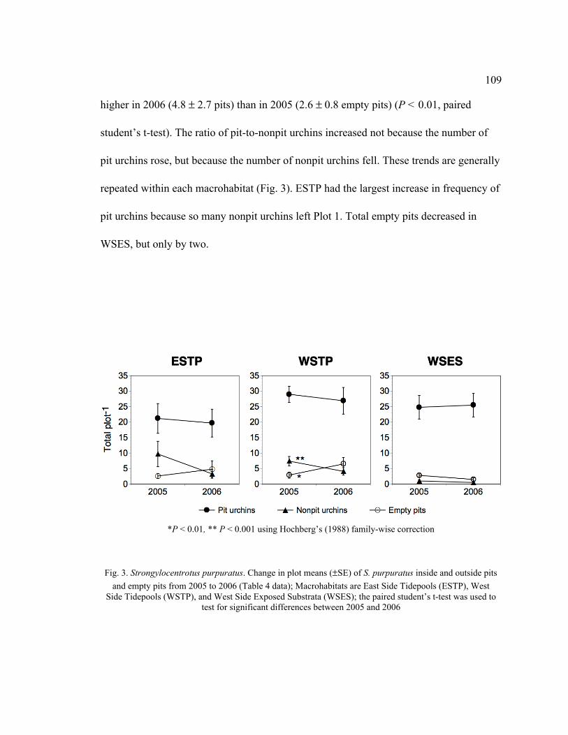
109
higher in 2006 (4.8 ± 2.7 pits) than in 2005 (2.6 ± 0.8 empty pits) (P < 0.01, paired
student’s t-test). The ratio of pit-to-nonpit urchins increased not because the number of
pit urchins rose, but because the number of nonpit urchins fell. These trends are generally
repeated within each macrohabitat (Fig. 3). ESTP had the largest increase in frequency of
pit urchins because so many nonpit urchins left Plot 1. Total empty pits decreased in
WSES, but only by two.
*P < 0.01, ** P < 0.001 using Hochberg’s (1988) family-wise correction
Fig. 3. Strongylocentrotus purpuratus. Change in plot means (±SE) of S. purpuratus inside and outside pits
and empty pits from 2005 to 2006 (Table 4 data); Macrohabitats are East Side Tidepools (ESTP), West
Side Tidepools (WSTP), and West Side Exposed Substrata (WSES); the paired student’s t-test was used to
test for significant differences between 2005 and 2006
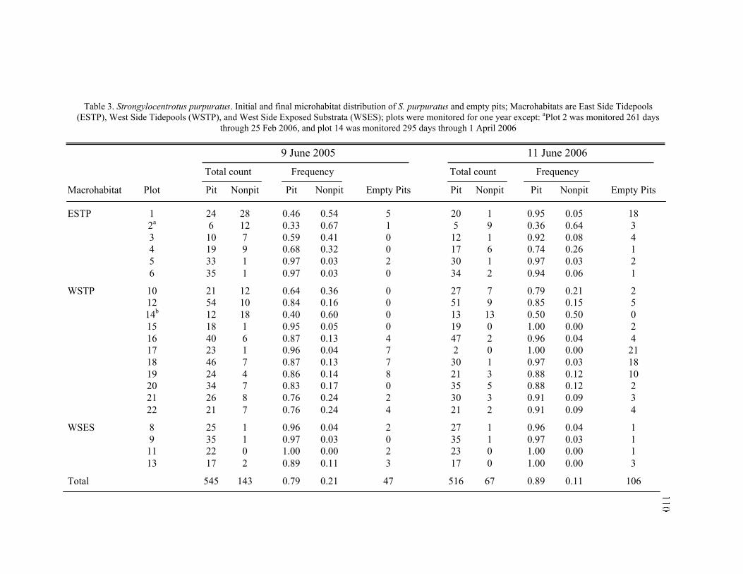
Table 3. Strongylocentrotus purpuratus. Initial and final microhabitat distribution of S. purpuratus and empty pits; Macrohabitats are East Side Tidepools
(ESTP), West Side Tidepools (WSTP), and West Side Exposed Substrata (WSES); plots were monitored for one year except: aPlot 2 was monitored 261 days
through 25 Feb 2006, and plot 14 was monitored 295 days through 1 April 2006
9 June 2005 11 June 2006
Total count Frequency Total count Frequency
Macrohabitat Plot Pit Nonpit Pit Nonpit Empty Pits Pit Nonpit Pit Nonpit Empty Pits
ESTP 1 24 28 0.46 0.54 5 20 1 0.95 0.05 18
2a
6 12 0.33 0.67 1 5 9 0.36 0.64 3
3 10 7 0.59 0.41 0 12 1 0.92 0.08 4
4 19 9 0.68 0.32 0 17 6 0.74 0.26 1
5 33 1 0.97 0.03 2 30 1 0.97 0.03 2
6 35 1 0.97 0.03 0 34 2 0.94 0.06 1
WSTP 10 21 12 0.64 0.36 0 27 7 0.79 0.21 2
12 54 10 0.84 0.16 0 51 9 0.85 0.15 5
14b
12 18 0.40 0.60 0 13 13 0.50 0.50 0
15 18 1 0.95 0.05 0 19 0 1.00 0.00 2
16 40 6 0.87 0.13 4 47 2 0.96 0.04 4
17 23 1 0.96 0.04 7 2 0 1.00 0.00 21
18 46 7 0.87 0.13 7 30 1 0.97 0.03 18
19 24 4 0.86 0.14 8 21 3 0.88 0.12 10
20 34 7 0.83 0.17 0 35 5 0.88 0.12 2
21 26 8 0.76 0.24 2 30 3 0.91 0.09 3
22 21 7 0.76 0.24 4 21 2 0.91 0.09 4
WSES 8 25 1 0.96 0.04 2 27 1 0.96 0.04 1
9 35 1 0.97 0.03 0 35 1 0.97 0.03 1
11 22 0 1.00 0.00 2 23 0 1.00 0.00 1
13 17 2 0.89 0.11 3 17 0 1.00 0.00 3
Total 545 143 0.79 0.21 47 516 67 0.89 0.11 106

Table 4. Strongylocentrotus purpuratus. Initial and final plot means (±SE) and frequency of S. purpuratus inside and outside pits and empty pits per plot;
Macrohabitats are East Side Tidepools (ESTP), West Side Tidepools (WSTP), and West Side Exposed Substrata (WSES); the paired student’s t-test was used
to check for significant differences between 2005 and 2006
9 June 2005 11 June 2006
Total count Frequency Total count Frequency
Macrohabitat Pit Nonpit Pit Nonpit Empty Pits Pit Nonpit Pit Nonpit Empty Pits
ESTP 21.2 ± 4.8 9.7 ± 4.1 0.69 0.31 2.6 ± 0.8 19.7 ± 4.5 3.3 ± 1.4 0.86 0.14 4.8 ± 2.7
WSTP 29.0 ± 2.6 7.4 ± 1.5 0.80 0.20 2.9 ± 1.0 26.9 ± 4.3 4.1 ±1.2 0.87 0.13 6.5 ± 2.1
WSEP 24.8 ± 3.8 1.0 ± 0.4 0.96 0.04 2.8 ± 0.5 25.5 ± 3.8 0.5 ± 0.3 0.98 0.02 1.5 ± 0.5
Total 26.0 ± 2.6 6.8 ± 1.5 0.79 0.21 2.1 ± 0.6 24.6 ± 2.7 3.2 ± 0.8 0.89 0.11 5.0 ± 1.4
Paired t-test NS * ** * *
between years
*P < 0.01, ** P < 0.001 using Hochberg’s (1988) family-wise correction
112
Movement frequency by microhabitat
Changes in the location of sea urchins could be categorized four ways: To a Pit,
From a Pit, To a Nonpit, or From a Nonpit. The frequencies of each change in location
for macrohabitats and seasons are displayed in Fig. 4. Sea urchins tended to move From a
location more frequently than To a location in a plot, agreeing with the general decline in
sea urchin abundance between plots. The location of sea urchins in the WSES
macrohabitat changed least frequently (Fig. 4). There were more than 0.1 changes From a
Pit (urchin-1
)(plot-1
) during Winter & Spring in ESTP, and during both seasons for
WSTP. The only other instance in which there were at least 0.1 changes in location
(urchin-1
)(tidepool-1
) was To a Pit during Winter & Spring in ESTP.
More changes in location were detected when more days elapsed between
observations (Fig. 5). Changes in urchin location plot-1
and urchin-1
were about four times
higher after more than nine days compared to one day. After one day, there was a mean
(± SE) of 0.008 ± 0.002 changes in location urchin-1
, which is equivalent to 0.231 ± 0.047
changes (urchin-1
)(tidal series-1
). This means that during a given tidal series, about one of
four sea urchins would be expected to show a change in location. Fig. 6 displays the
frequencies of changes in location within each macrohabitat when sea urchins were
observed on consecutive days. The amount of movement in and out of pits was about
twice as great as the movement to and from nonpit locations.

113
Fig. 4. Strongylocentrotus purpuratus. Microhabitat-specific changes in urchin locations during Summer (9
June – 23 August 2005) and Winter & Spring (27 January – 11 June 2006); units for appearances and
disappearances are (changes in location)(urchins-1
)(tidal series-1
); Macrohabitats are East Side Tidepools
(ESTP), West Side Tidepools (WSTP), and West Side Exposed Substrata (WSES); error terms are SE
Fig. 5. Strongylocentrotus purpuratus. Mean (± SE) changes in sea urchin location when checking plots
after 1 day or >9 days; sea urchins observed to change locations were 68 after 1 day and 197 after >9 days;
units for change in location is in bold type above figure; >9 days group had a range of 9 – 41 with mean
19.4 days; *this value is severely underestimated because temporal resolution for the >9 day group is so
low; these data were collected after an average of 19 days, so many instances of urchin movement may
have gone undetected
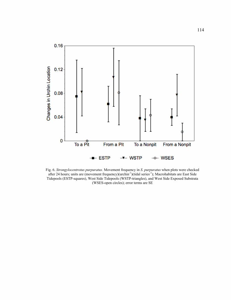
114
Fig. 6. Strongylocentrotus purpuratus. Movement frequency in S. purpuratus when plots were checked
after 24 hours; units are (movement frequency)(urchin-1
)(tidal series-1
); Macrohabitats are East Side
Tidepools (ESTP-squares), West Side Tidepools (WSTP-triangles), and West Side Exposed Substrata
(WSES-open circles); error terms are SE

115
DISCUSSION
A sedentary lifestyle in Strongylocentrotus purpuratus
The major limitation of this study is my inability to accurately distinguish
movement from mortality. The presence and subsequent absence of a sea urchin in a
series of photos could mean that the animal moved or died. However, I can deduce that a
sea urchin had not moved when its location was unchanged. In every set of photos, most
individuals appeared in the exact same location repeatedly. Often, unmoving sea urchins
in successive photos even held the same rocks and pieces of algae for days at a time.
Over the course of this study, most sea urchins were never observed to move. An
astonishing 94% of the sea urchins appearing in the final set of plot photos had been
sedentary for the length of the one-year study. The data provide overwhelming evidence
that Strongylocentrotus purpuratus tends to live a sedentary lifestyle at South Cove.
This finding adds weight to my previous conclusions concerning morphology and
growth in Strongylocentrotus purpuratus. At three sites, morphological distinctions were
made between sea urchins living in different microhabitats (see Chapter II). Pit urchins
had relatively taller tests and larger Aristotle’s lanterns, while nonpit urchins had greater
test diameters, spine length, and skeletal mass. Nonpit urchins also had higher growth
rates than pit urchins (see Chapter III). The interpretation that microhabitat-use leads to
the observed differences in morphology and growth inherently assumes that most sea
urchins do not frequently switch microhabitats. This study, which detected extensive
116
sedentary behavior in S. purpuratus, supports the hypothesis of consistent microhabitat-
use and validates the partitioning of pit urchins and nonpit urchins.
Despite the high frequency of sedentary behavior displayed by intertidal sea
urchins, some individuals in the plots obviously moved. Observation of the presence
followed by the absence of a sea urchin in a photo could be the result of movement or
mortality, but how can the two be distinguished? The most accurate measure of
movement frequency comes from the data collected on successive days. If I was present
at South Cove during low tide, terrestrial predators were unable to forage on sea urchins.
The sunflower sea star (Pycnopodia helianthoides), the only known marine predator that
consumes sea urchins at South Cove, could still forage at high tide, but then I probably
would have seen them near the plots during the following low tide. Since I only observed
P. helianthoides a few times near Plots #17 and #18, I presume that when the location of
sea urchins changed after one day, movement was the cause. There were 12 – 14 plot
observations made one day after the previous observation (depending on the plot). In
these instances, there was a mean of 0.231 ± 0.047 movements (urchin-1
)(tidal series-1
)
(Fig. 5). Therefore, after four tidal series (16 weeks), one would expect approximately
one occurrence of movement per urchin.
Fig. 6 indicates that movement frequency was greater for pit urchins than for
nonpit urchins. Since pit urchins were much more numerous than nonpit urchins (Table
3), individual movement rates were actually greater in nonpit microhabitats. A
manipulation demonstrated that pits were the “preferred” microhabitat when the spines of
117
a sea urchin had been clipped. These results that individual behavior may be related to
microhabitat; sea urchins inside pits are less likely to move than those outside pits.
Yusa and Yamamoto (1994) also reported a difference in echinoid movement
related to microhabitat. They investigated Anthocidaris crassispina, which, like S.
purpuratus, occurs inside and outside of pits in tidepools. A. crassispina inside pits never
moved, but outside pits they were highly mobile. When sea urchins were switched into
the opposite microhabitat, they altered their movement patterns accordingly; urchins
outside pits still moved much more than those inside pits. In the present study, the
conclusion of a sedentary lifestyle is appropriate for pit urchins, which account for most
of the individuals observed. More data are needed to demonstrate the same for nonpit
urchins. A field observation involving Lithothammnium sp., a coralline encrusting algae,
lends some support to the sedentary lifestyle hypothesis for sea urchins in both
microhabitats. In tidepools with high urchin densities, substratum between urchins is
often covered with Lithothamnium. Removing a nonpit urchin from the rock reveals a
bare patch, identifying that position as a home scar that the sea urchin has scraped clean
of algae. If nonpit urchins were mobile, additional bare patches and scrapes of the algae
would indicate their grazing activity. The unbroken algal crust in some tidepools may be
a sign of sedentary behavior in Strongylocentrotus purpuratus in different microhabitats.
Habitation of pits (also “crevices,” “cavities,” or “burrows”) is a common
behavior in various species of sea urchins in temperate (Otter 1932, Lissner 1980,
Kawamata 1998) and tropical regions (Grünbaum et al. 1978, Carpenter 1984, Neill
1988, Schoppe & Werding 1996). Many echinoids move out of their burrows at night to
118
forage and return to their protective microhabitats before dawn (Grünbaum et al. 1978,
Nelson & Vance 1979), while other studies did not observe movement out of burrows
(Otter 1932, Maier & Roe 1983, Tsuchiya & Nishihira 1985, Yusa & Yamamoto 1994,
Schoppe & Werding 1996). Predation has been implicated as a cause for homing
behavior in sea urchins that forage outside their pits (Carpenter 1984, Neill 1987), and
McClanahan (1999) used tethering experiments to show that predators restrict
Echinometra viridis to crevices during daylight hours. The lack of observed movement in
Strongylocentrotus purpuratus does not preclude nocturnal foraging as a common
behavior, but considering the high densities of sea urchins in many tidepools (>100 m-2
),
it seems highly unlikely that each individual could move around at night and manage to
reoccupy its own pit during the day. The ability to home precisely in such high densities
would be quite an unexpected discovery.
The lack of mobility in Strongylocentrotus purpuratus is likely related to the
habitat in which they are found. The risk of dislodgement is at least 50% when water
velocity is greater than 17 m s-1
(Denny & Gaylord 1996), and velocities have been
measured in excess of 25 m s-1
on exposed rocky shorelines (Denny et al. 2003). Several
studies have demonstrated that movement in sea urchins is negatively correlated with
water velocity. Kawamata (2001) reported that movement rates were reduced by half
when water velocity was 0.4 m s-1
, and movement became nearly impossible when water
velocity was increased to 0.7 m s-1
. Likewise, under calm ocean conditions, the sea urchin
Centrostephanus coronatus always emerges from its burrows at night at depths of 5 m
(Lissner 1980). It was only when seas became rough that many sea urchins became
119
sedentary. Though aggregations of mobile grazing S. purpuratus have been observed in
the subtidal (Harrold & Reed 1985), the extreme wave velocities and hydrodynamic
forces that assail the shoreline might prevent similar behavior in intertidal populations of
S. purpuratus.
Frank (1981) described the conditions that might make a sedentary lifestyle
adaptive in an organism capable of mobility. While observing oystercatchers forage on
limpets in Middle Cove of Cape Arago, 1 km from the site of this study, he discovered
that most limpets on horizontal surfaces were eaten (Frank 1982). Meanwhile, limpets on
vertical surfaces were still abundant, having been restricted to locations inaccessible to
the oystercatchers. While the limpets studied were mobile grazers, their foraging paths
led them back near their original starting place (imperfect homing), so from the
perspective of a terrestrial predator, they were essentially unavailable. Frank (1981)
proposed that sedentary or homing behavior might be adaptive when: 1) food is locally
available; and 2) there are long-lasting, significant differences in survivorship between
patches, so that an organism is benefited by remaining in its habitat patch permanently. In
this study, Strongylocentrotus purpuratus displayed secondary sedentary behavior,
meaning that although capable of moving, they stay in one place. As feeders of drift
algae, they fulfill the first of Frank’s criteria for adaptive sedentary behavior. To fully test
his hypothesis, mortality would need to be clearly linked to movement, which this study
was not designed to accomplish. However, one year of field-monitoring led to several
findings related to mortality.
120
Movement or mortality?
Mortality was a confounding factor that sometimes made it impossible to infer
movement when a sea urchin disappeared from a plot photo, as it could have moved or
died. A change in abundance (as measured by the sum of sea urchins in all plots) could be
due to recruitment, immigration into or emigration out of plots, or mortality. If
recruitment of Strongylocentrotus purpuratus had been heavy in recent years, juveniles
increasing in size and becoming more visible may have confounded the results. Since
recruitment has been weak at South Cove for at least four years (see Chapter III), hard-to-
see small urchins were not problematic. If immigration and emigration rates were not
equal for the study plots, my counts of total abundance would be affected. Assuming that
habitat inside and outside plots is comparable, there is no reason that moving urchins
should be more likely to immigrate to or emigrate from the plots, so I would not expect
movement to influence overall abundance. This study suggests that mortality in the
tidepools was approximately 15%, equal to the proportion of sea urchins that went
missing from the marked plots during the year of field monitoring. This rough estimate,
based on the disappearance of about 100 sea urchins from plots covering a fraction of
South Cove, agrees nicely with data from other populations of S. purpuratus. Russell
(1987) measured z (mortality rate) to range from 0.12–0.33 in San Diego, California and
from 0.10–0.16 on Vancouver Island. Of the two locations, the climate and
oceanographic conditions in Oregon are more similar to Vancouver, and my estimate for
mortality falls in line with Russell’s maximum estimate.
121
Decreases in abundance of Strongylocentrotus purpuratus were detected in nearly
every plot and varied greatly between plots. Specifically, sea urchins in plots #1, #17, and
#18 were most likely to move or die, and together these plots accounted for 71% of the
total decrease in abundance. A possible explanation for higher movement/mortality in
these plots comes from extensive field observations. From January–August 2006, I
observed considerable predation on sea urchins by Pycnopodia helianthoides, American
black oystercatchers (Haematopus bachmani), and raccoons (Procyon lotor) (discussed in
detail in Chapter V). The east side of South Cove, where Plot #1 was located, was the
central foraging area of at least six oystercatchers and two raccoons. Both predators are
able to consume over 35 sea urchins during a single low tide, so it is not hard to believe
that they would eventually forage in the monitoring plots. Additionally, two months after
the monitoring period ended, the remaining thirteen sea urchins in Plot #3 went missing.
Plots #1 and #3 are shallow pools on tall sandstone benches surrounded by the surfgrass
Phyllospadix scouleri. It is more probable that these plots were discovered by foraging
raccoons or oystercatchers than every urchin evacuated the tidepools and moved into the
surfgrass (Laur et al. 1986).
Plots #17 and #18 were located in a large, mid intertidal pool on the west side of
South Cove. Though the tidepool contained hundreds, if not thousands of
Strongylocentrotus purpuratus, I never observed any terrestrial predators near it. One
Pycnopodia helianthoides, however, was observed in August 2005 and on several
occasions thereafter, usually at the deepest part of the tidepool underneath surfgrass. This
sea star, which has been observed to specialize on S. purpuratus in the rocky intertidal
122
(Mauzey et al. 1968, Dayton 1975), is likely responsible for the missing sea urchins in
Plots #17 and #18, which were closest in proximity to the P. helianthoides. Unlike
oystercatchers and raccoons, P. helianthoides only eats one sea urchin per day, but S.
purpuratus usually reacts to its presence by moving away from it relatively quickly
(Dayton 1975). If many of the sea urchins that disappeared from these plots were chased
away instead of eaten, then I may be overestimating predation in my estimate based on
urchin abundance in study plots.
The number of nonpit urchins decreased more than the number of pit urchins,
which were much more common. Nonpit urchins could be more susceptible to predation
than pit urchins, but other sources of mortality might be more likely to kill nonpit urchins
without harming pit urchins. During winter storms, strong surges produce acceleration
forces strong enough to move boulders and slam cobble into the substratum with enough
force to influence the distribution of barnacles, limpets, and other species (Dayton 1971,
Shanks & Wright 1986, van Tamelen 1996). Some of these wave-borne projectiles may
collide with and damage the tests of sea urchins. At South Cove, about 9% of tests from
sacrificed sea urchins had damage marks, indicating that living sea urchins underwent
recalcification to repair dents or breaks in their test plates. Sea urchins lacking protective
pits would seem especially subject to damage from wave-borne projectiles, which
probably leads to mortality more often than successful test repair. Even deadlier than a
flung cobble would be a rolling boulder. In one tidepool at South Cove, a large (ca. 0.5
m3) boulder was found to have moved several meters during the winter, narrowly
avoiding the sea urchins in Plot #14. Using a crowbar as a lever, I lifted the boulder to
123
find sea urchins underneath it that survived, protected inside their pits. This anecdotal
evidence suggests that survivorship in intertidal Strongylocentrotus purpuratus is
enhanced by protective pits in the substrata.
Conclusion
One year of field monitoring and a short-term manipulation study were used to
investigate movement and mortality in Strongylocentrotus purpuratus. The primary
finding was that movement was very infrequent in an intertidal population of S.
purpuratus at South Cove, Cape Arago. About 94% of the sea urchins present at the end
of the study were not observed to move during the year; thus they were sedentary. A field
manipulation indicated that disturbed S. purpuratus utilize pit microhabitats as refuges,
and observations of movement suggested that nonpit urchins might be more likely to
move than pit urchins. Extreme water velocities encountered in the intertidal might
present a high risk of dislodgement that is ameliorated in when a sea urchin remains
sedentary inside a pit. The total abundance of S. purpuratus was observed to decline by
15% during the year, from 688 to 583 individuals. A large part of this decline was
probably due to mortality resulting from predation. Movement out of plots may also have
contributed to the change in abundance, but most individuals were sedentary, reducing
the likelihood that emigration from pits played a significant role. Nonpit urchins
decreased more than pit urchins, suggesting that microhabitat use affects mortality. A
positive trade-off associated with living in a more dangerous environment outside a pit

124
could be an increased growth rate (see Chapter III). Nonpit urchins grow faster than pit
urchins and attain a larger size, so although they might be more likely to perish, nonpit
urchins may have greater reproductive output than pit urchins.

125
Bridge to Chapter V
Though this chapter focuses on the sedentary habits of Strongylocentrotus
purpuratus, it is the infrequent observations of movement that actually address the major
question at hand. Technically, if each sea urchin moved only once in its life, but tended to
move out of pits, then nonpit urchins would be larger than pit urchins, as indicated in
Chapter III. If sea urchins live an average of 16 years, and 6% of the population moves
once in a year, then each urchin would move on average one time during its life. These
averages are quite similar to the observations from South Cove. So while I have not
proven that movement out of pits accounts for the microhabitat-based difference in size
structure, I also cannot reject the hypothesis. Combined with the effects of differential
growth, movement seems a likely mechanism to produce the bimodal distribution.
However, one hypothesis remains, that dealing with differential mortality.
Chapter V is the result of diligence and nature’s serendipity. One cannot truly understand
a habitat until he has experienced it frequently and seasonally. Over the past two years, I
feel I have just begun to understand the ecology of South Cove and particularly its sea
urchins. In 2006, a unique predation event occurred at this site, and the resulting unequal
microhabitat effects contributed another piece to this puzzle.
There once was an urchin named June
Who crawled out of a tidepool at noon.
She thought she was safe
Far from stars and big waves,
But she just didn’t count on raccoons.

126
CHAPTER V
STAMPEDING SEA URCHINS AND INDIRECT EFFECTS IN AN
INTERTIDAL FOOD WEB
INTRODUCTION
Ecologists characterize interspecific relationships based on changes in the
abundances or densities of species resulting from interactions. Direct effects such as
predation, competition, grazing, and mutualisms involve only two species. When one
species influences another by interacting with a third species, the interaction is said to be
one of indirect effects (Menge & Branch 2001). For example, on New England’s rocky
shores, the snail Littorina littorea is an important grazer that structures tidepool algal
communities (Lubchenco 1978). When the predatory green crab Carcinus maenas
reduces the density of L. littorea, positive indirect effects are passed on to the algae that
are released from grazing pressure. Predation alone is not responsible for reducing snail
density, as was first believed. When L. littorea detects the presence of C. maenas, it
moves away from the predator evacuating the tidepool. This fleeing response reduces
grazing pressure more than the direct effects of the predator, which in this case may be
negligible (Trussell et al. 2004). The indirect effects of C. maenas on the tidepool algae
are trait-mediated, that is, they result from L. littorea changing its behavior in response to
127
a detected predator (Schmitz et al. 2004). Brown (1999) suggested that understanding the
role of “fear” should be central to the study of species interactions. In an effort to avoid
predation, herbivores may flee predators as in the case of Littorina littorea, resulting in
reduced density.
A shift in behavior can also produce cascading effects in the community. Two
species of sea urchins (Strongylocentrotus droebachiensis and S. franciscanus) altered
their grazing rates when exposed to the chemical cue of a predatory sea star (Pycnopodia
helianthoides) (Freeman 2005). Like C. maenas, simply the presence of P. helianthoides
may benefit the algal community by causing the herbivores to flee. Trait-mediated
interactions cannot always be measured by trophic cascades. Kiesecker and Blaustein
(1998) used experimental pools to expose larval red-legged frogs (Rana aurora) to
different combinations of predators. No predator by itself had a significant effect on the
tadpoles; when bullfrogs were added to the pools, R. aurora moved deeper, and when
smallmouth bass were added to the pools, R. aurora moved into the shallows. When both
predators were placed in the pools, however, R. aurora experienced significant mortality.
R. aurora’s trait-mediated response to one predator made it more susceptible to the other.
The effects of multiple predators on a population of purple sea urchins
(Strongylocentrotus purpuratus) were investigated in Oregon. The predators included one
invertebrate, the sunflower sea star Pycnopodia helianthoides (hereafter Pycnopodia) and
two terrestrial predators, the raccoon (Procyon lotor) and the American black
oystercatcher (Haematopus bachmani). Of the three, Pycnopodia is the best-known
predator of sea urchins (Mauzey et al. 1968, Dayton 1973, 1975, Moitoza & Phillips
128
1979, Tegner & Dayton 1981, Duggins 1983, Lafferty & Kushner 2000), while the
behavior is less common in raccoons (Carlton & Hodder 2003) and oystercatchers (Falxa
1992, Wootton 1997).
Oystercatchers, especially the European species (Haematopus ostralegus) have
been the subjects of many studies investigating foraging behavior (O'Connor & Brown
1977, Wanink & Zwarts 1985, Meire & Ervynck 1986, Leopold et al. 1996). Several
studies have demonstrated that oystercatchers display aspects of optimal foraging
behavior, in which energy gain is maximized and energy loss is minimized (Stephens &
Krebs 1986). Oystercatchers select prey that is larger than what is most commonly
available (Hartwick 1976, Goss-Custard 1996), and they make economic decisions when
foraging, selecting prey that offer the most energy per unit effort (Wanink & Zwarts
1985, Meire & Ervynck 1986).
Thirty years ago, Dayton (1973, 1975) described a combination of direct and
indirect interactions that resulted from several years of field observations in rocky
intertidal regions of Washington. At one particular site, Dayton noted that a Pycnopodia
occasionally entered a tidepool densely packed with purple sea urchins. The urchins
immediately responded to the presence of Pycnopodia by exposing defensive
pedicillariae and moving away, often over the backs of their neighbors. Within weeks to a
few months, tidepools were completely cleared of sea urchins, and the bare substrate was
soon colonized by algal settlers. Dayton called this phenomenon “urchin stampeding.”
The stampeding urchins, now holding onto the spines of other urchins instead of rocks,
were not able to maintain their grip when exposed to strong waves, and after being swept
129
into the surf, many were caught and consumed by the giant green anemone Antheopleura
xanthogrammica. The number of sea urchins consumed by the sea anemones was
probably an order of magnitude greater than those consumed by Pycnopodia, which eats
only one urchin per 24–48 hours (Dayton 1973). In this example, the indirect effects
(urchin stampeding) of Pycnopodia are greater than its direct effects (predation).
Pycnopodia can eat at most one sea urchin per day, but it caused hundreds of sea urchins
to stampede out of tidepools to their death. A. xanthogrammica benefited from the trait-
mediated behavior displayed by the sea urchins, since they obtained much more food
when Pycnopodia was foraging nearby (Dayton 1973).
Beginning in early 2006, at Cape Arago in southern Oregon, I observed a similar
situation in which the presence of Pycnopodia resulted in large stampedes of purple sea
urchins. The primary beneficiaries of Pycnopodia’s indirect effects in this scenario,
however, were black oystercatchers and raccoons. I describe the foraging behaviors of all
three predators and estimate the overall effect on the local sea urchin population. An
opportunity was presented to compare interspecific direct effects when each predator was
observed foraging in the same area at South Cove. Finally, I compare the sea urchin
population structure to the death assemblages preyed on by oystercatchers and raccoons.
The various abundances, behaviors, and foraging strategies of the predators necessitated
the utilization of different methods of data collection for Pycnopodia, oystercatchers, and
raccoons. Descriptions of field observations, foraging behaviors, and data are contained
in the results.
130
MATERIALS AND METHODS
Study site
All observations and data were collected at South Cove of Cape Arago
(43o18.5’N, 124
o24’W) (Fig. 1), a prominent headland in southern Oregon, USA. Cape
Arago is exposed to large swells and strong winds associated with winter storms, but
South Cove is otherwise fairly protected. The U-shaped cove has a sandy beach flanked
by two intertidal sandstone benches. The west side of South Cove (hereafter: West Side)
is a cobble- and boulder field that gradually slopes toward the water. Near the opening of
the cove (the black outline in Fig. 1A), the intertidal becomes slightly more exposed,
macroalgal growth is profuse in the growing season (e.g., Nereocystis luetkeana, Alaria
marginata, Iridaea cordata, Fucus distichus, Hedophyllum sessile, Egregia menziesii,
Ulva sp., Sargassum muticum, Cystoseira geminata), and purple sea urchins occur in
large tidepools and on sandstone benches. This extensive population of sea urchins
covers most available surface from approximately 0.75 m above mean lower low water
(MLLW) to 0.3 m below MLLW. Many of the sea urchins are situated inside depressions
they excavate from the rock (see Chapter II). Special attention was given to four large
tidepools, denoted H, I, J, and K, where urchin stampeding in 2006 was first observed.
Tidepool H was approximately 5 m2 in area, tidepool J was approximately 8 m
2 in area,
and tidepools I and K were approximately 15 m2 in area. Tidal height was 0 MLLW for
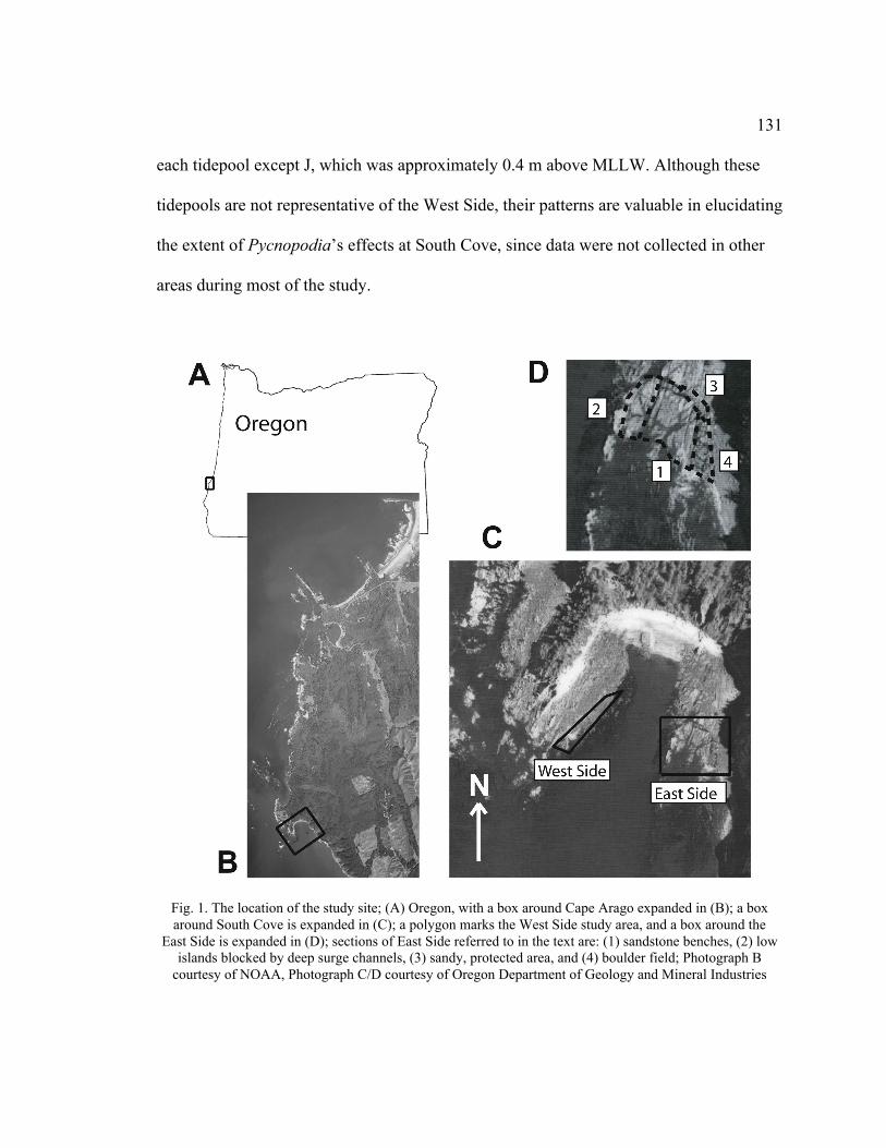
131
each tidepool except J, which was approximately 0.4 m above MLLW. Although these
tidepools are not representative of the West Side, their patterns are valuable in elucidating
the extent of Pycnopodia’s effects at South Cove, since data were not collected in other
areas during most of the study.
Fig. 1. The location of the study site; (A) Oregon, with a box around Cape Arago expanded in (B); a box
around South Cove is expanded in (C); a polygon marks the West Side study area, and a box around the
East Side is expanded in (D); sections of East Side referred to in the text are: (1) sandstone benches, (2) low
islands blocked by deep surge channels, (3) sandy, protected area, and (4) boulder field; Photograph B
courtesy of NOAA, Photograph C/D courtesy of Oregon Department of Geology and Mineral Industries

132
The east side of South Cove (hereafter East Side), lacking a large boulder and
cobble field, has a markedly flatter topography than the West Side. Intertwining surge
channels cut the sandstone bench into intertidal “islands” about 1 m above MLLW that
are pocketed with tidepools and covered on top by the surfgrass Phyllospadix scouleri.
High densities of sea urchins are found on shorter benches up to 0.5 m above MLLW, but
they are most abundant at or below MLLW. Many of the urchins are wedged inside
excavated pits (see Chapter II), especially those on the sides of surge channels, which in
which sand accretes during the summer. The lower distributional limit for sea urchins
seems to be about 0.5 m below MLLW. The low benches do not contain surfgrass, but
brown, filamentous algae (Sargassum muticum and Cystoseira geminata) are common on
vertical surfaces and adjacent to tidepools packed with sea urchins. The macroalgal
community on the East Side is not as dense or speciose as the west side. Laminaria
setchelli is well established throughout surge channels and the shallow subtidal, and
Egregia menziesii is common below MLLW. On both sides of South Cove, where sea
urchins cover extensive portions of the substrate, macroalgal growth is restricted to the
tops and sides of rocks. An intertidal boulder field begins on the landward side of the
benches and follows the coastline south out of the cove.
Sea urchin density
The frequency of data collection depended on the tidal cycles; Oregon and most
of the North American West Coast experience mixed semidiurnal tides, so it was only
133
during daylight low tides below 0 m MLLW that study areas were emergent. During a
particularly low tide in May 2006, the density of sea urchins was measured with belt
transects. On the West Side, I counted all the sea urchins in three random transects 1 m
wide and 20–25 m long, extending from approximately 0.3 m below MLLW, the lower
boundary for sea urchins at that location, to the upper boundary 0.75 m above MLLW.
On the East Side, urchins in three transects with random origins along the northern edge
of the sandstone benches were counted (see Fig. 1D). Transects were 1 m wide and
extended 24, 29, and 49 m across the benches and surge channels. Density was calculated
as total sea urchins divided by the total transect area, including surge channels. The total
area of the sites (black polygons in Fig. 1C) was calculated using overhead aerial
photographs (Oregon Department of Geology and Mineral Industries) and ImageJ
(Rasband 2006). In addition, the size structure of the sea urchin population was sampled
by measuring the test diameters to the nearest 0.1 cm of all the sea urchins in 24
randomly placed quadrats.
Predation by Pycnopodia
The number of intertidal purple sea urchins consumed by Pycnopodia in South
Cove was estimated by modifying a rate of prey removal equation presented by Birkeland
(1974) and utilized by Duggins (1983) for Pycnpodia predation. The rate of sea urchins
consumed Pycnopodia-1
day-1
was calculated as:

134
�
U
I
Ê Ë
ˆ ¯ W
Y(1)
where I is the number of Pycnopodia eating or digesting U sea urchins, W is the rate of
successful attacks, and Y is the digestion time (in days) of one sea urchin. This equation
was multiplied by 365 to yield the number of consumed sea urchins Pycnopodia-1
year-1
.
Multiplying this value by the intertidal population of Pycnopodia (P) in South Cove gave
the estimate of annual predation for the population:
�
365U
I
Ê Ë
ˆ ¯ WP
Y
.(2)
P was calculated by counting Pycnopodia at South Cove several times from
February through August 2006. In February on the West Side, tidepools H–K were
thoroughly searched for Pycnopodia; in April and May, tidepools I–K were searched. In
August, I examined the entire mid and lower intertidal of the West Side, counting all
Pycnopodia at a tidal height of 0.2 m below MLLW and higher. On the East Side at the
same tidal heights, I counted all the Pycnopodia I could find in May, July, and August
2006.
Over the course of a spring tidal series in August, Pycnopodia were inspected to
determine how many were eating purple sea urchins. Once a Pycnopodia has ingested its
food, it is difficult to remove it without injuring the animal. The test of a sea urchin,
however, creates a telltale bulge so that Pycnopodia can be checked for urchin predation
without harming them. If possible, individuals were flipped over to check for prey items
135
that had not yet been ingested. I recorded the total Pycnopodia inspected (I) and the total
sea urchins being eaten or digested (U).
Oystercatcher foraging
Estimating total predation
On the East Side, a spotting scope was used to observe oystercatchers while they
foraged on purple sea urchins 28 times from April–August 2006. Their feeding activity
seemed relegated to that side of South Cove, with the exception of my first foraging
observation in February, which was on the West Side. The impact of oystercatchers on
the population of sea urchins on the East Side was calculated with the formula:
(T)(H)(O)(R) (3)
where T is the proportion of time spent actively foraging on sea urchins, H is the annual
number of hours that foraging can potentially occur, O is the average number of
oystercatchers foraging at low tide, and R is the feeding rate expressed as urchins hour-1
.
T was calculated as total time oystercatchers spent foraging divided by the total
time oystercatchers were on the East Side while foraging was possible. When more than
one oystercatcher were present, data were recorded for each individual.
To calculate H, I used tidal graphs from Harbormaster (Zihua Software 1999) and
the image-processing program ImageJ (Rasband 2006) to measure the hours of daylight
136
at which the tidal height was at least 0.2 m below MLLW, corresponding with the
maximum tidal height at which oystercatchers could effectively forage on sea urchins.
O was calculated as total oystercatchers observed foraging divided by the number
of days that observations were recorded. Data were not included from dates when the tide
was too high to allow foraging in the low intertidal.
To calculate R, I counted the number of sea urchins eaten by an oystercatcher
during one foraging bout on multiple dates. When more than one oystercatcher was
present, one or two randomly selected birds were observed.
Oystercatcher foraging behavior
A stopwatch was used to measure the amount of time taken by eight randomly-
selected oystercatchers to search for, flip, and consume purple sea urchins. Handling is
defined as time pursuing, capturing, and consuming one prey item (Stephens & Krebs
1986), so flipping and eating times were summed to yield total handling time. Data were
collected for an oystercatcher as long as it remained in sight and continued foraging.
On eleven occasions, I measured the test diameters of sea urchins consumed by
oystercatchers. I sampled as many discarded tests as I could, but this was made difficult
because of deep surge channels and the need to avoid disturbing the foraging
oystercatchers. I could come to within 15–20 m of an oystercatcher before it flew further
away, so I maintained at least a 25 m buffer.
137
Raccoon predation
Though raccoons were only observed a handful of times, their predation effects
were documented by counting sea urchin tests on the same low tide during which they
were eaten. Raccoon predation was distinguished from that of oystercatchers by looking
for broken tests, as oystercatchers did not break tests when they fed on sea urchins. If a
moribund urchin still contained coelomic fluid or gut contents, it had been freshly eaten.
Sea urchins were counted and measured to the nearest 0.1 cm on eighteen dates, and
regression analysis was used to explore whether the amount of predation correlated with
other parameters (tidal height, foraging time, low tide time of day). The sea urchin death
assemblages due to predation by oystercatchers and raccoons were compared to the live
size frequency distribution using a Kolmogorov-Smirnov (K-S) test, and mean test
diameters were compared with a student’s t-test.
Energy intake rates
The caloric content of sea urchin gonad was calculated using an equation from
Snellen (2006). She used bomb calorimetry on the internal contents of 39 purple sea
urchins with test diameters 1.5–8 cm and found a significant relationship (R2 = 0.96, P <
0.001) between test diameter (D, in mm) and caloric content (K, in kcal).
�
log10K = -4.204 + 3.082 log10D( ) (4)
138
Data for sea urchin population structure was placed into 2 mm bins. The mid-
point of each bin (i.e., the odd integer) was inserted into the equation to yield average
caloric content for that size class. This value was multiplied by the frequency of each size
class to achieve an average caloric content curve for the population of purple sea urchins
on the East Side. The sea urchin death assemblages for oystercatchers and raccoons were
converted to caloric content curves in the same way.
RESULTS
Field observations and predation estimates
Purple sea urchins occur in large numbers at Cape Arago and are the most
abundant benthic macroinvertebrate in portions of South Cove. On the West Side, in an
area encompassing approximately 2200 m2, I measured 72 urchins m
-2, for a local
population exceeding 150,000 sea urchins. On the opposite side of South Cove, the East
Side intertidal area of 3000 m2 contained an average density of 60 urchins m
-2 for a
population of 180,000 purple sea urchins.
In January 2006, while collecting data from the West Side for another study, I
observed massive urchin stampedes adjacent to the tidepools H, I, J, and K. As in
Dayton’s (1973, 1975) descriptions, sea urchins had evacuated the tidepools and were
piled up on rocks and other sea urchins around the edge of the pools. Inside the tidepools,
139
predator densities often approached or exceeded 1 Pycnopodia m-2
. In February, the
circumstances were unchanged, and I observed oystercatchers consuming sea urchins
adjacent to tidepools containing the predatory sea stars. March did not include any
daytime tides below MLLW, but in April I found that oystercatchers, raccoons, and
Pycnopodia all preyed upon sea urchins in the same location on the East Side seen in Fig
1D. Observations and data collected from February–August 2006 revealed that all three
predators had sizeable impacts on the population of purple sea urchins. Furthermore,
oystercatchers and raccoons appeared to exhibit optimal foraging behavior, selecting
larger prey than would be expected based on random foraging.
Pycnopodia
At low tide, most Pycnopodia were inactive in the deepest portion of tidepools. If
exposed to air at low tide, they tended to nestle underneath boulders or seaweed that
presumably kept them moist until the tide rose. Once the tide turned and waves began to
enter the tidepools, Pycnopodia became active. They began moving toward the periphery
of the large tidepools where sea urchins were clustered just beyond the water’s edge. As
the tidewaters rose to cover the sea urchins, Pycnopodia followed, and the inevitable
attacks were hidden by the waves.
The censuses for Pycnopodia at South Cove are presented in Table 1. In February,
after urchin stampeding was first observed at South Cove, I found 54 Pycnopodia in
tidepools H–K on the West Side, for approximate densities of 1.3 m-2
. Tidepool H

140
contained 13 Pycnopodia for a density of 2.6 m-2
. In April, only eight Pycnopodia were
found in tidepools I–K, and this number dropped to five in May. In August, of 33
Pycnopodia counted on the West Side, only seven were found in tidepools H–K. On the
east side, there were 29 Pycnopodia in May, 36 in July, and 40 in August. Though
Pycnopodia were found in all sections of the study area, they were especially abundant in
protected surge channels and underneath boulders in the sandy area and the boulder field.
For the purposes of estimating total predation, total Pycnopodia (P) was set to 73, the
number counted in August when all of South Cove was searched for sea stars.
Table 1. Pycnopodia helianthoides. Censuses of Pycnopodia conducted between February and August
2006; blank spaces indicate no search was made that month;ano exhaustive search for Pycnopodia was made in February, so the total given for West Side is simply the
summed counts from tidepools H–K
Individual TidepoolsMonth East Side West Side
SCH SCI SCJ SCK
February 54a
13 19 8 14
April 3 3 2
May 29 2 1 2
July 36
August 40 33 1 2 2 2
In August, the diet of Pycnopodia was composed almost entirely of purple sea
urchins, though the sea star Pisaster ochraceus was being digested by one Pycnopodia,
and a pile of shells from the black turban snail Tegula funebralis was discovered
underneath another. Of 123 Pycnopodia inspected, 63 were found eating or digesting a
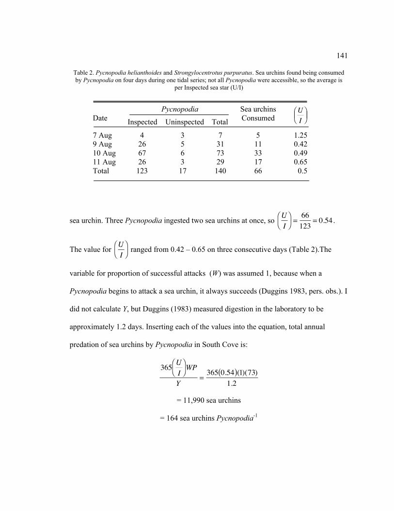
141
Table 2. Pycnopodia helianthoides and Strongylocentrotus purpuratus. Sea urchins found being consumed
by Pycnopodia on four days during one tidal series; not all Pycnopodia were accessible, so the average is
per Inspected sea star (U/I)
Pycnopodia Sea urchins
DateInspected Uninspected Total
Consumed
7 Aug 4 3 7 5 1.25
9 Aug 26 5 31 11 0.42
10 Aug 67 6 73 33 0.49
11 Aug 26 3 29 17 0.65
Total 123 17 140 66 0.5
sea urchin. Three Pycnopodia ingested two sea urchins at once, so
�
U
I
Ê Ë
ˆ ¯
=66
123= 0.54 .
The value for
�
U
I
Ê Ë
ˆ ¯
ranged from 0.42 – 0.65 on three consecutive days (Table 2).The
variable for proportion of successful attacks (W) was assumed 1, because when a
Pycnopodia begins to attack a sea urchin, it always succeeds (Duggins 1983, pers. obs.). I
did not calculate Y, but Duggins (1983) measured digestion in the laboratory to be
approximately 1.2 days. Inserting each of the values into the equation, total annual
predation of sea urchins by Pycnopodia in South Cove is:
�
365U
I
Ê Ë
ˆ ¯ WP
Y=365 0.54( )(1)(73)
1.2
= 11,990 sea urchins
= 164 sea urchins Pycnopodia-1
�
U
I
Ê Ë Á
ˆ ¯ ˜
142
Since 40 Pycnopodia were counted at the East Side and 33 at the West Side, the
respective totals of annual sea urchin predation would be 6570 and 5420 for the study
sites.
Oystercatchers
A flock of five oystercatchers was first observed foraging on sea urchins on the
West Side of South Cove next to tidepools H–K. On another occasion in June, one
oystercatcher was observed eating limpets from the mid-intertidal on the West Side when
the low tide was only 1 m above MLLW. The rest of the observations took place on the
East Side during morning low tides of 0–0.6 m below MLLW, though dead sea urchins
on the West Side provided evidence that oystercatchers occasionally foraged there. I
usually arrived at the study site when the tidal height was above MLLW and falling, and
the oystercatchers often appeared when the tide reached MLLW or shortly thereafter.
Active foraging began once the tidal level dropped to 0.2 m below MLLW and continued
until most or all of the foraging areas were inundated with the rising tide. Data were
collected from 24 February – 11 August, after which the absence of adequate daylight
low tides prevented oystercatchers the opportunity to forage on sea urchins (Fig. 2A).
Since nocturnal foraging has not been described in black oystercatchers, H (annual
number of hours foraging can occur) was set to 127.4, the annual number of daylight
hours that the tidal height was 0.2 m below MLLW (Andres & Falxa 1995).

143
The mean (± SD) number of oystercatchers foraging at low tide was 3.2 ± 1.6 (N
= 28), which was substituted for O in Eq. (3). The maximum number of oystercatchers
observed was five until a sixth was spotted on 28 July. The monthly means are presented
in Fig. 2B. The observed birds may have included one breeding pair, as two
oystercatchers usually foraged together and displayed territorial and mating behavior.
The remaining birds exhibited minimal courtship behavior in May and June, but were
believed to be non-breeding.
0
1
2
3
4
5
Em
erg
en
t d
aylig
ht
ho
urs
B
B
B B
B
B
J F M A M J J A S O N D0
1
2
3
4
5
6
A
B
0.0 m
264 hr
0.6 m
947 hr
-0.2 m
127.4 hr
Fig. 2. Haematopus bachmani. (A) Hours of daylight the tidal level is below 0.6 m, 0.0 m, and –0.2 m
(relative to MLLW); data are pooled per four weeks; (B) the mean (±SE) number of oystercatchers per day
observed foraging on Strongylocentrotus purpuratus between February and August; most accessible S.
purpuratus were below -0.2 m
144
Although sea urchins were present at high densities, oystercatchers continued
walking while foraging, passing by many more sea urchins than they attempted to eat. An
oystercatcher took several steps, touched a sea urchin with its bill, and continued
walking. Multiple sea urchins were tested in this way before the oystercatcher selected
one to eat. When a sea urchin was selected, the oystercatcher braced its legs, wedged its
bill underneath the urchin, and used its bill as a lever to flip the urchin upside-down.
After quickly puncturing the peristomial membrane and usually removing the Aristotle’s
lantern, the oystercatcher inserted its long bill into the urchin and consumed the gonads
without ever breaking the test. The time required to complete each of these activities is
displayed for eight oystercatchers in Fig. 3. The data were collected on five days, but
since no more than six oystercatchers were ever seen at the East Side, a bird may be
represented by more than one trial. The mean (± SD) times required to search for, flip
over, and consume a sea urchin were 54.0 ± 17.3 s, 17.9 ± 12.1 s, and 56.7 ± 14.3 s
respectively. The mean handling time (flipping and consumption) was 74.5 ± 18.7 s.
Summing the three measurements gives 129 seconds (2.15 minutes) for an oystercatcher
to find and eat one sea urchin. This is equivalent to 0.465 urchins min-1
or 28.0 urchins
hour –1
(R).
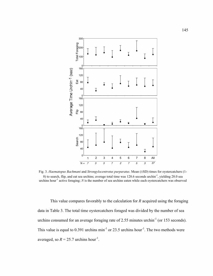
145
J
J
J
J
J
J
J
J
J
1 2 3 4 5 6 7 8 All0
40
80
120
160
Searc
h
J
J
JJ
JJ
J
JJ
0
40
80
120
160
Flip
J
J
J
J
J
JJ
JJ
0
40
80
120
160
Eat
JJ
J
J
J
J
J
J
J
0
100
200
300
Tota
l F
ora
gin
g
N = 7 323 7 573 37
Fig. 3. Haematopus Bachmani and Strongylocentrotus purpuratus. Mean (±SD) times for oystercatchers (1-
8) to search, flip, and eat sea urchins; average total time was 128.6 seconds urchin-1
, yielding 28.0 sea
urchins hour-1
active foraging; N is the number of sea urchins eaten while each oystercatchers was observed
This value compares favorably to the calculation for R acquired using the foraging
data in Table 3. The total time oystercatchers foraged was divided by the number of sea
urchins consumed for an average foraging rate of 2.55 minutes urchin-1
(or 153 seconds).
This value is equal to 0.391 urchins min-1
or 23.5 urchins hour-1
. The two methods were
averaged, so R = 25.7 urchins hour-1
.

146
Table 3. Haematopus bachmani. Time spent foraging and sea urchins consumed by oystercatchers (BLOY)
between February and August 2006; each Continuous Observation is for one oystercatcher, but Time Spent
Foraging is averaged for all oystercatchers present that particular day; all times are in minutes; on three
dates, courtship behavior allowed sex determination, so bold numbers indicate males and underlined
numbers indicate females
Continuous Observations Time Spent Foraging (min)
Date Total BLOY Urchins Time present Time foraging
Foraging Time consumed Min Urchin-1
BLOY-1
day-1
BLOY-1
day-1
24 Feb 4 11 7 1.57 49 42
19 Apr 5
29 Apr 5 9 5 1.8 80 49
30 Apr 3 38 18 2.11 125 125
24 16 1.5
1 May 5 96 52 1.85 130 88
96 21 4.57
12 May 3 8 2 4 26 3
13 May 4
14 May 3 10 4 2.5 60 47
10 9 1.11
15 May 5 25 11 2.27 57 46
25 8 3.13
16 May 3 63 15 4.2 165 165
63 31 2.03
17 May 5 10 4 2.5 136 136
10 4 2.5
26 May 1
27 May 1 131 34 3.85 137 131
28 May 3
12 Jun 1 8 4 2 18 17
14 Jun 5 7 3 2.33 62 60
11 7 1.57
9 3 3
15 Jun 1 22 10 2.67 90 49
16 Jun 5 14 5 2.8 71 41
4 3 1.33
28 Jun 5 47 47
12 Jul 2 29 14 2.33 86 57
18 4 4.5
13 Jul 2
14 Jul 1
24 Jul 3 10 4 2.5 93 76
9 3 3
26 Jul 3
28 Jul 6 57 57
7 Aug 2 37 20
10 Aug 2 11 5 2.2 70 53
11 4 2.7511 Aug 2 10 10
Total 90 792 310 1606 1320
Mean 3.2 28.3 11.1 2.55 Foraging time – 82%
Male 4 175 42 4.17
Female 3 170 90 1.89
147
Of the time oystercatchers were observed, the proportion of time oystercatchers
spent actively foraging (T) was 0.822. Often, upon completing a bout of foraging,
oystercatchers flew to a high rock and preened or loafed. Time spent outside the foraging
area was not included in the calculation for T, unless oystercatchers resumed foraging
after a rest break. Finally, inserting all the parameters into Eq. (3) gives:
(T)(H)(O)(R) = (0.822)(127.4)(3.2)(25.7)
= 8612 sea urchins consumed by oystercatchers
Raccoons
Raccoons were rarely observed eating sea urchins and were extremely wary, so
once they detected humans they quickly left the intertidal for the remainder of that low
tide. The maximum number of raccoons spotted was two, even when they were observed
foraging undisturbed. Most sea urchins preyed upon by raccoons were discovered in the
boulder field, though as the summer progressed, the raccoons seemed to forage with
increasing frequency in the sandy area (see Fig. 1D). The foraging behavior of raccoons
was observed on several occasions. A raccoon selected a sea urchin and grabbed it with
its front paws, sometimes carrying it to a large boulder. The mode of feeding was
dependent on the size of the sea urchin. A relatively small sea urchin (<5.5 cm) was
attacked by biting through the side of the test. A raccoon accessed the insides of a larger
sea urchin by biting chunks of test from the oral side until it could fit its wrist inside the
cavity. The raccoon used its hand to scoop out the gonads and guts, shoveling them
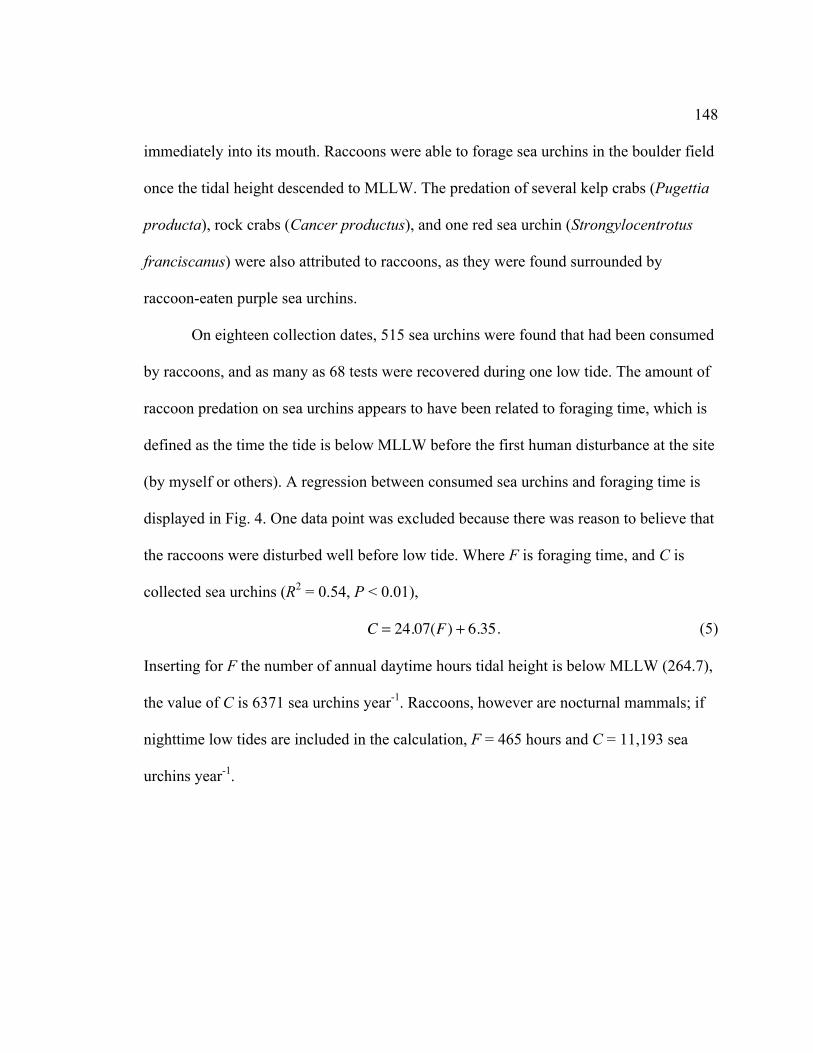
148
immediately into its mouth. Raccoons were able to forage sea urchins in the boulder field
once the tidal height descended to MLLW. The predation of several kelp crabs (Pugettia
producta), rock crabs (Cancer productus), and one red sea urchin (Strongylocentrotus
franciscanus) were also attributed to raccoons, as they were found surrounded by
raccoon-eaten purple sea urchins.
On eighteen collection dates, 515 sea urchins were found that had been consumed
by raccoons, and as many as 68 tests were recovered during one low tide. The amount of
raccoon predation on sea urchins appears to have been related to foraging time, which is
defined as the time the tide is below MLLW before the first human disturbance at the site
(by myself or others). A regression between consumed sea urchins and foraging time is
displayed in Fig. 4. One data point was excluded because there was reason to believe that
the raccoons were disturbed well before low tide. Where F is foraging time, and C is
collected sea urchins (R2 = 0.54, P < 0.01),
�
C = 24.07(F) + 6.35. (5)
Inserting for F the number of annual daytime hours tidal height is below MLLW (264.7),
the value of C is 6371 sea urchins year-1
. Raccoons, however are nocturnal mammals; if
nighttime low tides are included in the calculation, F = 465 hours and C = 11,193 sea
urchins year-1
.
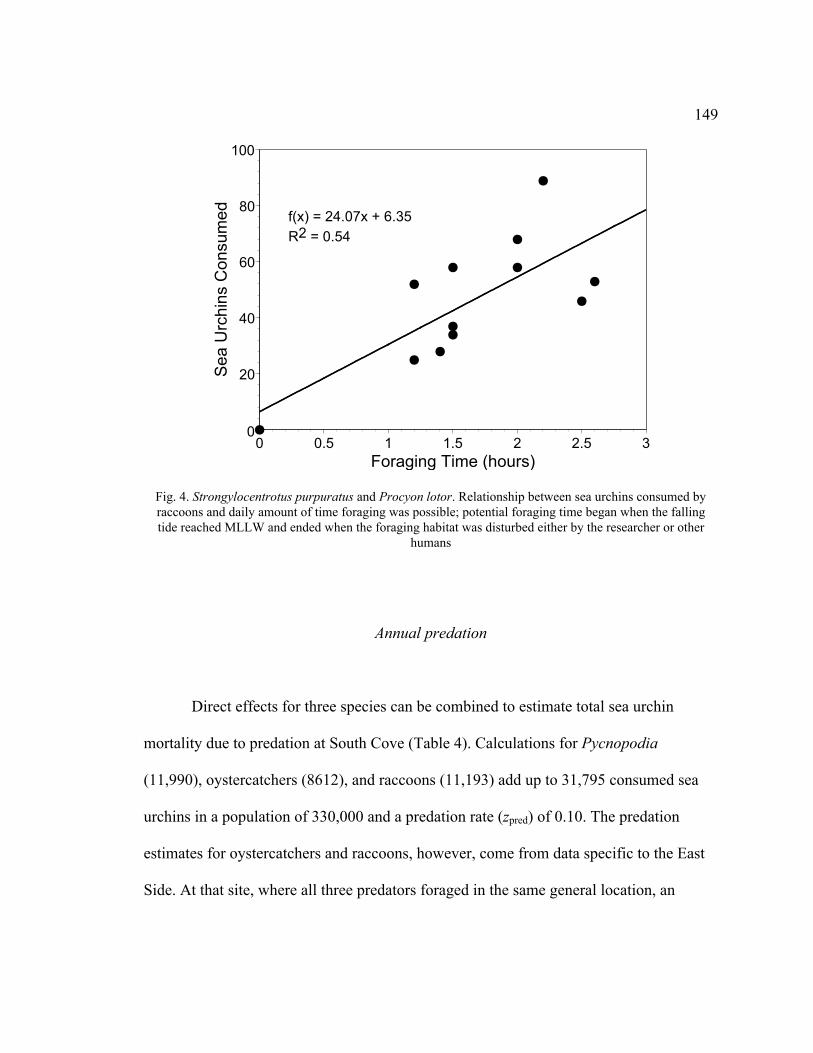
149
J
J
J
J
J
J
J
J
J
J
J
J
0
20
40
60
80
100
0 0.5 1 1.5 2 2.5 3
Se
a U
rch
ins C
on
su
me
d
Foraging Time (hours)
f(x) = 24.07x + 6.35
R2 = 0.54
Fig. 4. Strongylocentrotus purpuratus and Procyon lotor. Relationship between sea urchins consumed by
raccoons and daily amount of time foraging was possible; potential foraging time began when the falling
tide reached MLLW and ended when the foraging habitat was disturbed either by the researcher or other
humans
Annual predation
Direct effects for three species can be combined to estimate total sea urchin
mortality due to predation at South Cove (Table 4). Calculations for Pycnopodia
(11,990), oystercatchers (8612), and raccoons (11,193) add up to 31,795 consumed sea
urchins in a population of 330,000 and a predation rate (zpred) of 0.10. The predation
estimates for oystercatchers and raccoons, however, come from data specific to the East
Side. At that site, where all three predators foraged in the same general location, an
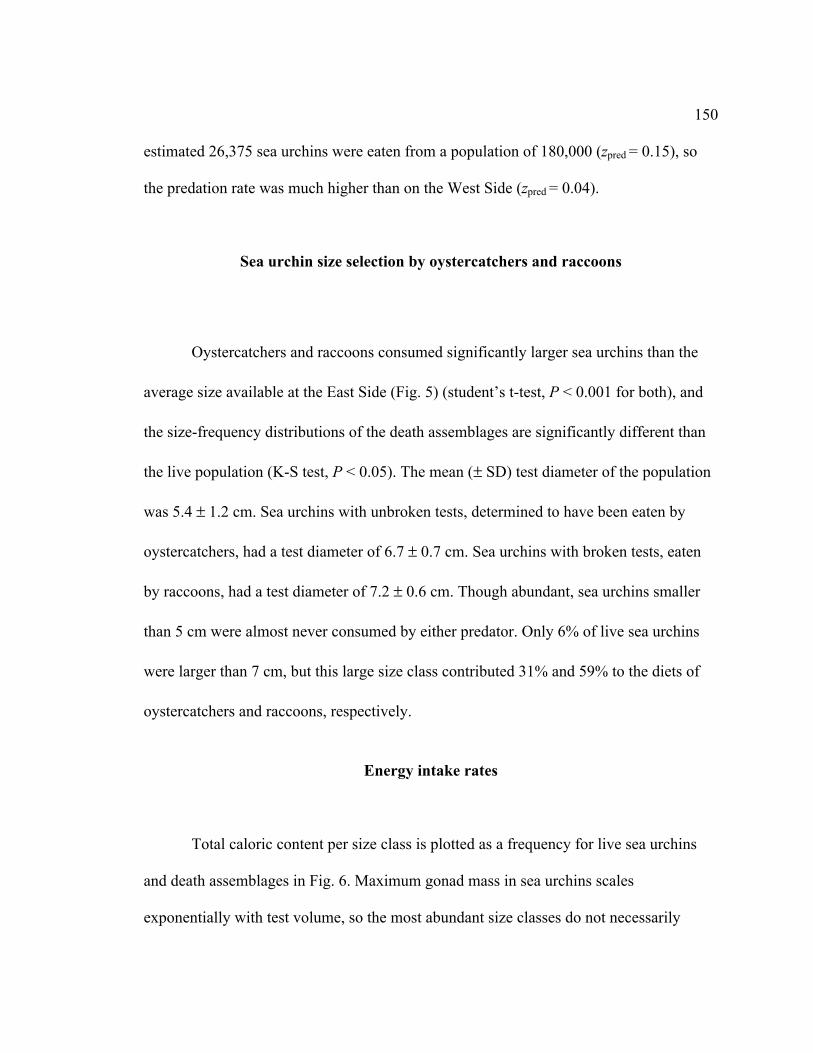
150
estimated 26,375 sea urchins were eaten from a population of 180,000 (zpred = 0.15), so
the predation rate was much higher than on the West Side (zpred = 0.04).
Sea urchin size selection by oystercatchers and raccoons
Oystercatchers and raccoons consumed significantly larger sea urchins than the
average size available at the East Side (Fig. 5) (student’s t-test, P < 0.001 for both), and
the size-frequency distributions of the death assemblages are significantly different than
the live population (K-S test, P < 0.05). The mean (± SD) test diameter of the population
was 5.4 ± 1.2 cm. Sea urchins with unbroken tests, determined to have been eaten by
oystercatchers, had a test diameter of 6.7 ± 0.7 cm. Sea urchins with broken tests, eaten
by raccoons, had a test diameter of 7.2 ± 0.6 cm. Though abundant, sea urchins smaller
than 5 cm were almost never consumed by either predator. Only 6% of live sea urchins
were larger than 7 cm, but this large size class contributed 31% and 59% to the diets of
oystercatchers and raccoons, respectively.
Energy intake rates
Total caloric content per size class is plotted as a frequency for live sea urchins
and death assemblages in Fig. 6. Maximum gonad mass in sea urchins scales
exponentially with test volume, so the most abundant size classes do not necessarily

151
Table 4. Strongylocentrotus purpuratus. Estimates of sea urchin predation by Pycnopodia, oystercatchers,
and raccoons; predation is estimated for each side of South Cove separate and combined; N is the number
of predators for which the estimate is applicable, and U/N is the annual consumption of urchins predator-1
; a
foraging data were not collected on the West Side for oystercatcher and raccoon predation because it was
much less common than on the East Side; b two raccoons were seen on three occasions, and they are
presumed to account for all raccoon predation
Predator West Side East Side Combined N U/N
Pycnopodia 5420 6570 11,990 73 164
Oystercatchersa
8612 8612 3.2 2691
Raccoonsa
11,193 11,193 2b
5547
Total 5420 26,375 31,795
Sea urchins 150,000 180,000 330,000
Predation rate 0.04 0.15 0.10
contain the most calories. A sea urchin with a test diameter equal to the population mean
(5.4 cm) has a caloric content of 15.4 kcal. The average sea urchins consumed by
oystercatchers and raccoons had caloric contents of 27.0 kcal and 33.5 kcal, respectively.
The significance of this size selectivity is that oystercatchers and raccoons consumed a
number of urchins disproportionate to the population. Both predators found and ate sea
urchins over 1 cm larger than the average sized urchin sampled in randomly placed
quadrats. The estimate of 25.7 urchins oystercatcher-1
hour-1
(Fig. 3 and Table 3) can be
multiplied by 27.0 kcal urchin-1
to give an intake rate of 694 kcal oystercatcher-1
hour-1
.
For raccoons, 1 hour is inserted into Eq. (4) as F to give C = 30.4 urchins hour-1
.
Multiplying by an average caloric content of 33.5 kcal urchin-1
gives an intake rate of
1019 kcal raccoon-1
hour-1
.
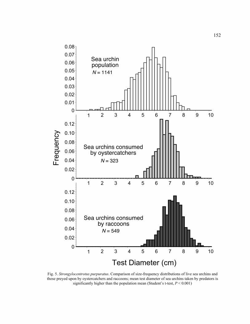
152
1 2 3 4 5 6 7 8 9 100
0.02
0.04
0.06
0.08
0.1
0.12
Test Diameter (cm)
1 2 3 4 5 6 7 8 9 100
0.02
0.04
0.06
0.08
0.1
0.12
Fre
qu
en
cy
Sea urchins consumedby oystercatchers
1 2 3 4 5 6 7 8 9 100
0.01
0.02
0.03
0.04
0.05
0.06
0.07
0.08
Sea urchinpopulation
Sea urchins consumedby raccoons
N = 323
N = 549
N = 1141
0.10
0.10
Fig. 5. Strongylocentrotus purpuratus. Comparison of size-frequency distributions of live sea urchins and
those preyed upon by oystercatchers and raccoons; mean test diameter of sea urchins taken by predators is
significantly higher than the population mean (Student’s t-test, P < 0.001)

Fig. 6. Strongylocentrotus purpuratus. Average caloric content per size class in the sea urchin population and death assemblages; gray bars are the size-
frequency distribution of test diameters; lines are the frequency caloric content in each size class of the sea urchin population (solid line), urchins eaten by
oystercatchers (dotted line), and urchins eaten by raccoons (dotted and dashed line); all data are from the East Side of South Cove
153
1 2 3 4 5 6 7 8 9 100
0.02
0.04
0.06
0.08
0.1
0.12
0.14
0
0.02
0.04
0.06
0.08
0.1
0.12
0.14F
requency
Test Diameter
Sea urchin population
Selected by oystercatchers
Selected by raccoons
Caloric content by size-class

154
DISCUSSION
Observations of abundance and foraging behavior of three predators were used to
estimate the annual rate of predation 32,000 urchins out of 330,000 sea urchins in the
population. On the East Side, where all three predators forage, about 26,000 of 180,000
sea urchins were predicted to be eaten, a predation rate of nearly 15%. Although South
Cove’s intertidal is teeming with sea urchins, if the predation rates observed in 2006
continue several years, the ramifications for the population could be significant.
Considering the variable nature of sea urchin recruitment in Oregon (Ebert 1968, Ebert &
Russell 1988), sea urchin abundance in South Cove could decrease by 50% in less than a
decade due to predation pressure alone. I did not observe any major pulses of sea urchin
recruitment in 2005 or 2006 to counteract the high mortality rate.
Pycnopodia density and predation
Pycnopodia are generalist predators that have been observed to specialize on
purple sea urchins in Alaska (Duggins 1983), Washington (Mauzey et al. 1968, Dayton
1975), and California (Tegner & Dayton 1981), but they are not an obligate diet item
(Mauzey et al. 1968, Herrlinger 1983). Pycnopodia are abundant at South Cove, often
occurring in tidepools and underneath boulders or seaweed. However, the densities
observed in tidepools in February 2006 (0.9–2.6 Pycnopodia m-2
) were uncommonly
high. Dayton (1973), who was the first to describe urchin stampeding, said that such

155
densities were an order of magnitude higher than what he has observed (personal
communication). No published densities that I am aware of approach the 2.6 sea stars m-2
recorded in one tidepool. Densities reported in subtidal surveys in California,
Washington, and Alaska range from 0.01 to 0.1 Pycnopodia m-2 (Wobber 1975, Duggins
1981, Watanabe 1984, Kvitek et al. 1992), and Wootton (1997) reported 0.09 Pycnopodia
m-1
shoreline in Washington. In South Cove, 73 Pycnopodia were counted along
approximately a 300 m shoreline (0.24 Pycnopodia m-1
total shoreline, 0.34 Pycnopodia
m-1
East Side shoreline).
Unfortunately, little can be said about the temporal change in Pycnopodia density
because of the lack of data, which were collected sporadically during eight months in
2006. I did not visit South Cove after August 2005 until January 2006, when the
observations described in this paper began, so I can only speculate as to the events
preceding the urchin stampedes. It seems that for some reason, Pycnopodia were driven
to aggregate in large tidepools during the fall of 2005 or early winter of 2006. It is
possible, but highly unlikely, that the Pycnopodia were in the tidepools in the summer of
2005 and escaped notice. For one, the bright colors and large size (ca. 0.4–0.6 m
diameter) of Pycnopodia made them easily visible. Second, the urchin stampedes
appeared to have occurred recently because no organisms had colonized their former
scars, circular patches of bare rock surrounded by coralline algae.
What might have caused dozens of large, highly mobile predators to invade the
tidepools? Perhaps changes in the physical environment or in subtidal prey populations
led to high intertidal predator densities. In Oregon, water temperature can alter the

156
foraging behavior of the sea star Pisaster ochraceus (Sanford 2002b). During summer
periods of upwelling, when water temperature dropped from 12° to 8°C, intertidal sea star
density decreased as individuals moved into surge channels and the shallow subtidal.
Warmer ocean temperatures in the winter could explain increased foraging activity by
Pycnopodia, but sea surface temperatures were not particularly warm in January 2006.
Pycnopodia has been shown to prefer the bivalve Saxidomus giganteus (Mauzey et al.
1968) to Strongylocentrotus purpuratus, and subtidal seastar populations often feed
primarily on mollusks, even when sea urchins are present (Mauzey et al. 1968, Herrlinger
1983, Shivji et al. 1983). A die-off of a subtidal prey species such as S. giganteus might
have prompted Pycnopodia to utilize intertidal sea urchins as a secondary food source.
Regardless of the reason that high intertidal densities of Pycnopodia occurred in
early 2006, once there, the effects on purple sea urchins were considerable. The per
capita consumption estimate of 164 urchins year-1
is much higher than that for a subtidal
population in Torch Bay, Alaska, where individual Pycnopodia were estimated to eat 44
urchins year-1
(Duggins 1983). The frequency of Pycnopodia consuming sea urchins was
19% in Alaska but over 50% in South Cove, suggesting higher intake rates are partially
responsible for larger estimates of predation. In this study, Pycnopodia also displayed
greater preference for sea urchins than in Alaska, where one-third of feeding sea starts
were consuming prey items other than sea urchins (Duggins 1983).
My determination of predation by Pycnopodia should be treated as tentative.
First, it is problematic that predation events were enumerated only in August, because
temporal variability in predation rates or prey selection would affect the estimated direct

157
effects calculated for a whole year. Second, temperature has been shown to affect feeding
in asteroids, and warmer temperatures are usually associated with higher metabolic and
foraging activity (Sloan 1980, Sanford 2002a). Since average seawater temperature is
higher in Oregon than Alaska, Pycnopodia could have higher metabolic rates and
consume more sea urchins. Duggins’ (1983) calculated digestion time, 1.2 days, maybe
longer than the digestion time for Pycnopodia in Oregon, suggesting that 164 urchins
year-1
could be an underestimate.
Indirect effects due to Pycnopodia
Pycnopodia’s direct effects on sea urchins appeared to be substantial, but its
indirect effects were even more pronounced. Dayton (1975) found that the emigration
rate of sea urchins in stampedes was eight to twelve times higher than one sea star’s
consumption rate. I observed similarly large numbers of sea urchins stampeding from
tidepools, but the risk of wave dislodgement was less than for Dayton’s exposed
populations, so green sea anemones were not privy to easy meals. Instead, at South Cove,
trait-mediated behavior in sea urchins benefited oystercatchers and raccoons.
Oystercatchers easily flipped sea urchins that had moved to tenuous locations on the tops
of rocks and other urchins. The presence of Pycnopodia also caused many sea urchins to
abandon the relative safety of their pits or the tidepool. I never observed an oystercatcher
pry a sea urchin out of its pit, though one occasionally would test a pit urchin with its bill
before moving on to easier targets. Even a sea urchin outside of a pit cannot be eaten by
158
an oystercatcher if it is underwater; it was rare for an oystercatcher to put its face into the
water to prey on an urchin. By chasing sea urchins out of tidepools, Pycnopodia caused
them to be more accessible and exposed for a longer time at low tide, increasing the
foraging capabilities of oystercatchers.
Urchin stampedes were most prevalent next to the boulder field where raccoons
tended to forage. During the summer, there were consistently 15–25 Pycnopodia in the
shallow surge channel adjacent to the boulder field. Like oystercatchers, raccoons
indirectly benefited from the Pycnopodia chasing sea urchins out of the water. Many of
the sea urchins in the boulder field stampeded out of subtidal surge channels that would
have been more difficult for raccoons to access.
The ability to detect waterborne chemical cues allows sea urchins to flee a marine
predator, but does nothing to help them avoid terrestrial predators. Annual estimated
predation on the East Side is over 26,000 sea urchins, of which Pycnopodia only
consumed 6500. The other 19,500 sea urchins were eaten by terrestrial predators that
forage at low tide when sea urchins are unable to move or use chemosensory capabilities.
The irony here is that by reacting to the presence of Pycnopodia, purple sea urchins were
more likely to suffer mortality than if they had remained sedentary. Pycnopodia’s indirect
effects led to more predation events than actual consumption.
Oystercatchers and raccoons benefited from Pycnopodia’s indirect effects on sea
urchins, and they had their own positive indirect effects on other species. An interaction
web displays this suite of interactions between sea urchins, predators, and scavengers at
South Cove (Fig. 7). American crows (Corvus brachyrhynchos) were often seen
159
scavenging moribund sea urchins after raccoons or oystercatchers moved away. Larus
occidentalis, the western gull, was often present at South Cove and sometimes
approached foraging oystercatchers. Kleptoparasitism was observed on several occasions,
and usually consisted of a gull swallowing the discarded Aristotle’s lantern. Neither gulls
nor crows were observed to prey on live sea urchins at South Cove, though I often saw
them near the West Side urchin stampedes. Gulls and crows have been observed to prey
on sea urchins and they certainly had the opportunity to do so at South Cove (Irons et al.
1986, Wootton 1995, 1997, Snellen 2006). Another positive indirect effect of
oystercatchers and raccoons exists for green sea anemones, many of which were
discovered digesting sea urchins that were preyed upon by raccoons. Since South Cove is
a protected site, these sit-and-wait predators did not benefit from Pycnopodia chasing sea
urchins into positions where waves would dislodge them. Instead, during low tides, the
activity of terrestrial predators created a stock of dead sea urchins that were washed
around when the tide rose.
Trait-mediated indirect effects have been demonstrated in many ecosystems, and
they are often stronger than direct effects (reviewed in Preisser et al. 2005). This seems to
be the case at South Cove, and the species interactions described do not even consider the
indirect effects of removing thousands of invertebrate grazers and space-holders from the
intertidal. This complex web of community interactions was set into motion because of a
change in density of one species, Pycnopodia. Multi-trophic studies that do not consider
indirect effects could severely misestimate community dynamics, just as I would have
underestimated Pycnopodia’s effects if I had ignored its indirect effects.
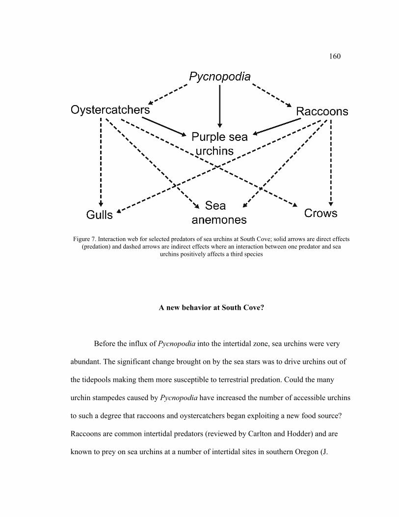
160
Figure 7. Interaction web for selected predators of sea urchins at South Cove; solid arrows are direct effects
(predation) and dashed arrows are indirect effects where an interaction between one predator and sea
urchins positively affects a third species
A new behavior at South Cove?
Before the influx of Pycnopodia into the intertidal zone, sea urchins were very
abundant. The significant change brought on by the sea stars was to drive urchins out of
the tidepools making them more susceptible to terrestrial predation. Could the many
urchin stampedes caused by Pycnopodia have increased the number of accessible urchins
to such a degree that raccoons and oystercatchers began exploiting a new food source?
Raccoons are common intertidal predators (reviewed by Carlton and Hodder) and are
known to prey on sea urchins at a number of intertidal sites in southern Oregon (J.

161
Hodder, personal communication). Broken tests were observed at South Cove in August
2005, indicating that raccoons were foraging on sea urchins before Pycnopodia increased
in density.
Oystercatchers, too, have previously been observed to eat sea urchins (Falxa
1992, Wootton 1997), but it is unknown whether they have exhibited this behavior at
South Cove. A clue that they have is the expediency they showed in taking advantage of
the food source. Sea urchins are exposed for few daylight hours in the winter, and by
February, oystercatchers were already foraging during those narrow windows of
opportunity. Deft bill work is required to flip a sea urchin and eat its gonads, technical
enough that these oystercatchers probably had prior experience eating sea urchins (Falxa
1992).
Alternatively, the death assemblage data suggest oystercatchers and raccoons may
be in the initial stages of profiting from a glut of food. Kvitek et al. (1992) present sea
urchin size frequency data from areas inhabited by sea otters. Sea otters prey heavily on
sea urchins and within a short time can eliminate the largest size classes in an area.
Despite the selection of large urchins by oystercatchers and raccoons, the population
structure at South Cove still contains many large individuals, thought the mean test
diameter of sea urchins outside pits did decrease by about 0.5 cm between 2005 and 2006
(see Chapter II). The hypothesis that oystercatchers and raccoons have only recently been
focusing their foraging efforts on sea urchins, would be supported if sea urchin size
continues to show annual decreases.
162
Optimal foraging behavior
Oystercatchers are known for specialization in prey type and foraging behavior.
Most of the research on this topic has focused on Haematopus ostralegus, the European
oystercatcher, while the black oystercatcher of the North American Pacific coast is better
described as a generalist that is capable of exploiting a variety of food sources including
limpets, mussels, worms, and sea urchins (Hartwick 1978, Frank 1982, Falxa 1992,
Wootton 1997).
In several studies, Oystercatchers have been observed to exhibit optimal foraging
behavior (Hartwick 1976, Zwarts & Wanink 1984, Meire & Ervynck 1986, Cayford &
Goss-Custard 1990)}. Again, most literature focuses on the European oystercatcher, and
my observations provide evidence that black oystercatchers are also optimal foragers.
The central premise of the theory of optimality is that an organism forages on the prey
type that provides the most energy per searching and handling time (Krebs & Davies
1993). My lack of size-specific searching and handling times prevents the application of
an optimality model. However, by selecting sizes of sea urchins larger than what is
commonly available on the East Side, both oystercatchers and raccoons seem to be
choosing the most optimal prey.
Gonad production in purple sea urchins is cyclic (Boolootian 1966). Gonad index
[(gonad mass) (body mass-1
)] increases during the growing season when food is plentiful
until it peaks at 15–25% in December or January when spawning occurs. Coincidentally,
gonad index is smallest in March and April, soon after oystercatchers began feeding on
163
sea urchins. (Due to this temporal variability associated with gonad indices, following
calculations should be considered nothing more than rough estimates.) At South Cove,
the gonad index in May 2006 was only 3.5%, down from 7.4% in February and 11.0% in
August 2005 (unpublished data). Based on these measurements and Boolootian’s (1966)
ten-year dataset of monthly gonad indices, 7.5% is a reasonable estimation for gonad
index between April and August, when most oystercatchers were observed foraging. My
calculations of caloric content were based on data collected sometime between
September and March (Snellen 2006), when the gonad index was probably about twice
this value (Boolootian 1966, Gonor 1972). So therefore, if I decrease my caloric content
calculations by half, oystercatchers are estimated to consume 13.5 instead of 27 kcal
urchin-1
and 347 instead of 693 kcal hour-1
. Black oystercatchers are approximately the
same size as their European counterparts (Swennen 1984, Andres & Falxa 1995), so they
presumably have similar basal metabolic rates (BMR). BMR is 251 kJ day-1
, or 60 kcal
day-1
, for a European oystercatcher (Kersten & Piersma 1987). Food intake rates are
about 3.2 times the BMR, so 187 kcal must be ingested daily to maintain weight (Goss-
Custard 1996). Given an average caloric content of 13.5 kcal urchin-1
, an adult
oystercatcher would need to consume fourteen sea urchins to fulfill its daily energy
requirement. In April and May, when gonad indices may be less than 4%, an
oystercatcher might require 28 sea urchins to meet its energy needs, but much less
foraging would be necessary in the fall or winter when gonad index is higher. These
calculations suggest that at South Cove, black oystercatchers can consume enough sea
164
urchins during one low tide to meet their daily energy requirement, assuming the water
level is at least 0.2 m below MLLW.
Based on field observations of oystercatchers, I calculated a foraging rate of 25.7
urchins hour–1
, which seems excessive considering their estimated energetic needs. The
possibility exists that European and black oystercatchers actually vary in their BMR, and
I erred in assuming them equal. A second explanation for the high foraging rates is a bias
toward field observations early in the summer (mid-April to mid-June) compared to late
(mid-June to mid-August). Females lay their eggs in late May (Andres & Falxa 1995),
and the additional energy required for this task could in much higher foraging rates than
males (Ricklefs 1974 in Ross 1979). I was only able to distinguish between male and
female birds on three days, but the data clearly showed much higher foraging rates in
female oystercatchers (Table 3). My seemingly high estimates of energy intake are likely
be the result of foraging by females preparing to lay eggs.
Since black oystercatchers, unlike European oystercatchers, do not forage at night
(Andres & Falxa 1995), they cannot take utilize intertidal sea urchins as a food source in
the winter when gonad indices peak. Raccoons, however, are nocturnal foragers and may
be able to exploit the sea urchin population at South Cove year round. Winter foraging
would be even more rewarding for raccoons than oystercatchers since they tend to prey
on larger sea urchins (Fig. 6). The foraging behaviors of these terrestrial predators,
facilitated by a marine predator, place a disproportionate pressure on the largest size
classes of purple sea urchins. This complex web of indirect effects demonstrates the

165
potential for energy flow between habitats and has implications for trophic dynamics in
other coastal ecosystems.
166
CHAPTER VI
CONCLUDING SUMMARY
The chapters contained in this thesis stand alone, but they are also puzzle pieces
that can be fit together to address a larger question: what are the effects of differential
microhabitat use in Strongylocentrotus purpuratus? Chapter II highlights the differences
between sea urchins living inside and outside pits. Morphologically speaking, pit
microhabitats result in sea urchins with shorter spines, larger jaws, and different test
shapes relative to those in nonpit microhabitats. Additionally, the size structure of sea
urchins is affected by microhabitat, as nonpit urchins are consistently larger than pit
urchins. The remaining thesis chapters relate to three hypotheses addressing this
difference in size: differential growth (Chapter III), movement out of pits (Chapter IV),
and differential mortality (Chapter V).
Chapter III focuses on microhabitat-specific growth rates, which were higher in
sea urchins living outside pits than inside pits. Faster growth and smaller relative jaw size
(Chapter II) are clues that nonpit urchins receive more food than pit urchins. However,
despite faster growth, age-frequency distributions created from the growth curves
indicate that the nonpit urchins were older, and thus, had been growing longer, than the
pit urchins. If pit and nonpit urchins were permanently sedentary, there would be a
smaller gap in size difference than what was observed. An alternative explanation for the

167
large difference in mean diameters is that pit urchins move out of their pits once they
grow to a certain size.
In Chapter IV, I investigated movement in purple sea urchins primarily by
monitoring marked plots in tidepools at South Cove. Over the course of one year, I found
that movement was quite rare in this intertidal population of sea urchins. In fact, at the
end of the monitoring period, 94% of the sea urchins remaining had been sedentary as
long as I had been observing them. Movement in Strongylocentrotus purpuratus seems to
be very infrequent; this result was not unexpected, considering observations by other
scientists and the morphological differences between pit and nonpit urchins. The
movement detected, though rare, probably contributes to the larger size of nonpit urchins
along with differential growth rates.
If pit urchins are smaller than nonpit urchins, it could also simply be a result of
higher mortality. However, as I describe in Chapter V, the major source of mortality,
predation, acted selectively on nonpit urchins. At South Cove, in the winter of 2005 –
2006, the intertidal population of the sea star Pycnopodia helianthoides exploded, and I
observed densities that were orders of magnitude higher than normal. Since purple sea
urchins are a common prey item of Pycnopodia, they stampeded from dozens of tidepools
creating huge piles of sea urchins. It was not long before terrestrial predators began
exploiting this food resource, and I observed a handful of oystercatchers and raccoons
feeding on thousands of sea urchins throughout the spring and summer of 2006. These
results are presented in light of trait-mediated indirect effects and optimal foraging
behavior, but they also address the overall question of the effects of microhabitat on sea
168
urchins. Predation of pit urchins was never observed, and it is possible that pits reduce
rather than enhance mortality.
These chapters combine to tell a story of trade-offs between microhabitats. A sea
urchin may have higher survivorship as long as it remains inside a pit. The negative
trade-off of this sedentary lifestyle could be food limitation, constrained outward growth,
or both, which result in smaller size than nonpit urchins. A slightly higher growth rate
over several decades yields a significant difference in volume, and therefore, maximum
reproductive output, which might be two-to-three times greater in a nonpit urchin than a
pit urchin of the same age. So, is it preferable to risk death and grow to a large size
quickly to release more gametes, or would an urchin be “wise” to remain in its pit and
make a smaller contribution to (presumably) more reproductive events. The lack of
movement evident at South Cove indicates that different sea urchins probably utilize both
strategies; one can certainly find areas in which sea urchins occupy only one of these two
microhabitats because there is no choice to be had.
The value of this research increases when one thinks outside of the world of sea
urchins and considers the other invertebrates to which these findings might apply. All
habitats contain various microhabitats, the most desirable of which are often selected by
mobile organisms. It might be more important to consider the microhabitat of sessile and
sedentary invertebrates that cannot easily escape their present physical environment. As
exampled by sea urchins, these organisms could experience a high degree of
microhabitat-based effects influencing growth, reproduction, and other biological and
ecological factors.
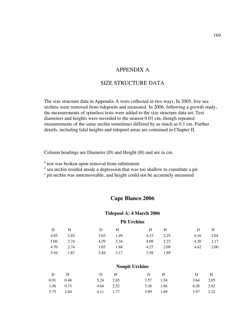
169
APPENDIX A
SIZE STRUCTURE DATA
The size structure data in Appendix A were collected in two ways. In 2005, live sea
urchins were removed from tidepools and measured. In 2006, following a growth study,
the measurements of spineless tests were added to the size structure data set. Test
diameters and heights were recorded to the nearest 0.01 cm, though repeated
measurements of the same urchin sometimes differed by as much as 0.1 cm. Further
details, including tidal heights and tidepool areas are contained in Chapter II.
Column headings are Diameter (D) and Height (H) and are in cm.
b test was broken upon removal from substratumd sea urchin resided inside a depression that was too shallow to constitute a pitu pit urchin was unremoveable, and height could not be accurately measured
Cape Blanco 2006
Tidepool A: 4 March 2006
Pit Urchins
D H D H D H D H
4.85 2.82
5.06 2.74
4.70 2.74
3.94 1.87
3.03 1.49
4.59 2.34
3.05 1.68
5.84 3.17
4.33 2.25
4.09 2.23
4.27 2.09
3.58 1.89
4.16 2.04
4.20 2.17
4.42 2.00
Nonpit Urchins
D H D H D H D H
0.91 0.48
1.56 0.73
5.75 2.84
5.24 2.65
4.64 2.52
4.11 1.77
3.57 1.54
3.36 1.66
3.99 1.69
3.64 2.05
4.28 2.02
3.97 2.22

Cape Blanco 2006 170
D H D H D H D H
5.02 2.28
4.59 2.46
4.19 2.14
5.60 2.86
3.73 1.80
4.88 2.30
5.33 2.73
4.03 1.66
4.52 2.35
4.62 2.38
4.90 2.50
5.22 2.69
5.04 2.54
4.83 1.98
4.80 2.31
5.36 2.81
4.90 2.22
Tidepool B: 4 March 2006
Pit Urchins
D H D H D H D H
3.96 2.35
3.79 2.09
3.13
3.94
3.90
3.34
1.44 0.70
3.97 2.26
3.51 1.82
3.48 2.18
3.75 2.03
4.27 2.35
4.33 2.12
3.90 2.39
3.33 1.79
3.74 1.80
4.03 1.93
3.10 1.63
3.83 1.95
4.18 2.25
3.88 2.16
2.35 1.03
2.24 1.25
3.33 1.75
2.69 1.20
4.72 2.36
5.72 3.05
5.17 3.12
4.64 2.53
5.99 3.62
Nonpit Urchins
D H D H D H D H
0.50 0.22
6.08 2.76
6.21 2.89
6.16 2.94
5.44 2.44
5.91 2.78
4.64 1.98
3.36 1.24
4.45 2.11
5.19 2.39
6.58 3.16
5.69 2.77
5.36 2.66
4.94 2.12
5.82 2.58
6.24 2.91
4.66 2.24
4.32 2.13
4.83 2.01
6.78 2.72
5.42 2.64
6.04 2.73
6.13 2.84
5.76 3.10
5.64 2.65
6.13 3.00
6.27 3.09
5.60 2.30
4.73 2.37
4.53 2.02
5.33 2.36
5.70 2.97
5.81 2.67
5.26 2.33
4.48 1.78
5.40 2.71
5.89 2.99
6.10 3.08
5.20 2.73
4.38 2.01
4.31 2.00
4.54 2.34
6.26 2.96
6.95 3.31
6.73 3.03
3.40 1.59
5.11 2.24
4.20 2.02
3.35 1.34
3.96 1.98
6.56 3.33
5.10 2.38
6.49 3.12
5.46 2.81
5.34 2.55
4.18 2.21
5.61 2.62
5.27 2.24
5.75 3.18
4.43 2.35
4.09 1.98
4.69 2.27
4.86 2.15
6.40 3.34
6.27 2.52
4.26 1.85
5.64 2.39
5.22 2.48
4.69 2.02
7.28 3.65
4.42 2.44
5.56 2.86
6.56 3.19
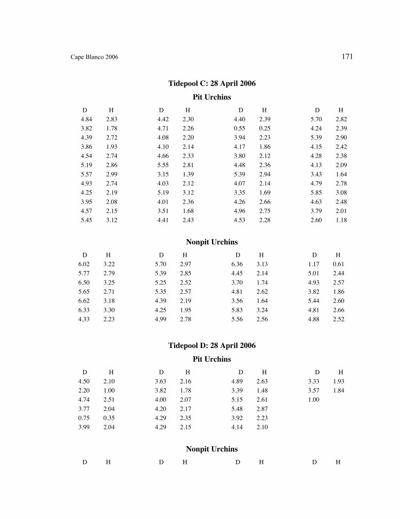
Cape Blanco 2006 171
Tidepool C: 28 April 2006
Pit Urchins
D H D H D H D H
4.84 2.83
3.82 1.78
4.39 2.72
3.86 1.93
4.54 2.74
5.19 2.86
5.57 2.99
4.93 2.74
4.25 2.19
3.95 2.08
4.57 2.15
5.45 3.12
4.42 2.30
4.71 2.26
4.08 2.20
4.10 2.14
4.66 2.33
5.55 2.81
3.15 1.39
4.03 2.12
5.19 3.12
4.01 2.36
3.51 1.68
4.41 2.43
4.40 2.39
0.55 0.25
3.94 2.23
4.17 1.86
3.80 2.12
4.48 2.36
5.39 2.94
4.07 2.14
3.35 1.69
4.26 2.66
4.96 2.75
4.53 2.28
5.70 2.82
4.24 2.39
5.39 2.90
4.15 2.42
4.28 2.38
4.13 2.09
3.43 1.64
4.79 2.78
5.85 3.08
4.63 2.48
3.79 2.01
2.60 1.18
Nonpit Urchins
D H D H D H D H
6.02 3.22
5.77 2.79
6.50 3.25
5.65 2.71
6.62 3.18
6.33 3.30
4.33 2.23
5.70 2.97
5.39 2.85
5.25 2.52
5.35 2.57
4.39 2.19
4.25 1.95
4.99 2.78
6.36 3.13
4.45 2.14
3.70 1.74
4.81 2.62
3.56 1.64
5.83 3.24
5.56 2.56
1.17 0.61
5.01 2.44
4.93 2.57
3.82 1.86
5.44 2.60
4.81 2.66
4.88 2.52
Tidepool D: 28 April 2006
Pit Urchins
D H D H D H D H
4.50 2.10
2.20 1.00
4.74 2.51
3.77 2.04
0.75 0.35
3.99 2.04
3.63 2.16
3.82 1.78
4.00 2.07
4.20 2.17
4.29 2.35
4.29 2.15
4.89 2.63
3.39 1.48
5.15 2.61
5.48 2.87
3.92 2.23
4.14 2.10
3.33 1.93
3.57 1.84
1.00
Nonpit Urchins
D H D H D H D H
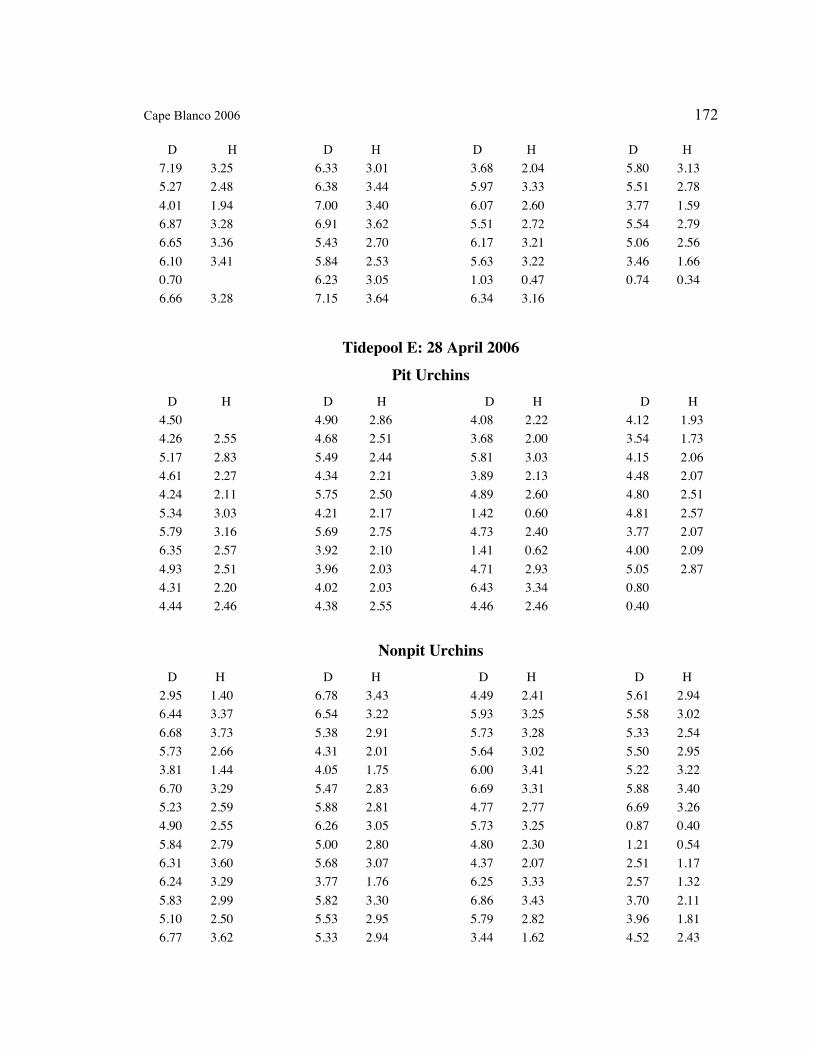
Cape Blanco 2006 172
D H D H D H D H
7.19 3.25
5.27 2.48
4.01 1.94
6.87 3.28
6.65 3.36
6.10 3.41
0.70
6.66 3.28
6.33 3.01
6.38 3.44
7.00 3.40
6.91 3.62
5.43 2.70
5.84 2.53
6.23 3.05
7.15 3.64
3.68 2.04
5.97 3.33
6.07 2.60
5.51 2.72
6.17 3.21
5.63 3.22
1.03 0.47
6.34 3.16
5.80 3.13
5.51 2.78
3.77 1.59
5.54 2.79
5.06 2.56
3.46 1.66
0.74 0.34
Tidepool E: 28 April 2006
Pit Urchins
D H D H D H D H
4.50
4.26 2.55
5.17 2.83
4.61 2.27
4.24 2.11
5.34 3.03
5.79 3.16
6.35 2.57
4.93 2.51
4.31 2.20
4.44 2.46
4.90 2.86
4.68 2.51
5.49 2.44
4.34 2.21
5.75 2.50
4.21 2.17
5.69 2.75
3.92 2.10
3.96 2.03
4.02 2.03
4.38 2.55
4.08 2.22
3.68 2.00
5.81 3.03
3.89 2.13
4.89 2.60
1.42 0.60
4.73 2.40
1.41 0.62
4.71 2.93
6.43 3.34
4.46 2.46
4.12 1.93
3.54 1.73
4.15 2.06
4.48 2.07
4.80 2.51
4.81 2.57
3.77 2.07
4.00 2.09
5.05 2.87
0.80
0.40
Nonpit Urchins
D H D H D H D H
2.95 1.40
6.44 3.37
6.68 3.73
5.73 2.66
3.81 1.44
6.70 3.29
5.23 2.59
4.90 2.55
5.84 2.79
6.31 3.60
6.24 3.29
5.83 2.99
5.10 2.50
6.77 3.62
6.78 3.43
6.54 3.22
5.38 2.91
4.31 2.01
4.05 1.75
5.47 2.83
5.88 2.81
6.26 3.05
5.00 2.80
5.68 3.07
3.77 1.76
5.82 3.30
5.53 2.95
5.33 2.94
4.49 2.41
5.93 3.25
5.73 3.28
5.64 3.02
6.00 3.41
6.69 3.31
4.77 2.77
5.73 3.25
4.80 2.30
4.37 2.07
6.25 3.33
6.86 3.43
5.79 2.82
3.44 1.62
5.61 2.94
5.58 3.02
5.33 2.54
5.50 2.95
5.22 3.22
5.88 3.40
6.69 3.26
0.87 0.40
1.21 0.54
2.51 1.17
2.57 1.32
3.70 2.11
3.96 1.81
4.52 2.43

Cape Blanco 2006 173
D H D H D H D H
4.66 2.19
5.06 2.99
5.22 2.78
4.87 2.22
5.55 2.90
5.38 3.10
5.91 3.32
6.37 3.23
5.97 3.26
0.55 0.22
Cape Blanco 2005
Tidepool F: 26 April 2005
Pit Urchins
D H D H D H D H
1.59 0.68
2.07 1.02
2.59 1.29
2.66 1.22
2.85 1.74 b
2.96 1.51
3.10 1.68
3.18 1.72 b
3.18 2.14
3.47 1.78
3.56 1.91
3.57 2.04 b
3.64 1.62
3.72 1.75
3.89 1.87
3.89 2.43
3.97 2.32 b
4.04 2.05
4.08 2.18
4.16 1.96 b
4.24 2.22
4.29 2.34
4.34 2.10
4.93 2.65
5.13 2.54
Nonpit Urchins
D H D H D H D H
1.39 0.57
2.25 0.95
2.50 1.07
4.24 2.11
4.48 2.12 d
4.60 2.37
4.68 2.04
4.81 2.60
5.01 3.09 d
5.06 2.49
5.10 2.67 d
5.19 2.36
5.21 2.58 d
5.31 2.30
5.32 2.41
5.33 2.39
5.44 2.55
5.63 2.77
5.63 2.63
5.84 2.96
5.87 2.77
5.88 3.06
5.92 3.04
5.94 2.69
5.97 3.27
6.10 3.07
6.17 2.89
6.34 3.18
6.58 3.06
Tidepool G: 29 April 2005
Pit Urchins
D H D H D H D H
2.37 1.15
3.26 1.74
3.20 1.64
3.03 1.65
3.68 u
3.75 u
4.79 u
2.89 1.55
3.48 u
2.54 1.20
2.69 u
2.98 u
2.58
3.09 1.71
3.36 1.71
2.92 u
2.22 u
3.79 u
3.72 u
2.71 1.60
3.07 1.62
3.68 2.11
3.04 1.65
2.25 1.20
4.79 u
3.46 u
3.51 1.89
2.72 u
4.54 u
3.84 u
3.72 u
3.54 1.97
4.03 2.20
3.71 1.72
4.23 2.42
4.77 u
3.47 u
4.42 u
4.59 2.61
5.35 2.78
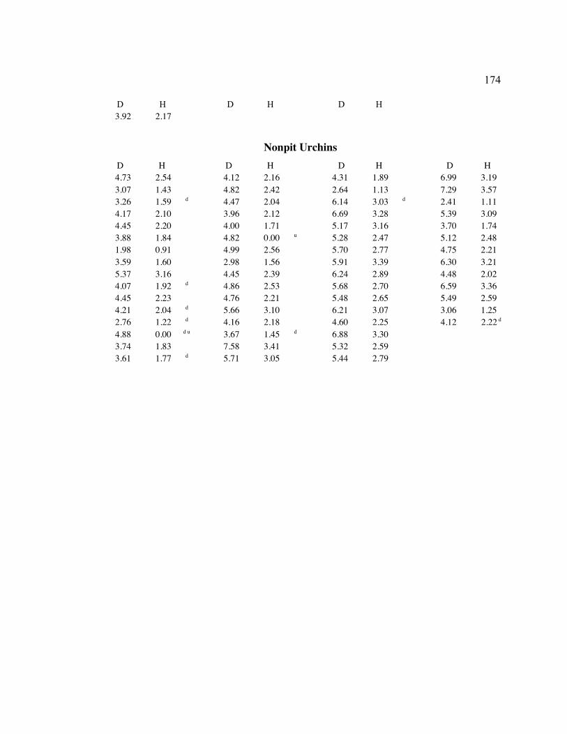
174
D H D H D H
3.92 2.17
Nonpit Urchins
D H D H D H D H
4.73 2.54
3.07 1.43
3.26 1.59 d
4.17 2.10
4.45 2.20
3.88 1.84
1.98 0.91
3.59 1.60
5.37 3.16
4.07 1.92 d
4.45 2.23
4.21 2.04 d
2.76 1.22 d
4.88 0.00 d u
3.74 1.83
3.61 1.77 d
4.12 2.16
4.82 2.42
4.47 2.04
3.96 2.12
4.00 1.71
4.82 0.00 u
4.99 2.56
2.98 1.56
4.45 2.39
4.86 2.53
4.76 2.21
5.66 3.10
4.16 2.18
3.67 1.45 d
7.58 3.41
5.71 3.05
4.31 1.89
2.64 1.13
6.14 3.03 d
6.69 3.28
5.17 3.16
5.28 2.47
5.70 2.77
5.91 3.39
6.24 2.89
5.68 2.70
5.48 2.65
6.21 3.07
4.60 2.25
6.88 3.30
5.32 2.59
5.44 2.79
6.99 3.19
7.29 3.57
2.41 1.11
5.39 3.09
3.70 1.74
5.12 2.48
4.75 2.21
6.30 3.21
4.48 2.02
6.59 3.36
5.49 2.59
3.06 1.25
4.12 2.22 d
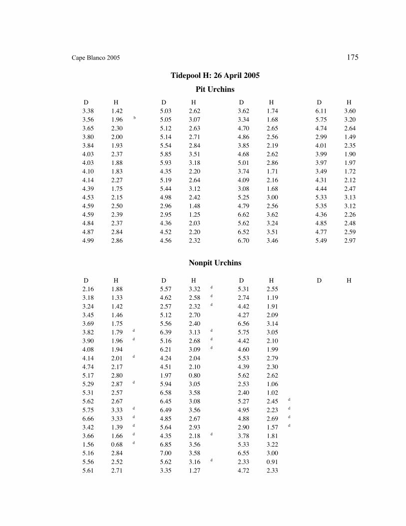
Cape Blanco 2005 175
Tidepool H: 26 April 2005
Pit Urchins
D H D H D H D H
3.38 1.42
3.56 1.96 b
3.65 2.30
3.80 2.00
3.84 1.93
4.03 2.37
4.03 1.88
4.10 1.83
4.14 2.27
4.39 1.75
4.53 2.15
4.59 2.50
4.59 2.39
4.84 2.37
4.87 2.84
4.99 2.86
5.03 2.62
5.05 3.07
5.12 2.63
5.14 2.71
5.54 2.84
5.85 3.51
5.93 3.18
4.35 2.20
5.19 2.64
5.44 3.12
4.98 2.42
2.96 1.48
2.95 1.25
4.36 2.03
4.52 2.20
4.56 2.32
3.62 1.74
3.34 1.68
4.70 2.65
4.86 2.56
3.85 2.19
4.68 2.62
5.01 2.86
3.74 1.71
4.09 2.16
3.08 1.68
5.25 3.00
4.79 2.56
6.62 3.62
5.62 3.24
6.52 3.51
6.70 3.46
6.11 3.60
5.75 3.20
4.74 2.64
2.99 1.49
4.01 2.35
3.99 1.90
3.97 1.97
3.49 1.72
4.31 2.12
4.44 2.47
5.33 3.13
5.35 3.12
4.36 2.26
4.85 2.48
4.77 2.59
5.49 2.97
Nonpit Urchins
D H D H D H D H
2.16 1.88
3.18 1.33
3.24 1.42
3.45 1.46
3.69 1.75
3.82 1.79 d
3.90 1.96 d
4.08 1.94
4.14 2.01 d
4.74 2.17
5.17 2.80
5.29 2.87 d
5.31 2.57
5.62 2.67
5.75 3.33 d
6.66 3.33 d
3.42 1.39 d
3.66 1.66 d
1.56 0.68 d
5.16 2.84
5.56 2.52
5.61 2.71
5.57 3.32 d
4.62 2.58 d
2.57 2.32 d
5.12 2.70
5.56 2.40
6.39 3.13 d
5.16 2.68 d
6.21 3.09 d
4.24 2.04
4.51 2.10
1.97 0.80
5.94 3.05
6.58 3.58
6.45 3.08
6.49 3.56
4.85 2.67
5.64 2.93
4.35 2.18 d
6.85 3.56
7.00 3.58
5.62 3.16 d
3.35 1.27
5.31 2.55
2.74 1.19
4.42 1.91
4.27 2.09
6.56 3.14
5.75 3.05
4.42 2.10
4.60 1.99
5.53 2.79
4.39 2.30
5.62 2.62
2.53 1.06
2.40 1.02
5.27 2.45 d
4.95 2.23 d
4.88 2.69 d
2.90 1.57 d
3.78 1.81
5.33 3.22
6.55 3.00
2.33 0.91
4.72 2.33
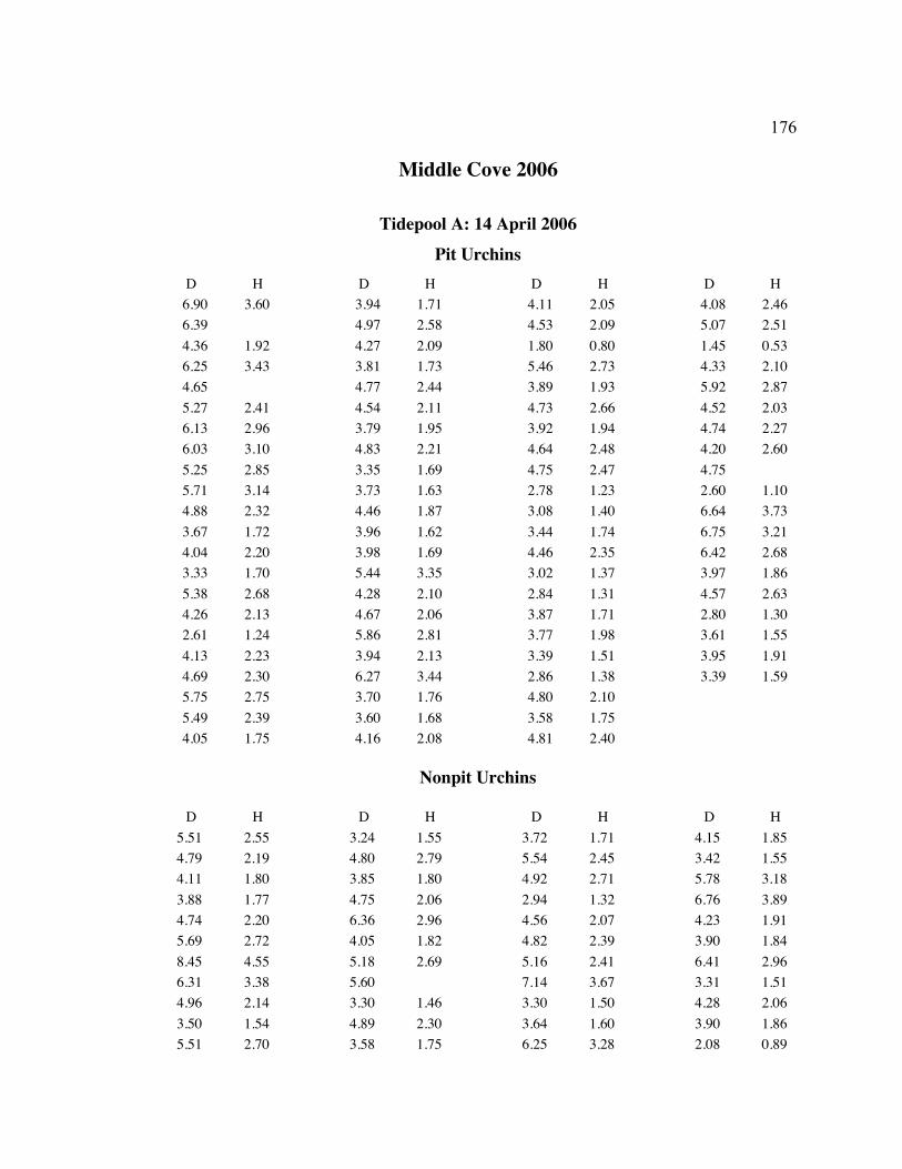
176
Middle Cove 2006
Tidepool A: 14 April 2006
Pit Urchins
D H D H D H D H
6.90 3.60
6.39
4.36 1.92
6.25 3.43
4.65
5.27 2.41
6.13 2.96
6.03 3.10
5.25 2.85
5.71 3.14
4.88 2.32
3.67 1.72
4.04 2.20
3.33 1.70
5.38 2.68
4.26 2.13
2.61 1.24
4.13 2.23
4.69 2.30
5.75 2.75
5.49 2.39
4.05 1.75
3.94 1.71
4.97 2.58
4.27 2.09
3.81 1.73
4.77 2.44
4.54 2.11
3.79 1.95
4.83 2.21
3.35 1.69
3.73 1.63
4.46 1.87
3.96 1.62
3.98 1.69
5.44 3.35
4.28 2.10
4.67 2.06
5.86 2.81
3.94 2.13
6.27 3.44
3.70 1.76
3.60 1.68
4.16 2.08
4.11 2.05
4.53 2.09
1.80 0.80
5.46 2.73
3.89 1.93
4.73 2.66
3.92 1.94
4.64 2.48
4.75 2.47
2.78 1.23
3.08 1.40
3.44 1.74
4.46 2.35
3.02 1.37
2.84 1.31
3.87 1.71
3.77 1.98
3.39 1.51
2.86 1.38
4.80 2.10
3.58 1.75
4.81 2.40
4.08 2.46
5.07 2.51
1.45 0.53
4.33 2.10
5.92 2.87
4.52 2.03
4.74 2.27
4.20 2.60
4.75
2.60 1.10
6.64 3.73
6.75 3.21
6.42 2.68
3.97 1.86
4.57 2.63
2.80 1.30
3.61 1.55
3.95 1.91
3.39 1.59
Nonpit Urchins
D H D H D H D H
5.51 2.55
4.79 2.19
4.11 1.80
3.88 1.77
4.74 2.20
5.69 2.72
8.45 4.55
6.31 3.38
4.96 2.14
3.50 1.54
5.51 2.70
3.24 1.55
4.80 2.79
3.85 1.80
4.75 2.06
6.36 2.96
4.05 1.82
5.18 2.69
5.60
3.30 1.46
4.89 2.30
3.58 1.75
3.72 1.71
5.54 2.45
4.92 2.71
2.94 1.32
4.56 2.07
4.82 2.39
5.16 2.41
7.14 3.67
3.30 1.50
3.64 1.60
6.25 3.28
4.15 1.85
3.42 1.55
5.78 3.18
6.76 3.89
4.23 1.91
3.90 1.84
6.41 2.96
3.31 1.51
4.28 2.06
3.90 1.86
2.08 0.89

Middle Cove 2006 177
D H D H D H D H
3.38 1.60
3.33 1.55
3.31 1.47
3.95 1.85
4.48 2.05
3.03 1.47
2.64 1.09
1.86 0.80
6.20
2.04 0.92
3.99 1.66
2.33 1.00
2.14 0.98
2.77 1.26
2.87 1.13
7.56 4.34
7.49 3.67
7.07 3.29
6.97 3.72
6.96 3.45
6.48 3.60
Tidepool B: 14 & 17 April 2006
Pit Urchins
D H D H D H D H
5.44 2.80
5.58 3.43
5.65 2.91
6.28 3.28
5.63 2.98
4.45 2.27
5.55 2.66
5.47 2.67
5.03 3.02
3.32
6.25 2.85
5.65 2.77
5.19 2.25
4.78 2.45
5.34 2.87
4.52 2.37
4.96 2.70
6.80 3.60
5.64 2.95
6.11 2.81
7.49 4.27
6.51 3.20
3.86 1.93
4.79 2.67
4.40
4.40 2.14
2.86 1.35
2.80 1.45
6.05 3.18
4.73 2.20
4.15 2.13
6.16 3.36
5.06 2.22
4.61 2.76
6.33 3.67
4.35 2.44
4.66 2.53
4.44 2.24
6.01 3.03
5.74 3.37
3.46 1.69
5.59 2.65
4.27 1.86
5.99 3.16
4.12 1.93
3.50 1.70
1.80 0.70
5.49 2.72
5.02 2.65
3.91 1.75
5.49 2.70
7.91 4.17
6.80 3.03
6.26 3.01
6.64 3.20
6.44 3.58
6.44 3.66
1.65 0.82
6.50 2.80
7.11 4.40
5.30
2.66 1.37
7.24
6.10 3.43
5.97 3.11
4.47 2.09
6.86 3.54
3.01 1.54
4.00 2.00
4.49 2.38
6.03 2.96
5.76 3.31
5.67 2.53
6.27 3.41
6.69 3.67
4.13 1.97
4.96 2.90
7.10
4.20 1.92
4.45 2.04
6.32 3.38
5.26 2.57
3.95 1.74
6.17 3.43
6.47 3.17
5.49 2.65
4.82 2.41
5.53 2.87
3.39 1.60
2.62 1.09
6.25 3.24
3.88 2.14
0.96 0.40
6.89 3.69
6.72 4.17
7.26 3.57
6.97 3.71
6.93 3.92
6.98 3.43
6.49 3.37
Nonpit Urchins
D H D H D H D H
6.51 3.56
6.25 3.14
5.70 3.09
5.22 2.82
4.80 2.20
3.80 1.53
6.04 2.87
6.41 3.05
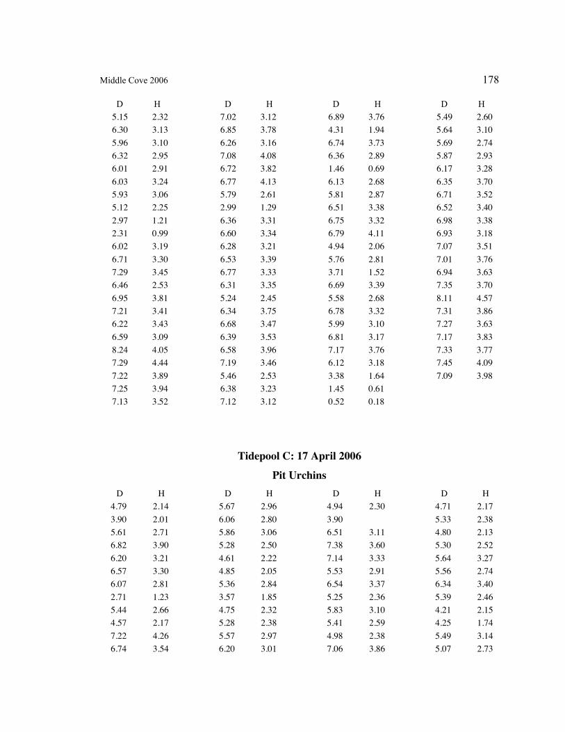
Middle Cove 2006 178
D H D H D H D H
5.15 2.32
6.30 3.13
5.96 3.10
6.32 2.95
6.01 2.91
6.03 3.24
5.93 3.06
5.12 2.25
2.97 1.21
2.31 0.99
6.02 3.19
6.71 3.30
7.29 3.45
6.46 2.53
6.95 3.81
7.21 3.41
6.22 3.43
6.59 3.09
8.24 4.05
7.29 4.44
7.22 3.89
7.25 3.94
7.13 3.52
7.02 3.12
6.85 3.78
6.26 3.16
7.08 4.08
6.72 3.82
6.77 4.13
5.79 2.61
2.99 1.29
6.36 3.31
6.60 3.34
6.28 3.21
6.53 3.39
6.77 3.33
6.31 3.35
5.24 2.45
6.34 3.75
6.68 3.47
6.39 3.53
6.58 3.96
7.19 3.46
5.46 2.53
6.38 3.23
7.12 3.12
6.89 3.76
4.31 1.94
6.74 3.73
6.36 2.89
1.46 0.69
6.13 2.68
5.81 2.87
6.51 3.38
6.75 3.32
6.79 4.11
4.94 2.06
5.76 2.81
3.71 1.52
6.69 3.39
5.58 2.68
6.78 3.32
5.99 3.10
6.81 3.17
7.17 3.76
6.12 3.18
3.38 1.64
1.45 0.61
0.52 0.18
5.49 2.60
5.64 3.10
5.69 2.74
5.87 2.93
6.17 3.28
6.35 3.70
6.71 3.52
6.52 3.40
6.98 3.38
6.93 3.18
7.07 3.51
7.01 3.76
6.94 3.63
7.35 3.70
8.11 4.57
7.31 3.86
7.27 3.63
7.17 3.83
7.33 3.77
7.45 4.09
7.09 3.98
Tidepool C: 17 April 2006
Pit Urchins
D H D H D H D H
4.79 2.14
3.90 2.01
5.61 2.71
6.82 3.90
6.20 3.21
6.57 3.30
6.07 2.81
2.71 1.23
5.44 2.66
4.57 2.17
7.22 4.26
6.74 3.54
5.67 2.96
6.06 2.80
5.86 3.06
5.28 2.50
4.61 2.22
4.85 2.05
5.36 2.84
3.57 1.85
4.75 2.32
5.28 2.38
5.57 2.97
6.20 3.01
4.94 2.30
3.90
6.51 3.11
7.38 3.60
7.14 3.33
5.53 2.91
6.54 3.37
5.25 2.36
5.83 3.10
5.41 2.59
4.98 2.38
7.06 3.86
4.71 2.17
5.33 2.38
4.80 2.13
5.30 2.52
5.64 3.27
5.56 2.74
6.34 3.40
5.39 2.46
4.21 2.15
4.25 1.74
5.49 3.14
5.07 2.73
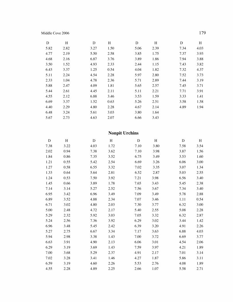
Middle Cove 2006 179
D H D H D H D H
5.82 2.82
4.77 2.19
4.68 2.16
3.50 1.52
6.43 3.37
5.11 2.24
2.33 1.04
5.88 2.47
5.44 2.61
4.55 2.12
6.69 3.37
4.40 2.29
6.48 3.24
5.67 2.73
3.27 1.50
5.50 2.58
6.87 3.76
4.93 2.33
1.25 0.54
4.54 2.28
4.78 2.36
4.09 1.81
4.45 2.11
6.88 3.46
1.52 0.63
4.80 2.28
5.61 3.03
4.63 2.07
5.06 2.39
3.85 1.75
3.89 1.86
2.44 1.15
4.04 1.82
5.97 2.80
5.71 2.89
5.65 2.57
5.11 2.21
3.53 1.59
5.26 2.51
4.67 2.14
3.80 1.64
6.66 3.43
7.34 4.03
7.37 3.93
7.94 3.88
7.43 3.82
7.32 4.37
7.52 3.73
7.44 3.19
7.45 3.71
7.71 3.91
3.33 1.41
3.58 1.58
4.89 1.94
Nonpit Urchins
D H D H D H D H
7.38 3.22
2.02 0.94
1.84 0.86
1.21 0.55
1.27 0.58
1.33 0.64
1.24 0.53
1.45 0.66
7.14 3.14
6.95 3.42
6.89 3.52
6.71 3.02
5.00 2.48
5.29 2.32
5.24 2.56
6.96 3.48
5.27 2.75
5.94 2.98
6.63 3.91
6.29 3.19
7.00 3.68
7.02 3.28
6.59 3.19
4.55 2.28
4.03 1.72
7.38 3.62
7.35 3.52
5.42 2.54
6.55 3.32
5.64 2.81
7.50 3.92
3.89 1.78
5.27 2.52
6.96 3.49
4.88 2.34
4.80 2.03
4.72 2.17
5.92 3.03
7.36 3.92
5.45 2.42
6.67 3.34
3.38 1.43
4.90 2.13
3.69 1.43
5.29 2.37
3.41 1.46
4.60 2.26
4.89 2.25
7.10 3.80
7.10 3.98
6.75 3.49
6.69 3.26
7.02 3.35
6.52 2.87
7.21 3.98
7.65 3.43
7.56 3.67
7.09 3.49
7.07 3.46
7.30 3.77
5.40 2.55
7.05 3.32
6.29 3.02
6.39 3.20
7.17 3.63
7.00 3.72
6.06 3.01
7.59 3.97
4.91 2.17
4.27 1.87
5.53 2.76
2.66 1.07
7.58 3.54
3.87 1.56
3.53 1.60
6.06 3.00
3.07 1.34
5.03 2.55
6.56 3.40
5.45 2.38
7.34 3.40
5.78 2.88
1.11 0.54
6.32 3.00
5.08 2.28
6.32 2.87
3.44 1.42
4.91 2.26
6.88 4.03
6.69 3.77
4.54 2.06
4.21 1.89
7.01 3.14
5.86 3.11
4.08 1.89
5.58 2.71
Middle Cove 2006 180
D H D H D H D H
4.80 2.27
6.91 3.75
7.03 3.29
7.08 3.69
6.76 3.21
6.02 3.02
6.25 3.22
6.64 3.59
8.67 4.50
8.30 4.86
8.29 3.40
7.71 3.95
7.61 4.42
7.57 3.69
6.54 3.78
8.54 4.38
8.11 4.12
7.63 4.23
8.10 4.07
7.76 4.09
7.63 3.60
6.71 3.58
8.07 4.14
7.63 4.17
7.83 3.81
7.64 4.29
7.77 4.33
7.71 3.92
7.17 3.76
7.51 3.46
7.69 3.84
7.67 3.88
8.26 4.29
8.17 4.17
7.67 4.03
7.63 4.01
8.10 4.08
7.63 4.11
7.63 3.73
7.70 3.58
Middle Cove 2005
Tidepool D: 20 February 2005
Pit Urchins
D H D H D H D H
6.51 3.43
5.83 3.31
4.65 2.39
3.52 1.95
5.62 3.28
7.68 3.92
6.25 2.98
7.17 3.85
3.29 1.63
5.95 3.34
1.30 b
5.85 3.25
2.67 1.29
3.33 1.56
5.55 2.79
6.67 3.62
6.77 3.19
5.56 2.62
6.52 3.22
Nonpit Urchins
D H D H D H D H
1.24 0.51
6.80 3.71
6.16 2.78
3.98 1.56
2.94 1.28
3.79 1.69
8.36 4.19
6.55 3.33
7.43 3.09
7.16 3.16
5.79 2.66
7.40 0.00
7.78 4.57
5.84 3.24
7.48 3.71
5.69 2.80
6.75 3.59
7.77 3.03
8.65 4.52
7.49 3.87
3.89 1.88
6.22 2.66
7.24 3.67
Tidepool E: Unknown 2005
Pit Urchins
D H D H D H D H
5.42 2.92
5.50 2.73
1.70 0.70
5.57 2.99
6.47 3.96
6.12 3.33
3.91 1.74
3.10 1.41
0.86 0.37
6.89 3.86
5.84 3.03
7.58 3.71
3.45 1.38
3.81 1.65
5.23 2.58
5.62 2.43
5.53 2.74
6.07 3.02
3.01 1.30
4.96 2.64
4.38 2.09
1.56 0.54
5.03 2.42
6.03 3.08
Middle Cove 2005 181
D H D H D H D H
6.15 3.37
3.62 1.58
5.43 2.60
7.12 3.65
7.41 3.76
5.69 2.57
5.56 2.55
6.43 3.17
6.35 3.26
3.08 1.31
7.36 3.95
6.64
5.46 2.58
4.86 2.23
5.15 2.52
Nonpit Urchins
D H D H D H D H
3.26 1.23
6.91 3.21
3.24 1.36
3.42 1.41
6.63 3.47
7.51 3.95
7.09 3.91
8.09 3.87
7.41 4.07
2.02 1.03
6.85 3.49
7.63 3.42
1.74 0.80
3.85 1.55
7.61 3.68
8.27 4.53
4.43 2.03
3.96 1.72
3.50 1.26
8.68 4.38
4.59 1.91
4.12 2.04
7.71 3.58
7.87 3.66
7.72 3.87
6.52 2.95
4.64 2.09
6.63 3.32
7.64 3.83
6.58 3.28
7.81 3.90
5.07
7.87
7.59 3.53
7.50 3.80
1.57 0.65
6.58 3.19
7.82 3.15
7.31 3.72
8.79 3.99
7.48 3.82
8.24 3.85
7.63 3.94
6.63 3.17
5.66 2.58
7.90 4.21
6.93 3.26
4.38 1.93
7.05 3.31
6.25 3.44
6.90 3.28
6.13 3.29
8.36 4.41
6.34 3.01
6.49 2.73
8.80 4.15
8.68 3.88
7.63 3.13
3.98 1.68
6.32 2.78
5.04 1.97
3.29 1.11
3.22 1.19
6.60 2.79
7.35 3.64
7.26 3.44
1.78 0.62
3.25 1.25
6.79 3.03
6.90 3.56
6.24 2.82
6.83 3.54
4.12 1.85
7.48 3.73
7.49 3.73
5.95 2.89
3.58 1.51
7.12 3.45
6.03 2.63
6.16 3.14
6.13 2.79
4.35 1.66
5.35 2.01
3.79 1.82
1.23 0.48
5.45 2.32
7.84 4.43
4.23 1.68
7.67 3.88
1.81 0.59
Tidepool F: 10 May 2005
Pit Urchins
D H D H D H D H
6.32 3.37
6.34 3.19
6.05 3.30
6.02 3.20
7.15 3.86
5.41 2.96
5.52 2.71
5.46 2.47
6.85 3.57
5.83 2.76
2.92 u
4.26 1.96
6.82 3.66
5.21 2.40
5.57 2.78
5.31 2.92
7.09 3.46
5.73 2.83
6.42 3.19
5.29 2.78
5.79 2.63
6.11 3.04
5.85 2.84
6.54 3.23
3.79 1.83
1.54 0.59
5.89 2.89
5.11 2.58
3.50 2.14
5.22 2.46
5.20 2.58
4.53 2.21
5.05 2.57
4.36 1.94
4.34 2.09
3.68 1.66
3.21 1.23
5.01 2.71
4.37 1.98
4.59 2.06
4.16 2.09
3.72 1.56
4.96 2.26
4.75 2.31
Middle Cove 2005 182
D H D H D H D H
4.42 2.04
4.41 2.05
3.35 1.58
4.81 2.37
3.78 1.86
4.05 1.94
2.90 1.20
4.35 1.95
4.30 2.01
3.98 1.69
4.07 1.59
4.87 2.56
4.92 2.30
4.48 2.10
3.27 2.18
4.60 2.33
4.50 2.57
1.80 0.74
5.38 2.95
3.93 1.68
5.15 2.40
5.23 2.72
2.87 1.10
4.53 2.25
5.50 3.01
4.58 2.00
5.22 2.51
4.98 2.01
2.77 1.11
5.27 2.62
5.29 2.64
4.73 2.11
2.99 1.26
6.04 2.74
1.88 0.79
4.52 2.29
4.20 1.88
5.62 2.97
5.32 2.55
4.96 2.78
4.78 2.52
4.62 2.21
5.55 2.78
4.20 1.85
4.64 1.85
4.64 2.09
4.63 2.26
4.85 2.18
2.78 1.33
4.85 2.34
0.67 0.29
4.88 2.43
4.02 2.05
4.70 2.41
1.45 0.57
4.60 2.44
3.49 1.77
1.45 0.59
4.46 2.03
Nonpit Urchins
D H D H D H D H
2.89 1.32
7.60 3.83 d
6.99 3.45 d
6.21 3.11 d
6.54 3.18 d
6.31 3.14
6.58 3.59
7.26 3.78
5.95 2.90
6.52 3.70 d
3.48 1.50 d
7.08 3.38 d
6.01 3.26
5.88 3.01 d
6.09 2.87 d
4.96 2.71
5.70 2.78
5.55 2.79 d
6.06 3.32
7.58 3.81
6.23 2.96
6.40 3.28
6.40 2.61 d
2.87 1.08
4.50 1.74
3.86 1.62
6.71 3.24
5.76 2.86
6.47 3.49
6.60 3.41
1.25 0.49
7.18 4.20
5.68 2.73
6.99 3.51
6.26 2.88
4.32 1.66
6.03 2.74
7.66 3.98
7.75 4.58
5.51 2.86
6.97 3.55
5.37 2.46
6.54 3.25
6.68 3.69
6.01 2.88
4.92 2.08
5.50 2.47
6.78 3.54
6.80 3.44
5.36 2.61
5.46 2.45
3.92 1.78
5.56 2.52
6.48 3.11 d
6.26 3.00
7.40 3.46
6.90 3.15
5.81 3.01
6.87 3.20
7.50 3.44
5.32 2.51
6.52 3.40
6.82 3.21
5.96 2.79
5.28 2.84
3.19 1.80
8.04 4.24
6.97 3.28
6.26 3.22
6.46 3.14
6.96 2.81
2.88 1.15
2.65 1.11
4.72 2.33
4.85 2.05
2.98 1.18
2.48 1.01
5.28 2.44
3.60 1.52
2.48 1.03
6.79 3.02
2.56 1.00
5.65 2.86
3.56 1.64
6.55 3.31
6.74 3.59
5.10 2.48
6.35 3.10
6.45 3.17
5.60 2.85
5.76 2.90
4.63 2.32
5.63 2.54
0.88 0.36
1.02 0.44
2.88 1.22
1.93 0.71
3.57 1.44
3.26 1.48
6.37 2.96
5.63 2.72
6.68 3.28
5.18 2.73
5.55 2.44
5.90 2.86
6.59 2.98
6.59 2.97
5.16 2.67
5.71 2.70
5.62 2.63
5.26 2.44
2.87 1.33
1.47 0.55
1.12 0.43
4.81 2.26
2.99 1.16
5.94 2.97
3.63 1.50
5.10 2.28
5.12 2.46

Middle Cove 2005 183
D H D H D H D H
5.17 2.53
6.09 2.96
6.32 3.23
5.92 3.24
2.57 1.05
3.87 1.73
3.17 1.38
2.99 1.26
2.96 1.12
2.90 1.12
2.39 0.99
5.98 3.10
5.75 2.99
5.27 2.34
2.94 1.55
Tidepool G: 20 February 2006
Pit Urchins
D H D H D H D H
5.42 2.69
6.15 3.64
4.54 2.18
6.23 3.45
6.54 3.65
6.62 3.27
3.84 2.09
3.46 1.58
7.11 3.61
6.57 3.41
3.34 1.70
4.04 1.62
5.97 3.03
4.42 2.24
4.65 2.33
7.15 3.68
4.58 2.44
3.79 1.92
0.94 0.41
5.22 2.98
5.08 2.34
7.84 4.36
3.65 1.72
8.17 4.17
5.12 2.81
Nonpit Urchins
D H D H D H D H
4.83 2.25
1.37 0.58
3.44 1.61
1.65 0.66
6.97 3.83
6.62 3.53
7.45 4.36
2.58 1.04
0.94 0.41
Tidepool H: 9 May 2005
Pit Urchins
D H D H D H D H
2.47 1.19
2.48 1.08
3.07 1.60
3.36 1.46
3.42 1.46
3.77 1.57
3.81 1.86
3.95 1.95
3.96 1.98
3.99 1.99
4.03 1.91
4.20 1.83
4.28 2.30
4.33 2.10
4.37 1.83
4.41 2.20
4.57 2.20
4.66 2.48
4.69 2.39
4.77 2.53
4.77 2.51
4.82 2.47
4.82 2.46
4.98 2.83
4.99 2.36
5.18 2.61
5.19 2.59
5.25 2.48
5.29 2.98
5.31 2.63
5.31 2.45
5.32 2.73
5.36 2.56
5.38 2.72
5.39 2.78
5.49 3.17 u
5.53 2.64
5.54 2.90
5.57 2.79
5.64 3.30
5.65 2.66
5.65 2.94
5.69 3.63
5.69 u
5.70 3.11
5.81 2.78
5.83 3.11
5.83 3.21
5.96 2.90
6.01 2.89
6.06 3.15
6.10 3.24
6.14 3.75
6.17 2.82
6.17 3.14
6.22 2.96
6.25 3.18
6.26 3.51
6.34 3.64
6.36 3.52
6.53 3.00
6.56 2.94
6.57 3.14
6.60 3.10
6.62 3.42
6.72 3.31
6.73 2.97
6.74 3.11

Middle Cove 2005 184
D H D H D H
6.74 3.59
6.81 3.37
6.88 3.65
6.96 3.29
7.35 4.08
Nonpit Urchins
D H D H D H D H
0.69 0.25
1.04 0.39
2.79 1.21
2.86 1.22 d
3.32 1.41 d
3.65 1.53
3.86 1.70
4.30 2.37 d
4.78 2.41
5.53 3.10
5.58 2.77 d
5.64 2.91 d
5.67 2.73
5.69 2.90
5.90 2.90
5.98 3.03
6.01 3.32
6.04 2.98
6.06 3.20
6.23 3.42
6.26 3.37
6.34 3.04
6.50 3.13
6.54 3.28
6.58 3.38
6.59 3.29
6.64 2.98
6.70 3.35
6.72 3.60
6.74 3.39
6.76 3.35
6.76 3.84
6.77 3.36
6.82 3.70
6.91 3.32 d
7.02 3.47
7.38 3.47
South Cove 2006
Tidepool A: 1 April 2006
Pit Urchins
D H D H D H D H
6.25 3.32
5.84 3.17
5.02 2.59
4.26 2.07
5.43 2.98
4.91 2.69
6.10 3.53
5.91 3.22
4.30 2.02
5.30 3.22
6.32 3.59
4.67 2.15
4.71 2.88
6.00 3.40
4.35 2.11
5.75 2.95
2.92 1.31
1.82 0.76
4.21 1.86
6.05 3.10
6.21 3.50
4.97 2.71
5.60 2.97
6.14 3.15
4.90 2.41
4.79 2.77
5.82 3.08
5.82 3.26
5.64 2.97
5.52 3.14
5.87 2.96
5.91 3.11
5.49 3.18
4.69 2.22
5.56 2.95
4.95 2.57
5.07 2.57
5.10 2.46
4.89 2.60
4.61 2.21
5.47 3.28
5.71 3.33
3.30 1.70
5.86 3.43
4.53 2.39
6.35 3.35
6.07 3.17
4.93 2.62
3.54 1.68
5.45 3.09
1.83 0.82
5.06 2.80
3.50 1.59
4.82 2.51
5.92 2.90
3.70 1.80
5.46 3.33
5.89 3.05
5.25 2.65
3.13 1.64
South Cove 2005 185
Nonpit Urchins
D H D H D H D H
6.49 3.33
6.31 3.17
5.64 2.64
6.10 3.31
6.76 3.52
5.63 3.07
3.77 1.82
5.79 2.94
6.42 3.61
7.23 3.81
5.98 3.69
5.21 2.59
5.96 3.19
5.86 3.17
5.56 2.91
5.57 3.17
7.08 3.99
6.49 3.40
6.91 3.35
5.71 3.23
4.76 2.57
5.68 2.73
6.42 3.26
5.71 3.09
1.12 0.59
5.53 2.92
6.52 3.20
5.85 3.02
4.27 1.94
6.97 3.29
6.90 3.29
5.71 3.35
5.12 2.48
5.37 2.68
7.38 3.93
6.11 2.93
6.56 3.58
5.94 2.85
6.17 3.54
6.34 2.80
5.65 3.03
5.60 2.70
5.05 2.94
6.20 3.59
2.31 1.00
0.93 0.43
6.02 3.01
6.25 3.26
Tidepool B: 1 April 2006
Pit Urchins
D H D H D H D H
6.30 3.33
6.85 3.67
5.42 2.96
6.58 3.82
4.83 2.55
5.40
5.60 2.84
6.11 3.00
4.70 2.42
4.65 2.20
5.85 2.74
5.38 2.90
5.45 2.81
6.13 3.48
5.79 3.03
5.40 2.37
6.71 3.51
5.87 3.41
4.90 2.46
5.88 3.24
5.95 3.08
5.02 2.43
5.71 3.46
6.27 3.00
3.11 1.38
3.61 2.38
5.80
4.37 2.30
5.08 2.68
5.61 3.35
4.85 2.78
4.63 2.57
6.10 3.24
3.40 1.60
4.66 2.77
4.62 2.37
3.58 1.69
6.81 3.60
6.29 3.33
5.00 2.39
6.16 3.44
5.89 3.29
5.26 2.88
3.89 1.87
5.71 2.66
6.46 3.48
6.48 3.05
4.26 2.17
5.04 2.75
5.38 2.76
2.97 1.15
3.84
4.17 2.10
5.78 3.28
Nonpit Urchins
D H D H D H D H
6.63 3.76
6.28 3.84
4.85 2.40
7.81 3.95
6.45 3.43
6.77 3.63
4.99 2.26
3.60 1.90
6.27 3.28
6.05 3.20
5.99 3.31
3.63 1.51
4.66 2.20
3.82 2.08
7.22 4.18
7.72 3.82
0.82 0.33
6.33 2.99
4.50 2.30
6.83 3.17
3.68 1.61
5.66 3.52
2.88 1.51
7.13 3.52
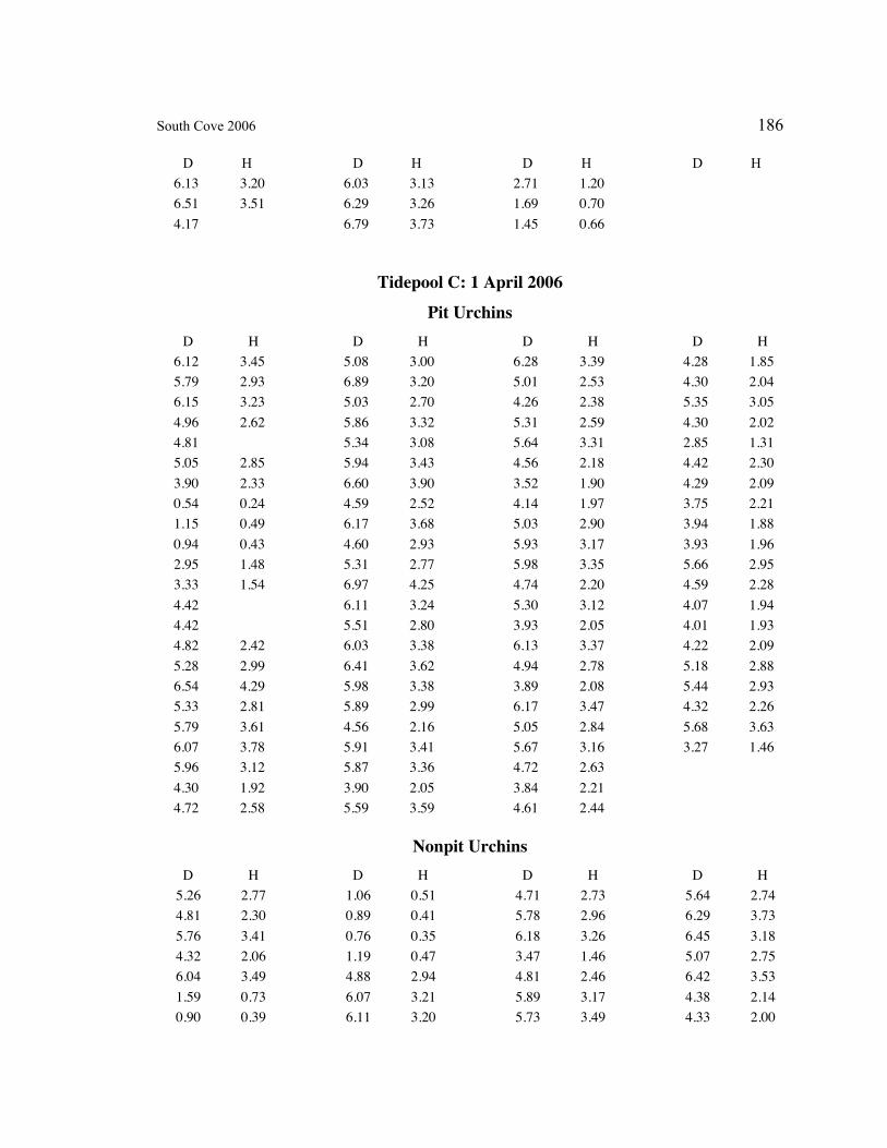
South Cove 2006 186
D H D H D H D H
6.13 3.20
6.51 3.51
4.17
6.03 3.13
6.29 3.26
6.79 3.73
2.71 1.20
1.69 0.70
1.45 0.66
Tidepool C: 1 April 2006
Pit Urchins
D H D H D H D H
6.12 3.45
5.79 2.93
6.15 3.23
4.96 2.62
4.81
5.05 2.85
3.90 2.33
0.54 0.24
1.15 0.49
0.94 0.43
2.95 1.48
3.33 1.54
4.42
4.42
4.82 2.42
5.28 2.99
6.54 4.29
5.33 2.81
5.79 3.61
6.07 3.78
5.96 3.12
4.30 1.92
4.72 2.58
5.08 3.00
6.89 3.20
5.03 2.70
5.86 3.32
5.34 3.08
5.94 3.43
6.60 3.90
4.59 2.52
6.17 3.68
4.60 2.93
5.31 2.77
6.97 4.25
6.11 3.24
5.51 2.80
6.03 3.38
6.41 3.62
5.98 3.38
5.89 2.99
4.56 2.16
5.91 3.41
5.87 3.36
3.90 2.05
5.59 3.59
6.28 3.39
5.01 2.53
4.26 2.38
5.31 2.59
5.64 3.31
4.56 2.18
3.52 1.90
4.14 1.97
5.03 2.90
5.93 3.17
5.98 3.35
4.74 2.20
5.30 3.12
3.93 2.05
6.13 3.37
4.94 2.78
3.89 2.08
6.17 3.47
5.05 2.84
5.67 3.16
4.72 2.63
3.84 2.21
4.61 2.44
4.28 1.85
4.30 2.04
5.35 3.05
4.30 2.02
2.85 1.31
4.42 2.30
4.29 2.09
3.75 2.21
3.94 1.88
3.93 1.96
5.66 2.95
4.59 2.28
4.07 1.94
4.01 1.93
4.22 2.09
5.18 2.88
5.44 2.93
4.32 2.26
5.68 3.63
3.27 1.46
Nonpit Urchins
D H D H D H D H
5.26 2.77
4.81 2.30
5.76 3.41
4.32 2.06
6.04 3.49
1.59 0.73
0.90 0.39
1.06 0.51
0.89 0.41
0.76 0.35
1.19 0.47
4.88 2.94
6.07 3.21
6.11 3.20
4.71 2.73
5.78 2.96
6.18 3.26
3.47 1.46
4.81 2.46
5.89 3.17
5.73 3.49
5.64 2.74
6.29 3.73
6.45 3.18
5.07 2.75
6.42 3.53
4.38 2.14
4.33 2.00
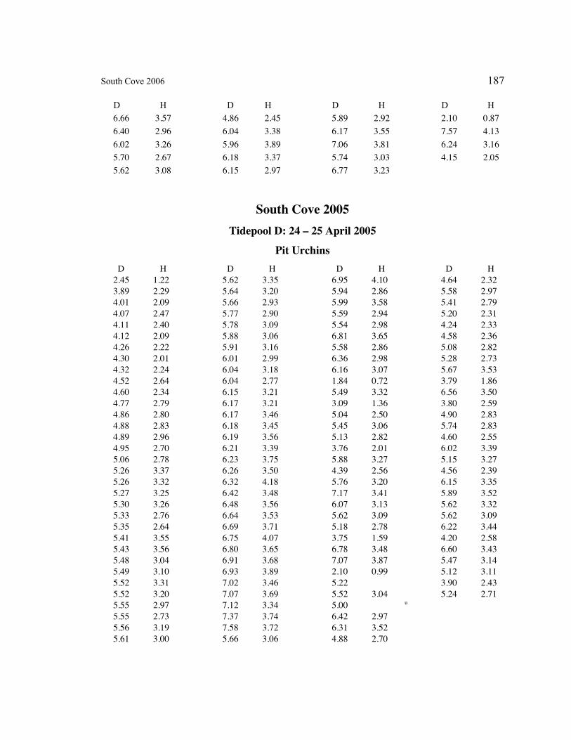
South Cove 2006 187
D H D H D H D H
6.66 3.57
6.40 2.96
6.02 3.26
5.70 2.67
5.62 3.08
4.86 2.45
6.04 3.38
5.96 3.89
6.18 3.37
6.15 2.97
5.89 2.92
6.17 3.55
7.06 3.81
5.74 3.03
6.77 3.23
2.10 0.87
7.57 4.13
6.24 3.16
4.15 2.05
South Cove 2005
Tidepool D: 24 – 25 April 2005
Pit Urchins
D H D H D H D H
2.45 1.22
3.89 2.29
4.01 2.09
4.07 2.47
4.11 2.40
4.12 2.09
4.26 2.22
4.30 2.01
4.32 2.24
4.52 2.64
4.60 2.34
4.77 2.79
4.86 2.80
4.88 2.83
4.89 2.96
4.95 2.70
5.06 2.78
5.26 3.37
5.26 3.32
5.27 3.25
5.30 3.26
5.33 2.76
5.35 2.64
5.41 3.55
5.43 3.56
5.48 3.04
5.49 3.10
5.52 3.31
5.52 3.20
5.55 2.97
5.55 2.73
5.56 3.19
5.61 3.00
5.62 3.35
5.64 3.20
5.66 2.93
5.77 2.90
5.78 3.09
5.88 3.06
5.91 3.16
6.01 2.99
6.04 3.18
6.04 2.77
6.15 3.21
6.17 3.21
6.17 3.46
6.18 3.45
6.19 3.56
6.21 3.39
6.23 3.75
6.26 3.50
6.32 4.18
6.42 3.48
6.48 3.56
6.64 3.53
6.69 3.71
6.75 4.07
6.80 3.65
6.91 3.68
6.93 3.89
7.02 3.46
7.07 3.69
7.12 3.34
7.37 3.74
7.58 3.72
5.66 3.06
6.95 4.10
5.94 2.86
5.99 3.58
5.59 2.94
5.54 2.98
6.81 3.65
5.58 2.86
6.36 2.98
6.16 3.07
1.84 0.72
5.49 3.32
3.09 1.36
5.04 2.50
5.45 3.06
5.13 2.82
3.76 2.01
5.88 3.27
4.39 2.56
5.76 3.20
7.17 3.41
6.07 3.13
5.62 3.09
5.18 2.78
3.75 1.59
6.78 3.48
7.07 3.87
2.10 0.99
5.22
5.52 3.04
5.00 u
6.42 2.97
6.31 3.52
4.88 2.70
4.64 2.32
5.58 2.97
5.41 2.79
5.20 2.31
4.24 2.33
4.58 2.36
5.08 2.82
5.28 2.73
5.67 3.53
3.79 1.86
6.56 3.50
3.80 2.59
4.90 2.83
5.74 2.83
4.60 2.55
6.02 3.39
5.15 3.27
4.56 2.39
6.15 3.35
5.89 3.52
5.62 3.32
5.62 3.09
6.22 3.44
4.20 2.58
6.60 3.43
5.47 3.14
5.12 3.11
3.90 2.43
5.24 2.71
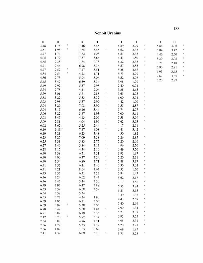
188Nonpit Urchins
D H D H D H D H
3.48 1.78 d
3.51 1.98 d
3.77 1.74
4.05 1.79
4.65 2.38
4.71 2.46
4.77 2.52 d
4.84 2.54 d
4.86 2.73
5.45 3.47
5.49 2.92
5.74 2.78
5.79 3.01
5.88 3.22
5.93 2.98
5.94 3.29
5.94 3.15
5.96 3.22
5.98 3.45
5.99 2.81
6.02 3.62
6.10 3.18 d
6.19 3.21
6.23 3.27
6.25 3.31
6.27 3.46
6.28 3.15
6.40 3.38
6.40 4.00
6.40 2.54
6.41 3.52
6.41 4.21
6.43 3.37
6.46 3.24
6.46 3.47
6.49 2.97
6.53 3.59
6.54 3.58
6.55 3.77
6.59 4.05
6.69 3.99 d
6.70 3.49
6.91 3.89
7.12 3.70 d
7.34 3.88
7.36 4.22
7.36 4.02
7.41 4.39
7.46 3.45
7.65 3.45 d
7.82 4.08
7.37 3.66
1.84 0.78
6.98 3.36
7.17 3.51
4.23 1.71
5.94 3.06
6.39 3.34
5.57 2.98
4.41 2.06 d
5.61 2.88 d
5.33 3.32 d
5.57 2.99 d
7.98 3.99 d
6.16 3.44 d
3.87 1.93 d
4.13 2.06 d
4.04 1.96 d
5.25 2.44 d
7.47 4.08 d
6.23 3.48 d
7.09 3.58 d
5.83 2.75 d
5.84 3.13 d
4.34 2.10 d
6.51 3.51 d
6.37 3.59 d
6.80 3.71 d
6.41 3.40 d
8.64 4.67 d
6.31 3.23
6.62 3.47
5.44 3.30
6.47 3.88
6.68 3.59
5.34
4.24 1.90
6.11 3.03
5.38 3.05
5.68 2.94 d
6.19 3.35
5.82 3.37 d
4.76 2.71
5.33 2.79
1.63 0.68
6.09 3.20 d
6.59 3.79 d
6.62 3.33 d
6.51 3.33
4.43 1.80 d
6.32 3.33 d
5.57 2.85 d
5.28 2.68
5.73 2.79 d
5.52 2.96 d
3.98 1.79 d
2.40 0.94
5.38 2.65 d
5.65 2.95 d
6.00 3.04 d
4.42 1.90 d
5.55 2.87 d
5.74 2.97 d
7.00 3.61
5.58 3.09 d
5.62 3.03 d
4.17 2.01
6.41 3.42 d
4.30 1.82
5.26 2.85 d
5.20 2.66
4.96 2.70 d
6.49 3.50 d
3.93 1.97 d
5.20 2.31 d
5.88 3.17 d
6.30 3.04 d
3.53 1.70 d
2.94 1.43 d
5.62 3.17 d
7.17 3.56 d
6.55 3.84 d
6.21 3.15 d
3.39 1.35 d
4.43 2.58 d
5.40 2.66 d
2.90 1.34 d
5.73 3.07 d
6.95 3.55 d
4.95 3.31 d
6.20 3.21 d
3.69 1.95
5.71 3.23 d
5.84 3.06 d
5.84 3.42 d
4.46 2.60 d
5.39 3.08 d
3.78 2.18 d
5.90 2.91 d
6.95 3.63 d
7.67 3.85 d
5.20 2.87
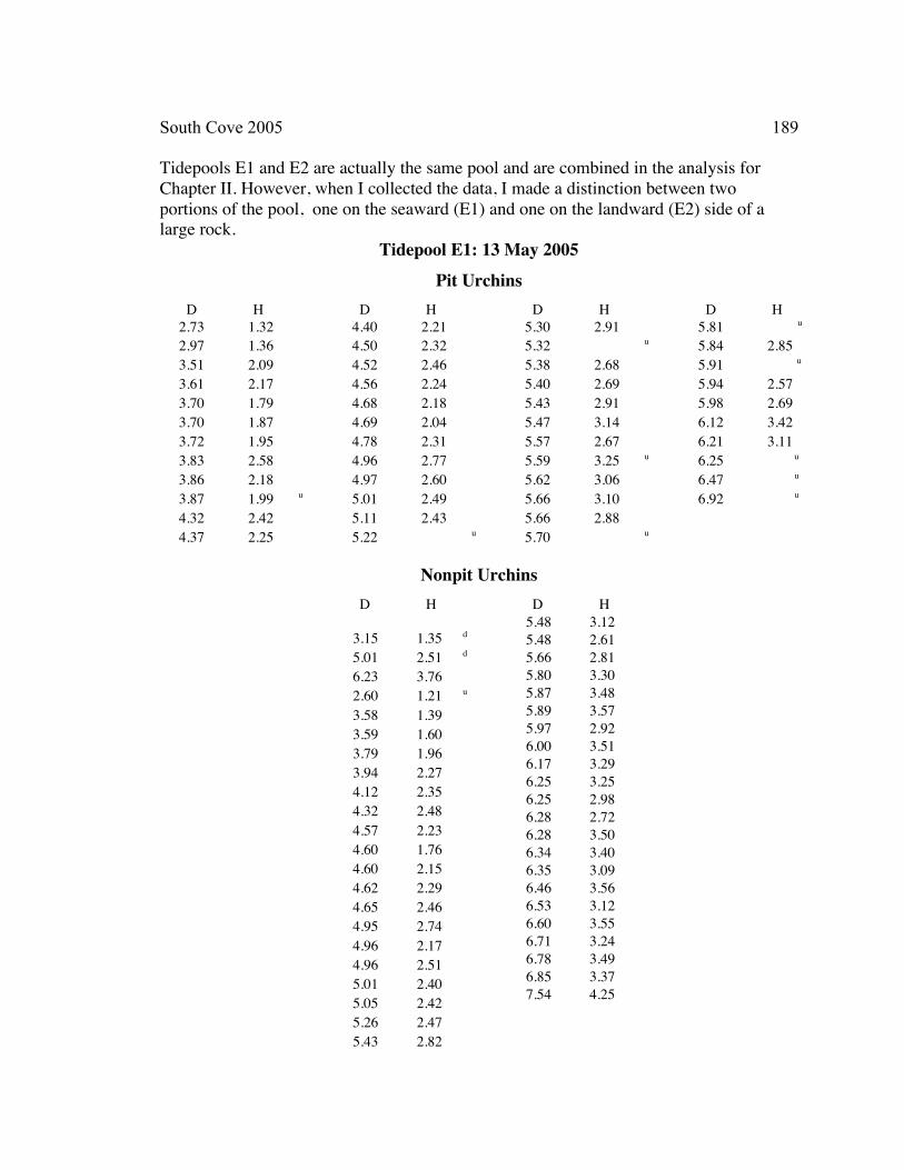
South Cove 2005 189
Tidepools E1 and E2 are actually the same pool and are combined in the analysis for
Chapter II. However, when I collected the data, I made a distinction between two
portions of the pool, one on the seaward (E1) and one on the landward (E2) side of a
large rock.
Tidepool E1: 13 May 2005
Pit Urchins
D H D H D H D H
2.73 1.32
2.97 1.36
3.51 2.09
3.61 2.17
3.70 1.79
3.70 1.87
3.72 1.95
3.83 2.58
3.86 2.18
3.87 1.99 u
4.32 2.42
4.37 2.25
4.40 2.21
4.50 2.32
4.52 2.46
4.56 2.24
4.68 2.18
4.69 2.04
4.78 2.31
4.96 2.77
4.97 2.60
5.01 2.49
5.11 2.43
5.22 u
5.30 2.91
5.32 u
5.38 2.68
5.40 2.69
5.43 2.91
5.47 3.14
5.57 2.67
5.59 3.25 u
5.62 3.06
5.66 3.10
5.66 2.88
5.70 u
5.81 u
5.84 2.85
5.91 u
5.94 2.57
5.98 2.69
6.12 3.42
6.21 3.11
6.25 u
6.47 u
6.92 u
Nonpit Urchins
D H D H
3.15 1.35 d
5.01 2.51 d
6.23 3.76
2.60 1.21 u
3.58 1.39
3.59 1.60
3.79 1.96
3.94 2.27
4.12 2.35
4.32 2.48
4.57 2.23
4.60 1.76
4.60 2.15
4.62 2.29
4.65 2.46
4.95 2.74
4.96 2.17
4.96 2.51
5.01 2.40
5.05 2.42
5.26 2.47
5.43 2.82
5.48 3.12
5.48 2.61
5.66 2.81
5.80 3.30
5.87 3.48
5.89 3.57
5.97 2.92
6.00 3.51
6.17 3.29
6.25 3.25
6.25 2.98
6.28 2.72
6.28 3.50
6.34 3.40
6.35 3.09
6.46 3.56
6.53 3.12
6.60 3.55
6.71 3.24
6.78 3.49
6.85 3.37
7.54 4.25
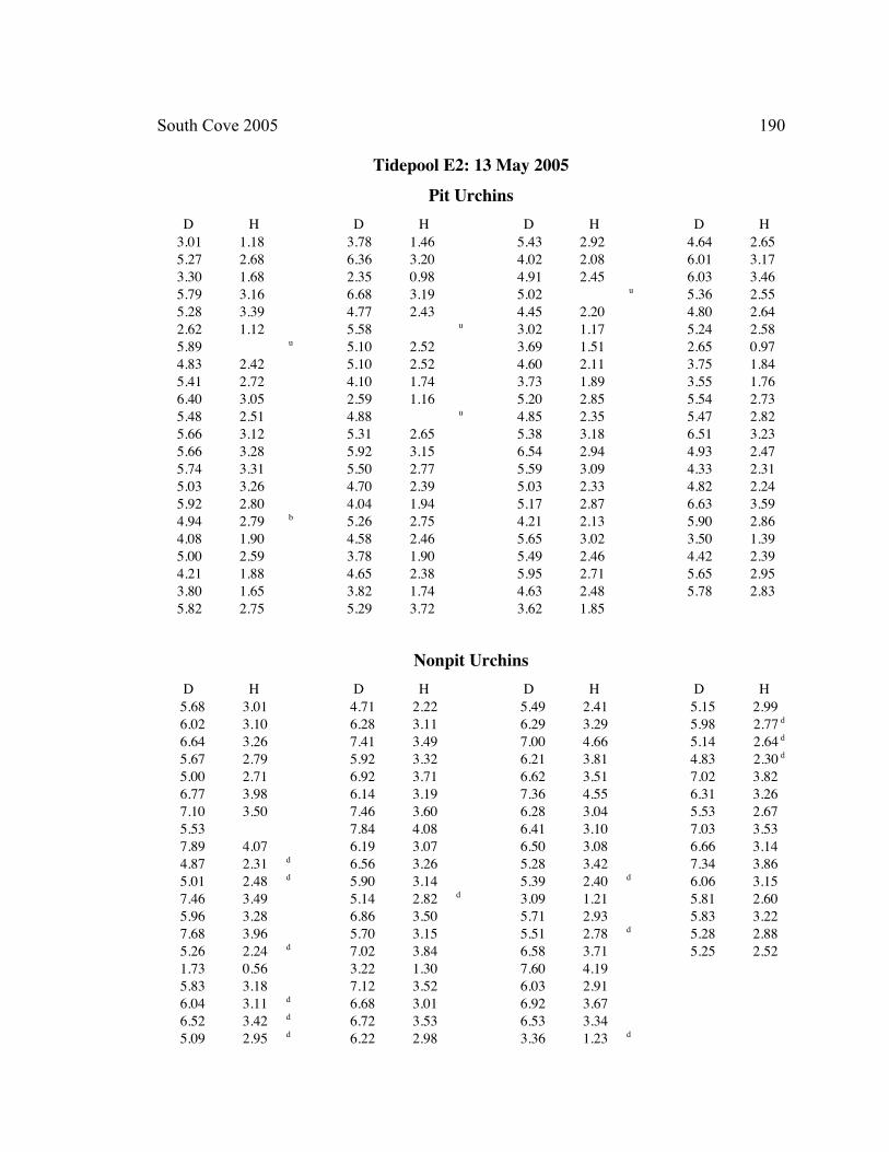
South Cove 2005 190
Tidepool E2: 13 May 2005
Pit Urchins
D H D H D H D H
3.01 1.18
5.27 2.68
3.30 1.68
5.79 3.16
5.28 3.39
2.62 1.12
5.89 u
4.83 2.42
5.41 2.72
6.40 3.05
5.48 2.51
5.66 3.12
5.66 3.28
5.74 3.31
5.03 3.26
5.92 2.80
4.94 2.79 b
4.08 1.90
5.00 2.59
4.21 1.88
3.80 1.65
5.82 2.75
3.78 1.46
6.36 3.20
2.35 0.98
6.68 3.19
4.77 2.43
5.58 u
5.10 2.52
5.10 2.52
4.10 1.74
2.59 1.16
4.88 u
5.31 2.65
5.92 3.15
5.50 2.77
4.70 2.39
4.04 1.94
5.26 2.75
4.58 2.46
3.78 1.90
4.65 2.38
3.82 1.74
5.29 3.72
5.43 2.92
4.02 2.08
4.91 2.45
5.02 u
4.45 2.20
3.02 1.17
3.69 1.51
4.60 2.11
3.73 1.89
5.20 2.85
4.85 2.35
5.38 3.18
6.54 2.94
5.59 3.09
5.03 2.33
5.17 2.87
4.21 2.13
5.65 3.02
5.49 2.46
5.95 2.71
4.63 2.48
3.62 1.85
4.64 2.65
6.01 3.17
6.03 3.46
5.36 2.55
4.80 2.64
5.24 2.58
2.65 0.97
3.75 1.84
3.55 1.76
5.54 2.73
5.47 2.82
6.51 3.23
4.93 2.47
4.33 2.31
4.82 2.24
6.63 3.59
5.90 2.86
3.50 1.39
4.42 2.39
5.65 2.95
5.78 2.83
Nonpit Urchins
D H D H D H D H
5.68 3.01
6.02 3.10
6.64 3.26
5.67 2.79
5.00 2.71
6.77 3.98
7.10 3.50
5.53
7.89 4.07
4.87 2.31 d
5.01 2.48 d
7.46 3.49
5.96 3.28
7.68 3.96
5.26 2.24 d
1.73 0.56
5.83 3.18
6.04 3.11 d
6.52 3.42 d
5.09 2.95 d
4.71 2.22
6.28 3.11
7.41 3.49
5.92 3.32
6.92 3.71
6.14 3.19
7.46 3.60
7.84 4.08
6.19 3.07
6.56 3.26
5.90 3.14
5.14 2.82 d
6.86 3.50
5.70 3.15
7.02 3.84
3.22 1.30
7.12 3.52
6.68 3.01
6.72 3.53
6.22 2.98
5.49 2.41
6.29 3.29
7.00 4.66
6.21 3.81
6.62 3.51
7.36 4.55
6.28 3.04
6.41 3.10
6.50 3.08
5.28 3.42
5.39 2.40 d
3.09 1.21
5.71 2.93
5.51 2.78 d
6.58 3.71
7.60 4.19
6.03 2.91
6.92 3.67
6.53 3.34
3.36 1.23 d
5.15 2.99
5.98 2.77 d
5.14 2.64 d
4.83 2.30 d
7.02 3.82
6.31 3.26
5.53 2.67
7.03 3.53
6.66 3.14
7.34 3.86
6.06 3.15
5.81 2.60
5.83 3.22
5.28 2.88
5.25 2.52
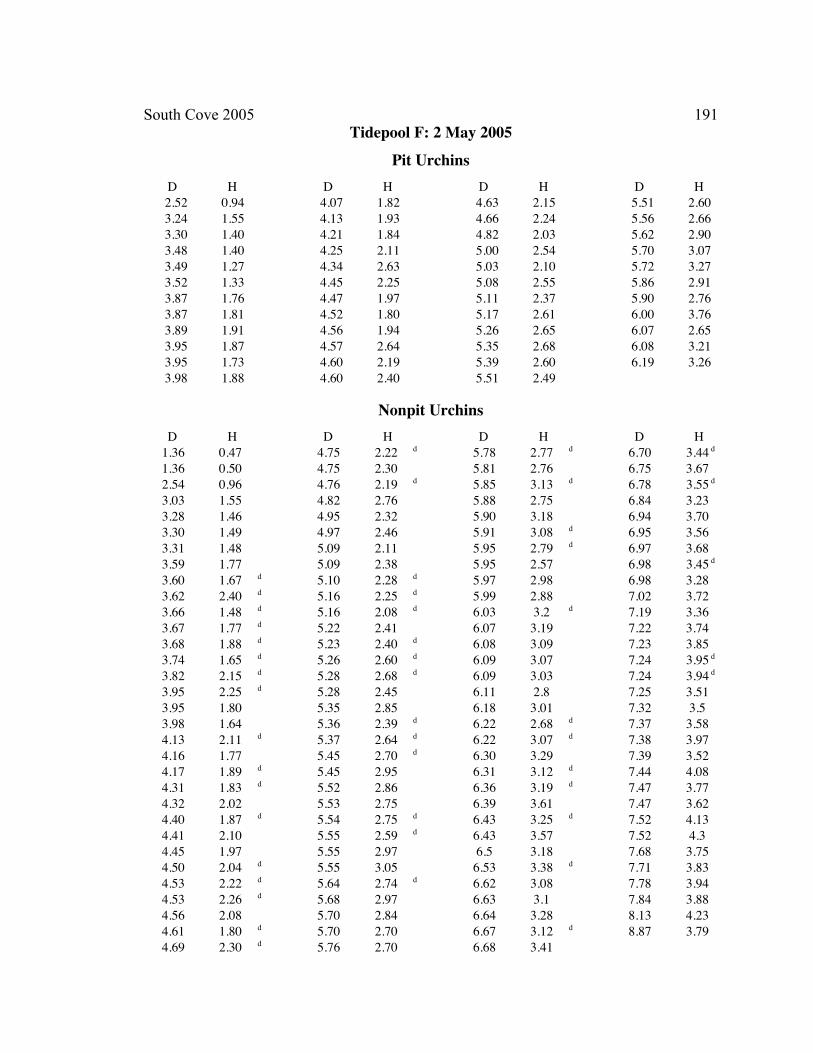
South Cove 2005 191Tidepool F: 2 May 2005
Pit Urchins
D H D H D H D H
2.52 0.94
3.24 1.55
3.30 1.40
3.48 1.40
3.49 1.27
3.52 1.33
3.87 1.76
3.87 1.81
3.89 1.91
3.95 1.87
3.95 1.73
3.98 1.88
4.07 1.82
4.13 1.93
4.21 1.84
4.25 2.11
4.34 2.63
4.45 2.25
4.47 1.97
4.52 1.80
4.56 1.94
4.57 2.64
4.60 2.19
4.60 2.40
4.63 2.15
4.66 2.24
4.82 2.03
5.00 2.54
5.03 2.10
5.08 2.55
5.11 2.37
5.17 2.61
5.26 2.65
5.35 2.68
5.39 2.60
5.51 2.49
5.51 2.60
5.56 2.66
5.62 2.90
5.70 3.07
5.72 3.27
5.86 2.91
5.90 2.76
6.00 3.76
6.07 2.65
6.08 3.21
6.19 3.26
Nonpit Urchins
D H D H D H D H
1.36 0.47
1.36 0.50
2.54 0.96
3.03 1.55
3.28 1.46
3.30 1.49
3.31 1.48
3.59 1.77
3.60 1.67 d
3.62 2.40 d
3.66 1.48 d
3.67 1.77 d
3.68 1.88 d
3.74 1.65 d
3.82 2.15 d
3.95 2.25 d
3.95 1.80
3.98 1.64
4.13 2.11 d
4.16 1.77
4.17 1.89 d
4.31 1.83 d
4.32 2.02
4.40 1.87 d
4.41 2.10
4.45 1.97
4.50 2.04 d
4.53 2.22 d
4.53 2.26 d
4.56 2.08
4.61 1.80 d
4.69 2.30 d
4.75 2.22 d
4.75 2.30
4.76 2.19 d
4.82 2.76
4.95 2.32
4.97 2.46
5.09 2.11
5.09 2.38
5.10 2.28 d
5.16 2.25 d
5.16 2.08 d
5.22 2.41
5.23 2.40 d
5.26 2.60 d
5.28 2.68 d
5.28 2.45
5.35 2.85
5.36 2.39 d
5.37 2.64 d
5.45 2.70 d
5.45 2.95
5.52 2.86
5.53 2.75
5.54 2.75 d
5.55 2.59 d
5.55 2.97
5.55 3.05
5.64 2.74 d
5.68 2.97
5.70 2.84
5.70 2.70
5.76 2.70
5.78 2.77 d
5.81 2.76
5.85 3.13 d
5.88 2.75
5.90 3.18
5.91 3.08 d
5.95 2.79 d
5.95 2.57
5.97 2.98
5.99 2.88
6.03 3.2 d
6.07 3.19
6.08 3.09
6.09 3.07
6.09 3.03
6.11 2.8
6.18 3.01
6.22 2.68 d
6.22 3.07 d
6.30 3.29
6.31 3.12 d
6.36 3.19 d
6.39 3.61
6.43 3.25 d
6.43 3.57
6.5 3.18
6.53 3.38 d
6.62 3.08
6.63 3.1
6.64 3.28
6.67 3.12 d
6.68 3.41
6.70 3.44 d
6.75 3.67
6.78 3.55 d
6.84 3.23
6.94 3.70
6.95 3.56
6.97 3.68
6.98 3.45 d
6.98 3.28
7.02 3.72
7.19 3.36
7.22 3.74
7.23 3.85
7.24 3.95 d
7.24 3.94 d
7.25 3.51
7.32 3.5
7.37 3.58
7.38 3.97
7.39 3.52
7.44 4.08
7.47 3.77
7.47 3.62
7.52 4.13
7.52 4.3
7.68 3.75
7.71 3.83
7.78 3.94
7.84 3.88
8.13 4.23
8.87 3.79
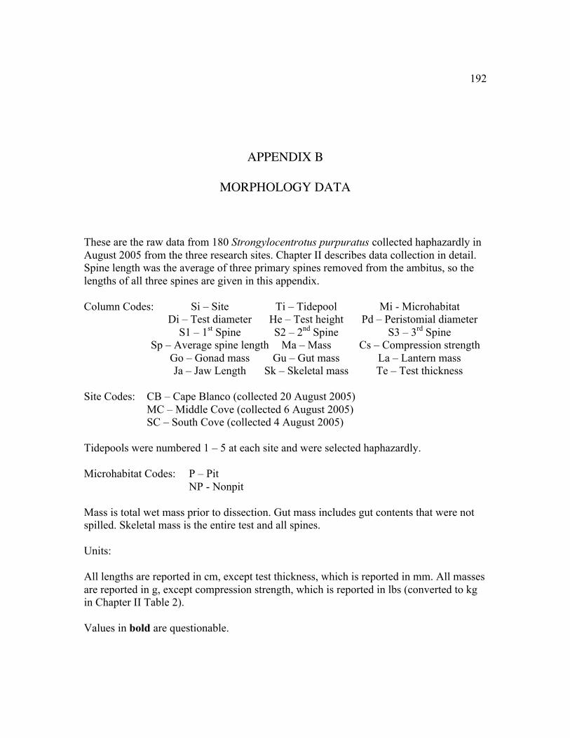
192
APPENDIX B
MORPHOLOGY DATA
These are the raw data from 180 Strongylocentrotus purpuratus collected haphazardly in
August 2005 from the three research sites. Chapter II describes data collection in detail.
Spine length was the average of three primary spines removed from the ambitus, so the
lengths of all three spines are given in this appendix.
Column Codes: Si – Site Ti – Tidepool Mi - Microhabitat
Di – Test diameter He – Test height Pd – Peristomial diameter
S1 – 1st Spine S2 – 2
nd Spine S3 – 3
rd Spine
Sp – Average spine length Ma – Mass Cs – Compression strength
Go – Gonad mass Gu – Gut mass La – Lantern mass
Ja – Jaw Length Sk – Skeletal mass Te – Test thickness
Site Codes: CB – Cape Blanco (collected 20 August 2005)
MC – Middle Cove (collected 6 August 2005)
SC – South Cove (collected 4 August 2005)
Tidepools were numbered 1 – 5 at each site and were selected haphazardly.
Microhabitat Codes: P – Pit
NP - Nonpit
Mass is total wet mass prior to dissection. Gut mass includes gut contents that were not
spilled. Skeletal mass is the entire test and all spines.
Units:
All lengths are reported in cm, except test thickness, which is reported in mm. All masses
are reported in g, except compression strength, which is reported in lbs (converted to kg
in Chapter II Table 2).
Values in bold are questionable.
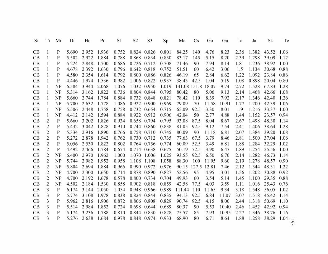
Si Ti Mi Di He Pd S1 S2 S3 Sp Ma Cs Go Gu La Ja Sk Te
CB 1 P 5.690 2.952 1.936 0.752 0.824 0.826 0.801 84.25 140 4.76 8.23 2.36 1.382 43.52 1.06
CB 1 P 5.502 2.922 1.884 0.788 0.868 0.834 0.830 83.17 145 5.15 8.20 2.39 1.298 39.09 1.12
CB 1 P 5.224 2.848 1.700 0.686 0.726 0.712 0.708 71.46 90 7.94 8.14 1.81 1.236 38.92 1.00
CB 1 P 4.678 2.392 1.630 0.796 0.642 0.818 0.752 51.51 60 6.42 3.06 1.5 1.134 30.68 0.88
CB 1 P 4.580 2.354 1.614 0.792 0.800 0.886 0.826 46.19 65 2.84 6.62 1.22 1.092 23.84 0.86
CB 1 P 4.446 1.974 1.536 0.982 1.006 0.822 0.937 38.45 42.5 1.04 5.19 1.08 0.898 20.04 0.80
CB 1 NP 6.584 3.944 2.068 1.076 1.032 0.950 1.019 141.08 151.8 18.07 9.74 2.72 1.528 67.83 1.28
CB 1 NP 5.314 3.162 1.822 0.736 0.804 0.844 0.795 80.42 80 5.06 9.13 2.14 1.468 42.66 1.08
CB 1 NP 5.660 2.744 1.784 0.884 0.732 0.848 0.821 78.42 110 8.39 7.92 2.17 1.346 42.40 1.26
CB 1 NP 5.700 2.632 1.778 1.086 0.922 0.900 0.969 79.09 70 11.58 10.91 1.77 1.200 42.39 1.06
CB 1 NP 5.506 2.448 1.758 0.758 0.732 0.654 0.715 65.09 92.5 3.30 8.01 1.9 1.216 33.37 1.00
CB 1 NP 4.412 2.142 1.594 0.884 0.922 0.912 0.906 42.04 50 2.77 4.88 1.44 1.152 23.57 0.94
CB 2 P 5.660 3.202 1.826 0.934 0.658 0.794 0.795 93.08 87.5 8.04 8.67 2.67 1.498 48.30 1.14
CB 2 P 5.432 3.042 1.828 0.910 0.744 0.860 0.838 81.05 92.5 9.12 7.54 2.41 1.406 38.64 1.28
CB 2 P 5.334 2.916 1.890 0.766 0.758 0.710 0.745 80.09 90 11.18 6.81 2.07 1.384 39.20 1.08
CB 2 P 5.272 2.878 1.942 0.762 0.730 0.712 0.735 77.63 67.5 3.79 8.46 2.81 1.500 37.04 1.06
CB 2 P 5.056 2.530 1.822 0.802 0.764 0.756 0.774 60.09 52.5 3.49 6.81 1.88 1.284 32.29 1.02
CB 2 P 4.492 2.466 1.784 0.674 0.714 0.638 0.675 50.19 72.5 3.90 6.47 1.89 1.254 25.56 1.00
CB 2 NP 6.400 2.970 1.962 1.000 1.070 1.006 1.025 93.55 92.5 6.50 6.70 2.14 1.282 46.73 1.14
CB 2 NP 5.744 2.982 1.952 0.958 1.108 1.108 1.058 88.30 100 11.95 9.60 2.19 1.278 48.57 0.90
CB 2 NP 5.804 2.694 1.884 0.966 0.990 0.972 0.976 90.15 127.5 12.81 7.46 2.12 1.344 48.31 1.22
CB 2 NP 4.700 2.300 1.650 0.714 0.878 0.890 0.827 52.56 95 4.95 3.01 1.56 1.202 30.88 0.92
CB 2 NP 4.700 2.192 1.678 0.578 0.800 0.734 0.704 49.93 60 3.54 5.14 1.45 1.100 29.35 0.88
CB 2 NP 4.502 2.184 1.530 0.858 0.902 0.818 0.859 42.58 77.5 4.03 3.59 1.11 1.016 25.43 0.76
CB 3 P 6.174 3.144 2.050 1.054 0.948 0.966 0.989 111.44 110 11.65 9.34 3.18 1.548 56.05 1.02
CB 3 P 5.774 3.108 1.978 0.838 0.824 0.844 0.835 94.13 92.5 6.84 11.07 3.07 1.518 45.42 1.14
CB 3 P 5.962 2.816 1.906 0.872 0.806 0.808 0.829 90.74 92.5 4.15 8.00 2.44 1.318 50.69 1.10
CB 3 P 5.514 2.984 1.852 0.724 0.698 0.644 0.689 80.37 90 5.53 10.40 2.46 1.452 42.92 0.94
CB 3 P 5.174 3.236 1.788 0.810 0.844 0.830 0.828 75.57 85 7.93 10.95 2.27 1.346 38.76 1.16
CB 3 P 5.276 2.638 1.684 0.978 0.848 0.974 0.933 68.90 80 6.71 8.64 1.88 1.258 38.29 1.04
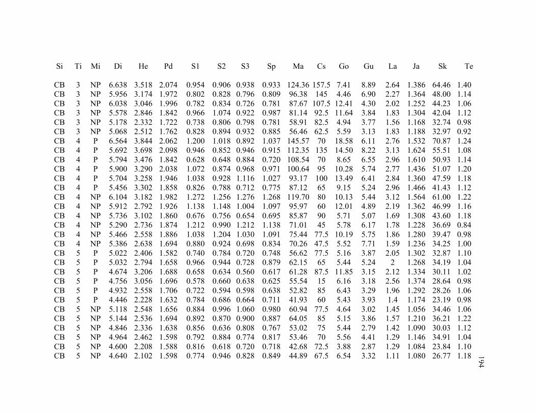
Si Ti Mi Di He Pd S1 S2 S3 Sp Ma Cs Go Gu La Ja Sk Te
CB 3 NP 6.638 3.518 2.074 0.954 0.906 0.938 0.933 124.36 157.5 7.41 8.89 2.64 1.386 64.46 1.40
CB 3 NP 5.956 3.174 1.972 0.802 0.828 0.796 0.809 96.38 145 4.46 6.90 2.27 1.364 48.00 1.14
CB 3 NP 6.038 3.046 1.996 0.782 0.834 0.726 0.781 87.67 107.5 12.41 4.30 2.02 1.252 44.23 1.06
CB 3 NP 5.578 2.846 1.842 0.966 1.074 0.922 0.987 81.14 92.5 11.64 3.84 1.83 1.304 42.04 1.12
CB 3 NP 5.178 2.332 1.722 0.738 0.806 0.798 0.781 58.91 82.5 4.94 3.77 1.56 1.168 32.74 0.98
CB 3 NP 5.068 2.512 1.762 0.828 0.894 0.932 0.885 56.46 62.5 5.59 3.13 1.83 1.188 32.97 0.92
CB 4 P 6.564 3.844 2.062 1.200 1.018 0.892 1.037 145.57 70 18.58 6.11 2.76 1.532 70.87 1.24
CB 4 P 5.692 3.698 2.098 0.946 0.852 0.946 0.915 112.35 135 14.50 8.22 3.13 1.624 55.51 1.08
CB 4 P 5.794 3.476 1.842 0.628 0.648 0.884 0.720 108.54 70 8.65 6.55 2.96 1.610 50.93 1.14
CB 4 P 5.900 3.290 2.038 1.072 0.874 0.968 0.971 100.64 95 10.28 5.74 2.77 1.436 51.07 1.20
CB 4 P 5.704 3.258 1.946 1.038 0.928 1.116 1.027 93.17 100 13.49 6.41 2.84 1.360 47.59 1.18
CB 4 P 5.456 3.302 1.858 0.826 0.788 0.712 0.775 87.12 65 9.15 5.24 2.96 1.466 41.43 1.12
CB 4 NP 6.104 3.182 1.982 1.272 1.256 1.276 1.268 119.70 80 10.13 5.44 3.12 1.564 61.00 1.22
CB 4 NP 5.912 2.792 1.926 1.138 1.148 1.004 1.097 95.97 60 12.01 4.89 2.19 1.362 46.99 1.16
CB 4 NP 5.736 3.102 1.860 0.676 0.756 0.654 0.695 85.87 90 5.71 5.07 1.69 1.308 43.60 1.18
CB 4 NP 5.290 2.736 1.874 1.212 0.990 1.212 1.138 71.01 45 5.78 6.17 1.78 1.228 36.69 0.84
CB 4 NP 5.466 2.558 1.886 1.038 1.204 1.030 1.091 75.44 77.5 10.19 5.75 1.86 1.280 39.47 0.98
CB 4 NP 5.386 2.638 1.694 0.880 0.924 0.698 0.834 70.26 47.5 5.52 7.71 1.59 1.236 34.25 1.00
CB 5 P 5.022 2.406 1.582 0.740 0.784 0.720 0.748 56.62 77.5 5.16 3.87 2.05 1.302 32.87 1.10
CB 5 P 5.032 2.794 1.658 0.966 0.944 0.728 0.879 62.15 65 5.44 5.24 2 1.268 34.19 1.04
CB 5 P 4.674 3.206 1.688 0.658 0.634 0.560 0.617 61.28 87.5 11.85 3.15 2.12 1.334 30.11 1.02
CB 5 P 4.756 3.056 1.696 0.578 0.660 0.638 0.625 55.54 15 6.16 3.18 2.56 1.374 28.64 0.98
CB 5 P 4.932 2.558 1.706 0.722 0.594 0.598 0.638 52.82 85 6.43 3.29 1.96 1.292 28.26 1.06
CB 5 P 4.446 2.228 1.632 0.784 0.686 0.664 0.711 41.93 60 5.43 3.93 1.4 1.174 23.19 0.98
CB 5 NP 5.118 2.548 1.656 0.884 0.996 1.060 0.980 60.94 77.5 4.64 3.02 1.45 1.056 34.46 1.06
CB 5 NP 5.144 2.536 1.694 0.892 0.870 0.900 0.887 64.05 85 5.15 3.86 1.57 1.210 36.21 1.22
CB 5 NP 4.846 2.336 1.638 0.856 0.636 0.808 0.767 53.02 75 5.44 2.79 1.42 1.090 30.03 1.12
CB 5 NP 4.964 2.462 1.598 0.792 0.884 0.774 0.817 53.46 70 5.56 4.41 1.29 1.146 34.91 1.04
CB 5 NP 4.600 2.208 1.588 0.816 0.618 0.720 0.718 42.68 72.5 3.88 2.87 1.29 1.084 23.84 1.10
CB 5 NP 4.640 2.102 1.598 0.774 0.946 0.828 0.849 44.89 67.5 6.54 3.32 1.11 1.080 26.77 1.18
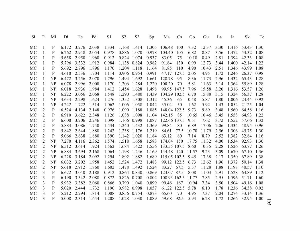
Si Ti Mi Di He Pd S1 S2 S3 Sp Ma Cs Go Gu La Ja Sk Te
MC 1 P 6.172 3.276 2.038 1.334 1.168 1.414 1.305 106.48 100 7.32 12.37 3.30 1.416 53.43 1.30
MC 1 P 6.262 2.948 2.054 0.978 0.886 1.070 0.978 104.40 105 6.82 8.87 3.56 1.472 53.32 1.08
MC 1 P 5.658 2.950 1.960 0.912 0.824 1.074 0.937 83.05 75 10.18 8.49 2.81 1.394 42.33 1.08
MC 1 P 5.796 3.332 1.912 0.984 1.138 0.824 0.982 91.84 130 0.99 12.73 3.44 1.400 42.14 1.22
MC 1 P 5.692 2.796 1.896 1.170 1.204 1.118 1.164 81.85 110 4.90 10.43 2.51 1.346 43.99 1.08
MC 1 P 4.610 2.536 1.704 1.114 0.906 0.954 0.991 47.17 127.5 2.05 4.95 1.72 1.246 26.37 0.98
MC 1 NP 6.472 3.256 2.070 1.796 1.494 1.692 1.661 128.78 95 8.36 11.73 2.96 1.432 65.43 1.28
MC 1 NP 6.078 2.996 2.008 1.170 1.206 1.284 1.220 100.20 70 5.81 11.63 3.14 1.364 55.89 1.28
MC 1 NP 6.018 2.936 1.984 1.412 1.454 1.628 1.498 99.95 147.5 7.96 15.58 3.20 1.316 53.57 1.26
MC 1 NP 6.222 3.056 2.068 1.548 1.290 1.480 1.439 104.29 102.5 6.70 15.88 3.15 1.324 56.37 1.28
MC 1 NP 4.634 2.298 1.624 1.276 1.352 1.308 1.312 45.36 65 0.48 5.87 1.80 1.006 24.44 0.92
MC 1 NP 4.242 1.722 1.514 1.062 1.006 1.058 1.042 35.04 50 1.62 5.92 1.43 1.052 21.25 1.04
MC 2 P 6.524 4.134 2.148 0.976 1.090 1.188 1.085 148.04 122.5 9.73 9.89 3.48 1.560 64.58 1.16
MC 2 P 6.910 3.622 2.348 1.126 1.088 1.098 1.104 142.15 85 10.65 10.46 3.45 1.558 64.93 1.22
MC 2 P 6.600 3.206 2.246 1.098 1.166 0.998 1.087 122.66 137.5 9.51 7.62 3.72 1.552 57.66 1.32
MC 2 P 5.884 3.086 1.740 1.434 1.240 1.432 1.369 99.84 80 6.89 17.06 2.06 1.334 48.95 0.96
MC 2 P 5.842 2.644 1.888 1.242 1.238 1.176 1.219 84.61 77.5 10.70 11.79 2.56 1.306 45.75 1.30
MC 2 P 5.066 2.638 1.880 1.390 1.142 1.020 1.184 63.12 80 7.14 8.79 2.52 1.382 32.84 1.16
MC 2 NP 7.270 4.116 2.362 1.574 1.518 1.658 1.583 174.04 150 17.75 11.32 4.00 1.534 92.93 1.30
MC 2 NP 6.512 3.614 1.924 1.562 1.684 1.422 1.556 133.55 107.5 8.60 10.35 2.28 1.526 63.77 1.26
MC 2 NP 6.884 3.694 2.168 1.064 1.198 1.246 1.169 144.48 120 11.57 9.23 3.09 1.670 67.10 1.36
MC 2 NP 6.228 3.184 2.092 1.294 1.892 1.882 1.689 115.05 102.5 9.45 17.38 2.17 1.350 67.89 1.38
MC 2 NP 6.032 3.202 1.958 1.452 1.524 1.472 1.483 99.12 122.5 6.73 12.62 1.96 1.372 50.14 1.38
MC 2 NP 5.618 2.912 1.860 1.602 1.478 1.492 1.524 83.27 67.5 5.37 11.28 1.88 1.198 40.57 1.10
MC 3 P 6.672 3.040 2.188 0.912 0.864 0.830 0.869 123.07 87.5 8.08 11.03 2.91 1.528 64.89 1.12
MC 3 P 6.190 3.342 2.088 0.872 0.826 0.708 0.802 108.93 162.5 11.77 7.85 2.95 1.596 51.71 1.60
MC 3 P 5.932 3.382 2.060 0.866 0.790 1.040 0.899 99.46 167 10.94 7.34 3.50 1.504 49.16 1.08
MC 3 P 5.020 2.444 1.732 1.190 0.982 0.998 1.057 61.22 122.5 5.78 6.10 1.78 1.236 34.38 0.92
MC 3 P 5.212 2.294 1.814 1.008 0.856 0.754 0.873 65.60 70 4.95 7.37 2.04 1.274 33.14 1.36
MC 3 P 5.008 2.314 1.644 1.208 1.028 1.030 1.089 59.68 92.5 5.93 6.28 1.72 1.266 32.95 1.00
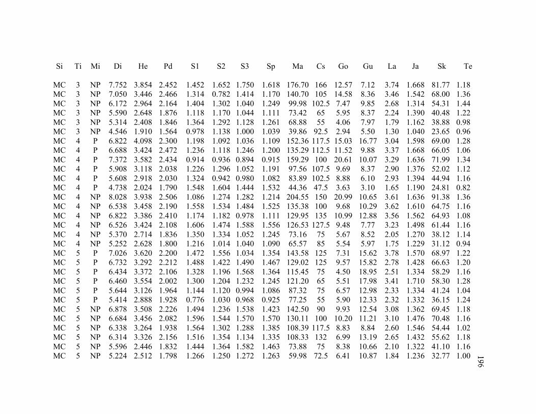
Si Ti Mi Di He Pd S1 S2 S3 Sp Ma Cs Go Gu La Ja Sk Te
MC 3 NP 7.752 3.854 2.452 1.452 1.652 1.750 1.618 176.70 166 12.57 7.12 3.74 1.668 81.77 1.18
MC 3 NP 7.050 3.446 2.466 1.314 0.782 1.414 1.170 140.70 105 14.58 8.36 3.46 1.542 68.00 1.36
MC 3 NP 6.172 2.964 2.164 1.404 1.302 1.040 1.249 99.98 102.5 7.47 9.85 2.68 1.314 54.31 1.44
MC 3 NP 5.590 2.648 1.876 1.118 1.170 1.044 1.111 73.42 65 5.95 8.37 2.24 1.390 40.48 1.22
MC 3 NP 5.314 2.408 1.846 1.364 1.292 1.128 1.261 68.88 55 4.06 7.97 1.79 1.162 38.88 0.98
MC 3 NP 4.546 1.910 1.564 0.978 1.138 1.000 1.039 39.86 92.5 2.94 5.50 1.30 1.040 23.65 0.96
MC 4 P 6.822 4.098 2.300 1.198 1.092 1.036 1.109 152.36 117.5 15.03 16.77 3.04 1.598 69.00 1.28
MC 4 P 6.688 3.424 2.472 1.236 1.118 1.246 1.200 135.29 112.5 11.52 9.88 3.37 1.668 66.05 1.06
MC 4 P 7.372 3.582 2.434 0.914 0.936 0.894 0.915 159.29 100 20.61 10.07 3.29 1.636 71.99 1.34
MC 4 P 5.908 3.118 2.038 1.226 1.296 1.052 1.191 97.56 107.5 9.69 8.37 2.90 1.376 52.02 1.12
MC 4 P 5.608 2.918 2.030 1.324 0.942 0.980 1.082 83.89 102.5 8.88 6.10 2.93 1.394 44.94 1.16
MC 4 P 4.738 2.024 1.790 1.548 1.604 1.444 1.532 44.36 47.5 3.63 3.10 1.65 1.190 24.81 0.82
MC 4 NP 8.028 3.938 2.506 1.086 1.274 1.282 1.214 204.55 150 20.99 10.65 3.61 1.636 91.38 1.36
MC 4 NP 6.538 3.458 2.190 1.558 1.534 1.484 1.525 135.38 100 9.68 10.29 3.62 1.610 64.75 1.16
MC 4 NP 6.822 3.386 2.410 1.174 1.182 0.978 1.111 129.95 135 10.99 12.88 3.56 1.562 64.93 1.08
MC 4 NP 6.526 3.424 2.108 1.606 1.474 1.588 1.556 126.53 127.5 9.48 7.77 3.23 1.498 61.44 1.16
MC 4 NP 5.370 2.714 1.836 1.350 1.334 1.052 1.245 73.16 75 5.67 8.52 2.05 1.270 38.12 1.14
MC 4 NP 5.252 2.628 1.800 1.216 1.014 1.040 1.090 65.57 85 5.54 5.97 1.75 1.229 31.12 0.94
MC 5 P 7.026 3.620 2.200 1.472 1.556 1.034 1.354 143.58 125 7.31 15.62 3.78 1.570 68.97 1.22
MC 5 P 6.732 3.292 2.212 1.488 1.422 1.490 1.467 129.02 125 9.57 15.82 2.78 1.428 66.63 1.20
MC 5 P 6.434 3.372 2.106 1.328 1.196 1.568 1.364 115.45 75 4.50 18.95 2.51 1.334 58.29 1.16
MC 5 P 6.460 3.554 2.002 1.300 1.204 1.232 1.245 121.20 65 5.51 17.98 3.41 1.710 58.30 1.28
MC 5 P 5.644 3.126 1.964 1.144 1.120 0.994 1.086 87.32 75 6.57 12.98 2.33 1.334 41.24 1.04
MC 5 P 5.414 2.888 1.928 0.776 1.030 0.968 0.925 77.25 55 5.90 12.33 2.32 1.332 36.15 1.24
MC 5 NP 6.878 3.508 2.226 1.494 1.236 1.538 1.423 142.50 90 9.93 12.54 3.08 1.362 69.45 1.18
MC 5 NP 6.684 3.456 2.082 1.596 1.544 1.570 1.570 130.11 100 10.20 11.21 3.10 1.476 70.48 1.16
MC 5 NP 6.338 3.264 1.938 1.564 1.302 1.288 1.385 108.39 117.5 8.83 8.84 2.60 1.546 54.44 1.02
MC 5 NP 6.314 3.326 2.156 1.516 1.354 1.134 1.335 108.33 132 6.99 13.19 2.65 1.432 55.62 1.18
MC 5 NP 5.596 2.446 1.832 1.444 1.364 1.582 1.463 73.88 75 8.38 10.66 2.10 1.322 41.10 1.16
MC 5 NP 5.224 2.512 1.798 1.266 1.250 1.272 1.263 59.98 72.5 6.41 10.87 1.84 1.236 32.77 1.00

Si Ti Mi Di He Pd S1 S2 S3 Sp Ma Cs Go Gu La Ja Sk Te
SC 1 P 7.048 3.982 2.294 1.274 0.958 0.988 1.073 159.46 132 11.07 19.29 3.37 1.576 73.77 1.68
SC 1 P 6.168 3.592 2.156 0.768 0.672 0.682 0.707 121.81 115 13.12 10.1 3.3 1.690 56.89 1.24
SC 1 P 5.854 3.450 1.944 1.006 0.828 1.102 0.979 107.99 115 16.54 8.09 2.63 1.368 50.7 1.24
SC 1 P 5.946 3.422 2.098 0.660 0.710 0.698 0.689 105.91 115 7.12 14.88 2.87 1.460 49.41 1.34
SC 1 P 4.978 3.264 1.800 0.778 1.042 0.944 0.921 75.21 82.5 8.12 4.28 2.46 1.348 35.33 0.96
SC 1 P 5.166 2.488 1.746 1.164 0.984 0.762 0.970 63.15 62.5 8.13 5.61 2.12 1.272 31.81 1.14
SC 1 NP 6.836 4.198 2.226 1.042 0.996 1.118 1.052 163.00 120 19.39 6.41 3.67 1.426 81.70 1.50
SC 1 NP 6.220 3.198 2.066 0.780 0.732 0.664 0.725 110.66 112.5 8.25 13.92 2.99 1.478 57.09 1.48
SC 1 NP 6.794 3.766 2.094 0.756 0.688 0.726 0.723 144.72 65 10.70 7.36 3.47 1.364 69.14 1.32
SC 1 NP 4.472 2.256 1.594 0.650 0.766 0.732 0.716 43.66 52.5 2.19 6.30 1.78 1.120 26.30 1.42
SC 1 NP 6.200 3.226 2.158 0.814 0.864 0.908 0.862 110.16 97.5 10.51 15.32 2.78 1.592 65.68 1.20
SC 1 NP 5.242 2.576 1.688 0.820 0.824 0.804 0.816 60.08 52.5 8.98 6.16 2.10 1.128 34.47 1.46
SC 2 P 5.646 2.890 2.020 0.844 0.860 0.638 0.781 77.21 54 8.41 6.35 2.74 1.310 43.18 1.22
SC 2 P 4.938 2.582 1.628 0.728 0.770 0.626 0.708 55.76 64 3.72 5.15 1.24 1.194 30.03 1.08
SC 2 P 5.898 3.282 1.984 1.016 0.912 0.952 0.960 101.29 116 11.52 6.79 2.31 1.356 48.85 1.40
SC 2 P 5.596 3.190 1.910 0.852 1.072 1.000 0.975 94.87 108 7.72 4.92 2.49 1.502 46.17 1.20
SC 2 P 5.764 3.080 1.908 0.834 0.896 0.900 0.877 92.30 70 5.74 9.50 2.57 1.512 47.40 1.60
SC 2 P 6.138 3.226 1.860 0.844 0.872 0.666 0.794 113.19 86 9.02 11.82 2.58 1.492 57.44 1.32
SC 2 NP 6.000 2.910 2.052 0.670 0.862 0.736 0.756 93.97 123 7.89 8.36 2.63 1.278 52.05 1.14
SC 2 NP 7.266 3.796 2.276 0.990 1.024 1.028 1.014 167.86 109 17.53 7.84 3.08 1.606 80.07 1.28
SC 2 NP 6.668 3.392 2.050 1.128 0.976 1.090 1.065 128.30 103 15.47 8.44 3.00 1.592 70.53 1.53
SC 2 NP 6.148 3.370 1.942 0.884 0.990 1.018 0.964 107.66 130 9.81 12.47 2.45 1.466 51.53 1.2
SC 2 NP 5.616 2.858 1.884 0.848 0.876 0.828 0.851 88.66 85 18.39 8.53 2.29 1.338 45.34 1.18
SC 2 NP 5.418 2.802 1.748 0.828 0.856 0.826 0.837 75.32 114 13.11 4.92 2.75 1.388 42.84 1.06
SC 3 P 5.892 2.904 1.876 0.792 0.746 0.690 0.743 88.26 145.5 8.46 8.34 2.44 1.338 48.08 1.52
SC 3 P 6.210 3.362 2.032 0.796 0.938 0.826 0.853 111.87 122.5 20.52 8.35 2.42 1.472 52.02 1.16
SC 3 P 5.658 3.050 1.846 0.884 1.022 0.878 0.928 88.83 100 8.43 6.97 1.82 1.330 42.19 1.10
SC 3 P 6.172 3.302 1.986 0.712 0.764 0.788 0.755 102.33 95 10.27 6.84 2.22 1.314 47.05 1.24
SC 3 P 5.906 3.746 2.010 0.718 0.740 0.788 0.749 105.55 52.5 18.28 13.42 2.36 1.444 52.54 1.28
SC 3 P 4.664 2.190 1.562 0.766 0.800 0.850 0.805 47.30 30 5.36 3.44 1.21 1.140 28.37 1.12
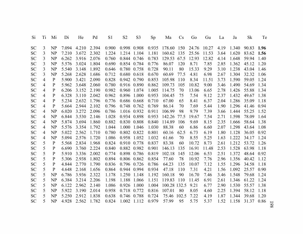
Si Ti Mi Di He Pd S1 S2 S3 Sp Ma Cs Go Gu La Ja Sk Te
SC 3 NP 7.094 4.210 2.394 0.900 0.998 0.908 0.935 178.60 150 24.76 10.27 4.19 1.340 90.83 1.96
SC 3 NP 7.210 3.672 2.302 1.224 1.214 1.104 1.181 160.62 135 25.56 11.53 3.64 1.620 83.62 1.56
SC 3 NP 6.262 3.916 2.076 0.760 0.844 0.746 0.783 129.53 67.5 12.93 12.82 4.14 1.648 59.94 1.40
SC 3 NP 5.576 3.024 1.804 0.690 0.854 0.784 0.776 86.07 120 8.71 7.85 2.85 1.362 45.12 1.20
SC 3 NP 5.540 3.148 1.892 0.646 0.780 0.758 0.728 90.11 80 15.33 9.29 3.10 1.238 43.04 1.46
SC 3 NP 5.268 2.628 1.686 0.712 0.680 0.618 0.670 60.69 77.5 4.81 6.98 2.67 1.304 32.32 1.06
SC 4 P 5.900 3.421 2.090 0.828 0.942 0.790 0.853 105.98 110 8.34 11.51 3.73 1.590 59.05 1.24
SC 4 P 5.962 3.648 2.060 0.780 0.916 0.890 0.862 109.73 105 10.82 9.00 3.46 1.490 54.69 1.34
SC 4 P 6.206 3.152 2.190 0.982 0.960 1.074 1.005 114.75 70 13.06 6.65 2.78 1.426 55.88 1.34
SC 4 P 6.328 3.110 2.042 0.962 0.896 1.000 0.953 104.45 75 7.54 9.12 2.37 1.432 49.67 1.38
SC 4 P 5.234 2.632 1.796 0.776 0.686 0.668 0.710 67.00 65 8.41 6.37 2.04 1.286 35.09 1.18
SC 4 P 5.664 2.944 2.102 0.796 0.748 0.762 0.769 86.14 70 7.69 5.44 1.90 1.296 41.46 0.94
SC 4 NP 6.020 3.272 2.096 0.786 1.016 0.932 0.911 106.99 98 9.79 7.39 3.66 1.444 55.25 1.52
SC 4 NP 6.844 3.530 2.146 1.028 0.934 0.898 0.953 142.26 77.5 19.67 7.54 2.71 1.598 78.09 1.64
SC 4 NP 5.874 3.694 1.860 0.882 0.830 0.808 0.840 114.89 106 9.69 8.15 2.35 1.666 58.64 1.38
SC 4 NP 5.576 3.354 1.792 1.044 1.000 1.046 1.030 88.38 60 6.86 6.60 2.07 1.298 43.64 1.08
SC 4 NP 5.022 2.562 1.710 0.780 0.802 0.822 0.801 60.16 62.5 6.73 6.19 1.80 1.128 36.05 0.92
SC 4 NP 5.094 2.576 1.720 1.086 0.958 1.052 1.032 61.66 70 8.55 5.25 1.63 1.222 34.17 1.24
SC 5 P 5.568 2.834 1.968 0.824 0.910 0.778 0.837 83.38 60 10.72 8.73 2.61 1.212 53.72 1.26
SC 5 P 6.690 3.760 2.224 0.840 0.882 0.982 0.901 146.13 135 16.91 11.48 2.53 1.528 63.98 1.18
SC 5 P 5.910 3.336 2.002 0.774 0.898 0.786 0.819 102.18 145 12.06 6.53 2.51 1.372 48.64 0.92
SC 5 P 5.306 2.938 1.802 0.894 0.806 0.862 0.854 77.60 78 10.92 7.76 2.96 1.356 40.42 1.12
SC 5 P 4.844 2.770 1.790 0.836 0.796 0.726 0.786 64.23 135 10.07 7.12 1.55 1.296 34.58 1.18
SC 5 P 4.648 2.168 1.656 0.864 0.944 0.994 0.934 47.18 110 7.31 4.21 1.56 1.092 25.57 0.90
SC 5 NP 6.786 3.936 2.322 1.178 1.250 1.148 1.192 160.18 90 16.70 7.46 3.46 1.548 79.68 1.24
SC 5 NP 6.384 3.214 2.206 1.198 1.188 1.066 1.151 119.83 110 11.45 6.91 2.61 1.346 61.22 1.24
SC 5 NP 6.122 2.962 2.140 1.086 0.926 1.000 1.004 100.28 132.5 9.21 6.77 2.90 1.530 55.57 1.38
SC 5 NP 5.922 3.190 2.014 0.958 0.718 0.772 0.816 107.01 80 8.05 4.60 2.25 1.394 58.12 1.18
SC 5 NP 5.250 2.912 1.838 0.638 0.746 0.788 0.724 75.46 102.5 7.22 4.19 1.87 1.344 39.68 1.20
SC 5 NP 4.928 2.562 1.782 0.824 1.002 1.112 0.979 57.99 95 5.75 5.37 1.52 1.158 31.37 0.86
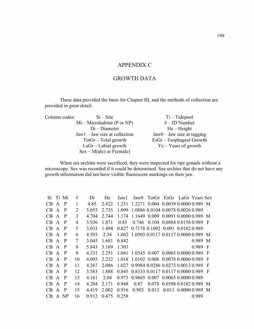
199
APPENDIX C
GROWTH DATA
These data provided the basis for Chapter III, and the methods of collection are
provided in great detail.
Column codes: Si – Site Ti – Tidepool
Mi – Microhabitat (P or NP) # – ID Number
Di – Diameter He – Height
Jaw1 – Jaw size at collection Jaw0 – Jaw size at tagging
TotGr – Total growth EsGr – Esophageal Growth
LaGr – Labial growth Ye – Years of growth
Sex – M(ale) or F(emale)
When sea urchins were sacrificed, they were inspected for ripe gonads without a
microscope. Sex was recorded if it could be determined. Sea urchins that do not have any
growth information did not have visible fluorescent markings on their jaw.
Si Ti Mi # Di He Jaw1 Jaw0 TotGr EsGr LaGr Years Sex
CB A P 1 4.85 2.822 1.231 1.2271 0.004 0.0039 0.0000 0.989 M
CB A P 2 5.055 2.735 1.099 1.0886 0.0104 0.0078 0.0026 0.989
CB A P 3 4.704 2.744 1.174 1.1649 0.009 0.0091 0.0000 0.989 M
CB A P 4 3.936 1.871 0.85 0.746 0.104 0.0884 0.0156 0.989 F
CB A P 5 3.033 1.494 0.827 0.7178 0.1092 0.091 0.0182 0.989
CB A P 6 4.593 2.34 1.062 1.0503 0.0117 0.0117 0.0000 0.989 M
CB A P 7 3.045 1.681 0.842 0.989 M
CB A P 8 5.843 3.169 1.303 0.989 F
CB A P 9 4.331 2.251 1.041 1.0345 0.007 0.0065 0.0000 0.989 F
CB A P 10 4.093 2.232 1.018 1.0102 0.008 0.0078 0.0000 0.989 F
CB A P 11 4.267 2.086 1.027 0.9984 0.0286 0.0273 0.0013 0.989 F
CB A P 12 3.583 1.888 0.845 0.8333 0.0117 0.0117 0.0000 0.989 F
CB A P 13 4.161 2.04 0.973 0.9665 0.007 0.0065 0.0000 0.989
CB A P 14 4.204 2.171 0.948 0.87 0.078 0.0598 0.0182 0.989 M
CB A P 15 4.419 2.002 0.916 0.903 0.013 0.013 0.0000 0.989 M
CB A NP 16 0.912 0.475 0.258 0.989
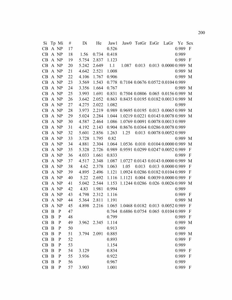
200
Si Tp Mi # Di He Jaw1 Jaw0 TotGr EsGr LaGr Ye Sex
CB A NP 17 0.526 0.989 F
CB A NP 18 1.56 0.734 0.418 0.989
CB A NP 19 5.754 2.837 1.123 0.989 F
CB A NP 20 5.242 2.649 1.1 1.087 0.013 0.013 0.0000 0.989 M
CB A NP 21 4.642 2.521 1.008 0.989 M
CB A NP 22 4.106 1.767 0.906 0.989 M
CB A NP 23 3.569 1.543 0.778 0.7104 0.0676 0.0572 0.0104 0.989
CB A NP 24 3.356 1.664 0.767 0.989 M
CB A NP 25 3.993 1.691 0.831 0.7504 0.0806 0.065 0.0156 0.989 M
CB A NP 26 3.642 2.052 0.863 0.8435 0.0195 0.0182 0.0013 0.989 M
CB A NP 27 4.275 2.022 1.082 0.989
CB A NP 28 3.973 2.219 0.989 0.9695 0.0195 0.013 0.0065 0.989 M
CB A NP 29 5.024 2.284 1.044 1.0219 0.0221 0.0143 0.0078 0.989 M
CB A NP 30 4.587 2.464 1.086 1.0769 0.0091 0.0078 0.0013 0.989
CB A NP 31 4.192 2.143 0.904 0.8676 0.0364 0.0286 0.0078 0.989
CB A NP 32 5.601 2.856 1.263 1.25 0.013 0.0078 0.0052 0.989
CB A NP 33 3.728 1.795 0.82 0.989 M
CB A NP 34 4.881 2.304 1.064 1.0536 0.010 0.0104 0.0000 0.989 M
CB A NP 35 5.328 2.726 0.989 0.9591 0.0299 0.0247 0.0052 0.989 F
CB A NP 36 4.033 1.661 0.833 0.989 F
CB A NP 37 4.517 2.348 1.087 1.0727 0.0143 0.0143 0.0000 0.989 M
CB A NP 38 4.62 2.378 1.063 1.05 0.013 0.013 0.0000 0.989 F
CB A NP 39 4.895 2.496 1.121 1.0924 0.0286 0.0182 0.0104 0.989 F
CB A NP 40 5.22 2.692 1.116 1.1121 0.004 0.0039 0.0000 0.989 F
CB A NP 41 5.042 2.544 1.153 1.1244 0.0286 0.026 0.0026 0.989 M
CB A NP 42 4.83 1.981 0.994 0.989
CB A NP 43 4.798 2.312 1.116 0.989 F
CB A NP 44 5.364 2.811 1.191 0.989 M
CB A NP 45 4.898 2.216 1.065 1.0468 0.0182 0.013 0.0052 0.989 F
CB B P 47 0.764 0.6886 0.0754 0.065 0.0104 0.989 F
CB B P 48 0.799 0.989 F
CB B P 49 3.962 2.345 1.114 0.989 M
CB B P 50 0.913 0.989
CB B P 51 3.794 2.091 0.885 0.989 M
CB B P 52 0.893 0.989 F
CB B P 53 1.154 0.989
CB B P 54 3.129 0.834 0.989 F
CB B P 55 3.936 0.922 0.989 F
CB B P 56 0.967 0.989
CB B P 57 3.903 1.001 0.989 F
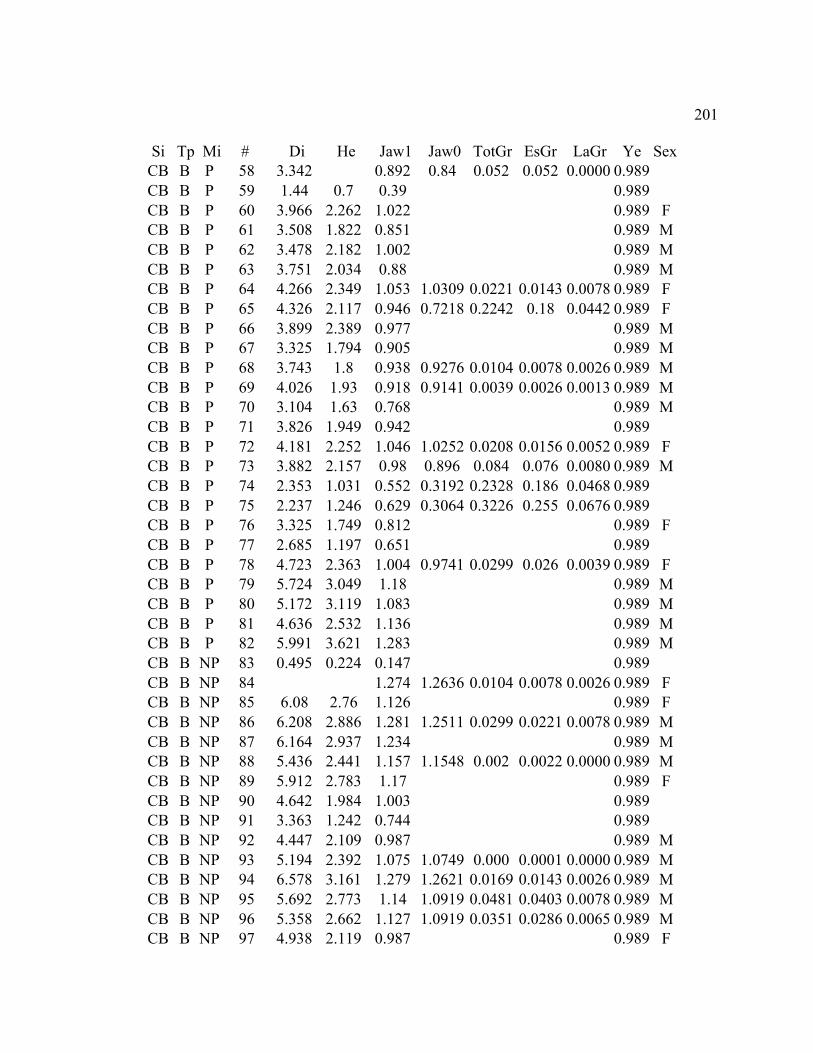
201
Si Tp Mi # Di He Jaw1 Jaw0 TotGr EsGr LaGr Ye Sex
CB B P 58 3.342 0.892 0.84 0.052 0.052 0.0000 0.989
CB B P 59 1.44 0.7 0.39 0.989
CB B P 60 3.966 2.262 1.022 0.989 F
CB B P 61 3.508 1.822 0.851 0.989 M
CB B P 62 3.478 2.182 1.002 0.989 M
CB B P 63 3.751 2.034 0.88 0.989 M
CB B P 64 4.266 2.349 1.053 1.0309 0.0221 0.0143 0.0078 0.989 F
CB B P 65 4.326 2.117 0.946 0.7218 0.2242 0.18 0.0442 0.989 F
CB B P 66 3.899 2.389 0.977 0.989 M
CB B P 67 3.325 1.794 0.905 0.989 M
CB B P 68 3.743 1.8 0.938 0.9276 0.0104 0.0078 0.0026 0.989 M
CB B P 69 4.026 1.93 0.918 0.9141 0.0039 0.0026 0.0013 0.989 M
CB B P 70 3.104 1.63 0.768 0.989 M
CB B P 71 3.826 1.949 0.942 0.989
CB B P 72 4.181 2.252 1.046 1.0252 0.0208 0.0156 0.0052 0.989 F
CB B P 73 3.882 2.157 0.98 0.896 0.084 0.076 0.0080 0.989 M
CB B P 74 2.353 1.031 0.552 0.3192 0.2328 0.186 0.0468 0.989
CB B P 75 2.237 1.246 0.629 0.3064 0.3226 0.255 0.0676 0.989
CB B P 76 3.325 1.749 0.812 0.989 F
CB B P 77 2.685 1.197 0.651 0.989
CB B P 78 4.723 2.363 1.004 0.9741 0.0299 0.026 0.0039 0.989 F
CB B P 79 5.724 3.049 1.18 0.989 M
CB B P 80 5.172 3.119 1.083 0.989 M
CB B P 81 4.636 2.532 1.136 0.989 M
CB B P 82 5.991 3.621 1.283 0.989 M
CB B NP 83 0.495 0.224 0.147 0.989
CB B NP 84 1.274 1.2636 0.0104 0.0078 0.0026 0.989 F
CB B NP 85 6.08 2.76 1.126 0.989 F
CB B NP 86 6.208 2.886 1.281 1.2511 0.0299 0.0221 0.0078 0.989 M
CB B NP 87 6.164 2.937 1.234 0.989 M
CB B NP 88 5.436 2.441 1.157 1.1548 0.002 0.0022 0.0000 0.989 M
CB B NP 89 5.912 2.783 1.17 0.989 F
CB B NP 90 4.642 1.984 1.003 0.989
CB B NP 91 3.363 1.242 0.744 0.989
CB B NP 92 4.447 2.109 0.987 0.989 M
CB B NP 93 5.194 2.392 1.075 1.0749 0.000 0.0001 0.0000 0.989 M
CB B NP 94 6.578 3.161 1.279 1.2621 0.0169 0.0143 0.0026 0.989 M
CB B NP 95 5.692 2.773 1.14 1.0919 0.0481 0.0403 0.0078 0.989 M
CB B NP 96 5.358 2.662 1.127 1.0919 0.0351 0.0286 0.0065 0.989 M
CB B NP 97 4.938 2.119 0.987 0.989 F
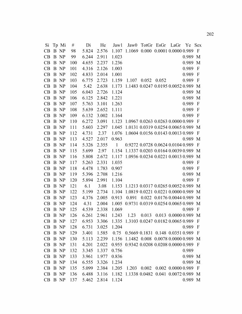
202
Si Tp Mi # Di He Jaw1 Jaw0 TotGr EsGr LaGr Ye Sex
CB B NP 98 5.824 2.576 1.107 1.1069 0.000 0.0001 0.0000 0.989 F
CB B NP 99 6.244 2.911 1.023 0.989 M
CB B NP 100 4.655 2.237 1.236 0.989 M
CB B NP 101 4.316 2.126 1.003 0.989 F
CB B NP 102 4.833 2.014 1.001 0.989 F
CB B NP 103 6.775 2.723 1.159 1.107 0.052 0.052 0.989 F
CB B NP 104 5.42 2.638 1.173 1.1483 0.0247 0.0195 0.0052 0.989 M
CB B NP 105 6.043 2.726 1.124 0.989 M
CB B NP 106 6.125 2.842 1.221 0.989 M
CB B NP 107 5.763 3.101 1.263 0.989 F
CB B NP 108 5.639 2.652 1.111 0.989 F
CB B NP 109 6.132 3.002 1.164 0.989 F
CB B NP 110 6.272 3.091 1.123 1.0967 0.0263 0.0263 0.0000 0.989 F
CB B NP 111 5.603 2.297 1.045 1.0131 0.0319 0.0254 0.0065 0.989 M
CB B NP 112 4.731 2.37 1.076 1.0604 0.0156 0.0143 0.0013 0.989 F
CB B NP 113 4.527 2.017 0.963 0.989 M
CB B NP 114 5.326 2.355 1 0.9272 0.0728 0.0624 0.0104 0.989 F
CB B NP 115 5.699 2.97 1.154 1.1337 0.0203 0.0164 0.0039 0.989 M
CB B NP 116 5.808 2.672 1.117 1.0936 0.0234 0.0221 0.0013 0.989 M
CB B NP 117 5.263 2.331 1.035 0.989 F
CB B NP 118 4.478 1.783 0.907 0.989 F
CB B NP 119 5.396 2.708 1.216 0.989 M
CB B NP 120 5.894 2.991 1.104 0.989 F
CB B NP 121 6.1 3.08 1.153 1.1213 0.0317 0.0265 0.0052 0.989 M
CB B NP 122 5.199 2.734 1.104 1.0819 0.0221 0.0221 0.0000 0.989 M
CB B NP 123 4.376 2.005 0.913 0.891 0.022 0.0176 0.0044 0.989 M
CB B NP 124 4.31 2.004 1.005 0.9731 0.0319 0.0254 0.0065 0.989 M
CB B NP 125 4.539 2.338 1.069 0.989 F
CB B NP 126 6.261 2.961 1.243 1.23 0.013 0.013 0.0000 0.989 M
CB B NP 127 6.953 3.306 1.335 1.3103 0.0247 0.0182 0.0065 0.989 F
CB B NP 128 6.731 3.025 1.204 0.989 F
CB B NP 129 3.401 1.585 0.75 0.5669 0.1831 0.148 0.0351 0.989 F
CB B NP 130 5.113 2.239 1.156 1.1482 0.008 0.0078 0.0000 0.989 M
CB B NP 131 4.201 2.022 0.955 0.9342 0.0208 0.0208 0.0000 0.989 F
CB B NP 132 3.345 1.337 0.756 0.989
CB B NP 133 3.961 1.977 0.836 0.989 M
CB B NP 134 6.555 3.326 1.234 0.989 M
CB B NP 135 5.099 2.384 1.205 1.203 0.002 0.002 0.0000 0.989 F
CB B NP 136 6.488 3.116 1.182 1.1338 0.0482 0.041 0.0072 0.989 M
CB B NP 137 5.462 2.814 1.124 0.989 M

203
Si Tp Mi # Di He Jaw1 Jaw0 TotGr EsGr LaGr Ye Sex
CB B NP 138 5.341 2.548 1.057 0.989 M
CB B NP 139 4.182 2.208 1.006 0.9787 0.0273 0.0247 0.0026 0.989 M
CB B NP 140 5.609 2.62 1.08 1.0464 0.0336 0.0286 0.0050 0.989 M
CB B NP 141 5.27 2.242 1.079 0.989 F
CB B NP 142 5.748 3.183 1.065 1.0494 0.0156 0.0143 0.0013 0.989 M
CB B NP 143 4.434 2.345 1.049 1.0427 0.006 0.0063 0.0000 0.989 M
CB B NP 144 4.087 1.984 0.943 0.989
CB B NP 145 4.69 2.273 1.11 0.989 M
CB B NP 146 4.864 2.152 1.024 0.989 F
CB B NP 147 6.397 3.342 1.284 1.2773 0.007 0.0067 0.0000 0.989 M
CB B NP 148 6.269 2.521 1.239 1.2356 0.003 0.0034 0.0000 0.989 M
CB B NP 149 4.259 1.849 0.932 0.989 M
CB B NP 150 5.637 2.39 1.009 0.989 F
CB B NP 151 5.224 2.483 1.108 1.0472 0.0608 0.0574 0.0034 0.989 M
CB B NP 152 4.691 2.022 1.051 0.989 M
CB B NP 153 7.275 3.651 1.422 1.4051 0.0169 0.0169 0.0000 0.989 M
CB B NP 154 4.421 2.442 1.044 0.989
CB B NP 155 5.562 2.861 1.234 1.2158 0.0182 0.0182 0.0000 0.989
CB B NP 156 6.557 3.193 1.298 0.989
CB C P 900 0.882 1.066
CB C P 901 4.841 2.826 1.149 1.066
CB C P 902 3.817 1.782 0.865 0.6412 0.2238 0.177 0.0468 1.066
CB C P 903 4.386 2.716 1.143 1.066 M
CB C P 904 3.86 1.927 0.879 1.066
CB C P 905 4.538 2.741 1.1 1.0948 0.005 0.0052 0.0000 1.066 M
CB C P 906 5.192 2.862 1.199 1.1834 0.0156 0.0104 0.0052 1.066 F
CB C P 907 5.567 2.988 1.089 1.076 0.013 0.0091 0.0039 1.066 F
CB C P 908 4.928 2.737 1.134 1.1275 0.007 0.0065 0.0000 1.066
CB C P 909 4.25 2.191 1.012 0.9912 0.0208 0.0156 0.0052 1.066
CB C P 910 3.948 2.077 0.916 0.8653 0.0507 0.0416 0.0091 1.066
CB C P 911 4.565 2.154 0.982 0.9716 0.010 0.0104 0.0000 1.066
CB C P 912 5.447 3.116 1.218 1.2102 0.008 0.0078 0.0000 1.066
CB C P 913 4.424 2.299 1.021 0.9612 0.0598 0.052 0.0078 1.066 M
CB C P 914 4.713 2.262 0.992 1.066 M
CB C P 915 4.076 2.196 0.963 1.066
CB C P 916 4.096 2.144 0.881 1.066
CB C P 917 4.655 2.332 0.957 0.9037 0.0533 0.0429 0.0104 1.066
CB C P 918 5.548 2.806 1.066 1.0283 0.0377 0.0325 0.0052 1.066 F
CB C P 919 3.145 1.39 0.719 1.066
CB C P 920 4.03 2.119 0.964 1.066
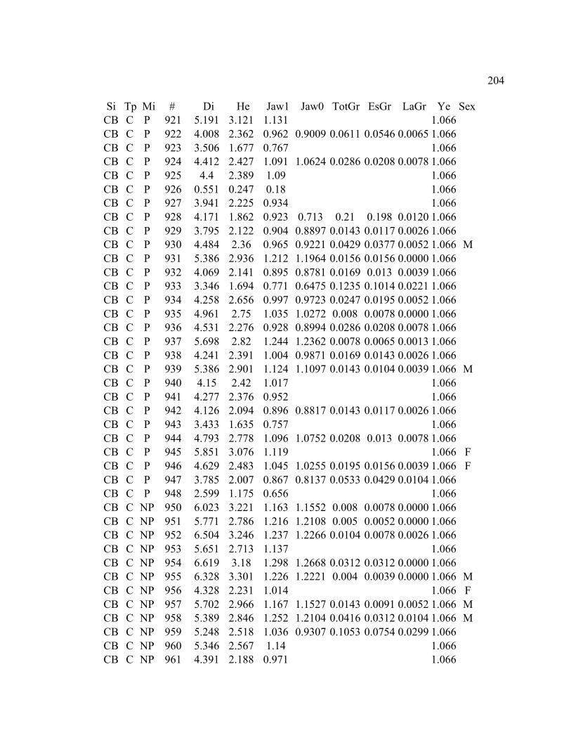
204
Si Tp Mi # Di He Jaw1 Jaw0 TotGr EsGr LaGr Ye Sex
CB C P 921 5.191 3.121 1.131 1.066
CB C P 922 4.008 2.362 0.962 0.9009 0.0611 0.0546 0.0065 1.066
CB C P 923 3.506 1.677 0.767 1.066
CB C P 924 4.412 2.427 1.091 1.0624 0.0286 0.0208 0.0078 1.066
CB C P 925 4.4 2.389 1.09 1.066
CB C P 926 0.551 0.247 0.18 1.066
CB C P 927 3.941 2.225 0.934 1.066
CB C P 928 4.171 1.862 0.923 0.713 0.21 0.198 0.0120 1.066
CB C P 929 3.795 2.122 0.904 0.8897 0.0143 0.0117 0.0026 1.066
CB C P 930 4.484 2.36 0.965 0.9221 0.0429 0.0377 0.0052 1.066 M
CB C P 931 5.386 2.936 1.212 1.1964 0.0156 0.0156 0.0000 1.066
CB C P 932 4.069 2.141 0.895 0.8781 0.0169 0.013 0.0039 1.066
CB C P 933 3.346 1.694 0.771 0.6475 0.1235 0.1014 0.0221 1.066
CB C P 934 4.258 2.656 0.997 0.9723 0.0247 0.0195 0.0052 1.066
CB C P 935 4.961 2.75 1.035 1.0272 0.008 0.0078 0.0000 1.066
CB C P 936 4.531 2.276 0.928 0.8994 0.0286 0.0208 0.0078 1.066
CB C P 937 5.698 2.82 1.244 1.2362 0.0078 0.0065 0.0013 1.066
CB C P 938 4.241 2.391 1.004 0.9871 0.0169 0.0143 0.0026 1.066
CB C P 939 5.386 2.901 1.124 1.1097 0.0143 0.0104 0.0039 1.066 M
CB C P 940 4.15 2.42 1.017 1.066
CB C P 941 4.277 2.376 0.952 1.066
CB C P 942 4.126 2.094 0.896 0.8817 0.0143 0.0117 0.0026 1.066
CB C P 943 3.433 1.635 0.757 1.066
CB C P 944 4.793 2.778 1.096 1.0752 0.0208 0.013 0.0078 1.066
CB C P 945 5.851 3.076 1.119 1.066 F
CB C P 946 4.629 2.483 1.045 1.0255 0.0195 0.0156 0.0039 1.066 F
CB C P 947 3.785 2.007 0.867 0.8137 0.0533 0.0429 0.0104 1.066
CB C P 948 2.599 1.175 0.656 1.066
CB C NP 950 6.023 3.221 1.163 1.1552 0.008 0.0078 0.0000 1.066
CB C NP 951 5.771 2.786 1.216 1.2108 0.005 0.0052 0.0000 1.066
CB C NP 952 6.504 3.246 1.237 1.2266 0.0104 0.0078 0.0026 1.066
CB C NP 953 5.651 2.713 1.137 1.066
CB C NP 954 6.619 3.18 1.298 1.2668 0.0312 0.0312 0.0000 1.066
CB C NP 955 6.328 3.301 1.226 1.2221 0.004 0.0039 0.0000 1.066 M
CB C NP 956 4.328 2.231 1.014 1.066 F
CB C NP 957 5.702 2.966 1.167 1.1527 0.0143 0.0091 0.0052 1.066 M
CB C NP 958 5.389 2.846 1.252 1.2104 0.0416 0.0312 0.0104 1.066 M
CB C NP 959 5.248 2.518 1.036 0.9307 0.1053 0.0754 0.0299 1.066
CB C NP 960 5.346 2.567 1.14 1.066
CB C NP 961 4.391 2.188 0.971 1.066
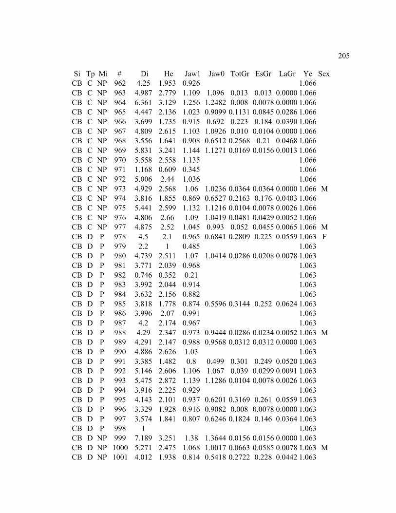
205
Si Tp Mi # Di He Jaw1 Jaw0 TotGr EsGr LaGr Ye Sex
CB C NP 962 4.25 1.953 0.926 1.066
CB C NP 963 4.987 2.779 1.109 1.096 0.013 0.013 0.0000 1.066
CB C NP 964 6.361 3.129 1.256 1.2482 0.008 0.0078 0.0000 1.066
CB C NP 965 4.447 2.136 1.023 0.9099 0.1131 0.0845 0.0286 1.066
CB C NP 966 3.699 1.735 0.915 0.692 0.223 0.184 0.0390 1.066
CB C NP 967 4.809 2.615 1.103 1.0926 0.010 0.0104 0.0000 1.066
CB C NP 968 3.556 1.641 0.908 0.6512 0.2568 0.21 0.0468 1.066
CB C NP 969 5.831 3.241 1.144 1.1271 0.0169 0.0156 0.0013 1.066
CB C NP 970 5.558 2.558 1.135 1.066
CB C NP 971 1.168 0.609 0.345 1.066
CB C NP 972 5.006 2.44 1.036 1.066
CB C NP 973 4.929 2.568 1.06 1.0236 0.0364 0.0364 0.0000 1.066 M
CB C NP 974 3.816 1.855 0.869 0.6527 0.2163 0.176 0.0403 1.066
CB C NP 975 5.441 2.599 1.132 1.1216 0.0104 0.0078 0.0026 1.066
CB C NP 976 4.806 2.66 1.09 1.0419 0.0481 0.0429 0.0052 1.066
CB C NP 977 4.875 2.52 1.045 0.993 0.052 0.0455 0.0065 1.066 M
CB D P 978 4.5 2.1 0.965 0.6841 0.2809 0.225 0.0559 1.063 F
CB D P 979 2.2 1 0.485 1.063
CB D P 980 4.739 2.511 1.07 1.0414 0.0286 0.0208 0.0078 1.063
CB D P 981 3.771 2.039 0.968 1.063
CB D P 982 0.746 0.352 0.21 1.063
CB D P 983 3.992 2.044 0.914 1.063
CB D P 984 3.632 2.156 0.882 1.063
CB D P 985 3.818 1.778 0.874 0.5596 0.3144 0.252 0.0624 1.063
CB D P 986 3.996 2.07 0.991 1.063
CB D P 987 4.2 2.174 0.967 1.063
CB D P 988 4.29 2.347 0.973 0.9444 0.0286 0.0234 0.0052 1.063 M
CB D P 989 4.291 2.147 0.988 0.9568 0.0312 0.0312 0.0000 1.063
CB D P 990 4.886 2.626 1.03 1.063
CB D P 991 3.385 1.482 0.8 0.499 0.301 0.249 0.0520 1.063
CB D P 992 5.146 2.606 1.106 1.067 0.039 0.0299 0.0091 1.063
CB D P 993 5.475 2.872 1.139 1.1286 0.0104 0.0078 0.0026 1.063
CB D P 994 3.916 2.225 0.929 1.063
CB D P 995 4.143 2.101 0.937 0.6201 0.3169 0.261 0.0559 1.063
CB D P 996 3.329 1.928 0.916 0.9082 0.008 0.0078 0.0000 1.063
CB D P 997 3.574 1.841 0.807 0.6246 0.1824 0.146 0.0364 1.063
CB D P 998 1 1.063
CB D NP 999 7.189 3.251 1.38 1.3644 0.0156 0.0156 0.0000 1.063
CB D NP 1000 5.271 2.475 1.068 1.0017 0.0663 0.0585 0.0078 1.063 M
CB D NP 1001 4.012 1.938 0.814 0.5418 0.2722 0.228 0.0442 1.063
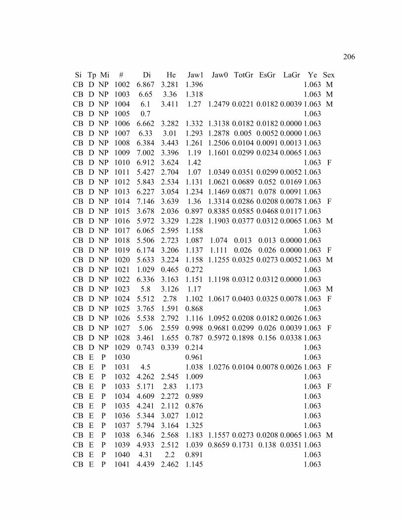
206
Si Tp Mi # Di He Jaw1 Jaw0 TotGr EsGr LaGr Ye Sex
CB D NP 1002 6.867 3.281 1.396 1.063 M
CB D NP 1003 6.65 3.36 1.318 1.063 M
CB D NP 1004 6.1 3.411 1.27 1.2479 0.0221 0.0182 0.0039 1.063 M
CB D NP 1005 0.7 1.063
CB D NP 1006 6.662 3.282 1.332 1.3138 0.0182 0.0182 0.0000 1.063
CB D NP 1007 6.33 3.01 1.293 1.2878 0.005 0.0052 0.0000 1.063
CB D NP 1008 6.384 3.443 1.261 1.2506 0.0104 0.0091 0.0013 1.063
CB D NP 1009 7.002 3.396 1.19 1.1601 0.0299 0.0234 0.0065 1.063
CB D NP 1010 6.912 3.624 1.42 1.063 F
CB D NP 1011 5.427 2.704 1.07 1.0349 0.0351 0.0299 0.0052 1.063
CB D NP 1012 5.843 2.534 1.131 1.0621 0.0689 0.052 0.0169 1.063
CB D NP 1013 6.227 3.054 1.234 1.1469 0.0871 0.078 0.0091 1.063
CB D NP 1014 7.146 3.639 1.36 1.3314 0.0286 0.0208 0.0078 1.063 F
CB D NP 1015 3.678 2.036 0.897 0.8385 0.0585 0.0468 0.0117 1.063
CB D NP 1016 5.972 3.329 1.228 1.1903 0.0377 0.0312 0.0065 1.063 M
CB D NP 1017 6.065 2.595 1.158 1.063
CB D NP 1018 5.506 2.723 1.087 1.074 0.013 0.013 0.0000 1.063
CB D NP 1019 6.174 3.206 1.137 1.111 0.026 0.026 0.0000 1.063 F
CB D NP 1020 5.633 3.224 1.158 1.1255 0.0325 0.0273 0.0052 1.063 M
CB D NP 1021 1.029 0.465 0.272 1.063
CB D NP 1022 6.336 3.163 1.151 1.1198 0.0312 0.0312 0.0000 1.063
CB D NP 1023 5.8 3.126 1.17 1.063 M
CB D NP 1024 5.512 2.78 1.102 1.0617 0.0403 0.0325 0.0078 1.063 F
CB D NP 1025 3.765 1.591 0.868 1.063
CB D NP 1026 5.538 2.792 1.116 1.0952 0.0208 0.0182 0.0026 1.063
CB D NP 1027 5.06 2.559 0.998 0.9681 0.0299 0.026 0.0039 1.063 F
CB D NP 1028 3.461 1.655 0.787 0.5972 0.1898 0.156 0.0338 1.063
CB D NP 1029 0.743 0.339 0.214 1.063
CB E P 1030 0.961 1.063
CB E P 1031 4.5 1.038 1.0276 0.0104 0.0078 0.0026 1.063 F
CB E P 1032 4.262 2.545 1.009 1.063
CB E P 1033 5.171 2.83 1.173 1.063 F
CB E P 1034 4.609 2.272 0.989 1.063
CB E P 1035 4.241 2.112 0.876 1.063
CB E P 1036 5.344 3.027 1.012 1.063
CB E P 1037 5.794 3.164 1.325 1.063
CB E P 1038 6.346 2.568 1.183 1.1557 0.0273 0.0208 0.0065 1.063 M
CB E P 1039 4.933 2.512 1.039 0.8659 0.1731 0.138 0.0351 1.063
CB E P 1040 4.31 2.2 0.891 1.063
CB E P 1041 4.439 2.462 1.145 1.063
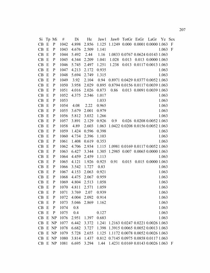
207
Si Tp Mi # Di He Jaw1 Jaw0 TotGr EsGr LaGr Ye Sex
CB E P 1042 4.898 2.856 1.125 1.1249 0.000 0.0001 0.0000 1.063 F
CB E P 1043 4.676 2.509 1.141 1.063 F
CB E P 1044 5.492 2.44 1.16 1.0833 0.0767 0.0624 0.0143 1.063
CB E P 1045 4.344 2.209 1.041 1.028 0.013 0.013 0.0000 1.063
CB E P 1046 5.745 2.497 1.251 1.238 0.013 0.0117 0.0013 1.063
CB E P 1047 4.213 2.172 0.935 1.063
CB E P 1048 5.694 2.749 1.315 1.063
CB E P 1049 3.92 2.104 0.94 0.8971 0.0429 0.0377 0.0052 1.063
CB E P 1050 3.958 2.029 0.895 0.8794 0.0156 0.0117 0.0039 1.063
CB E P 1051 4.016 2.026 0.873 0.86 0.013 0.0091 0.0039 1.063
CB E P 1052 4.375 2.546 1.017 1.063
CB E P 1053 1.033 1.063
CB E P 1054 4.08 2.22 0.965 1.063
CB E P 1055 3.679 2.001 0.979 1.063
CB E P 1056 5.812 3.032 1.266 1.063
CB E P 1057 3.891 2.129 0.926 0.9 0.026 0.0208 0.0052 1.063
CB E P 1058 4.89 2.603 1.063 1.0422 0.0208 0.0156 0.0052 1.063
CB E P 1059 1.424 0.596 0.398 1.063
CB E P 1060 4.734 2.396 1.103 1.063
CB E P 1061 1.408 0.619 0.353 1.063
CB E P 1062 4.706 2.934 1.115 1.0981 0.0169 0.0117 0.0052 1.063
CB E P 1063 6.427 3.344 1.305 1.2985 0.007 0.0065 0.0000 1.063
CB E P 1064 4.459 2.459 1.113 1.063
CB E P 1065 4.121 1.926 0.925 0.91 0.015 0.015 0.0000 1.063
CB E P 1066 3.542 1.727 0.83 1.063
CB E P 1067 4.153 2.063 0.921 1.063
CB E P 1068 4.475 2.067 0.959 1.063
CB E P 1069 4.804 2.513 1.058 1.063
CB E P 1070 4.811 2.571 1.059 1.063
CB E P 1071 3.769 2.07 0.939 1.063
CB E P 1072 4.004 2.092 0.914 1.063
CB E P 1073 5.046 2.869 1.162 1.063
CB E P 1074 0.8 1.063
CB E P 1075 0.4 0.127 1.063
CB E NP 1076 2.951 1.397 0.683 1.063
CB E NP 1077 6.442 3.372 1.241 1.2163 0.0247 0.0221 0.0026 1.063
CB E NP 1078 6.682 3.727 1.398 1.3915 0.0065 0.0052 0.0013 1.063
CB E NP 1079 5.728 2.655 1.125 1.1172 0.0078 0.0052 0.0026 1.063
CB E NP 1080 3.814 1.437 0.812 0.7145 0.0975 0.0858 0.0117 1.063
CB E NP 1081 6.695 3.294 1.44 1.4231 0.0169 0.0143 0.0026 1.063 F
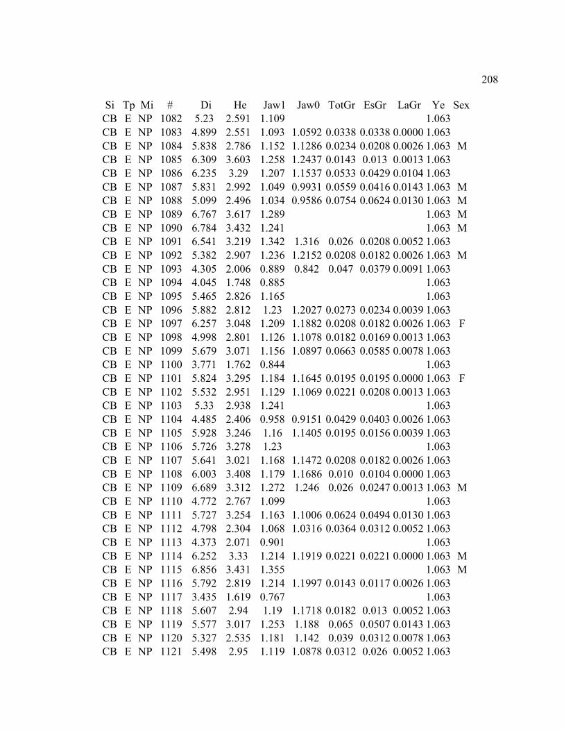
208
Si Tp Mi # Di He Jaw1 Jaw0 TotGr EsGr LaGr Ye Sex
CB E NP 1082 5.23 2.591 1.109 1.063
CB E NP 1083 4.899 2.551 1.093 1.0592 0.0338 0.0338 0.0000 1.063
CB E NP 1084 5.838 2.786 1.152 1.1286 0.0234 0.0208 0.0026 1.063 M
CB E NP 1085 6.309 3.603 1.258 1.2437 0.0143 0.013 0.0013 1.063
CB E NP 1086 6.235 3.29 1.207 1.1537 0.0533 0.0429 0.0104 1.063
CB E NP 1087 5.831 2.992 1.049 0.9931 0.0559 0.0416 0.0143 1.063 M
CB E NP 1088 5.099 2.496 1.034 0.9586 0.0754 0.0624 0.0130 1.063 M
CB E NP 1089 6.767 3.617 1.289 1.063 M
CB E NP 1090 6.784 3.432 1.241 1.063 M
CB E NP 1091 6.541 3.219 1.342 1.316 0.026 0.0208 0.0052 1.063
CB E NP 1092 5.382 2.907 1.236 1.2152 0.0208 0.0182 0.0026 1.063 M
CB E NP 1093 4.305 2.006 0.889 0.842 0.047 0.0379 0.0091 1.063
CB E NP 1094 4.045 1.748 0.885 1.063
CB E NP 1095 5.465 2.826 1.165 1.063
CB E NP 1096 5.882 2.812 1.23 1.2027 0.0273 0.0234 0.0039 1.063
CB E NP 1097 6.257 3.048 1.209 1.1882 0.0208 0.0182 0.0026 1.063 F
CB E NP 1098 4.998 2.801 1.126 1.1078 0.0182 0.0169 0.0013 1.063
CB E NP 1099 5.679 3.071 1.156 1.0897 0.0663 0.0585 0.0078 1.063
CB E NP 1100 3.771 1.762 0.844 1.063
CB E NP 1101 5.824 3.295 1.184 1.1645 0.0195 0.0195 0.0000 1.063 F
CB E NP 1102 5.532 2.951 1.129 1.1069 0.0221 0.0208 0.0013 1.063
CB E NP 1103 5.33 2.938 1.241 1.063
CB E NP 1104 4.485 2.406 0.958 0.9151 0.0429 0.0403 0.0026 1.063
CB E NP 1105 5.928 3.246 1.16 1.1405 0.0195 0.0156 0.0039 1.063
CB E NP 1106 5.726 3.278 1.23 1.063
CB E NP 1107 5.641 3.021 1.168 1.1472 0.0208 0.0182 0.0026 1.063
CB E NP 1108 6.003 3.408 1.179 1.1686 0.010 0.0104 0.0000 1.063
CB E NP 1109 6.689 3.312 1.272 1.246 0.026 0.0247 0.0013 1.063 M
CB E NP 1110 4.772 2.767 1.099 1.063
CB E NP 1111 5.727 3.254 1.163 1.1006 0.0624 0.0494 0.0130 1.063
CB E NP 1112 4.798 2.304 1.068 1.0316 0.0364 0.0312 0.0052 1.063
CB E NP 1113 4.373 2.071 0.901 1.063
CB E NP 1114 6.252 3.33 1.214 1.1919 0.0221 0.0221 0.0000 1.063 M
CB E NP 1115 6.856 3.431 1.355 1.063 M
CB E NP 1116 5.792 2.819 1.214 1.1997 0.0143 0.0117 0.0026 1.063
CB E NP 1117 3.435 1.619 0.767 1.063
CB E NP 1118 5.607 2.94 1.19 1.1718 0.0182 0.013 0.0052 1.063
CB E NP 1119 5.577 3.017 1.253 1.188 0.065 0.0507 0.0143 1.063
CB E NP 1120 5.327 2.535 1.181 1.142 0.039 0.0312 0.0078 1.063
CB E NP 1121 5.498 2.95 1.119 1.0878 0.0312 0.026 0.0052 1.063
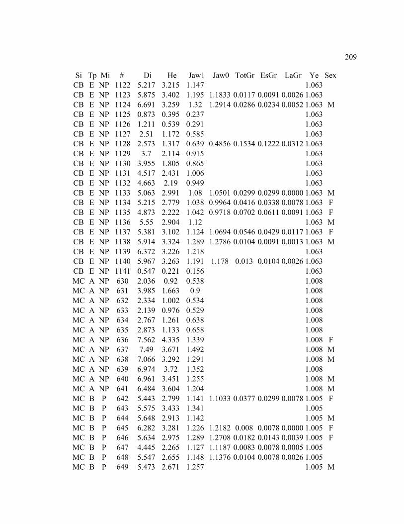
209
Si Tp Mi # Di He Jaw1 Jaw0 TotGr EsGr LaGr Ye Sex
CB E NP 1122 5.217 3.215 1.147 1.063
CB E NP 1123 5.875 3.402 1.195 1.1833 0.0117 0.0091 0.0026 1.063
CB E NP 1124 6.691 3.259 1.32 1.2914 0.0286 0.0234 0.0052 1.063 M
CB E NP 1125 0.873 0.395 0.237 1.063
CB E NP 1126 1.211 0.539 0.291 1.063
CB E NP 1127 2.51 1.172 0.585 1.063
CB E NP 1128 2.573 1.317 0.639 0.4856 0.1534 0.1222 0.0312 1.063
CB E NP 1129 3.7 2.114 0.915 1.063
CB E NP 1130 3.955 1.805 0.865 1.063
CB E NP 1131 4.517 2.431 1.006 1.063
CB E NP 1132 4.663 2.19 0.949 1.063
CB E NP 1133 5.063 2.991 1.08 1.0501 0.0299 0.0299 0.0000 1.063 M
CB E NP 1134 5.215 2.779 1.038 0.9964 0.0416 0.0338 0.0078 1.063 F
CB E NP 1135 4.873 2.222 1.042 0.9718 0.0702 0.0611 0.0091 1.063 F
CB E NP 1136 5.55 2.904 1.12 1.063 M
CB E NP 1137 5.381 3.102 1.124 1.0694 0.0546 0.0429 0.0117 1.063 F
CB E NP 1138 5.914 3.324 1.289 1.2786 0.0104 0.0091 0.0013 1.063 M
CB E NP 1139 6.372 3.226 1.218 1.063
CB E NP 1140 5.967 3.263 1.191 1.178 0.013 0.0104 0.0026 1.063
CB E NP 1141 0.547 0.221 0.156 1.063
MC A NP 630 2.036 0.92 0.538 1.008
MC A NP 631 3.985 1.663 0.9 1.008
MC A NP 632 2.334 1.002 0.534 1.008
MC A NP 633 2.139 0.976 0.529 1.008
MC A NP 634 2.767 1.261 0.638 1.008
MC A NP 635 2.873 1.133 0.658 1.008
MC A NP 636 7.562 4.335 1.339 1.008 F
MC A NP 637 7.49 3.671 1.492 1.008 M
MC A NP 638 7.066 3.292 1.291 1.008 M
MC A NP 639 6.974 3.72 1.352 1.008
MC A NP 640 6.961 3.451 1.255 1.008 M
MC A NP 641 6.484 3.604 1.204 1.008 M
MC B P 642 5.443 2.799 1.141 1.1033 0.0377 0.0299 0.0078 1.005 F
MC B P 643 5.575 3.433 1.341 1.005
MC B P 644 5.648 2.913 1.142 1.005 M
MC B P 645 6.282 3.281 1.226 1.2182 0.008 0.0078 0.0000 1.005 F
MC B P 646 5.634 2.975 1.289 1.2708 0.0182 0.0143 0.0039 1.005 F
MC B P 647 4.445 2.265 1.127 1.1187 0.0083 0.0078 0.0005 1.005
MC B P 648 5.547 2.655 1.148 1.1376 0.0104 0.0078 0.0026 1.005
MC B P 649 5.473 2.671 1.257 1.005 M
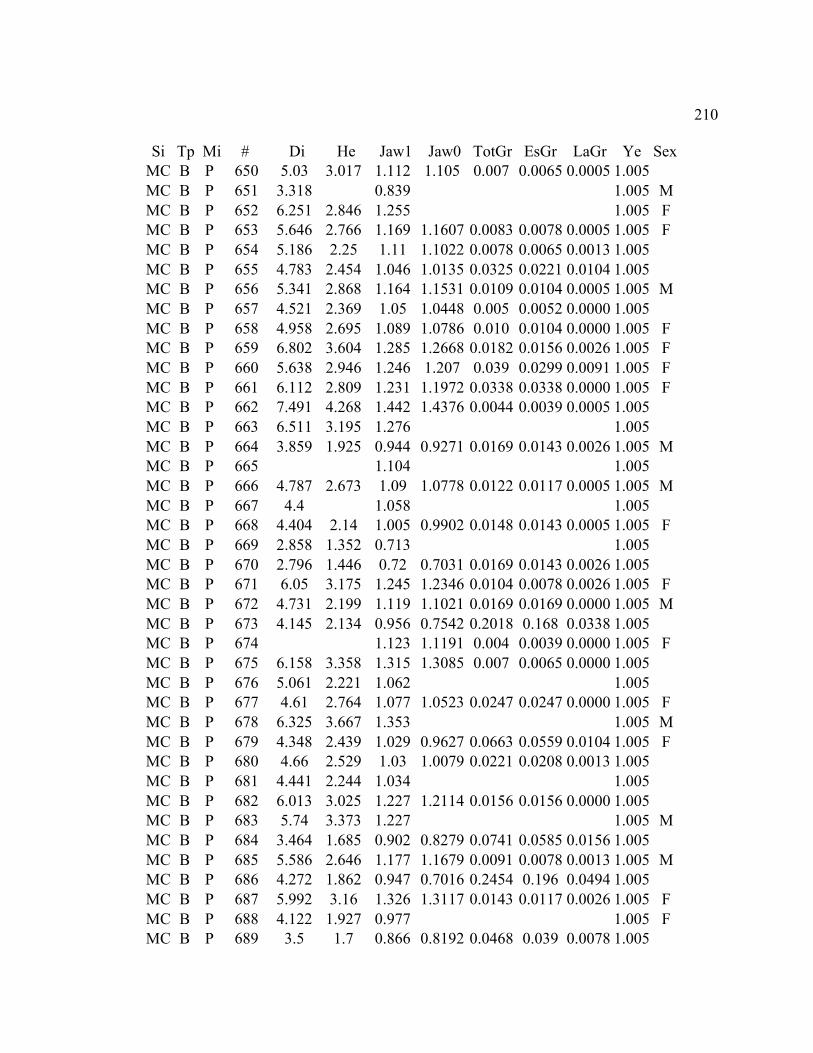
210
Si Tp Mi # Di He Jaw1 Jaw0 TotGr EsGr LaGr Ye Sex
MC B P 650 5.03 3.017 1.112 1.105 0.007 0.0065 0.0005 1.005
MC B P 651 3.318 0.839 1.005 M
MC B P 652 6.251 2.846 1.255 1.005 F
MC B P 653 5.646 2.766 1.169 1.1607 0.0083 0.0078 0.0005 1.005 F
MC B P 654 5.186 2.25 1.11 1.1022 0.0078 0.0065 0.0013 1.005
MC B P 655 4.783 2.454 1.046 1.0135 0.0325 0.0221 0.0104 1.005
MC B P 656 5.341 2.868 1.164 1.1531 0.0109 0.0104 0.0005 1.005 M
MC B P 657 4.521 2.369 1.05 1.0448 0.005 0.0052 0.0000 1.005
MC B P 658 4.958 2.695 1.089 1.0786 0.010 0.0104 0.0000 1.005 F
MC B P 659 6.802 3.604 1.285 1.2668 0.0182 0.0156 0.0026 1.005 F
MC B P 660 5.638 2.946 1.246 1.207 0.039 0.0299 0.0091 1.005 F
MC B P 661 6.112 2.809 1.231 1.1972 0.0338 0.0338 0.0000 1.005 F
MC B P 662 7.491 4.268 1.442 1.4376 0.0044 0.0039 0.0005 1.005
MC B P 663 6.511 3.195 1.276 1.005
MC B P 664 3.859 1.925 0.944 0.9271 0.0169 0.0143 0.0026 1.005 M
MC B P 665 1.104 1.005
MC B P 666 4.787 2.673 1.09 1.0778 0.0122 0.0117 0.0005 1.005 M
MC B P 667 4.4 1.058 1.005
MC B P 668 4.404 2.14 1.005 0.9902 0.0148 0.0143 0.0005 1.005 F
MC B P 669 2.858 1.352 0.713 1.005
MC B P 670 2.796 1.446 0.72 0.7031 0.0169 0.0143 0.0026 1.005
MC B P 671 6.05 3.175 1.245 1.2346 0.0104 0.0078 0.0026 1.005 F
MC B P 672 4.731 2.199 1.119 1.1021 0.0169 0.0169 0.0000 1.005 M
MC B P 673 4.145 2.134 0.956 0.7542 0.2018 0.168 0.0338 1.005
MC B P 674 1.123 1.1191 0.004 0.0039 0.0000 1.005 F
MC B P 675 6.158 3.358 1.315 1.3085 0.007 0.0065 0.0000 1.005
MC B P 676 5.061 2.221 1.062 1.005
MC B P 677 4.61 2.764 1.077 1.0523 0.0247 0.0247 0.0000 1.005 F
MC B P 678 6.325 3.667 1.353 1.005 M
MC B P 679 4.348 2.439 1.029 0.9627 0.0663 0.0559 0.0104 1.005 F
MC B P 680 4.66 2.529 1.03 1.0079 0.0221 0.0208 0.0013 1.005
MC B P 681 4.441 2.244 1.034 1.005
MC B P 682 6.013 3.025 1.227 1.2114 0.0156 0.0156 0.0000 1.005
MC B P 683 5.74 3.373 1.227 1.005 M
MC B P 684 3.464 1.685 0.902 0.8279 0.0741 0.0585 0.0156 1.005
MC B P 685 5.586 2.646 1.177 1.1679 0.0091 0.0078 0.0013 1.005 M
MC B P 686 4.272 1.862 0.947 0.7016 0.2454 0.196 0.0494 1.005
MC B P 687 5.992 3.16 1.326 1.3117 0.0143 0.0117 0.0026 1.005 F
MC B P 688 4.122 1.927 0.977 1.005 F
MC B P 689 3.5 1.7 0.866 0.8192 0.0468 0.039 0.0078 1.005

211
Si Tp Mi # Di He Jaw1 Jaw0 TotGr EsGr LaGr Ye Sex
MC B P 690 1.405 1.005
MC B P 691 0.864 0.7717 0.0923 0.0676 0.0247 1.005
MC B P 692 1.8 0.7 0.406 1.005
MC B P 693 5.491 2.721 1.19 1.1817 0.0083 0.0078 0.0005 1.005 F
MC B P 694 5.023 2.652 1.113 1.1091 0.004 0.0039 0.0000 1.005 F
MC B P 695 3.907 1.751 0.84 0.8296 0.010 0.0104 0.0000 1.005
MC B P 696 5.49 2.7 1.309 1.3064 0.003 0.0026 0.0000 1.005
MC B P 697 7.905 4.165 1.549 1.005 M
MC B P 698 6.804 3.027 1.299 1.005 M
MC B P 699 6.257 3.007 1.321 1.321 0.000 0.0000 0.0000 1.005 M
MC B P 700 6.638 3.197 1.378 1.005 M
MC B P 701 6.44 3.58 1.417 1.4022 0.0148 0.0143 0.0005 1.005 M
MC B P 702 6.443 3.655 1.16 1.1392 0.0208 0.0143 0.0065 1.005
MC B P 703 1.651 0.815 0.447 1.005
MC B NP 704 6.505 3.556 1.299 1.2881 0.0109 0.0104 0.0005 1.005 M
MC B NP 705 6.252 3.142 1.216 1.1861 0.0299 0.0247 0.0052 1.005
MC B NP 706 5.696 3.088 1.258 1.005 M
MC B NP 707 5.216 2.821 1.086 1.0418 0.0442 0.0416 0.0026 1.005
MC B NP 708 4.804 2.2 0.956 1.005
MC B NP 709 3.799 1.531 0.809 0.5591 0.2499 0.207 0.0429 1.005
MC B NP 710 6.036 2.874 1.257 1.005 F
MC B NP 711 6.411 3.054 1.348 1.3376 0.0104 0.0078 0.0026 1.005 F
MC B NP 712 5.151 2.315 1.033 1.005
MC B NP 713 6.301 3.129 1.158 1.005 M
MC B NP 714 5.958 3.1 1.156 1.0676 0.0884 0.0767 0.0117 1.005 M
MC B NP 715 6.321 2.951 1.296 1.005 M
MC B NP 716 6.009 2.909 1.178 1.005 M
MC B NP 717 6.028 3.242 1.248 1.005 M
MC B NP 718 5.927 3.061 1.291 1.005 F
MC B NP 719 5.117 2.25 1.017 1.005
MC B NP 720 2.966 1.209 0.647 0.2854 0.3616 0.294 0.0676 1.005
MC B NP 721 2.31 0.994 0.595 0.2236 0.3714 0.309 0.0624 1.005
MC B NP 722 6.015 3.192 1.178 1.1598 0.0182 0.013 0.0052 1.005 F
MC B NP 723 6.708 3.301 1.205 1.005 F
MC B NP 724 7.292 3.452 1.405 1.3972 0.0078 0.0065 0.0013 1.005 M
MC B NP 725 6.461 2.525 1.285 1.005 M
MC B NP 726 6.946 3.808 1.271 1.2606 0.010 0.0104 0.0000 1.005 M
MC B NP 727 7.211 3.411 1.397 1.005 M
MC B NP 728 6.215 3.434 1.246 1.2122 0.0338 0.0338 0.0000 1.005
MC B NP 729 6.589 3.086 1.287 1.005 F
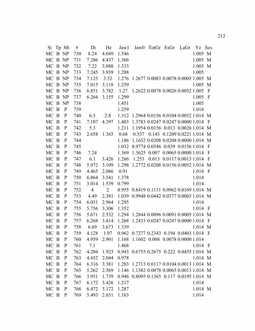
212
Si Tp Mi # Di He Jaw1 Jaw0 TotGr EsGr LaGr Ye Sex
MC B NP 730 8.24 4.049 1.546 1.005 M
MC B NP 731 7.286 4.437 1.366 1.005 M
MC B NP 732 7.22 3.888 1.333 1.005 M
MC B NP 733 7.245 3.939 1.288 1.005
MC B NP 734 7.125 3.52 1.276 1.2677 0.0083 0.0078 0.0005 1.005 M
MC B NP 735 7.015 3.118 1.259 1.005 M
MC B NP 736 6.851 3.782 1.27 1.2622 0.0078 0.0026 0.0052 1.005 F
MC B NP 737 6.264 3.155 1.299 1.005 F
MC B NP 738 1.451 1.005
MC B P 739 1.259 1.014
MC B P 740 6.5 2.8 1.312 1.2964 0.0156 0.0104 0.0052 1.014 M
MC B P 741 7.107 4.397 1.403 1.3783 0.0247 0.0247 0.0000 1.014 F
MC B P 742 5.3 1.211 1.1954 0.0156 0.013 0.0026 1.014 M
MC B P 743 2.658 1.365 0.68 0.537 0.143 0.1209 0.0221 1.014 M
MC B P 744 1.186 1.1652 0.0208 0.0208 0.0000 1.014 M
MC B P 745 1.032 0.9774 0.0546 0.039 0.0156 1.014 F
MC B P 746 7.24 1.369 1.3625 0.007 0.0065 0.0000 1.014 F
MC B P 747 6.1 3.426 1.266 1.253 0.013 0.0117 0.0013 1.014 F
MC B P 748 5.972 3.109 1.298 1.2772 0.0208 0.0156 0.0052 1.014 M
MC B P 749 4.465 2.086 0.91 1.014 F
MC B P 750 6.864 3.541 1.378 1.014
MC B P 751 3.014 1.539 0.799 1.014
MC B P 752 4 2 0.955 0.8419 0.1131 0.0962 0.0169 1.014 M
MC B P 753 4.49 2.381 1.039 0.9948 0.0442 0.0377 0.0065 1.014 M
MC B P 754 6.031 2.964 1.295 1.014
MC B P 755 5.756 3.306 1.352 1.014 F
MC B P 756 5.671 2.532 1.294 1.2844 0.0096 0.0091 0.0005 1.014 M
MC B P 757 6.268 3.414 1.268 1.2433 0.0247 0.0247 0.0000 1.014 F
MC B P 758 6.69 3.673 1.339 1.014 M
MC B P 759 4.128 1.97 0.962 0.7277 0.2343 0.194 0.0403 1.014 F
MC B P 760 4.959 2.901 1.168 1.1602 0.008 0.0078 0.0000 1.014
MC B P 761 7.1 1.468 1.014 F
MC B P 762 4.204 1.923 0.943 0.6755 0.2675 0.222 0.0455 1.014 M
MC B P 763 4.452 2.044 0.978 1.014 M
MC B P 764 6.316 3.381 1.283 1.2713 0.0117 0.0104 0.0013 1.014 M
MC B P 765 5.262 2.569 1.146 1.1382 0.0078 0.0065 0.0013 1.014 M
MC B P 766 3.951 1.739 0.946 0.8095 0.1365 0.117 0.0195 1.014 M
MC B P 767 6.172 3.426 1.217 1.014
MC B P 768 6.472 3.172 1.287 1.014 M
MC B P 769 5.493 2.651 1.163 1.014
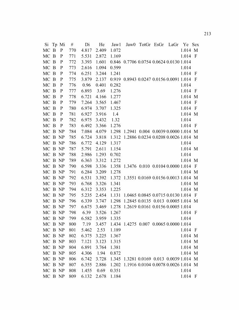
213
Si Tp Mi # Di He Jaw1 Jaw0 TotGr EsGr LaGr Ye Sex
MC B P 770 4.817 2.409 1.072 1.014 M
MC B P 771 5.531 2.872 1.169 1.014 F
MC B P 772 3.393 1.601 0.846 0.7706 0.0754 0.0624 0.0130 1.014
MC B P 773 2.616 1.094 0.599 1.014
MC B P 774 6.251 3.244 1.241 1.014 F
MC B P 775 3.879 2.137 0.919 0.8943 0.0247 0.0156 0.0091 1.014 F
MC B P 776 0.96 0.401 0.282 1.014
MC B P 777 6.893 3.69 1.276 1.014 F
MC B P 778 6.721 4.166 1.277 1.014 M
MC B P 779 7.264 3.565 1.467 1.014 F
MC B P 780 6.974 3.707 1.325 1.014 F
MC B P 781 6.927 3.916 1.4 1.014 M
MC B P 782 6.975 3.432 1.32 1.014
MC B P 783 6.492 3.366 1.276 1.014 F
MC B NP 784 7.084 4.079 1.298 1.2941 0.004 0.0039 0.0000 1.014 M
MC B NP 785 6.724 3.818 1.312 1.2886 0.0234 0.0208 0.0026 1.014 M
MC B NP 786 6.772 4.129 1.317 1.014
MC B NP 787 5.791 2.611 1.154 1.014 M
MC B NP 788 2.986 1.293 0.702 1.014
MC B NP 789 6.363 3.312 1.272 1.014 M
MC B NP 790 6.598 3.336 1.358 1.3476 0.010 0.0104 0.0000 1.014 F
MC B NP 791 6.284 3.209 1.278 1.014 M
MC B NP 792 6.531 3.392 1.372 1.3551 0.0169 0.0156 0.0013 1.014 M
MC B NP 793 6.768 3.326 1.341 1.014 M
MC B NP 794 6.312 3.353 1.225 1.014 M
MC B NP 795 5.235 2.454 1.131 1.0465 0.0845 0.0715 0.0130 1.014 F
MC B NP 796 6.339 3.747 1.298 1.2845 0.0135 0.013 0.0005 1.014 M
MC B NP 797 6.675 3.469 1.278 1.2619 0.0161 0.0156 0.0005 1.014
MC B NP 798 6.39 3.526 1.267 1.014 F
MC B NP 799 6.582 3.959 1.335 1.014
MC B NP 800 7.19 3.457 1.434 1.4275 0.007 0.0065 0.0000 1.014
MC B NP 801 5.462 2.53 1.189 1.014 F
MC B NP 802 6.375 3.225 1.367 1.014 M
MC B NP 803 7.121 3.123 1.315 1.014 M
MC B NP 804 6.891 3.764 1.381 1.014 M
MC B NP 805 4.306 1.94 0.872 1.014 M
MC B NP 806 6.742 3.728 1.345 1.3281 0.0169 0.013 0.0039 1.014 M
MC B NP 807 6.355 2.886 1.202 1.1916 0.0104 0.0078 0.0026 1.014 M
MC B NP 808 1.455 0.69 0.351 1.014
MC B NP 809 6.132 2.678 1.184 1.014 F
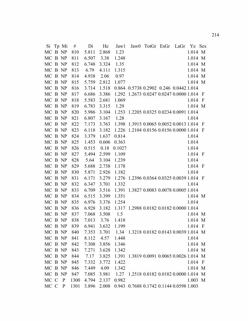
214
Si Tp Mi # Di He Jaw1 Jaw0 TotGr EsGr LaGr Ye Sex
MC B NP 810 5.811 2.868 1.23 1.014 M
MC B NP 811 6.507 3.38 1.248 1.014 M
MC B NP 812 6.748 3.324 1.35 1.014 M
MC B NP 813 6.79 4.111 1.315 1.014 M
MC B NP 814 4.938 2.06 0.97 1.014 M
MC B NP 815 5.759 2.812 1.077 1.014 M
MC B NP 816 3.714 1.518 0.864 0.5738 0.2902 0.246 0.0442 1.014
MC B NP 817 6.686 3.386 1.292 1.2673 0.0247 0.0247 0.0000 1.014 F
MC B NP 818 5.583 2.681 1.069 1.014 F
MC B NP 819 6.783 3.315 1.29 1.014 M
MC B NP 820 5.986 3.104 1.253 1.2205 0.0325 0.0234 0.0091 1.014
MC B NP 821 6.807 3.167 1.28 1.014
MC B NP 822 7.173 3.763 1.398 1.3915 0.0065 0.0052 0.0013 1.014 F
MC B NP 823 6.118 3.182 1.226 1.2104 0.0156 0.0156 0.0000 1.014 F
MC B NP 824 3.379 1.637 0.814 1.014
MC B NP 825 1.453 0.606 0.363 1.014
MC B NP 826 0.515 0.18 0.1027 1.014
MC B NP 827 5.494 2.599 1.109 1.014 F
MC B NP 828 5.64 3.104 1.239 1.014
MC B NP 829 5.688 2.738 1.178 1.014 F
MC B NP 830 5.871 2.926 1.182 1.014
MC B NP 831 6.171 3.279 1.276 1.2396 0.0364 0.0325 0.0039 1.014 F
MC B NP 832 6.347 3.701 1.332 1.014
MC B NP 833 6.709 3.516 1.391 1.3827 0.0083 0.0078 0.0005 1.014
MC B NP 834 6.515 3.399 1.351 1.014 M
MC B NP 835 6.976 3.376 1.254 1.014
MC B NP 836 6.928 3.182 1.317 1.2988 0.0182 0.0182 0.0000 1.014
MC B NP 837 7.068 3.508 1.5 1.014 M
MC B NP 838 7.013 3.76 1.418 1.014 M
MC B NP 839 6.941 3.632 1.199 1.014 F
MC B NP 840 7.353 3.701 1.34 1.3218 0.0182 0.0143 0.0039 1.014 M
MC B NP 841 8.112 4.57 1.448 1.014
MC B NP 842 7.308 3.856 1.346 1.014 M
MC B NP 843 7.271 3.628 1.342 1.014 M
MC B NP 844 7.17 3.825 1.391 1.3819 0.0091 0.0065 0.0026 1.014 M
MC B NP 845 7.332 3.772 1.422 1.014 F
MC B NP 846 7.449 4.09 1.342 1.014 M
MC B NP 847 7.085 3.981 1.27 1.2518 0.0182 0.0182 0.0000 1.014 M
MC C P 1300 4.794 2.137 0.982 1.003 M
MC C P 1301 3.896 2.008 0.943 0.7688 0.1742 0.1144 0.0598 1.003
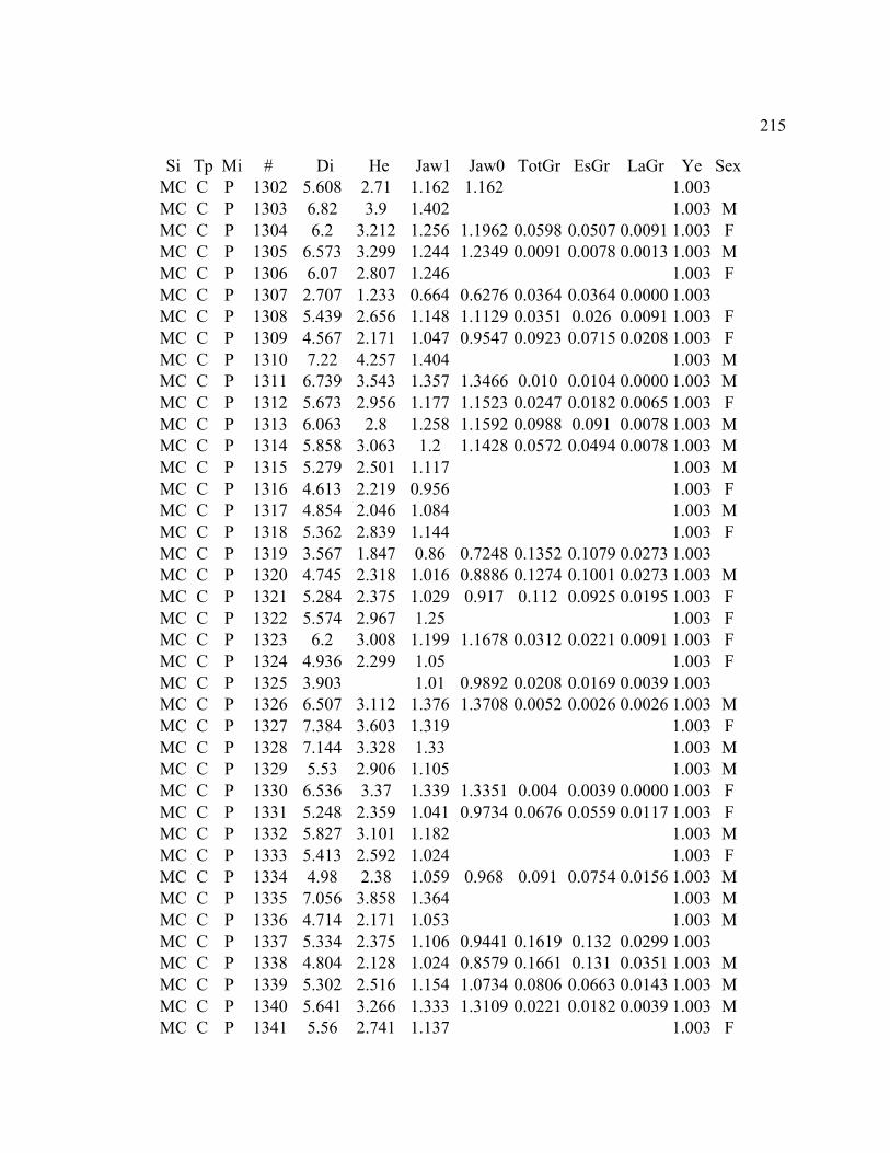
215
Si Tp Mi # Di He Jaw1 Jaw0 TotGr EsGr LaGr Ye Sex
MC C P 1302 5.608 2.71 1.162 1.162 1.003
MC C P 1303 6.82 3.9 1.402 1.003 M
MC C P 1304 6.2 3.212 1.256 1.1962 0.0598 0.0507 0.0091 1.003 F
MC C P 1305 6.573 3.299 1.244 1.2349 0.0091 0.0078 0.0013 1.003 M
MC C P 1306 6.07 2.807 1.246 1.003 F
MC C P 1307 2.707 1.233 0.664 0.6276 0.0364 0.0364 0.0000 1.003
MC C P 1308 5.439 2.656 1.148 1.1129 0.0351 0.026 0.0091 1.003 F
MC C P 1309 4.567 2.171 1.047 0.9547 0.0923 0.0715 0.0208 1.003 F
MC C P 1310 7.22 4.257 1.404 1.003 M
MC C P 1311 6.739 3.543 1.357 1.3466 0.010 0.0104 0.0000 1.003 M
MC C P 1312 5.673 2.956 1.177 1.1523 0.0247 0.0182 0.0065 1.003 F
MC C P 1313 6.063 2.8 1.258 1.1592 0.0988 0.091 0.0078 1.003 M
MC C P 1314 5.858 3.063 1.2 1.1428 0.0572 0.0494 0.0078 1.003 M
MC C P 1315 5.279 2.501 1.117 1.003 M
MC C P 1316 4.613 2.219 0.956 1.003 F
MC C P 1317 4.854 2.046 1.084 1.003 M
MC C P 1318 5.362 2.839 1.144 1.003 F
MC C P 1319 3.567 1.847 0.86 0.7248 0.1352 0.1079 0.0273 1.003
MC C P 1320 4.745 2.318 1.016 0.8886 0.1274 0.1001 0.0273 1.003 M
MC C P 1321 5.284 2.375 1.029 0.917 0.112 0.0925 0.0195 1.003 F
MC C P 1322 5.574 2.967 1.25 1.003 F
MC C P 1323 6.2 3.008 1.199 1.1678 0.0312 0.0221 0.0091 1.003 F
MC C P 1324 4.936 2.299 1.05 1.003 F
MC C P 1325 3.903 1.01 0.9892 0.0208 0.0169 0.0039 1.003
MC C P 1326 6.507 3.112 1.376 1.3708 0.0052 0.0026 0.0026 1.003 M
MC C P 1327 7.384 3.603 1.319 1.003 F
MC C P 1328 7.144 3.328 1.33 1.003 M
MC C P 1329 5.53 2.906 1.105 1.003 M
MC C P 1330 6.536 3.37 1.339 1.3351 0.004 0.0039 0.0000 1.003 F
MC C P 1331 5.248 2.359 1.041 0.9734 0.0676 0.0559 0.0117 1.003 F
MC C P 1332 5.827 3.101 1.182 1.003 M
MC C P 1333 5.413 2.592 1.024 1.003 F
MC C P 1334 4.98 2.38 1.059 0.968 0.091 0.0754 0.0156 1.003 M
MC C P 1335 7.056 3.858 1.364 1.003 M
MC C P 1336 4.714 2.171 1.053 1.003 M
MC C P 1337 5.334 2.375 1.106 0.9441 0.1619 0.132 0.0299 1.003
MC C P 1338 4.804 2.128 1.024 0.8579 0.1661 0.131 0.0351 1.003 M
MC C P 1339 5.302 2.516 1.154 1.0734 0.0806 0.0663 0.0143 1.003 M
MC C P 1340 5.641 3.266 1.333 1.3109 0.0221 0.0182 0.0039 1.003 M
MC C P 1341 5.56 2.741 1.137 1.003 F
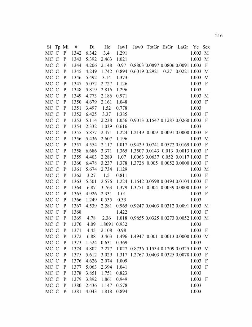
216
Si Tp Mi # Di He Jaw1 Jaw0 TotGr EsGr LaGr Ye Sex
MC C P 1342 6.342 3.4 1.291 1.003 M
MC C P 1343 5.392 2.463 1.021 1.003 M
MC C P 1344 4.206 2.148 0.97 0.8803 0.0897 0.0806 0.0091 1.003 F
MC C P 1345 4.249 1.742 0.894 0.6019 0.2921 0.27 0.0221 1.003 M
MC C P 1346 5.492 3.14 1.373 1.003 M
MC C P 1347 5.072 2.727 1.126 1.003 F
MC C P 1348 5.819 2.816 1.296 1.003
MC C P 1349 4.773 2.186 0.971 1.003 M
MC C P 1350 4.679 2.161 1.048 1.003 F
MC C P 1351 3.497 1.52 0.778 1.003
MC C P 1352 6.425 3.37 1.385 1.003 F
MC C P 1353 5.114 2.238 1.056 0.9013 0.1547 0.1287 0.0260 1.003 F
MC C P 1354 2.332 1.039 0.616 1.003
MC C P 1355 5.877 2.471 1.224 1.2149 0.009 0.0091 0.0000 1.003 F
MC C P 1356 5.436 2.607 1.196 1.003 M
MC C P 1357 4.554 2.117 1.017 0.9429 0.0741 0.0572 0.0169 1.003 F
MC C P 1358 6.686 3.371 1.365 1.3507 0.0143 0.013 0.0013 1.003 F
MC C P 1359 4.403 2.289 1.07 1.0063 0.0637 0.052 0.0117 1.003 F
MC C P 1360 6.478 3.237 1.378 1.3728 0.005 0.0052 0.0000 1.003 F
MC C P 1361 5.674 2.734 1.129 1.003 M
MC C P 1362 3.27 1.5 0.811 1.003 F
MC C P 1363 5.501 2.576 1.224 1.1642 0.0598 0.0494 0.0104 1.003 F
MC C P 1364 6.87 3.763 1.379 1.3751 0.004 0.0039 0.0000 1.003 F
MC C P 1365 4.926 2.331 1.01 1.003 F
MC C P 1366 1.249 0.535 0.33 1.003
MC C P 1367 4.539 2.281 0.965 0.9247 0.0403 0.0312 0.0091 1.003 M
MC C P 1368 1.422 1.003 F
MC C P 1369 4.78 2.36 1.018 0.9855 0.0325 0.0273 0.0052 1.003 M
MC C P 1370 4.09 1.8091 0.932 1.003
MC C P 1371 4.45 2.108 0.98 1.003 F
MC C P 1372 6.88 3.463 1.496 1.4947 0.001 0.0013 0.0000 1.003 M
MC C P 1373 1.524 0.631 0.369 1.003
MC C P 1374 4.802 2.277 1.027 0.8736 0.1534 0.1209 0.0325 1.003 M
MC C P 1375 5.612 3.029 1.317 1.2767 0.0403 0.0325 0.0078 1.003 F
MC C P 1376 4.626 2.074 1.009 1.003 F
MC C P 1377 5.063 2.394 1.041 1.003 F
MC C P 1378 3.851 1.751 0.823 1.003
MC C P 1379 3.892 1.861 0.949 1.003 F
MC C P 1380 2.436 1.147 0.578 1.003
MC C P 1381 4.043 1.818 0.894 1.003

217
Si Tp Mi # Di He Jaw1 Jaw0 TotGr EsGr LaGr Ye Sex
MC C P 1382 5.965 2.795 1.194 1.0796 0.1144 0.0897 0.0247 1.003
MC C P 1383 5.709 2.892 1.216 1.1939 0.0221 0.0182 0.0039 1.003 F
MC C P 1384 5.648 2.565 1.094 1.003 F
MC C P 1385 5.106 2.206 1.122 1.0401 0.0819 0.0637 0.0182 1.003 F
MC C P 1386 3.533 1.592 0.84 1.003
MC C P 1387 5.258 2.509 1.116 1.0562 0.0598 0.052 0.0078 1.003 M
MC C P 1388 4.666 2.142 0.962 1.003
MC C P 1389 3.797 1.643 0.833 1.003
MC C P 1390 6.663 3.43 1.375 1.3659 0.009 0.0091 0.0000 1.003 M
MC C P 1391 7.343 4.03 1.369 1.003 M
MC C P 1392 7.367 3.932 1.496 1.003 M
MC C P 1393 7.939 3.879 1.448 1.4402 0.008 0.0078 0.0000 1.003 F
MC C P 1394 7.426 3.817 1.355 1.3549 0.000 0.0001 0.0000 1.003 F
MC C P 1395 7.322 4.37 1.524 1.003 M
MC C P 1396 7.515 3.725 1.576 1.563 0.013 0.013 0.0000 1.003 F
MC C P 1397 7.437 3.191 1.415 1.4072 0.0078 0.0052 0.0026 1.003 M
MC C P 1398 7.446 3.711 1.474 1.4701 0.004 0.0039 0.0000 1.003 M
MC C P 1399 7.711 3.911 1.532 1.003 F
MC C P 1400 3.333 1.412 0.745 1.003
MC C P 1401 3.576 1.577 0.761 1.003
MC C P 1402 4.892 1.94 1.019 1.003
MC C NP 1403 7.378 3.217 1.437 1.003
MC C NP 1404 2.02 0.94 0.466 1.003
MC C NP 1405 1.838 0.864 0.424 1.003
MC C NP 1406 1.212 0.548 0.315 1.003
MC C NP 1407 1.266 0.575 0.314 1.003
MC C NP 1408 1.33 0.643 0.338 1.003
MC C NP 1409 1.236 0.531 0.328 1.003
MC C NP 1410 1.452 0.664 0.372 1.003
MC C NP 1411 7.141 3.137 1.279 1.003 M
MC C NP 1412 6.95 3.419 1.318 1.003 F
MC C NP 1413 6.89 3.523 1.362 1.003 M
MC C NP 1414 6.714 3.02 1.346 1.3421 0.004 0.0039 0.0000 1.003 M
MC C NP 1415 4.996 2.482 1.05 1.003 F
MC C NP 1416 5.293 2.322 1.043 1.003 F
MC C NP 1417 5.237 2.559 1.107 1.0654 0.0416 0.0416 0.0000 1.003 M
MC C NP 1418 6.962 3.483 1.412 1.003 M
MC C NP 1419 5.265 2.746 1.222 1.2168 0.0052 0.0039 0.0013 1.003 M
MC C NP 1420 5.94 2.981 1.206 1.003 M
MC C NP 1421 6.629 3.91 1.433 1.003 M
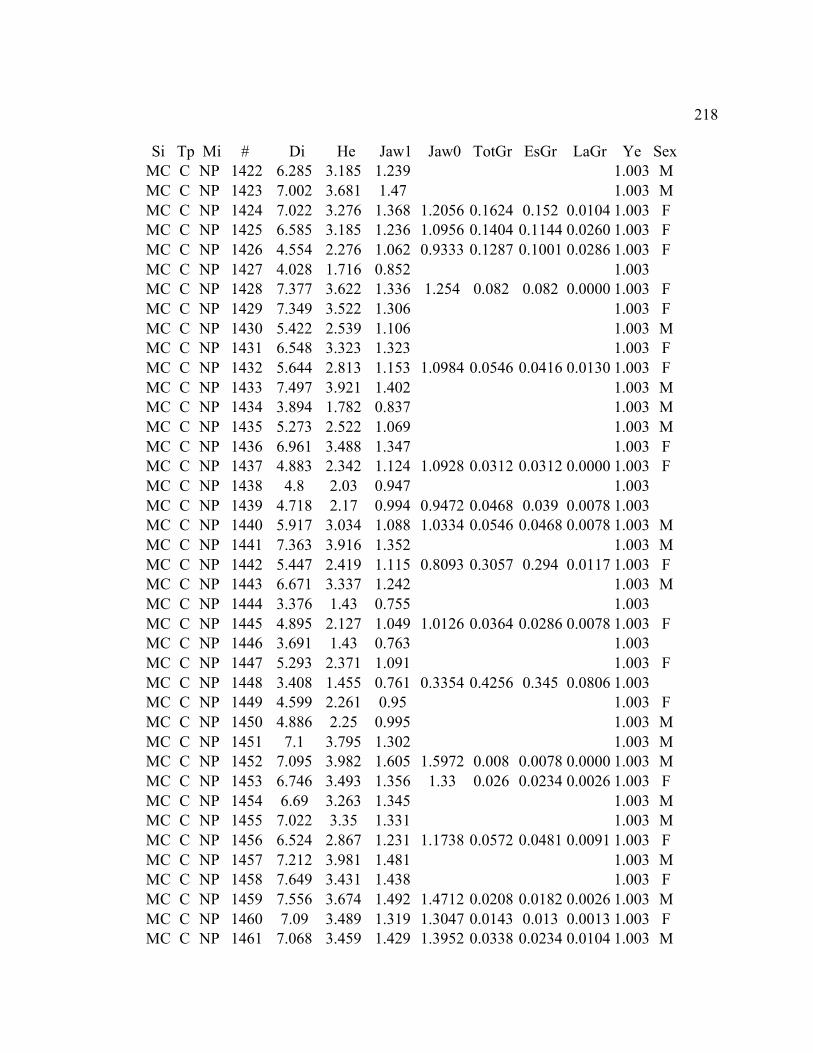
218
Si Tp Mi # Di He Jaw1 Jaw0 TotGr EsGr LaGr Ye Sex
MC C NP 1422 6.285 3.185 1.239 1.003 M
MC C NP 1423 7.002 3.681 1.47 1.003 M
MC C NP 1424 7.022 3.276 1.368 1.2056 0.1624 0.152 0.0104 1.003 F
MC C NP 1425 6.585 3.185 1.236 1.0956 0.1404 0.1144 0.0260 1.003 F
MC C NP 1426 4.554 2.276 1.062 0.9333 0.1287 0.1001 0.0286 1.003 F
MC C NP 1427 4.028 1.716 0.852 1.003
MC C NP 1428 7.377 3.622 1.336 1.254 0.082 0.082 0.0000 1.003 F
MC C NP 1429 7.349 3.522 1.306 1.003 F
MC C NP 1430 5.422 2.539 1.106 1.003 M
MC C NP 1431 6.548 3.323 1.323 1.003 F
MC C NP 1432 5.644 2.813 1.153 1.0984 0.0546 0.0416 0.0130 1.003 F
MC C NP 1433 7.497 3.921 1.402 1.003 M
MC C NP 1434 3.894 1.782 0.837 1.003 M
MC C NP 1435 5.273 2.522 1.069 1.003 M
MC C NP 1436 6.961 3.488 1.347 1.003 F
MC C NP 1437 4.883 2.342 1.124 1.0928 0.0312 0.0312 0.0000 1.003 F
MC C NP 1438 4.8 2.03 0.947 1.003
MC C NP 1439 4.718 2.17 0.994 0.9472 0.0468 0.039 0.0078 1.003
MC C NP 1440 5.917 3.034 1.088 1.0334 0.0546 0.0468 0.0078 1.003 M
MC C NP 1441 7.363 3.916 1.352 1.003 M
MC C NP 1442 5.447 2.419 1.115 0.8093 0.3057 0.294 0.0117 1.003 F
MC C NP 1443 6.671 3.337 1.242 1.003 M
MC C NP 1444 3.376 1.43 0.755 1.003
MC C NP 1445 4.895 2.127 1.049 1.0126 0.0364 0.0286 0.0078 1.003 F
MC C NP 1446 3.691 1.43 0.763 1.003
MC C NP 1447 5.293 2.371 1.091 1.003 F
MC C NP 1448 3.408 1.455 0.761 0.3354 0.4256 0.345 0.0806 1.003
MC C NP 1449 4.599 2.261 0.95 1.003 F
MC C NP 1450 4.886 2.25 0.995 1.003 M
MC C NP 1451 7.1 3.795 1.302 1.003 M
MC C NP 1452 7.095 3.982 1.605 1.5972 0.008 0.0078 0.0000 1.003 M
MC C NP 1453 6.746 3.493 1.356 1.33 0.026 0.0234 0.0026 1.003 F
MC C NP 1454 6.69 3.263 1.345 1.003 M
MC C NP 1455 7.022 3.35 1.331 1.003 M
MC C NP 1456 6.524 2.867 1.231 1.1738 0.0572 0.0481 0.0091 1.003 F
MC C NP 1457 7.212 3.981 1.481 1.003 M
MC C NP 1458 7.649 3.431 1.438 1.003 F
MC C NP 1459 7.556 3.674 1.492 1.4712 0.0208 0.0182 0.0026 1.003 M
MC C NP 1460 7.09 3.489 1.319 1.3047 0.0143 0.013 0.0013 1.003 F
MC C NP 1461 7.068 3.459 1.429 1.3952 0.0338 0.0234 0.0104 1.003 M
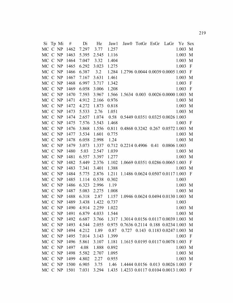
219
Si Tp Mi # Di He Jaw1 Jaw0 TotGr EsGr LaGr Ye Sex
MC C NP 1462 7.297 3.77 1.257 1.003 M
MC C NP 1463 5.395 2.545 1.116 1.003 M
MC C NP 1464 7.047 3.32 1.404 1.003 M
MC C NP 1465 6.292 3.023 1.275 1.003 F
MC C NP 1466 6.387 3.2 1.284 1.2796 0.0044 0.0039 0.0005 1.003 F
MC C NP 1467 7.167 3.631 1.461 1.003 M
MC C NP 1468 6.997 3.717 1.342 1.003 F
MC C NP 1469 6.058 3.006 1.208 1.003 F
MC C NP 1470 7.593 3.967 1.566 1.5634 0.003 0.0026 0.0000 1.003 M
MC C NP 1471 4.912 2.166 0.976 1.003 M
MC C NP 1472 4.272 1.873 0.818 1.003 M
MC C NP 1473 5.533 2.76 1.051 1.003 M
MC C NP 1474 2.657 1.074 0.58 0.5449 0.0351 0.0325 0.0026 1.003
MC C NP 1475 7.576 3.543 1.468 1.003 F
MC C NP 1476 3.868 1.556 0.811 0.4868 0.3242 0.267 0.0572 1.003 M
MC C NP 1477 3.534 1.601 0.775 1.003 M
MC C NP 1478 6.058 2.998 1.24 1.003 M
MC C NP 1479 3.073 1.337 0.712 0.2214 0.4906 0.41 0.0806 1.003
MC C NP 1480 5.03 2.547 1.039 1.003 M
MC C NP 1481 6.557 3.397 1.277 1.003 M
MC C NP 1482 5.449 2.376 1.102 1.0669 0.0351 0.0286 0.0065 1.003 F
MC C NP 1483 7.341 3.401 1.388 1.003 M
MC C NP 1484 5.775 2.876 1.211 1.1486 0.0624 0.0507 0.0117 1.003 F
MC C NP 1485 1.114 0.538 0.302 1.003
MC C NP 1486 6.323 2.996 1.19 1.003 M
MC C NP 1487 5.083 2.275 1.008 1.003 M
MC C NP 1488 6.318 2.87 1.157 1.0946 0.0624 0.0494 0.0130 1.003 M
MC C NP 1489 3.438 1.422 0.737 1.003
MC C NP 1490 4.914 2.259 1.022 1.003 M
MC C NP 1491 6.879 4.033 1.544 1.003 M
MC C NP 1492 6.687 3.766 1.317 1.3014 0.0156 0.0117 0.0039 1.003 M
MC C NP 1493 4.544 2.055 0.975 0.7636 0.2114 0.188 0.0234 1.003 M
MC C NP 1494 4.212 1.89 0.87 0.727 0.143 0.1183 0.0247 1.003 M
MC C NP 1495 7.014 3.143 1.399 1.003 F
MC C NP 1496 5.861 3.107 1.181 1.1615 0.0195 0.0117 0.0078 1.003 F
MC C NP 1497 4.08 1.888 0.892 1.003 M
MC C NP 1498 5.582 2.707 1.095 1.003 M
MC C NP 1499 4.802 2.27 0.955 1.003 M
MC C NP 1500 6.905 3.75 1.46 1.4444 0.0156 0.013 0.0026 1.003 F
MC C NP 1501 7.031 3.294 1.435 1.4233 0.0117 0.0104 0.0013 1.003 F
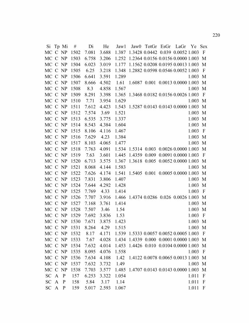
220
Si Tp Mi # Di He Jaw1 Jaw0 TotGr EsGr LaGr Ye Sex
MC C NP 1502 7.081 3.688 1.387 1.3428 0.0442 0.039 0.0052 1.003 F
MC C NP 1503 6.758 3.206 1.252 1.2364 0.0156 0.0156 0.0000 1.003 M
MC C NP 1504 6.023 3.019 1.177 1.1562 0.0208 0.0195 0.0013 1.003 M
MC C NP 1505 6.25 3.218 1.348 1.2882 0.0598 0.0546 0.0052 1.003 F
MC C NP 1506 6.641 3.591 1.289 1.003 M
MC C NP 1507 8.666 4.502 1.61 1.6087 0.001 0.0013 0.0000 1.003 M
MC C NP 1508 8.3 4.858 1.567 1.003 M
MC C NP 1509 8.291 3.398 1.365 1.3468 0.0182 0.0156 0.0026 1.003 F
MC C NP 1510 7.71 3.954 1.629 1.003 M
MC C NP 1511 7.612 4.423 1.543 1.5287 0.0143 0.0143 0.0000 1.003 M
MC C NP 1512 7.574 3.69 1.521 1.003 M
MC C NP 1513 6.535 3.775 1.337 1.003 M
MC C NP 1514 8.543 4.384 1.604 1.003 M
MC C NP 1515 8.106 4.116 1.467 1.003 F
MC C NP 1516 7.629 4.23 1.384 1.003 M
MC C NP 1517 8.103 4.065 1.477 1.003 M
MC C NP 1518 7.763 4.091 1.534 1.5314 0.003 0.0026 0.0000 1.003 M
MC C NP 1519 7.63 3.601 1.445 1.4359 0.009 0.0091 0.0000 1.003 F
MC C NP 1520 6.713 3.575 1.367 1.3618 0.005 0.0052 0.0000 1.003 M
MC C NP 1521 8.068 4.144 1.583 1.003 M
MC C NP 1522 7.626 4.174 1.541 1.5405 0.001 0.0005 0.0000 1.003 M
MC C NP 1523 7.831 3.806 1.407 1.003 M
MC C NP 1524 7.644 4.292 1.428 1.003 M
MC C NP 1525 7.769 4.33 1.414 1.003 F
MC C NP 1526 7.707 3.916 1.466 1.4374 0.0286 0.026 0.0026 1.003 M
MC C NP 1527 7.168 3.761 1.414 1.003 M
MC C NP 1528 7.507 3.46 1.54 1.003 M
MC C NP 1529 7.692 3.836 1.53 1.003 F
MC C NP 1530 7.671 3.875 1.423 1.003 M
MC C NP 1531 8.264 4.29 1.515 1.003 M
MC C NP 1532 8.17 4.171 1.539 1.5333 0.0057 0.0052 0.0005 1.003 F
MC C NP 1533 7.67 4.028 1.434 1.4339 0.000 0.0001 0.0000 1.003 M
MC C NP 1534 7.632 4.014 1.453 1.4426 0.010 0.0104 0.0000 1.003 M
MC C NP 1535 8.095 4.076 1.558 1.003 F
MC C NP 1536 7.634 4.108 1.42 1.4122 0.0078 0.0065 0.0013 1.003 M
MC C NP 1537 7.632 3.732 1.49 1.003 M
MC C NP 1538 7.703 3.577 1.485 1.4707 0.0143 0.0143 0.0000 1.003 M
SC A P 157 6.253 3.322 1.054 1.011 F
SC A P 158 5.84 3.17 1.14 1.011 F
SC A P 159 5.017 2.593 1.067 1.011 F
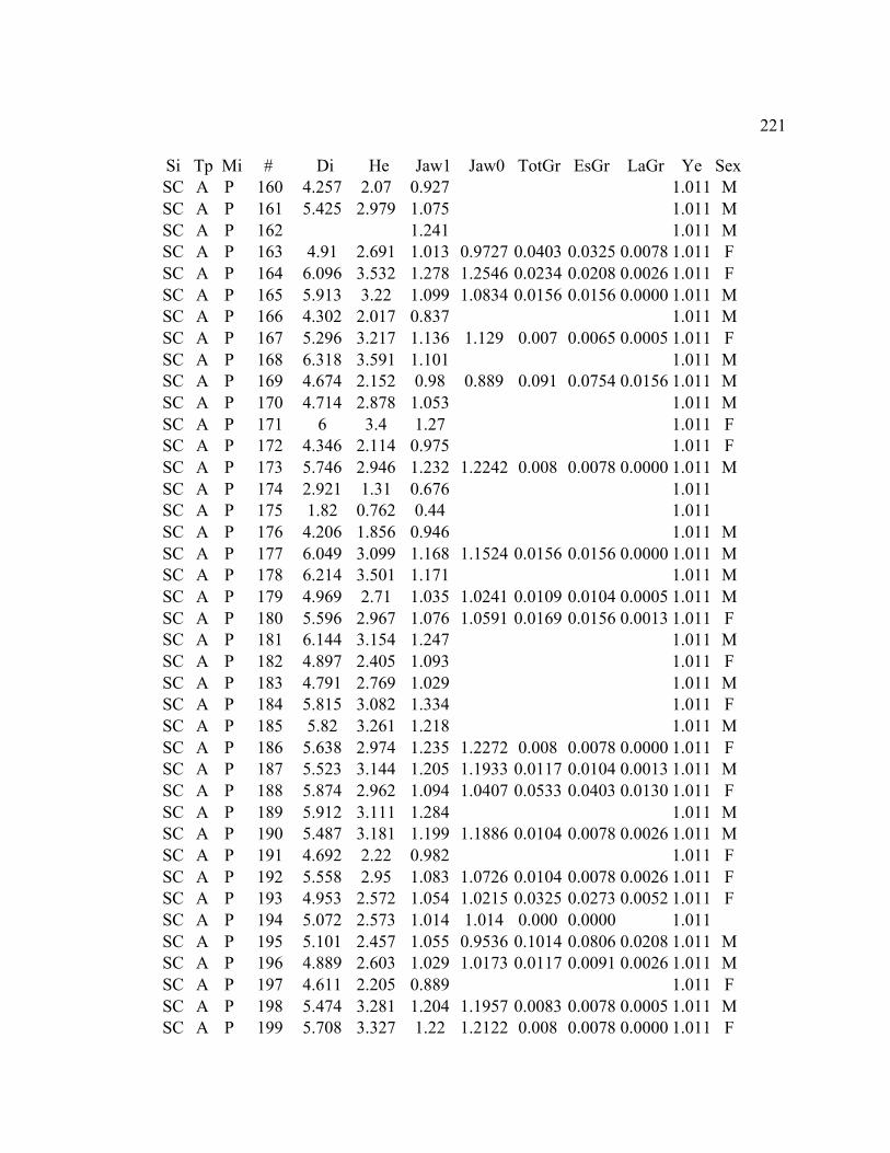
221
Si Tp Mi # Di He Jaw1 Jaw0 TotGr EsGr LaGr Ye Sex
SC A P 160 4.257 2.07 0.927 1.011 M
SC A P 161 5.425 2.979 1.075 1.011 M
SC A P 162 1.241 1.011 M
SC A P 163 4.91 2.691 1.013 0.9727 0.0403 0.0325 0.0078 1.011 F
SC A P 164 6.096 3.532 1.278 1.2546 0.0234 0.0208 0.0026 1.011 F
SC A P 165 5.913 3.22 1.099 1.0834 0.0156 0.0156 0.0000 1.011 M
SC A P 166 4.302 2.017 0.837 1.011 M
SC A P 167 5.296 3.217 1.136 1.129 0.007 0.0065 0.0005 1.011 F
SC A P 168 6.318 3.591 1.101 1.011 M
SC A P 169 4.674 2.152 0.98 0.889 0.091 0.0754 0.0156 1.011 M
SC A P 170 4.714 2.878 1.053 1.011 M
SC A P 171 6 3.4 1.27 1.011 F
SC A P 172 4.346 2.114 0.975 1.011 F
SC A P 173 5.746 2.946 1.232 1.2242 0.008 0.0078 0.0000 1.011 M
SC A P 174 2.921 1.31 0.676 1.011
SC A P 175 1.82 0.762 0.44 1.011
SC A P 176 4.206 1.856 0.946 1.011 M
SC A P 177 6.049 3.099 1.168 1.1524 0.0156 0.0156 0.0000 1.011 M
SC A P 178 6.214 3.501 1.171 1.011 M
SC A P 179 4.969 2.71 1.035 1.0241 0.0109 0.0104 0.0005 1.011 M
SC A P 180 5.596 2.967 1.076 1.0591 0.0169 0.0156 0.0013 1.011 F
SC A P 181 6.144 3.154 1.247 1.011 M
SC A P 182 4.897 2.405 1.093 1.011 F
SC A P 183 4.791 2.769 1.029 1.011 M
SC A P 184 5.815 3.082 1.334 1.011 F
SC A P 185 5.82 3.261 1.218 1.011 M
SC A P 186 5.638 2.974 1.235 1.2272 0.008 0.0078 0.0000 1.011 F
SC A P 187 5.523 3.144 1.205 1.1933 0.0117 0.0104 0.0013 1.011 M
SC A P 188 5.874 2.962 1.094 1.0407 0.0533 0.0403 0.0130 1.011 F
SC A P 189 5.912 3.111 1.284 1.011 M
SC A P 190 5.487 3.181 1.199 1.1886 0.0104 0.0078 0.0026 1.011 M
SC A P 191 4.692 2.22 0.982 1.011 F
SC A P 192 5.558 2.95 1.083 1.0726 0.0104 0.0078 0.0026 1.011 F
SC A P 193 4.953 2.572 1.054 1.0215 0.0325 0.0273 0.0052 1.011 F
SC A P 194 5.072 2.573 1.014 1.014 0.000 0.0000 1.011
SC A P 195 5.101 2.457 1.055 0.9536 0.1014 0.0806 0.0208 1.011 M
SC A P 196 4.889 2.603 1.029 1.0173 0.0117 0.0091 0.0026 1.011 M
SC A P 197 4.611 2.205 0.889 1.011 F
SC A P 198 5.474 3.281 1.204 1.1957 0.0083 0.0078 0.0005 1.011 M
SC A P 199 5.708 3.327 1.22 1.2122 0.008 0.0078 0.0000 1.011 F
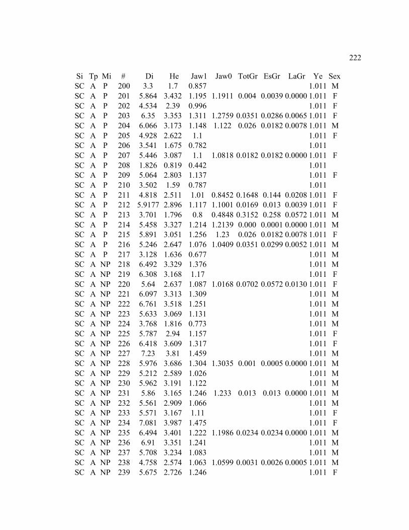
222
Si Tp Mi # Di He Jaw1 Jaw0 TotGr EsGr LaGr Ye Sex
SC A P 200 3.3 1.7 0.857 1.011 M
SC A P 201 5.864 3.432 1.195 1.1911 0.004 0.0039 0.0000 1.011 F
SC A P 202 4.534 2.39 0.996 1.011 F
SC A P 203 6.35 3.353 1.311 1.2759 0.0351 0.0286 0.0065 1.011 F
SC A P 204 6.066 3.173 1.148 1.122 0.026 0.0182 0.0078 1.011 M
SC A P 205 4.928 2.622 1.1 1.011 F
SC A P 206 3.541 1.675 0.782 1.011
SC A P 207 5.446 3.087 1.1 1.0818 0.0182 0.0182 0.0000 1.011 F
SC A P 208 1.826 0.819 0.442 1.011
SC A P 209 5.064 2.803 1.137 1.011 F
SC A P 210 3.502 1.59 0.787 1.011
SC A P 211 4.818 2.511 1.01 0.8452 0.1648 0.144 0.0208 1.011 F
SC A P 212 5.9177 2.896 1.117 1.1001 0.0169 0.013 0.0039 1.011 F
SC A P 213 3.701 1.796 0.8 0.4848 0.3152 0.258 0.0572 1.011 M
SC A P 214 5.458 3.327 1.214 1.2139 0.000 0.0001 0.0000 1.011 M
SC A P 215 5.891 3.051 1.256 1.23 0.026 0.0182 0.0078 1.011 F
SC A P 216 5.246 2.647 1.076 1.0409 0.0351 0.0299 0.0052 1.011 M
SC A P 217 3.128 1.636 0.677 1.011 M
SC A NP 218 6.492 3.329 1.376 1.011 M
SC A NP 219 6.308 3.168 1.17 1.011 F
SC A NP 220 5.64 2.637 1.087 1.0168 0.0702 0.0572 0.0130 1.011 F
SC A NP 221 6.097 3.313 1.309 1.011 M
SC A NP 222 6.761 3.518 1.251 1.011 M
SC A NP 223 5.633 3.069 1.131 1.011 M
SC A NP 224 3.768 1.816 0.773 1.011 M
SC A NP 225 5.787 2.94 1.157 1.011 F
SC A NP 226 6.418 3.609 1.317 1.011 F
SC A NP 227 7.23 3.81 1.459 1.011 M
SC A NP 228 5.976 3.686 1.304 1.3035 0.001 0.0005 0.0000 1.011 M
SC A NP 229 5.212 2.589 1.026 1.011 M
SC A NP 230 5.962 3.191 1.122 1.011 M
SC A NP 231 5.86 3.165 1.246 1.233 0.013 0.013 0.0000 1.011 M
SC A NP 232 5.561 2.909 1.066 1.011 M
SC A NP 233 5.571 3.167 1.11 1.011 F
SC A NP 234 7.081 3.987 1.475 1.011 F
SC A NP 235 6.494 3.401 1.222 1.1986 0.0234 0.0234 0.0000 1.011 M
SC A NP 236 6.91 3.351 1.241 1.011 M
SC A NP 237 5.708 3.234 1.083 1.011 M
SC A NP 238 4.758 2.574 1.063 1.0599 0.0031 0.0026 0.0005 1.011 M
SC A NP 239 5.675 2.726 1.246 1.011 F
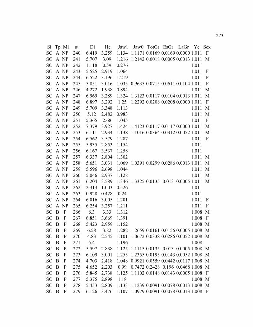
223
Si Tp Mi # Di He Jaw1 Jaw0 TotGr EsGr LaGr Ye Sex
SC A NP 240 6.419 3.259 1.134 1.1171 0.0169 0.0169 0.0000 1.011 F
SC A NP 241 5.707 3.09 1.216 1.2142 0.0018 0.0005 0.0013 1.011 M
SC A NP 242 1.118 0.59 0.276 1.011
SC A NP 243 5.525 2.919 1.064 1.011 F
SC A NP 244 6.522 3.196 1.219 1.011 F
SC A NP 245 5.851 3.016 1.035 0.9635 0.0715 0.0611 0.0104 1.011 F
SC A NP 246 4.272 1.938 0.894 1.011 M
SC A NP 247 6.969 3.289 1.324 1.3123 0.0117 0.0104 0.0013 1.011 M
SC A NP 248 6.897 3.292 1.25 1.2292 0.0208 0.0208 0.0000 1.011 F
SC A NP 249 5.709 3.348 1.113 1.011 M
SC A NP 250 5.12 2.482 0.983 1.011 M
SC A NP 251 5.365 2.68 1.045 1.011 F
SC A NP 252 7.379 3.927 1.424 1.4123 0.0117 0.0117 0.0000 1.011 M
SC A NP 253 6.111 2.934 1.138 1.1016 0.0364 0.0312 0.0052 1.011 M
SC A NP 254 6.562 3.579 1.287 1.011 F
SC A NP 255 5.935 2.853 1.154 1.011
SC A NP 256 6.167 3.537 1.258 1.011
SC A NP 257 6.337 2.804 1.302 1.011 M
SC A NP 258 5.651 3.031 1.069 1.0391 0.0299 0.0286 0.0013 1.011 M
SC A NP 259 5.596 2.698 1.044 1.011 M
SC A NP 260 5.046 2.937 1.128 1.011 M
SC A NP 261 6.204 3.589 1.346 1.3325 0.0135 0.013 0.0005 1.011 M
SC A NP 262 2.313 1.003 0.526 1.011
SC A NP 263 0.928 0.428 0.24 1.011
SC A NP 264 6.016 3.005 1.201 1.011 F
SC A NP 265 6.254 3.257 1.211 1.011 F
SC B P 266 6.3 3.33 1.312 1.008 M
SC B P 267 6.851 3.669 1.391 1.008 F
SC B P 268 5.423 2.959 1.152 1.008 M
SC B P 269 6.58 3.82 1.282 1.2659 0.0161 0.0156 0.0005 1.008 M
SC B P 270 4.83 2.545 1.101 1.0672 0.0338 0.0286 0.0052 1.008 M
SC B P 271 5.4 1.196 1.008
SC B P 272 5.597 2.838 1.125 1.1115 0.0135 0.013 0.0005 1.008 M
SC B P 273 6.109 3.001 1.255 1.2355 0.0195 0.0143 0.0052 1.008 M
SC B P 274 4.703 2.418 1.048 0.9921 0.0559 0.0442 0.0117 1.008 M
SC B P 275 4.652 2.203 0.99 0.7472 0.2428 0.196 0.0468 1.008 M
SC B P 276 5.845 2.738 1.125 1.1102 0.0148 0.0143 0.0005 1.008 F
SC B P 277 5.375 2.898 1.18 1.008 M
SC B P 278 5.453 2.809 1.133 1.1239 0.0091 0.0078 0.0013 1.008 M
SC B P 279 6.126 3.476 1.107 1.0979 0.0091 0.0078 0.0013 1.008 F
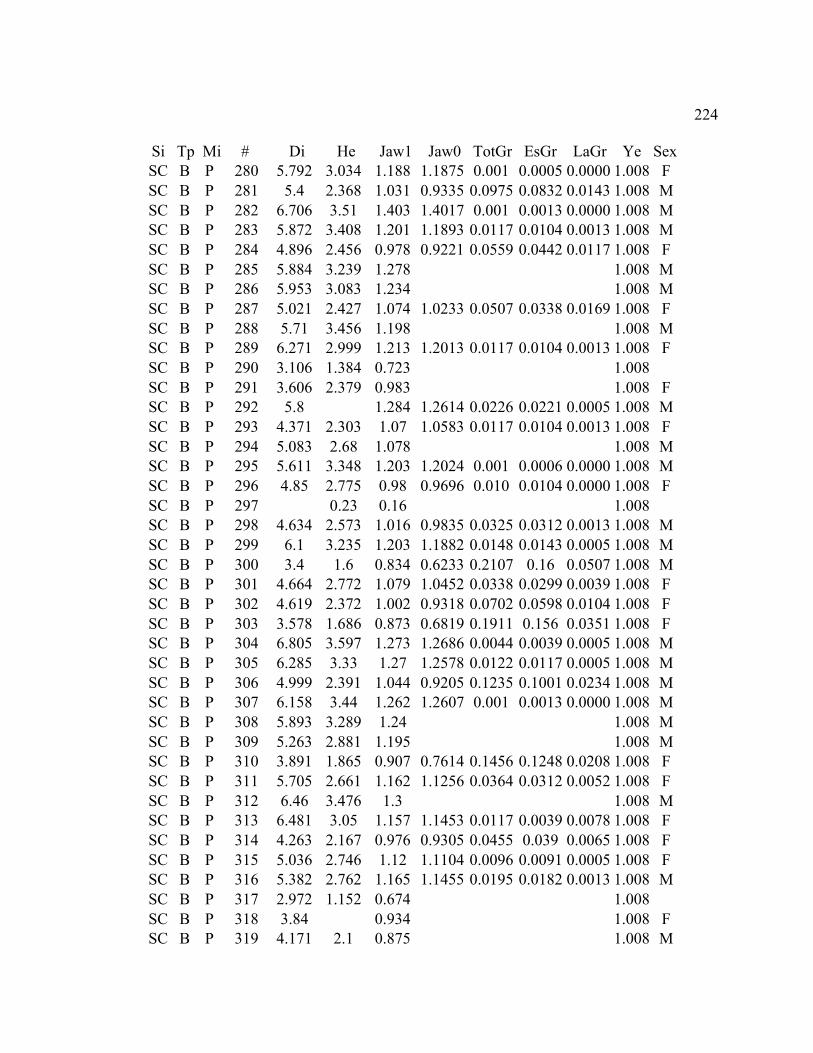
224
Si Tp Mi # Di He Jaw1 Jaw0 TotGr EsGr LaGr Ye Sex
SC B P 280 5.792 3.034 1.188 1.1875 0.001 0.0005 0.0000 1.008 F
SC B P 281 5.4 2.368 1.031 0.9335 0.0975 0.0832 0.0143 1.008 M
SC B P 282 6.706 3.51 1.403 1.4017 0.001 0.0013 0.0000 1.008 M
SC B P 283 5.872 3.408 1.201 1.1893 0.0117 0.0104 0.0013 1.008 M
SC B P 284 4.896 2.456 0.978 0.9221 0.0559 0.0442 0.0117 1.008 F
SC B P 285 5.884 3.239 1.278 1.008 M
SC B P 286 5.953 3.083 1.234 1.008 M
SC B P 287 5.021 2.427 1.074 1.0233 0.0507 0.0338 0.0169 1.008 F
SC B P 288 5.71 3.456 1.198 1.008 M
SC B P 289 6.271 2.999 1.213 1.2013 0.0117 0.0104 0.0013 1.008 F
SC B P 290 3.106 1.384 0.723 1.008
SC B P 291 3.606 2.379 0.983 1.008 F
SC B P 292 5.8 1.284 1.2614 0.0226 0.0221 0.0005 1.008 M
SC B P 293 4.371 2.303 1.07 1.0583 0.0117 0.0104 0.0013 1.008 F
SC B P 294 5.083 2.68 1.078 1.008 M
SC B P 295 5.611 3.348 1.203 1.2024 0.001 0.0006 0.0000 1.008 M
SC B P 296 4.85 2.775 0.98 0.9696 0.010 0.0104 0.0000 1.008 F
SC B P 297 0.23 0.16 1.008
SC B P 298 4.634 2.573 1.016 0.9835 0.0325 0.0312 0.0013 1.008 M
SC B P 299 6.1 3.235 1.203 1.1882 0.0148 0.0143 0.0005 1.008 M
SC B P 300 3.4 1.6 0.834 0.6233 0.2107 0.16 0.0507 1.008 M
SC B P 301 4.664 2.772 1.079 1.0452 0.0338 0.0299 0.0039 1.008 F
SC B P 302 4.619 2.372 1.002 0.9318 0.0702 0.0598 0.0104 1.008 F
SC B P 303 3.578 1.686 0.873 0.6819 0.1911 0.156 0.0351 1.008 F
SC B P 304 6.805 3.597 1.273 1.2686 0.0044 0.0039 0.0005 1.008 M
SC B P 305 6.285 3.33 1.27 1.2578 0.0122 0.0117 0.0005 1.008 M
SC B P 306 4.999 2.391 1.044 0.9205 0.1235 0.1001 0.0234 1.008 M
SC B P 307 6.158 3.44 1.262 1.2607 0.001 0.0013 0.0000 1.008 M
SC B P 308 5.893 3.289 1.24 1.008 M
SC B P 309 5.263 2.881 1.195 1.008 M
SC B P 310 3.891 1.865 0.907 0.7614 0.1456 0.1248 0.0208 1.008 F
SC B P 311 5.705 2.661 1.162 1.1256 0.0364 0.0312 0.0052 1.008 F
SC B P 312 6.46 3.476 1.3 1.008 M
SC B P 313 6.481 3.05 1.157 1.1453 0.0117 0.0039 0.0078 1.008 F
SC B P 314 4.263 2.167 0.976 0.9305 0.0455 0.039 0.0065 1.008 F
SC B P 315 5.036 2.746 1.12 1.1104 0.0096 0.0091 0.0005 1.008 F
SC B P 316 5.382 2.762 1.165 1.1455 0.0195 0.0182 0.0013 1.008 M
SC B P 317 2.972 1.152 0.674 1.008
SC B P 318 3.84 0.934 1.008 F
SC B P 319 4.171 2.1 0.875 1.008 M

225
Si Tp Mi # Di He Jaw1 Jaw0 TotGr EsGr LaGr Ye Sex
SC B P 320 5.777 3.284 1.222 1.008 M
SC B NP 321 6.628 3.757 1.241 1.008 M
SC B NP 322 6.282 3.839 1.335 1.3272 0.008 0.0078 0.0000 1.008 F
SC B NP 323 4.85 2.404 1.043 0.9702 0.0728 0.0676 0.0052 1.008 F
SC B NP 324 7.809 3.948 1.4 1.008 M
SC B NP 325 6.454 3.426 1.241 1.2327 0.0083 0.0078 0.0005 1.008 F
SC B NP 326 6.772 3.63 1.32 1.3187 0.001 0.0013 0.0000 1.008 M
SC B NP 327 4.992 2.259 0.945 0.9008 0.0442 0.0364 0.0078 1.008 F
SC B NP 328 3.6 1.9 0.85 0.7694 0.0806 0.0676 0.0130 1.008 F
SC B NP 329 6.267 3.28 1.204 1.1637 0.0403 0.0351 0.0052 1.008 F
SC B NP 330 6.054 3.199 1.119 1.0904 0.0286 0.026 0.0026 1.008 M
SC B NP 331 5.985 3.311 1.17 1.008 M
SC B NP 332 3.63 1.511 0.766 1.008 F
SC B NP 333 4.66 2.197 0.955 1.008 M
SC B NP 334 3.82 2.079 0.877 1.008 F
SC B NP 335 7.224 4.179 1.308 1.008 M
SC B NP 336 7.718 3.823 1.528 1.008 M
SC B NP 337 0.82 0.333 0.216 1.008
SC B NP 338 6.327 2.993 1.268 1.008 F
SC B NP 339 4.5 2.303 0.966 1.008 M
SC B NP 340 6.83 3.165 1.253 1.008 M
SC B NP 341 3.682 1.609 0.783 1.008 M
SC B NP 342 5.657 3.515 1.154 1.008 F
SC B NP 343 2.877 1.514 0.718 0.5329 0.1851 0.15 0.0351 1.008 F
SC B NP 344 7.125 3.521 1.337 1.3331 0.0039 0.0026 0.0013 1.008 M
SC B NP 345 6.133 3.202 1.221 1.2153 0.0057 0.0052 0.0005 1.008 F
SC B NP 346 6.512 3.513 1.136 1.008 M
SC B NP 347 4.167 0.892 0.7438 0.1482 0.1157 0.0325 1.008 F
SC B NP 348 6.03 3.133 1.375 1.362 0.013 0.0052 0.0078 1.008 M
SC B NP 349 6.289 3.26 1.216 1.008 M
SC B NP 350 6.792 3.73 1.304 1.2949 0.0091 0.0039 0.0052 1.008 F
SC B NP 351 2.714 1.198 0.574 1.008
SC B NP 352 1.689 0.702 0.393 1.008
SC B NP 353 1.453 0.66 0.369 1.008
SC C P 354 6.12 3.45 1.264 1.000 M
SC C P 355 5.79 2.93 1.126 1.1195 0.0065 0.0052 0.0013 1.000 F
SC C P 356 6.146 3.226 1.231 1.000 F
SC C P 357 4.958 2.623 1.09 1.000 M
SC C P 358 4.81 1.033 1.000 F
SC C P 359 5.049 2.853 1.064 1.000 F
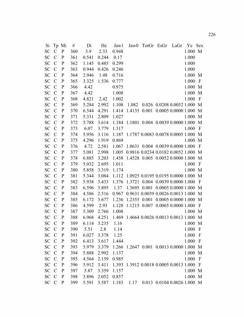
226
Si Tp Mi # Di He Jaw1 Jaw0 TotGr EsGr LaGr Ye Sex
SC C P 360 3.9 2.33 0.948 1.000 M
SC C P 361 0.541 0.244 0.17 1.000
SC C P 362 1.145 0.485 0.299 1.000
SC C P 363 0.944 0.426 0.246 1.000
SC C P 364 2.946 1.48 0.716 1.000 M
SC C P 365 3.325 1.536 0.777 1.000 F
SC C P 366 4.42 0.975 1.000 M
SC C P 367 4.42 1.008 1.000 M
SC C P 368 4.821 2.42 1.002 1.000 F
SC C P 369 5.284 2.992 1.108 1.082 0.026 0.0208 0.0052 1.000 M
SC C P 370 6.544 4.291 1.414 1.4135 0.001 0.0005 0.0000 1.000 M
SC C P 371 5.331 2.809 1.027 1.000 M
SC C P 372 5.788 3.614 1.184 1.1801 0.004 0.0039 0.0000 1.000 M
SC C P 373 6.07 3.779 1.317 1.000 F
SC C P 374 5.956 3.116 1.187 1.1787 0.0083 0.0078 0.0005 1.000 M
SC C P 375 4.296 1.919 0.869 1.000 M
SC C P 376 4.72 2.581 1.067 1.0631 0.004 0.0039 0.0000 1.000 F
SC C P 377 5.081 2.998 1.005 0.9816 0.0234 0.0182 0.0052 1.000 M
SC C P 378 6.885 3.203 1.458 1.4528 0.005 0.0052 0.0000 1.000 M
SC C P 379 5.032 2.695 1.011 1.000 F
SC C P 380 5.858 3.319 1.174 1.000 M
SC C P 381 5.344 3.084 1.112 1.0925 0.0195 0.0195 0.0000 1.000 M
SC C P 382 5.938 3.433 1.376 1.3721 0.004 0.0039 0.0000 1.000 F
SC C P 383 6.596 3.895 1.37 1.3695 0.001 0.0005 0.0000 1.000 M
SC C P 384 4.586 2.516 0.967 0.9631 0.0039 0.0026 0.0013 1.000 M
SC C P 385 6.172 3.677 1.236 1.2355 0.001 0.0005 0.0000 1.000 M
SC C P 386 4.599 2.93 1.128 1.1215 0.007 0.0065 0.0000 1.000 F
SC C P 387 5.309 2.766 1.008 1.000 M
SC C P 388 6.968 4.251 1.469 1.4664 0.0026 0.0013 0.0013 1.000 M
SC C P 389 6.114 3.235 1.16 1.000 M
SC C P 390 5.51 2.8 1.14 1.000 F
SC C P 391 6.027 3.378 1.25 1.000 F
SC C P 392 6.413 3.617 1.444 1.000 F
SC C P 393 5.979 3.379 1.266 1.2647 0.001 0.0013 0.0000 1.000 M
SC C P 394 5.888 2.992 1.137 1.000 M
SC C P 395 4.564 2.159 0.985 1.000 F
SC C P 396 5.912 3.411 1.393 1.3912 0.0018 0.0005 0.0013 1.000 F
SC C P 397 5.87 3.359 1.157 1.000 M
SC C P 398 3.896 2.052 0.857 1.000 M
SC C P 399 5.591 3.587 1.183 1.17 0.013 0.0104 0.0026 1.000 M
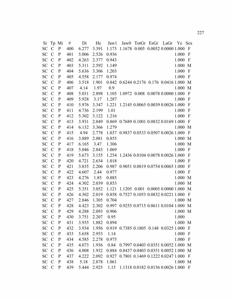
227
Si Tp Mi # Di He Jaw1 Jaw0 TotGr EsGr LaGr Ye Sex
SC C P 400 6.277 3.391 1.173 1.1678 0.005 0.0052 0.0000 1.000 F
SC C P 401 5.006 2.526 0.936 1.000 F
SC C P 402 4.263 2.377 0.943 1.000 F
SC C P 403 5.311 2.592 1.149 1.000 M
SC C P 404 5.636 3.306 1.203 1.000 F
SC C P 405 4.558 2.177 0.974 1.000 F
SC C P 406 3.518 1.901 0.842 0.6244 0.2176 0.176 0.0416 1.000 M
SC C P 407 4.14 1.97 0.9 1.000 M
SC C P 408 5.031 2.898 1.105 1.0972 0.008 0.0078 0.0000 1.000 F
SC C P 409 5.928 3.17 1.287 1.000 F
SC C P 410 5.976 3.347 1.221 1.2145 0.0065 0.0039 0.0026 1.000 F
SC C P 411 4.736 2.199 1.01 1.000 F
SC C P 412 5.302 3.122 1.216 1.000 F
SC C P 413 3.931 2.049 0.869 0.7689 0.1001 0.0832 0.0169 1.000 F
SC C P 414 6.132 3.366 1.279 1.000 M
SC C P 415 4.94 2.778 1.037 0.9837 0.0533 0.0507 0.0026 1.000 F
SC C P 416 3.889 2.081 0.855 1.000 M
SC C P 417 6.165 3.47 1.306 1.000 M
SC C P 418 5.046 2.843 1.069 1.000 F
SC C P 419 5.673 3.155 1.254 1.2436 0.0104 0.0078 0.0026 1.000 F
SC C P 420 4.721 2.634 1.018 1.000 F
SC C P 421 3.835 2.206 0.987 0.9051 0.0819 0.0754 0.0065 1.000 F
SC C P 422 4.607 2.44 0.977 1.000 F
SC C P 423 4.276 1.85 0.885 1.000 M
SC C P 424 4.302 2.039 0.853 1.000 M
SC C P 425 5.351 3.052 1.121 1.1205 0.001 0.0005 0.0000 1.000 M
SC C P 426 4.302 2.019 0.858 0.7527 0.1053 0.0832 0.0221 1.000 F
SC C P 427 2.846 1.305 0.704 1.000 M
SC C P 428 4.423 2.302 0.997 0.9255 0.0715 0.0611 0.0104 1.000 M
SC C P 429 4.288 2.093 0.906 1.000 M
SC C P 430 3.751 2.207 0.95 1.000
SC C P 431 3.935 1.882 0.894 1.000 M
SC C P 432 3.934 1.956 0.919 0.7385 0.1805 0.148 0.0325 1.000 F
SC C P 433 5.658 2.953 1.14 1.000 F
SC C P 434 4.585 2.278 0.975 1.000 F
SC C P 435 4.073 1.936 0.84 0.7997 0.0403 0.0351 0.0052 1.000 M
SC C P 436 4.008 1.932 0.884 0.8437 0.0403 0.0351 0.0052 1.000 M
SC C P 437 4.222 2.092 0.927 0.7801 0.1469 0.1222 0.0247 1.000 F
SC C P 438 5.18 2.878 1.061 1.000 M
SC C P 439 5.444 2.925 1.15 1.1318 0.0182 0.0156 0.0026 1.000 F
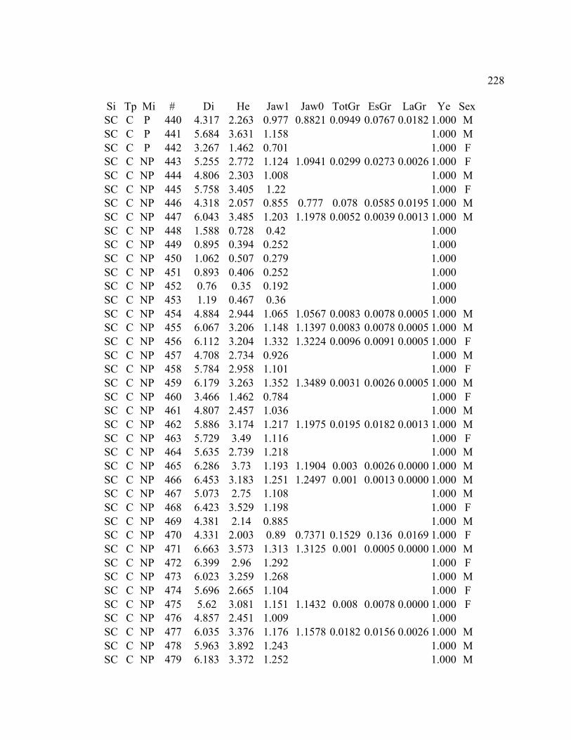
228
Si Tp Mi # Di He Jaw1 Jaw0 TotGr EsGr LaGr Ye Sex
SC C P 440 4.317 2.263 0.977 0.8821 0.0949 0.0767 0.0182 1.000 M
SC C P 441 5.684 3.631 1.158 1.000 M
SC C P 442 3.267 1.462 0.701 1.000 F
SC C NP 443 5.255 2.772 1.124 1.0941 0.0299 0.0273 0.0026 1.000 F
SC C NP 444 4.806 2.303 1.008 1.000 M
SC C NP 445 5.758 3.405 1.22 1.000 F
SC C NP 446 4.318 2.057 0.855 0.777 0.078 0.0585 0.0195 1.000 M
SC C NP 447 6.043 3.485 1.203 1.1978 0.0052 0.0039 0.0013 1.000 M
SC C NP 448 1.588 0.728 0.42 1.000
SC C NP 449 0.895 0.394 0.252 1.000
SC C NP 450 1.062 0.507 0.279 1.000
SC C NP 451 0.893 0.406 0.252 1.000
SC C NP 452 0.76 0.35 0.192 1.000
SC C NP 453 1.19 0.467 0.36 1.000
SC C NP 454 4.884 2.944 1.065 1.0567 0.0083 0.0078 0.0005 1.000 M
SC C NP 455 6.067 3.206 1.148 1.1397 0.0083 0.0078 0.0005 1.000 M
SC C NP 456 6.112 3.204 1.332 1.3224 0.0096 0.0091 0.0005 1.000 F
SC C NP 457 4.708 2.734 0.926 1.000 M
SC C NP 458 5.784 2.958 1.101 1.000 F
SC C NP 459 6.179 3.263 1.352 1.3489 0.0031 0.0026 0.0005 1.000 M
SC C NP 460 3.466 1.462 0.784 1.000 F
SC C NP 461 4.807 2.457 1.036 1.000 M
SC C NP 462 5.886 3.174 1.217 1.1975 0.0195 0.0182 0.0013 1.000 M
SC C NP 463 5.729 3.49 1.116 1.000 F
SC C NP 464 5.635 2.739 1.218 1.000 M
SC C NP 465 6.286 3.73 1.193 1.1904 0.003 0.0026 0.0000 1.000 M
SC C NP 466 6.453 3.183 1.251 1.2497 0.001 0.0013 0.0000 1.000 M
SC C NP 467 5.073 2.75 1.108 1.000 M
SC C NP 468 6.423 3.529 1.198 1.000 F
SC C NP 469 4.381 2.14 0.885 1.000 M
SC C NP 470 4.331 2.003 0.89 0.7371 0.1529 0.136 0.0169 1.000 F
SC C NP 471 6.663 3.573 1.313 1.3125 0.001 0.0005 0.0000 1.000 M
SC C NP 472 6.399 2.96 1.292 1.000 F
SC C NP 473 6.023 3.259 1.268 1.000 M
SC C NP 474 5.696 2.665 1.104 1.000 F
SC C NP 475 5.62 3.081 1.151 1.1432 0.008 0.0078 0.0000 1.000 F
SC C NP 476 4.857 2.451 1.009 1.000
SC C NP 477 6.035 3.376 1.176 1.1578 0.0182 0.0156 0.0026 1.000 M
SC C NP 478 5.963 3.892 1.243 1.000 M
SC C NP 479 6.183 3.372 1.252 1.000 M
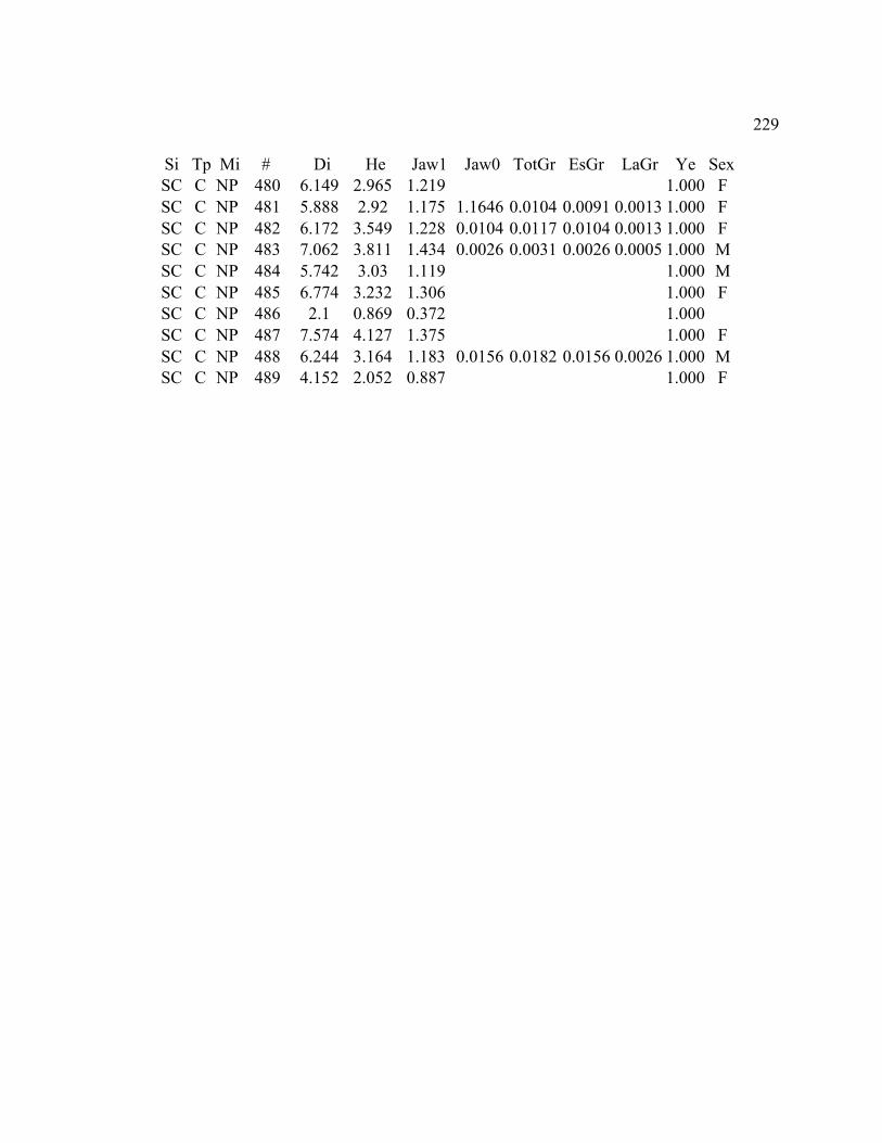
229
Si Tp Mi # Di He Jaw1 Jaw0 TotGr EsGr LaGr Ye Sex
SC C NP 480 6.149 2.965 1.219 1.000 F
SC C NP 481 5.888 2.92 1.175 1.1646 0.0104 0.0091 0.0013 1.000 F
SC C NP 482 6.172 3.549 1.228 0.0104 0.0117 0.0104 0.0013 1.000 F
SC C NP 483 7.062 3.811 1.434 0.0026 0.0031 0.0026 0.0005 1.000 M
SC C NP 484 5.742 3.03 1.119 1.000 M
SC C NP 485 6.774 3.232 1.306 1.000 F
SC C NP 486 2.1 0.869 0.372 1.000
SC C NP 487 7.574 4.127 1.375 1.000 F
SC C NP 488 6.244 3.164 1.183 0.0156 0.0182 0.0156 0.0026 1.000 M
SC C NP 489 4.152 2.052 0.887 1.000 F

230
APPENDIX D
SEA URCHIN PREDATION DATA
These data collected from the East Side of South Cove, Cape Arago are
summarized in Fig. 5 and Fig. 6 in Chapter V. All data are measurements of test diameter
(cm) from live sea urchins, dead sea urchins eaten by black oystercatchers (BLOY), and
dead sea urchins eaten by raccoons. Fig. 1 in Chapter V displays the different areas of the
East Side referred to as the Boulder Field, Sandstone Benches, Low Islands, and Sandy,
Protected area.
Live Sea Urchins
Boulder Field
Quadrat 1
7.0
3.8
6.7
3.7
5.1
5.5
4.0
5.7
4.8
4.9
5.6
4.3
5.8
5.8
5.3
4.6
5.2
6.6
5.4
5.8
5.9
2.8
6.7
7.9
7.0
5.6
5.7
5.2
3.6
3.7
5.5
3.9
5.3
5.4
6.6
5.7
5.6
6.2
5.4
7.3
6.6
4.4
7.6
Quadrat 2
6.6
4.8
4.3
5.4
6.1
4.2
5.3
4.6
5.6
4.2
4.0
4.7
4.0
4.3
3.4
6.2
4.8
4.8
5.5
5.9
5.3
6.6
4.3
5.7
6.8
5.9
4.4
5.3
6.2
5.7
3.8
6.1
5.0
6.4
4.3
5.4
5.5
4.4
6.4
3.0
5.3
5.2
6.0
6.0
4.1
5.8
4.9
5.2
5.6
4.7
6.7
6.7
5.2
5.5
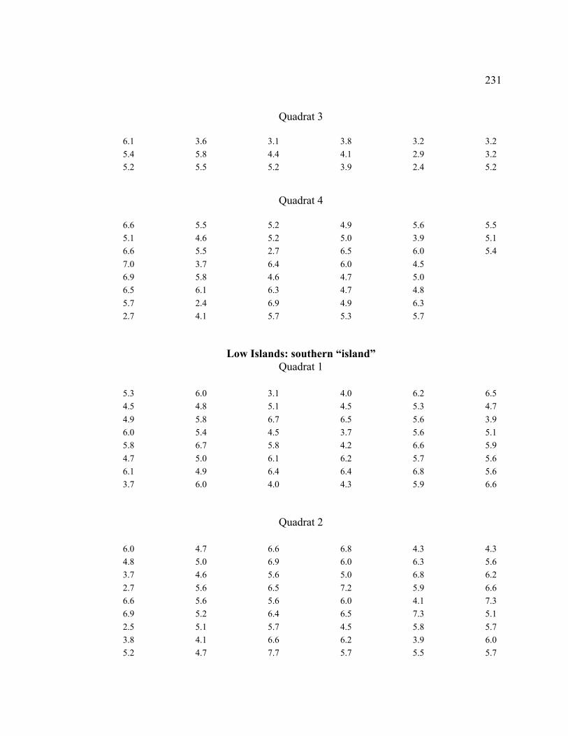
231
Quadrat 3
6.1
5.4
5.2
3.6
5.8
5.5
3.1
4.4
5.2
3.8
4.1
3.9
3.2
2.9
2.4
3.2
3.2
5.2
Quadrat 4
6.6
5.1
6.6
7.0
6.9
6.5
5.7
2.7
5.5
4.6
5.5
3.7
5.8
6.1
2.4
4.1
5.2
5.2
2.7
6.4
4.6
6.3
6.9
5.7
4.9
5.0
6.5
6.0
4.7
4.7
4.9
5.3
5.6
3.9
6.0
4.5
5.0
4.8
6.3
5.7
5.5
5.1
5.4
Low Islands: southern “island”
Quadrat 1
5.3
4.5
4.9
6.0
5.8
4.7
6.1
3.7
6.0
4.8
5.8
5.4
6.7
5.0
4.9
6.0
3.1
5.1
6.7
4.5
5.8
6.1
6.4
4.0
4.0
4.5
6.5
3.7
4.2
6.2
6.4
4.3
6.2
5.3
5.6
5.6
6.6
5.7
6.8
5.9
6.5
4.7
3.9
5.1
5.9
5.6
5.6
6.6
Quadrat 2
6.0
4.8
3.7
2.7
6.6
6.9
2.5
3.8
5.2
4.7
5.0
4.6
5.6
5.6
5.2
5.1
4.1
4.7
6.6
6.9
5.6
6.5
5.6
6.4
5.7
6.6
7.7
6.8
6.0
5.0
7.2
6.0
6.5
4.5
6.2
5.7
4.3
6.3
6.8
5.9
4.1
7.3
5.8
3.9
5.5
4.3
5.6
6.2
6.6
7.3
5.1
5.7
6.0
5.7

232
4.4 4.3
Quadrat 3
7.1
5.5
6.2
6.7
7.3
5.4
5.5
4.6
5.3
6.3
4.6
4.9
5.2
6.3
5.1
4.8
6.4
1.5
6.5
4.1
4.1
5.3
5.6
4.2
5.5
5.7
5.1
5.1
6.7
5.7
5.2
6.7
4.0
3.5
3.7
4.8
5.3
4.3
4.5
4.1
5.2
3.9
4.2
5.9
5.1
Quadrat 4
6.3
5.9
5.9
5.3
6.3
5.4
5.8
5.8
4.3
6.2
5.9
6.8
4.9
5.1
6.0
1.9
3.9
6.0
5.6
4.9
5.5
6.1
4.0
5.3
6.7
2.6
5.0
5.9
5.6
6.8
6.6
6.1
5.5
4.3
2.8
4.2
6.1
6.7
5.9
4.9
5.4
5.7
4.9
4.0
Low Islands: northern “island”
Quadrat 1
3.9
6.6
5.4
5.8
6.4
5.5
4.8
3.7
1.8
7.4
2.9
4.8
6.5
5.3
3.8
4.5
2.7
6.0
5.3
5.7
5.1
5.6
4.2
3.7
4.1
6.8
4.3
4.2
6.3
4.0
3.2
6.7
4.7
5.3
6.2
7.0
6.4
4.3
4.5
4.1
5.3
5.5
5.3
6.4
6.8
4.0
6.2
4.9
5.2
4.8

233
Quadrat 2
6.2
5.8
4.9
6.5
6.2
5.9
3.2
3.1
5.3
5.4
4.4
4.6
5.6
5.2
4.7
5.8
5.3
5.4
5.1
6.1
5.9
6.2
4.8
3.7
2.8
5.7
5.5
4.4
5.2
6.7
4.6
5.1
5.2
4.2
5.3
4.8
5.1
4.5
6.4
6.6
4.6
5.0
6.0
6.5
5.4
3.9
5.2
5.7
4.6
6.2
6.5
5.9
5.4
5.0
4.1
7.1
4.9
6.7
6.1
5.4
Quadrat 3
5.8
4.5
4.4
6.0
4.7
6.1
5.7
5.5
5.6
4.6
5.3
4.6
4.6
4.4
5.6
5.1
6.4
6.1
5.9
3.2
4.5
3.0
4.7
4.0
4.6
6.5
6.0
4.7
4.0
5.0
5.4
5.1
2.3
6.0
5.1
4.2
4.9
5.9
4.4
4.8
5.0
4.9
5.5
4.9
5.7
4.9
5.7
5.5
5.4
6.3
4.8
6.7
4.9
3.6
6.0
5.5
5.3
6.1
5.9
5.2
4.7
4.3
5.7
4.5
Quadrat 4
4.4
1.7
5.9
6.0
3.8
6.1
6.5
5.5
3.8
5.2
4.6
4.5
5.6
3.2
3.3
5.1
4.4
4.9
6.5
4.1
3.9
6.2
5.7
3.1
3.7
4.3
5.3
3.5
5.3
5.9
4.5
5.9
3.0
6.9
5.6
4.4
5.8
3.6
6.6
4.4
3.5
3.4
7.0
5.2
5.8
5.4
4.0
5.3
5.1
4.5
6.0
5.9
3.0
6.6
5.1
5.4
4.3
3.4
4.7
5.2
5.7
6.5
3.8
6.2
5.8

234
Quadrat 5
7.0
5.7
4.7
4.1
5.0
5.9
4.1
5.6
5.9
5.7
4.4
5.6
4.6
5.1
6.1
5.0
5.6
3.5
3.6
5.3
4.4
5.9
6.0
4.7
6.1
5.7
5.5
5.6
5.4
6.6
4.2
4.9
6.9
4.4
4.2
5.4
2.8
5.1
3.3
3.7
3.4
3.0
6.1
4.4
4.3
5.6
4.5
5.8
4.5
5.9
5.5
6.5
5.0
6.6
6.2
6.7
5.3
5.6
5.9
5.1
5.9
5.9
4.1
4.8
6.2
5.2
5.6
4.7
4.7
5.3
5.6
Sandstone Benches
Quadrat 1
6.7
6.3
6.0
7.3
6.8
5.7
6.4
3.6
6.3
5.8
5.5
6.5
4.7
5.4
6.7
6.1
6.4
6.8
7.2
3.9
5.6
5.1
5.1
5.1
3.5
7.3
6.2
6.9
5.3
6.3
6.3
6.5
Quadrat 2
5.7
5.9
5.9
5.5
5.4
4.3
6.0
6.0
6.1
7.3
7.3
7.2
5.1
Quadrat 3
5.3
4.2
3.9
3.1
4.9
2.9
4.5
3.7
4.0
2.9
3.7
3.7
3.0
4.3
4.1
4.1
4.3
4.8
4.7
4.6
1.1
4.6
4.4
3.8
3.7
3.4
3.6
3.9
3.8
4.0
3.8
5.4
4.5
3.7
4.7
4.5
3.9
235
Quadrat 4
5.0
4.4
6.6
4.3
5.7
4.9
4.3
4.6
5.3
5.1
5.6
5.7
5.2
5.7
6.3
5.9
5.5
6.0
5.6
6.1
5.9
5.8
6.4
6.0
3.6
3.9
6.1
5.4
Quadrat 5
4.0
5.1
3.6
4.0
4.2
5.0
5.5
5.1
4.4
4.7
5.2
3.8
2.9
4.9
4.6
4.5
4.7
3.4
4.5
2.6
6.5
5.3
5.8
5.0
4.2
5.2
4.1
5.2
3.0
4.0
4.4
4.0
6.7
5.3
6.5
Quadrat 6
7.9
6.6
5.6
4.9
7.7
5.8
6.4
5.4
7.0
6.9
5.0
6.9
4.9
5.4
5.8
6.7
6.8
7.9
6.7
7.1
6.9
4.8
6.1
4.3
3.7
5.1
5.9
4.8
7.5
5.7
7.3
6.3
4.6
6.9
5.0
6.4
6.1
5.3
6.4
7.6
5.1
6.4
7.0
6.0
6.1
6.4
4.3
6.2
Quadrat 7
7.0
6.8
4.5
7.0
5.0
7.4
7.1
6.0
6.4
7.3
6.9
6.7
4.2
6.0
6.9
3.9
5.8
6.1
7.0
2.0
4.4
6.7
6.7
4.3
6.8
4.7
6.7
4.4
7.5
6.9
4.3
7.4
7.2
Quadrat 8
6.9 6.9 6.9 7.2 7.2 7.5
236
6.0
6.2
7.1
7.6
7.8
6.9
7.2
7.1
5.0
5.4
7.8
6.1
6.2
6.7
6.8
6.3
6.4
4.8
5.4
5.9
7.9
7.3
8.3
5.8
7.0
7.5
5.3
4.7
5.5
8.0
7.8
7.4
7.1
7.2
7.2
6.9
8.4
7.4
7.3
6.9
5.6
6.7
Quadrat 9
6.3
6.2
2.3
4.9
6.5
6.7
7.0
6.8
6.8
5.2
7.0
7.6
3.4
1.9
5.9
6.5
6.7
6.7
6.7
6.5
6.1
6.2
7.0
7.1
6.4
6.3
6.6
6.5
6.4
4.0
5.6
7.1
6.8
5.1
6.6
6.5
6.6
5.6
6.5
6.8
6.9
6.6
7.5
5.7
5.9
5.0
5.0
5.1
5.3
7.7
5.3
5.8
6.9
6.5
5.8
7.4
5.4
5.5
5.6
6.5
6.9
4.2
6.4
6.3
6.6
6.6
5.4
5.1
7.2
6.9
6.6
6.7
6.4
2.7
5.6
7.3
5.9
6.2
6.3
6.5
4.6
5.4
6.0
6.6
Sandstone Benches: eastern side
Quadrat 1
5.9
4.9
6.4
6.3
5.4
5.5
4.2
6.7
5.8
5.6
5.2
5.5
4.9
6.5
5.1
5.4
4.2
4.3
4.4
6.4
5.4
6.5
5.7
4.5
4.6
6.7
4.2
4.1
5.7
5.7
Quadrat 2
5.6
5.5
4.9
5.8
5.7
6.2
4.9
5.4
6.2
5.7
6.3
5.8
5.9
6.2
6.2
6.7
4.7
6.5
5.8
6.4
5.4
6.6
6.0
5.9
5.4
5.9
6.5
6.2
6.1
4.1

237
2.6
6.1
6.5
5.5
7.5
6.1
7.0
4.5
4.6
5.3
4.8
2.7
5.7
Quadrat 3
5.9
5.7
5.9
3.6
6.5
5.8
7.4
6.8
5.2
5.8
6.8
7.1
6.2
5.2
6.5
6.5
5.9
3.4
4.9
7.5
6.6
6.2
2.3
6.2
3.5
5.9
6.6
5.6
6.2
5.0
6.4
5.5
6.6
4.2
6.5
5.8
5.3
4.6
6.5
6.4
6.6
4.5
6.8
4.1
5.7
4.9
6.1
3.3
7.3
Sea Urchins Eaten by Oystercatchers
Low Islands: southern “island”
7.3
7.7
6.2
6.3
7.2
6.3
6.4
5.7
7.5
6.3
6.4
6.9
6.1
6.0
7.2
7.2
6.0
6.3
6.4
6.5
6.5
6.8
6.3
5.9
6.6
6.8
7.2
7.5
6.6
6.4
7.3
6.4
5.8
6.2
6.3
6.4
6.4
6.8
6.9
7.1
6.4
6.5
5.4
6.9
7.1
6.8
6.1
Low Islands: northern “island”
7.0
6.4
6.3
5.7
6.4
6.7
6.0
6.4
6.0
6.3
6.0
5.7
6.5
6.7
6.1
5.7
7.5
7.4
6.3
7.0
5.7
5.7
6.6
7.0
7.0
5.3
6.7
5.4
6.4
7.2
7.5
6.2
7.2
238
Sandstone Benches
7.2
6.1
6.3
6.5
6.2
6.9
7.0
6.6
7.4
7.3
7.9
7.1
7.0
6.4
7.1
7.3
7.3
6.6
6.7
7.6
7.1
7.7
7.5
6.5
5.3
6.9
6.4
6.4
6.5
7.4
5.3
7.3
6.5
6.2
6.8
6.2
5.8
7.6
7.4
6.1
6.1
6.4
6.7
6.9
6.6
6.3
5.2
6.8
6.6
6.7
9.0
6.7
8.0
7.6
5.6
6.9
7.9
7.1
6.2
7.2
6.9
6.7
5.1
6.7
6.5
6.8
6.3
6.7
6.4
5.6
7.1
7.1
7.1
7.5
6.5
6.7
6.7
6.8
6.4
7.3
6.9
6.5
7.4
6.8
6.0
6.5
5.6
6.0
6.3
6.3
6.6
6.8
7.0
7.5
6.8
5.4
6.8
6.9
7.1
7.3
5.6
6.1
6.7
6.9
6.7
7.2
7.9
6.0
6.2
6.5
5.3
6.2
6.3
6.9
7.2
6.7
7.6
7.5
6.7
6.6
7.3
5.7
6.8
6.8
6.3
5.9
6.8
7.1
7.0
6.0
6.3
5.5
7.5
8.2
5.9
6.6
7.1
7.6
6.8
5.2
6.3
6.4
5.7
5.7
Sandstone Benches: eastern side
7.0
7.1
6.5
7.4
6.4
6.0
6.6
5.9
5.9
6.0
6.6
7.0
5.9
5.8
6.1
6.6
6.3
5.8
7.2
6.1
7.0
6.9
7.0
7.5
Sandy, Protected Area
6.9
8.0
7.8
7.4
7.1
7.8
7.5
7.7
6.3
5.1
7.7
7.6
6.4
6.7
6.5
6.6
6.9
7.4
6.9
8.5
5.5
5.9
6.1
7.1
7.4
6.5
6.8
6.8
7.2
8.0
239
8.2
6.7
6.8
7.7
8.1
8.0
7.4
7.2
7.0
7.4
5.8
6.6
8.4
7.9
6.9
5.5
5.8
7.1
7.4
7.5
4.5
5.7
6.0
6.2
4.5
6.9
6.7
7.7
8.8
5.6
7.4
6.7
7.6
6.9
8.3
7.4
6.3
6.8
7.4
9.1
8.6
6.1
6.8
7.1
5.1
Dead Sea Urchins Eaten by Raccoons
Boulder Field
6.9
7.5
7.4
7.6
7.5
7.0
7.3
8.6
6.2
6.8
7.3
6.6
8.0
7.3
8.5
8.3
6.9
7.5
7.6
7.2
7.9
8.6
7.6
7.3
7.4
7.4
7.4
6.5
9.3
7.9
7.6
7.9
7.0
7.2
7.4
8.0
8.0
8.0
8.2
8.3
6.9
8.2
6.5
7.4
7.4
7.6
7.8
7.0
6.7
6.5
7.9
8.0
6.6
7.0
6.6
7.8
7.0
7.1
7.8
7.0
6.9
7.5
7.1
7.1
6.3
7.5
6.9
7.3
7.6
8.1
7.3
7.8
6.7
6.7
8.0
7.2
8.0
8.6
8.0
8.2
7.3
7.5
6.9
8.6
8.0
7.7
7.8
6.9
7.2
8.4
6.9
7.9
6.7
6.9
7.6
8.6
7.4
7.6
8.6
7.4
7.9
7.8
7.1
8.1
7.6
6.9
8.0
7.4
7.9
8.1
8.3
6.9
7.1
6.4
6.8
7.0
7.0
7.9
8.0
7.8
6.0
6.2
6.7
8.3
6.4
7.4
7.6
7.7
7.7
6.6
7.1
7.4
6.5
6.5
7.1
7.7
6.1
8.0
7.1
6.3
5.5
7.4
6.6
6.5
8.0
7.5
6.8
6.5
6.7
7.1
7.5
6.3
6.7
7.1
7.5
6.4
9.1
7.2
6.5
5.7
6.1
6.8
7.5
7.5
6.4
6.6
5.8
6.6
240
7.6
6.4
6.8
7.4
6.8
6.6
6.7
7.7
7.1
6.8
6.8
7.1
7.6
6.6
7.0
6.4
5.9
6.5
7.0
6.1
7.1
6.7
6.6
6.6
6.6
6.5
7.8
6.1
6.1
6.2
6.4
5.1
6.6
6.6
6.6
7.3
7.3
5.3
8.0
6.1
7.7
7.7
6.9
7.5
6.9
8.0
5.1
7.7
8.1
5.3
7.2
8.2
8.4
7.2
4.9
7.6
6.8
7.2
6.7
6.5
7.0
6.9
6.7
6.6
8.2
7.4
7.9
7.9
7.0
7.4
6.6
7.5
8.3
8.6
7.0
6.5
7.6
7.5
7.4
7.2
7.2
7.6
7.9
6.7
6.4
8.2
7.0
6.7
7.2
8.2
7.5
8.3
8.1
8.2
8.0
7.5
7.2
8.2
6.5
6.8
6.9
7.4
7.5
8.8
7.2
7.4
7.5
8.4
7.4
8.2
6.2
5.8
5.4
6.0
6.3
5.6
7.3
7.2
7.2
8.2
8.2
9.1
5.6
7.2
7.5
8.6
6.4
7.9
7.5
6.4
6.3
6.2
6.6
7.3
6.0
6.2
6.8
5.1
6.0
6.0
6.7
5.3
7.2
6.6
7.4
7.2
6.5
7.7
7.4
6.9
6.9
5.5
6.9
6.6
8.2
7.2
7.6
6.0
6.4
7.2
7.6
6.7
7.4
6.3
6.3
7.7
7.3
8.3
7.8
7.9
6.1
7.6
7.6
6.3
8.1
8.9
7.8
7.8
7.7
8.2
7.2
5.6
6.2
7.3
6.8
7.4
7.7
5.8
6.0
7.2
7.4
8.2
7.7
8.0
7.5
7.1
8.3
8.6
6.7
5.3
6.2
7.2
6.9
7.4
6.8
7.2
7.1
8.3
7.2
7.7
6.0
7.5
7.5
8.2
8.4
7.2
6.6
6.0
7.2
7.0
6.6
7.2
6.0
7.7
6.9
6.0
8.3
6.6
7.7
7.2
7.1
9.1
7.2
7.8
7.4
8.0
6.7
7.7
7.8
7.9
8.0
7.6
7.1
7.9
8.6
8.3
7.6
8.7
8.1
7.6
8.0
7.2
7.3
7.2
7.0
6.0
7.0
5.3
241
5.9
5.8
7.1
7.7
6.0
9.1
5.5
5.2
6.0
6.9
7.3
7.8
7.0
7.3
7.5
8.2
7.3
7.2
8.7
8.5
7.3
6.9
6.7
5.8
5.9
6.6
7.0
6.8
7.0
7.1
7.7
8.6
7.2
7.2
7.6
7.6
7.1
7.2
6.9
7.2
8.2
8.3
7.8
7.2
7.2
6.9
7.0
6.9
7.2
6.9
7.4
7.4
7.5
6.8
7.6
7.0
7.7
8.1
6.6
7.2
7.1
7.3
7.7
6.8
6.5
6.7
7.3
5.8
6.5
6.8
6.1
6.0
7.1
6.7
5.4
7.2
7.7
6.9
6.3
7.2
8.2
7.5
7.3
7.0
7.0
6.4
6.9
7.2
6.5
7.1
7.0
7.0
6.2
7.0
6.6
5.9
5.5
5.9
5.6
6.7
7.1
7.2
7.9
7.4
7.0
7.2
5.8
7.2
8.1
6.0
7.4
6.3
7.4
7.7
6.3
6.6
7.3
7.4
7.1
7.8
8.1
7.2
7.4

242
LITERATURE CITED
CHAPTER II
Appana SD, Vuki VC, Cumming RL (2004) Variation in abundance and spatial
distribution of ecomorphs of the sea urchins, Echinometra sp. nov A and E. sp.
nov C on a Fijian reef. Hydrobiologia 518:105-110
Behrens MD, Lafferty KD (2004) Effects of marine reserves and urchin disease on
southern Californian rocky reef communities. Mar Ecol Prog Ser 279:129-139
Bennett J, Giese AC (1955) The annual reproductive and nutritional cycles in two
western sea urchins. Biol Bull (Woods Hole) 109:226-237
Black R, Codd C, Hebbert D, Vink S, Burt J (1984) The functional significance of the
relative size of Aristotle's lantern in the sea urchin Echinometra mathaei (de
Blainville). J Exp Mar Biol Ecol 77:81-97
Blevins E, Johnsen S (2004) Spatial vision in the echinoid genus Echinometra. J Exp Biol
207:4249-4253
Carlton JT, Hodder J (2003) Maritime mammals: terrestrial mammals as consumers in
marine intertidal communities. Mar Ecol Prog Ser 256:271-286
Cole RG, Keuskamp D (1998) Indirect effects of protection from exploitation: patterns
from populations of Evechinus chloroticus (Echinoidea) in northeastern New
Zealand. Mar Ecol Prog Ser 173:215-226
Commito JA, Dow WE, Grupe BM (2006) Hierarchical spatial structure in soft-bottom
mussel beds. J Exp Mar Biol Ecol 330:27-37
Davidson IC (2005) Structural gradients in an intertidal hard-bottom community:
examining vertical, horizontal, and taxonomic clines in zoobenthic diversity. Mar
Biol 146:827-839
Dayton PK (1973) Dispersion, dispersal, and persistence of the annual intertidal alga,
Postelsia palmaeformis Ruprecht. Ecology 54:433-438

243
Dayton PK (1975) Experimental evaluation of ecological dominance in a rocky intertidal
community. Ecol Monogr 45:137-159
Denny MW, Gaylord B (1996) Why the urchin lost its spines: hydrodynamic forces and
survivorship in three echinoids. J Exp Biol 199:717-729
Denny MW, Miller LP, Stokes MD, Hunt JH, Helmuth BST (2003) Extreme water
velocities: topographical amplification of wave-induced flow in the surf zone of
rocky shores. Limnol Oceanogr 48:1-8
DeVries AL, Kmatsu SK, Feeney RE (1970) Chemical and physical properties of
freezing point-depressing glycoproteins from Antarctic fishes. J Biol Chem
245:2901-2908
Drummond AE (1993) Exposure to wave action: some consequences for the sea urchin
Stomopneustes variolaris on the Natal coast. S Afr J Ecol 28:198-201
Dumont CP, Himmelman JH, Russell MP (2004) Size-specific movement of green sea
urchins Strongylocentrotus droebachiensis on urchin barrens in eastern Canada.
Mar Ecol Prog Ser 276:93-101
Ebert TA (1968) Growth rates of the sea urchin Strongylocentrotus purpuratus related to
food availability and spine abrasion. Ecology 49:1075-1091
Ebert TA (1980) Relative growth of sea urchin jaws: an example of plastic resource
allocation. Bull Mar Sci 30:467-474
Ebert TA (1996) Adaptive aspects of phenotypic plasticity in echinoderms. Oceanol Acta
19:347-355
Ebert TA, Russell MP (1988) Latitudinal variation in size structure of the west coast
purple sea urchin: a correlation with headlands. Limnol Oceanogr 33:286-294
Ellers O (1993) A mechanical model of growth in regular sea urchins: predictions of
shape and a developmental morphospace. Proc R Soc Lond B Biol Sci 254:123-
129
Falxa GA (1992) Prey choice and habitat use by foraging black oystercatchers:
interactions between prey quality, habitat availability, and age of bird. PhD
dissertation, University of California, Davis, CA
Felbeck H (1981) Chemoautotrophic potential of the hydrothermal vent tube worm, Riftia
pachyptila Jones (Vestimentifera). Science 213:336-338

244
Fernandez C, Boudouresque C (1997) Phenotypic plasticity of Paracentrotus lividus
(Echinodermata: Echinoidea) in a lagoonal environment. Mar Ecol Prog Ser
152:145-1154
Garrity SD (1984) Some adaptations of gastropods to physical stress on a tropical rocky
shore. Ecology 65:559-574
Grupe BM (2006) Purple sea urchins (Strongylocentrotus purpuratus) in and out of pits:
the effects of microhabitat on population structure, morphology, growth, and
mortality. MS thesis, University of Oregon, Eugene, OR
Harrold C, Reed DC (1985) Food availability, sea urchin grazing, and kelp forest
community structure. Ecology 66:1160-1169
Helmuth BST, Hofmann GE (2001) Microhabitats, thermal heterogeneity, and patterns of
physiological stress in the rocky intertidal zone. Biol Bull (Woods Hole) 201:374-
384
Hochberg Y (1988) A sharper Bonferroni procedure for multiple tests of significance.
Biometrika 75:800-802
Irwin M (1953) Science looks into it. Steel-boring sea urchins. Pac Discov 6:26-27
Johnson AS, Ellers O, Lemire J, Minor M, Leddy HA (2002) Sutural loosening and
skeletal flexibility during growth: determination of drop-like shapes in sea
urchins. Proc R Soc Lond B Biol Sci 269:215-220
Kenner MC (1992) Population dynamics of the sea urchin Strongylocentrotus purpuratus
in a Central California kelp forest: recruitment, mortality, growth, and diet. Mar
Biol 112:107-118
Kozloff EN (1983) Seashore life of the northern Pacific coast: an illustrated guide to
northern California, Oregon, Washington, and British Colombia. University of
Washington Press, Seattle, WA
Levitan DR (1991) Skeletal changes in the test and jaws of the sea urchin Diadema
antillarum in response to food limitation. Mar Biol 111:431-435
Lewis JB, Storey GS (1984) Differences in morphology and life history traits of the
echinoid Echinometra lucunter from different habitats. Mar Ecol Prog Ser
15:207-211
Lillywhite HB, Navas CA (2006) Animals, energy, and water in extreme environments:
perspectives from Ithala 2004. Physiol Biochem Zool 79:265-273

245
Mattison JE, Trent JD, Shanks AL, Akin TB, Pearse JS (1977) Movement and feeding
activity of red sea urchins (Strongylocentrotus franciscanus) adjacent to a kelp
forest. Mar Biol 39:25-30
Mauzey KP, Birkeland C, Dayton PK (1968) Feeding behavior of asteroids and escape
responses of their prey in the Puget Sound region. Ecology 49:603-619
McCauley JE, Carey AG (1967) Echinoidea of Oregon. J Fish Res Board Can 24:1385-
1401
McClanahan TR (1999) Predation and the control of the sea urchin Echinometra viridis
and fleshy algae in the patch reefs of Glovers Reef, Belize. Ecosystems 2:511-523
Meidel SK, Scheibling RE (1999) Effects of food type and ration on reproductive
maturation and growth of the sea urchin Strongylocentrotus droebachiensis. Mar
Biol 134:155-166
Menge BA, Lubchenco J, Ashkenas LR (1985) Diversity, heterogeneity and consumer
pressure in a tropical rocky intertidal community. Oecologia 65:394-405
Mercurio KS, Palmer AR, Lowell RB (1985) Predator-mediated microhabitat partitioning
by two species of visually cryptic, intertidal limpets. Ecology 66:1417-1425
Minor MA, Scheibling RE (1997) Effects of food ration and feeding regime on growth
and reproduction of the sea urchin Strongylocentrotus droebachiensis. Mar Biol
129:159-167
Morris DW (1987) Ecological scale and habitat use. Ecology 68:362
Morris RH, Abbott DP, Haderlie EC (1980) Intertidal invertebrates of California.
Stanford University Press, Stanford, CA
Nelson BV, Vance RR (1979) Diel foraging patterns of the sea urchin Centrostephanus
coronatus as a predator avoidance strategy. Mar Biol 51:251-258
Nishizaki MT, Ackerman JD (2001) Gimme shelter: factors influencing juvenile
sheltering in the red sea urchin Strongylocentrotus franciscanus. In: Barker M
(ed) Echinoderms 2000. Swets & Zeitlinger, Lisse, p 515-520
O'Clair RM, O'Clair CE (1998) Southeast Alaska's Rocky Shores. Plant Press, Auke Bay,
AK
Otter GW (1932) Rock-burrowing echinoids. Biol Rev 7:89-107
246
Rogers-Bennett L, Bennett WA, Fastenau HC, Dewees CM (1995) Spatial variation in
red sea urchin reproduction and morphology: implications for harvest refugia.
Ecol Appl 5:1171-1180
Rowley RJ (1990) Newly settled sea urchins in a kelp bed and urchin barren ground: a
comparison of growth and mortality. Mar Ecol Prog Ser 62:229-240
Russell MP (1987) Life history traits and resource allocation in the purple sea urchin
Strongylocentrotus purpuratus (Stimpson). J Exp Mar Biol Ecol 108:199-216
Sebens KP (1981) Recruitment in a sea anemone population: juvenile substrate becomes
adult prey. Science 213:785-787
Shears NI, Babcock RI (2002) Marine reserves demonstrate top-down control of
community structure on temperate reefs. Oecologia 132:131-142
Sivertsen K, Hopkins CCE (1995) Demography of the echinoid Strongylocentrotus
droebachiensis related to biotope in northern Norway. In: Skjoldal HR, Hopkins
CCE, Erikstad KE, Leinaas HP (eds) Ecology of Fjords and Coastal Waters.
Elsevier Science, Amsterdam
Sokal RR, Rohlf FJ (1995) Biometry. W. H. Freeman and Company, New York, NY
Sousa WP, Schroeter SC, Gaines SD (1981) Latitudinal variation in intertidal algal
community structure: the influence of grazing and vegetative propagation.
Oecologia 48:297-307
Tegner MJ, Dayton PK (1981) Population structure, recruitment and mortality of two sea
urchins (Strongylocentrotus franciscanus and S. purpuratus) in a kelp forest. Mar
Ecol Prog Ser 5:255-268
Underwood AJ (1997) Experiments in ecology: their logical design and interpretation
using analysis of variance. Cambridge University Press, Cambridge
Underwood AJ, Chapman MG (1996) Scales of spatial patterns of distribution of
intertidal invertebrates. Oecologia 107:212-224
Vadas RL, Smith BD, Beal B, Dowling T (2002) Sympatric growth morphs and size
bimodality in the green sea urchin (Strongylocentrotus droebachiensis). Ecol
Monogr 72:113-132
Williams GA, Little C, Morritt D, Stirling P, Teagle L, Miles A, Pilling G, Consalvey M
(1999) Foraging in the limpet Patella vulgata: the influence of rock slope on the
timing of activity. J Mar Biol Assoc U K 79:881-889
247
Yund PO, Meidel SK (2003) Sea urchin spawning in benthic boundary layers: Are eggs
fertilized before advecting away from females? Limnol Oceanogr 48:795-801
Yusa Y, Yamamoto T (1994) Inside or outside the pits: variable mobility in conspecific
sea urchin, Anthocidaris crassispina (A. Agassiz). Publ Seto Mar Biol Lab
36:255-266
CHAPTER III
Andrew NL, Choat JH (1985) Habitat related differences in the survivorship and growth
of juvenile sea urchins. Mar Ecol Prog Ser 27:155-161
Barry JP, Tegner MJ (1990) Inferring demographic processes from size-frequency
distributions: simple models indicate specific patterns of growth and mortality.
Fish Bull 88:13-19
Beddingfield SD, McClintock JB (1998) Differential survivorship, reproduction, growth
and nutrient allocation in the regular echinoid Lytechinus variegatus (Lamarck)
fed natural diets. J Exp Mar Biol Ecol 226:195-215
Bertalanffy L von (1938) A quantitative theory of organic growth. Hum Biol 10:181-213
Black R, Codd C, Hebbert D, Vink S, Burt J (1984) The functional significance of the
relative size of Aristotle's lantern in the sea urchin Echinometra mathaei (de
Blainville). J Exp Mar Biol Ecol 77:81-97
Blevins E, Johnsen S (2004) Spatial vision in the echinoid genus Echinometra. J Exp Biol
207:4249-4253
Breen PA, Carolsfeld W, Yamanaka KL (1985) Social behavior of juvenile red sea
urchins, Strongylocentrotus franciscanus (Agassiz). J Exp Mar Biol Ecol 92:45-
61
Carpenter RC (1984) Predator and population density control of homing behavior in the
Caribbean echinoid Diadema antillarum. Mar Biol 82:101-108
Charles PCS, Orr DB, Van Duyn JW, Borchert DM (2002) Influence of cotton
microhabitat on temperature and survival of Trichogramma (Hymenoptera:
Trichogrammatidae) within cardboard capsules. Environ Entomol 31:361-366
248
Connolly SR, Menge BA, Roughgarden J (2001) A latitudinal gradient in recruitment of
intertidal invertebrates in the Northeast Pacific Ocean. Ecology 82:1799-1813
Connolly SR, Roughgarden J (1998) A latitudinal gradient in Northeast Pacific intertidal
community structure: evidence for an oceanographically based synthesis of
marine community theory. Am Nat 151:311-326
Day E, Branch GM (2002) Effects of sea urchins (Parechinus angulosus) on recruits and
juveniles of abalone (Haliotis midae). Ecol Monogr 72:133-149
Dayton PK (1975) Experimental evaluation of ecological dominance in a rocky intertidal
community. Ecol Monogr 45:137-159
Dixon PM (1993) The bootstrap and the jackknife: describing the precision of ecological
indices. In: Scheiner SM, Gurevitch J (eds) Design and analysis of ecological
experiments. Chapman & Hall, New York, NY, p 290-318
Dudas SE (2005) Invasion dynamics of a non-indigenous bivalve, Nuttallia obscurata,
(Reeve 1857), in the Northeast Pacific. PhD dissertation, University of Victoria,
Victoria, BC
Ebert TA (1968) Growth rates of the sea urchin Strongylocentrotus purpuratus related to
food availability and spine abrasion. Ecology 49:1075-1091
Ebert TA (1977) An experimental analysis of sea urchin dynamics and community
interactions on a rock jetty. J Exp Mar Biol Ecol 27:1-22
Ebert TA (1980a) Estimating parameters in a flexible growth equation, the Richards
function. Can J Fish Aquat Sci 37:687-692
Ebert TA (1980b) Relative growth of sea urchin jaws: an example of plastic resource
allocation. Bull Mar Sci 30:467-474
Ebert TA (1999a) Growth and mortality of red sea urchins Strongylocentrotus
franciscanus across a latitudinal gradient. Mar Ecol Prog Ser 190:189-209
Ebert TA (1999b) Plants and animal populations: methods in demography. Academic
Press, San Diego, CA
Ebert TA, Russell MP (1988) Latitudinal variation in size structure of the west coast
purple sea urchin: a correlation with headlands. Limnol Oceanogr 33:286-294
249
Ebert TA, Russell MP (1992) Growth and mortality estimates for red sea urchin
Strongylocentrotus franciscanus from San Nicolas Island, California. Mar Ecol
Prog Ser 81:31-41
Ebert TA, Russell MP (1993) Growth and mortality of subtidal red sea urchins
(Strongylocentrotus franciscanus) at San Nicolas Island, California, USA:
problems with models. Mar Biol 117:79-89
Ebert TA, Southon JR (2003) Red sea urchins (Strongylocentrotus franciscanus) can live
over 100 years: confirmation with A-bomb 14carbon. Fish Bull 101:915-922
Edwards PB, Ebert TA (1991) Plastic responses to limited food availability and spine
damage in the sea urchin Strongylocentrotus purpuratus (Stimpson). J Exp Mar
Biol Ecol 145:205-220
Frank PW (1981) A condition for a sessile strategy. Am Nat 118:288-290
Frantz BR, Kashgarian M, Coale KH, Foster MS (2000) Growth rate and potential
climate record from a rhodolith using 14C accelerator mass spectrometry. Limnol
Oceanogr 45:1773-1777
Gage JD, Anderson RM, Tyler PA, Chapman R, Dolan E (2004) Growth, reproduction
and possible recruitment variability in the abyssal brittle star Ophiocten hastatum
(Ophiuroidea: Echinodermata) in the NE Atlantic. Deep Sea Research 51:849-864
Gage JD, Tyler PA, Nichols D (1986) Reproduction and growth of Echinus actus var.
norvegicus Düben & Korean and E. elegans Düban & Korean on the continental
slope off Scotland. J Exp Mar Biol Ecol 101:61-83
Grosjean P, Spirlet C, Jangoux M (2003) A functional growth model with intraspecific
competition applied to a sea urchin, Paracentrotus lividus. Can J Fish Aquat Sci
60:237-246
Grupe BM (2006) Purple sea urchins (Strongylocentrotus purpuratus) in and out of pits:
the effects of microhabitat on population structure, morphology, growth, and
mortality. MS thesis, University of Oregon, Eugene, OR
Guo Q (1998) Microhabitat differentiation in Chihuahuan Desert plant communities.
Plant Ecol 139:71-80
Harrold C, Reed DC (1985) Food availability, sea urchin grazing, and kelp forest
community structure. Ecology 66:1160-1169
250
Helmuth BST, Denny MW (2003) Predicting wave exposure in the rocky intertidal zone:
do bigger waves always lead to larger forces? Limnol Oceanogr 48:1338-1345
Hertz PE, Fleishman LJ, Armsby C (1994) The influence of light intensity and
temperature on microhabitat selection in two Anolis lizards. Funct Ecol 8:720
Jones KMM (1999) State-dependant habitat selection by an intertidal snail: the costs of
selecting a physically stressful microhabitat. J Exp Mar Biol Ecol 242:149-177
Jordana E, Guillou M, Lumingas LJL (1997) Age and growth of the sea urchin
Sphaerechinus granularis in southern Brittany. J Mar Biol Assoc U K 77:1199-
1212
Jorgensen EE (2004) Small mammal use of microhabitat reviewed. J Mammal 85:531-
539
Kenner MC (1992) Population dynamics of the sea urchin Strongylocentrotus purpuratus
in a Central California kelp forest: recruitment, mortality, growth, and diet. Mar
Biol 112:107-118
Kiesecker JM, Blaustein AR (1998) Effects of introduced bullfrogs and smallmouth bass
on microhabitat use, growth, and survival of native red-legged frogs (Rana
aurora). Conserv Biol 12:776-787
Knight W (1968) Asymptotic growth: an example of nonsense disguised as mathematics.
J Fish Res Board Can 25:1303-1307
Kobayashi S, Taki J (1969) Calcification in sea urchins: I. A tetracycline investigation of
growth of the mature test in Strongylocentrotus intermedius. Calcif Tissue Int
4:210-223
Koehn JD, O'Connor NA, Jackson PD (1994) Seasonal and size-related variation in
microhabitat use by a Southern Victorian stream fish assemblage. Aust J Mar
Freshw Res 45:1353-1366
Lamare MD, Mladenov PV (2000) Modeling somatic growth in the sea urchin Evechinus
chloroticus (Echinoidea: Echinometridae). J Exp Mar Biol Ecol 243:17-43
Lawrence JM (1975) On the relationships between marine plants and sea urchins.
Oceanogr Mar Biol, Annu Rev 13:213-286
Levitan DR (1991) Skeletal changes in the test and jaws of the sea urchin Diadema
antillarum in response to food limitation. Mar Biol 111:431-435
251
Lewis CA, Ebert TA, Boren ME (1990) Allocation of 45calcium to body components of
starved and fed purple sea urchins (Strongylocentrotus purpuratus). Mar Biol
105:213-222
Longland WS, Price MV (1991) Direct observations of owls and heteromyid rodents: can
predation risk explain microhabitat use? Ecology 72:2261
Mattison JE, Trent JD, Shanks AL, Akin TB, Pearse JS (1977) Movement and feeding
activity of red sea urchins (Strongylocentrotus franciscanus) adjacent to a kelp
forest. Mar Biol 39:25-30
McPeek MA, Kalisz S (1993) Population sampling and bootstrapping in complex
designs: demographic analysis. In: Scheiner SM, Gurevitch J (eds) Design and
analysis of ecological experiments. Chapman & Hall, New York, NY, p 232-252
McShane PE, Anderson OF (1997) Resource allocation and growth rates in the sea urchin
Evechinus chloroticus (Echinoidea: Echinometridae). Mar Biol 128:657-663
Middleton DAJ, Gurney WSC, Gage JD (1998) Growth and energy allocation in the
deep-sea urchin Echinus affinis. Biol J Linn Soc 64:315-336
Minor MA, Scheibling RE (1997) Effects of food ration and feeding regime on growth
and reproduction of the sea urchin Strongylocentrotus droebachiensis. Mar Biol
129:159-167
Morgan LE, Botsford LW, Wing SR, Smith BD (2000) Spatial variability in growth and
mortality of the red sea urchin, Strongylocentrotus franciscanus, in northern
California. Can J Fish Aquat Sci 57:980-992
Morris DW (1987) Ecological scale and habitat use. Ecology 68:362
Morris TJ, Campbell A (1996) Growth of juvenile red sea urchins (Strongylocentrotus
franciscanus) fed Zostera marina or Nereocystis luetkeana. J Shellfish Res
15:777-780
Nelson BV, Vance RR (1979) Diel foraging patterns of the sea urchin Centrostephanus
coronatus as a predator avoidance strategy. Mar Biol 51:251-258
Nichols D, Sime AAT, Bishop GM (1985) Growth in populations of the sea-urchin
Echinus esculentus L. (Echinodermata: Echinoidea) from the English Channel and
Firth of Clyde. J Exp Mar Biol Ecol 86:219-228
252
Nishizaki MT, Ackerman JD (2004) Juvenile-adult associations in sea urchins
Strongylocentrotus franciscanus and S. droebachiensis: Is nutrition involved?
Mar Ecol Prog Ser 268:93-103
Okamura B (1992) Microhabitat variation and patterns of colony growth and feeding in a
marine bryozoan. Ecology 73:1502
Paine RT, Vadas RL (1969) The effects of grazing by sea urchins, Strongylocentrotus
spp., on benthic algal populations. Limnol Oceanogr 14:710-719
Pearse JS, Hines AH (1987) Long-term population dynamics of sea urchins in a central
California kelp forest: rare recruitment and rapid decline. Mar Ecol Prog Ser
39:275-283
Rasband WS (2006) ImageJ [computer software]. U.S. National Institutes of Health,
Bethesda, MD
Richards FJ (1959) A flexible growth function for empirical use. J Exp Bot 10:290-300
Rowley RJ (1989) Settlement and recruitment of sea urchins (Strongylocentrotus spp.) in
a sea-urchin barren ground and a kelp bed: are populations regulated by
settlement or post-settlement processes? Mar Biol 100:485-494
Rowley RJ (1990) Newly settled sea urchins in a kelp bed and urchin barren ground: a
comparison of growth and mortality. Mar Ecol Prog Ser 62:229-240
Russell MP (1987) Life history traits and resource allocation in the purple sea urchin
Strongylocentrotus purpuratus (Stimpson). J Exp Mar Biol Ecol 108:199-216
Russell MP (2001) Spatial and temporal variation in growth of the green sea urchin,
Strongylocentrotus droebachiensis, in the Gulf of Maine, USA. In: Barker M,
Balkema AA (eds) Proceedings of the Tenth International Echinoderm
Conference. A. A. Balkema, Rotterdam, p 533-538
Russell MP, Ebert TA, Petraitis PS (1998) Field estimates of growth and mortality of the
green sea urchin, Strongylocentrotus droebachiensis. Ophelia 48:137-153
Russell MP, Urbaniak LM (2004) Does calcein affect estimates of growth rates in sea
urchins? In: Heinzeller T, Nebelsick JH (eds) Proceedings of the Eleventh
International Echinoderm Conference. A. A. Balkema, Rotterdam, p 53-57
Smith GR, Ballinger RE (2001) The ecological consequences of habitat and microhabitat
use in lizards: a review. Contemp Herp 3
253
Stewart BG, Mladenov PV (1997) Population structure, growth and recruitment of the
euryalinid brittle-star Astrobrachion constrictum (Echinodermata: Ophiuroidea) in
Doubtful Sound, Fiiordland, New Zealand. Mar Biol 127:687-697
Tanaka M (1982) A new growth curve which expresses infinite increase. Publ Amakusa
Mar Biol Lab 6:167-177
Tanaka M (1988) Eco-physiological meaning of parameters of ALOG growth curve. Publ
Amakusa Mar Biol Lab 9:103-106
Tegner MJ, Levin LA (1983) Spiny lobsters and sea urchins: analysis of a predator-prey
interaction. J Exp Mar Biol Ecol 73:125-150
Underwood AJ (1997) Experiments in ecology: their logical design and interpretation
using analysis of variance. Cambridge University Press, Cambridge
Vadas RL (1977) Preferential feeding: an optimization strategy in sea urchins. Ecol
Monogr 47:337-371
Vadas RL, Smith BD, Beal B, Dowling T (2002) Sympatric growth morphs and size
bimodality in the green sea urchin (Strongylocentrotus droebachiensis). Ecol
Monogr 72:113-132
Vanhooydonck B, Van Damme R (2003) Relationships bewteen locomotor performance,
microhabitat use and antipredator behaviour in lacertid lizards. Funct Ecol
17:160-169
Wilkinson (2004) SYSTAT 11 [computer software]. Systat Software, Inc., Richmond,
CA
Yamaguchi M (1975) Estimating growth parameters from growth rate data. Oecologia
20:321-332
CHAPTER IV
Adobe Systems Incorporated (2002) Adobe Photoshop 7.0 [computer software]. Adobe
Systems Incorporated, PANTONE, Inc., San Jose, CA
Andrew NL (1991) Changes in subtidal habitat following mass mortality of sea urchins in
Botany Bay, New South Wales. J Aust Ecol 16:353-362

254
Benedetti-Cecchi L, Bulleri F, Cinelli F (1998) Density dependent foraging of sea urchins
in shallow subtidal reefs on the west coast of Italy (western Mediterranean). Mar
Ecol Prog Ser 163:203-211
Breen PA, Mann KH (1976) Destructive grazing of kelp beds by sea urchins in Eastern
Canada. J Fish Res Board Can 33:1278-1283
Carpenter RC (1984) Predator and population density control of homing behavior in the
Caribbean echinoid Diadema antillarum. Mar Biol 82:101-108
Dayton PK (1971) Competition, disturbance, and community organization: the provision
and subsequent utilization of space in a rocky intertidal community. Ecol Monogr
41:351-389
Dayton PK (1975) Experimental evaluation of ecological dominance in a rocky intertidal
community. Ecol Monogr 45:137-159
Dayton PK (1985) Ecology of kelp communities. Annu Rev Ecol Syst 16:215-245
Denny MW, Gaylord B (1996) Why the urchin lost its spines: hydrodynamic forces and
survivorship in three echinoids. J Exp Biol 199:717-729
Denny MW, Miller LP, Stokes MD, Hunt JH, Helmuth BST (2003) Extreme water
velocities: topographical amplification of wave-induced flow in the surf zone of
rocky shores. Limnol Oceanogr 48:1-8
Ebert TA (1968) Growth rates of the sea urchin Strongylocentrotus purpuratus related to
food availability and spine abrasion. Ecology 49:1075-1091
Fletcher WJ (1987) Interactions among subtidal Australian sea urchins, gastropods, and
algae: effects of experimental removals. Ecol Monogr 57:89-109
Frank PW (1981) A condition for a sessile strategy. Am Nat 118:288-290
Frank PW (1982) Effects of winter feeding on limpets by black oystercatchers,
Haematopus bachmani. Ecology 63:1352-1362
Grünbaum H, Bergman G, Abbott DP, Ogden JC (1978) Intraspecific agonistic behavior
in the rock-boring sea urchin Echinometra lucunter (L.) (Echinodermata:
Echinoidea). Bull Mar Sci 28:181-188
Grupe BM (2006) Purple sea urchins (Strongylocentrotus purpuratus) in and out of pits:
the effect of microhabitat on population structure, morphology, growth, and
mortality. MS thesis, University of Oregon, Eugene, OR
255
Harrold C, Reed DC (1985) Food availability, sea urchin grazing, and kelp forest
community structure. Ecology 66:1160-1169
Hochberg Y (1988) A sharper Bonferroni procedure for multiple tests of significance.
Biometrika 75:800-802
Kawamata S (1998) Effect of wave-induced oscillatory flow on grazing by a subtidal sea
urchin Strongylocentrotus nudus (A. Agassiz). J Exp Mar Biol Ecol 224:31-48
Kawamata S (2001) Effect of waves on grazing by sea urchins and abalone on the coast
of northern Japan. Bull Fish Res Agency (Jpn) 1:59-107
Kozloff EN (1983) Seashore life of the northern Pacific coast: an illustrated guide to
northern California, Oregon, Washington, and British Colombia. University of
Washington Press, Seattle, WA
Laur DR, Ebeling AW, Reed DC (1986) Experimental evaluations of substrate types as
barriers to sea urchin (Strongylocentrotus spp.) movement. Mar Biol 93:209-215
Lawrence JM (1975) On the relationships between marine plants and sea urchins.
Oceanogr Mar Biol Annu Rev13:213-286
Lissner AL (1980) Some effects of turbulence on the activity of the sea urchin
Centrostephanus coronatus Verrill. J Exp Mar Biol Ecol 48:185-193
Maier D, Roe P (1983) Preliminary investigations of burrow defense and intraspecific
aggression in the sea urchin, Strongylocentrotus purpuratus. Pac Sci 37:145-149
Mattison JE, Trent JD, Shanks AL, Akin TB, Pearse JS (1977) Movement and feeding
activity of red sea urchins (Strongylocentrotus franciscanus) adjacent to a kelp
forest. Mar Biol 39:25-30
Mauzey KP, Birkeland C, Dayton PK (1968) Feeding behavior of asteroids and escape
responses of their prey in the Puget Sound region. Ecology 49:603-619
McClanahan TR (1999) Predation and the control of the sea urchin Echinometra viridis
and fleshy algae in the patch reefs of Glovers Reef, Belize. Ecosystems 2:511-523
Morris DW (1987) Ecological scale and habitat use. Ecology 68:362
Morris RH, Abbott DP, Haderlie EC (1980) Intertidal invertebrates of California.
Stanford University Press, Stanford, CA
Neill JB (1987) A novel technique for tagging sea urchins. Bull Mar Sci 41:92-94
256
Neill JB (1988) Experimental analysis of burrow defense in Echinometra mathaei (De
Blainville) on Indo-West Pacific reef flat. J Exp Mar Biol Ecol 115:127-136
Nelson BV, Vance RR (1979) Diel foraging patterns of the sea urchin Centrostephanus
coronatus as a predator avoidance strategy. Mar Biol 51:251-258
Otter GW (1932) Rock-burrowing echinoids. Biol Rev 7:89-107
Paine RT, Vadas RL (1969) The effects of grazing by sea urchins, Strongylocentrotus
spp., on benthic algal populations. Limnol Oceanogr 14:710-719
Russell MP (1987) Life history traits and resource allocation in the purple sea urchin
Strongylocentrotus purpuratus (Stimpson). J Exp Mar Biol Ecol 108:199-216
Schoppe S, Werding B (1996) The boreholes of the sea urchin genus Echinometra
(Echinodermata: Echinoidea: Echinometridae) as a microhabitat in tropical South
America. Mar Ecol 17:181-186
Shanks AL, Wright WG (1986) Adding teeth to wave action: the destructive effects of
wave-borne rocks on intertidal organisms. Oecologia 69:420-428
Sokal RR, Rohlf FJ (1995) Biometry. W. H. Freeman and Company, New York, NY
Tegner MJ, Dayton PK, Edwards PB, Riser KL (1995) Sea urchin cavitation of giant kelp
(Macrocystis pyrifera C. Agardh) holdfasts and its effects on kelp mortality across
a large California forest. J Exp Mar Biol Ecol 191:83-99
Tsuchiya M, Nishihira M (1985) Agonistic behavior and its effect on the dispersion
pattern in two types of the sea urchin, Echinometra mathaei (Blainville). Galaxea
4:37-48
van Tamelen PG (1996) Algal zonation in tidepools: experimental evaluation of the roles
of physical disturbance, herbivory and competition. J Exp Mar Biol Ecol 201:197-
231
Wilkinson (2004) SYSTAT 11 [computer software]. Systat Software, Inc., Richmond,
CA
Yusa Y, Yamamoto T (1994) Inside or outside the pits: variable mobility in conspecific
sea urchin, Anthocidaris crassispina (A. Agassiz). Publ Seto Mar Biol Lab
36:255-266
257
CHAPTER V
Andres BA, Falxa GA (1995) Black Oystercatcher (Haematopus bachmani). In: Poole A,
Gill F (eds) The Birds of North America, No 155. The Academy of Natural
Sciences, Philadelphia, PA and The American Ornithologists' Union, Washington,
D.C.
Birkeland C (1974) Interactions between a sea pen and seven of its predators. Ecol
Monogr 44:211-232
Boolootian RA (1966) Reproductive physiology. In: Boolootian RA (ed) Physiology of
the Echinoermata. Interscience Publishing, New York, NY, p 561-613
Brown JS, Laundre JW, Gurung M (1999) The ecology of fear: optimal foraging, game
theory and trophic interactions. J Mammal 80:385-399
Carlton JT, Hodder J (2003) Maritime mammals: terrestrial mammals as consumers in
marine intertidal communities. Mar Ecol Prog Ser 256:271-286
Cayford JT, Goss-Custard JD (1990) Seasonal changes in the size selection of mussels,
Mytilus edulis, by oystercatchers, Haematopus ostralegus: an optimality
approach. Anim Behav 40:609-624
Dayton PK (1973) Two cases of resource partitioning in an intertidal community: making
the right prediction for the wrong reason. Am Nat 107:662-670
Dayton PK (1975) Experimental evaluation of ecological dominance in a rocky intertidal
community. Ecol Monogr 45:137-159
Duggins DO (1981) Sea urchins and kelp: the effects of short term changes in urchin diet.
Limnol Oceanogr 26:391-394
Duggins DO (1983) Starfish predation and the creation of mosaic patterns in a kelp-
dominated community. Ecology 64:1610-1619
Ebert TA (1968) Growth rates of the sea urchin Strongylocentrotus purpuratus related to
food availability and spine abrasion. Ecology 49:1075-1091
Ebert TA, Russell MP (1988) Latitudinal variation in size structure of the west coast
purple sea urchin: a correlation with headlands. Limnol Oceanogr 33:286-294
258
Falxa GA (1992) Prey choice and habitat use by foraging black oystercatchers:
interactions between prey quality, habitat availability, and age of bird. PhD
dissertation, University of California, Davis, CA
Frank PW (1982) Effects of winter feeding on limpets by black oystercatchers,
Haematopus bachmani. Ecology 63:1352-1362
Freeman A (2005) Size-dependent trait-mediated indirect interactions among sea urchin
herbivores. Behav Ecol 17:182-187
Gonor JJ (1972) Gonad growth in the sea urchin, Strongylocentrotus purpuratus
(Stimpson) (Echinodermata: Echinoidea) and the assumptions of gonad index
methods. J Exp Mar Biol Ecol 10:89-103
Goss-Custard JD (1996) The oystercatcher: from individuals to populations. Oxford
University Press, Oxford
Grupe BM (2006) Purple sea urchins (Strongylocentrotus purpuratus) in and out of pits:
the effect of microhabitat on population structure, morphology, growth, and
mortality. MS thesis, University of Oregon, Eugene, OR
Hartwick EB (1976) Foraging strategy of the black oyster catcher (Haematopus
bachmani Audubon). Can J Zool 54:142-155
Hartwick EB (1978) Some observations on foraging by black oystercatchers
(Haematopus bachmani Audubon). Syesis 11:55-60
Herrlinger TJ (1983) The diet and predator-prey relationships of the sea star Pycnopodia
helianthoides (Brandt) from a central California kelp forest. MS thesis, San Jose
State University, San Jose, CA
Irons DB, Anthony RG, Estes JA (1986) Foraging strategies of glaucous-winged gulls in
a rocky intertidal community. Ecology 67:1460-1474
Kersten M, Piersma T (1987) High levels of energy expenditure in shorebirds: metabolic
adaptations to an energetically expensive way of life. Ardea 75:175-187
Kiesecker JM, Blaustein AR (1998) Effects of introduced bullfrogs and smallmouth bass
on microhabitat use, growth, and survival of native red-legged frogs (Rana
aurora). Conserv Biol 12:776-787
Krebs JR, Davies NB (1993) An introduction to behavioural ecology. Blackwell
Scientific Publications, Oxford
259
Kvitek R, Oliver JS, DeGange AR, Anderson BS (1992) Changes in Alaska soft-bottom
prey communities along a gradient in sea otter predation. Ecology 73:413-428
Lafferty KD, Kushner DJ (2000) Population regulation of the purple sea urchin,
Strongylocentrotus purpuratus, at the California Channel Islands. In: Browne DR,
Mitchell KL, Chaney HW (eds) Proceedings of the Fifth California Islands
Symposium. Minerals Management Service, p 379-381
Leopold MF, Van Elk JF, Van Heezik YM (1996) Central place foraging in
oystercatchers: Haematopus ostralegus: can parents that transport mussels Mytilus
edulis to their young profit from size selection? Ardea 84A:311-325
Lubchenco J (1978) Plant species diversity in a marine intertidal community: importance
of herbivore food preference and algal competitive abilities. Am Nat 112:23-39
Mauzey KP, Birkeland C, Dayton PK (1968) Feeding behavior of asteroids and escape
responses of their prey in the Puget Sound region. Ecology 49:603-619
Meire PM, Ervynck A (1986) Are oystercatchers (Haematopus ostralegus) selecting the
most profitable mussels (Mytilus edulis)? Anim Behav 34:1427-1435
Menge BA, Branch GM (2001) Rocky intertidal communities. In: Bertness MD, Gaines
SD, Hay ME (eds) Marine Community Ecology. Sinauer Associates, Inc.,
Sunderland, MA, p 221-251
Moitoza DJ, Phillips DW (1979) Prey defense, predator preference, and nonrandom diet:
the interactions between Pycnopodia helianthoides and two species of sea
urchins. Mar Biol 53:299-304
O'Connor RJ, Brown RA (1977) Prey depletion and foraging strategy in the oystercatcher
Haematopus ostralegus. Oecologia 27:75-92
Preisser EL, Bolnick DI, Benard MF (2005) Scared to death? The effects of intimidation
and consumption in predator-prey interactions. Ecology 86:501-509
Rasband WS (2006) ImageJ [computer software]. U.S. National Institutes of Health,
Bethesda, MD
Ricklefs RE (1974) Energetics of reproduction in birds Symposium on avian energetics.
Publ Nuttall Ornithol Club, p 152-292
Ross HA (1979) Multiple clutches and shorebird egg and body weight. Am Nat 113:618-
622
260
Sanford E (2002a) The feeding, growth, and energetics of two rocky intertidal predators
(Pisaster ochraceus and Nucella canaliculata) under water temperatures
simulating episodic upwelling. J Exp Mar Biol Ecol 273:199-218
Sanford E (2002b) Water temperature, predation, and the neglected role of physiological
effects in rocky intertidal communities. Integr Comp Biol 42:881-891
Schmitz OJ, Krivan V, Ovadia O (2004) Trophic cascades: the primacy of trait-mediated
indirect interactions. Ecol Lett 7:153-163
Shivji M, Parker D, Hartwick EB, Smith MJ, Sloan NA (1983) Feeding and distribution
study of the sunflower sea star Pycnopodia helianthoides (Brandt, 1835). Pac Sci
37:133-140
Sloan NA (1980) Aspects of the feeding biology of asteroids. Oceanogr Mar Biol Annu
Rev18:57-124
Snellen CL (2006) Assessing western gull (Larus occidentalis) predation on purple sea
urchins (Strongylocentrotus purpuratus) in the rocky intertidal using optimal
foragin theory. MS thesis, California State University, Long Beach, CA
Stephens DW, Krebs JR (1986) Foraging theory. Princeton University Press, Princeton,
NJ
Swennen C (1984) Differences in quality of roosting flocks of oystercatchers. In: Evans
PR, Goss-Custard JD, Hale WG (eds) Coastal waders and wildfowl in winter.
Cambridge University Press, Cambridge, p 177-189
Tegner MJ, Dayton PK (1981) Population structure, recruitment and mortality of two sea
urchins (Strongylocentrotus franciscanus and S. purpuratus) in a kelp forest. Mar
Ecol Prog Ser 5:255-268
Trussell GC, Ewanchuk PJ, Bertness MD, Silliman BR (2004) Trophic cascades in rocky
shore tide pools: distinguishing lethal and nonlethal effects. Oecologia 139:427-
432
Wanink J, Zwarts L (1985) Does an optimally foraging oystercatcher obey the functional
response? Oecologia 67:98-106
Watanabe JM (1984) The influence of recruitment, competition, and benthic predation on
spatial distributions of three species of kelp forest gastropods (Trochidae:
Tegula). Ecology 65:920-939
Wobber DR (1975) Agonism in asteroids. Biol Bull 148:483-496
261
Wootton JT (1995) Effects of birds on sea urchins and algae: a lower-intertidal trophic
cascade. Ecoscience 2:321-328
Wootton JT (1997) Estimates and tests of per capita interaction strength: diet, abundance,
and impact of intertidally foraging birds. Ecol Monogr 67:45-64
Zihua Software (1999) Harbor Master 5.2 [computer software]. Zihua Software, LLC,
Rockport, MA
Zwarts L, Wanink J (1984) How oystercatchers and curlews successfully deplete clams.
In: Evans PR, Goss-Custard JD, Hale WG (eds) Coastal waders and wildfowl in
winter. Cambridge University Press, Cambridge, p 69-83


![Descartes, Plateau, and sea urchins - WIT Press · PDF fileDescartes, Plateau, and sea urchins M. Abou Chakra & J. R. Stone ... else (pC) [9].The excess pressure between pA and pC,](https://static.fdocuments.in/doc/165x107/5a78bc967f8b9a70238bb2e9/descartes-plateau-and-sea-urchins-wit-press-plateau-and-sea-urchins-m-abou.jpg)