Pump design presentation

Introduction to Pump Analysis

The purpose of a pump is to increase the mechanical energy in the fluid. The objective for pumping wastewater is to transport it from a location of lower elevation to a location of higher elevation.

Pumping Concepts:

1) Capacity

2) Head

3) Efficiency and power input

Materials in this presentation were taken from McGraw-Hill Series: WASTEWATER ENGINEERING Collection and Pumping of Wastewater.


Capacity

The capacity (flowrate) of a pump is the volume of liquid pumped per unit of time, which usually measured in meters per second or (gallons per minute)


Head

The term “head” is the elevation of the free water surface of water above or below a reference datum. For example, if a small, open-ended tube were run vertically upward from a pipe under pressure, the head would be the distance from the center line of the pipe to the free water surface in the vertical tube.


Head

In pumping systems, the head refers to both pumps and pumping systems. The height to which a pump can raise the water is the pump head and it is measured in meters (feet) of flowing water. The head required to overcome the losses in a pipe system at a given flow rate is called the system head.


Head

The following terms apply specifically to the analysis of pumps and pumping systems:

1) static suction head (SSH)

2) static discharge head (SDH)

3) friction head

4) velocity head

5) minor head loss

6) total dynamic head (TDH)


Static Suction Head (SSH)

The static suction head, hs is the difference in elevation between the suction side water surface level and the centerline of the pump impeller. When the suction level of the water level is below the pump impeller, it is referred to as the static suction lift. For waste water a small static suction head is typically used to avoid installation of a priming system.


Static Discharge Head (SDH)

The static discharge suction head, hd is the difference in elevation between the discharge liquid level free water surface and the centerline of the pump impeller.


Total Static Head (TSH)

The static head Hstat is the difference in elevation between the static discharge and static suction liquid levels (hd - hs).

TSH = SDH - SSH


Friction head

The friction head is head of water that must be supplied to overcome the frictional loss caused by the flow of water through the pipe in the piping system. The friction head consists of the sum of the pipe friction head losses in the suction line (hfs) and the discharge line (hfd) and can be computed using the Darcy-Weisbach or Hazen Williams equations.


Velocity head

The velocity head is the kinetic energy contained in the water being pumped at any point in the system as is given by:

g

V

2headVelocity

2

Introduction to Pump AnalysisMinor head loss

The head of water that must be supplied to overcome the loss of head through fittings and valves is the minor head loss. Minor losses in the suction (hms) and discharge (hmd) piping system are usually estimated as fractions of the velocity head by using the following expression:

g

VKhm 2

2

hm = minor head loss, m (ft)

K = head loss coefficient

K values for various pipe fittings and appurtenances can be found in in standard textbooks and hydromechanic manuals.

Introduction to Pump AnalysisTotal Dynamic (or Discharge) Head (TDH)

Total Dynamic Head, Ht is the head against which the pump must work when the water is being pumped. The total dynamic head on a pump, TDH, can be determined by evaluating the static suction and discharge heads, the frictional head loss, the velocity heads and the minor head losses. The expression for TDH on a pump is given by the following equation.

TDH = NDH - NSH


Ht = Total Dynamic Head, m (ft)

HD,(HS) = discharge (suction) head measured at the discharge (suction) nozzle of the pump referenced to the centerline of the pump impeller, m (ft).

Vd(Vs) = velocity in discharge (suction) nozzle, m/s (ft/s).

hd,(hs) = static discharge (suction) head, m (ft).

hfd,(hfs) = frictional head loss in discharge (suction) piping system, m (ft).

hmd,(hms) = minor fitting and valve losses in discharge (suction) piping system, m (ft). Entrance loss is included in computing the minor losses in the suction piping.

g

V

g

VHHH sd

SDt 22

22

mdfddD hhhHg

VhhhH s

msfssS 2

2

(8-1)

(8-2)(8-3)


For Eq. 8-1, the reference datum is taken as the elevation of the centerline of the pump impeller. In accordance with the standards of the Hydraulic Institute, distances (heads) above datum are considered positive; distances below the datum are negative.


In terms of static head, Eq. 8-1 can be written as:

g

VhhhhHH d

mdfdmsfsstatt 2

2

(8-4)

The energy in the velocity head, Vd2 in the above

equation is usually considered to be lost at the outlet of the piping system. Typically, it is taken as being equivalent to the exit loss and is included as a minor loss.


Bernoulli’s equation can also be used to determine the Ht. If it is applied between the suction and discharge nozzle of the pump yields:

s

ssd

ddt z

g

VPz

g

VPH

22

22

(8-5)

The head losses within the pump are incorporated in the total dynamic head term in the above equation.

Introduction to Pump AnalysisPump Efficiency and Power Input

Pump performance is measured in terms of the capacity which the pump can discharge against a given head and at a given efficiency. The pump manufacturer must supply design information on pump performance. Pump efficiency Ep which is the ratio of the useful output power of the pump to the input power to the pump is given by:

i

t

ip P

QH

P

outputpumpE

(8-6)

550

bhp

QH

bhp

outputpumpE t

p

(8-6a)


Ep = pump efficiency, dimensionless

Pi = power input, kW, kN-m/s

= specific weight of liquid, kN/m3 (lb/ft3)

Q = capacity, m3/s (ft3/s)

Ht = total dynamic head, m (ft)

bhp = brake horsepower

550 = conversion factor for horsepower to ft-lb/s

i

t

ip P

QH

P

outputpumpE

(8-6)

550

bhp

QH

bhp

outputpumpE t

p

(8-6a)

Introduction to Pump AnalysisPump Head-Capacity Curve

The head that a pump can deliver at various flow rates and constant speed is established in pump tests performed by the manufacturer. The pump head is the difference between the energy head at the discharge and the suction nozzles as given by the Bernoulli energy equation. The head of the pump is determined by varying a valve in the discharge pipe. The corresponding pump efficiency is also determined by measuring the power input. A characteristic pump curve is generated by plotting the both the head and power efficiency as a function of pump capacity.

Introduction to Pump AnalysisSystem Head-Capacity Curve

The system head-capacity curve is used to determine the head and capacity that a pump will deliver for a given piping system. If the system head-capacity and the pump head-capacity curves are plotted on the same graph, their intersection will determine the head and and capacity that the pump will deliver. This intersection is known as the pump operating point.


Hydraulic Institute - all pumps can be classified as kinetic energy pumps or positive-displacement pumps.


Displacement Pumps - energy is periodically added by the application of a force to one or more removable boundaries. e.g piston pump, screw pump

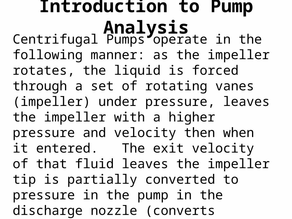
Introduction to Pump AnalysisCentrifugal Pumps operate in the following manner: as the impeller rotates, the liquid is forced through a set of rotating vanes (impeller) under pressure, leaves the impeller with a higher pressure and velocity then when it entered. The exit velocity of that fluid leaves the impeller tip is partially converted to pressure in the pump in the discharge nozzle (converts velocity head to pressure head). Flow is uniform, pump operates at a fixed sped (rpm).


Centrifugal Pump Characteristics:

Two pump parts:

1) rotating bowl called an impeller; forces the fluid being pumped into a rotary motion.

2) pump casing; designed to direct the fluid to the impeller and lead it away.


Sizing Centrifugal Pumps:

1) pump speed

2) impeller diameter


Centrifugal pumps - most commonly used in wastewater engineering

Radial-flow & Mixed-flow: pumps are used to pump wastewater and storm water.

Axial-flow: pumping treatment-plant effluent or storm drainage unmixed with wastewater.


Centrifugal pumps are classified to a type number known as the specific speed which varies with the shape of the impeller.

Specific Speed (Ns): The specific speed of an impeller may be defined as the speed in revolutions per minute at which a geometrically similar impeller would run if it were of such size as to deliver one gallon per minute against one foot of head.


Axial Flow Mixed Flow Radial FlowUsual capacity

rangeAbove 10,000 gpm Above 5,000 gpm Any

Head Range 0 to 40 ft 25 to 100 ft AnyHorsepower

characteristicsDecreases with

capacityFlat Increases with

capacity

Suction LiftUsually requires

submergenceUsually requires

submergence(lift limited)

Usually not over 15 ft

Specific Speed(English Units)

8,000 to 16,000 4,200 to 9,000Below 4,200 –single suctionBelow 6,000 –double suction

Service

Used where spaceand cost are

considerations andload factor is slow

Used where load factoris high and for servicewhere trash and other

solid material areencountered

Used where loadfactor is high and

high efficiency andease of maintenance

are desired

Pump Operating Range

A pump operates best at its bep because radial loads on the impeller bearings are at a minimum. Increasing the pump discharge beyond the bep the absolute pressure required to prevent cavitation

increases in addition to radial load problems. Decreasing the pump discharge toward the shut-off head (head at zero flow), recirculation of the pumped fluid causes vibration and hydraulic losses in the pump which may lead to cavitation.

Optimum operating range is 60 - 120 percent of the

bep

Characteristic Relationships For Centrifugal Pumps

Relationships were developed to predict the performance of centrifugal pumps at rotational speeds other than those for which the pump characteristic curves were developed.

Flow, head, and power coefficients

In centrifugal pumps, similar flow patterns exist in a series of geometrically similar pumps.

Applying dimensional analysis yields the following three dimensionless groups which can be used to describe the operation of rotodynamic machines including centrifugal pumps.


CQ= flow coefficient CH = head coefficient CP = power coefficient

Q = capacity H = head P = power input

N = speed, rpm = density

D = impeller diameter

3QCND

Q

22HCDN

H (8-7) (8-8)

53PCDN

P

(8-9)


Operating points at which similar flow patterns occur are called corresponding points. Eqs. 8-7, 8-8, 8-9 apply only to corresponding points.

Every point on a pump head-capacity curve corresponds to a point on the head-capacity curve of a geometrically similar pump operating at the same speed or a different speed.

Affinity LawsFor the same pump operating at a different speed, the diameter does not change and the following relationships can be derived from Eqs. 8-7 through 8-9.

2

1

2

1

N

N

Q

Q

22

21

2

1

N

N

H

H

32

31

2

1

N

N

P

P

(8-10) (8-11)

(8-12)

Eqs. 8-10 through 8-12 can be used to determine the effect of changes in pump speed on capacity, head and power of a pump.

Affinity Laws

The effect of changes in speed on the pump characteristic curves is obtained by plotting new curves using the affinity laws. This is illustrated in the following example.

Example 8-2. Determination of pump operating points at different speeds

A pump has the characteristics listed in the following table when operated at 1170 rpm. Develop head-capacity curves for a pump operated at 870 and 705 rpm, and determine the points on the new curves corresponding to Q = 0.44 m3/s (10.0 Mgal/d) on the original curve.

Cont. - Example 8-2.Pump Characteristics

Capacity,m3/s

Headm

Efficiency,%

0.0 40.0 ---0.1 39.0 76.50.2 36.6 83.00.3 34.4 85.00.4 30.5 82.60.5 23.0 74.4

Cont. - Example 8-2.

Solution:

1. Plot the head-capacity curves when the pump is operating at 1170, 870, and 705 rpm.

A) The plotting values for the reduced speeds are determined with the affinity laws (Eqs. 8-10, 8-11) as shown:

1

212 N

NQQ

2

1

212

N

NHH


b. The corresponding values are listed in the following table and plotted in Figure 8-19:

1170 rev/min 870 rev/min 705 rev/minCapacitym3/sec

Head,m

Capacitym3/sec

Head,m

Capacitym3/sec

Head,m

0.0 40.0 0.000 22.1 0.000 14.50.1 39.0 0.074 21.6 0.060 14.20.2 36.6 0.149 20.2 0.121 13.30.3 34.4 0.223 19.0 0.181 12.50.4 30.5 0.297 16.9 0.241 11.10.5 23.0 0.372 12.7 0.301 8.4


2. Determine the capacity and head at the other two speeds corresponding to Q = 0.44 m3/s on the original curve.

a) When the discharge is 0.44 m3s and the pump is operating at 1170 rev/min, the head is 28 m.

b) The corresponding head and capacity at 870 and 705 rev/min can be found using the following procedure:


i. First eliminate N1 and N2 from Eqs. 8-10 and 8-11 to obtain a parabola passing through the origin. 2

2 22

1 1

H Q

H Q=

2 212 2 22

1

HH Q kQ

Q= =


ii. Second, find the constant k for the curve passing through the points Q = 0.44 m3/s and H = 28.0 m. This can be determined using the following expression:

5

26.144/44.0

0.2823 m

s

sm

mk


iii. Third, determine the two other points on the parabola by using the above k value and plot the data in Figure 8-19.

mHQ

mHQ

mHQ

sm

sm

sm

8.520.0

0.1330.0

0.2844.0

3

3

3

Cont. - Example 8-2.iv. Finally, the corresponding points on the reduced-speed head-capacity curves are found at the intersections of the two curves and the parabola through the origin. The corresponding values are as follows:

mHQ

mHQ

sm

sm

1.10268.0

rev/min,705At

8.1533.0

rev/min,870At

3

3


Comment: The points in 2b(iii) have the same efficiency and specific speed as the corresponding point on the original curve.

Pump Specific SpeedFor a series of pumps with similar geometry operating under the same conditions, Eqs. 8-7 and 8-8 can be modified to obtain the following relationship which defines the pump specific speed.

4

3

21

43

31

21

21

22

3

/

/

H

NQ

DNH

NDQ

C

CN

H

QS (8-13)

Where,

NS = specific speed, dimensionless

N = speed, rev/min

Q = capacity, m3/s (gal/min)

H = head, m (ft)

Pump Specific SpeedSpecific Speed, NS :

For any pump operating at a given speed, Q and H are taken at the point of maximum efficiency.

Specific speed:

NS has no usable physical meaning, but is valuable because it is constant for all similar pumps and does not change with speed for the same pump.

NS is independent of both physical size and speed, but is dependent upon shape and is sometimes considered a shape factor.

Pump Specific SpeedPump design characteristics, cavitation parameters, and abnormal operation under transient conditions can be correlated to specific speed.

Further consideration of the specific-speed equation reveals the following:

1. If larger units of the same type are selected for about the same head, the operating speed must be reduced.

2. If units of higher specific speed are selected for the same head and capacity, they will operate at a higher speed; hence the complete unit, including the driver, should be less expensive. (e.g. it is obvious why large propeller pumps are used in irrigation practice where low-lift high-capacity service is needed.)

Example 8-3. Application of the specific speed relationship.

A flow of 0.20 m3/s (3200 gal/min) must be pumped against a total head of 16 m (52 ft). What type of pump should be selected and what speed should the pump operate for the best efficiency?

Cont.- Example 8-3

Solution:

1. Select the type of pump. Referring to Fig 8-7, the best efficiency for a pump at a flow of 0.20 m3/s is obtained by a pump with a specific speed of about 40 (interpolate between 0.190 and 0.63 m3/s curves).

The expected best efficiency is about 87 % and a Francis or mixed-flow impeller should be used.

Cont.- Example 8-3

2. Determine the pump operating speed.

a. Use Eq. 8-13 and substitute the known quantities to find the operating speed:

( ) ( )( )

13 21

2

3 34 4

ms

S

S

N rev/min 0.2NQN 40

H 16.0 m

N 40 0.0559N rev/min

40N 716 rev/min

0.0559

= = =

= =

= =

To meet the about conditions, the pump should operate at 716 rev/min. This speed would be possible if the pump were driven by a variable-speed drive.

Cont.- Example 8-3

2b. From a practical standpoint, if the unit is to be driven by an electric motor, the speed selected should be 705 rev/min for an induction motor (see Table 8-2) and the actual specific speed would be:

( ) ( )( )

13 21

2

3 34 4

ms

S

705 rev/min 0.2NQN 39.4

H 16.0 m= = =

Pump design presentation

Documents

Transcript of Pump design presentation