Published by Megger August 2015 ELECTRICAL TESTER · ELECTRICAL TESTER ... Published by Megger...

1 www.megger.com ELECTRICAL TESTER - August 2015

The industry’s recognised information tool

ELECTRICALTESTER

Published by Megger August 2015

The power of multifunctionPage 5

UNDERGROUND CABLES: preventing failure with partial discharge testing

Partial discharge (PD) measurements are

increasingly used as a reliable and non-

destructive diagnostic method for detecting

weak spots in the insulation of underground

cables. Partial discharge measurements are

also routinely used in laboratories for testing

cable reels prior to commissioning and in the

field to verify installation quality.

Typically, many factory-testing standards require

the use of 50/60 Hz high-voltage power supply

when performing laboratory tests. However,

the use of 50/60 Hz supplies has proven to be

impractical when it comes to field-testing, due

to high energy generation requirements.

The most important factor to consider when

choosing an alternative test frequency is that

the partial discharge characteristics at the

new frequency must be similar to those at

50/60 Hz, otherwise the results cannot be

reliably interpreted. This is especially true when

measuring partial discharge inception voltage

(PDIV), the voltage at which partial discharge

first occurs.

Partial discharge inception voltage is one of the

most important parameters used to characterise

partial discharge. If the PDIV measurement at

the new frequency is higher than at 50/60 Hz,

it may create false negatives, making problems

appear non-critical when they could in fact be

critical at the operating voltage.

Many research papers have addressed

the comparability of partial discharge

characteristics at various test frequencies and

with various wave shapes. This article provides

a quick overview of the most commonly used

test wave shapes.

0.1 Hz sinusoidal

The very low frequency (VLF) sinusoidal wave

shape was introduced for partial discharge

testing in the 1990s. In a scholarly paper, “Applied Voltage Frequency Dependence of Partial Discharges in Electrical Trees”,

researchers reported that PD is frequency

dependent and diminishes at low frequencies.

It is, therefore, challenging to measure partial

discharge at low frequencies such as 0.1 Hz.

A Megger research paper entitled, “Influence of the Test Voltage Wave Shape on the PD Characteristics of Typical Defects in Medium-

Voltage Cable Accessories” showed a greater

than 300% difference when interfacial

discharge was measured at 50 Hz compared

to 0.1 Hz. Additionally, the authors of the

paper conducted extensive literature research

on previous publications comparing PDIV

measurements at 50 and 0.1 Hz. Seven papers

reported a difference between the two values

that ranged from 10 to 250 percent.

This huge discrepancy is due to the

characteristics of interfacial discharge. Most

interfacial discharges in cable systems occur at

the terminations and in splices, and are very

dependent on the voltage gradient. A change

in voltage gradient could make the discharge

500 times smaller at 0.1 Hz compared to 50

Hz, which is a critical factor to consider when

making measurements with a VLF sinusoidal

test voltage.

Damped alternating current

Over the past 10 years, the damped alternating

current (DAC) technique has been established

as a very effective method for partial discharge

testing. This method is one of the voltage

shapes listed for PD testing in IEEE 400.3: “Guide for Partial Discharge Testing of Shielded Power Cable Systems in a Field Environment”.

Electric utilities have collected numerous

examples of successful field test data that show

a very strong correlation between 50/60 Hz and

DAC results. This correlation prompted a broad

comparative study of commercially available

medium-voltage cable diagnostic systems by

Centro Elettrotecnico Sperimentale Italiano

Giacinto Motta (CESI), an Italian company

that provides testing and certification services,

energy consultancy, engineering and technology

consulting for the power sector globally.

Table 1 shows the different voltage shapes

compared in the study. Testing was performed

on five cables. Three parameters – the partial

Henning Oetjen - Product manager

VF / HDW cable products

SYSTEM SOURCEA Sinusoidal voltage at power frequency

B Sinusoidal voltage at very low frequency (0.1 Hz)

C Oscillating wave within power frequency and low damping (DAC)

D Oscillating wave with fixed frequency and high damping

Table 1: Test voltage wave shapes used in a study carried out by engineering company CESI

Continued on page 3

Power swing simplificationPage 6

I033_Electrical Tester_JUL15_V02.indd 1 23/06/2015 11:31

2 ELECTRICAL TESTER - August 2015 www.megger.com


ELECTRICALTESTER

Contents

Editor Jeremy Hewlett

T +44 (0)1304 502232

E [email protected]

Megger Limited

Archcliffe Road Dover Kent CT17 9EN

T +44 (0)1304 502100

E [email protected]

www.megger.com

‘Views expressed in Electrical Tester are not necessarily the views of Megger.’

The word ‘Megger’ is a registered trademark

A printed newsletter is not as interactive as its email equivalent

so to help you find items quickly on www.megger.com, we have

underlined key search words in blue.

The rights of the individuals attributed in Electrical Tester to be

identified as authors of their respective articles has been asserted

by them in accordance with the Copyright, Designs and Patents

Act 1988. © Copyright Megger. All rights reserved. No part

of Electrical Tester may be reproduced in a retrieval system, or

transmitted in any form or by any means, electronic, mechanical,

photo-copying, recording or otherwise without the prior written

permission of Megger.

To request a licence to use an article in Electrical Tester, please

email [email protected], with a brief outline of the

reasons for your request.

All trademarks used herein are the property of their respective

owners. The use of any trademark in this text does not imply

trademark ownership rights in such trademarks, nor does use

of such trademarks imply any affiliation with or endorsement of

Electrical Tester by such owners.

When you have finished with this magazine please recycle it.

discharge inception voltages, the location

of partial discharge spots and the PD pulse

amplitudes – were selected as the comparison

criteria. Figure 1 shows an excerpt from

the results. Overall, the damped alternating

current method proved very similar and the

most comparable to 50-Hz testing while 0.1

Hz sinusoidal showed the largest deviation.

0.1 Hz cosine rectangular

The first very low frequency systems used a

cosine rectangular (CR) wave, which proved

very effective, and is still widely used because

the time interval of its polarity change

replicates that of a 50/60 Hz wave. Figure 2

shows the characteristic shape of the 0.1 Hz

CR wave compared to the damped alternating

current and the 0.1 Hz sine wave.

In 2003, German author and scientist Daniel

Pepper performed in-depth research to evaluate

merits of using a triangle voltage shape and a

very low frequency cosine rectangular voltage

shape as voltage sources for partial discharge

testing on solid dielectric power cables. Both

wave shapes performed well for this purpose;

however, the cosine rectangular showed

higher partial discharge levels, especially for

sliding discharges.

Test wave generation

VLF Cosine Rectangular Voltage

The VLF cosine rectangular voltage is

generated by a circuit as shown in Figure 3.

One of the most significant advantages of the

CR technology is its ability to store and recover

90 percent of the energy within the charged

cable via the choke. The stored energy is used

to charge the cable with the opposite polarity

during the next half cycle, within the same

millisecond interval of the 50/60 Hz operating

frequency. This allows substantially higher test

loads to be driven with fairly small input power

compared to sinusoidal VLF systems. VLF

cosine rectangular systems with up to 25 μF

and 20 to 80 kVrms are commercially available.

Damped AC Voltage

The circuit used for generating a DAC

voltage is fundamentally similar to the one

used for generating a VLF cosine rectangular

voltage. The only difference is how switch

“S” operates. In the VLF cosine rectangular

system, the switch reverses its position to allow

polarity reversal. In the DAC system, this switch

closes after allowing the cable to be charged to

the test voltage, creating a damped resonance

(fixed) circuit. The resonant frequency of

the circuit is a function of the inductance of

the choke, the capacitance of the auxiliary

capacitor and the capacitance of the cable to

be tested.

Advantages

The two main advantages of very low frequency

cosine rectangular technology are its energy

efficiency due to its resonant design, and the

polarity reversal time interval on the VLF cosine

rectangular very closely matching the one at

50/60 Hz, so that it mimics the electrical stress

on the insulation under operating conditions.

This close time matching makes the technology

an excellent candidate for use as a power

supply in offline partial discharge testing.

The same two characteristics make VLF cosine

rectangular technology a very effective tool

for withstand testing (with or without partial

discharge monitoring), enabling the testing

of very long cables or simultaneous testing of

three phases at 0.1 Hz. In contrast, damped

alternating current technology is not ideal

for withstand testing because it requires a

substantial number of test cycles to generate

an equivalent amount of electrical stress for

the same duration. This shorter exposure time

to the electrical stress at power frequency is

exactly what makes DAC perfect for truly non-

destructive partial discharge diagnosis.

Applications

Given the advantages of the VLF cosine

rectangular wave shape, its performance as

a voltage source for offline partial discharge

testing was evaluated. In this study, partial

discharge inception voltage and partial

discharge levels were measured at the

operating voltage (U0) on service-aged cross-

linked polyethylene (XLPE) and paper-insulated

lead covered (PILC) mixed cables using both

VLF cosine rectangular and DAC methods.

The damped alternating current method

was chosen for comparison instead of 50/60

Hz because DAC results have already been

established by numerous studies as being

highly correlated with 50/60 Hz results. Table

2 summarizes the test parameters for each of

the three tests.

Figure 4 shows the on-site test set up for

partial discharge measurements. As discussed

previously, both the DAC and VLF cosine

rectangular test voltages can be generated

with the same circuit by controlling switching

behaviour. The measurements were performed

with conventional coupling and without any

hardware or software noise filtering.

In summary, both methods produced very

similar partial discharge inception voltage

(PDIV) and maximum partial discharge

(PDmax) values (refer to Tables 3, 4, and 5)

with acceptable statistical fluctuations. Both

methods were able to identify the same weak

spots in all three cables.

PARAMETER TEST 1 TEST 2 TEST 3

Cable insulation type XLPE PILC / XLPE PILC / XLPE

System voltage 22 kV RMS 11 kV RMS 11 kV RMS

Cable length 1,563 ft

(469 m )

2,206 ft

(662 m )

5,430 ft

(1,629 m)

Installation year 1985 1960 1965 / 2004

Cable age at time of test 26 years 51 years 46 years

Figure 2: Comparison of DAC, 0.1 Hz sine wave and 0.1 Hz CR wave shapes. The time taken for the polarity reversal with the VLF CR wave shape closely matches that of the DAC but its peak voltage is maintained for five seconds until the next cycle in the VLF CR system.

Table 2: Summary of test parameters

Continued from page 1

UNDERGROUND CABLES: preventing failure with partial discharge testingr .......................................................Page 1-3 Henning Oetjen - Product manager VF / HDW cable products

Development and field experience of Turns Ratio Testing ..........................................p3

Jialu Cheng - Application engineer

Multifunction comes to power. ............. P5Peter Fagerstrom - Business unit manager

Diagnostic testing of high voltage circuit breakers – Part 2 .........................Page 4 -5Roberts Neimanis - Application specialist

Testing power swing and out-of-step relay elements using simplified equations ..........................................................Page 6 Jason Buneo - Applications development manager

Q and A ...................................................p8

One stop protection condition analysis ............................................Page 8 Stefan Larsson - Power product manager

Missed an edition?

You can find every edition of Electrical Tester since 2007 on our website - visit www.megger.com

Figure 1: Comparison of PDIV at 50 Hz with each test system. Overall, the DAC method (green) was most closely comparable with 50/60 Hz testing and the 0.1 Hz sinusoidal (red) showed the largest deviation.




ELECTRICALTESTER

PDmax values were generally slightly higher

with VLF cosine rectangular. The VLF cosine

rectangular waveform consists of a millisecond

polarity reversal, followed by a five-second

plateau of the peak voltage before the next

cycle. This plateau phase most likely causes

an accumulation of charges at the layered

interfaces of the cable, resulting in higher PDmax

values. Furthermore, this phenomenon might

explain why the VLF cosine rectangular allows

weak spots on longer cables to be located

more easily.

Last words

Partial discharge measurements using

VLF cosine rectangular test waves were

benchmarked against the well-established

damped alternating current method. The results

showed that PDIV, PDmax, and the location

of weak spots obtained by the VLF cosine

rectangular method were highly comparable

to the DAC method. This proves that the VLF

cosine rectangular wave shape is a comparable

and convenient voltage source for partial

discharge testing in the field. The similarity in

the design of the VLF cosine rectangular and

DAC voltage generation circuit means that it

is possible for VLF cosine rectangular units to

also generate a DAC voltage. The integration

of both technologies offers users the flexibility

of a single unit that can perform withstand

testing, partial discharge monitored withstand

testing, and non-destructive PD diagnostics

with damped alternating current.

Figure 3: Block diagram of a VLF CR unit

Figure 4: Set up for partial discharge test

TEST PHASE L1 L2 L3

1XLPE Cable 1,563 ft (469 m)

Test voltage DAC VLF CR DAC VLF CR DAC VLF CR

PDIV ( kV RMS) 13.2 12.0 10.8 14.0 12.0 12.0

PDMAX (pC) @ U0 300 620 310 - 125 490

Table 3: Comparison of PDIV and PDmax for DAC and VLF CR (Test 1)

TEST PHASE L1 L2 L3

2Mixed Cable 2,206 ft (662 m)


PDIV ( kV RMS) 4.2 6.0 4.2 3.0 4.2 3.0

PDMAX (pC) @ U0 2,350 1,100 600 1,400 2,650 9,300


TEST PHASE L1 L2 L3

3Mixed Cable 5,430 ft (1,629 m)


PDIV ( kV RMS) 42.4 6.0 2.4 <3.0 2.4 <3.0

PDMAX (pC) @ U0 9,500 7,400 6,545 5,500 14,980 50,000


The transformer turns ratio (TTR) test is very important; it confirms that the transformer has the correct ratio of primary turns to secondary turns. Using this test correctly can help to identify shorted turns, open windings, incorrect winding connections and other faults inside transformers.

The principle of TTR is that an AC voltage V1 is applied to the primary side of the transformer and the induced voltage V2 at the secondary side is measured. For single phase transformers, the transformer voltage ratio, TVR, is equal to the transformer turns ratio, TTR: where, N1 is the primary winding number of turns and N2 is the secondary winding number of turns. The transformer nameplate ratio, TNR is determined by TTR and the vector group. The tester measures the voltage ratio TVR and then calculates TNR and TTR based on the winding connections. Therefore, information about the correct vector group should be available when performing the turns ratio testing.

N1

N2

V1

V2

=

However, tests in special applications, such as those involving phase shift transformers, can be difficult with single-phase instruments. These transformers usually have a phase shift of 30° ± 7.5°. A new algorithm introduced in IEC 61378-1 Ed.2 proposes a solution to test phase-shift transformers with single-phase instruments. The test parameters and calculation methods

are based on a geometrical and trigonometrical approach. Instruments in the latest Megger TTR series apply the algorithm. They are also able to detect the vector group of the tested object so the nameplate information is not necessity any more.

IEEE standard (C57.152) states that when the rated voltage is applied to one winding of a transformer, all other rated voltages at no load shall be correct within 0.5% of the nameplate readings. The deviation is calculated by:

Deviation%= Measured ratio − Nameplate ratio

x 100% Nameplate ratio

Field experience has shown that shorted turn-to-turn fault might be difficult to identify if only referring to the ratio results. Figure 1 is the TTR test result for a transformer that tripped because of a turn-to-turn short circuit. The results look very good and no problem can be found. But the excitation current provided more information about the fault.

The best TTR testers have the ability to measure the excitation current during turns ratio testing. In this case, the excitation current of phase A reaches 257 mA when the test voltage goes to 100 V! This is the strong evidence indicating that there is something wrong with the transformer.

It is also worth noting that results from hand held TTR testers sometimes show deviations larger than expected for instrument transformers. It is recommended to use testers with relatively higher test voltage such as 80 V for those high-ratio transformers. Because higher voltage improves the core excitation level as well as the measurement accuracy.

Development and field experience of Turns Ratio Testing

Figure 1. Turns ratio testing results from a transformer with 19 primary taps

Jialu Cheng - Application engineer




ELECTRICALTESTER

Introduction

This is the second part of our article dealing with the important subject of circuit breaker testing. The first part, which covered standards, circuit breaker types and some of the most commonly performed tests, appeared in the last issue of Electrical Tester, which is still available on line. This second part covers more test techniques and, in particular, looks at the relatively new approach of resonant frequency testing.

Coil test

If the current in the operating coil of a circuit breaker is monitored during a trip operation, a curve similar to that shown in Figure 1 will be obtained. When the trip coil is first energized [1], current flows through its windings. The magnetic lines of force in the coil magnetize the iron core of the armature, in effect inducing a force in the armature. The current flowing through the trip coil increases to the point where the force exerted on the armature is sufficient to overcome the gravitational and frictional forces that tend to keep the armature at rest. When this point is reached, the armature is pulled [2] through the trip coil core.

The magnitude of the initial current [1-2] is proportional to the energy required to move the armature from its initial rest position. The movement of the iron core through the trip coil generates an electromagnetic force in the coil that in turn has an effect on the current flowing through it. The rate of rise of current depends on the change in the inductance of the coil.

The armature operates the trip latch [3-4], which in turn releases the trip mechanism [4-5]. The anomaly at [4] is the point where the armature momentarily stops as contact is made with the prop. More energy is required for the armature to resume motion and overcome the additional loading of the prop. The anomaly may be caused by degradation of the prop bearings, lubrication, changes in temperature, excessive opening spring force or mechanism adjustment. The armature completes its travel [4-5] and hits a stop [5].

Of particular interest is the section of the curve between [4] and [5]. As the armature moves from the point where the trip mechanism is unlatched [4] to the stop [5] the inductance of the coil changes. The curve is an indication of the speed of the armature. The steeper the curve the faster the armature is moving. After the armature has completed its travel and has hit the stop [5], there is a change in current signature. The magnitude of the current [7] is dependent on the DC resistance of the coil. The ‘a’ contact opens at [8] to de-energize the trip coil and the current decays to zero.

The interpretation of the circuit breaker operating coil signature often provides useful information about the condition of the latching systems.

Minimum voltage test

This test is often neglected even though it is specified and recommended in international standards. The test objective is to make sure that the breaker can operate at the lowest voltage level provided by the station battery during a power outage. The test is performed by applying the lowest specified operating voltage and verifying that the breaker operates within specified parameters. The standard test voltages are 85% and 70% of nominal voltage for close and open operations respectively.

Minimum voltage required to operate the breaker

This test, which should not be confused with the minimum voltage test just described, determines the minimum voltage at which the breaker is able to operate. It is a measure of how much force is needed to move the coil armature. This test is not concerned with contact timing parameters, only whether the breaker operates or not. The test starts by sending a control pulse at a low voltage to the breaker. If the breaker doesn’t operate, the voltage is increased by, say, 5 V and the test is repeated. This procedure is continued, with gradually increasing voltage, until the breaker

eventually operates. The voltage at which this occurs is recorded and, if the test is repeated next time the breaker is maintained, a comparison between the old and new figures will indicate whether significant changes have occurred.

Vibration testing

Vibration testing is based on the premise that all mechanical motion in equipment produces vibrations, and that by measuring them and comparing the result with the results of previous tests (known data), the condition of the equipment in question can be evaluated.

The easiest parameter to measure is the total vibration level. If it exceeds a specified value, the equipment is deemed to be in the fault or at-risk zone. For all types of vibration testing, a reference level must have been previously measured on equipment known to be fault free. All measurements on the equipment tested are then related to this reference signature in order to determine whether the measured vibration level is “normal” or whether it indicates the presence of faults.

Vibration analysis is a non-invasive test technique that uses an acceleration sensor with no moving parts. The breaker can stay in service during the test; an open-close operation is all that is required for the measurement. First-trip operation can be different from the second and third because of corrosion and other metal-to-metal contact issues. Vibration is an excellent method to capture the data about the first operation after the breaker has spent a long time in the same position.

The analysis of vibration data involves comparing the latest results with the reference. Vibration measurement can detect faults that are barely noticeable using other conventional methods. However, if data such as contact timing, travel curve, coil current and voltage are available in addition to the vibration data, even more precise condition assessment is possible.

Vacuum bottle test

Vacuum bottles in vacuum circuit breakers are tested with high voltage AC or DC to confirm the integrity of the vacuum. The electrical behaviour of the vacuum in the bottle is identical for AC and DC. The main difference in using DC and AC is that AC measurements are influenced by capacitance. The resistive current component is typically between 100 and 1,000 times smaller than the capacitive current component, and the resistive component is therefore difficult to distinguish when testing with AC. As a result, AC requires much heavier equipment for testing compared to DC test instruments.

Both the DC and the AC methods are detailed in standards ANSI/IEEE 37.20.2-1987, IEC 694 or ANSI C37.06.

Synchronized switching

In order to test the function of a controlled switching device one or more currents from current transformers and reference voltages from voltage transformers are recorded, along with controller output signals, while issuing an open or close command. Details of the test set up depend on the test instrumentation, as well as the available voltage and current sources.

SF6 leakage

SF6 leakage is one of the most common problems with circuit breakers. The leakage can occur in any part of the breaker where two components are joined, such as valve fittings, bushings and flanges. In rare cases, SF6 can also leak straight through the aluminium as a result of poor casting.

Leaks can be found by using gas leak detectors (sniffers) or thermal imaging.

Humidity test

As humidity can cause corrosion and flashovers inside a breaker, it is important to verify that the moisture content inside an SF6 breaker is minimal. This is done by venting a small amount of SF6 gas from the breaker through a moisture analyser, which will determine the moisture content of the gas.

Air pressure test

Air pressure testing is carried out on air-blast breakers. Pressure level, pressure drop rate and airflow are measured during various operations. The blocking pressure that will block the operation of the breaker in the event of very low pressure may also be measured.

A new approach: resonant frequency testing

Preparation for testing a circuit breaker involves the safe isolation of previously energised high-voltage equipment. Ground connections are then applied to the isolated equipment, normally leaving breaker grounded on both sides. Present practice for performing timing tests requires, however, that the ground connections on one side of the breaker are removed during the test to allow correct operation of the test equipment.

The potential safety issues with this practice require the adoption of special safety procedures. In most cases, an “authorised person” will be involved with the test as well as a central office that issues the special work permits required. This means that the test takes longer, tying up equipment and the test engineer unnecessarily. In addition – and most important – the network is out of service for longer. Engineers also need more training so that they can deal with the necessarily complex safety procedures.

To address these issues, a new technology was introduced in 2006 that allows main contact timing tests to be performed on a circuit breaker with both sides grounded. Dangerous voltages can, therefore, be kept at distance – a safe area around the circuit breaker can be created and clearly marked with security fencing. Accidents with electric arc and electrocution can be avoided. The main contact timing results produced by this new technology are fully compatible with the conventional main contact timing measurement. For field personnel, the new way of working is much faster but is otherwise familiar.

This new timing technique is based on the capacitance formed between the parts of the breaker contact, which are separated by an insulating medium – usually oil, air, vacuum or SF6. Any circuit breaker contact can, therefore, be seen as a capacitor. This capacitor is a part of the resonant circuit formed by breaker itself and other surrounding components such as busbars, connections and ground connections, as shown in Figure 2.

The resonant frequency of the circuit depends on the value of the capacitance between circuit breaker contacts and the circuit response will vary with the movement of the contacts, as shown in Figure 3.

Timing of main contacts can be performed using this technique, which is also called the DualGround method. This is a revolutionary method that allows circuit breakers to be tested more safely and more efficiently than with conventional timing techniques. Safety dictates that both sides of a breaker should be grounded during field tests but conventional timing

Diagnostic testing of high voltage circuit breakers – Part 2

methods require ground to be disconnected on one side of the breaker to allow the instrument to sense the change in contact status. This procedure makes the test cables and the instrument part of the induced current path while the test is being performed.

The DualGround method allows for reliable measurements with both sides of the circuit breaker grounded thus making the test safer, faster and easier. This technique also makes it possible to test circuit breakers in configurations such as GIS applications, generator breakers and transformer applications where conventional timing methods requires removal of jumpers and busbar connections, which is difficult and inconvenient.

Comparison with other methods

DualGround timing is an excellent solution when ground loop resistance is low since it has no lower limit for ground loop resistance. The ground loop can even have lower resistance than the main contact/arcing contact path without affecting the results. This is particularly crucial when testing GIS breakers and generator breakers, as well as for AIS breakers having good grounding appliances. The changes in resonant frequency of the whole circuit (breaker and ground loop) can easily be used for close/open status detection.

Often dynamic resistance measurement is proposed as a tool for timing circuit breakers with both sides grounded. In this case, the determination of circuit breaker state is made by evaluating the resistance graph against an adjustable threshold. If the resistance is below the given threshold the circuit breaker is considered closed while if the resistance is above the threshold the circuit breaker is considered open.

Problems can arise, however, when choosing the threshold since it must be below the ground loop resistance (which is initially unknown) and above the resulting resistance of the arcing contact (which also is unknown) and the ground loop in parallel. The reason is that, according to the IEC standard, it is the closing/opening of the arcing contact that is considered as the operation time of the circuit breaker, not the main contact, and the difference between main and arcing contact operation time can, depending of contact speed, be as much as 10 ms. For example, a 2 x 10 m copper grounding cable with 95 mm2 cross section area has a resistance of about 3.6 mΩ (not counting the resistance of connector devices). An arcing contact is usually also in the mΩ range, from a couple of mΩ up to about 10 mΩ, depending on the type of circuit breaker and on the condition of the arcing contact. All this taken together makes it a near impossible task to adjust the threshold, as the exact value to use is unknown. It may require several attempts to achieve a reasonable result and may be even more difficult if the resistance graph is not recorded during measurement.

Furthermore, a method that relies on evaluation against thresholds is more sensitive to induced AC currents through the test object. When a circuit breaker is grounded on both sides a loop is formed with a large area exposed to magnetic

Roberts Neimanis - Application specialist

Figure 1 – Detail of coil current signatureFigure 3 – Change of voltage in resonance circuit

Figure 2 – Resonant frequency model of circuit breaker grounded on both sides.




ELECTRICALTESTER

Diagnostic testing of high voltage circuit breakers – Part 2

fields from surrounding live conductors. The alternating magnetic field will induce a current in the circuit breaker/grounding loop. This current can reach a few tens of amps, which corresponds to a significant proportion of a typical 100 A test current. If the evaluation threshold is at the limit, these induced currents will definitely affect the timing results. The resonant frequency technique is, on the other hand, completely insensitive to 50/60 Hz interference.

Conclusions

Breakers are complicated, mechanically sophisticated devices that require periodic adjustment. Sometimes a technician can see the need for these adjustments with a visual inspection, and the problem can be solved

without testing. However, with most circuit breaker issues, testing will be required. When maintaining a circuit breaker, technicians should start with timing and motion measurements. In fact, if that technician only has time for a single measurement, that measurement should be timing.

Electrical power network growth and asset development requires that all available technologies be implemented to ensure reliable electricity supply. New technology for circuit breaker testing offers a more cost efficient test procedure and, since it allows both sides of the breaker to be grounded during testing, it ensures safety for key employees in accordance to national laws, standards and social partners demands.

Figure 4 – Connections to breaker using conventional and DualGround technique

Figure 5 – Potential for error when using dynamic resistance measurement for timing a circuit breaker with both sides grounded.

It is still common practice in substation testing to use separate instruments for each type of test. This situation, however, is about to change. There are many compelling reasons to move away from separate instruments in favour of a multi-functional test set, including:

1. Users always have all of the test facilities they need readily at hand; no need to go back to the van or, worse, back to base to fetch another instrument for the next test. Plus, a single multifunction tester is much easier to transport than several individual instruments.

2. Multi-functional test sets cost less than the individual instruments that would be needed to cover the same range of testing requirements; e.g., four single-function test instruments = four displays, four user interface systems, four enclosures, etc. = more $¥€ than one multifunction instrument with one display, one UI system, one enclosure, etc.

3. Reduces testing time so saves money; only one instrument to unpack, power up and configure; the same cable set is used for a whole range of measurements, so the connections only need to be made once; and, when carrying out a range of tests, users of multifunction instruments move quickly and easily from app to app, rather than having to go from instrument to instrument.

4. Less operator training is required; users of separate instruments need to familiarise themselves with the quirks of each, whereas users of well-designed multifunction testers enjoy a consistent user interface across all functions, which means that the learning process is simplified.

This begs the question then, if multifunction instruments have so much to offer, why are they not used more frequently for substation testing? The reasons are interesting:

1. Inertia. If separate instruments have always been used in the past and have delivered satisfactory results, why change? The simple answer is that change brings the benefits above.

2. Cost. If an additional single-function instrument is all that’s needed to complement instruments already owned, why spend extra on a multifunction tester that will duplicate at least some of the functionality of the existing instruments? The answer is an investment for the future. Buy a multifunction tester and it will probably be unnecessary to replace the single-function instruments as they come to the end of their lives.

3. Until recently, few, if any, adequately specified instruments were available. This is not particularly surprising, as designing and manufacturing a versatile, convenient, dependable and easy-to-use multifunction tester for use in substations presents many challenges.

A multifunction test instrument design that can lead a migration from single-function instruments must:

n be capable of generating high currents and voltages yet remain easy to transport. For users with interests that cover a wide geographical area, it is highly desirable for the instrument to weigh less than the international maximum shipping weight of 32 kg for check-in luggage on passenger flights.

n alleviate the potential conflict between versatility and ease of use. There’s little point in producing a multifunction instrument that can perform a wide range of tests if many of the tests are difficult to access and set up. This only leads to user frustration and ultimately dissatisfaction with the product, however impressive its claimed abilities may be.

Fortunately, recent advances in instrument design and technology have made it possible to produce multifunction testers for substation and other power applications that address both of these issues, making them truly attractive to users. An excellent example is a recently released integrated transformer and substation test system.

This compact unit, the main section of which weighs just 26 kg, provides comprehensive facilities for testing power transformers, current transformers, potential transformers, circuit breakers, rotating machines and many other items of substation equipment. The base unit can generate AC current up to 800 A, DC current up to 100 A, AC voltage up to 2.2 kV and DC voltage up to 300 V. With optional accessories, the AC capabilities can readily be extended to 2,000 A and 12 kV.

The voltages and currents generated by the instrument can be controlled and measured with a high degree of precision, allowing it to be used for an exceptionally wide range of applications that includes, for example, turns ratio, winding resistance and excitation current measurements in transformers; contact resistance, impedance and tan delta/power factor testing; main and resistor contact timing in circuit breakers; and primary injection testing in LV, MV and HV equipment of almost any type.

The challenge of delivering a simple user interface and experience in view of this vast range of capabilities has been met by making use of the latest colour touch-screen technology and by designing the user interface so that it presents functions in the form of apps (“virtual instruments”). When the user has decided what to measure and has selected the app/instrument to work with from the start screen, the display shows only those elements that are appropriate to that function.

For example, if the winding resistance instrument is selected, the screen simply shows the output current, the output voltage and the measured resistance. The user selects a test current and starts measuring. Users, who prefer test guidance from the instrument, just enter the configuration and the unit provides connection diagrams and a table showing the sequence of measurements.

Provision is also made for full manual testing with a generic instrument app that allows the user to freely select outputs, measurement inputs and the way in which the measured data should be processed.

This remarkable new multifunction substation test set – the Megger TRAX – conveniently and cost effectively replaces a whole battery of conventional single-function instruments. Let the migration begin.

Peter Fagerstrom - Business unit manager

Multifunction comes to power




ELECTRICALTESTER

The method

Past methods of testing power swing and out-of-step conditions have often involved a brute force approach of applying voltages and currents to simulate impedances seen by the relay. By manually ramping the impedance trajectory, or playing several vector states where specific impedance was applied, it was possible to trick the relay into seeing an impedance tracking across the measurement zones. However, trying to trick new relays with more advanced algorithms doesn’t work. The relay is looking for a smooth transition between the measurement zones, and if it does not see it, then it will not block the power swing or trip on the out-of-step.

To satisfy the conditions for the power swing and out-of-step algorithms currently in use, a new method is proposed. By superimposing two waveforms of similar frequencies, a smooth impedance ramp can be achieved. This method is similar to a two-source model in that both sources have similar frequencies and amplitudes. The rate of change of impedance can be controlled as well as the minimum and maximum impedances, the number of pole slips, and the starting phase angle relationships. The characteristic equation of the output waveform for the voltage and current is as follows:

Eq. 1 f(I,V)

(t) = (A1sin(ω

1t + ϕ

1))

+A2 sin(ω

2t +ϕ

2 )

Where:

A1 = Magnitude of current/voltage source 1 as an RMS value

ω1 = 2π*FrequencySource1 , (Frequency is in Hz, ω1 is in rad/s)

ϕ1 = Initial phase angle of current/voltage source 1 in degrees

A2 = Magnitude of current/voltage source 2 as an RMS value

ω2 = 2π*FrequencySource2 , (Frequency is in Hz, ω2 is in rad/s)

ϕ2 = Initial phase angle of current/voltage source 2 in degrees

t = the time of the event in seconds

Using arbitrary values for Equation 1, Figure 1 shows the plot of a voltage and current waveform with the following parameters:

V1= 49.5 V, V2=19.5 V, I1=16.725 A,

I2=13.275 A, F1=60 Hz, F2 = 59 Hz, ϕ1Current

= 0°, ϕ2Current = 0°, ϕ1Voltage = 0°, ϕ2Voltage = 0°

Both the voltage and current waveforms decrease and increase at the same time and

remain in phase for the duration of the waveform plot. This is not the behaviour of a power swing or out-of-step condition. To change this, the phase current needs to be offset by 180°. The

option is to change either ϕ1Current or ϕ2Current. By

changing ϕ1Current, the phase angle will initially start 180° out of phase and then slowly come back into phase, then go back out, and repeat indefinitely. Since it is desirable to control the

phase angle from the start, ϕ2Current will be set to 180°. This will allow the two waveforms to start in phase and then slowly go out of phase and come back into phase, and repeat. A plot of the waveforms with the appropriate phase shift is shown in Figure 2.

This is the general form of the power swing waveform. Next is a discussion on how to implement a controlled power swing and out-of-step condition using any of the Megger SMRT test systems.

Applying the method

Power Swing

To apply a power swing, the following parameters need to be defined.

1. The Maximum Impedance, Zmax, of the Power Swing/Out-of-Step needs to be defined. This will be based on the outermost characteristic that is tracking the impedance. It is recommended that the maximum impedance be greater than the largest blinder/characteristic impedance, but not so large that the trajectory of the swing exits the characteristic prematurely.

2. The Minimum Impedance, Zmin, of the Power Swing/Out-of-Step also needs to be defined. This will be the stopping point of the swing/step.

3. The Source Frequencies will determine the duration of a single power swing or out-of-step condition. The source frequencies will also affect the rate of change of the trajectory of the impedance. The larger the difference in frequency between the two sources, the faster the swing/step, and the smaller the difference, the slower the swing/step.

4. The Starting Phase Angle needs to be defined so that proper loading conditions can be simulated.

Here is how to create a power swing with a

maximum impedance of 15 Ω, a minimum

impedance of 1 Ω, a Source 1 Frequency of

60 Hz, a Source 2 Frequency of 59 Hz, and a starting Phase Angle of 0°.

The first parameter that we can determine is how long a complete power swing cycle will take, tSwing. This is given by Equation 2.

Eq. 2 tSwing

= 1

(f1- f2) (s)

Putting our values into this equation:

t

Swing= 1

(60-59)=1 s

When applying this method to any type of test routine, tSwing should be set for the maximum time the swing should be applied. If multiple turns are desired, then maximum time is the number of turns times tSwing.

Next, we will be solving for the currents and voltages that should be applied to the relay. To start, only the A phase voltage and current will be discussed. B and C phases are identical to A, with the appropriate phase shifts. A nominal voltage should be defined for the maximum impedance, and a fault voltage should be defined for the minimum impedance. Take care in choosing a fault voltage. Some of the impedances could still be quite large, with large being defined as around 15 Ω or greater. If the fault voltage is too small, negative currents will be calculated to create the correct conditions. If this happens, increase the fault voltage until the currents are at an acceptable level. For this example the nominal voltage, Vnom, is 69 V line-to-ground, and the fault voltage, Vfault, is around 30 V line-to-ground.

The value of Vfault can change depending on the impedance and the current required from the test system. The variable name Vfault can also be a little misleading. A power swing event may not necessarily involve the extreme values of traditional fault voltages. The impedance swing may only go from a large value to a slightly smaller value. This would be the case if the user wanted to swing from 89 Ω to 50 Ω. The required fault voltage would not be much less than that required for starting impedance.

The equations for the two voltages for phase A are:

Eq. 3 V1 = Vfault

+ (Vnom

− Vfault)

2

Putting our values into this equation:

V

1= 30 + (69 − 30) 2

= 49.5 V

Eq. 4 V2 = (Vnom

− Vfault)

2

Putting our values into this equation: V2= (69 − 30) 2

= 19.5 V

Then the two currents for I1 and I2 will be solved.

Eq. 5

I1=[(Vfault)

- ((Vfault)

- (Vnom)) Zmin

Zmin

2

Z

max ]

Using our values:

]]I

1=[(69)

– (( 30) – (69)) 1

1 15 = 17.3A

2 ]

Eq. 6

I

2=((V

fault)

- (Vnom))

Zmin

Zmax

2

Using our values:

I

2=((69)

- (69)) 12.7 A

1

15

2

Other parameters can now be solved such as the rate of change of impedance. Since the swing goes from maximum impedance to a minimum and back again, the rate should only be calculated based on the time it takes to go from the maximum to the minimum. This is shown in Equation 7.

Testing power swing and out-of-step relay elements using simplified equations

Figure 1: Superimposed voltage and current waveforms

Figure 2: Plot of voltage and current waveforms with current offset by 180°

Figure 3 – Waveform capture of a power swing

Jason Buneo - Applications development

manager




ELECTRICALTESTER

Eq. 7 Z

rate = 2 * (Z

max - Z

min) tswing

Using our values:

Zrate

= 2 * (

15 - 1) 1 = 28 W/s

When starting in the pre-fault mode for testing, it is handy to be at the same current level as the starting current for the swing. This is minimum current, which is given by Equation 8.

Eq. 8

Imin

=I1 - I

2

Using our values: I

min = 17.3 - 12.7 = 4.6 A

For practical applications, three states can be used to simulate a pre-fault, fault and post-fault state. Figure 3 shows recorded waveforms from the Megger SMRT relay test system.

The time set for the Pre-Fault duration is critical in that it is necessary for the waveform to end at the precise phase angle and magnitude that is equal to the start of the power swing event. The Pre-Fault phase angle of the current should be equal to the starting phase angle of the power swing. In Figure 3, the duration was set for 1 second, and the calculated time of 1 power swing was also 1 second. By setting the Pre-Fault to the same time as the calculated time of the power swing, a smooth transition is guaranteed in the waveforms. The time can also be set to an integer multiple of the swing duration. In this case, 2, 3, or 4 seconds would also work. A time of 0.5 seconds would not work. This is shown in Figure 4.

Comparing Figure 3 and Figure 4, the shift of the power swing characteristic is apparent when the Pre-Fault duration is changed to a value other than an integer multiple of the time of the swing event. The Pre-Fault duration, or any state before a swing event should be set according to Equation 9.

Eq. 9 Tprefault

= N * tSwing

Where N is an integer (whole number)

It should be noted that if it is desirable to have flexible Pre-Fault times, the initial current and voltage magnitudes can be solved for using Eq. 1 for the applied times.

Testing power swing and out-of-step relay elements using simplified equations

Figure 4 – Power Swing with Pre-Fault Duration changed to 0.5 s

Figure 5 – Phase angle of the power swing in degrees vs time in seconds

Figure 6 – Trajectory of impedance during a power swing

Figure 7 – Waveform capture of an out-of-step condition

While testing the power swing element, other parameters should be displayed as well. The user will be interested to see the impedance trajectory of the power swing. This should be plotted in the R-X plane so the user can trace the circular path. The instantaneous impedance, Z, is calculated, followed by the phase angle, θ. The instantaneous impedance, Z, is defined by Equation 10.

Eq. 10 Z = V I

The phase angle, θ, is defined in Equation 11.

Eq. 11

θ = (tVzero

- tIzero)

1 f*360

Where: tVzero = time of the voltage magnitude zero crossing in seconds

tIzero = time of the current magnitude zero crossing in seconds

f = frequency of the waveform in Hz

The phase angle of power swing is shown in Figure 5.

The frequency of two superimposed waveforms will not be constant. Signal processing techniques should be used to make an accurate measurement of the frequency as well as the phase angle. Equation 11 is given as a reference and will not provide a very accurate phase angle unless a very large sampling rate is used to determine the zero crossing of the waveform.

Once the impedance and phase angle are known, the resistance, R, and reactance, X, of the impedance can be determined as shown in Equations 12 and 13 respectively.

Eq. 12 R = Z * cosθ

Eq. 13 X = Z * sinθ

Once the resistance and reactance are determined, they can be plotted. This is shown in Figure 6.

The trajectory starts out at the maximum impedance of 15 Ω and travels in an arc towards the minimum impedance of 1 Ω, and then circles back towards 15 Ω. The process will repeat if the swing is unstable. To simulate an unstable swing, simply increase the duration of the swing in integer multiples.

Out-of-Step

Applying an out-of-step condition is very similar

to applying a power swing condition. The only

difference is that instead of the impedance

turning around when the minimum impedance

trajectory is reached, the trajectory will continue

through the origin and exit out of the other side

of the characteristic. In order to achieve this a

few things need to be done.

The total time of the out of step condition will

be the same as the total time for a power swing,

tSwing. However, changes need to be made at the

halfway point of the total time in order to create

an out-of-step. This time is important, so it will

be called, tevent, and is equal to ½ the time of

tSwing as shown in Eq. 14.

Eq. 14

tevent

= tSwing

2

At time tevent, the frequency and phase angles of currents I1 and I2 need to be swapped. This will create a waveform that will continue to a

phase angle difference between the voltage and

current of 180°.

All other calculations are the same.

The waveforms in Figure 7 are very similar to

that of Figure 3, but convey two totally different

things. The difference is in the phase angle

relationship between the voltage and current.

Where the power swing would have a maximum

phase angle difference of 90°, the out-of-step

condition has a maximum phase angle difference

of 180°. The phase angle relationship over time

is shown in Figure 8.

The impedance trajectory is also split. Instead of

the circular path of the power swing, the return

portion of the trajectory is flipped 180° so that

it continues to the other side of where the relay

characteristics would be located. This is shown

in Figure 9.

Based on the analysis given in this article, it can

be seen that it is possible to implement power

swing and out-of-step scenarios using simplified

algebraic equations.

Figure 8 – Phase angle relationship of the out-of-step condition vs time

Figure 9 – Impedance trajectory of out-of-step condition




ELECTRICALTESTER

Traditionally, testing protection systems in power distribution networks has been a time-consuming process involving many separate steps. Now however, an alternative approach is available which allows all key aspects of the protection system to be tested simultaneously, leading to big time savings.

In these days when staffing levels in almost every sector have been cut to the bone and power networks are working close to their maximum capacity, engineers and technicians whose work involves testing protection equipment are invariably working under intense pressures not only to reduce the time they spend on each job, but also to minimise the time for which equipment is out of service during testing. Yet protection testing is arguably more necessary than ever, given the enormous costs that now frequently result from unplanned power outages.

In view of these issues, it is clear that any way of cutting the time taken to test protection systems would be very advantageous. But before exploring how this might be achieved, it’s useful to consider just why protection testing is so time consuming.

Underlying the answer is the simple fact that protection systems are made up of multiple key components which usually include the protection relay, the circuit breaker, the current transformers and the tripping battery. In conventional testing, these components are disconnected and isolated from each other before being tested individually.

It’s easy to see that this involves a lot of work that takes a lot of time – especially when it is recalled that, after testing, the components will all have to be reconnected and the connections checked before the system can be put back into service. It’s also worth noting that, in many instances, the individual components will need to be tested by different people – a relay expert for the relays, for example, and a circuit-breaker specialist for the breakers. This adds further to the time, cost and inconvenience of the process.

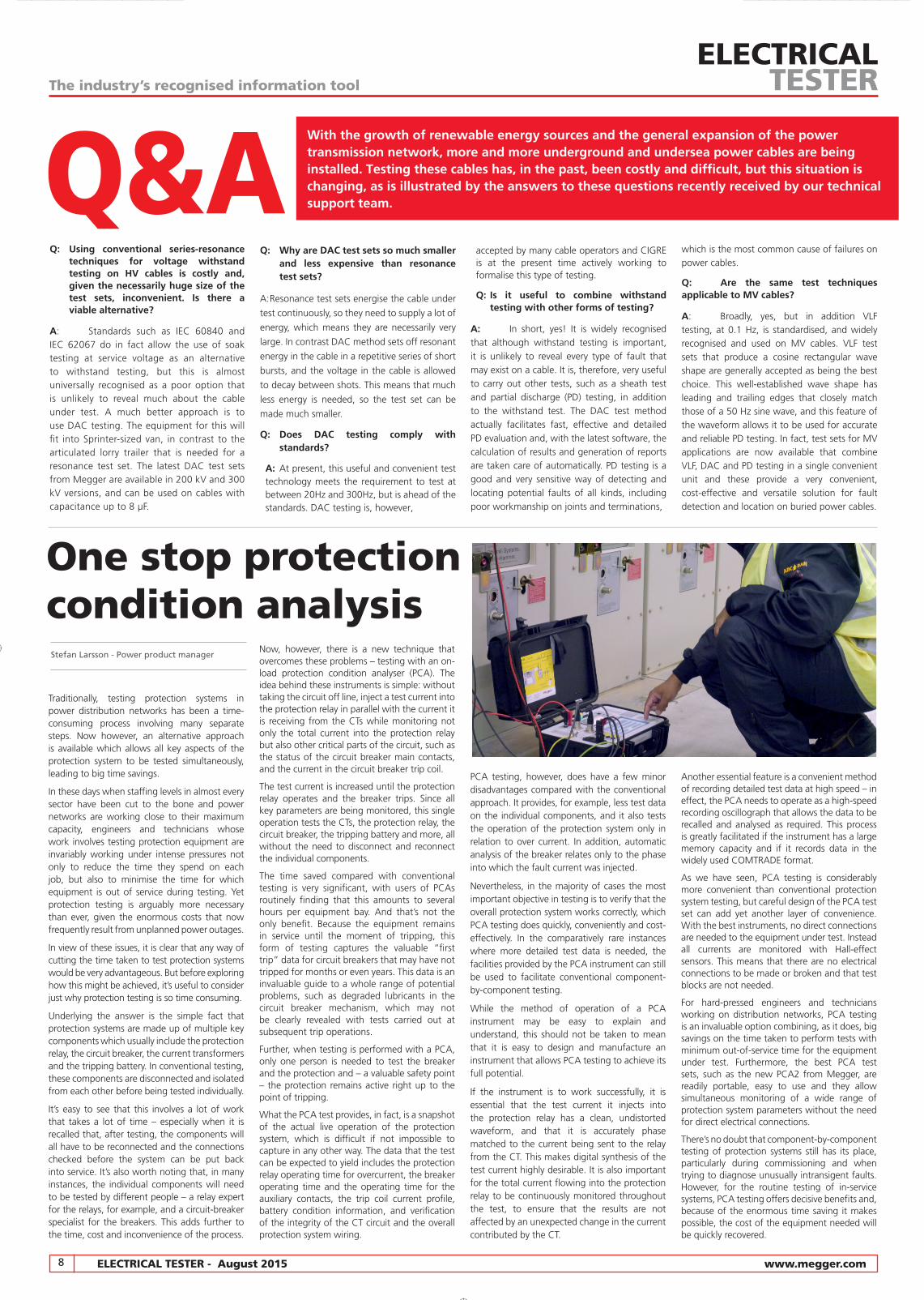
Now, however, there is a new technique that overcomes these problems – testing with an on-load protection condition analyser (PCA). The idea behind these instruments is simple: without taking the circuit off line, inject a test current into the protection relay in parallel with the current it is receiving from the CTs while monitoring not only the total current into the protection relay but also other critical parts of the circuit, such as the status of the circuit breaker main contacts, and the current in the circuit breaker trip coil.

The test current is increased until the protection relay operates and the breaker trips. Since all key parameters are being monitored, this single operation tests the CTs, the protection relay, the circuit breaker, the tripping battery and more, all without the need to disconnect and reconnect the individual components.

The time saved compared with conventional testing is very significant, with users of PCAs routinely finding that this amounts to several hours per equipment bay. And that’s not the only benefit. Because the equipment remains in service until the moment of tripping, this form of testing captures the valuable “first trip” data for circuit breakers that may have not tripped for months or even years. This data is an invaluable guide to a whole range of potential problems, such as degraded lubricants in the circuit breaker mechanism, which may not be clearly revealed with tests carried out at subsequent trip operations.

Further, when testing is performed with a PCA, only one person is needed to test the breaker and the protection and – a valuable safety point – the protection remains active right up to the point of tripping.

What the PCA test provides, in fact, is a snapshot of the actual live operation of the protection system, which is difficult if not impossible to capture in any other way. The data that the test can be expected to yield includes the protection relay operating time for overcurrent, the breaker operating time and the operating time for the auxiliary contacts, the trip coil current profile, battery condition information, and verification of the integrity of the CT circuit and the overall protection system wiring.

PCA testing, however, does have a few minor disadvantages compared with the conventional approach. It provides, for example, less test data on the individual components, and it also tests the operation of the protection system only in relation to over current. In addition, automatic analysis of the breaker relates only to the phase into which the fault current was injected.

Nevertheless, in the majority of cases the most important objective in testing is to verify that the overall protection system works correctly, which PCA testing does quickly, conveniently and cost-effectively. In the comparatively rare instances where more detailed test data is needed, the facilities provided by the PCA instrument can still be used to facilitate conventional component-by-component testing.

While the method of operation of a PCA instrument may be easy to explain and understand, this should not be taken to mean that it is easy to design and manufacture an instrument that allows PCA testing to achieve its full potential.

If the instrument is to work successfully, it is essential that the test current it injects into the protection relay has a clean, undistorted waveform, and that it is accurately phase matched to the current being sent to the relay from the CT. This makes digital synthesis of the test current highly desirable. It is also important for the total current flowing into the protection relay to be continuously monitored throughout the test, to ensure that the results are not affected by an unexpected change in the current contributed by the CT.

Another essential feature is a convenient method of recording detailed test data at high speed – in effect, the PCA needs to operate as a high-speed recording oscillograph that allows the data to be recalled and analysed as required. This process is greatly facilitated if the instrument has a large memory capacity and if it records data in the widely used COMTRADE format.

As we have seen, PCA testing is considerably more convenient than conventional protection system testing, but careful design of the PCA test set can add yet another layer of convenience. With the best instruments, no direct connections are needed to the equipment under test. Instead all currents are monitored with Hall-effect sensors. This means that there are no electrical connections to be made or broken and that test blocks are not needed.

For hard-pressed engineers and technicians working on distribution networks, PCA testing is an invaluable option combining, as it does, big savings on the time taken to perform tests with minimum out-of-service time for the equipment under test. Furthermore, the best PCA test sets, such as the new PCA2 from Megger, are readily portable, easy to use and they allow simultaneous monitoring of a wide range of protection system parameters without the need for direct electrical connections.

There’s no doubt that component-by-component testing of protection systems still has its place, particularly during commissioning and when trying to diagnose unusually intransigent faults. However, for the routine testing of in-service systems, PCA testing offers decisive benefits and, because of the enormous time saving it makes possible, the cost of the equipment needed will be quickly recovered.

Q&AQ: Why are DAC test sets so much smaller and less expensive than resonance test sets?

A: Resonance test sets energise the cable under

test continuously, so they need to supply a lot of

energy, which means they are necessarily very

large. In contrast DAC method sets off resonant

energy in the cable in a repetitive series of short

bursts, and the voltage in the cable is allowed

to decay between shots. This means that much

less energy is needed, so the test set can be

made much smaller.

Q: Does DAC testing comply with standards?

A: At present, this useful and convenient test technology meets the requirement to test at between 20Hz and 300Hz, but is ahead of the standards. DAC testing is, however,

accepted by many cable operators and CIGRE is at the present time actively working to formalise this type of testing.

Q: Is it useful to combine withstand testing with other forms of testing?

A: In short, yes! It is widely recognised that although withstand testing is important, it is unlikely to reveal every type of fault that may exist on a cable. It is, therefore, very useful to carry out other tests, such as a sheath test and partial discharge (PD) testing, in addition to the withstand test. The DAC test method actually facilitates fast, effective and detailed PD evaluation and, with the latest software, the calculation of results and generation of reports are taken care of automatically. PD testing is a good and very sensitive way of detecting and locating potential faults of all kinds, including poor workmanship on joints and terminations,

which is the most common cause of failures on power cables.

Q: Are the same test techniques applicable to MV cables?

A: Broadly, yes, but in addition VLF testing, at 0.1 Hz, is standardised, and widely recognised and used on MV cables. VLF test sets that produce a cosine rectangular wave shape are generally accepted as being the best choice. This well-established wave shape has leading and trailing edges that closely match those of a 50 Hz sine wave, and this feature of the waveform allows it to be used for accurate and reliable PD testing. In fact, test sets for MV applications are now available that combine VLF, DAC and PD testing in a single convenient unit and these provide a very convenient, cost-effective and versatile solution for fault detection and location on buried power cables.

Q: Using conventional series-resonance techniques for voltage withstand testing on HV cables is costly and, given the necessarily huge size of the test sets, inconvenient. Is there a viable alternative?

A: Standards such as IEC 60840 and IEC 62067 do in fact allow the use of soak testing at service voltage as an alternative to withstand testing, but this is almost universally recognised as a poor option that is unlikely to reveal much about the cable under test. A much better approach is to use DAC testing. The equipment for this will fit into Sprinter-sized van, in contrast to the articulated lorry trailer that is needed for a resonance test set. The latest DAC test sets from Megger are available in 200 kV and 300 kV versions, and can be used on cables with capacitance up to 8 µF.

Stefan Larsson - Power product manager

With the growth of renewable energy sources and the general expansion of the power transmission network, more and more underground and undersea power cables are being installed. Testing these cables has, in the past, been costly and difficult, but this situation is changing, as is illustrated by the answers to these questions recently received by our technical support team.

One stop protection condition analysis


Published by Megger August 2015 ELECTRICAL TESTER · ELECTRICAL TESTER ... Published by Megger...

Documents

Transcript of Published by Megger August 2015 ELECTRICAL TESTER · ELECTRICAL TESTER ... Published by Megger...