Projectors on the Generalized Eigenspaces for Partial...

Fields Institute CommunicationsVolume 00, 0000

Projectors on the Generalized Eigenspaces for PartialDifferential Equations with Time Delay

Arnaut DucrotInstitut de Mathematiques de Bordeaux UMR CNRS 5251 & INRIA sud-ouest Anubis,

Universite Victor Segalen Bordeaux 2,3ter place de la victoire, Bat E 2 eme etage, 33076 Bordeaux, France

[email protected]

Pierre MagalInstitut de Mathematiques de Bordeaux UMR CNRS 5251 & INRIA sud-ouest Anubis,

Universite Victor Segalen Bordeaux 2,3ter place de la victoire, Bat E 2 eme etage, 33076 Bordeaux, France

[email protected]

Shigui RuanDepartment of Mathematics, University of Miami,

Coral Gables, FL 33124-4250, [email protected]

Abstract. To study the nonlinear dynamics, such as Hopf bifurcation,of partial differential equations with delay, one needs to consider thecharacteristic equation associated to the linearized equation and to de-termine the distribution of the eigenvalues; that is, to study the spec-trum of the linear operator. In this paper we study the projectors on thegeneralized eigenspaces associated to some eigenvalues for linear partialdifferential equations with delay. We first rewrite partial differentialequations with delay as non-densely defined semilinear Cauchy prob-lems, then obtain formulas for the integrated solutions of the semilinearCauchy problems with non-dense domain by using integrated semigrouptheory, from which we finally derive explicit formulas for the projectorson the generalized eigenspaces associated to some eigenvalues. As exam-ples, we apply the obtained results to study a reaction-diffusion equationwith delay and an age-structured model with delay.

1 Introduction

Taking the interactions of spatial diffusion and time delay into account, a singlespecies population model can be described by a partial differential equation with

1991 Mathematics Subject Classification. Primary 35K57, 34K15; Secondary 92D30.Research of S. Ruan was partially supported by NSF grant DMS-1022728.

c©0000 American Mathematical Society

1

2 Arnaut Ducrot, Pierre Magal, and Shigui Ruan

time delay as follows:

∂u(t, x)∂t

= d∂2u(t, x)

∂x2− au(t− r, x)[1 + u(t, x)], t > 0, x ∈ [0, π] ,

∂u(t, x)∂x

= 0, x = 0, π,

u(0, .) = u0 ∈ C ([0, π] ,R) ,

(1.1)

where u(t, x) denotes the density of the species at time t and location x, d > 0 is thediffusion rate of the species, r > 0 is the time delay constant, and a > 0 is a constant.Equation (1.1) has been studied by many researchers, for example, Yoshida [55],Memory [36], and Busenberg and Huang [12] investigated Hopf bifurcation of theequation.

We consider the Banach space Y = C ([0, π] ,R) endowed with the usual supre-mum norm. Define B : D(B) ⊂ Y → Y by

Bϕ = ϕ′′

withD(B) =

ϕ ∈ C2 ([0, π] ,R) : ϕ′(0) = ϕ′ (π) = 0

.

DenoteL(y) = −ay(−r), f(y) = −ay(0)y(−r).

Equation (1.1) can be written as an abstract partial functional differential equations(PFDE) (see, for example, Travis and Webb [48, 49], Wu [54] and Faria [18]):

dy(t)dt

= By(t) + L(yt) + f(t, yt), ∀t ≥ 0,

y0 = ϕ ∈ CB ,(1.2)

whereCB := ϕ ∈ C ([−r, 0] ; Y ) : ϕ(0) ∈ D(B),

yt ∈ CB satisfies yt (θ) = y (t + θ) , θ ∈ [−r, 0], L : CB → Y is a bounded linearoperator, and f : R × CB → Y is a continuous map. In fact, many other partialdifferential equations with time delay can also be written in the form of system(1.2) (see Wu [54]).

In the last 30 years, partial functional differential equations have been studiedextensively by many researchers. For example, Travis and Webb [48, 49], Fitzgibbon[20], Martin and Smith [30, 31], Arino and Sanchez [8] investigated the fundamentaltheory; Parrot [38] considered the linearized stability; Memory [37] studied thestable and unstable manifolds; Lin et al. [27], Faria et al. [19] and Adimy et al. [4]established the existence and smoothness of center manifolds; Faria [18] developedthe normal form theory; Ruan et al. [41] and Ruan and Zhang [42] discussed thehomoclinic bifurcation. For more detailed theories and results, we refer to themonograph of Wu [54].

In order to study the dynamics of system (1.2), such as Hopf bifurcation, weneed to consider the characteristic equation associated to the linearized equationand to determine the distribution of the eigenvalues; i.e., to carry out the spectrumanalysis of the linear operator. The aim of this article is to obtain explicit formulasfor the projectors on the generalized eigenspaces associated to some eigenvalues forthe linear partial functional differential equation (PFDE)

dy(t)dt

= By(t) + L (yt) ,∀t ≥ 0

y0 = ϕ ∈ CB .(1.3)

Projectors on the Generalized Eigenspaces for PDEs with Time Delay 3

In the context of ordinary functional differential equations with Y = Rn (and Bis bounded), this problem has been studied since the 1970s (see Hale and VerduynLunel [22]), the usual approach is based on the formal adjoint system. The methodwas recently further studied in the monograph of Diekmann et al. [14] using the socalled sun star adjoint spaces, see also Kaashoek and Verduyn Lunel [24], Frassonand Verduyn Lunel [21], Diekmann et al. [13] and the references cited therein. Werefer to Liu et al. [28] for a more recent study on this topic. Let us also mentionthat the explicit formula for the projectors on the generalized eigenspaces turns tobe a crucial tool to study the bifurcations by using normal form arguments (see Liuet al [29] in the context of abstract non-densely defined Cauchy problems).

There are a few approaches to treat problem (1.2). Webb [51] and Travis andWebb [48, 49] viewed the problem as a nonlinear Cauchy problem and focused onmany aspects using this approach. Arino and Sanchez [9] and Kappel [25] usedthe variation of constant formula and worked directly with the system. See alsoRuess [43, 44], Rhandi [40] and the references cited therein. We would like to pointout that the results and techniques in the above mentioned papers do not applydirectly to our problem, as we are not discussing the existence and local stability ofsolutions for linear partial differential equations with delay. Instead, we study theprojectors on the generalized eigenspaces associated to some eigenvalues for linearpartial differential equations with delay so that we can study bifurcations in suchequations. Recently, Adimy [1, 2], Adimy and Arino [3], and Thieme [45] employedthe integrated semigroup theory (see Ezzinbi and Adimy [17] for a survey). Here weuse a formulation that is between the formulations of Adimy [1, 2] and Thieme [45]and more closely related to the one of Travis and Webb [48, 49]. See also Adimyet al. [4].

The rest of the paper is organized as follows. In section 2 we will show howto formulate the partial functional differential equation as a semilinear Cauchyproblem with non-dense domain. In section 3 we recall some results on integratedsemigroup theory and spectrum analysis. Section 4 presents main results on projec-tors on the eiganspaces. Section 5 deals with a special case for a simple eiganvalue.Some examples and discussions are given in section 6.

2 Preliminaries

Let B : D(B) ⊂ Y → Y be a linear operator on a Banach space (Y, ‖ ‖Y ).Assume that it is a Hille-Yosida operator; that is, there exist two constants, ωB ∈ Rand MB > 0, such that (ωB , +∞) ⊂ ρ (B) and

∥∥∥(λI −B)−n∥∥∥ ≤ MB

(λ− ωB)n , ∀λ > ωB , ∀n ≥ 1.

SetY0 := D(B).

Consider B0, the part of B in Y0, which is defined by

B0y = By for each y ∈ D (B0)

withD (B0) := y ∈ D(B) : By ∈ Y0 .

For r ≥ 0, setC := C ([−r, 0] ; Y )


which is endowed with the supremum norm

‖ϕ‖∞ = supθ∈[−r,0]

‖ϕ (θ)‖Y .

Consider the partial functional differential equations (PFDE):

dy(t)dt

= By(t) + L(yt) + f(t, yt), ∀t ≥ 0,

y0 = ϕ ∈ CB ,(2.1)

where yt ∈ CB satisfies yt (θ) = y (t + θ) , θ ∈ [−r, 0], L : CB → Y is a boundedlinear operator, and f : R×CB → Y is a continuous map. Since B is a Hille-Yosidaoperator, it is well known that B0, the part of B in Y0, generates a C0-semigroupof bounded linear operators TB0(t)t≥0 on Y0, and B generates an integratedsemigroup SB(t)t≥0 on Y . The solution of the Cauchy problem (2.1) must beunderstood as a fixed point of

y(t) = TB0(t)ϕ(0) +d

dt

∫ t

0

SB(t− s)[L(ys) + f(s, ys)

]ds.

Since TB0(t)t≥0 acts on Y0, we observe that it is necessary to assume that

ϕ(0) ∈ Y0 ⇒ ϕ ∈ CB .

In order to study the PFDE (2.1) by using the integrated semigroup theory, we con-sider the PFDE (2.1) as an abstract non-densely defined Cauchy problem. Firstly,we regard the PFDE (2.1) as a PDE. Define u ∈ C ([0, +∞)× [−r, 0] , Y ) by

u (t, θ) = y(t + θ), ∀t ≥ 0, ∀θ ∈ [−r, 0] .

Note that if y ∈ C1 ([−r,+∞) , Y ) , then

∂u(t, θ)∂t

= y′(t + θ) =∂u(t, θ)

∂θ.

Hence, we must have∂u(t, θ)

∂t− ∂u(t, θ)

∂θ= 0, ∀t ≥ 0, ∀θ ∈ [−r, 0] .

Moreover, for θ = 0, we obtain∂u(t, 0)

∂θ= y′(t) = By(t)+L(yt)+f(t, yt) = Bu(t, 0)+L(u(t, .))+f(t, u(t, .)), ∀t ≥ 0.

Therefore, we deduce formally that u must satisfy a PDE

∂u(t, θ)∂t

− ∂u(t, θ)∂θ

= 0,

∂u(t, 0)∂θ

= Bu(t, 0) + L(u(t, .)) + f(t, u(t, .)), ∀t ≥ 0,

u(0, .) = ϕ ∈ CB .

(2.2)

In order to rewrite the PDE (2.2) as an abstract non-densely defined Cauchy prob-lem, we extend the state space to take into account the boundary conditions. Thiscan be accomplished by adopting the following state space

X = Y × C

taken with the usual product norm∥∥∥∥(

yϕ

)∥∥∥∥ = ‖y‖Y + ‖ϕ‖∞ .


Define the linear operator A : D(A) ⊂ X → X by

A

(0Y

ϕ

)=

( −ϕ′(0) + Bϕ(0)ϕ′

), ∀

(0Y

ϕ

)∈ D(A) (2.3)

withD(A) = 0Y × ϕ ∈ C1 ([−r, 0] , Y ) , ϕ(0) ∈ D(B).

Note that A is non-densely defined because

X0 := D(A) = 0Y × CB 6= X.

We also define L : X0 → X by

L

(0Y

ϕ

):=

(L (ϕ)0C

)

and F : R×X0 → X by

F

(t,

(0Y

ϕ

)):=

(f(t, ϕ)

0C

).

Set

v(t) :=(

0Y

u(t)

).

Now we can consider the PDE (2.2) as the following non-densely defined Cauchyproblem

dv(t)dt

= Av(t) + L(v(t)) + F (t, v(t)), t ≥ 0; v(0) =(

0Y

ϕ

)∈ X0. (2.4)

3 Some results on integrated solutions and spectra

In this section we will first study the integrated solutions of the Cauchy problem(2.4) in the special case

dv(t)dt

= Av(t) +(

h(t)0

), t ≥ 0, v(0) =

(0Y

ϕ

)∈ X0, (3.1)

where h ∈ L1 ((0, τ) , Y ). Recall that v ∈ C ([0, τ ] , X) is an integrated solution of(3.1) if and only if ∫ t

0

v(s)ds ∈ D(A),∀t ∈ [0, τ ] (3.2)

and

v(t) =(

0Y

ϕ

)+ A

∫ t

0

v(s)ds +∫ t

0

(h(s)0

)ds. (3.3)

In the sequel, we will use the integrated semigroup theory to define such an inte-grated solution. We refer to Arendt [5], Thieme [46], Kellermann and Hieber [26],and the book of Arendt et al. [6] for further details on this subject. We also referto Magal and Ruan [33, 34, 35] for more results and update references.

From (3.2) we note that if v is an integrated solution we must have

v(t) = limh→0+

1h

∫ t+h

t

v(s)ds ∈ D(A).

Hence

v(t) =(

0Y

u(t)

)


withu ∈ C ([0, τ ] , CB) .

We introduce some notations. Let L : D(L) ⊂ X → X be a linear operator on acomplex Banach space X. Denote by ρ(L) the resolvent set of L,N(L) the null spaceof L, and R(L) the range of L, respectively. The spectrum of L is σ (L) = C\ρ (L) .The point spectrum of L is the set

σP (L) := λ ∈ C : N (λI − L) 6= 0 .

The essential spectrum (in the sense of Browder [11]) of L is denoted by σess (L) .That is, the set of λ ∈ σ (L) such that at least one of the following holds: (i) R(λI−L) is not closed; (ii) λ is a limit point of σ (L) ; (iii) Nλ(L) :=

⋃∞k=1 N

((λI − L)k

)

is infinite dimensional. Define

Xλ0 =⋃

n≥0

N ((λ0 − L)n) .

Let Y be a subspace of X. Then we denote by LY : D(LY ) ⊂ Y → Y the part ofL on Y , which is defined by

LY y = Ly, ∀y ∈ D (LY ) := y ∈ D(L) ∩ Y : Ly ∈ Y .

Definition 3.1 Let L : D(L) ⊂ X → X be the infinitesimal generator of alinear C0-semigroup TL(t)t≥0 on a Banach space X. We define the growth boundω0 (L) ∈ [−∞, +∞) of L by

ω0 (L) := limt→+∞

ln(‖TL(t)‖L(X)

)

t.

The essential growth bound ω0,ess (L) ∈ [−∞, +∞) of L is defined by

ω0,ess (L) := limt→+∞

ln (‖TL(t)‖ess)t

,

where ‖TL(t)‖ess is the essential norm of TL(t) defined by

‖TL(t)‖ess = κ (TL(t)BX (0, 1)) ,

here BX (0, 1) = x ∈ X : ‖x‖X ≤ 1 , and for each bounded set B ⊂ X,

κ (B) = inf ε > 0 : B can be covered by a finite number of balls of radius ≤ εis the Kuratovsky measure of non-compactness.

We have the following result. The existence of the projector was first proved byWebb [52, 53] and the fact that there is a finite number of points of the spectrumis proved by Engel and Nagel [16, Corollary 2.1, p. 258].

Theorem 3.2 Let L : D(L) ⊂ X → X be the infinitesimal generator of alinear C0-semigroup TL(t) on a Banach space X. Then

ω0 (L) = max(

ω0,ess (L) , maxλ∈σ(L)\σess(L)

Re (λ))

.

Assume in addition that ω0,ess (L) < ω0 (L) . Then for each γ ∈ (ω0,ess (L) , ω0 (L)] ,λ ∈ σ (L) : Re (λ) ≥ γ ⊂ σp(L) is nonempty, finite and contains only poles ofthe resolvent of L. Moreover, there exists a finite rank bounded linear operator ofprojection Π : X → X satisfying the following properties:

(a) Π (λ− L)−1 = (λ− L)−1 Π,∀λ ∈ ρ (L) ;


(b) σ(LΠ(X)

)= λ ∈ σ (L) : Re (λ) ≥ γ ;

(c) σ(L(I−Π)(X)

)= σ (L) \ σ

(LΠ(X)

).

In Theorem 3.2 the projector Π is the projection on the direct sum of thegeneralized eigenspaces of L associated to all points λ ∈ σ (L) with Re (λ) ≥ γ. Asa consequence of Theorem 3.2 we have following corollary.

Corollary 3.3 Let L : D(L) ⊂ X → X be the infinitesimal generator of alinear C0-semigroup TL(t) on a Banach space X, and assume that ω0,ess (L) <ω0 (L) . Then

λ ∈ σ (L) : Re (λ) > ω0,ess (L) ⊂ σP (L)

and each λ ∈ λ ∈ σ (L) : Re (λ) > ω0,ess (L) is a pole of the resolvent of L. Thatis, λ is isolated in σ (L) , and there exists an integer k0 ≥ 1 (the order of the pole)such that the Laurent’s expansion of the resolvent takes the following form

(λI − L)−1 =∞∑

n=−k0

(λ− λ0)n

Bλ0n ,

where Bλ0n are bounded linear operators on X, and the above series converges in

the norm of operators whenever |λ− λ0| is small enough.

The following result is due to Magal and Ruan [35, see Lemma 2.1 and Propo-sition 3.6].

Theorem 3.4 Let (X, ‖.‖) be a Banach space and L : D(L) ⊂ X → X bea linear operator. Assume that ρ (L) 6= ∅ and L0, the part of L in D(L), is theinfinitesimal generator of a linear C0-semigroup TL0(t)t≥0 on the Banach spaceD(L). Then

σ (L) = σ (L0) .

Let X0 := D(L), Π0 : D(L) → D(L) be a bounded linear operator of projection.Assume that

Π0 (λI − L0)−1 = (λI − L0)

−1 Π0, ∀λ > ω

andΠ0

(D(L)

)⊂ D(L0) and L0 |Π0(D(L)) is bounded.

Then there exists a unique bounded linear operator of projection Π on X satisfyingthe following properties:

(i) Π |D(L)

= Π0.

(ii) Π (X) ⊂ D(L).(iii) Π (λI − L)−1 = (λI − L)−1 Π,∀λ > ω.

Moreover, for each x ∈ X we have the following approximation formula

Πx = limλ→+∞

Π0λ (λI − L)−1x.

We return to the Cauchy problem (3.1) and investigate some properties of thelinear operator A.

Theorem 3.5 For the operator A defined in (2.3), the resolvent set of A sat-isfies

ρ (A) = ρ (B) .


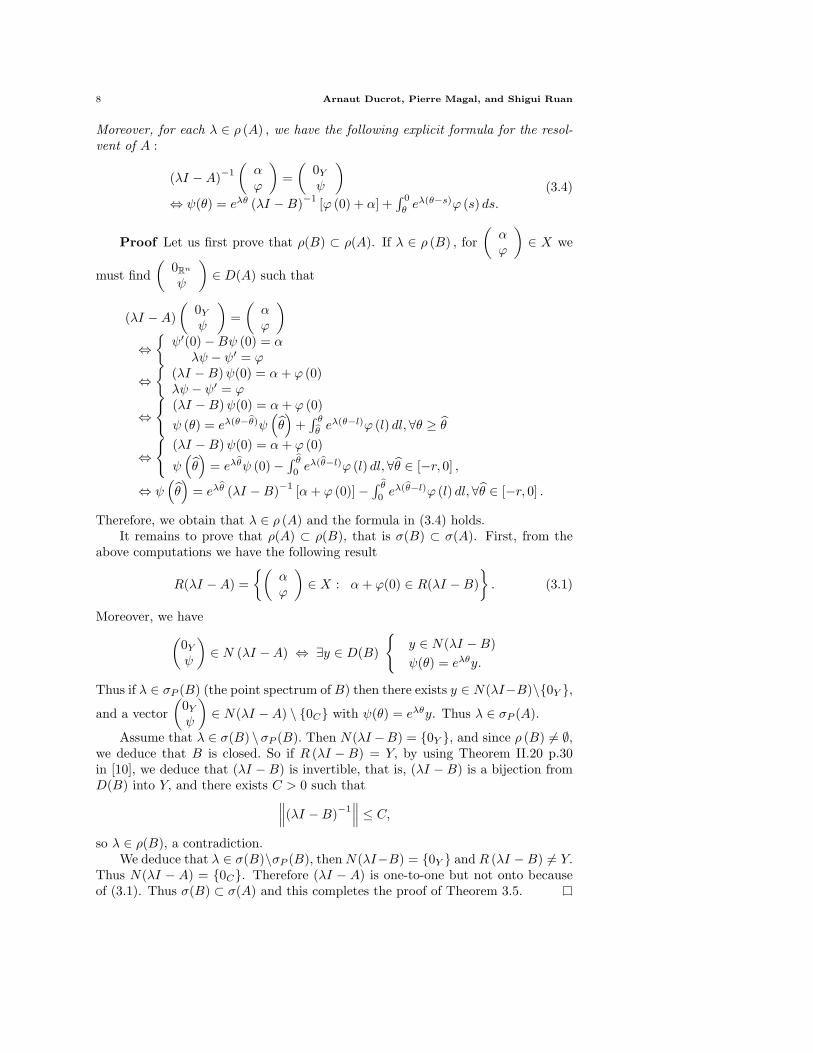
Moreover, for each λ ∈ ρ (A) , we have the following explicit formula for the resol-vent of A :

(λI −A)−1

(αϕ

)=

(0Y

ψ

)

⇔ ψ(θ) = eλθ (λI −B)−1 [ϕ (0) + α] +∫ 0

θeλ(θ−s)ϕ (s) ds.

(3.4)

Proof Let us first prove that ρ(B) ⊂ ρ(A). If λ ∈ ρ (B) , for(

αϕ

)∈ X we

must find(

0Rn

ψ

)∈ D(A) such that

(λI −A)(

0Y

ψ

)=

(αϕ

)

⇔

ψ′(0)−Bψ (0) = αλψ − ψ′ = ϕ

⇔

(λI −B)ψ(0) = α + ϕ (0)λψ − ψ′ = ϕ

⇔

(λI −B)ψ(0) = α + ϕ (0)ψ (θ) = eλ(θ−θ)ψ

(θ)

+∫ θ

θeλ(θ−l)ϕ (l) dl, ∀θ ≥ θ

⇔

(λI −B)ψ(0) = α + ϕ (0)

ψ(θ)

= eλθψ (0)− ∫ θ

0eλ(θ−l)ϕ (l) dl, ∀θ ∈ [−r, 0] ,

⇔ ψ(θ)

= eλθ (λI −B)−1 [α + ϕ (0)]− ∫ θ

0eλ(θ−l)ϕ (l) dl, ∀θ ∈ [−r, 0] .

Therefore, we obtain that λ ∈ ρ (A) and the formula in (3.4) holds.It remains to prove that ρ(A) ⊂ ρ(B), that is σ(B) ⊂ σ(A). First, from the

above computations we have the following result

R(λI −A) =(

αϕ

)∈ X : α + ϕ(0) ∈ R(λI −B)

. (3.1)

Moreover, we have(

0Y

ψ

)∈ N (λI −A) ⇔ ∃y ∈ D(B)

y ∈ N(λI −B)ψ(θ) = eλθy.

Thus if λ ∈ σP (B) (the point spectrum of B) then there exists y ∈ N(λI−B)\0Y ,and a vector

(0Y

ψ

)∈ N(λI −A) \ 0C with ψ(θ) = eλθy. Thus λ ∈ σP (A).

Assume that λ ∈ σ(B) \σP (B). Then N(λI −B) = 0Y , and since ρ (B) 6= ∅,we deduce that B is closed. So if R (λI −B) = Y, by using Theorem II.20 p.30in [10], we deduce that (λI −B) is invertible, that is, (λI −B) is a bijection fromD(B) into Y, and there exists C > 0 such that

∥∥∥(λI −B)−1∥∥∥ ≤ C,

so λ ∈ ρ(B), a contradiction.We deduce that λ ∈ σ(B)\σP (B), then N(λI−B) = 0Y and R (λI −B) 6= Y.

Thus N(λI − A) = 0C. Therefore (λI − A) is one-to-one but not onto becauseof (3.1). Thus σ(B) ⊂ σ(A) and this completes the proof of Theorem 3.5.


Lemma 3.6 The linear operator A : D(A) ⊂ X → X is a Hille-Yosida opera-tor. More precisely, for each ωA > ωB , there exists MA ≥ 1 such that

∥∥∥(λI −A)−n∥∥∥L(X)

≤ MA

(λ− ωA)n ,∀n ≥ 1, ∀λ > ωA. (3.5)

Proof Let ωA > ωB . Since B is a Hille-Yosida operator on Y , following Lemma5.1 in Pazy [39], we can find an equivalent norm |.|Y on Y such that

∣∣∣(λI −B)−1x∣∣∣ ≤ |x|

λ− ωB∀λ > ωB , ∀x ∈ Y.

Then we define |.| the equivalent norm on X by∣∣∣∣(

αϕ

)∣∣∣∣ = |α|+ ‖ϕ‖ωA,

where‖ϕ‖ωA

:= supθ∈[−r,0]

∣∣e−ωAθϕ (θ)∣∣ .

Using (3.4) and the above results, we obtain for each λ > ωA that∣∣∣∣(λI −A)−1

(αϕ

)∣∣∣∣

≤ supθ∈[−r,0]

[e−ωAθeλθ

∣∣∣(λI −B)−1 [ϕ (0) + α]∣∣∣ + e−ωAθ

∫ 0

θ

eλ(θ−s) |ϕ (s)| ds

]

≤ supθ∈[−r,0]

[e−ωAθeλθ 1

λ− ωB[|ϕ (0)|+ |α|] + e−ωAθeλθ

∫ 0

θ

e−(λ−ωA)sds ‖ϕ‖ωA

]

=1

λ− ωA|α|+ sup

θ∈[−r,0]

[e−ωAθeλθ

λ− ωA|ϕ (0) |+ e−ωAθeλθ

[e−(λ−ωA)θ − 1

]

λ− ωA‖ϕ‖ωA

]

≤ 1λ− ωA

[|α|+ ‖ϕ‖ωA

]

=1

λ− ωA

∣∣∣∣(

αϕ

)∣∣∣∣ .

Therefore, (3.5) holds and the proof is completed.

Since A is a Hille-Yosida operator, A generates a non-degenerated integratedsemigroup SA(t)t≥0 on X. It follows from Thieme [46] and Kellerman and Hieber[26] that the abstract Cauchy problem (3.1) has at most one integrated solution.

Lemma 3.7 Let h ∈ L1 ((0, τ) , Y ) and ϕ ∈ C ([−r, 0] , Y ) with ϕ(0) ∈ Y0.Then there exists an unique integrated solution t → v(t) of the Cauchy problem(3.1) which can be expressed explicitly by the following formula

v(t) =(

0Y

u(t)

)

withu(t) (θ) = y(t + θ), ∀t ∈ [0, τ ] , ∀θ ∈ [−r, 0] , (3.6)

where

y(t) =

ϕ (t) , t ∈ [−r, 0] ,TB0(t)ϕ (0) + (SB ¦ h)(t), t ∈ [0, τ ]


and

(SB ¦ h)(t) :=d

dt(SB ∗ h)(t), (SB ∗ h)(t) :=

∫ t

0

SB(t− s)h(s)ds.

Proof Since A is a Hille-Yosida operator, there is at most one integrated solu-tion of the Cauchy problem (3.1). So it is sufficient to prove that u defined by (3.6)satisfies for each t ∈ [0, τ ] the following

(0Y∫ t

0u(l)dl

)∈ D(A) (3.7)

and (0Y

u(t)

)=

(0Y

ϕ

)+ A

(0Y∫ t

0u(l)dl

)+

( ∫ t

0h(l)dl0

). (3.8)

Since ∫ t

0

u(l) (θ) dl =∫ t

0

y(l + θ)dl =∫ t+θ

θ

y(s)ds

and y ∈ C ([−r, τ ] , Y ) , the map θ → ∫ t

0u(l) (θ) dl belongs to C1 ([−r, 0] , Y ) . We

also observe that∫ t

0

u(l) (0) dl =∫ t

0

y (l) dl =∫ t

0

TB0(l)ϕ (0) + (SB ¦ h)(l)dl

=∫ t

0

TB0(l)ϕ (0) dl + (SB ∗ h)(t) ∈ D(B),

therefore, (3.7) follows. Moreover,

A

(0Y

ϕ

)=

( −ϕ′(0) + Bϕ(0)ϕ′

)

whenever ϕ ∈ C1 ([−r, 0] , Y ) with ϕ(0) ∈ D(B). Hence

A

(0∫ t

0u(l)dl

)=

(− [y(t)− y(0)] + B

∫ t

0y(s)ds

[y(t + .)− y(.)]

)

= −(

0ϕ

)+

(− [y(t)− ϕ(0)] + B

∫ t

0y(s)ds

y(t + .)

).

Therefore, (3.8) is satisfied if and only if

y(t) = ϕ(0) + B

∫ t

0

y(s)ds +∫ t

0

h(s)ds. (3.9)

Since B is a Hille-Yosida operator, we deduce that (3.9) is equivalent to

y(t) = TB0(t)ϕ(0) + (SB ¦ h)(t).

The proof is completed.

Recall that A0 : D (A0) ⊂ D(A) → D(A), the part of A in D(A), is defined by

A0

(0Y

ϕ

)= A

(0Y

ϕ

),∀

(0Y

ϕ

)∈ D (A0) ,

where

D (A0) =(

0Y

ϕ

)∈ D (A) : A

(0Y

ϕ

)∈ D(A)

.


From the definition of A in (2.3) and the fact that

D(A) = 0Y × ϕ ∈ C ([−r, 0] , Y ) , ϕ(0) ∈ Y0,we know that A0 is a linear operator defined by

A0

(0Y

ϕ

)=

(0Y

ϕ′

), ∀

(0Y

ϕ

)∈ D (A0) ,

whereD (A0)

=(

0Y

ϕ

)∈ 0Y × ϕ ∈ C1 ([−r, 0] , Y ) : ϕ(0) ∈ D(B), −ϕ′(0) + Bϕ(0) = 0

.

Now by using the fact that A is a Hille-Yosida operator, we deduce that A0 is theinfinitesimal generator of a strongly continuous semigroup TA0(t)t≥0 and

v(t) = TA0(t)(

0Y

ϕ

)

is an integrated solution ofdv(t)dt

= Av(t), t ≥ 0, v(0) =(

0Y

ϕ

)∈ X0.

Using Lemma 3.7 with h = 0, we obtain the following result.

Lemma 3.8 The linear operator A0 is the infinitesimal generator of a stronglycontinuous semigroup TA0(t)t≥0 of bounded linear operators on D(A) which isdefined by

TA0(t)(

0Y

ϕ

)=

(0Y

TA0(t) (ϕ)

), (3.10)

where

TA0(t) (ϕ) (θ) =

TB0 (t + θ)ϕ (0) , t + θ ≥ 0,ϕ(t + θ), t + θ ≤ 0.

Since A is a Hille-Yosida operator, we know that A generates an integrated

semigroup SA(t)t≥0 on X, and t → SA(t)(

yϕ

)is an integrated solution of

dv(t)dt

= Av(t) +(

yϕ

), t ≥ 0, v(0) = 0.

Since SA (t) is linear we have

SA(t)(

yϕ

)= SA(t)

(0Y

ϕ

)+ SA(t)

(y0C

),

where

SA(t)(

0Y

ϕ

)=

∫ t

0

TA0(l)(

0Y

ϕ

)dl

and SA(t)(

y0

)is an integrated solution of

dv(t)dt

= Av(t) +(

y0

), t ≥ 0, v(0) = 0.

Therefore, by using Lemma 3.7 with h(t) = y and the above results, we obtain thefollowing result.


Lemma 3.9 The linear operator A generates an integrated semigroup SA(t)t≥0

on X. Moreover,

SA(t)(

yϕ

)=

(0Y

SA(t) (y, ϕ)

),

(yϕ

)∈ X,

where SA(t) is the linear operator defined by

SA(t) (y, ϕ) = SA(t) (0, ϕ) + SA(t) (y, 0)

with

SA(t) (0, ϕ) (θ) =∫ t

0

TA0(s)(ϕ) (θ) ds =∫ t

−θ

TB0(s + θ)ϕ(0)ds +∫ −θ

0

ϕ(s + θ)ds

and

SA(t) (y, 0) (θ) =

SB(t + θ)y, t + θ ≥ 0,0, t + θ ≤ 0.

Now we focus on the spectra of A and A+L. Since A is a Hille-Yosida operator,so is A + L. Moreover, (A + L)0 : D((A + L)0) ⊂ D(A) → D(A), the part of A + L

in D(A), is a linear operator defined by

(A + L)0

(0Y

ϕ

)=

(0Y

ϕ′

), ∀

(0Y

ϕ

)∈ D ((A + L)0) ,

whereD ((A + L)0) =(

0Y

ϕ

)∈ 0Y × ϕ ∈ C1 ([−r, 0] , Y ) : ϕ(0) ∈ D(B), ϕ′(0) = Bϕ(0) + L (ϕ)

.

From Theorems 3.4 and 3.5, we know that

σ (B) = σ (A) = σ (A0) and σ (A + L) = σ ((A + L)0) .

From (3.10), we have

TA0(t) (ϕ) (θ) = TB0 (r + θ)TB0 (t− r)ϕ (0) , t ≥ r, θ ∈ [−r, 0] .

Therefore we getω0,ess(A0) ≤ ω0,ess(B0). (3.2)

In the following lemma, we specify the essential growth rate of the C0-semigroupgenerated by (A + L)0 in some cases. Unfortunately, this problem is not fully un-derstood.

Lemma 3.10 Assume that one of the two following properties are satisfied:

(a) For each t > 0, LTA0(t) is compact from C into Y.(b) For each t > 0, TB0(t) is compact on Y.

Then we haveω0,ess((A + L)0) ≤ ω0,ess(B0).

Proof For Assumption (a) the result is a direct consequence of Theorem 1.2in Ducrot et al. [15] or the results in Thieme [47]. The case (b) has been treatedby Adimy et al. [4, Theorem 2.7].


From now on we set

Ω = λ ∈ C : Re (λ) > ω0,ess((A + L)0).From the discussion in this section, we obtain the following proposition.

Proposition 3.11 The linear operator A + L : D(A) ⊂ X → X is a Hille-Yosida operator. (A + L)0 is the infinitesimal generator of a strongly continuoussemigroup

T(A+L)0

(t)

t≥0of bounded linear operators on D(A). Moreover,

T(A+L)0(t)

(0Y

ϕ

)=

(0Y

T(A+L)0(t) (ϕ)

)(3.15)

withT(A+L)0

(t) (ϕ) (θ) = y(t + θ), ∀t ≥ 0, ∀θ ∈ [−r, 0] ,where

y(t) =

ϕ(t), ∀t ∈ [−r, 0] ,TB0(t)ϕ(0) +

(SB ¦ L (y.)

)(t), ∀t ≥ 0.

Furthermore, we have that

σ((A + L)0) ∩ Ω = σP ((A + L)0) ∩ Ω = λ ∈ Ω : N (∆(λ)) 6= 0,where ∆(λ) : D(B) ⊂ Y → Y is the following linear operator

∆(λ) = λI −B − L(eλ.IY

). (3.11)

Then each λ0 ∈ σ ((A + L)0) ∩ Ω is a pole in Ω of (λI − (A + L))−1. For each

γ > ω0,ess((A + L)0), the subset λ ∈ σ ((A + L)0) : Re (λ) ≥ γ is either empty orfinite.

Proof The first part of the result follows immediately from Lemma 3.7 ap-plied with h(t) = L (yt), and the last part of the proof follows from Theorem 3.2,Corollary 3.3, and Theorem 3.4.

4 Projectors on the eigenspaces

Let λ0 ∈ σ (A + L) ∩ Ω. From the above discussion we already knew that λ0

is a pole of (λI − (A + L))−1 of finite order k0 ≥ 1. This means that λ0 is isolatedin σ (A + L) and the Laurent’s expansion of the resolvent around λ0 takes thefollowing form

(λI − (A + L))−1 =+∞∑

n=−k0

(λ− λ0)n

Bλ0n . (4.1)

The bounded linear operator Bλ0−1 is the projector on the generalized eigenspace of

(A + L) associated to λ0. The goal of this section is to provide a method to computeBλ0−1. We remark that

(λ− λ0)k0 (λI − (A + L))−1 =

+∞∑m=0

(λ− λ0)m

Bλ0m−k0

.

So we have the following approximation formula

Bλ0−1 = lim

λ→λ0

1(k0 − 1)!

dk0−1

dλk0−1

((λ− λ0)

k0 (λI − (A + L))−1)

. (4.2)


In order to compute an explicit formula for the resolvent of A + L we will usethe following lemma.

Lemma 4.1 Let A : D(A) ⊂ X → X be a linear operator on a Banach spaceX with ρ (A) 6= ∅. Let B : D(A) → X be a bounded linear operator. Then for eachλ ∈ ρ (A) we have

λ ∈ ρ (A + B) ⇔ 1 ∈ ρ(B (λI −A)−1

).

Moreover, for each λ ∈ ρ (A + B) we have

(λI −A−B)−1 = (λI −A)−1[I −B (λI −A)−1

]−1

[I −B (λI −A)−1

]−1

= I + B (λI −A−B)−1

Proof Assume first that 1 ∈ ρ(B (λI −A)−1

). Then

(λI −A−B) (λI −A)−1[I −B (λI −A)−1

]−1

=[I −B (λI −A)−1

] [I −B (λI −A)−1

]−1

= I,

and

(λI −A)−1[I −B (λI −A)−1

]−1

(λI −A−B)

= (λI −A)−1[I −B (λI −A)−1

]−1 (I −B (λI −A)−1

)(λI −A)

= ID(A).

Thus λ ∈ ρ (A + B) , and

(λI −A−B)−1 = (λI −A)−1[I −B (λI −A)−1

]−1

.

Conversely, assume that λ ∈ ρ (A + B) , then[I −B (λI −A)−1

] [I + B (λI −A−B)−1

]

=[I −B (λI −A)−1

] [(λI −A−B) (λI −A−B)−1 + B (λI −A−B)−1

]

=[I −B (λI −A)−1

] [(λI −A) (λI −A−B)−1

]

= (λI −A) (λI −A−B)−1 −B (λI −A−B)−1 = I

and [I + B (λI −A−B)−1

] [I −B (λI −A)−1

]

=[(λI −A) (λI −A−B)−1

] [I −B (λI −A)−1

]

= (λI −A) (λI −A−B)−1 [λI −A−B] (λI −A)−1

= I.

Thus, 1 ∈ ρ(B (λI −A)−1

)and

[I −B (λI −A)−1

]−1

= I + B (λI −A−B)−1.


This completes the proof.

In order to give an explicit formula for Bλ0−1, we need the following results.

Lemma 4.2 We have the following equivalence:

λ ∈ ρ (A + L) ∩ Ω ⇔ ∆(λ) is invertible.

Moreover, we have the following explicit formula for the resolvent of A + L

(λI − (A + L))−1

(αϕ

)=

(0Y

ψ

)

⇔ψ (θ) =

∫ 0

θeλ(θ−s)ϕ (s) ds + eλθ∆ (λ)−1

[α + ϕ (0) + L

(∫ 0

.eλ(.−s)ϕ (s) ds

)].

(4.3)

Proof We consider the linear operator Aγ : D(A) ⊂ X → X defined by

Aγ

(0Y

ϕ

)=

( −ϕ′(0) + (B − γI)ϕ(0)ϕ′

), ∀

(0Y

ϕ

)∈ D(A),

and

Lγ

(0Y

ϕ

)=

(L (ϕ) + γϕ(0)

0C

).

Then we haveA + L = Aγ + Lγ .

Moreover,ω0 (B0 − γI) = ω0 (B0)− γ.

Hence by Theorem 3.5, for λ ∈ C with Re (λ) > ω0 (B0) − γ, we have λ ∈ ρ (Aγ)and

(λI −Aγ)−1

(αϕ

)=

(0Y

ψ

)

⇔ ψ(θ) = eλθ (λI − (B − γI))−1 [ϕ (0) + α] +∫ 0

θeλ(θ−s)ϕ (s) ds.

(4.4)

Therefore, for each λ ∈ C with Re (λ) > ω0 (B0)−γ, by Lemma 4.1 we deduce that[λI − (Aγ + Lγ)] is invertible if and only if I − Lγ (λI −Aγ)−1 is invertible, and

(λI − (Aγ + Lγ))−1 = (λI −Aγ)−1[I − Lγ (λI −Aγ)−1

]−1

. (4.5)

We also know that[I − Lγ (λI −Aγ)−1

] (αϕ

)=

(αϕ

)is equivalent to ϕ = ϕ

and

α−[L

(eλ. (λI − (B − γI))−1

α)

+ γ (λI − (B − γI))−1α]

= α +

[L

(eλ. (λI − (B − γI))−1

ϕ (0) +∫ 0


)

+γ (λI − (B − γI))−1ϕ (0)

].

Because

α− L(eλ. (λI − (B − γI))−1

α)− γ (λI − (B − γI))−1

α

=[λI − (B − γI)− L

(eλ.I

)− γI](λI − (B − γI))−1

α

=[λI −B − L

(eλ.I

)](λI − (B − γI))−1

α


= ∆(λ) (λI − (B − γI))−1α

and B is closed, we deduce that ∆ (λ) is closed, and by using the same argumentsas in the proof of Theorem 3.5 to

∆ (λ) (λI − (B − γI))−1α

= α +

[L

(eλ. (λI − (B − γI))−1

ϕ (0) +∫ 0


)

+γ (λI − (B − γI))−1ϕ (0)

]

we deduce that[I − Lγ (λI −Aγ)−1

]is invertible if and only if

∆ (λ) =[λI −B − L

(eλ.I

)]

is invertible. So for λ ∈ Ω, [λI − (A + L)] is invertible if and only if ∆ (λ) isinvertible.

Moreover, [I − Lγ (λI −Aγ)−1

]−1(

αϕ

)=

(αϕ

)

is equivalent to ϕ = ϕ and

α = (λI − (B − γI)) ∆ (λ)−1

[α + L

(eλ. (λI − (B − γI))−1

ϕ (0) +∫ 0


)

+γ (λI − (B − γI))−1ϕ (0)

].

(4.6)Note that A + L = Aγ + Lγ . By using (4.4), (4.5) and (4.6), we obtain for eachγ > 0 large enough that

(λI − (A + L))−1

(αϕ

)=

(0Rn

ψ

)

⇔ψ (θ) = eλθ (λI − (B − γI))−1

ϕ (0) +∫ 0

θeλ(θ−s)ϕ (s) ds

+eλθ∆ (λ)−1

[α + L

(eλ. (λI − (B − γI))−1

ϕ (0) +∫ 0


)

+γ (λI − (B − γI))−1ϕ (0)

],

but

(λI − (B − γI))−1ϕ (0) + ∆ (λ)−1

[L

(eλ.I

)+ γI

](λI − (B − γI))−1

ϕ (0)

=(

I +[λI −B − L

(eλ.I

)]−1 [L

(eλ.I

)+ B − λI + λI − (B − γI)

])

· (λI − (B − γI))−1ϕ (0)

=(

I − I +[λI −B − L

(eλ.I

)]−1

[λI − (B − γI)])

(λI − (B − γI))−1ϕ (0)

=[λI −B − L

(eλ.I

)]−1

ϕ (0)

and the result follows.

Next we introduce the following operators Π : X0 → C and F : Y → X suchthat

Π(

0Y

ϕ

)= ϕ(0), Fα =

(α0C

).

Then from Lemma 4.2 we have:

Π(λI − (A + L))−1Fα = ∆−1(λ)α, ∀λ ∈ ρ(A + L) ∩ Ω, ∀α ∈ Y. (4.7)


Since λ → (λI − (A + L))−1 is holomorphic from Ω into L (X) , we deduce fromthe above formula that the map λ → ∆−1(λ) is holomorphic in Ω. Moreover,by Proposition 3.11 we know that ∆−1(.) has only finite order poles. Therefore,∆−1(λ) has a Laurent’s expansion around λ0 as follows

∆ (λ)−1 =+∞∑

n=−k0

(λ− λ0)n ∆n, ∆n ∈ L(Y ), ∀n ≥ −k0.

From the following lemma we know that k0 = k0.

Lemma 4.3 Let λ0 ∈ σ (A + L)∩Ω. Then the following statements are equiv-alent

(a) λ0 is a pole of order k0 of (λI − (A + L))−1.

(b) λ0 is a pole of order k0 of ∆(λ)−1.

(c) limλ→λ0

(λ− λ0)k0 ∆(λ)−1 6= 0 and lim

λ→λ0(λ− λ0)

k0+1 ∆(λ)−1 = 0.

Moreover, if one the above assertions is satisfied, then for each n ≥ −k0,

R (∆n) ⊂ D(B)

andB∆n ∈ L (Y ) .

Proof The proof of the equivalence follows from the explicit formula of theresolvent of A + L obtained in Lemma 4.2. It remains to prove the last part of thelemma. Let λ0 ∈ σ (A + L)∩Ω be a pole of order k0 of the resolvent of λ → ∆(λ)−1.Let γ ∈ ρ (B) . Then by Proposition 3.11, λ ∈ ρ (A + L) ∩ Ω ⇔ ∆(λ) is invertible.But

∆ (λ) = γI −B + Cγ (λ)with

Cγ (λ) =(λI − γI − L

(eλ.I

)).

So by Lemma 4.1, if ∆ (λ) is invertible then 1 ∈ ρ(I − Cγ (λ) (γI −B)−1

)and

∆ (λ)−1 = (γI −B)−1[I − Cγ (λ) (γI −B)−1

]−1

.

Clearly λ → Cγ (λ) is holomorphic, λ0 is pole of order k0. It follows that[I − Cγ (λ) (γI −B)−1

]−1

=+∞∑

n=−k0

(λ− λ0)n ∆γ

n

and by the uniqueness of the Laurent’s expension we obtain

∆n = (γI −B)−1 ∆γn, ∀n ≥ −k0.

This completes the proof.

Lemma 4.4 The operators ∆−1, ..., ∆−k0 satisfy

∆k0 (λ0)

∆−1

∆−2

...∆−k0+1

∆−k0

=

0...0


and (∆−k0 ∆−k0+1 · · · ∆−2 ∆−1

)∆k0 (λ0) =

(0 · · · 0

),

where ∆k0(λ0) is the following operator matrix (from D(B)k0 into Y k0)

∆k0 (λ0) =

∆(0) (λ0) ∆(1) (λ0) ∆(2) (λ0) /2! · · · ∆(k0−1) (λ0) / (k0 − 1)!

0. . . . . . . . .

...... 0

. . . . . . ∆(2) (λ0) /2!...

. . . . . . ∆(1) (λ0)0 · · · · · · 0 ∆(0) (λ0)

,

where∆(0) (λ) = ∆ (λ) = λI −B − L

(eλ.IY

)

and

∆(n) (λ) =dn

dλn

(λI − L

(eλ.I

)), ∀n ≥ 1.

Proof We have

(λ− λ0)k0 I = ∆ (λ)

(+∞∑n=0

(λ− λ0)n ∆n−k0

)=

(+∞∑n=0

(λ− λ0)n ∆n−k0

)∆(λ)

and∆ (λ) = ∆ (λ0) +

[(λ− λ0) I −

(L

(eλ.I

)− L(eλ0.I

))].

So

∆ (λ) = ∆ (λ0) ++∞∑n=1

(λ− λ0)n ∆(n) (λ0)

n!.

Hence,

(λ− λ0)k0 I =

(+∞∑n=0

(λ− λ0)n ∆(n) (λ0)

n!

)(+∞∑n=0

(λ− λ0)n ∆n−k0

).

By using the last part of Lemma 4.3, we know that for each n ≥ −k0, ∆(0) (λ0)∆n =∆(λ0)∆n is bounded and linear for Y into itself, so we obtain

(λ− λ0)k0 I =

+∞∑n=0

(λ− λ0)n

n∑

k=0

∆(n−k) (λ0)(n− k)!

∆k−k0

and

(λ− λ0)k0 I =

+∞∑n=0

(λ− λ0)n

n∑

k=0

∆k−k0

∆(n−k) (λ0)(n− k)!

.

By the uniqueness of the Taylor’s expansion for analytic maps, we obtain that forn ∈ 0, ..., k0 − 1 ,

0 =n∑

k=0

∆k−k0

∆(n−k) (λ0)(n− k)!

=n∑

k=0

∆(n−k) (λ0)(n− k)!

∆k−k0 .

Therefore, the result follows.


Now we look for an explicit formula for the projector Bλ0−1 on the generalized

eigenspace associated to λ0. Set

Ψ1 (λ) (ϕ) (θ) :=∫ 0

θ

eλ(θ−s)ϕ (s) ds

and

Ψ2 (λ)((

αϕ

))(θ) := eλθ

[α + ϕ (0) + L

(∫ 0

.

eλ(.−s)ϕ (s) ds

)].

Then both maps are analytic and

(λI − (A + L))−1

(αϕ

)=

0Rn

Ψ1 (λ)(ϕ) (θ) + ∆ (λ)−1 Ψ2 (λ)(

αϕ

)(θ)

.

We observe that the only singularity in the last expression is ∆ (λ)−1. Since Ψ1

and Ψ2 are analytic, we have for j = 1, 2 that

Ψj (λ) =+∞∑n=0

(λ− λ0)n

n!Lj

n(λ0),

where |λ− λ0| is small enough and Ljn(.) := dnΨj(.)

dλn ,∀n ≥ 0, ∀j = 1, 2. Hence, weget

limλ→λ0

1(k0 − 1)!

dk0−1

dλk0−1

((λ− λ0)

k0 Ψ1 (λ))

= limλ→λ0

1(k0 − 1)!

+∞∑n=0

(n + k0)!(n + 1)!

(λ− λ0)n+1

n!L1

n(λ0)

= 0

and

limλ→λ0

1(k0 − 1)!

dk0−1

dλk0−1(λ− λ0)

k0 ∆(λ)−1 Ψ2 (λ)

= limλ→λ0

1(k0 − 1)!

dk0−1

dλk0−1

[(+∞∑

n=−k0

(λ− λ0)n+k0 ∆n

)(+∞∑n=0

(λ− λ0)n

n!L2

n(λ0)

)]

= limλ→λ0

1(k0 − 1)!

dk0−1

dλk0−1

[(+∞∑n=0

(λ− λ0)n ∆n−k0

)(+∞∑n=0

(λ− λ0)n

n!L2

n(λ0)

)]

= limλ→λ0

1(k0 − 1)!

dk0−1

dλk0−1

+∞∑n=0

n∑

j=0

(λ− λ0)n−j ∆n−j−k0

(λ− λ0)j

j!L2

j (λ0)

= limλ→λ0

1(k0 − 1)!

dk0−1

dλk0−1

+∞∑n=0

(λ− λ0)n

n∑

j=0

∆n−j−k0

1j!

L2j (λ0)

=k0−1∑

j=0

1j!

∆−1−jL2j (λ0).


From the above results we can obtain the explicit formula for the projector Bλ0−1

on the generalized eigenspace associated to λ0, which is given in the followingproposition.

Proposition 4.5 Each λ0 ∈ σ ((A + L)) with Re (λ0) > ω0,ess((A + L)0) is apole of (λI − (A + L))−1of order k0 ≥ 1. Moreover, k0 is the only integer such thatthere exists ∆−k0 ∈ L(Y ) with ∆−k0 6= 0, such that

∆−k0 = limλ→λ0

(λ− λ0)k0 ∆(λ)−1

.

Furthermore, the projector Bλ0−1 on the generalized eigenspace of (A+L) associated

to λ0 is defined by the following formula

Bλ0−1

(αϕ

)=

0Y

∑k0−1j=0

1j!∆−1−jL

2j (λ0)

(αϕ

) , (4.9)

where

∆−j = limλ→λ0

1(k0 − j)!

dk0−j

dλk0−j

((λ− λ0)

k0 ∆(λ)−1)

, j = 1, ..., k0,

L20 (λ)

(αϕ

)= eλθ

[α + ϕ (0) + L

(∫ 0

.

eλ(.−s)ϕ (s) ds

)],

and

L2j (λ)

(αϕ

)=

dj

dλj

[L2

0(λ)(

αϕ

)]

=j∑

k=0

Ckj θkeλθ dj−k

dλj−k

[α + ϕ (0) + L

(∫ 0

.

eλ(.−s)ϕ (s) ds

)], j ≥ 1,

in whichdi

dλi

[α + ϕ (0) + L

(∫ 0

.

eλ(.−s)ϕ (s) ds

)]= L

(∫ 0

.

(.− s)ieλ(.−s)ϕ (s) ds

), i ≥ 1.

5 Projector for a simple eigenvalue

In studying Hopf bifurcation it usually requires to consider the projector for asimple eigenvalue. In this section we study the case when λ0 is a simple eigenvalueof (A + L). That is, λ0 is a pole of order 1 of the resolvent of (A + L) and thedimension of the eigenspace of (A + L) associated to the eigenvalue λ0 is 1.

We know that λ0 is a pole of order 1 of the resolvent of (A + L) if and only ifthere exists ∆−1 6= 0, such that

∆−1 = limλ→λ0

(λ− λ0) ∆ (λ)−1.

From Lemma 4.4, we have

∆−1∆(λ0) = 0 and ∆ (λ0)∆−1 = 0.

Hence∆−1

[By + L

(eλ0.y

)]= λ0∆−1y, ∀y ∈ D(B),

[B + L

(eλ0.I

)]∆−1y = λ0∆−1y, ∀y ∈ Y.


So if we assume that λ0 is a pole of order 1 of ∆ (λ0)−1, then λ0 is simple if and

only if dim [N (∆ (λ0))] = 1. Hence,

∆−1 = 〈Wλ0 , . 〉Y ∗,Y Vλ0 .

Since [B + L

(eλ0.I

)]∆−1 = λ0∆−1,

we must have Vλ0 ∈ D(B) and

∆ (λ0)Vλ0 = 0 ⇔ BVλ0 + L(eλ0.Vλ0

)= λ0Vλ0 , (5.1)

so Vλ0 is an eigenvector of ∆ (λ0)0 , the part of ∆ (λ0) in D(B) (which is theinfinitesimal generator of a C0-semigroup).

Since B is not densely defined, the characterization of Wλ0 ∈ Y ∗ is moredelicate. First, since

∆−1

[B + L

(eλ0.I

)]= λ0∆−1,

it follows that⟨Wλ0 , By + L

(eλ.y

)⟩Y ∗,Y

= λ0 〈Wλ0 , y〉Y ∗,Y , ∀y ∈ D(B). (5.2)

So Wλ0 |D(B)(the restriction of Wλ0 to D(B)) is an adjoint eigenvector of ∆ (λ0)0 ,

the part of ∆ (λ0) in D(B). But D(B) is not dense (in general) in Y, so ∆(λ0)∗ isnot defined as a linear operator on Y ∗. In order to characterize Wλ0 , we observethat W 0

λ0:= Wλ0 |D(B)

∈ N(∆(λ0)

∗0

), and by Theorem 3.4

〈Wλ0 , y〉Y ∗,Y = limλ→+∞

⟨W 0

λ0, λ

(λI −

(B + L

(eλ0.I

)))−1

y

⟩

Y ∗0 ,Y0

, ∀y ∈ Y.

Since k0 = 1 and

Bλ0−1

(αϕ

)=

0Y

∆−1L20(λ0)

(αϕ

)

with

L20(λ0)

(αϕ

)= eλ0θ

[α + ϕ (0) + L

(∫ 0

.

eλ0(.−s)ϕ (s) ds

)],

we can see that Bλ0−1B

λ0−1 = Bλ0

−1 if and only if

∆−1 = ∆−1

[I + L

(∫ 0

.

eλ0.ds

)]∆−1. (5.3)

Therefore, we obtain the following corollary.

Corollary 5.1 λ0 ∈ σ ((A + L)) is a simple eigenvalue of (A + L) if and onlyif

limλ→λ0

(λ− λ0)2 ∆(λ)−1 = 0

anddim [N (∆ (λ0))] = 1.

Moreover, the projector on the eigenspace associated to λ0 is

Bλ0−1

(αϕ

)=

[0Y

eλ0θ∆−1

[α + ϕ (0) + L

(∫ 0

.eλ0(.−s)ϕ (s) ds

)]]

, (5.5)


where∆−1 =

⟨W ∗

λ0, .

⟩Vλ0

in which

Vλ0 ∈ D(B) \ 0 , BVλ0 + L(eλ0.Vλ0

)= λ0Vλ0 , Wλ0 ∈ Y ∗ \ 0 ,

⟨Wλ0 , By + L

(eλ.y

)⟩Y ∗,Y

= λ0 〈Wλ0 , y〉Y ∗,Y , ∀y ∈ D(B),

and

∆−1 = ∆−1

[I + L

(∫ 0

.

eλ0.ds

)]∆−1.

6 Comments on semilinear problems and examples

In this section we give a few comments and remarks concerning the resultsobtained in this paper. In order to study the semilinear PFDE

dy(t)dt

= By(t) + L (yt) + f(yt), ∀t ≥ 0,

yϕ0 = ϕ ∈ CB = ϕ ∈ C ([−r, 0] ; Y ) : ϕ(0) ∈ D(B),

(6.1)

we considered the associated abstract Cauchy problemdv(t)dt

= Av(t) + L(v(t)) + F (v(t)) , t ≥ 0, v(0) =(

0Rn

ϕ

)∈ D(A), (6.2)

where

F

(0ϕ

)=

(f (ϕ)

0

).

By using Lemma 3.7 we can check that the integrated solutions of (6.2) are theusual solutions of the PFDE (6.1).

Now we are in the position to investigate the properties of the semiflows gen-erated by the PFDE by using the known results on non-densely defined semi-linearCauchy problems. In particular when f is Lipschitz continuous, from the results ofThieme [45], for each ϕ ∈ CB we obtain a unique solution t → yϕ(t) on [−r,+∞)of (6.1), and we can define a nonlinear C0-semigroup U(t)t≥0 on CB by

U(t)ϕ = yϕt .

From the results in Magal [32], one may also consider the case where f is Lipschitzon bounded sets of CB . The non-autonomous case has also been considered inThieme [45] and Magal [32]. We refer to Ezzinbi and Adimy [17] for more resultsabout the existence of solutions using integrated semigroups.

In order to describe the local asymptotic behavior around some equilibrium,we assume that y ∈ D(B) is an equilibrium of the PFDE (6.1), that is,

0 = By + L(y1[−r,0]

)+ f

(y1[−r,0]

).

Then by the stability result of Thieme [45], we obtain the following stability resultsfor PFDE.

Theorem 6.1 (Exponential Stability) Assume that f : CB → Rn is continu-ously differentiable in some neighborhood of y1[−r,0] and Df

(y1[−r,0]

)= 0. Assume

in addition thatω0,ess((A + L)0) < 0

and each λ ∈ C such thatN (∆ (λ)) 6= 0


has strictly negative real part. Then there exist η, M, γ ∈ [0,+∞) such that for eachϕ ∈ C with

∥∥ϕ− y1[−r,0]

∥∥∞ ≤ η, the PFDE (6.1) has a unique solution t → yϕ(t)

on [−r,+∞) satisfying∥∥yϕt − y1[−r,0]

∥∥∞ ≤ Me−γt

∥∥ϕ− y1[−r,0]

∥∥∞ ,∀t ≥ 0.

The above theorem is well known in the context of FDE and PFDE (see, forexample, Hale and Verduyn Lunel [22, Corollary 6.1, p. 215] and Wu [54, Corollary1.11, p. 71]).

The existence and smoothness of center manifolds was also investigated forabstract non-densely defined Cauchy problems by Magal and Ruan [35]. Moreprecisely, if we denote Πc : X → X the bounded linear operator of projection

Πc = Bλ1−1 + ... + Bλm

−1

where λ1, λ2, ..., λm = σC (A + L) := λ ∈ σ (A + L) : Re (λ) = 0 . Then

Xc = Πc (X)

is the direct sum of the generalized eigenspaces associated to the eigenvalues λ1, λ2, ..., λm.Moreover,

Πc (X) ⊂ X0

and Πc commutes with the resolvent of (A + L) . Set

Xh = R (I −Πc) ( * X0).

Then we have the following state space decomposition

X = Xc ⊕Xh and X0 = X0c ⊕X0h,

whereX0c = Xc ∩X0 = Xc and X0h = Xh ∩X0 6= Xh.

Then we can split the original abstract Cauchy problem (6.2) into the followingsystem

duc(t)dt

= (A + L)c uc(t) + ΠcF (uc(t) + uh(t)),duh(t)

dt= (A + L)h uh(t) + ΠhF (uc(t) + uh(t)),

(6.3)

where (A + L)c , the part of A + L in Xc, is a bounded linear operator (sincedim (Xc) < +∞), and (A + L)h , the part of A + L in Xh, is a non-densely definedHille-Yosida operator. So the first equation of (6.3) is an ordinary differential equa-tion and the second equation of (6.3) is a new non-densely defined Cauchy problemwith

σ ((A + L)h) = σ ((A + L)) \ σC (A + L) .

Assume for simplicity that f is Ck in some neighbordhood of the equilibrium 0CB

and thatf(0) = 0 and Df(0) = 0.

Then we can find (see [35, Theorem 4.21]) a manifold

M = xc + ψ (xc) : xc ∈ Xc ,

where the map ψ : Xc → Xh ∩D(A) is Ck with

ψ (0) = 0, Dψ(0) = 0,

and M is locally invariant by the semiflow generated by (6.2).


More precisely, we can find a neighborhood Ω of 0 in CB such that if I ⊂ R isan interval and uc : I → Xc is a solution of the ordinary differential equation

duc(t)dt

= (A + L)c uc(t) + ΠcF (uc(t) + ψ (uc(t))) (6.4)

satisfyingu(t) := uc(t) + ψ (uc(t)) ∈ Ω, ∀t ∈ I,

then u(t) is an integrated solution of (6.2), that is,

u(t) = u(s) + A

∫ t

s

u(l)dl +∫ t

s

F (u(l))dl, ∀t, s ∈ I with t ≥ s.

Conversely, if u : R→ X0 is an integrated solution of (6.2) satisfying

u(t) ∈ Ω, ∀t ∈ R,

then uc(t) = Πcu(t) is a solution of the ordinary differential equation (6.4). Thisresult leads to the Hopf bifurcation results for PFDE and we refer to Wu [54] formore results on this subject.

6.1 A reaction-diffusion model with delay (B is densely defined).Reconsider an example from Wu [54]

∂u(t, x)∂t

= ε2 ∂2u(t, x)∂x2

+ δu(t− r, x), x ∈ (0, 1) ,

∂u(t, x)∂x

= 0, x = 0, 1,

u(0, .) = u0 ∈ L1 (0, 1) ,

(6.5)

where α ∈ R andBϕ = ϕ′′

withD(B) =

ϕ ∈ W 2,1 (0, 1) : ϕ′(0) = ϕ′ (1) = 0

.

We compute the projectors. Firstly, we have the following lemma.

Lemma 6.2 The linear operator B : D(B) ⊂ L1 (0, 1) → L1 (0, 1) is theinfinitesimal generator of an analytic semigroup TB(t)t≥0 on L1 (0, 1). Moreover,we have the following properties

(a) TB(t) is compact for each t > 0.(b) TB(t)L1

+ (0, 1) ⊂ L1+ (0, 1) for each t ≥ 0.

(c) σ (B) = σP (B) =

λn = − (nπε)2 : n ≥ 0

.

(d) For each n ≥ 0, λn = − (nπε)2 is a simple eigenvalue of B, the projector onthe eigenspace associated to λn is given by

Πn (ϕ) (x) =

∫ 1

0ϕ(y)dy, if n = 0,

2(∫ 1

0cos (nπy)ϕ(y)dy

)cos (nπx) , if n ≥ 1.

HereCB = C = C

([−r, 0] , L1 (0, 1)

)

and the linear operator L : C → L1 (0, 1) is defined by

L (ϕ) = δϕ (−r) .


Moreover, by applying Lemma 3.10-(b), we obtain

ω0,ess((A + L)0) = −∞.

The characteristic function is given by

∆ (λ)x = λx−Bx− δe−λrx,

so ∆ (λ) is invertible if and only if λ− δe−λr /∈ σ (B) . Thus,

σ ((A + L)0) =λ ∈ C : λ− δe−λr ∈ σ (B)

.

Let λ ∈ σ ((A + L)0) be given and let n0 ≥ 0 such that

λ− δe−λr = λn0 ,

where λn0 ∈ σ (B) .Now we prove the following result.

Proposition 6.3 Suppose that

γ =d

dλ

(λ− δe−λr − λn0

) |λ=λ 6= 0.

Then the eigenvalue λ is a simple eigenvalue of (A + L). Moreover, we have

∆−1 = γ−1Πn0

and

Bλ−1

(αϕ

)=

(0

eλθγ−1Πn0

(α + ϕ(0) + δ

∫ 0

−re−λ(r+s)ϕ(s)ds

))

, ∀(

δϕ

)∈ Y × C.

Proof Let us first notice that

N(∆(λ)) = N(λn0I −B).

Thus, due to Lemma 6.2, it is a one-dimensional space. Now we compute ∆−1. Forλ 6= λ with

∣∣∣λ− λ∣∣∣ small enougth,

∆ (λ)−1 =(λI − δe−λrI −B

)−1

=(λI − δe−λrI −B

)−1Πn0 +

(λI − δe−λrI −B

)−1(I −Πn0)

=1

λ− δe−λr − λn0

Πn0 +(λI − δe−λrI −B

)−1(I −Πn0)

and(λI − δe−λrI −B

)−1 (I −Πn0) is bounded in the norm of operators for λ closeenough to λ. Since γ 6= 0, it follows that λ is a pole of order 1 of ∆ (λ)−1 and wehave

limλ→λ

(λ− λ

)∆(λ)−1 = γ−1Πn0 .

Moreover, we can easily get that

limλ→λ

(λ− λ

)2

∆(λ)−1 = 0.

Thus, Corollary 5.1 applies and also provides the formula for the generalized pro-jector. This completes the proof of the proposition.


Remark 6.4 If γ = 0, then α 6= 0 and we obtain that λ is a pole of order twoof ∆(λ)−1. Indeed, we can easily obtain that

limλ→λ

(λ− λ

)∆(λ)−1 =

2γ

Πn0 ,

where γ = −δτ2e−λτ 6= 0, while

limλ→λ

(λ− λ

)2

∆(λ)−1 = 0.

Then we can derive the expression for the corresponding eigenprojector accordingto Proposition 4.5.

6.2 An age-structured model with delay (B is non-densely defined).By taking into account the time r > 0 between the reproduction and the birth ofindividuals, one may introduce the following (simplified) age-structured model withdelay

∂u

∂t+

∂u

∂a= −µu(t, a), a ≥ 0,

u(t, 0) =∫ +∞0

b(a)u(t− r, a)dau(0, .) = u0 ∈ L1 (0,+∞) ,

(6.6)

where r > 0, µ > 0, and b ∈ L∞+ (0, +∞) .In this case we set

Y = R× L1 (0,+∞)

endowed with the usual product norm∥∥∥∥(

αϕ

)∥∥∥∥ = |α|+ ‖ϕ‖L1(0,+∞) .

Define B : D(B) ⊂ Y → Y by

B

(0ϕ

)=

( −ϕ(0)−ϕ′ − µϕ

),

whereD(B) = 0 ×W 1,1 (0, +∞) .

Then it is clear thatY0 = D(B) = 0 × L1 (0, +∞) ,

so B is non-densely defined. Also define

L

((0ϕ

))=

( ∫ +∞0

b(a)ϕ(a)da0

).

Then by identifying u(t) and v(t) =(

0u(t)

), the equation (6.6) can be rewritten

as the following abstract Cauchy problem

dv(t)dt

= Bv(t) + L (v(t− r)) , t ≥ 0

v0 = ϕ ∈ CB .

Here

CB =(

α(.)ϕ(.)

)∈ C ([−r, 0] , Y ) : α(0) = 0


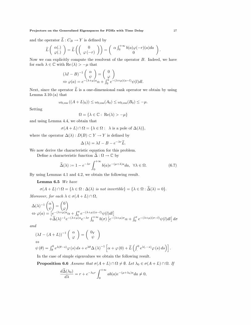
and the operator L : CB → Y is defined by

L

(α(.)ϕ(.)

)= L

((0

ϕ (−r)

))=

(α

∫ +∞0

b(a)ϕ(−r)(a)da0

).

Now we can explicitly compute the resolvent of the operator B. Indeed, we havefor each λ ∈ C with Re (λ) > −µ that

(λI −B)−1

(αψ

)=

(0ϕ

)

⇔ ϕ(a) = e−(λ+µ)aα +∫ a

0e−(λ+µ)(a−l)ψ(l)dl.

Next, since the operator L is a one-dimensional rank operator we obtain by usingLemma 3.10-(a) that

ω0,ess ((A + L)0)) ≤ ω0,ess(A0) ≤ ω0,ess(B0) ≤ −µ.

SettingΩ = λ ∈ C : Re(λ) > −µ

and using Lemma 4.4, we obtain that

σ(A + L) ∩ Ω = λ ∈ Ω : λ is a pole of ∆(λ),where the operator ∆(λ) : D(B) ⊂ Y → Y is defined by

∆ (λ) = λI −B − e−λrL.

We now derive the characteristic equation for this problem.Define a characteristic function ∆ : Ω → C by

∆(λ) := 1− e−λr

∫ +∞

0

b(a)e−(µ+λ)ada, ∀λ ∈ Ω. (6.7)

By using Lemmas 4.1 and 4.2, we obtain the following result.

Lemma 6.5 We have

σ(A + L) ∩ Ω = λ ∈ Ω : ∆(λ) is not invertible = λ ∈ Ω : ∆(λ) = 0.Moreover, for each λ ∈ σ(A + L) ∩ Ω,

∆(λ)−1

(αψ

)=

(0ϕ

)

⇔ ϕ(a) =[e−(λ+µ)aα +

∫ a

0e−(λ+µ)(a−l)ψ(l)dl

]

+∆(λ)−1e−(λ+µ)ae−λr∫ +∞0

b(σ)[e−(λ+µ)σα +

∫ σ

0e−(λ+µ)(σ−l)ψ(l)dl

]dσ

and

(λI − (A + L))−1

(αϕ

)=

(0Y

ψ

)

⇔ψ (θ) =

∫ 0

θeλ(θ−s)ϕ (s) ds + eλθ∆ (λ)−1

[α + ϕ (0) + L

(∫ 0


)].

In the case of simple eigenvalues we obtain the following result.

Proposition 6.6 Assume that σ(A + L) ∩ Ω 6= ∅. Let λ0 ∈ σ(A + L) ∩ Ω. If

d∆(λ0)dλ

= r + e−λ0r

∫ +∞

0

ab(a)e−(µ+λ0)ada 6= 0,


then λ0 is a pole of order 1 of (λI − (A + L))−1 and

Bλ−1

(αϕ

)=

(0

eλθ∆−1

[α + ϕ (0) + L

(∫ 0


)])

,

where the linear operator ∆−1 = limλ→λ0 (λ− λ0)∆ (λ)−1 is defined by

∆−1

(αψ

)=

(0ϕ

)

⇔ ϕ(a) = d∆(λ0)dλ

−1

e−(λ0+µ)ae−λ0r∫ +∞0

b(σ)[e−(λ0+µ)σα +

∫ σ

0e−(λ0+µ)(σ−l)ψ(l)dl

]dσ.

References

[1] M. Adimy, Bifurcation de Hopf locale par des semi-groupes integres, C. R. Acad. Sci. ParisSerie I 311 (1990), 423-428.

[2] M. Adimy, Integrated semigroups and delay differential equations, J. Math. Anal. Appl. 177(1993), 125-134.

[3] M. Adimy and O. Arino, Bifurcation de Hopf globale pour des equations a retard par dessemi-groupes integres, C. R. Acad. Sci. Paris Serie I 317 (1993), 767-772.

[4] M. Adimy, K. Ezzinbi and J. Wu, Center manifold and stability in critical cases for somepartial functional differential equations, Int. J. Evol. Equ. 2 (2007), 47–73.

[5] W. Arendt, Vector valued Laplace transforms and Cauchy problems, Israel J. Math. 59(1987), 327-352.

[6] W. Arendt, C. J. K. Batty, M. Hieber, and F. Neubrander, Vector-Valued Laplace Transformsand Cauchy Problems, Birkhauser, Basel, 2001.

[7] O. Arino, M. L. Hbid and E. Ait Dads, Delay Differential Equations and Applications,Springer, Berlin, 2006.

[8] O. Arino and E. Sanchez, A variation of constants formula for an abstract functional-differential equation of retarded type, Differential Integral Equations 9 (1996), 1305–1320.

[9] O. Arino and E. Sanchez, A theory of linear delay differential equations in infinite dimen-sional spaces, in “Delay Differential Equations with Application”, O. Arino, M. Hbid andE. Ait Dads (eds.), NATO Science Series II: Mathematics, Physics and Chemistry, Vol. 205,Springer, Berlin, 2006, pp. 287-348.

[10] H. Brezis, Analyse Fonctionnelle, Dunod, Paris, 2005[11] F. E. Browder, On the spectral theory of elliptic differential operators, Math. Ann. 142

(1961), 22-130.[12] S. Busenberg and W. Huang, Stability and Hopf bifurcation for a population delay model

with diffusion effects, J. Differential Equations 124 (1996), 80-107.[13] O. Diekmann, P. Getto and M. Gyllenberg, Stability and bifurcation analysis of Volterra

functional equations in the light of suns and stars, SIAM J. Math. Anal. 34 (2007), 1023-1069.

[14] O. Diekmann, S. A. van Gils, S. M. Verduyn Lunel, and H.-O. Walther, Delay Equations,Function-, Complex-, and Nonlinear Analyiss, Springer-Verlag, New York, 1995.

[15] A. Ducrot, Z. Liu and P. Magal, Essential growth rate for bounded linear perturbation ofnon-densely defined Cauchy problems, J. Math. Anal. Appl. 341 (2008), 501–518.

[16] K.-J. Engel and R. Nagel, One Parameter Semigroups for Linear Evolution Equations,Springer-Verlag, New York, 2000.

[17] K. Ezzinbi and M. Adimy, The basic theory of abstract semilinear functional differentialequations with non-dense domain, in “Delay Differential Equations with Application”, O.Arino, M. Hbid and E. Ait Dads (eds.), NATO Science Series II: Mathematics, Physics andChemistry, Vol. 205, Springer, Berlin, 2006, pp. 349-400.

[18] T. Faria, Normal forms and Hopf bifurcation for partial differential equations with delays,Trans. Amer. Math. Soc. 352 (2000), 2217-2238.

[19] T. Faria, W. Huang and J. Wu, Smoothness of center manifolds for maps and formal adjointsfor semilinear FDEs in general Banach spaces, SIAM J. Math. Anal. 34 (2002), 173–203.

[20] W. E. Fitzgibbon, Semilinear functional differential equations in Banach space, J. DifferentialEquations 29 (1978), 1–14.


[21] M. V. S. Frasson and S. M. Verduyn Lunel, Large time behaviour of linear functional differ-ential equations, Integr. Equ. Oper. Theory 47 (2003), 91-121.

[22] J. K. Hale and S. M. Verduyn Lunel, Introduction to Functional Differential Equations,Springer-Verlag, New York, 1993.

[23] B. D. Hassard, N. D. Kazarinoff and Y.-H. Wan, Theory and Applications of Hopf Bifurcaton,Londonn Math. Soc. Lect. Note Ser. 41, Cambridge Univ. Press, Cambridge, 1981.

[24] M. A. Kaashoek and S. M. Verduyn Lunel, Characteristic matrices and spectral propertiesof evolutionary systems, Trans. Amer. Math. Soc. 334 (1992), 479-517.

[25] F. Kappel, Linear autonomous functional differential equations, in “Delay Differential Equa-tions with Application”, O. Arino, M. Hbid and E. Ait Dads (eds.), NATO Science Series II:Mathematics, Physics and Chemistry, Vol. 205, Springer, Berlin, 2006, pp. 41-134.

[26] H. Kellermann and M. Hieber, Integrated semigroups, J. Funct. Anal. 84 (1989), 160-180.[27] X. Lin, J. W.-H. So and J. Wu, Centre manifolds for partial differential equations with delays,

Proc. Roy. Soc. Edinburgh 122A (1992), 237-254.[28] Z. Liu, P. Magal and S. Ruan, Projectors on the generalized eigenspaces for functional differ-

ential equations using integrated semigroups, J. Differential Equations 244 (2008), 1784-1809.[29] Z. Liu, P. Magal, S. Ruan and J. Wu, Normal forms for semilinear equations with non-dense

domain, Part I: Computation of the reduced system, submitted.[30] R. H. Martin and H. L. Smith, Abstract functional-differential equations and reaction-

diffusion systems, Trans. Amer. Math. Soc. 321 (1990), 1–44.[31] R. H. Martin and H. L. Smith, Reaction-diffusion systems with time delays: monotonicity,

invariance, comparison and convergence, J. Reine Angew. Math. 413 (1991), 1–35.[32] P. Magal, Compact attractors for time periodic age-structured population models, Electr. J.

Differential Equations 2001 (2001), No. 65, 1-35.[33] P. Magal and S. Ruan, On integrated semigroups and age structured models in Lp spaces,

Differential Integral Equations 20 (2007), 197-239.[34] P. Magal and S. Ruan, On semilinear Cauchy problems with non-dense domain, Adv. Dif-

ferential Equations 14 (2009), 1041-1084.[35] P. Magal and S. Ruan, Center manifold theorem for semilinear equations with non-dense

domain and applications to Hopf bifurcations in age structured models, Mem. Amer. Math.Soc. Vol. 202, 2009, No. 951.

[36] M. C. Memory, Bifurcation and asymptotic behavior of solutions of a delay-differential equa-tion with diffusion, SIAM J. Math. Anal. 20 (1989), 533–546.

[37] M. C. Memory, Stable ans unstable manifolds for partial functional differential equations,Nonlinear Anal. 16 (1991), 131-142.

[38] M. E. Parrott, Linearized stability and irreducibility for a functional-differential equation,SIAM J. Math. Anal. 23 (1992), 649–661.

[39] A. Pazy, Semigroups of Linear Operators and Applications to Partial Differential Equations,Springer-Verlag, New-York, 1983.

[40] A. Rhandi, Extrapolated methods to solve non-autonomous retarded partial dierential equa-tions, Studia Math. 126 (1997), 219-233.

[41] S. Ruan, J. Wei and J. Wu, Bifurcation from a homoclinic orbit in partial functional differ-ential equations, Discret. Contin. Dynam. Syst. 9A (2003), 1293-1322.

[42] S. Ruan and W. Zhang, Exponential dichotomies, the Fredholm alternative, and transversehomoclinic orbits in partial functional differential equations, J. Dynamics Differential Equa-tions 17 (2005), 759-777.

[43] W. M. Ruess, Existence and stability of solutions to partial functional differential equationswith delay, Adv. Differential Equations 4 (1999), 843-867.

[44] W. M. Ruess, Linearized stability for nonlinear evolution equations, J. Evol. Equ. 3 (2003),361-373.

[45] H. R. Thieme, Semiflows generated by Lipschitz perturbations of non-densely defined opera-tors, Differential Integral Equations 3 (1990), 1035-1066.

[46] H. R. Thieme, Integrated semigroups and integrated solutions to abstract Cauchy problems,J. Math. Anal. Appl. 152 (1990), 416-447.

[47] H. R. Thieme, Quasi-compact semigroups via bounded perturbation, in “Advances in Math-ematical Population Dynamics—Molecules, Cells and Man”, Ser. Math. Biol. Med. Vol. 6,World Sci. Publishing, River Edge, NJ, 1997, pp. 691-711.


[48] C. C. Travis and G. F. Webb, Existence and stability for partial functional differential equa-tions, Trans. Amer. Math. Soc. 200 (1974), 395-418.

[49] C. C. Travis and G. F. Webb, Existence, stability, and compactness in the α-norm for partialfunctional differential equations, Trans. Amer. Math. Soc. 240 (1978), 129-143.

[50] S. M. Verduyn Lunel, Spectral theory for delay equations, in “Systems, Approximation, Sin-gular Integral Operators, and Related Topics”, A. A. Borichev and N. K. Nikolski (eds.),Operator Theory: Advances and Applications, Vol. 129, Birkhauser, 2001, pp. 465-508.

[51] G. F. Webb, Functional differential equations and nonlinear semigroups in Lp-spaces, J.Differential Equations 20 (1976), 71-89.

[52] G. F. Webb, Theory of Nonlinear Age-Dependent Population Dynamics, Marcel Dekker, NewYork, 1985.

[53] G. F. Webb, An operator-theoretic formulation of asynchronous exponential growth, Trans.Amer. Math. Soc. 303 (1987), 155-164.

[54] J. Wu, Theory and Applications of Partial Differential Equations, Springer-Verlag, New York,1996.

[55] K. Yoshida, The Hopf bifurcation and its stability for semilinear diffusion equations withtime delay arising in ecology, Horoshima Math. J. 12 (1982), 321-348.

Projectors on the Generalized Eigenspaces for Partial...

Documents

Transcript of Projectors on the Generalized Eigenspaces for Partial...