Projective Compactification of R1,1 and its Mobius

Geometry

John A. Emanuello and Craig A. Nolder

February 1, 2014

Abstract

We examine the semi-Riemannian manifold R1,1, which is realized as the split complexplane, and its conformal compactifcation as an analogue of the complex plane and the Riemannsphere. We also consider conformal maps on the compactifcation and study some of their basicproperties.

1 Introduction

There are many advantages of using the Riemann sphere instead of the complex plane as a domainfor functions of a complex variable. As a compact space, it possesses some desirable topologicalproperties. In terms of the analysis, one finds that many nice results are true on the sphere whichare not true in the plane. For example the class of meromorphoric functions on the sphere aremerely the rational functions, while in the plane the meormorphic functions are a larger class offunctions. Also, the sphere has a rich conformal geometry.

In this work, we consider the split complex numbers R1,1, which is just the semi-Riemannianmanifold R2 with the semi-Riemannian (or indefinite) metric

g (X,Y ) = X1Y1 −X2Y2.

We put an algebraic structure on R1,1 by identifying it with the Clifford algebra C`1,0. With thisadditional structure, we are able to define differential operators and develop a holomorphic functiontheory parallel to that of the complex plane. A natural question rises: Can we find a better domainfor functions of a split complex variable, like we do in complex analysis?

This is a question which has been addressed over many years and in many places in the literature,although not always directly, but always in the affirmative [1–3]. M. Schottenloher linked theprevious question with questions of conformality [4]. In particular, Schottenloher describes a modelfor compactifying Rp,q with an induced conformal structure, building on the work of Dirac, whoused an analogous model for the compactification of four-dimensional spacetime several decadesearlier.

1

Schottenloher also discusses the notion of conformal group on R1,1 and identifies it as a productof circle diffeomorphisms. It is not clear if the work extends these to the compactification. Theauthors have been unable to find a work which clearly identifies the collection of linear fractionaltransformations as a subgroup of the conformal group, even though this is the case. This work doesmake this clear and develops a Mobius transformation theory for R1,1.

Yaglom also defined a cross ratio on R1,1 in [2], which seems to have been largely overlooked orforgotten until [5]. This cross ratio has been previously shown to be well behaved with respect tothe Mobius transformations, but this also seems to have been lost.

The purpose of this work is threefold. First, we wish to carefully construct the compactificationof R1,1 in a conformal setting. Second, we use holomorphic and conformal conditions in R1,1 toextend these notions to the compactification in a simple way. Last, we use algebraic properties ofthe split complex numbers to show that the Mobius transformations are a direct product of realMobius transformations and to discuss their conformality, transitivity, and fixed points carefully(something which has not been found in a rather thorough review of the literature).

Our paper is organized as follows. In Section 2, we give a quick overview of the split complexnumbers and the analysis of functions of a split complex variable. We also introduce a notion ofconformal mappings over R1,1 and briefly describe some involutions of the torus in R4. ThroughoutSection 3, we examine the compactification in some detail, which we denote Q1,1, and its geometricproperties. We also extend the definition of differentiablity to Q1,1, and provide simple criteria fordetermining conformality. Last, Section 4 serves as an examination of Mobius transformations andtheir fixed points and transitivity. We also study the cross ratio and show that hyperbolae play asimilar role here that circles do in complex analysis.

2 Preliminaries

2.1 Split Complex Numbers R1,1

The algebra of split complex numbers, or double numbers (as in [6]),

R1,1 =ζ = x+ yj | x, y ∈ R, j2 = 1

,

is the Clifford algebra C`1,0 generated as an algebra over R by 1 and j. Even though R1,1 resemblesC, it has a different algebraic structure. In particular, R1,1 has zero divisors:

(1 + j)(1− j) = 1− j2 = 0.

However, if we define

j+ =(1 + j)

2and j− =

(1− j)2

,

we get a useful basis for R1,1:ζ = uj+ + vj−,

2

where u = x+ y, v = x− y. Notice that j+ and j− square to themselves and annihilate each other.Thus, multiplication simplifies in these new coordinates:

(u1j+ + v1j−)(u2j+ + v2j−) = u1u2(j+)2 + u1v2j+j− + v1u2j−j+ + v1v2(j−)2

= u1u2j+ + v1v2j−.

This means R1,1 is isomorphic as an algebra to R⊕ R, which is also is the space of 2× 2 diagonalmatrices with real entries [7].

It is now clear that the zero divisors in C`1,0 are precisely those elements which can be written

ζ = αj+ or ζ = αj−,

for α ∈ R. These elements are called the light cone and we denote it by L. Clearly, L is the unionof two one-dimensional subspaces,

L+ = αj+ : α ∈ R and L− = αj− : α ∈ R .

When defined, the inverse is given by

ζ−1 = u−1j+ + v−1j−.

It is also be useful to invert only one of the components:

ζ−1+ = u−1j+ + vj− and

ζ−1− = uj+ + v−1j−.

We define a conjugation operation for the split complex numbers which resembles what we havein C:

C(ζ) = ζ = x− jy = vj+ + uj−.

Unlike in C, however, the map

N(ζ) = ζζ

= x2 − y2

= uv.

does not induce a norm in C`1,0, since the positivity condition fails. However, N(ζ) is a pseudo-norm.

Remark 2.1. The element ζ ∈ C`1,0 is also in L if and only if N(ζ) = 0.

2.2 Analysis of Functions of a Split-Complex Variable

Now, we consider functions of a split complex variable:

f : U ⊆ R1,1 → R1,1.

3

Such functions have been examined in numerous places [6, 8, 9]. Here U is an open subset of R1,1.

These functions may be written f(z) = f1(x, y) + jf2(x, y). Throughout this work, we shallassume that f1, f2 ∈ C1 (U). Now just as in complex analysis, we must understand what it meansfor the limit of the difference quotient

limh→0h/∈L

f(z0 + h)− f(z0)h

to exist.

Now suppose this limit exists and assume that h = hx is real. Then

limhx→0

f(z0 + hx)− f(z0)hx

= limhx→0

f1(x0 + hx, y0)− f1(x0, y0)hx

+ jf2(x0 + hx, y0)− f2(x0, y0)

hx

=∂f1∂x

(x0, y0) + j∂f2∂x

(x0, y0).

Similarly, if we assume h = jhy is purely imaginary then

limjhy→0

f(z0 + jhy)− f(z0)jhy

= j∂f1∂y

(x0, y0) +∂f2∂x

(x0, y0).

Remark 2.2. This gives the Cauchy-Riemann equations in the split complex plane [8]:

∂f1∂x

=∂f2∂y

and∂f1∂y

=∂f2∂x

.

Conversely, if these equations are satisfied and the partial derivatives are continuous, then thelimit of the difference quotient exists (just as in complex analysis). If either of these conditions aresatisfied, then we say that f is C`0,1-differentiable at z0. If this is the case for all z0 ∈ U we say fis C`0,1-differentiable on U .

Now consider the differential operator

∇ =12

(∂

∂x− j ∂

∂y

)and its conjugate

∇ =12

(∂

∂x+ j

∂

∂y

)which clearly satisfies

∇∇ = ∇∇ =14

(∂2

∂x2− ∂2

∂y2

),

which is the wave operator in the plane. Functions which are annihilated by the wave operator arecalled hyperharmonic.

4

Remark 2.3. This means that the components of a C`0,1-differentiable function satisfy the waveequation in the plane [9]. Complex holomorphic functions have components which satisfy Laplace’sequation [10].

Theorem 2.4. Let f be a split complex valued function of a split complex variable.

∇f(z0) = 0 ⇐⇒ f is C`0,1-differentiable at z0.

Proof. Notice that

∇(f1 + jf2) =12

[∂f1∂x

+ j∂f2∂x− j ∂f1

∂y− ∂f2

∂y

]=

12

[(∂f1∂x− ∂f2

∂y

)+ j

(∂f2∂x− ∂f1

∂y

)].

Thus ∇(f1 + jf2) = 0 if and only if f is C`0,1-differentiable.

Definition 2.5. We say a split complex valued function of a split complex variable f is C`0,1-antidifferentiable at z0 if

∇f(z0) = 0

Corollary 2.6. Given a hyperharmonic function g : U ⊆ R2 → R, the function f = ∇g is C`0,1-differentiable and h = ∇g is C`0,1-antidifferentiable.

If we use our alternative basis for split complex plane, we may rewrite

∇ =12

(∂

∂x− j ∂

∂y

)=

12

[(∂u

∂x

∂

∂u+∂v

∂x

∂

∂v

)− j

(∂u

∂y

∂

∂u+∂v

∂y

∂

∂v

)]=

12

[∂

∂u+

∂

∂v− j ∂

∂u+ j

∂

∂v

]=

∂

∂vj+ +

∂

∂uj−.

It is easy to see that

∇ =∂

∂uj+ +

∂

∂vj−,

so that

∇∇ = ∇∇ =∂2

∂u∂v,

for reasonably behaved f(u, v).

This gives us the following corollary [9].

5

Corollary 2.7. The split complex valued function f is C`0,1-differentiable if and only if

f = f1(u)j+ + f2(v)j−.

Also, f is C`0,1-antidifferentiable if and only if

f = f1(v)j+ + f2(u)j−.

With this new method for checking differentiability, we are able to check that analogues of someholomorphic functions in C are C`0,1-differentiable in R1,1.

Example 2.8. Let f(ζ) = ζm for a positive integer m. Then f is C`0,1-differentiable, and henceso are split-complex polynomials.

Proof. With the simplified multiplication in the coordinates ζ = uj+ + vj−, we have that

ζm = umj+ + vmj−.

It will be useful to have a notion of meromorphic functions.

Definition 2.9. Let f be a split complex valued function of a split complex variable. We say f isC`0,1-meromorphic if

f = f1(u)j+ + f2(v)j−,

and f1, f2 are real meromorphic functions. We say f is C`0,1-antimeromorphic if

f = f1(v)j+ + f2(u)j−,

and f1, f2 are real meromorphic functions.

2.3 Analogues of Complex Analysis

The notion of C`0,1-differentiablity yields some analogues of theorems from complex analysis. Inparticular, we have an analogue of Cauchy’s Theorem.

Proposition 2.10. Let U ⊆ C`1,0 be open (in the Euclidean topology of R2). Suppose S ⊆ U isbounded, orientable subdomain with a piecewise differentiable boundary. If f is C`1,0-differentiableon U , then ∫

∂S

fdz = 0,

where dz = dx+ jdy

The proof, which can be found in [9], uses Stoke’s Theorem.

There is also an analogue of the Cauchy Integral formula, which is presented in [9]. However,we find that because C`1,0 is not a field, we do not use a C`1,0-valued kernel. Rather, we will usea kernel which takes values in C`1,0 ⊗ C.

6

Lemma 2.11. Define K : (C`1,0)× → (C`1,0)× by

K(z) = z−1 =z

N(z).

Then ∇K(z) = 0 for every z ∈ (C`1,0)×.

To obtain the kernel we seek, we simply “complexify” K. Define

Kε(x+ jy) =1 + j

2· 1x+ y + iε · sign(x− y)

+1− j

2· 1x− y + iε · sign(x+ y)

.

Proposition 2.12 (Libine’s Integral Formula). Let R > 0 and define S = z ∈ C`1,0 : |N(z)| < R.Let U be an open neighborhood of S. Suppose f : U → C`1,0 is smooth and ∇f = 0. Then for anyζ ∈ S,

f(ζ) =1

2πilimε→0

∫|N(z)|=R

Kε(z − ζ)f(z)dz.

The proof is found in [9].

2.4 Conformal Mappings of R1,1

Recall that R1,1 is a semi-Riemannian manifold with indefinite metric g1,1 of signature (1, 1):

g1,1(X,Y ) = X1Y1 −X2Y2.

In the literature, a smooth map f : U ⊂ X → X on a semi-Riemannian manifold (X, g) ofmaximal rank (that is, f is a local diffeomorphism) is called (locally) conformal on U if there is asmooth map Ω : U → R>0 such that

f∗g = Ωg,

where f∗g(X,Y ) = g(df(X), df(Y ), and df is the tangent map of f [4].

However, we will opt for a global definition of conformal mappings on R1,1. Indeed, we shallrequire such maps to be globally one-to-one. Also, we will not require C∞ smoothness; rather, C1

smooth will be enough. Given that we are using an indefinite metric, we find the condition that Ωbe positive to be too restrictive. Moreover, we will only require Ω to be non-zero.

For R1,1, Schottenloher shows that the conformal factor has a simple form [4]:

Ω =(∂f1∂x

)2

−(∂f2∂x

)2

=(∂f2∂y

)2

−(∂f1∂y

)2

.

Moreover, we get a simple condition to check for conformality.

Theorem 2.13. A one-to-one C1 map f : R1,1 → R1,1, where f = f1(x, y) + jf2(x, y), is (locally)conformal when either

7

1. ∇f = 0 and(∂f1∂x

)2

−(∂f2∂x

)2

6= 0, or

2. ∇f = 0 and(∂f1∂x

)2

−(∂f2∂x

)2

6= 0,

everywhere on R1,1.

If we use the alternative basis, these conditions are

1. ∇f = 0 and(∂g1∂u

)(∂g2∂v

)6= 0, or

2. ∇f = 0 and(∂g1∂v

)(∂g2∂u

)6= 0,

where f = g1(u, v)j+ + g2(u, v)j−.

Proof. The proof in the original basis for positive conformal factor can be found in [4]. Requiringa non-vanishing conformal factor does not change the proof. Thus, it only remains to show thatthe first set of conditions (that is those in the original basis) are equivalent to the second set ofconditions.

Suppose ∇f = 0. Thus,

f(ζ) = f1(x, y) + f2(x, y)j = g1(u)j+ + g2(v)j−,

so that

f1 =g1(u) + g2(v)

2and f2 =

g1(u)− g2(v)2

.

Recall,∂

∂x=

∂

∂u+

∂

∂v.

Then,

∂f1∂x

=12

[∂

∂u(g1(u) + g2(v)) +

∂

∂v(g1(u)− g2(v))

]=

12

[∂g1∂u

+∂g2∂v

].

Similarly,∂f2∂x

=12

[∂g1∂u− ∂g2

∂v

].

Thus, (∂f1∂x

)2

−(∂f2∂x

)2

=(∂g1∂u

)(∂g2∂v

).

8

That is, the first conditions in each set are equivalent. A similar argument shows the equivalenceof the second ones.

Soon, we will see that Mobius transformations of R1,1 are a large, but not exhaustive class ofconformal mappings.

2.5 The Torus in R4

Our study of the torus is motivated by our desire to find a compactification of R1,1. That is, we arelooking for a space where we can embed R1,1 and the analysis, topology, and geometry are analogousto the Riemann sphere. The torus does not provide the model we need for the compactifcation, butit is close to what we need.

We denote the torus S1 × S1 embedded in R4 as follows:

T 1,1 = (x0, x1, x2, x3)|x20 + x2

1 = 1, x22 + x2

3 = 1.

The torus T 1,1 is the union of two disjoint open sets along with their common boundary:

T 1,1 = T 1,1+ ∪ T 1,1

− ∪ T1,10

where T 1,1+ = x ∈ T 1,1|x0 +x3 > 0, T 1,1

− = x ∈ T 1,1|x0 +x3 < 0 and T 1,10 = x ∈ T 1,1|x0 +x3 =

0.

We define some involutions of T 1,1 which are also bijective diffeomorphisms. They will also playan important role in developing the compactification of R1,1.

Definition 2.14. a. We define some involutions of T 1,1 :

i. Left Inversion: J+(x) = (x2, x3, x0, x1);

ii. Right Inversion: J−(x) = (−x2, x3,−x0, x1);

iii. Inversion: J(x) = (−x0, x1,−x2, x3) = J+(x) J−(x).

b. The following involutions preserve T 1,10 :

iv. Left Negation: N+(x) = (x3,−x2,−x1, x0);

v. Right Negation: N−(x) = (x3, x2, x1, x0);

vi. Negation: N(x) = (x0,−x1,−x2, x3) = N+(x) N−(x);

vii. Conjugation: C(x) = (x0, x1,−x2, x3);

viii. Reflection: R(x) = (−x0,−x1,−x2,−x3) = J+ N J+ N(x).

9

3 The Conformal Compactification of R1,1

The notion of compactifying R1,1 is well known (see [3,11]) and is of some interest to physicists [4,12,13]. One finds that this problem has been explained in numerous places in the literature, thoughthere are some differences in the models used. For example, Kisil and others use a hyperboloidmodel in extended 3-space [6, 14], and in others as a quadric in projective space [4]. In this work,we utilize the quadric model, which we denote Q1,1. However, we follow the largely forgottenmethod presented in Segal’s book (see [3]): we construct the compactification by way of torus onwhich we embed R1,1 and then quotient by a projection.

We shall define the conformal compactification of R1,1 as follows.

Definition 3.1. A conformal compactification, up to isomorphism, of R1,1 is a compact semi-Riemannian manifold M with a conformal embedding ι such that ι(R1,1) is dense in M .

Remark 3.2. In this context, the sphere S2 is the conformal compactification of C with the stere-ographic projection as a conformal embedding.

3.1 Embedding of R1,1 onto Q1,1

A preliminary step to constructing the conformal compactification is to find a way to embed R1,1

in the torus. This embedding τ : R1,1 → T 1,1+ is given by

τ(ζ) = τ(u, v) =(1− uv, u+ v, u− v, 1 + uv)√

(1 + u2)(1 + v2),

and is a bijective diffeomorphism of R1,1 onto T 1,1+ . Later, we shall see that τ is a conformal mapping

with respect to the semi-Riemannian metric on R1,1 and Q1,1. We remark the R(τ(ζ)) is a bijectivediffeomorphism of R1,1 onto T 1,1

− .

Notice that for ζ ∈ R1,1, when the inverses exist,

τ(ζ) = C(τ(ζ)),

τ(ζ−1) = ±J(τ(ζ)),

τ(ζ−1+ ) = ±J+(τ(ζ)),

τ(ζ−1− ) = ±J−(τ(ζ)).

Similar formulas hold for N,N+, N−:

τ(−ζ) = N(τ(ζ)),τ(−uj+ + vj−) = N+(τ(ζ)),τ(uj+ − vj−) = N−(τ(ζ)).

Also notice that J+ and N do not commute on T 1,1 :

N J+(x) = (x2,−x3,−x0, x1) 6= J+ N(x) = (−x2, x3, x0,−x1),

10

even though the corresponding involutions on R1,1 commute. As such we descend to the projectivespace of the torus, which turns out to be the conformal compactification we seek (and we shall seewhy this is true in the subsequent subsections).

Definition 3.3. We define a quadric surface Q1,1 in the projective space P3 by

Q1,1 = T 1,1/ ∼

under the equivalence

x ∼ y if and only if x = ±y.

Remark 3.4. We denote this identification by π.

Notice that this equivalence identifies x and R(x) and hence points in T 1,1+ with points in T 1,1

−and points in T 1,1

0 with points in T 1,10 . These identified points are pairs of antipodal points on the

3-sphere containing T 1,1.

We denote points in Q1,1 by (x0 : x1 : x2 : x3). As a matter of notation, if (x0 : x1 : x2 : x3) ∈Q1,1, then we assume that (λx0 : λx1 : λx2 : λx3) represents this point for all non-zero λ ∈ R.

The inverse mapping τ−1 : T 1,1+ → R1,1 is given by

u =x1 + x2

x0 + x3,

v =x1 − x2

x0 + x3.

Notice that τ−1 extends to T 1,1+ ∪ T 1,1

− as a two to one cover of R1,1.

For notational convenience, we shall denote the composition π τ by

η : R1,1 → Q1,1.

We shall also extend our definition of inversion to Q1,1:

(x0 : x1 : x2 : x3) 7→ (−x0 : x1 : −x2 : x3).

For simplicity we shall also denote this J (there should be no ambiguity sinceπ J τ = J η.)

3.2 Added Points

The conformal compactification of C has one more point than the plane, namely the point at infinity.For R1,1, we must add an additional point for every point in the light cone plus two additional pointswhich compactify the light cone. We calculate the coordinates of these additional points.

11

Suppose v = 0. Thenη(ζ) = (1 : u : u : 1),

which goes to (0 : 1 : 1 : 0) as u→∞, and

Jη(ζ) = (−1 : u : −u : 1),

goes to (0 : 1 : −1 : 0) as u→∞. When u = 0,

η(ζ) = (1 : v : −v : 1),

goes to (0 : 1 : −1 : 0) as v →∞, and

Jη(ζ) = (−1 : v : v : 1),

tends to (0 : 1 : 1 : 0) as v →∞.

Throughout −∞ < α <∞, define

L+ = η(L+) = (1 : α : α : 1) and L− = η(L−) = (1 : α : −α : 1).

The above observations give us the following.

Remark 3.5. If we define

L−1+ := Jη(L+) = (−1 : α : −α : 1) : α ∈ R ∪ (0 : 1 : −1 : 0) and

L−1− := Jη(L−) = (−1 : α : α : 1) : α ∈ R ∪ (0 : 1 : 1 : 0).

Then these intersect at πJ(τ(0)) = (−1 : 0 : 0 : 1) and we shall define Q1,10 := L−1

+ ∪ L−1− .

Remark 3.6. To avoid an unnecessarily cumbersome notation, we shall adopt the following:

1. 1αj+ +∞j− shall denote (−1 : α : −α : 1).

2. ∞j+ + 1αj− shall denote (−1 : α : α : 1).

3. ∞j+ shall denote (0 : 1 : 1 : 0).

4. ∞j− shall denote (0 : 1 : −1 : 0).

5. ∞ shall denote ∞j+ +∞j− = 10 , the inversion of zero.

In this manner, it is clear that elements of Q1,1 can be regarded as elements R × R, where R :=R ∪ ∞. In fact, Q1,1 is locally isomorphic to R × R (in the sense of conformal geometry) [4].These are sometimes referred to as the “extended double numbers” [6].

Other rays through the origin embed as follows. If u = βv, β 6= 0, then

η(ζ) = (1− βu2 : (1 + β)u : (1− β)u : 1 + βu2),

12

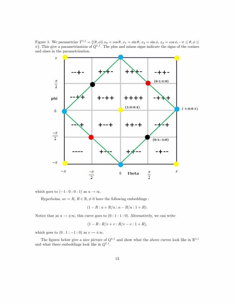
Figure 1: We parametrize T 1,1 = (θ, φ)|x0 = cos θ, x1 = sin θ, x2 = sinφ, x3 = cosφ,−π ≤ θ, φ ≤π. This give a parametrization of Q1,1. The plus and minus signs indicate the signs of the cosinesand sines in the parametrization.

which goes to (−1 : 0 : 0 : 1) as u→∞.

Hyperbolas, uv = R, R ∈ R, 6= 0 have the following embeddings :

(1−R : u+R/u : u−R/u : 1 +R).

Notice that as u→ ±∞, this curve goes to (0 : 1 : 1 : 0). Alternatively, we can write

(1−R : R/v + v : R/v − v : 1 +R),

which goes to (0 : 1 : −1 : 0) as v → ±∞.

The figures below give a nice picture of Q1,1 and show what the above curves look like in R1,1

and what there embeddings look like in Q1,1.

13

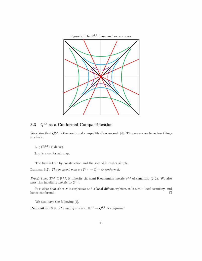
Figure 2: The R1,1 plane and some curves.

3.3 Q1,1 as a Conformal Compactification

We claim that Q1,1 is the conformal compactifcation we seek [4]. This means we have two thingsto check:

1. η(R1,1

)is dense;

2. η is a conformal map.

The first is true by construction and the second is rather simple:

Lemma 3.7. The quotient map π : T 1,1 → Q1,1 is conformal.

Proof. Since T 1,1 ⊆ R2,2, it inherits the semi-Riemannian metric g2,2 of signature (2, 2). We alsopass this indefinite metric to Q1,1.

It is clear that since π is surjective and a local diffeomorphism, it is also a local isometry, andhence conformal.

We also have the following [4].

Proposition 3.8. The map η = π τ : R1,1 → Q1,1 is conformal.

14

Figure 3: The embedded curves. Points with the same numeric label are identified.

Remark 3.9. Under certain conditions we can take a conformal map

f : R1,1 → R1,1

and extend it to a conformal mapf : Q1,1 → Q1,1.

In particular, when ζ, f(ζ) ∈ η(R1,1

), f(ζ) = η f η−1. In such a case we continue to write

f(ζ) for f(1− uv : u+ v : u− v : 1 + uv).

At Q1,10 , f is continuous, and this means that the values of such points can be defined as limits.

For example,f(0 : 1 : 1 : 0) = lim

u→∞f(1 : u : u : 1).

3.4 Differentiable Functions and Conformal Mappings on Q1,1

We want to define a notion of differentiability on Q1,1 which is consistent the notion of differentia-bility on R1,1 defined in Section 2.2. This has been explored on the equivalent space of extendeddouble numbers in [6]. We shall proceed in a similar fashion and borrow some ideas from complexanalysis (as in [10]). In complex analysis one adds a point at infinity to invert the origin anddiscusses the behavior of functions at this added point using the inversion. In a similar way, weinvert the added points to investigate functions at these added points. We define the following setsand maps for this purpose. They do not serve as an atlas.

15

A1 = η(R1,1

), φ1 = η−1

A2 = ∞ , φ2 = η−1 JA3 = L−1

+ \ ∞ , φ3 = η−1 J+

A4 = L−1− \ ∞ , φ4 = η−1 J−

Definition 3.10. Consider the function

f : Q1,1 → Q1,1,

and ζ0 ∈ Q1,1. Suppose ζ0 ∈ Ai and f(ζ0) ∈ Aj. We say f is Q1,1-differentiable at ζ0 if

φj f φ−1i

is C`1,0-differentiable at η−1(ζ0). If f is Q1,1-differentiable everywhere, we will say f is Q1,1-differentiable.

We also define Q1,1-meromorphic (and Q1,1-antimeromorphic) as functions of the form f1(u)j++f2(v)j− (resp. f1(v)j+ + f2(u)j−), where f1 and f2 are meromorphic functions on R.

We recall that Q1,1 inherits the semi-Riemannian metric g2,2. Hence, a notion of conformal mapis defined. By using the conformality of η, J , and J± on their respective domains to get a shortcutdefinition for conformality of maps f : Q1,1 → Q1,1, :

Theorem 3.11. A functionf : Q1,1 → Q1,1

is (globally) conformal iff the mapsφj f φ−1

i

are conformal (in the sense of Theorem 2.13 ) everywhere they are defined.

First we need some lemmas:

Lemma 3.12. The maps J, J+, J− : Q1,1 → Q1,1 are conformal.

Proof. Write p = (x0 : x1 : x2 : x3). Then J(p) = (−x0 : x1 : −x2 : x3), and

dJ =

−1 0 0 0

0 1 0 0

0 0 −1 0

0 0 0 1

.

Let Xi = ∂∂xi

. Then

dJ(Xi) =

−Xi if i = 0, 2Xi if i = 1, 3.

16

Thus,J∗g(Xi, Xj) = g(Xi, Xj).

This means J is conformal.

Similar calculations show(J+)∗g(Xi, Xj) = −g(Xi, Xj)

and(J−)∗g(Xi, Xj) = −g(Xi, Xj),

i, j = 0, ..., 3. So, J+ and J− are also conformal.

The next lemma is trivial.

Lemma 3.13. Let (M, g) be a semi-Riemannian manifold. Let f : M → M and h : M → M besmooth maps of maximal rank.

(i) Suppose f and h f are conformal maps with non-vanishing factors Ω1 and Ω2, respectfully.Then h is conformal.

(ii) Suppose h and h f are conformal maps with non-vanishing factors Ω1 and Ω2, respectfully.Then f is conformal.

Proof of Theorem 3.11. Let f : Q1,1 → Q1,1 be a smooth map of maximal rank.

Suppose f is conformal. Then by lemma 3.12, we conclude that

φj f φ−1i ,

is conformal for every i, j.

Conversely, suppose the φj f φ−1i are conformal. Then φj f and f φ−1

i are conformal. ByLemma 3.13, this means f is conformal.

In the next section, we shall see that the Mobius transformations form a large class of (globally)conformal mappings. However, these are not the only such mappings.

Example 3.14. Considerf(u, v) = (arctan (u) + u) j+ + vj−.

It is easy to check that f is conformal everywhere. Yet, it is not a Mobius transformation.

17

4 Mobius Transformations

With A,B,C,D ∈ R1,1, we consider the actions of Mobius transformations expressed as

M(ζ) =(Aζ +B)(Cζ +D)

.

Also referred to as linear fractional transformations, these have been the subject of recent workson analogues of theorems in complex analysis [6, 15].

As is done in the complex plane, we can represent such functions via a matrix

A =(A BC D

)∈ PGL (2, C`1,0) .

Notice that if we write A = a1j+ + a2j−, B = b1j+ + b2j−, C = c1j+ + c2j−, D = d1j+ + d2j−, then

A =(a1 b1c1 d1

)j+ +

(a2 b2c2 d2

)j− = A1j+ +A2j−,

It is easy to check that

detA = detA1j+ + detA2j− and N(detA) = detA1 detA2.

Interestingly, the literature does not contain such a decomposition for Mobius transformations. Wefeel that this makes proving interesting facts about these functions much easier.

Notice that N(detA) 6= 0 if and only if detA1 6= 0 and detA2 6= 0. Thus, A is invertible if andonly if A1 and A2 are invertible so that

A−1 = A−11 j+ +A−1

2 j−.

That is,PGL(2, C`1,0) ∼= PGL(2,R)× PGL(2,R).

We also have the decomposition

M(ζ) =Aζ +B

Cζ +D=M1(u)j+ +M2(v)j−.

We call a Mobius transformation real when A,B,C,D ∈ R. In this case we have a1 = a2, b1 =b2, c1 = c2, d1 = d2.

We also consider conjugate Mobius transformations of the form

(Aζ +B)(Cζ +D)−1 =a1v + b1c1v + d1

j+ +a2u+ b2c2u+ d2

j−.

18

Proposition 4.1. Mobius Transformations of the form

M(ζ) =Aζ +B

Cζ +Dor M(ζ) =

Aζ +B

Cζ +D

such that N(AD −BC) 6= 0 are conformal on Q1,1.

Proof. LetM(ζ) =Aζ +B

Cζ +D=A1u+B1

C1u+D1j+ +

A2v +B2

C2v +D2j−. It is clear thatM is Q1,1-differentiable

since combinations of compositions of J and J± on either side ofM are differentiable at appropriateplaces.

Notice that N(AD −BC) = (A1D1 −B1C1) (A2D2 −B2C2) 6= 0. Also notice that the compo-sitions of J and J± on either side of M correspond to a possible swapping of rows and or columnsof the corresponding matrices ofM1 andM2, and hence change at most the sign of N(AD−BC).Thus, the corresponding partial derivatives at appropriate points are still non-zero. Hence, we haveconformality everywhere.

A similar argument works for M(ζ) =Aζ +B

Cζ +D, using ∇.

4.1 Fixed Points and Transitivity

The notion of a fixed point under M now makes sense everywhere, since we understand what itmeans for a real Mobius transformation to have a fixed point in R ∪ ∞. As in complex analysis(see [10]), we find an association between conjugacy classes of Mobius transformations and theirfixed points. However, the situation is a little more complicated.

Theorem 4.2. LetM be a Mobius transformation on Q1,1 where neither component is the identity.Then M has either zero fixed points, one fixed point, two fixed points or four fixed points. Whenthe Mobius transformation is real, there cannot be two fixed points.

Proof. The fixed points of the Mobius transformationM are determined by those of the componenttransformationsM1 andM2. If one component has zero fixed points, thenM has zero fixed points.If both have one fixed point, theM has one fixed point. If one component has one fixed point andthe other two, then M has two fixed points. Finally, if both components have two fixed points,then M has four.

IfM is a real Mobius transformation, then both components are the same and so have the samenumber of fixed points. Hence in this case two fixed points cannot occur.

Remark 4.3. Fixed points at an infinity occur when one or both components have infinity as afixed point.

Remark 4.4. Consider the first component of a Mobius transformation:

au+ b

cu+ d

where a, b, c, d ∈ R.

19

Case 1. Infinity is a fixed point if and only if c = 0. In this case, when a = d, infinity is the onlyfixed point.

Case 2. If c = 0 and a 6= d, there is a second fixed point namely b/(d− a).

Case 3. When c 6= 0 solutions toau+ b

cu+ d= u

have the form

u =(a− d)±

√∆

2c.

where ∆ = (a− d)2 + 4bc. If ∆ < 0, then there are no fixed points. When ∆ = 0, there isone fixed point. If ∆ > 0, then there are two fixed points.

Similar calculations hold for M2.

Remark 4.5. We can actually rewrite ∆ in terms of Tr and det:

∆ = ∆ + 4ad− 4ad

= a2 − 2ad+ d2 + 4ad− 4ad+ 4bc

= (a+ d)2 − 4(ad− bc)= Tr2(M1)− 4 det(M1).

Given the above discussion and the fact that Tr and det completely determine eigenvalues(see [16]), we get a link between the number of eigenvalues of the component matrices and thenumber of fixed points a Mobius transformation has.

Proposition 4.6. Let M =(a bc d

)∈ PGL(2,R) be a non-identity element.

a. If M has one (real) eigenvalue, then M(u) has one fixed point.

b. If M has two real eigenvalues, then M(u) has two fixed points.

c. If M has two complex eigenvalues, then M(u) has no fixed points.

Proof. The ∆ defined above is precisely the discriminant of the characteristic polynomial ofM.

Example 4.7. a. The mapping 1/ζ has four fixed points, ±1,±j,.

b. The mapping −1/ζ has zero fixed points,

c. The mapping ζ + 1 has one fixed point, ∞.

d. The mapping 2ζ + 1 has four fixed points, ∞, −1, −j+ +∞j− and ∞j+ − j−.

e. The mapping1uj+ + (v + 1)j− has two fixed points, j+ +∞j− and −j+ +∞j−.

20

We can also have attracting and repelling fixed points.

Example 4.8. Consider M(ζ) = αuj+ + βvj− with α, β 6= 0. Of course, then M is conformal.

Notice that M fixes 0,∞,∞j+,∞j−. Now, Mn(ζ) = αnuj+ + βnvj− and we have four cases:

Case 1 Let |α| , |β| > 1. Then for all u 6= 0,∞,

αnu→∞ as n→∞,

and v 6= 0,∞,βnv →∞ as n→∞.

Thus ∞ is an attracting fixed point and 0,∞j+,∞j− are repelling.

Case 2 Let |α| > 1, |β| < 1. Then for all u 6= 0,∞

αnu→∞ as n→∞,

and v 6= 0,∞,βnv → 0 as n→ 0.

Thus ∞j+ is an attracting fixed point and 0,∞,∞j− are repelling.

Case 3 Let |α| < 1, |β| > 1. Then for all u 6= 0,∞,

αnu→∞ as n→ 0,

and v 6= 0,∞,βnv →∞ as n→∞.

Thus ∞j− is an attracting fixed point and 0,∞,∞j+ are repelling.

Case 4 Let |α| < 1, |β| < 1. Then for all u 6= 0,∞,

αnu→∞ as n→ 0,

and v 6= 0,∞,βnv →∞ as n→ 0.

Thus 0 is an attracting fixed point and ∞,∞j+,∞j− are repelling.

Now we see that the transitivity of the Mobius transformations of Q1,1 are only one transitive,a property which is quite different from what we find on the Riemann sphere, where the Mobiustransformations are three transitive [10].

Theorem 4.9. The Mobius group acts transitively on Q1,1. It is not two transitive in general.

Proof. Given ζ1 = u1j+ + v1j− and ζ2 = u2j+ + v2j−, we know that by transitivity of Mobiustransformations of R that there is N ∈ PGL (2,R) such that N (u1) = u2 and P ∈ PSL (2,R) suchthat P(v1) = v2. Therefore, M(ζ) = N (u)j+ + P(v)j− maps ζ1 to ζ2.

21

To see that Mobius group is not two-transitive, we give a proof by counterexample. Considerj+, 2j+ and j−, 2j−. Notice that in order for M(j+) = j− and M(2j+) = 2j−, we would needa real Mobius transformation which maps 0 to 1 and 0 to 2, an obvious contradiction.

Definition 4.10. For our purposes, we shall define a hyperbola to be a subset H of Q1,1 which isMobius equivalent to the closure of the set

uj+ + vj− : uv = 1 .

That is there exists real Mobius transformations M1, M2 such that

M1(u)M2(v) = 1,

for every u, v ∈ H ∩ R1,1.

In a similar fashion, we define a degenerate hyperbola to be a subset D of Q1,1 that is Mobiusequivalent to the closure of the light cone

L = uj+ + vj− : uv = 0 .

Remark 4.11. By definition, the closure of the light cone L := uv = 0 is a degenerate hyperbola.It contains two branches, namely

vj− : v ∈ R

and

uj+ : u ∈ R

. It is clear that the same is

true for any degenerate hyperbola.

Notice that conjugation ζ 7→ vj+ + uj− maps a degenerate hyperbola to itself, interchangingbranches.

In a similar way,uv = 0

consists of two branches:

vj− : v ∈ R

and

uj+ +∞j− : u ∈ R

.

Again, conjugation interchanges these branches.

Remark 4.12. Let α, β, µ,R ∈ R with µ,R 6= 0. The closure of curves of the form (u−α)(v−β) =R, u = µv + β, v = µu+ β are hyperbolae. They are also the only hyperbolae.

Let γ, δ ∈ R. Then it is clear that the degenerate hyperbolae are of the form u = γ∪v = δ .

The following is clearly true.

Proposition 4.13. The Mobius groups act transitively on hyperbolae. That is, a Mobius transfor-mation will map any hyperbola to another. The Mobius groups also acts transitively on degeneratehyperbolae.

4.2 Cross Ratio

Yaglom defines a cross ratio on R1,1, and shows that it can be used to define hyperbola andlines [2]. Recent works have brought further analogues of the cross ratio in the complex plane tonew spaces [5, 17].

22

We shall extend Yaglom’s ratio to Q1,1 and use the j+, j− basis to understand it as a directproduct of real cross ratios. This gives more natural proofs of geometric ideas brought forth in [2].

Four points in R1,1, ζi = uij+ + vij−, i = 1, 2, 3, 4, with distinct uis and distinct vis, are calledcompletely distinct.

The following lemmas, though rather trivial, are useful.

Lemma 4.14. The image of a set of completely distinct points under a Mobius transformation isa set of completely distinct points.

Lemma 4.15. Hyperbolae contain infinite sets of completely distinct points. In particular, theycontain sets of four completely distinct points.

Remark 4.16. Because of their form, degenerate hyperbolae cannot contain three completely dis-tinct points; they may have at most two and they must lie on separate branches.

This implies that hyperbolae and degenerate hyperbolae are not Mobius equivalent, since Mobiustransformations are one-to-one maps.

Given a 4-tuple of completely distinct points, we define the cross ratio as follows :

λ = [ζ1, ζ2; ζ3, ζ4] =(ζ1 − ζ3) (ζ2 − ζ4)(ζ2 − ζ3) (ζ1 − ζ4)

.

We then have

[ζ1, ζ2; ζ3, ζ4] =(u1 − u3) (u2 − u4)(u2 − u3) (u1 − u4)

j+ +(v1 − v3) (v2 − v4)(v2 − v3) (v1 − v4)

j−

= [u1, u2;u3, u4] j+ + [v1, v2; v3, v4] j−= λ1j+ + λ2j−.

By taking limits, this is defined when one of the uis or vis is infinite.

The following two theorems and proposition are mentioned in Yaglom’s book without proof [2].

Theorem 4.17. Let ζ1, ζ2, ζ3, ζ4 and ξ1, ξ2, ξ3, ξ4 be 4-tuples of completely distinct points. Thereis a Mobius transformation sending ζ1, ζ2, ζ3, ζ4 to ξ1, ξ2, ξ3, ξ4 if and only if their cross ratios areequal. As such, the cross ratio is a bijection on orbits of 4-tuples of completely distinct points.

Proof. The above lemma implies that for any Mobius transformationM, [M(ζ1),M(ζ2);M(ζ3),M(ζ4)]is defined if and only if [ζ1, ζ2; ζ3, ζ4] is defined.

Suppose there exists such a Mobius transformation M =M1j+ +M2j−. By a simple calcula-tion, we have

M1(ui)−M1(uj) =(ui − uj)(a1d1 − b1c1)(c1ui + d1)(c1uj + d1)

.

23

Then,

[M1(u1),M1(u2);M1(u3),M1(u4)] =(u1−u3)(a1d1−b1c1)(c1u1+d1)(c1u3+d1)

(u2−u4)(a1d1−b1c1)(c1u2+d1)(c1u4+d1)

(u2−u3)(a1d1−b1c1)(c1u2+d1)(c1u3+d1)

(u1−u4)(a1d1−b1c1)(c1u1+d1)(c1u4+d1)

=(u1 − u3) (u2 − u4)(u2 − u3) (u1 − u4)

.

Similar calculations work for M2.

Thus, Mobius transformations preserve cross ratios.

Conversely, assume that the points are finite and suppose the cross ratios are equal. Then,

S(ζ) =(ζ − ζ3) (ζ2 − ζ4)(ζ2 − ζ3) (ζ − ζ4)

maps ζ1, ζ2, ζ3, ζ4 to [ζ1, ζ2; ζ3, ζ4] , 0, 1,∞ and

T (ξ) =(ξ − ξ3) (ξ2 − ξ4)(ξ2 − ξ3) (ξ − ξ4)

maps ξ1, ξ2, ξ3, ξ4 to [ξ1, ξ2; ξ3, ξ4] , 0, 1,∞.

Hence T−1 S is a Mobius transformation sending ζ1, ζ2, ζ3, ζ4 to ξ1, ξ2, ξ3, ξ4. A similar calcu-lation holds when points are an infinity.

Proposition 4.18. If ζ1, ζ2, ζ3, are completely distinct points on some hyperbola H, then the crossratio [ζ1, ζ2; ζ3, ζ4] is in R if and only if ζ4 is another point on H.

Proof. Suppose that ζ4 also lies on H, then by definition of hyperbola and Mobius invariance ofcross ratios, we may assume that H is the hyperbola uv = 1.

Hence,

[ζ1, ζ2; ζ3, ζ4] =(u1 − u3) (u2 − u4)(u2 − u3) (u1 − u4)

j+ +(v1 − v3) (v2 − v4)(v2 − v3) (v1 − v4)

j−

=

(1v1− 1

v3

)(1v2− 1

v4

)(

1v2− 1

v3

)(1v1− 1

v4

)j+ +(v1 − v3) (v2 − v4)(v2 − v3) (v1 − v4)

j−

=

(1

v1v2v3v41

v1v2v3v4

)(v3 − v1) (v4 − v2)(v3 − v2) (v4 − v1)

j+ +(v1 − v3) (v2 − v4)(v2 − v3) (v1 − v4)

j−

=(v1 − v3) (v2 − v4)(v2 − v3) (v1 − v4)

∈ R.

For the converse, it suffices to show that if uivi = 1 for i = 1, 2, 3 and [ζ1, ζ2; ζ3, ζ4] ∈ R, thenu4v4 = 1.

24

Then by hypothesis, (1v1− 1

v3

)(1v2− u4

)(

1v2− 1

v3

)(1v1− u4

) =(v1 − v3) (v2 − v4)(v2 − v3) (v1 − v4)

.

After some algebra and using the fact that none of the factors vanish, we see that

(1− u4v2)(1− u4v1)

=(v2 − v4)(v1 − v4)

,

which immediately implies that

v1 (1− u4v4) = v2 (1− u4v4) .

But since v1 6= v2, this must mean that

1− u4v4 = 0.

Theorem 4.19. If the cross ratio [ζ1, ζ2; ζ3, ζ4] ∈ R, then there exists a Mobius transformationsending ζ1, ζ2, ζ3, ζ4 to any hyperbola.

Proof. By assumption we have

[u1, u2;u3, u4] = [v1, v2; v3, v4] = λ ∈ R.

Define

U(u) :=(u− u3) (u2 − u4)(u2 − u3) (u− u4)

and V (v) =(v − v3) (v2 − v4)(v2 − v3) (v − v4)

,

which are Mobius transformations. Then

U(u1) = V (v1) = λ

U(u2) = V (v2) = 1U(u3) = V (v3) = 0U(u4) = V (v4) =∞.

Thus,M(ζ) = U(u)j+ + V (v)j− maps ζ1, ζ2, ζ3, ζ4 to a line u = v, which can be mapped by wayof a Mobius transformation (namely J+ or J−) to a hyperbola.

25

References

[1] P. A. M. Dirac. Wave equations in conformal space. Ann. of Math, 37, 1936.

[2] I.M. Yaglom. A Simple Non-Euclidean Geometry and Its Physical Basis. Springer-Verlag.

[3] Irving Ezra Segal. Mathematical Cosmology and Extragalactic Astronomy, volume 68 of Pureand Applied Mathematics. Academic Press [Harcourt Brace Jovanovich Publishers], New York,1976.

[4] Martin Schottenloher. A Mathematical Introduction to Conformal Field Theory. Springer,Berlin Heidelberg, 2008.

[5] Sky Brewer. Projective cross-ratio on hypercomplex numbers. Adv. Appl. Clifford Algebras,23(1):1–14, March 2013. arXiv:1203.2554.

[6] Kyle DenHartigh and Rachel Flim. Liouville theorems in the dual and double planes. Rose-Hulman Undergraduate Mathematics Journal, 12, 2011.

[7] Ian Porteous. Mathematical structure of clifford algebras. In Rafal Ablamowicz and GarretSobczyk, editors, Lectures on Clifford(Geometric) Algebras and Applications.

[8] M.A.B Deakin. Functions of a dual or duo variable. Mathematics Magaizne, 1966.

[9] Matvei Libine. Hyperbolic cauchy integral formula for the split complex numbers.arXiv:0712.0375, 12.

[10] Lars V. Ahlfors. Complex Analysis : An Introduction to the Theory of Analytic Functions ofOne Complex Variable. McGraw-Hill, New York, 1979.

[11] Vladimir V. Kisil. Analysis in R1,1 or the principal function theory. Complex Variables TheoryAppl., 40(2):93–118, 1999. arXivfunct-an/9712003.

[12] Francisco J. Herranz and Mariano Santander. Conformal compactification of spacetimes. J.Phys. A, 35(31):6619–6629, 2002.

[13] Vladimir V. Kisil. Two-dimensional conformal models of space-time and their compactification.J. Math. Phys., 48(7), 2007. arXivmath-ph/0611053.

[14] Vladimir V. Kisil. Geometry of Mobius Transformations: Elliptic, Parabolic and HyperbolicActions of SL2(R). Imperial College Press, London, 2012. Includes a live DVD.

[15] Joshua Keilman and Andrew Jullian Mis. A beckman-quarles type theorem for linear fractionaltransformations of the extended double plane. Rose-Hulman Undergraduate Mathematics Jour-nal, 12, 2011.

[16] Roger A. Horn and Charles R. Johnson. Matrix Analysis. Cambridge University Press., 1985.

[17] Ewain Gwynne and Matvei Libine. On a quaternionic analogue of the cross-ratio. Adv. Appl.Clifford Algebras, 22, 2012.

26