Projection of Computer Design Data onto Digital Photographs
74
University of Southern Queensland Faculty of Engineering and Surveying Projection of Computer Design Data onto Digital Photographs A dissertation submitted by Daniel Kenneth Maher In fulfilment of the requirements of Courses ENG8411 and 8412 Research Project Towards the degree of Bachelor of Spatial Science (Surveying) Submitted: October, 2011
Transcript of Projection of Computer Design Data onto Digital Photographs

University of Southern Queensland
Faculty of Engineering and Surveying
Projection of Computer Design Data
onto Digital Photographs
A dissertation submitted by
Daniel Kenneth Maher
In fulfilment of the requirements of
Courses ENG8411 and 8412 Research Project
Towards the degree of
Bachelor of Spatial Science (Surveying)
Submitted: October, 2011

ABSTRACT
The projection of computer design data onto digital photographs is a form of
Augmented Reality, which is a rapidly growing industry that is continually
developing more cost effective and accurate products. Many industries could benefit
by incorporating some augmented reality systems and devices into their practices. As
it can not only enhance products and services provided but also increase efficiency.
Construction is one area in which projecting computer design data onto digital
photographs could enhance the products created by professionals such as architects,
engineers or surveyors. Currently when designing objects like, buildings, roads, and
bridges etc., 2D plans are generally produced, and they have no real connection to
the existing real world. This makes it had to visualise what the final product will
look like on site when completed. This project aims to help visualise the final
product on site before construction starts.
The main aim of the project is to develop a program that will automate the
positioning, rotation, and scale of computer design data and superimpose it onto a
digital photograph. This is only achievable by having control points within a photo
that have been co-ordinated on a real world system.
MATLAB will be utilised as it can manage the importing and processing of digital
photographs. It is also is a computing language that enables algorithm development
and finally, with MATLAB it is possible to plot lines and points over a photograph.
This project will also investigate what is necessary to achieve satisfactory accuracy.
This will be done by testing the program at different sites then analysing and
evaluating the data. This project could be used a base to develop a product that could
be used in some professional practices that area involved in construction.

University of Southern Queensland
Faculty of Engineering and Surveying
ENG4111 Research Project Part 1 & ENG4112 Research Project Part 2
Limitations of Use The Council of the University of Southern Queensland, its Faculty of Engineering and Surveying, and the staff of the University of Southern Queensland, do not accept any responsibility for the truth, accuracy or completeness of material contained within or associated with this dissertation. Persons using all or any part of this material do so at their own risk, and not at the risk of the Council of the University of Southern Queensland, its Faculty of Engineering and Surveying or the staff of the University of Southern Queensland. This dissertation reports an educational exercise and has no purpose or validity beyond this exercise. The sole purpose of the course "Project and Dissertation" is to contribute to the overall education within the student’s chosen degree programme. This document, the associated hardware, software, drawings, and other material set out in the associated appendices should not be used for any other purpose: if they are so used, it is entirely at the risk of the user.
Professor Frank Bullen Dean Faculty of Engineering and Surveying

CERTIFICATION
I certify that the ideas, designs and experimental work, results, analyses and conclusions set out
in this dissertation are entirely my own effort, except where otherwise indicated and
acknowledged.
I further certify that the work is original and has not been previously submitted for assessment in
any other course or institution, except where specifically stated.
Daniel Kenneth Maher
Student Number: 0050009109
____________________________ Signature
____________________________
Date

ACKNOWLEDGEMENTS
This research was carried out under the supervision of Dr Glenn Campbell and I
would like to thank him for all the time, effort and advice he provided throughout the
entire project.
I would also like to thank my wife Lauren, and my two daughters Katie and Audrey
for all their help, love and support that got me through my university studies.

v
TABLE OF CONTENTS
Contents Page
ABSTRACT i
LIMITATIONS OF USE ii
CERTIFICATION iii
ACKNOWLEDGEMENTS iv
TABLE OF CONTENTS v
LIST OF FIGURES viii
LIST OF TABLES ix
GLOSSARY x
CHAPTER 1 – INTRODUCTION
1.1 Project Aim 1
1.2 Augmented Reality Background 1
1.3 AR Applications in Construction 2
1.4 Software 3
1.5 Rationale 3
1.6 Summary 4
CHAPTER 2 – LITERATURE REVIEW
2.1 Introduction 5
2.2 Solving the Unknown Camera Pose 5
2.3 The Collinearity Condition 6
2.4 Methods for Solving the Six Elements of Exterior Orientation 8
2.5 Space Resection by Collinearity 9
2.5.1 Focal Length 9
2.5.2 Initial Approximations 10
2.5.3 Solving the Six Exterior Orientation Parameters 11
2.6 Augmented Reality Control Methods 12
2.7 Augmented Reality Authoring Tools 14
2.8 Augmented Reality Projects 14
2.9 Conclusion 15

vi
CHAPTER 3 – METHOD
3.1 Introduction 16
3.2 Research Objectives 16
3.3 MATLAB Basics 17
3.4 Programming the Algorithm 18
3.5 Programming to Accept User Input 20
3.6 Programming to Plot Lines onto the Photo 22
3.7 Field Testing 23
3.8 Sites Chosen 24
3.9 Testing the Program 25
3.9 Conclusion 26
CHAPTER 4 – DATA ANALYSIS
4.1 Introduction 27
4.2 Field Work Reduction 27
4.3 Test Site 1 – Indoor Site 27
4.3.1 Test Site 1 – View 1 28
4.3.2 Test Site 1 – View 2 28
4.3.3 Test Site 1 – View 3 29
4.4 Test Site 2 – Outdoors with Building 29
4.4.1 Test Site 2 – View 1 29
4.4.2 Test Site 2 – View 2 30
4.4.3 Test Site 2 – View 3 30
4.5 Test Site 3 – Outdoors Vacant Block 31
4.5.1 Test Site 3 – View 1 31
4.5.2 Test Site 3 – View 2 31
4.5.3 Test Site 3 View 3 32
4.5.4 Test Site 3 – View 4 32
4.6 Testing the Limitations of the Program 33
4.7 Conclusion 33
CHAPTER 5 - DISCUSSIONS AND CONCLUSIONS
5.1 Introduction 34
5.2 Results Discussion 34
5.3 Future Work 35
5.4 Conclusion 35
LIST OF REFERENCES 36

vii
APPENDICES
APPENDIX A PROJECT SPECIFICATION 39
APPENDIX B SITE PHOTOGRAPHS 40
APPENDIX C MATLAB CODE 41
APPENDIX D FIELD DATA SITE 1 47
APPENDIX E FIELD DATA SITE 2 48
APPENDIX F FIELD DATA SITE 3 49
APPENDIX G STATISTIC DATA SITE 1 50
APPENDIX H STATISTICS DATA SITE 2 53
APPENDIX I STATISTICS DATA SITE 3 58

viii
LIST OF FIGURES
Number Title Page
2.1 Six Degrees of Freedom 5
2.2 Collinearity Condition 6
2.3 Image Sensor Types 9
2.4 Basic AR Marker 13
3.1 General MATLAB Information 17
3.2 Typical MATLAB Layout 17
3.3 Initial View 21
3.4 Typical Output 22
3.5 Project Camera 23
3.6 Target for control points 23
3.7 Indoor Site (Site 1) 24
3.8 Outdoor Building Site (Site 2) 25
3.9 Outdoor Vacant Site (Site 3) 25

ix
LIST OF TABLES
Number Title Page
2.1 Common Image Sensor Sizes 10
3.1 Project Camera Specifications 23
x
GLOSSARY
Augmented Reality Superimposing computer design data on the real world
through the use of a computer interface.
Collinearity Condition The condition that states the exposure station (L), any
point on the image (a) and it’s corresponding real-
world point (A) all lie in a straight line in three-
dimensional space.
Six Degrees of Freedom Refers to the freedom of movement an object has. It
can move up and down, left and right, back and
forward. It can also rotate about an X (roll), Y (pitch)
and Z (yaw) axis.
Space Resection A method that uses the collinearity condition to solve
the six elements of exterior orientation of exposure
station.

1
CHAPTER 1
INTRODUCTION
1.1 Project Aim
This project aim to develop an algorithm, based on photogrammetry principles, in
MATLAB to automate the procedure of superimposing computer design data onto a
digital photograph. The algorithm will calculate adjustments for translation, rotation
and scale for all points and lines in the design data. After calculations are complete
the computer design data is plotted onto the photograph so the user can visualise the
design data in relation to the real world.
Another aim of the project is to determine the expected accuracy in different
situation using different types and amounts of control. Statistical analysis will be
carried out on the field testing to gain a 95% confidence interval when different
variables impact the data.
1.2 Augmented Reality Background
The best and most commonly used term to describe what this project aims to achieve
is Augmented Reality (AR). Most people would have had an AR experience already
and have just not known it. Probably the most known and basic application of AR is
on the TV broadcast of sport. The world record line you see in some swimming
events, and all those arrows that the cricket and football commentators love to use.
As the camera captures the game (real-world environment) the broadcaster
superimposes graphics onto these images in real time. This is AR in probably its
most basic form, but the other end of the AR spectrum would be devices that, show
you what is in the walls of a building, can help surgeons perform intricate tasks and
allows you to play advanced games outside.
Augmented Reality could be described as ‘the interaction of superimposed graphics,
audio and other sense enhancements over a real-world environment that’s displayed
in real-time’ (Cassella 2009, p1), which is all done through a computer interface. The
first device that had elements of AR was built by Morton Helig in 1957 and the
person accredited with coining the term was Tom Caudell in 1990 (Sung 2011).
Over the last 20 years the industry has come a long way, mostly due to the advances
in digital cameras, computing power, speed of the internet, and wireless
communications. Before all these technological advances, AR devices were

2
expensive, sizeable and very complicated. This made sure that the only people
working in the industry were people like, scientists, government agencies and large
technology companies. Even with all this large, expensive and complicated gear the
output was fairly basic considering what can be achieved today on a smartphone.
In 1999 Hirokazu Kato released ARToolKit to the public. ‘ARToolKit is a software
library for building Augmented Reality (AR) applications’ (ARToolworks, 2007).
The release of ARToolKit opened the door for anyone with a camera linked to a
computer and some programming skills to create their own AR experiences. From
this library many projects were undertaken and in 2009 the first Flash based library
was developed. This meant anyone with a camera linked to a computer with an
internet connection could experience AR. This coupled with the technological
advances and popularity of the smartphone and tablet computer is making AR into a
rapidly growing industry. ABI Research has placed a dollar figure onto it, predicting
that AR revenue has the potential to grow from the estimated $6 million in 2008 to
more than $3 billion in 2016. (Abi research, 2011)
The reasoning behind this predicted growth is associated to the fact that if developed
properly it could be used in countless ways by almost anyone. It has applications for
industries such as advertising, emergency services, military, industrial, education,
tourism, art, gaming and many more. Some AR applications include bringing an
advertising billboard to life, providing you with more information and views of the
product. Helping you put together anything form cars on an assembly line to a
cupboard you just bought. Viewing information and images about the history of an
area you are holidaying in. Even though the potential is there for phenomenal growth
there still need to be some advances before it can really take off. Also AR still needs
to be sold to the mass public as something that will enhance their lives and it has to
deliver on expectations. AR needs to fit into people’s everyday lives smoothly and
seamlessly.
This project has been chosen because AR is rapidly growing industry and to get an
understanding of it before it really takes off will be a huge advantage. The AR
system developed in this project will allow anyone with a digital camera and
computer to create their own AR experience. The project will deal mainly with the
projecting of virtual buildings and boundaries onto photographs of some typical
work sites.
1.3 AR Applications in Construction
There are many ways in which AR can be used in the construction industry and it
can be used by all the different groups such as professionals, government bodies and
the public. As mentioned before AR is a great tool in assembling items which could
be used by the builders not so much on how to build but as a check on progress and
as a good quality assurance check. It can help the development process as it will give

3
a clear picture of what the new development will look like in relation to surrounding
areas when the project is complete. So instead of seeing just a sign stating that there
is going to be a development on the site people from the public can visualise just
how much the development will impact them. Because AR is such a great
visualisation tool, people interested is building their home can make a more
informed decisions on the layout and size of their house.
Basically anything that is currently only produced in 2D drawings, like blueprints,
AR can bring off the page into the real world.
1.4 Software
There is a large amount of software available which enable you to develop your own
augmented reality experience. Software includes tools such as ARToolKit, OSGAR,
FLARToolKit, ComposeAR and BuildAR to name just a few. These tools either
require too much programming knowledge or are too specific in their focus or don’t
have the required capabilities.
In this project however MATLAB will be utilised. MATLAB, a product of
Mathworks, is ‘high-level technical computing language and interactive
environment’. MATLAB has the ability to import and process digital photographs.
MATLAB also is a good environment for developing mathematical algorithms and
also creating programs and functions. MATLAB is capable of displaying design data
on top of the intended photograph. Finally the benefit of MATLAB over specific AR
authoring tools is that it can perform statistical analysis on the results.
1.5 Rationale
Although there are already existing products that are directed at the construction
industry which are more advanced than the program developed in this project, there
is no real study on what accuracy can be achieved and the best methods to achieve
the best results. This project plans to develop a basic augmented reality system so
that the processes involved in producing a working AR system can be examined.
Also to test and analyse the data and to draw from the results what best practises
would be to achieve the highest accuracy.

4
1.6 Summary
This paper aims to document what is involved in creating an augmented reality
system in MATLAB. The photogrammetry principles that are behind the AR system
have been researched. Principles such as the six degrees of freedom, the collinearity
condition and space resection have been discussed. Research was also conducted on
the following areas, AR control methods, AR authoring tools and current AR
projects similar to this one.
This paper explains the projects methodology by outlining the objectives and then
explaining the code written and why the test sites were chosen. The algorithm is
broken down into parts and identifying the purpose for each part. The code written
for the automation of the program is also broken down and examined. Following this
is a description of the sites chosen for field testing and then the field procedures will
be discussed.
Following this will be a breakdown of results, and from these results a discussion on
the best procedures to be adopted, the accuracy expected and what are the minimum
requirements of producing a satisfactory AR experience.
This paper should provide anyone, who is thinking of creating their own AR system,
a solid foundation to build upon.

5
CHAPTER 2
LITERATURE REVIEW
2.1 Introduction
This chapter reviews the literature associated with creating an augmented reality
program and the mathematical theory behind it. A lot of the material published
related to AR doesn’t actually deal with the algorithms behind a working AR system.
They detail the supporting technology, the development environments, how to use
these environments, tracking capabilities and detailing existing AR applications.
The algorithms used in this paper were researched from photogrammetry
publications. These publications provided the mathematical theory behind the
fundamentals of any AR system.
The literature researched is this chapter forms the foundation of this project and has
shaped, the projects direction, and the methods adopted throughout.
2.2 Solving the unknown camera pose
Every object has six degree of freedom in which it can move and rotate (Roberts,
2011, p23). It can move up and down, left and right, back and forward. It can also
rotate about an X (roll), Y (pitch) and Z (yaw) axis. As depicted in figure 3.1 below.
Figure 2.1 Six degrees of freedom (Lonescu, 2010)

6
The exact position and orientation of where a picture is taken in relation an object
(i.e. pose) must be solved before any virtual data can be overlaid in the correct
position. By utilising the mathematical relationship between any point on an image
and the corresponding point in the real world, the six degrees of freedom of a
photograph can be resolved (Wolf & Dewitt 2000).
2.3 The Collinearity Condition
This relationship described above is called the collinearity condition in which Wolf
& Dewitt (2000) describes collinearity as the condition that the exposure station (L),
any point on the image (a) and it’s corresponding real-world point (A) all lie in a
straight line in three-dimensional space. As depicted in figure 2.2 below.
Figure 2.2 Collinearity condition.(Wolf & Dewitt, 2000)
Wolf & Dewitt (2000) go on to explain how to develop the collinearity condition equations,
which uses similar triangles theory. As it can be seen in figure 2.2 the plane of the image and
the real world plane are not parallel, therefore similar triangle cannot be used until they are
parallel with each other. Wolf & Dewitt (2000) go on to explain that there are three rotations
that need to occur, omega, phi and kappa. Omega is first and is a rotation about the x axis,
using this plane the phi rotation takes place about the y axis. After that rotation and using
this latest plane created kappa rotation is done about the z axis. Using basic trigonometry the
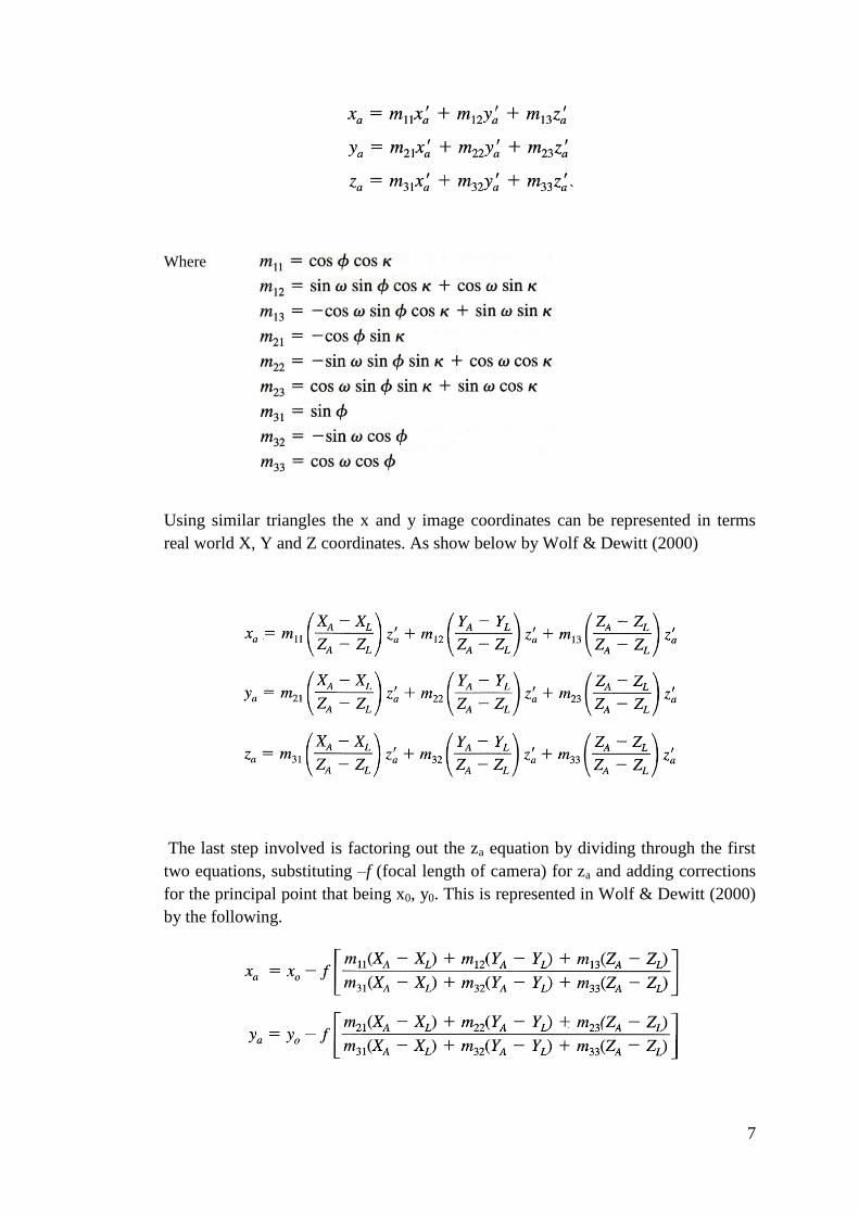
Wolf & Dewitt (2000) present the following rotation equations.
7
`
Where
Using similar triangles the x and y image coordinates can be represented in terms
real world X, Y and Z coordinates. As show below by Wolf & Dewitt (2000)
The last step involved is factoring out the za equation by dividing through the first
two equations, substituting –f (focal length of camera) for za and adding corrections
for the principal point that being x0, y0. This is represented in Wolf & Dewitt (2000)
by the following.

8
This equation can be used to transform real world coordinates onto the photo image
coordinates if the following six variables (described by Wolf & Dewitt (2000) as ‘the
six elements of exterior Orientation’) and two constants are known. The first three
variables are the coordinates of the exposure station (where the photo is taken),
represented by XL, YL & ZL; the next three variables are the omega, phi and kappa
rotations, represented by the m coefficients; the constant focal length of the camera
which is available in the camera specifications. Lastly the principle point of the
photo which can be worked out as it is the exact middle of the photo coordinates.
TWolf & Dewitt (2000) detail a way to solve those six variables, or as Wolf &
Dewitt (2000) call ‘six elements of exterior orientation’, of a photograph which is
named ‘space resection by collinearity’.
2.4 Methods for Solving the Six Elements of Exterior Orientation
There are different ways to ascertain some approximate solutions which can be
worked out rigorously to provide better solutions. Grussenmeyer & Khalil (2002)
document five different ways to gain an approximate solution, each has their own
requirements and are discussed in the following.
Firstly is the Direct Linear Transformation (DLT) which can be solved without
initial approximations. The equations require 11 unknown parameters to be solved
which can be solved iteratively if six points are coordinated provided that they aren’t
on the same plane.
Second is the Church Method which is an application of the coangularity condition,
requires at least three control points and can derive the solution from a single photo.
This method requires initial approximations and can account for image distortion if
four or more control points are available so the least squares method can be applied.
The third and fourth methods are to be applied to models rather than an image and
are not applicable to this project. The final method is under the title, approximate
solution for spatial transformation. It requires four points to be known in both the
image and real world coordinate system.
Wolf & Dewitt (2000) present anther idea which is called space resection by
collinearity which is the method adopted for this project. For this space resection
method to work a minimum of three control points must be visible on the photograph.
These control points must be fixed onto a real world coordinate system. From this,
the unknown variables can be solved using the collinearity equations. A key
consideration when using this method is the fact that initial approximations are
required for the six element of exterior orientation. This is because the collinearity
condition equations are non-linear and to make this method work Wolf & Dewitt
(2000) have adopted Taylor’s theorem to lineraise them and produced the equations
below.

9
2.5 Space Resection by Collinearity
The calculations involved in the space resection method are prohibitive time-
consuming to do by hand. So it is a prime candidate for computer programming as it
a method with multiple iterations, as a correction is applied to the current value each
loop of calculations. That being said the first thing needed before starting this
method is the focal length of the camera and initial approximations for the six
exterior orientations.
2.5.1 Focal Length
The focal length is a very important value in this method and can change results
dramatically if incorrect. The focal length of a camera is not standard across all
cameras so to ascertain the correct value the cameras specifications should be
researched. On top of that the focal length needs to be related correctly to the
coordinate system adopted for the photograph.
The focal length stated in the specifications does not reflect the focal length required
in this method, but is used to calculate the required value. The value in this method
also requires the knowledge of the image sensor type, and with this information the
image sensor size can be ascertained. These names and dimensions of the image
sensors were first used to standardise TV camera tubes and has carried over to now
(Bockaert, 2003).
The sensor are named after a fraction of an inch (e.g. 1/2.7”), or a dimension in
millimetres (e.g. 35mm) and sometime followed by CCD (Charge-coupled) device or
CMOS (Complementary metal–oxide–semiconductor). This length has no
mathematical relationship to the actual image sensor size it is just the diameter of the
circle around the sensor as seen in the figure 2.3 below. So to find the corresponding
image sensor sizes research is required into the standardised measurements. Below in
Table 2.1 is a list of some commonly used cameras.
Figure 2.3 Image Sensor Types (Bockaert, 2003)

10
Table 2.1 Common Image Sensor Sizes (Bockaert, 2003)
The percentage difference between the coordinate system extents of the photo and
the sensor size need to be applied to the focal length stated in the specifiactions.
2.5.2 Initial Approximations
Wolf & Dewitt (2000) use equations derived from Pythagoras Theorem and a two
dimensional conformal coordinate transformation to approximate the exposure
stations real world coordinates. These methods have not been used in this project and
the reason is explained in Chapter 3. Wolf & Dewitt (2000) do ‘compute two
dimensional conformal coordinate transformation parameters by a least squares
solution’ to solve for the omega, phi and kappa rotations. These equations are shown
in matrix form below, as if it was only using three points to solve. The values a and b
in Matrix X can be used to calculate the initial approximations of the rotations.
Where

11
2.5.3 Solving the Six Exterior Orientation Parameters
The process in which this method comes to the correct answer is by apply
corrections to the initial approximations and repeat with the new approximations
until the corrections become insignificant. The next step is to use the linearised
equations shown in section 2.4 and represent them in matrix form as show below.
The normal equation of this is
Where

12
The equations for the m’s are is Section 2.3. After these calculations are completed
the results are in a matrix and it provides the omega, phi, kappa, XL, YL and ZL
corrections. As noted before this step is repeated until the corrections are
insignificant, and with a computer program it only takes a few seconds to run
through this one hundred times which is more than enough.
2.6 Augmented Reality Control Methods
The control used in this project is a detrimental factor in the success of this project.
Haller, Billinghurst & Thomas (2007) argue that computer vision methods of control
are the only ones that have ‘the potential to yield non-invasive, accurate, and low-
cost solutions’. Predefined marker methods and the use of natural features as
markers are the best suited methods for this project.
Haller, Billinghurst & Thomas (2007) introduces two predefined marker methods,
one using point-like markers and one using extended markers. The point-like marker
method proposes that circular markers are the best, because they are easily
identifiable, the least affected by perspective distortion and provide a stable 2D
position. There are many different approaches to the make-up of the circular marker,
but mainly they consist of 3 or 4 concentric circles with contrasting colours, such as
black and white. A number of these markers would be placed around the scene and

13
there real world position worked out. Then the centre point of each marker would be
used to retrieve the camera pose.
Extended markers come in all shapes and sizes but generally consist of a black
square with some detail in the middle, such as white text or white and black shapes.
See figure 3.3 for an example of a basic marker.
Figure 2.4 Basic AR Marker
This marker has enough detail to estimate the pose, as the corners of the squares and
rectangle as well as the centre of the circle is used for the control. The use of these
markers are becoming more popular with the public and even with advertisers as it
produces good results and software is freely available enabling anyone to create their
own AR experience.
Haller, Billinghurst & Thomas (2007) also introduces two approaches to using
natural features as markers (markerless AR), the edge based method and the texture
base method. An edge based will basically recognise strong edges, such as edges on
a building, and compare the computer estimated edges with the 3D model to work
out the camera pose. This method has its drawbacks especially with lighting, because
shadows cast can create strong enough line to confuse the system. The texture
method relies on being able to match interest points in the scene to the 3D model.
All these control methods only use points and/or lines in the cameras view to
calculate the camera pose. So if the position of the camera, when the photograph is
taken, is knows in relation to the 3D model coordinate system this would cut down
on amount of control needed and also improve on results. The positions could easily
be measured off the structures and/or boundaries close by to achieve a good position
fix.

14
2.7 Augmented Reality Authoring Tools
An AR authoring tool is a tool designed to enable people with specific skills to be
able to create their own AR experience. Seichter, Looser & Billinghurst (2008)
presents the idea that there are three levels of AR authoring tools. The lowest level
include tools like software libraries the prime example of this is ARToolkit, which is
the most well-known and used. In order to develop from these lower level tools
expert programming skills are required as well as a link to be developed between the
library and the virtual data. MATLAB even though it is not dedicated to AR
technology would also fall into this category as it has the capacity to build an AR
system and requires extensive programming to develop it.
The next level AR authoring tool doesn’t involve as much programming as the
lowest level but it still requires a proficient programmer to develop the AR system to
completion. Examples of these next level tools are libraries such as OSGAR and
Studierstube.
The final level includes GUI-based (graphical user interface) tools, which are tools
for developers with no programming skills. The tools that are existing in this
category can have different approaches, some are created as an add on to existing 3D
modelling programs, like google sketch up. While other tools use an environment
where programming can be done visually and modified it to support AR input.
Seichter, Looser & Billinghurst (2008) proposes an authoring tool that ‘supports
both scripting and a drag and drop interface, real time interpreted input, and allows
users to add functionality depending on their needs’.
2.8 Augmented Reality Projects
This project is unique due to the fact it aims at producing a product that deals only
with photos and uses human input to identify markers. It is a simpler version of some
existing AR projects, but still will produce something that will be beneficial to
certain people/business involved in construction. Assuming that the computer design
data is provided by the engineer or architect that is designing the building or
extensions.
Project that are similar to this one include, Georgel, P et al. (2009) which is a paper
that presents a photo-based augmented reality system designed for industrial
application. The paper details their methods of automatically estimating the pose
which can be used for direct augmentation. This work could be built upon and or
used as a guide to achieving the project aim.
Also another similar project is, Woodward et al. (2010) who present their project
AR4BC (Augmented Reality for Building and Construction) which is a detailed

15
description of their mobile AR software system. The project displays 3D modelling
data onto a live video feed which is done by placing the virtual data correctly onto
the video feed using markers and then locking it into position. So as you move the
virtual data is locked into position and essentially stays in position in the real world
as the camera is moved around. The paper has some excellent ideas and approaches
that could applied for this project.
2.9 Conclusion
This research has led to identifying the best procedures, systems and programs to
utilise when carrying out the aims of this project. All the procedures, systems and
programs have been put to the test in different conditions and have provided good
results. Now these selected components will be used in a different way and test out
whether or not they will produce an acceptable solution.
Although there is big business involved in augmented reality for construction this
project will provide a different way to produce AR and also testing how accurate it
can be. This will therefore lead to conclusion on what other applications AR could
be used for.

16
CHAPTER 3
METHOD
3.1 Introduction
This chapter states the research objectives and sets out the methods and procedures
that were followed to enable the development of an AR program that is capable
plotting design data onto a digital photo. It will also document the field testing
undertaken and discuss the methods and procedures used to obtain the field data.
The testing involved must be thorough and where possible follow commonly used
and well tested techniques to ensure the quality of the results is satisfactory and to
ensure the validity of it use for future users.
3.2 Research Objectives
These research objectives listed below are the guide to what needs to be
accomplished in order for the project aims to be met.
The objectives that need to be meet are:
Gain an understanding of MATLAB to the point where a basic AR program
can be written.
Research the photogrammetry principles that will form the algorithm in the
program.
Develop the program part by part i.e. user input, algorithm and output.
Choose appropriate test sites that test different scenarios that could arise in
the construction industry.
Develop a sound testing technique that is thorough and has inbuilt checks.
Analyse the test results accounting for the variables and errors that could
arise.
Compare results across the different sites used.

17
3.3 MATLAB Basics
The software that has been used for the project is MATLAB student version, version
7.12.0.635.
Figure 3.1 General MATLAB Information
Figure 3.2 Typical MATLAB Layout

18
Mathworks states that ‘MATLAB is a high level technical computing language and
interactive environment that enables you to perform computationally intensive tasks
faster than with traditional programming languages such as C, C++, and Fortran’.
MATLAB can be used for many applications from solving any mathematical
problems to processing images. The basic layout as seen above consists of four
windows. First the command window in the centre is where instructions are entered.
Next is the bottom right window and is where you can see all the previously entered
commands. To the left is the Current Folder Window where all the scripts and other
files used, like a photo, is going to be accessed from. Finally in the top right is the
workspace window and contains all the MATLAB data that has been created during
the current session. MATLAB will open a new window to allow the programming
script to be written.
3.4 Programming the Algorithm
Firstly the program need to be able to facilitate data for the focal length, the real
world coordinates for the control points and the design data. This is just a matter of
assigning these to their own matrix so it can be called upon later. Below is an
example of what is required. The columns are represented by X value, Y value and Z
value respectively.
data = [2499.461 5020.228 100.496
2502.653 5019.768 100.613
2505.971 5019.210 100.726
2505.152 5012.928 100.728 ]
When developing a program the variable input needs to be considered. In this
instance the variable input will be the different amount of control points that will be
used from picture to picture. Some photos will only have 3 points while other could
have 10. The more control point used, the more equations will need to be formed. To
compensate for this, the algorithm developed for this project has built in loops that
will generate the correct amount of equations based on the control points.
L81 = [];
for counter4 = 1:NumOfCtrlPts (1,2)
L81temp = [ CtrlCoord(counter4,3)
CtrlCoord(counter4,4)];
L81 = [L81;L81temp];
end

19
As you can see in the code extracted from the project algorithm I first create a
variable outside the loop which has nothing in the matrix. Then the program enters
the loop and will go through the loop the number associated with ‘NumOfCtrlPts’
which is the number of control point used. Inside the loop it creates a matrix
‘L81temp’ which is a temporary matrix that gets overridden each loop. This matrix is
used to build ‘L81’ with all the values of each loop stacked into one matrix.
Next issue to consider is having the ability to only need the input in the one place.
This is done by creating all the matrices at the start and throughout the script a single
value in a certain matrix can be called on to be used. In the example above you can
see that in the first line of ‘L81temp’ it calls on the matrix ‘CtrlCoord’, and reference
after is the row and column of the matrix. In this instance the row is equal to what
number the loop is up to and it will call the third column each loop. As the algorithm
develops further the values needed to be used will come from newly created data,
which can be called on the same way. This is apparent in the example just before, as
the matrix ‘CtrlCoord’ has been formed from the original input data and now is
being used for the ‘L81temp’ matrix.
The rest is fairly straight forward as MATLAB handle mathematical equations very
well. It understands all the trigonometric functions like sine cosine and tangent. It
handles all sort of matrix mathematics like multiplication, transposing, inversing etc.
For example here are the mathematical equations represented in the projects code.
triangle = (B' * B)^-1 * (B' * epsilon);
m11 = cos(phi)*cos(kappa);
m12 = sin(omega)*sin(phi)*cos(kappa )+ cos(omega)*sin(kappa);
m13 = - cos(omega)*sin(phi)*cos(kappa)+ sin(omega)*sin(kappa);
m21 = -cos(phi)*sin(kappa);
m22 =– sin(omega)*sin(phi)*sin(kappa)+ cos(omega)*cos(kappa);
m23 = cos(omega)*sin(phi)*sin(kappa) + sin(omega)*cos(kappa);
m31 = sin(phi);
m32 = -sin(omega)*cos(phi);
m33 = cos(omega)*cos(phi);
20
Lastly of note in the coding of the algorithm, to help with analysis a loop was built in
to create all the calculated values using all the different combination of control
marks. For example one site has nine control marks, the program can test all the
different combinations using only four of the nine. The program compiles all the
results together which is ideal for the analysis as it compares control that is used in
different areas.
The space resection by collinearity requires initial approximations and as stated in
Chapter 2 the equations to gain an initial coordinate approximation are not used in
this program. The reason for this is that because the application of this program is
mostly suited to construction jobs the photos will not be taken very far away from
the control points. Therefore it would be accurate enough to measure with a tape or
even pace out to the exposure station as this would be accurate enough for the
program. Also with the height generally the photo would be taken around the same
height of the control marks so adopting the average height of the control marks
would be satisfactory. If for some reason the heights are significantly different a
good guess would also be satisfactory as the iterative process will still achieve the
correct answer. As long as the values of all initial approximations or within a certain
range the program can solve it. Once outside the range the program will not solve
and in fact the more iterations that take place the further away from the correct
answer it will be. These ranges will be discussed in chapter 5.
3.5 Programming to Accept User Input
One of the main aims of this project is to automate the process from start to finish.
The only manual part is the loading in of the control points and the design data. The
process in which the photo coordinates are derived is by clicking the corresponding
control points in the correct order on the actual photo. The program recognises where
the mouse is when the button is clicked and stores that information in the correct
spot for calculations. The other feature that is programmed is the plotting of the point
that was just clicked, this is to show exactly where the mouse clicked and also to
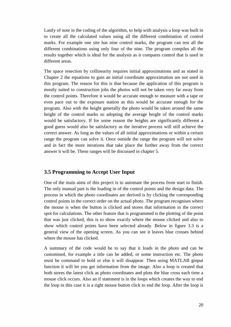
show which control points have been selected already. Below in figure 3.3 is a
general view of the opening screen. As you can see it leaves blue crosses behind
where the mouse has clicked.
A summary of the code would be to say that it loads in the photo and can be
customised, for example a title can be added, or some instruction etc. The photo
must be command to hold or else it will disappear. Then using MATLAB ginput
function it will let you get information from the image. Also a loop is created that
both stores the latest click as photo coordinates and plots the blue cross each time a
mouse click occurs. Also an if statement is in the loops which creates the way to end
the loop in this case it is a right mouse button click to end the loop. After the loop is

21
ended the photo is closed down and then the algorithm runs through with this input
and plots out the design data onto the same photo.
As with most programs this is still a work in progress and also could be made more
efficient by using different function calls and other approaches. The main issue with
the first step in the program is when you are required to click the control points the
ability to zoom into the photo isn’t there. Sometimes the control points are small and
to be able to zoom would be a good feature. The needs further research and the
projects timeframe didn’t enable this to happen.
Figure 3.3 Initial View

22
3.6 Programming to Plot Lines onto the Photo
To be able to plot design data onto the photo the user must provide a list of real
world coordinates and also the start and end points of the lines. Using the start and
end points the program can plot the lines from one coordinate to the other. Below is
an extract of code of what is to be provided. First column is the X value, next
column is the Y value and the last column is the Z value
RWC = [ 2500.884 5009.932 102.5
2504.659 5013.294 102.5
2498.537 5012.568 102.5
2502.398 5011.28 100
2502.398 5011.28 102 ]
Below is an example of the data needed for the lines. The first column is the start
point and the second is the end point.
linestojoin = [ 8 9
8 20
5 4
5 6
19 9 ]
Once all the required data is plugged in the output is plotted onto the original photo.
A typical example is shown below.
Figure 3.4 Typical Output

23
3.7 Field Testing
The field testing that was undertaken for this project involved access to the following
materials. A digital camera to obviously take the photos but the focal length needed
to be accessible. The camera used in this project was Fujifilm FinePix S5500. Below
is a picture of the camera itself and the specifications table in the owners’ manual.
Figure 3.5 Project Camera
Table 3.1 Project Camera Specifications
The next item required are the targets that must, stand out from the background,
easily recognisable in the photo, be easily placed onto the site be a solid mark for
multiple measurement to be taken to them. On one site dumpy pegs and stakes were
used as control marks and on the other two site a paper target was used as depicted in
Figure 3.6.
Figure 3.6 Target for control points

24
To obtain the real world coordinates a Topcon 9000 total station was used. This was
used in conjunction with a controller and a prism.
The procedures followed in the field are as follows. To gain enough redundant
checks on the data it was decided that 40 marks would be placed, some for the
control marks and the rest as redundant shots. They were spread over the whole site
and not in a uniform manner to create some randomness to it. First step was to place
the targets in the appropriate places, trying to get to the full extents of the photo.
Next step was to take photos of the site with as many if not all the target in site.
Photos were taken from multiple points around each site and different angles were
utilised. Finally the total station would be set up and radiated to all the points. All
radiations used both faces. The total station would then be set on another station and
radiate all the points again so there would be redundant check shots.
3.8 Sites Chosen
The testing was done on three different sites each with their own unique features, so as to
test different scenarios and factors that could affect the quality of the output. One site was
indoors, another site was outdoors with a building on it and the last was vacant outdoor site.
Below are picture of each site.
Figure 3.7 Indoor Site (Site 1)

25
Figure 3.8 Outdoor Building Site (Site 2)
Figure 3.9 Outdoor Vacant Site (Site 3)
3.9 Testing the program
As with most programming there will be glitches that need ironing out, especially if
the programmer is inexperienced. A good start to testing the program is using these
different field scenarios as different inputs and parameters will be needed on each
site and with each view.
To test for the accuracy of the data output the field data will be put through the
program and a statistical analysis will be carried out. This will include comparing the
differences of the calculated photo points and the actual photo points. Other

26
calculations will be carried out such as the standard deviation of the residual
differenced and calculate the 95% confidence interval of the error differences. This
will be a good indicator on how accurate the system is and under what conditions it
struggles.
3.9 Conclusion
In order to effectively test and analyse the projects program these three different site
have been chosen and each with a good amount of redundant check shots.

27
CHAPTER 4
DATA ANALYSIS
4.1 Introduction
This chapter will discussed the results of the field work reduction and display all the
findings that were gathered from the tests that were discussed in chapter 3. This
information provided in this chapter will be the values of interest, as there was a lot
of analysis completed but is not necessary for the report as for example some of the
tests didn’t achieve any results as it was beyond the limitations of the system, this
will however discussed in chapter 5.
This chapter will go through the sites in order discussing each view one at a time and
pointing out the problems occurred along the way. Most views have multiple results
as two different amounts of targets were used to ascertain the results. Under each
view and amount of control the following will be presented. The data will be
represented by the difference in the x photo coordinate and the y photo coordinate. A
note to keep in mind is that the photos taken are on a coordinate system that is 2272
pixels along the x axis and 1704 pixels along the y axis. Each site will show results
of minimums and maximums coordinate difference. The mean and standard
deviation will be obtained in order for the 95% confidence interval to be calculated.
A note to remember the 95% confidence interval is plus or minus from the
population mean.
4.2 Field Work Reduction
As discussed in the previous chapter the targets were radiated by a theodolite, from
two different station and using both the left and right face. The results of the field
work were more than satisfactory as all the checks came within millimetres. During
the reduction process an error in the prism heights were found on a few targets. The
correct height was adopted and the heights were adjusted correctly. The coordinates
of all the targets can be found in the Appendix.
4.3 Test Site 1 – Indoor site
In this section the results of three different views will be discussed. The first view
was straight on and can be seen above in figure 3.7. The other two were from the

28
sides and due to the angle some target cannot be seen. These can be view in the
appendix.
4.3.1 Test Site 1 – View 1
This straight on view had a good view of all targets except one as it was hard to
pinpoint as the glare of the sun masked it. Firstly the results from using eight targets
as control points are as follows.
Mean -0.58015
Mean -1.06222
Standard deviation 8.541948
Standard deviation 4.893036
95% Confidence Interval 3.029
95% Confidence Interval 1.735
Minimum -18.5293
Minimum -19.0413
Maximum 14.43207
Maximum 8.970447
Number of Residual Targets 32
Number of Residual Targets 32
X values Y values
Now the results from using five control points
Mean -6.09207
Mean -5.50369
Standard deviation 9.264519
Standard deviation 5.788793
95% Confidence Interval 3.285
95% Confidence Interval 2.053
Minimum -19.7029
Minimum -22.5612
Maximum 8.332693
Maximum 8.928934
Number of Residual Targets 32
Number of Residual Targets 32
X values Y values
4.3.2 Test Site 1 – View 2
This view was side on and because of the angle some targets were obstructed.
Results were only obtained using six targets.
Mean -1.29026
Mean -1.28805
Standard deviation 6.782353
Standard deviation 5.667839
95% Confidence Interval 2.405
95% Confidence Interval 2.010
Minimum -10.7178
Minimum -19.4049
Maximum 7.638602
Maximum 6.0905
Number of Residual Targets 20
Number of Residual Targets 20
X values Y values

29
4.3.3 Test Site 1 – View 3
This view was again side on and because of the angle some targets were obstructed.
Results were only obtained using six targets.
Mean -1.53376
Mean -0.55319
Standard deviation 7.882727
Standard deviation 7.034946
95% Confidence Interval 2.795
95% Confidence Interval 2.494
Minimum -14.6039
Minimum -22.7173
Maximum 12.78307
Maximum 8.740348
Number of Residual Targets 17
Number of Residual Targets 17
X values Y values
4.4 Test Site 2 – Outdoors with building
This site was outside and targets were placed on to the side of a building and the
results of the three views will be presented below.
4.4.1 Test Site 2 – View 1
This view could see all targets with a few hard to pinpoint because of the angle and
also being careful not to use the reflection of a target in the window. First results are
from using eight control points.
Mean -0.40145
Mean -1.32373
Standard deviation 3.949598
Standard deviation 2.377611
95% Confidence Interval 1.400
95% Confidence Interval 0.843
Minimum -6.20277
Minimum -6.61567
Maximum 8.58069
Maximum 4.78585
Number of Residual Targets 32
Number of Residual Targets 32
X values Y values
Now the results from using five control points
Mean 3.453268
Mean 4.048562
Standard deviation 2.713303
Standard deviation 8.393211
95% Confidence Interval 0.962
95% Confidence Interval 2.976
Minimum -1.40477
Minimum -8.95371
Maximum 10.77053
Maximum 18.35445
Number of Residual Targets 32
Number of Residual Targets 32
X values Y values
30
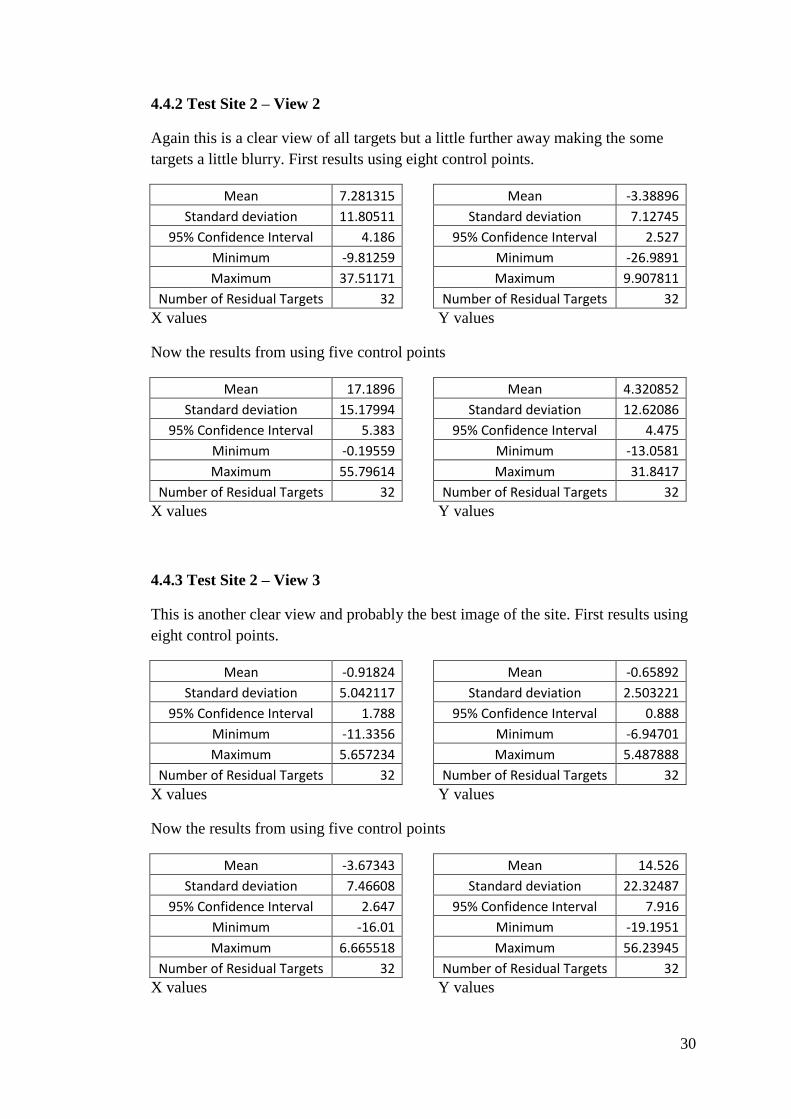
4.4.2 Test Site 2 – View 2
Again this is a clear view of all targets but a little further away making the some
targets a little blurry. First results using eight control points.
Mean 7.281315
Mean -3.38896
Standard deviation 11.80511
Standard deviation 7.12745
95% Confidence Interval 4.186
95% Confidence Interval 2.527
Minimum -9.81259
Minimum -26.9891
Maximum 37.51171
Maximum 9.907811
Number of Residual Targets 32
Number of Residual Targets 32
X values Y values
Now the results from using five control points
Mean 17.1896
Mean 4.320852
Standard deviation 15.17994
Standard deviation 12.62086
95% Confidence Interval 5.383
95% Confidence Interval 4.475
Minimum -0.19559
Minimum -13.0581
Maximum 55.79614
Maximum 31.8417
Number of Residual Targets 32
Number of Residual Targets 32
X values Y values
4.4.3 Test Site 2 – View 3
This is another clear view and probably the best image of the site. First results using
eight control points.
Mean -0.91824
Mean -0.65892
Standard deviation 5.042117
Standard deviation 2.503221
95% Confidence Interval 1.788
95% Confidence Interval 0.888
Minimum -11.3356
Minimum -6.94701
Maximum 5.657234
Maximum 5.487888
Number of Residual Targets 32
Number of Residual Targets 32
X values Y values
Now the results from using five control points
Mean -3.67343
Mean 14.526
Standard deviation 7.46608
Standard deviation 22.32487
95% Confidence Interval 2.647
95% Confidence Interval 7.916
Minimum -16.01
Minimum -19.1951
Maximum 6.665518
Maximum 56.23945
Number of Residual Targets 32
Number of Residual Targets 32
X values Y values
31
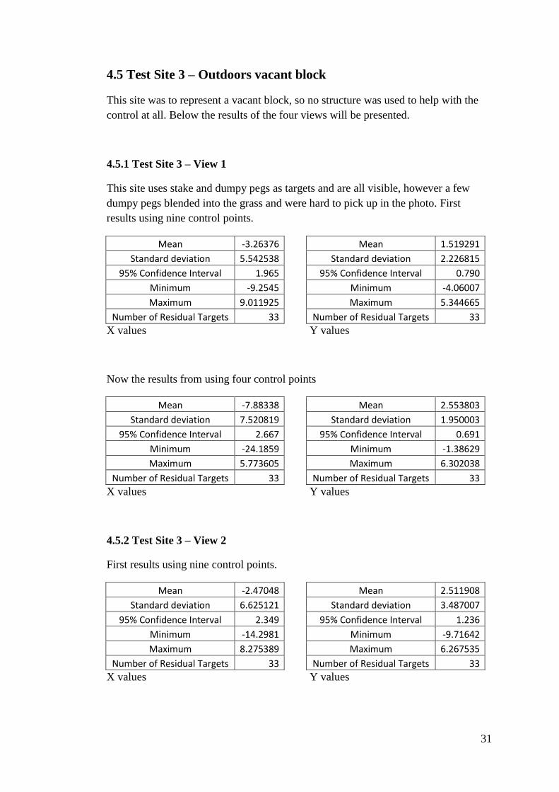
4.5 Test Site 3 – Outdoors vacant block
This site was to represent a vacant block, so no structure was used to help with the
control at all. Below the results of the four views will be presented.
4.5.1 Test Site 3 – View 1
This site uses stake and dumpy pegs as targets and are all visible, however a few
dumpy pegs blended into the grass and were hard to pick up in the photo. First
results using nine control points.
Mean -3.26376
Mean 1.519291
Standard deviation 5.542538
Standard deviation 2.226815
95% Confidence Interval 1.965
95% Confidence Interval 0.790
Minimum -9.2545
Minimum -4.06007
Maximum 9.011925
Maximum 5.344665
Number of Residual Targets 33
Number of Residual Targets 33
X values Y values
Now the results from using four control points
Mean -7.88338
Mean 2.553803
Standard deviation 7.520819
Standard deviation 1.950003
95% Confidence Interval 2.667
95% Confidence Interval 0.691
Minimum -24.1859
Minimum -1.38629
Maximum 5.773605
Maximum 6.302038
Number of Residual Targets 33
Number of Residual Targets 33
X values Y values
4.5.2 Test Site 3 – View 2
First results using nine control points.
Mean -2.47048
Mean 2.511908
Standard deviation 6.625121
Standard deviation 3.487007
95% Confidence Interval 2.349
95% Confidence Interval 1.236
Minimum -14.2981
Minimum -9.71642
Maximum 8.275389
Maximum 6.267535
Number of Residual Targets 33
Number of Residual Targets 33
X values Y values
32
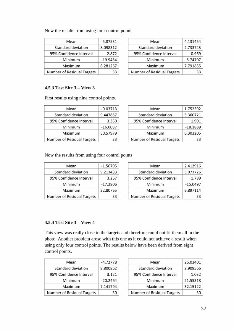
Now the results from using four control points
Mean -5.87531
Mean 4.131454
Standard deviation 8.098312
Standard deviation 2.733745
95% Confidence Interval 2.872
95% Confidence Interval 0.969
Minimum -19.9434
Minimum -5.74707
Maximum 8.281267
Maximum 7.791855
Number of Residual Targets 33
Number of Residual Targets 33
4.5.3 Test Site 3 – View 3
First results using nine control points.
Mean -0.03713
Mean 1.752592
Standard deviation 9.447857
Standard deviation 5.360721
95% Confidence Interval 3.350
95% Confidence Interval 1.901
Minimum -16.0037
Minimum -18.1889
Maximum 30.57979
Maximum 6.303205
Number of Residual Targets 33
Number of Residual Targets 33
Now the results from using four control points
Mean -1.56795
Mean 2.412916
Standard deviation 9.213433
Standard deviation 5.073726
95% Confidence Interval 3.267
95% Confidence Interval 1.799
Minimum -17.2806
Minimum -15.0497
Maximum 22.80765
Maximum 6.897114
Number of Residual Targets 33
Number of Residual Targets 33
4.5.4 Test Site 3 – View 4
This view was really close to the targets and therefore could not fit them all in the
photo. Another problem arose with this one as it could not achieve a result when
using only four control points. The results below have been derived from eight
control points.
Mean -4.72778
Mean 26.03401
Standard deviation 8.800862
Standard deviation 2.909566
95% Confidence Interval 3.121
95% Confidence Interval 1.032
Minimum -20.2464
Minimum 21.55318
Maximum 7.141794
Maximum 32.15122
Number of Residual Targets 30
Number of Residual Targets 30

33
4.6 Testing the Limitations of the Program
In order to test the limitation of the program the critical parameters that could make
the program not return a value must be known. The critical parameters are the initial
approximations of omega, phi, kappa, XL, YL and ZL. Another critical parameter is
the focal length as it is many of the equations throughout the method it can send it
past being able to achieve a result. The other factors that play a critical role are the
input parameters. These include the real world coordinates of the control points and
their corresponding photo coordinates.
To test these parameters it was setup with known answers and then to see the effect
of a single parameter it would be change slightly to see how the program reacts. The
space resection can deal with wrong approximations to a point but when it reaches its
range the iteration make the solutions worse each loop. For these test done for the
project it has been found that with as error of about +/- 5m for the initial
approximation the program could handle that is if the rotation is correct. In the case
of rotation a single parameter can be out about 30-40 degrees before issues start to
aries.
4.7 Conclusion
The results achieved here in this testing have been gathered across different sites and
using different types of control and different amounts and provide a good insight into
what the application could be used for and how best to use it.

34
CHAPTER 5
DISCUSSION AND CONCLUSIONS
5.1 Introduction
The results shown in chapter four have provided the first look into how accurate this
system can be. This chapter will further analyse and discuss the implication of the
results. The tests performed are by no mean a complete test on the accuracy but it
has provided a good basis to begin with.
This chapter will delve into how the program performed, identify any glitches that
will need further work, and provide insight into the reasons of some of the less
accurate results.
5.2 Results Discussion
The purpose of this AR application is to provide a good visualisation tool to
people/business involved with the construction industry. That being said the results
should be discussed in relation to the application it will be used for and there is no
real high accuracy needed. So generally for the purpose it would serve the accuracy
would be adequate. This section will discuss each site in further detail.
5.2.1 Site 1 results discussion
Site produced some very good results here mainly because the site was smaller and
the photos could be taken at a closer distance making the targets clearer. The highest
differential population mean was -6 with a 95% CI of +/- 3.285. To put this into
perspective the units that are being dealt with are pixels. With these image being
2272 x 1704 image size a mean of -6 and +/- 3.285 is very good for a visualisation
tool. To relate it back to mm it is approximately 10 pixels cover about 50mm at a
when if the object is about 15m away.
One thing for discussion is the outliers in some of those minimums and maximums.
Two things could be happening here. One the target in question with the larger
discrepancy could be closer to the camera and resulting in a smaller real world
distance. The other issue encountered is when the targets are 2D objects and the
camera is moved to an awkward angle and it makes it hard to identify and accurately
obtain the photo coordinate.
The other interesting point that comes out of site one is the comparison using eight
control marks, six control marks or five control marks. At this site it clearly gets
better with more control marks. But that it not to say the more the better, as they

35
must be positioned appropriately or else it will defeat the purpose of have extra
control.
5.2.2 Site 2 Results Discussion
The thing that first jump out of the results are the comparisons between the 3 views
using only 5 control marks. This really back up that position of the targets is key
rather that quantity. As you can see in view 1 the five control marks performed
reasonably well but in view 2 and 3 the accuracy drops off significantly. The same
five control point were used for each view so it suggests that a better positioned
target in the other two view would have done the results a great deal of good.
Here again the eight control mark outperformed the five, this is probably more
prevalent on this site because of the different faces of the building the image covered.
5.2.3 Site 2 Results Discussion
Again the test with more control marks came up with better results. The issue for
discussion that came out of site three is that the code didn’t handle view four very
well. That is the initial approximation for the rotations angles so they were put is
manually. This could have arisen from some bad data being plugged in or a matter of
a coding issue.
5.3 Future Work
There is plenty of future work that could be done but would require some good
programming skills. The idea to take this further and using this as a base to create a
live video feed augmented reality system. The extent of the programming only
enables to plot a wireframe of a building over the picture. Investigation into what is
involved is rendering the picture could be a good place to head. Further automate the
system and allow for more user friendly input.
5.4 Conclusion
This project has developed an AR system with MATLB and has tested the accuracy
of the outputs. This can hopefully lead to some AR technologies ending up in the
survey industry.

36
LIST OF REFERENCES
Abi research, 2011, Augmented Reality-Enabled Mobile Apps Are Key to AR Growth,
Abi research, Oyster Bay, USA, viewed 19 May 2011,
<http://www.abiresearch.com/press/3614-Augmented+Reality-
Enabled+Mobile+Apps+Are+Key+to+AR+Growth>
ARToolworks, 2007, ARToolworks Inc, Seattle, USA, viewed 20 May 2011,
<http://www.hitl.washington.edu/artoolkit/>
Behringer, R, Klinker, G & Mizell DW 1999, Augmented Reality—Placing Artificial
Objects in Real Scenes, Proceedings of IWAR '98, A K Peters, Natick,
Massachusetts, USA.
Bimber, O & Raskar, R 2005, Spatial Augmented Reality : Merging Real & Virtual
Worlds, A K Peters, Natick, Massachusetts, USA.
Bockaert, V 2003, Sensor Sizes, Digital Photography Review, UK Viewed 20
October 2011, <http://www.dpreview.com/learn/?/key=sensor+sizes>
Cassella, D 2009, What is Augmented Reality (AR): Augmented Reality Defined,
iPhone Augmented Reality Apps and Games and More, Digital Trends, Portland,
viewed 20 May 2011, <http://www.digitaltrends.com/mobile/what-is-augmented-
reality-iphone-apps-games-flash-yelp-android-ar-software-and-more>
Georgel, P, Benhimane, S, Sotke, J & Navab, N 2009, Photo-based Industrial
Augmented Reality Application Using a Single Keyframe Registration Procedure,
IEEE International Symposium on Mixed and Augmented Reality 2009 Science and
Technology Proceedings, 978-1-4244-5419-8/09, p. 187 & 188.
Haller, M, Billinghurst, M & Thomas, B 2007, Emerging Technologies of
Augmented Reality: Interfaces and Design, Idea Group, Hershey, USA.
Lonescu, H 2010, 6DOF, Wikipedia, Viewed 20 October 2011,
<http://en.wikipedia.org/wiki/File:6DOF_en.jpg>
Roberts, D 2011, Making things move, McGraw-Hill, New York.
Seichter, H, Looser, J & Billinghurst, M 2008, ComposAR: An Intuitive Tool for
Authoring AR Applications, IEEE International Symposium on Mixed and
Augmented Reality 2008 Science and Technology Proceedings, 978-1-4244-2859-
5/08, p. 177 & 178.
Sung, D 2011, The history of augmented reality, Pocket-lint, Ascot, viewed 20 May
2011, <http://www.pocket-lint.com/news/38803/the-history-of-augmented-reality>

37
Wolf, PR & Dewitt, BA 2000, Elements of Photogrammetry: with Applications in
GIS, 3rd
edn, McGraw-Hill, USA.
Woodward, C, Hakkarainen, M, Korkalo, O, Kantonen, T, Aittala, M, Rainio, K &
Kähkönen, K 2010, Mixed Reality for Mobile Construction Site Visualization and
Communication, 10th International Conference on Construction Applications of
Virtual Reality, VTT Technical Research Centre of Finland.

38
APPENDICES
.

39
APPENDIX A
University of Southern Queensland
FACULTY OF ENGINEERING AND SURVEYING
ENG 4111/2 Research Project PROJECT SPECIFICATION
FOR: DANIEL KENNETH MAHER
TOPIC: PROJECTION OF COMPUTER DESIGN DATA ONTO
DIGITAL PHOTOGRAPHS
SUPERVISOR: Glenn Campbell (USQ Supervisor)
PROJECT AIM: This project aims to develop a program that will automate the
superimposing of computer design data over photos and testing field
data to acquire an accuracy range..
SPONSORSHIP: None
PROGRAMME: Issue A. March 2011
1. Research literature relating to augmented reality devices and investigate how they
work and what hardware is used.
2. Develop and implement an algorithm to project 3D model onto a 2D digital
photograph.
3. Use simulations to investigate the effect of control on the model projection.
4. Apply the algorithm to three study sites.
5. Investigate what hardware and software would be necessary to implement this in a
consumer device.
6. Prepare and submit the final dissertation.
As time permits:
7. Investigate the possibility of developing a real time system.
AGREED:
(Student) (Supervisor)
Dated: __ / __ / __ __ / __ /__

40
APPENDIX B

41
APPENDIX C
%input stuff f = 2408.9596;
%control points data = [2499.461 5020.228 100.496 2502.653 5019.768 100.613 2505.971 5019.210 100.726 2505.152 5012.928 100.728 2502.173 5013.051 100.598 2498.981 5014.270 100.537 2497.887 5009.227 100.572 2502.218 5007.688 100.687 2505.090 5008.746 100.805];
datasize = size (data);
%Cad Data to be transformed RWC = [ 2500.884 5009.932 102.5 2504.659 5013.294 102.5 2498.537 5012.568 102.5 2502.398 5011.28 100 2502.398 5011.28 102 2503.145 5011.946 102 2503.145 5011.946 100 2500.884 5009.932 100 2504.659 5013.294 100 2502.311 5015.929 102.5 2506.071 5013.212 102.5 2500.803 5008.52 102.5 2497.79 5011.902 102.5 2503.058 5016.595 102.5 2506.071 5013.212 102.7 2500.803 5008.52 102.7 2497.79 5011.902 102.7 2503.058 5016.595 102.7 2502.311 5015.929 100 2498.537 5012.568 100 2500.424 5014.248 104.5 2501.416 5013.135 104.5 ];
linestojoin = [ 8 9 8 20 5 4 5 6 6 7 19 9 9 9 19 20 20 3 3 1 1 8 1 2 2 9 13 12 12 16 16 17 17 13 12 11

42
11 15 15 16 11 14 14 18 18 15 10 2 19 10 10 3 17 21 21 22 22 16 22 15 17 18 13 14 21 18];
img = imread('VACANT.JPG'); image(img); axis off axis image hold on;
photodata = [];
for counter8 = 1:datasize(1,1) [px,py] = ginput(1);
photodata = [photodata; px py*(-1)];
plot(px,py,'+');
end
hold off;
RWCsize = size (RWC);
comb = [ 1 2 3 4 5 6 7 8 9 ];
A1Combos = nchoosek (comb,9); A1NumOfCombos = size (A1Combos); combomtrx = [];
for combocounter = 1:A1NumOfCombos(1,1)

43
ControlPoints = A1Combos(combocounter,:);
x0 = 1136; y0 = -852; z0 = 0;
XL = 2500; YL = 5000; ZL = 102.5;
%automated stuff NumOfCtrlPts = size (ControlPoints);
CtrlCoord = [];
for counter = 1:NumOfCtrlPts (1,2)
CtrlCoordTemp = [photodata(ControlPoints(1,counter),1)
photodata(ControlPoints(1,counter),2)
data(ControlPoints(1,counter),1) data(ControlPoints(1,counter),2)
data(ControlPoints(1,counter),3)];
CtrlCoord = [CtrlCoord;CtrlCoordTemp];
end
XApMatx = []; A84 = []; L81 = [];
for counter4 = 1:NumOfCtrlPts (1,2)
XApMatxtemp = [CtrlCoord(counter4,1) * ((ZL -
CtrlCoord(counter4,5))/f) CtrlCoord(counter4,2) * ((ZL -
CtrlCoord(counter4,5))/f) 1 1 CtrlCoord(counter4,2) * ((ZL -
CtrlCoord(counter4,5))/f) CtrlCoord(counter4,1) * ((ZL -
CtrlCoord(counter4,5))/f) 1 1];
XApMatx = [XApMatx;XApMatxtemp];
A84temp = [ 1 -1 1 0 1 1 0 1 ];
A84 = [A84;A84temp];
L81temp = [ CtrlCoord(counter4,3) CtrlCoord(counter4,4)];
L81 = [L81;L81temp];
end
A84 = A84 .* XApMatx; X41 = ((A84' * A84)^-1) * (A84' * L81);

44
a = X41(1,1); b = X41(2,1); kappa = atan2( b , a ); omega = acosd (b/a)*(pi/180); phi = asind (b/a)*(pi/180);
for counter3 = 1:100
m11 = cos(phi)*cos(kappa); m12 = sin(omega)*sin(phi)*cos(kappa )+
cos(omega)*sin(kappa); m13 = sin(omega)*sin(kappa) -
cos(omega)*sin(phi)*cos(kappa); m21 = -cos(phi)*sin(kappa); m22 = cos(omega)*cos(kappa) -
sin(omega)*sin(phi)*sin(kappa); m23 =
cos(omega)*sin(phi)*sin(kappa) + sin(omega)*cos(kappa); m31 = sin(phi); m32 = -sin(omega)*cos(phi);
m33 = cos(omega)*cos(phi);
M = [ m11 m12 m13 m21 m22 m23 m31 m32 m33 ];
B = []; epsilon = [];
for counter2 = 1:NumOfCtrlPts (1,2)
r = m11*(CtrlCoord(counter2,3) - XL) + m12*(CtrlCoord(counter2,4)
- YL) + m13*(CtrlCoord(counter2,5)-ZL);
s = m21*(CtrlCoord(counter2,3) - XL) + m22*(CtrlCoord(counter2,4)
- YL) + m23*(CtrlCoord(counter2,5)-ZL);
q = m31*(CtrlCoord(counter2,3) - XL) + m32*(CtrlCoord(counter2,4)
- YL) + m33*(CtrlCoord(counter2,5)-ZL);
trX = CtrlCoord(counter2,3) - XL;
trY = CtrlCoord(counter2,4) - YL;
trZ = CtrlCoord(counter2,5) - ZL;
epsilontemp = [CtrlCoord(counter2,1) - x0 + f* r/q CtrlCoord(counter2,2) - y0 + f* s/q];
epsilon = [epsilon;epsilontemp];
b11 = f/q^2 * (r*(-m33 * trY + m32 * trZ) - q *(-m13* trY +
m12*trZ)); b12 = f/q^2 * (r*(cos(phi)*trX+sin(omega)*sin(phi)*trY-
cos(omega)*sin(phi)*trZ)-q*(sin(omega)*cos(phi)*cos(kappa)*trY-
sin(phi)*cos(kappa)*trX - cos(omega)*cos(phi)*cos(kappa)*trZ)); b13 = -f/q *(m21*trX + m22*trY + m23*trZ); b14 = f/q^2 * (r*m31 - q*m11); b15 = f/q^2 * (r*m32 - q*m12);

45
b16 = f/q^2 * (r*m33 - q*m13); b21 = f/q^2 * (s * (-m33*trY + m32*trZ) - q *(-m23*trY + m22*trZ)); b22 = f/q^2 *(s*(cos(phi)*trX+sin(omega)*sin(phi)*trY-
cos(omega)*sin(phi)*trZ)-q*(sin(phi)*sin(kappa)*trX -
sin(omega)*cos(phi)*sin(kappa)*trY +
cos(omega)*cos(phi)*sin(kappa)*trZ)); b23 = f/q *(m11*trX + m12*trY + m13*trZ); b24 = f/q^2 * (s*m31 - q*m21); b25 = f/q^2 * (s*m32 - q*m22); b26 = f/q^2 * (s*m33 - q*m23);
Btemp = [ b11 b12 b13 -b14 -b15 -b16 b21 b22 b23 -b24 -b25 -b26];
B = [B;Btemp];
end
triangle = (B'*B)^-1 * (B'*epsilon); omega = omega + triangle(1,1); phi = phi + triangle(2,1); kappa = kappa + triangle(3,1); XL = XL + triangle(4,1); YL = YL + triangle(5,1); ZL = ZL + triangle(6,1); end
combobuilder =[];
for counter5 = 1:RWCsize(1,1);
combobuildertemp = [(x0 - f*( ((m11*(RWC(counter5,1) - XL)) +
(m12*(RWC(counter5,2) -YL)) + (m13*(RWC(counter5,3)-ZL))) /
((m31*(RWC(counter5,1) - XL)) + (m32*(RWC(counter5,2)-YL)) +
(m33*(RWC(counter5,3)-ZL))))) (y0 - f*( ((m21*(RWC(counter5,1) - XL))
+ (m22*(RWC(counter5,2)-YL)) + (m23*(RWC(counter5,3)-ZL))) /
((m31*(RWC(counter5,1) - XL)) + (m32*(RWC(counter5,2)-YL)) +
(m33*(RWC(counter5,3)-ZL)))))];
combobuilder =[combobuilder;transpose(combobuildertemp)];
end
combomtrx = [combomtrx;transpose(combobuilder)]; end
A1 = transpose(combomtrx);
NumOfPoints = size (A1);
points = [];
for counter6 = 1:((NumOfPoints(1,1))/2)
pointstemp = [ A1((counter6*2-1),1) A1((counter6*2),1)*(-1)];

46
points = [points;pointstemp];
end
img = imread('VACANT.JPG'); image(img); axis off axis image hold on;
NumOfLines = size (linestojoin);
for counter7 = 1:NumOfLines(1,1)
line([points((linestojoin(counter7,1)),1),
points((linestojoin(counter7,2)),1)] ,
[points((linestojoin(counter7,1)),2),
points((linestojoin(counter7,2)),2)])
end
47
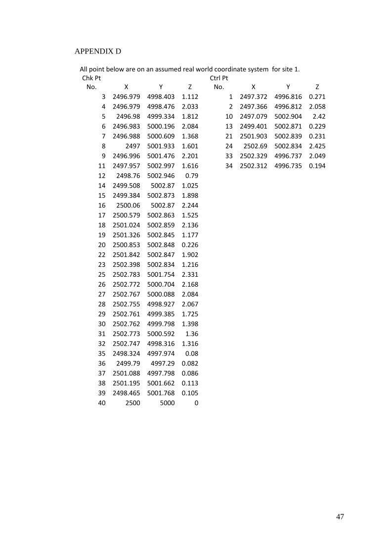
APPENDIX D
All point below are on an assumed real world coordinate system for site 1. Chk Pt
No. X Y Z Ctrl Pt
No. X Y Z
3 2496.979 4998.403 1.112 1 2497.372 4996.816 0.271
4 2496.979 4998.476 2.033 2 2497.366 4996.812 2.058
5 2496.98 4999.334 1.812 10 2497.079 5002.904 2.42
6 2496.983 5000.196 2.084 13 2499.401 5002.871 0.229
7 2496.988 5000.609 1.368 21 2501.903 5002.839 0.231
8 2497 5001.933 1.601 24 2502.69 5002.834 2.425
9 2496.996 5001.476 2.201 33 2502.329 4996.737 2.049
11 2497.957 5002.997 1.616 34 2502.312 4996.735 0.194
12 2498.76 5002.946 0.79 14 2499.508 5002.87 1.025 15 2499.384 5002.873 1.898 16 2500.06 5002.87 2.244 17 2500.579 5002.863 1.525 18 2501.024 5002.859 2.136 19 2501.326 5002.845 1.177 20 2500.853 5002.848 0.226 22 2501.842 5002.847 1.902 23 2502.398 5002.834 1.216 25 2502.783 5001.754 2.331 26 2502.772 5000.704 2.168 27 2502.767 5000.088 2.084 28 2502.755 4998.927 2.067 29 2502.761 4999.385 1.725 30 2502.762 4999.798 1.398 31 2502.773 5000.592 1.36 32 2502.747 4998.316 1.316 35 2498.324 4997.974 0.08 36 2499.79 4997.29 0.082 37 2501.088 4997.798 0.086 38 2501.195 5001.662 0.113 39 2498.465 5001.768 0.105 40 2500 5000 0

48
APPENDIX E
All point below are on an assumed real world coordinate system FOR SITE 2 Chk Pt
No. X Y Z Ctrl Pt
No. X Y Z
2 2506.543 5021.798 101.288 1 2506.613 5021.791 100.176
4 2507.778 5021.781 102.064 3 2506.459 5021.168 102.367
5 2507.816 5021.78 101.035 11 2509.734 5021.404 100.279
6 2508.475 5021.581 101.294 16 2509.304 5018.049 103.677
7 2509.503 5020.82 102.364 22 2508.995 5015.108 100.155
8 2509.775 5020.73 101.763 29 2508.791 5013.765 102.29
9 2509.74 5021.426 101.423 39 2514.905 5013.71 99.998
10 2508.843 5021.54 100.184 40 2516.128 5013.571 102.055
12 2509.635 5019.642 100.856 13 2509.56 5018.983 101.925 14 2509.321 5017.994 102.186 15 2509.48 5019.248 102.829 17 2509.065 5015.756 102.571 18 2509.332 5017.029 101.844 19 2509.296 5017.661 101.171 20 2509.374 5018.408 100.15 21 2509.26 5016.407 100.849 23 2508.966 5014.855 101.691 24 2509.304 5014.336 100.157 25 2509.676 5014.3 100.899 26 2510.361 5014.225 101.046 27 2509.223 5014.35 101.414 28 2509.76 5014.287 102.05 30 2511.331 5013.478 102.277 31 2513.3 5013.258 102.267 32 2514.832 5013.719 101.798 33 2513.946 5013.821 101.412 34 2511.56 5014.087 101.543 35 2512.81 5013.948 101.147 36 2514.968 5013.703 100.904 37 2511.832 5014.058 100.762 38 2511.947 5014.039 100.028

49
APPENDIX F
All point are on an assumed real world coordinate system FOR SITE 3 Chk Pt
No. X Y Z Ctrl Pt
No. X Y Z
10 2502.257 5021.374 100.09 1 2499.461 5020.228 100.496
11 2505.185 5020.091 100.046 2 2502.653 5019.768 100.613
12 2504.805 5018.335 100.076 3 2505.971 5019.21 100.7255
13 2501.506 5018.467 100.028 4 2505.152 5012.928 100.728
14 2500.016 5018.993 99.992 5 2502.173 5013.051 100.598
15 2500.568 5017.453 99.974 6 2498.981 5014.27 100.537
16 2503.252 5017.218 100.026 7 2497.887 5009.227 100.5715
17 2506.773 5016.979 100.215 8 2502.218 5007.688 100.687
18 2505.671 5015.882 100.128 9 2505.09 5008.746 100.805
19 2504.238 5016.228 100.056 20 2502.02 5016.389 99.9805 21 2499.533 5016.275 99.95 22 2499.892 5014.78 99.924 23 2501.804 5014.594 99.987 24 2502.867 5014.195 100.022 25 2504.832 5014.221 100.107 26 2503.661 5012.749 100.12 27 2501.942 5011.715 100.042 28 2500.63 5013.069 99.9765 29 2499.174 5012.733 99.911 30 2498.563 5011.55 99.9415 31 2500.631 5011.168 99.973 32 2504.035 5011.126 100.154 33 2505.56 5011.135 100.178 34 2504.389 5009.653 100.136 35 2503.073 5009.662 100.115 36 2499.431 5010.366 99.9655 37 2499.125 5008.439 99.9835 38 2501.632 5008.855 100.04 39 2503.573 5008.627 100.145 40 2503.117 5006.654 100.154 41 2501.169 5006.213 100.042 42 2498.305 5006.648 100.024

50
APPENDIX G
Using 8 control points Site 1 View 1
Program x Photo x Diff
Program y Photo y Diff
164.1246 155.491 8.63364
-756.0806 -757.202 1.121431
158.1498 153.127 5.02283
-456.1607 -454.933 -1.22774
256.7763 247.71 9.066254
-542.342 -539.944 -2.39765
331.7018 322.017 9.684814
-481.444 -479.256 -2.18813
373.0825 360.39 12.69247
-670.524 -670.078 -0.44595
459.1571 444.725 14.43207
-617.959 -614.295 -3.66393
425.3922 414.146 11.24617
-476.355 -473.545 -2.80964
707.5612 695.239 12.32217
-615.475 -612.315 -3.15959
872.9471 865.13 7.817092
-778.791 -779.194 0.403225
1021.6565 1018.311 3.34553
-729.186 -728.29 -0.89553
992.5652 988.461 4.104237
-552.251 -546.391 -5.86028
1128.4834 1129.379 -0.89564
-479.023 -471.51 -7.51306
1236.1621 1239.779 -3.61694
-623.891 -619.005 -4.88641
1324.5611 1330.636 -6.07494
-497.692 -491.739 -5.9533
1388.0384 1395.642 -7.60357
-691.647 -688.906 -2.74144
1295.2119 1301.205 -5.99312
-884.670 -887.119 2.449372
1490.7571 1500.548 -9.79092
-542.521 -539.028 -3.4927
1603.8812 1615.411 -11.5298
-679.757 -678.922 -0.83466
1740.9273 1748.295 -7.36768
-430.234 -429.071 -1.16312
1809.0493 1816.39 -7.34071
-445.956 -445.857 -0.0993
1856.5777 1862.695 -6.11728
-453.736 -453.569 -0.16718
1965.3752 1968.016 -2.64083
-428.628 -431.34 2.711833
1918.5452 1923.527 -4.98177
-539.491 -538.857 -0.6344
1879.4606 1887.711 -8.2504
-634.216 -634.786 0.569749
1816.9572 1824.609 -7.65185
-646.003 -644.313 -1.68962
2033.1348 2036.268 -3.1332
-655.191 -654.782 -0.40905
586.5156 580.988 5.527618
-1102.944 -1110.964 8.019777
1084.2186 1091.28 -7.06136
-1136.445 -1145.415 8.970447
1531.5957 1550.125 -18.5293
-1090.647 -1094.291 3.64376
1394.8727 1405.103 -10.2303
-932.285 -935.817 3.531604
789.2362 779.085 10.15123
-944.010 -949.872 5.861765
1138.7168 1142.518 -3.80125
-1016.995 -997.954 -19.0413

51
Using the 5 corner control points Site 1 View 1
Program x Photo x Diff
Program y Photo y Diff
162.1960 155.4910 6.7050
-758.2762 -757.2020 -1.0742
156.6510 153.1270 3.5240
-458.3780 -454.9330 -3.4450
253.7121 247.7100 6.0021
-545.5243 -539.9440 -5.5803
327.5722 322.0170 5.5552
-485.4477 -479.2560 -6.1917
368.2038 360.3900 7.8138
-674.8421 -670.0780 -4.7641
453.0577 444.7250 8.3327
-623.1605 -614.2950 -8.8655
419.8814 414.1460 5.7354
-481.3155 -473.5450 -7.7705
700.8590 695.2390 5.6200
-621.3007 -612.3150 -8.9857
866.2630 865.1300 1.1330
-784.5089 -779.1940 -5.3149
1014.9944 1018.3110 -3.3166
-734.8867 -728.2900 -6.5967
985.9472 988.4610 -2.5138
-558.1917 -546.3910 -11.8007
1121.6744 1129.3790 -7.7046
-485.1830 -471.5100 -13.6730
1229.1760 1239.7790 -10.6030
-629.7745 -619.0050 -10.7695
1317.2999 1330.6360 -13.3361
-503.9176 -491.7390 -12.1786
1380.7198 1395.6420 -14.9222
-697.3998 -688.9060 -8.4938
1288.2216 1301.2050 -12.9834
-890.1170 -887.1190 -2.9980
1482.9882 1500.5480 -17.5598
-548.6946 -539.0280 -9.6666
1595.8181 1615.4110 -19.5929
-685.5494 -678.9220 -6.6274
1732.7610 1748.2950 -15.5340
-436.4055 -429.0710 -7.3345
1801.5107 1816.3900 -14.8793
-451.4477 -445.8570 -5.5907
1849.4436 1862.6950 -13.2514
-458.7671 -453.5690 -5.1981
1959.0267 1968.0160 -8.9893
-432.8123 -431.3400 -1.4723
1912.0403 1923.5270 -11.4867
-543.5502 -538.8570 -4.6932
1872.8140 1887.7110 -14.8970
-638.2242 -634.7860 -3.4382
1809.7810 1824.6090 -14.8280
-650.5882 -644.3130 -6.2752
2027.6947 2036.2680 -8.5733
-657.5869 -654.7820 -2.8049
585.9854 580.9880 4.9974
-1104.6344 -1110.9640 6.3296
1085.3920 1091.2800 -5.8880
-1136.4861 -1145.4150 8.9289
1530.4221 1550.1250 -19.7029
-1091.1399 -1094.2910 3.1511
1388.6538 1405.1030 -16.4492
-936.9511 -935.8170 -1.1341
783.4459 779.0850 4.3609
-949.1013 -949.8720 0.7707
1134.8038 1142.5180 -7.7142
-1020.5152 -997.9540 -22.5612

52
Using 6 control points Site 1 View 2
Program x Photo x Diff
Program y Photo y Diff
455.711538 451.136 4.575538
-486.06612 -487.054 0.98788
567.879785 560.991 6.888785
-642.60508 -642.485 -0.12008
649.597707 645.285 4.312707
-513.38055 -510.423 -2.95755
713.123707 707.826 5.297707
-711.13201 -711.505 0.37299
631.649602 624.011 7.638602
-911.48717 -916.588 5.10083
800.083068 797.15 2.933068
-563.00504 -560.176 -2.82904
898.071983 897.283 0.788983
-696.55032 -695.96 -0.59032
1079.80807 1082.865 -3.05693
-469.39247 -464.322 -5.07047
1217.96168 1224.856 -6.89432
-492.31459 -486.719 -5.59559
1309.15562 1318.353 -9.19738
-504.72085 -500.459 -4.26185
1505.15621 1515.874 -10.7178
-495.63036 -492.28 -3.35036
1423.95671 1432.801 -8.84429
-584.39017 -579.37 -5.02017
1355.31268 1365.779 -10.4663
-663.00521 -661.121 -1.88421
1235.97841 1242.576 -6.59759
-670.37389 -669.001 -1.37289
1622.63902 1633.354 -10.715
-686.80371 -684.214 -2.58971
609.468644 602.677 6.7916
-1210.4258 -1216.493 6.0672
1207.56948 1208.843 -1.2735
-1168.6215 -1174.712 6.0905
1410.57135 1418.506 -7.9347
-1080.6882 -1085.618 4.9298
821.340856 816.576 4.7649
-952.15310 -957.89 5.7369
777.713644 771.813 5.9006
-1057.9919 -1038.587 -19.4049
Using 6 control points Site 1 View 3
Program x Photo x Diff
Program y Photo y Diff
545.3301 532.547 12.78307
-752.6593 -753.02 0.360704
549.4704 541.022 8.44844
-490.2493 -487.073 -3.1763
726.9034 717.648 9.255374
-553.561 -549.966 -3.59536
876.0001 871.261 4.739148
-486.753 -482.425 -4.32843
946.7425 942.02 4.722516
-658.510 -656.668 -1.84205
1128.9256 1129.127 -0.20142
-598.984 -594.184 -4.79996
1066.6199 1065.427 1.19289
-466.955 -461.858 -5.09654
1418.6733 1425.034 -6.36073
-589.975 -587.933 -2.04249
1566.7870 1577.151 -10.364
-766.100 -767.814 1.71381
1714.0950 1722.631 -8.53602
-718.975 -722.052 3.076884
1689.0085 1698.176 -9.16745
-521.249 -522.839 1.590134
1839.9310 1844.948 -5.01696
-433.956 -437.801 3.844889
743.1496 737.69 5.459561
-1102.340 -1110.795 8.454583
966.7774 968.048 -1.27056
-1213.327 -1222.067 8.740348
1520.9411 1535.545 -14.6039
-1237.712 -1243.236 5.523588
1386.6849 1393.276 -6.5911
-940.307 -945.196 4.88922
1523.3863 1533.949 -10.5627
-1069.173 -1046.456 -22.7173
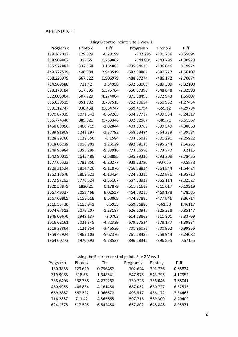
53
APPENDIX H
Using 8 control points Site 2 View 1
Program x Photo x Diff
Program y Photo y Diff
129.347013 129.629 -0.28199
-702.295 -701.736 -0.55894
318.909862 318.65 0.259862
-544.804 -543.795 -1.00928
335.522883 332.368 3.154883
-735.84626 -736.046 0.19974
449.777519 446.834 2.943519
-682.38807 -680.727 -1.66107
668.228979 667.322 0.906979
-488.87274 -486.172 -2.70074
714.969580 711.42 3.54958
-592.63008 -589.309 -3.32108
623.170784 617.595 5.575784
-650.87398 -648.848 -2.02598
512.003064 507.729 4.274064
-871.38493 -872.943 1.55807
855.639515 851.902 3.737515
-752.20654 -750.932 -1.27454
939.312747 938.458 0.854747
-559.41794 -555.12 -4.29794
1070.87035 1071.543 -0.67265
-504.77717 -499.534 -5.24317
885.774346 885.021 0.753346
-392.32567 -385.71 -6.61567
1458.89056 1460.719 -1.82844
-403.93768 -399.549 -4.38868
1239.91908 1241.297 -1.37792
-568.63484 -564.239 -4.39584
1128.39760 1128.556 -0.1584
-703.55022 -701.291 -2.25922
1018.06239 1016.801 1.26139
-892.68135 -895.244 2.56265
1349.95984 1355.299 -5.33916
-773.16550 -773.377 0.2115
1642.90015 1645.489 -2.58885
-595.99336 -593.209 -2.78436
1777.65323 1783.856 -6.20277
-938.23780 -937.65 -0.5878
1809.31524 1814.426 -5.11076
-766.38824 -764.844 -1.54424
1862.18676 1868.321 -6.13424
-724.83313 -722.876 -1.95713
1772.97293 1776.524 -3.55107
-657.13927 -655.114 -2.02527
1820.38879 1820.21 0.17879
-511.81619 -511.617 -0.19919
2067.49337 2059.468 8.02537
-464.39215 -469.178 4.78585
2167.09869 2158.518 8.58069
-474.97886 -477.846 2.86714
2116.53430 2115.941 0.5933
-559.86883 -561.33 1.46117
2074.67513 2076.207 -1.53187
-626.10947 -625.258 -0.85147
1946.06670 1949.137 -3.0703
-614.13869 -611.801 -2.33769
2016.62161 2021.345 -4.72339
-679.57534 -678.177 -1.39834
2118.38864 2121.854 -3.46536
-701.96056 -700.962 -0.99856
1959.42924 1965.103 -5.67376
-761.18482 -758.944 -2.24082
1964.60773 1970.393 -5.78527
-896.18345 -896.855 0.67155
Using the 5 corner control points Site 2 View 1
Program x Photo x Diff
Program y Photo y Diff
130.3855 129.629 0.756482
-702.624 -701.736 -0.88824
319.9985 318.65 1.348541
-547.975 -543.795 -4.17952
336.6403 332.368 4.272262
-739.726 -736.046 -3.68041
450.9955 446.834 4.161454
-687.052 -680.727 -6.32516
669.2887 667.322 1.966672
-493.517 -486.172 -7.34463
716.2857 711.42 4.865665
-597.713 -589.309 -8.40409
624.1375 617.595 6.542458
-657.802 -648.848 -8.95371

54
513.5142 507.729 5.78525
-877.726 -872.943 -4.78292
858.5971 851.902 6.695063
-754.382 -750.932 -3.44957
941.9471 938.458 3.489149
-558.932 -555.12 -3.8115
1074.151 1071.543 2.607825
-500.343 -499.534 -0.80869
887.4603 885.021 2.439255
-392.506 -385.71 -6.79583
1463.299 1460.719 2.580333
-390.108 -399.549 9.44142
1244.419 1241.297 3.12242
-560.866 -564.239 3.372727
1133.308 1128.556 4.752203
-698.244 -701.291 3.046767
1023.268 1016.801 6.466739
-891.117 -895.244 4.127364
1356.861 1355.299 1.561806
-763.381 -773.377 9.995753
1650.202 1645.489 4.712961
-577.745 -593.209 15.46422
1789.116 1783.856 5.25961
-920.813 -937.65 16.83691
1818.136 1814.426 3.709661
-749.506 -764.844 15.33753
1869.545 1868.321 1.224434
-710.466 -722.876 12.40982
1781.103 1776.524 4.579475
-637.938 -655.114 17.17643
1825.884 1820.21 5.674154
-494.719 -511.617 16.8981
2070.239 2059.468 10.77053
-450.824 -469.178 18.35445
2167.405 2158.518 8.887133
-467.687 -477.846 10.15874
2116.525 2115.941 0.583689
-558.095 -561.33 3.234975
2076.531 2076.207 0.323998
-622.265 -625.258 2.992882
1950.401 1949.137 1.2642
-603.673 -611.801 8.127753
2020.438 2021.345 -0.90727
-672.87 -678.177 5.307405
2120.449 2121.854 -1.40477
-700.445 -700.962 0.516583
1965.482 1965.103 0.378646
-751.86 -758.944 7.08412
1972.428 1970.393 2.034544
-887.761 -896.855 9.094314
Using 8 control points Site 2 View 2
Program x Photo x Diff
Program y Photo y Diff
65.9300 57.819 8.110985
-654.4277 -652.213 -2.21469
261.9210 251.647 10.27404
-536.1778 -531.546 -4.63176
272.4084 258.697 13.71141
-691.903 -692.033 0.129819
379.6042 368.438 11.16615
-652.939 -651.282 -1.65683
565.5847 562.84 2.74468
-493.414 -488.061 -5.35254
610.6601 606.24 4.420105
-584.058 -580.284 -3.77394
566.3444 556.409 9.935392
-634.134 -631.769 -2.36452
438.9985 425.933 13.06545
-815.072 -821.138 6.066187
661.5587 661.778 -0.21928
-724.357 -723.977 -0.37982
693.2872 698.214 -4.92677
-553.329 -551.225 -2.1044
729.3464 739.159 -9.81259
-502.473 -501.242 -1.23072
660.6617 666.158 -5.49634
-405.925 -400.844 -5.08135
885.0664 894.082 -9.01562
-402.881 -412.789 9.907811
811.6062 820.511 -8.90479
-559.271 -558.475 -0.79576
753.8147 761.928 -8.1133
-681.780 -677.382 -4.39777
710.4666 714.258 -3.79139
-851.300 -848.747 -2.5527
857.4603 865.005 -7.5447
-748.592 -740.691 -7.90126

55
965.1632 966.847 -1.68378
-581.380 -581.082 -0.29811
1089.2498 1082.736 6.51384
-919.527 -892.538 -26.9891
1160.5304 1149.818 10.71245
-754.928 -741.373 -13.5551
1286.5945 1270.924 15.67049
-720.669 -709.856 -10.8134
1073.1784 1066.766 6.412373
-642.690 -636.972 -5.71827
1178.1885 1165.335 12.85352
-503.298 -510.029 6.731481
1551.2977 1513.786 37.51171
-458.567 -468.468 9.900771
1858.9124 1823.882 35.03041
-475.198 -480.38 5.182311
1962.6483 1957.494 5.154293
-574.402 -572.759 -1.64302
1844.3976 1832.485 11.91263
-643.317 -639.286 -4.03118
1492.6739 1470.385 22.28886
-616.751 -613.646 -3.1048
1683.5745 1666.322 17.25249
-694.097 -688.688 -5.40942
1974.1686 1974.284 -0.11536
-733.103 -728.87 -4.23313
1533.1516 1513.801 19.35065
-772.430 -761.653 -10.7767
1549.2521 1530.718 18.53407
-915.65 -900.295 -15.355
Using the 5 corner control points
Program x Photo x Diff
Program y Photo y Diff
130.3855 129.629 0.756482
-702.624 -701.736 -0.88824
319.9985 318.65 1.348541
-547.975 -543.795 -4.17952
336.6403 332.368 4.272262
-739.726 -736.046 -3.68041
450.9955 446.834 4.161454
-687.052 -680.727 -6.32516
669.2887 667.322 1.966672
-493.517 -486.172 -7.34463
716.2857 711.42 4.865665
-597.713 -589.309 -8.40409
624.1375 617.595 6.542458
-657.802 -648.848 -8.95371
513.5142 507.729 5.78525
-877.726 -872.943 -4.78292
858.5971 851.902 6.695063
-754.382 -750.932 -3.44957
941.9471 938.458 3.489149
-558.932 -555.12 -3.8115
1074.151 1071.543 2.607825
-500.343 -499.534 -0.80869
887.4603 885.021 2.439255
-392.506 -385.71 -6.79583
1463.299 1460.719 2.580333
-390.108 -399.549 9.44142
1244.419 1241.297 3.12242
-560.866 -564.239 3.372727
1133.308 1128.556 4.752203
-698.244 -701.291 3.046767
1023.268 1016.801 6.466739
-891.117 -895.244 4.127364
1356.861 1355.299 1.561806
-763.381 -773.377 9.995753
1650.202 1645.489 4.712961
-577.745 -593.209 15.46422
1789.116 1783.856 5.25961
-920.813 -937.65 16.83691
1818.136 1814.426 3.709661
-749.506 -764.844 15.33753
1869.545 1868.321 1.224434
-710.466 -722.876 12.40982
1781.103 1776.524 4.579475
-637.938 -655.114 17.17643
1825.884 1820.21 5.674154
-494.719 -511.617 16.8981
2070.239 2059.468 10.77053
-450.824 -469.178 18.35445
2167.405 2158.518 8.887133
-467.687 -477.846 10.15874
2116.525 2115.941 0.583689
-558.095 -561.33 3.234975
2076.531 2076.207 0.323998
-622.265 -625.258 2.992882

56
1950.401 1949.137 1.2642
-603.673 -611.801 8.127753
2020.438 2021.345 -0.90727
-672.87 -678.177 5.307405
2120.449 2121.854 -1.40477
-700.445 -700.962 0.516583
1965.482 1965.103 0.378646
-751.86 -758.944 7.08412
1972.428 1970.393 2.034544
-887.761 -896.855 9.094314
Using 8 control points Site 2 View 3
Program x Photo x Diff
Program y Photo y Diff
64.4361 67.175 -2.7389
-736.649 -736.054 -0.59503
275.9028 276.114 -0.21117
-608.5605 -607.063 -1.49748
283.7443 281.531 2.213252
-778.733 -778.842 0.108957
400.5742 398.219 2.355242
-736.733 -735.823 -0.9097
610.1245 608.786 1.338519
-566.584 -564.141 -2.44293
656.0158 652.641 3.374817
-664.266 -662.103 -2.16288
595.2610 590.743 4.518031
-717.538 -715.577 -1.96081
459.8183 456.22 3.598324
-912.976 -914.956 1.980467
731.4842 725.827 5.657234
-815.466 -816.098 0.631537
783.7814 780.641 3.140381
-632.233 -629.621 -2.6123
850.9427 847.481 3.461715
-578.078 -573.6 -4.47809
746.3414 744.1 2.241371
-474.132 -467.185 -6.94701
1092.5246 1090.548 1.976583
-473.035 -467.335 -5.70045
964.5531 961.248 3.305081
-639.861 -637.429 -2.4324
883.4647 878.885 4.5797
-770.883 -770.178 -0.70472
813.5117 808.11 5.401745
-953.224 -957.644 4.419622
1030.9953 1028.313 2.682334
-843.822 -846.162 2.339757
1212.2063 1210.179 2.027259
-665.255 -662.536 -2.7186
1350.5432 1354.883 -4.33982
-1029.788 -1035.276 5.487888
1418.3327 1424.555 -6.22228
-852.334 -853.981 1.647146
1533.2658 1542.814 -9.54823
-815.654 -816.004 0.350118
1339.5523 1341.78 -2.22769
-732.040 -730.99 -1.04971
1438.1937 1442.539 -4.34527
-584.369 -582.666 -1.7028
1807.6329 1810.508 -2.87513
-542.982 -543.849 0.867262
2066.6716 2064.538 2.133619
-565.106 -566.286 1.180462
2117.7423 2119.107 -1.36467
-667.183 -667.498 0.3155
2018.8957 2024.392 -5.49631
-736.399 -735.269 -1.12955
1717.7640 1727.039 -9.27502
-707.049 -705.88 -1.16852
1882.3399 1891.678 -9.33815
-788.044 -787.472 -0.57151
2126.5330 2130.203 -3.67
-827.973 -826.957 -1.01593
1751.5712 1761.972 -10.4008
-869.562 -869.373 -0.18898
1764.6034 1775.939 -11.3356
-1019.188 -1020.763 1.575316

57
Using the 5 corner control points
Program x Photo x Diff
Program y Photo y Diff
63.61048 57.819 5.791482
-656.692 -652.213 -4.4794
261.9677 251.647 10.32066
-541.927 -531.546 -10.3812
270.2867 258.697 11.58968
-698.4 -692.033 -6.36723
378.6103 368.438 10.17229
-660.474 -651.282 -9.19174
567.7885 562.84 4.948522
-501.119 -488.061 -13.0581
612.0218 606.24 5.781809
-592.256 -580.284 -11.9718
565.6903 556.409 9.281324
-644.7 -631.769 -12.9307
436.2068 425.933 10.27379
-824.558 -821.138 -3.41993
664.4301 661.778 2.652128
-728.412 -723.977 -4.43548
699.4108 698.214 1.196846
-553.989 -551.225 -2.76407
738.9634 739.159 -0.19559
-497.695 -501.242 3.546529
667.4289 666.158 1.270931
-407.728 -400.844 -6.8838
903.3275 894.082 9.245487
-384.397 -412.789 28.3924
823.8323 820.511 3.321293
-549.476 -558.475 8.999082
763.1436 761.928 1.215555
-675.399 -677.382 1.982605
716.0153 714.258 1.757337
-849.919 -848.747 -1.17228
870.8165 865.005 5.811531
-735.329 -740.691 5.362274
986.4514 966.847 19.60436
-555.493 -581.082 25.58922
1110.86 1082.736 28.12369
-893.214 -892.538 -0.6762
1181.775 1149.818 31.95671
-729.474 -741.373 11.89853
1306.196 1270.924 35.27184
-698.551 -709.856 11.30489
1095.795 1066.766 29.02946
-614.518 -636.972 22.45361
1199.682 1165.335 34.34677
-478.187 -510.029 31.8417
1569.582 1513.786 55.79614
-437.445 -468.468 31.02321
1869.714 1823.882 45.83168
-463.383 -480.38 16.99653
1968.006 1957.494 10.51222
-571.213 -572.759 1.545519
1853.218 1832.485 20.73266
-636.52 -639.286 2.766444
1508.76 1470.385 38.37502
-600.268 -613.646 13.37808
1696.228 1666.322 29.90595
-682.762 -688.688 5.92609
1980.696 1974.284 6.412134
-729.547 -728.87 -0.67709
1548.954 1513.801 35.15255
-757.062 -761.653 4.591196
1565.299 1530.718 34.58089
-901.217 -900.295 -0.92157

58
APPENDIX I
Using 9 control points Site 3 View 1
Program x Photo x Diff
Program y Photo y Diff
1496.72 1502.09 -5.37001
-788.96 -789.508 0.547535
1851.237 1856.543 -5.30608
-823.026 -828.371 5.344665
1822.665 1829.158 -6.49288
-848.383 -849.818 1.435385
1383.848 1388.697 -4.84884
-838.114 -838.562 0.44753
1206.145 1206.895 -0.75047
-827.658 -828.251 0.59288
1246.206 1248.383 -2.17743
-859.928 -861.311 1.382594
1612.294 1621.336 -9.042
-870.336 -871.962 1.625913
2141.141 2134.629 6.512154
-866.164 -867.002 0.838254
1996.235 1996.751 -0.51589
-899.052 -901.223 2.170533
1763.126 1771.734 -8.60839
-893.278 -895.677 2.398508
1431.728 1439.194 -7.46588
-888.632 -890.6 1.968211
1077.709 1075.599 2.1098
-882.76 -884.551 1.790735
1083.266 1080.593 2.672877
-924.861 -927.483 2.62249
1377.225 1383.443 -6.21808
-932.005 -934.817 2.811663
1549.081 1557.974 -8.8928
-944.985 -946.998 2.012632
1890.874 1897.414 -6.54032
-943.49 -944.674 1.183582
1694.937 1703.28 -8.34328
-982.16 -984.109 1.949313
1353.483 1361.07 -7.58671
-1022.72 -1026.98 4.263768
1147.187 1148.8 -1.61294
-972.735 -976.452 3.717214
884.4883 879.444 5.044274
-984.533 -987.437 2.904126
707.4581 698.79 8.668148
-1018.19 -1021.283 3.095497
1077.106 1078.858 -1.75195
-1047.5 -1051.717 4.214534
1790.988 1796.625 -5.63748
-1046.93 -1047.204 0.278304
2138.25 2129.238 9.011925
-1057.43 -1054.254 -3.17337
1909.714 1912.1 -2.38621
-1136.8 -1135.301 -1.50059
1577.594 1586.828 -9.23421
-1123.66 -1125.445 1.789911
791.7378 786.783 4.954809
-1074.69 -1078.977 4.290249
558.7164 555.669 3.047401
-1180.21 -1182.719 2.506413
1202.107 1209.046 -6.93879
-1174.33 -1178.658 4.324969
1713.419 1720.769 -7.35036
-1194.32 -1193.349 -0.97313
1583.877 1593.074 -9.1972
-1372.73 -1368.775 -3.95326
897.5252 905.728 -8.2028
-1414.2 -1415.488 1.289615
95.7755 105.03 -9.2545
-1304.02 -1299.956 -4.06007
Using the 4 corner control points Site 3 View 1
Program x Photo x Diff
Program y Photo y Diff
1497.215 1502.09 -4.87522
-789.187 -789.508 0.321187
1851.544 1856.543 -4.9994
-822.805 -828.371 5.565537
1822.168 1829.158 -6.98964
-848.016 -849.818 1.801716
1383.196 1388.697 -5.50137
-838.175 -838.562 0.386891
1205.789 1206.895 -1.10625
-827.947 -828.251 0.303782
1245.125 1248.383 -3.2582
-860 -861.311 1.310871
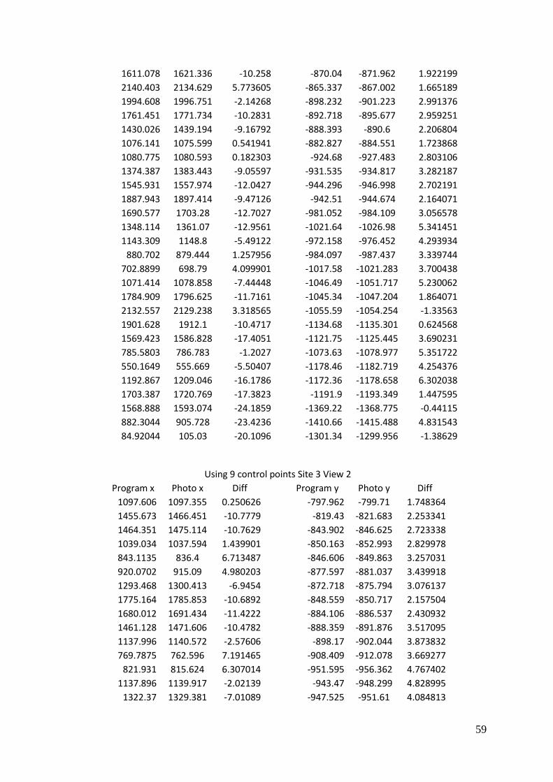
59
1611.078 1621.336 -10.258
-870.04 -871.962 1.922199
2140.403 2134.629 5.773605
-865.337 -867.002 1.665189
1994.608 1996.751 -2.14268
-898.232 -901.223 2.991376
1761.451 1771.734 -10.2831
-892.718 -895.677 2.959251
1430.026 1439.194 -9.16792
-888.393 -890.6 2.206804
1076.141 1075.599 0.541941
-882.827 -884.551 1.723868
1080.775 1080.593 0.182303
-924.68 -927.483 2.803106
1374.387 1383.443 -9.05597
-931.535 -934.817 3.282187
1545.931 1557.974 -12.0427
-944.296 -946.998 2.702191
1887.943 1897.414 -9.47126
-942.51 -944.674 2.164071
1690.577 1703.28 -12.7027
-981.052 -984.109 3.056578
1348.114 1361.07 -12.9561
-1021.64 -1026.98 5.341451
1143.309 1148.8 -5.49122
-972.158 -976.452 4.293934
880.702 879.444 1.257956
-984.097 -987.437 3.339744
702.8899 698.79 4.099901
-1017.58 -1021.283 3.700438
1071.414 1078.858 -7.44448
-1046.49 -1051.717 5.230062
1784.909 1796.625 -11.7161
-1045.34 -1047.204 1.864071
2132.557 2129.238 3.318565
-1055.59 -1054.254 -1.33563
1901.628 1912.1 -10.4717
-1134.68 -1135.301 0.624568
1569.423 1586.828 -17.4051
-1121.75 -1125.445 3.690231
785.5803 786.783 -1.2027
-1073.63 -1078.977 5.351722
550.1649 555.669 -5.50407
-1178.46 -1182.719 4.254376
1192.867 1209.046 -16.1786
-1172.36 -1178.658 6.302038
1703.387 1720.769 -17.3823
-1191.9 -1193.349 1.447595
1568.888 1593.074 -24.1859
-1369.22 -1368.775 -0.44115
882.3044 905.728 -23.4236
-1410.66 -1415.488 4.831543
84.92044 105.03 -20.1096
-1301.34 -1299.956 -1.38629
Using 9 control points Site 3 View 2
Program x Photo x Diff
Program y Photo y Diff
1097.606 1097.355 0.250626
-797.962 -799.71 1.748364
1455.673 1466.451 -10.7779
-819.43 -821.683 2.253341
1464.351 1475.114 -10.7629
-843.902 -846.625 2.723338
1039.034 1037.594 1.439901
-850.163 -852.993 2.829978
843.1135 836.4 6.713487
-846.606 -849.863 3.257031
920.0702 915.09 4.980203
-877.597 -881.037 3.439918
1293.468 1300.413 -6.9454
-872.718 -875.794 3.076137
1775.164 1785.853 -10.6892
-848.559 -850.717 2.157504
1680.012 1691.434 -11.4222
-884.106 -886.537 2.430932
1461.128 1471.606 -10.4782
-888.359 -891.876 3.517095
1137.996 1140.572 -2.57606
-898.17 -902.044 3.873832
769.7875 762.596 7.191465
-908.409 -912.078 3.669277
821.931 815.624 6.307014
-951.595 -956.362 4.767402
1137.896 1139.917 -2.02139
-943.47 -948.299 4.828995
1322.37 1329.381 -7.01089
-947.525 -951.61 4.084813

60
1639.67 1649.987 -10.3168
-929.604 -933.006 3.401685
1518.653 1527.95 -9.29708
-975.344 -979.726 4.381614
1235.665 1239.101 -3.43609
-1034.58 -1040.39 5.809521
956.1844 953.233 2.951419
-996.891 -1002.18 5.289601
679.0334 670.758 8.275389
-1025.59 -1030.29 4.698528
529.7041 522.39 7.314136
-1073.62 -1077.96 4.335886
975.0133 974.364 0.649336
-1078.24 -1084.51 6.267535
1688.416 1695.55 -7.13425
-1031.21 -1033.35 2.142347
1991.255 1990.631 0.623665
-1021.25 -1022.18 0.931929
1890.622 1893.031 -2.4085
-1108.14 -1108.67 0.529793
1585.226 1593.282 -8.05639
-1118.49 -1121.51 3.021355
702.3647 699.708 2.656749
-1128.17 -1134.17 6.003973
579.7674 578.877 0.890363
-1264.65 -1268.69 4.038265
1275.679 1280.66 -4.98111
-1198.41 -1203.72 5.313229
1799.045 1801.386 -2.34079
-1176.31 -1175.56 -0.75536
1912.802 1904.642 8.160049
-1359.96 -1350.25 -9.71642
1278.441 1283.417 -4.97634
-1481.04 -1477.67 -3.36982
193.9729 208.271 -14.2981
-1462.93 -1454.84 -8.08864
Using the 4 corner control points Site 3 View 2
Program x Photo x Diff
Program y Photo y Diff
1099.286 1097.355 1.930589
-797.348 -799.71 2.3621
1456.374 1466.451 -10.0774
-818.487 -821.683 3.195846
1464.308 1475.114 -10.8057
-842.925 -846.625 3.699643
1039.849 1037.594 2.255034
-849.502 -852.993 3.490809
844.6813 836.4 8.281267
-846.102 -849.863 3.761053
920.8091 915.09 5.719092
-876.955 -881.037 4.081692
1293.169 1300.413 -7.24444
-871.817 -875.794 3.977157
1774.156 1785.853 -11.6969
-847.348 -850.717 3.369375
1678.413 1691.434 -13.0213
-882.907 -886.537 3.630265
1460.011 1471.606 -11.5955
-887.305 -891.876 4.571324
1137.629 1140.572 -2.94333
-897.317 -902.044 4.72665
770.513 762.596 7.916956
-907.778 -912.078 4.300076
821.6959 815.624 6.071851
-950.771 -956.362 5.590841
1136.486 1139.917 -3.43108
-942.478 -948.299 5.820603
1320.205 1329.381 -9.17602
-946.404 -951.61 5.206204
1636.937 1649.987 -13.0498
-928.332 -933.006 4.673846
1514.84 1527.95 -13.11
-974.006 -979.726 5.720264
1231.582 1239.101 -7.51897
-1033.15 -1040.386 7.23577
954.2984 953.233 1.065388
-995.795 -1002.181 6.386406
678.0896 670.758 7.331602
-1024.51 -1030.289 5.783061
528.5995 522.39 6.20951
-1072.32 -1077.958 5.635039
971.3518 974.364 -3.01222
-1076.72 -1084.511 7.791855
1682.461 1695.55 -13.089
-1029.55 -1033.348 3.795493
1984.887 1990.631 -5.74445
-1019.48 -1022.182 2.70156
1882.054 1893.031 -10.9769
-1106.03 -1108.666 2.632728
1577.368 1593.282 -15.914
-1116.45 -1121.507 5.061152

61
699.1616 699.708 -0.54638
-1126.44 -1134.174 7.738678
574.7614 578.877 -4.11564
-1261.83 -1268.688 6.862154
1267.523 1280.66 -13.1367
-1195.97 -1203.721 7.752798
1788.625 1801.386 -12.7614
-1173.84 -1175.559 1.722796
1896.357 1904.642 -8.28479
-1355.99 -1350.245 -5.74707
1263.474 1283.417 -19.9434
-1475.88 -1477.674 1.795974
188.7999 208.271 -19.4711
-1457.83 -1454.843 -2.98816
Using 9 control points Site 3 View 3
Program x Photo x Diff
Program y Photo y Diff
633.5281 627.498 6.030067
-712.153 -714.008 1.854906
1024.346 1028.198 -3.85225
-708.684 -708.755 0.070875
1074.136 1080.508 -6.37185
-732.055 -733.413 1.357543
640.2043 633.79 6.414296
-771.601 -774.432 2.831393
408.0448 400.669 7.375774
-784.677 -788.237 3.559645
540.4088 533.15 7.25877
-811.342 -814.999 3.657462
939.7998 940.697 -0.8972
-774.14 -776.434 2.294179
1392.482 1408.486 -16.0037
-714.19 -714.991 0.800641
1343.67 1356.197 -12.5273
-755.129 -756.664 1.535182
1133.115 1140.578 -7.46334
-776.303 -778.452 2.148573
809.4007 806.459 2.94175
-813.555 -817.343 3.78806
410.7316 403.218 7.513591
-859.286 -864.409 5.122924
532.0682 525.827 6.24121
-901.403 -906.277 4.874082
878.8748 877.515 1.35983
-860.596 -865.429 4.83347
1079.334 1083.013 -3.6789
-847.409 -851.599 4.189829
1370.3 1383.077 -12.7772
-802.084 -804.77 2.685677
1332.033 1342.13 -10.0966
-856.843 -861.17 4.326834
1130.472 1133.992 -3.51969
-944.616 -950.614 5.997608
764.8441 759.419 5.425089
-935.635 -941.461 5.826268
477.5599 471.665 5.89492
-999.915 -1004.768 4.853164
383.8143 379.449 4.365298
-1074.12 -1077.88 3.75749
909.5089 907.916 1.59293
-1020.7 -1027.007 6.303205
1577.173 1589.304 -12.1314
-895.448 -899.026 3.578459
1820.819 1832.118 -11.2994
-859.063 -861.735 2.671598
1853.885 1860.748 -6.86341
-949.384 -951.852 2.468126
1606.047 1613.998 -7.95089
-990.864 -995.306 4.441781
684.728 680.525 4.202956
-1111.6 -1116.105 4.50452
772.8467 770.497 2.349661
-1286.2 -1287.754 1.557486
1418.545 1422.437 -3.89153
-1108.47 -1112.375 3.905406
1883.666 1884.126 -0.45978
-1023.31 -1024.031 0.722627
2249.296 2218.716 30.57979
-1184.04 -1173.185 -10.8582
1856.234 1836.391 19.84348
-1400.73 -1387.095 -13.6364
670.4379 671.268 -0.83006
-1603.82 -1585.63 -18.1889

62
Using the 4 corner control points Site 3 View 3
Program x Photo x Diff
Program y Photo y Diff
633.6159 627.498 6.11794
-711.21 -714.008 2.797829
1023.812 1028.198 -4.38603
-707.919 -708.755 0.836239
1073.429 1080.508 -7.07852
-731.393 -733.413 2.020087
640.2318 633.79 6.441765
-770.766 -774.432 3.665711
408.5208 400.669 7.851837
-783.724 -788.237 4.512824
540.6159 533.15 7.465932
-810.492 -814.999 4.506606
939.2371 940.697 -1.45989
-773.469 -776.434 2.96531
1391.205 1408.486 -17.2806
-713.734 -714.991 1.256992
1342.327 1356.197 -13.8702
-754.695 -756.664 1.969396
1132.145 1140.578 -8.43344
-775.757 -778.452 2.694878
809.0321 806.459 2.573126
-812.855 -817.343 4.487809
411.2271 403.218 8.009123
-858.413 -864.409 5.996071
532.2669 525.827 6.439908
-900.608 -906.277 5.668836
878.2491 877.515 0.73414
-859.992 -865.429 5.437103
1078.246 1083.013 -4.76702
-846.919 -851.599 4.679529
1368.672 1383.077 -14.4047
-801.741 -804.77 3.028612
1330.207 1342.13 -11.9226
-856.56 -861.17 4.610309
1128.887 1133.992 -5.10458
-944.216 -950.614 6.398098
764.3773 759.419 4.958286
-935.002 -941.461 6.458973
477.8981 471.665 6.23309
-999.076 -1004.768 5.691593
384.4851 379.449 5.036135
-1073.18 -1077.88 4.703566
908.4296 907.916 0.513553
-1020.11 -1027.007 6.897114
1574.416 1589.304 -14.8878
-895.347 -899.026 3.679318
1817.612 1832.118 -14.5063
-859.082 -861.735 2.652502
1849.914 1860.748 -10.8338
-949.426 -951.852 2.425744
1602.625 1613.998 -11.3733
-990.746 -995.306 4.559811
684.2884 680.525 3.763443
-1110.76 -1116.105 5.344783
771.7808 770.497 1.283782
-1284.91 -1287.754 2.84556
1415.217 1422.437 -7.21965
-1108.06 -1112.375 4.319887
1878.966 1884.126 -5.1603
-1023.33 -1024.031 0.701551
2241.524 2218.716 22.80765
-1183.94 -1173.185 -10.7518
1848.865 1836.391 12.47354
-1399.48 -1387.095 -12.3849
669.5112 671.268 -1.75684
-1600.68 -1585.63 -15.0497
Using 8 control points Site 3 View 4
Program x Photo x Diff
Program y Photo y Diff
1042.088 1050.835 -8.74662
-1415.57 -1446.582 31.011
2018.474 2026.685 -8.21063
-1192.62 -1214.172 21.55318
1951.851 1965.824 -13.9731
-1071.64 -1096.993 25.34897
1300.311 1314.648 -14.3368
-1173.19 -1205.337 32.15122
26.07008 32.466 -6.39592
-1334.45 -1356.343 21.89082
375.5607 373.806 1.75472
-1151.93 -1179.537 27.60291
864.0314 864.5 -0.46858
-1126.44 -1157.931 31.49564

63
1441.731 1458.631 -16.9
-1055.22 -1085.339 30.11958
1888.01 1904.391 -16.3814
-964.107 -990.924 26.81695
1578.534 1598.78 -20.2464
-906.542 -934.772 28.22973
1212.748 1224.575 -11.8275
-937.351 -967.164 29.81328
947.5086 950.597 -3.08837
-940.917 -969.964 29.04686
482.0861 477.083 5.003142
-988.043 -1016.186 28.14349
638.7531 634.666 4.087122
-871.941 -898.661 26.72035
881.9421 883.626 -1.68387
-810.444 -836.728 26.2836
1236.72 1249.48 -12.7596
-843.831 -870.836 27.00505
1420.864 1438.317 -17.453
-815.601 -842.002 26.401
1376.596 1394.127 -17.5312
-765.752 -790.879 25.12749
1046.863 1053.346 -6.48279
-782.491 -807.721 25.22985
447.54 441.677 5.863003
-809.867 -834.718 24.85137
118.904 114.432 4.472028
-838.01 -862.702 24.692
300.7378 293.596 7.141794
-772.13 -797.344 25.21448
540.1081 534.036 6.072083
-754.701 -779.033 24.33189
1148.995 1158.918 -9.92337
-744.356 -768.472 24.11635
1037.056 1042.843 -5.78681
-696.055 -719.351 23.29563
722.698 719.356 3.342034
-726.211 -749.809 23.59833
399.7139 392.932 6.781948
-730.007 -753.46 23.45316
385.3098 379.081 6.228798
-679.77 -702.671 22.90066
639.9659 634.663 5.302869
-667.931 -690.626 22.69536
1013.461 1019.148 -5.6869
-651.682 -673.562 21.88014