Professional Forecasts of Interest Rates and Exchange Rates: Evidence from the Wall Street Journal’s Panel of Economists

Karlyn Mitchell

Department of Business Management North Carolina State University

Douglas K. Pearce*

Department of Economics North Carolina State University

March 2005

Abstract

We use individual economists’ 6-month-ahead forecasts of interest rates and exchange

rates from the Wall Street Journal’s survey to test for forecast unbiasedness, accuracy, and

heterogeneity. We find that a majority of economists produced unbiased forecasts but that none

predicted directions of changes more accurately than chance. We find that the forecast accuracy

of most of the economists is statistically indistinguishable from that of the random walk model

when forecasting the Treasury bill rate but that the forecast accuracy is significantly worse for

many of the forecasters for predictions of the Treasury bond rate and the exchange rate.

Regressions involving deviations in economists’ forecasts from forecast averages produced

evidence of systematic heterogeneity across economists, including evidence that independent

economists make more radical forecasts.

JEL code: E47

Keywords: Forecast evaluation, interest rates, exchange rate

* Corresponding author: Douglas K. Pearce, Department of Economics, North Carolina State

University, Raleigh, NC 27695-8110, phone: 919-513-2880, e-mail: Doug Pearce@ncsu.edu

1

Professional Forecasts of Interest Rates and Exchange Rates: Evidence from the Wall Street Journal’s Panel of Economists

Professional forecasters’ predictions of macroeconomic variables are of widespread

interest. Governments, businesses, and households purchase forecasts, presumably to help them

form their own expectations and aid in economic decision-making.1 Economic researchers

increasingly use surveys of professional forecasters’ predictions as proxies of otherwise

unobservable expectations in studying asset price determination.2 But compared with the effort

put into making macroeconomic forecasts, the effort put into assessing forecast quality ex post is

small (Fildes and Stekler (2002), p 462).

Ex post assessments of forecast quality are potentially valuable to forecasters and users of

forecasts alike. The theory of rational expectations implies that, if professional forecasters

understand fundamental economic processes, they will produce unbiased, identical forecasts

given access to the same information and presented with similar incentives with respect to

forecast accuracy. If ex post assessments show forecasters’ predictions to be unbiased and

statistically identical, they serve to increase confidence in the profession’s knowledge of

economic processes, researchers’ use of forecasts to proxy economic expectations, and agents’

use of forecasts to inform economic decision-making. But if assessments yield evidence of bias

or heterogeneity, they call for a reexamination of assumptions about information access,

incentives and, possibly, understanding of economic processes.

1 For example, Carroll (2003) reports evidence that households use the reported forecasts of professional economists in forming their own expectations. 2 For example, Anderson et al (2003) and the references cited by them, discuss researchers’ use of professional economists’ forecasts of macroeconomic variables to distinguish expected from unexpected macroeconomic announcements in studies of financial market reactions to economic news. Frankel and Froot (1987) and MacDonald (2000) observe that forecasts of interest rates and exchange rates potentially enable researchers to separate the confounding effects of expectations and time-varying risk premiums.

2

Of the studies that assess forecast quality from survey data, most focus on inflation, GDP

and exchange rate forecasts and several cast doubt on the rationality of forecasters (MacDonald

(2000)). For example Ito (1990), using survey data of individual economists’ exchange rate

forecasts, finds evidence of heterogeneous expectations, as do MacDonald and Marsh (1996),

who use individual economists’ exchange rate forecasts from a different survey. Lamont (2002)

finds that the patterns of economists’ forecasts of real GDP, the unemployment rate and the

inflation rate are inconsistent with the single goal of forecast accuracy, suggesting strategic

behavior. Laster et al. (1999) also finds evidence of strategic behavior by forecasters making

real GDP forecasts from survey data which groups forecasters by industry rather than identifying

them individually, which raises the issue of how carefully survey participants make their

predictions when they are not identified. Compared with inflation, GDP and exchange rate

forecasting, interest rate forecasting has received less attention.

To help address the comparative dearth of forecast assessments and to contribute to the

debate on forecaster rationality we analyze interest rate and exchange rate forecasts from a

highly visible but relatively little studied survey of forecasters, the Wall Street Journal’s panel of

economists. This survey is particularly well-suited to assessing forecast quality because the

names and employers of the forecaster-economists are published along side their forecasts,

which should give the economists strong incentives to think carefully about their forecasts. We

focus on interest rate and exchange rate forecasts because their actual values are never subject to

subsequent revision, unlike, say GDP, so there is no question about the actual values economists

were predicting.3 In addition, the Wall Street Journal surveys contain consistent data on interest

rate and exchange rate forecasts for a longer period than on other variables. We proceed by

testing whether economists’ forecasts are unbiased, more accurate than naïve prediction rules, 3 Keane and Runkle (1990) present evidence that using preliminary versus revised data can change the conclusions from unbiasedness tests.

3

and heterogeneous or indicative of strategic behavior by economists. We study the forecasts of

individual economists as well as the survey means, allowing for the possibility that the interest

rates and exchanges rates forecasted are non-stationary. We are unaware of previous papers that

allow for non-stationarity in the actual data when applying tests of forecast unbiasedness to

individual data. We are also unaware of previous papers using interest rate and exchange rate

forecasts from the Wall Street Journal survey to study forecast unbiasedness, assess the

statistical significance of forecast accuracy, or investigate forecast heterogeneity and possibly

strategic behavior by economists.

To preview our results, we find that a majority of economists produce forecasts that are

unbiased and that most produce forecasts that are less accurate than the forecasts generated by a

random walk model. While efficient financial markets should make accurate forecasting of

interest rates or exchange rates impossible, rational forecasters should not do significantly worse

than a random walk model. We find that the economists’ forecasts exhibit the same kind of

heterogeneity found by Ito (1990) and MacDonald and Marsh (1996), using Japanese and

European survey data, respectively. When we apply the models of Laster et al. (1999) and

Lamont (2002) to our economists’ forecasts we find evidence of strategic behavior similar to

Laster et al, but contrary to Lamont’s finding that economists make more extreme forecasts as

they age, we find that more experienced economists make less radical forecasts.

The rest of the paper is organized as follows. Section 1 briefly reviews some of the past

work on evaluating survey measures of expectations. Section 2 describes our data. Section 3

reports our empirical results and section 4 offers some conclusions.

4

1. Review of Past Work

Although researchers have put less effort towards assessing professional economists’

forecasts than seems warranted, the existing research focuses on three issues.4 The first is

whether mean or median responses, usually referred to as consensus forecasts, give misleading

inferences about the unbiasedness and rationality of individual forecasters. Figlewski and

Wachtel (1981) report that pooling individuals’ inflation forecasts from the Livingston survey

produces stronger evidence of bias than using survey averages. Keane and Runkle (1990) find

that individuals’ inflation forecasts from the Survey of Professional Forecasters (SPF) are

generally unbiased whereas Bonham and Cohen (2001) find many of the forecasters in the SPF

to be biased and systematically heterogeneous so that pooling their forecasts is inappropriate.5

The finding of bias in inflation expectations runs contrary to rational expectations, and might

reflect heterogeneity of expectations. Whether the individual forecasts of interest rates and

exchange rates of professional economists are similarly plagued by bias is a question addressed

below.

A second issue of research focus is whether the standard tests of economists’ forecast

unbiasedness are rendered invalid by nonstationarity in the variables economists’ forecast.6 Liu

and Maddala (1992) find that exchange rate forecasts from the Money Market Services (MMS)

survey appear to be nonstationary but cointegrated with the actual data and thus, potentially

unbiased; when they introduce a restricted cointegration test they find that the forecasts are

indeed unbiased. In contrast, Aggarwal et al. (1995) and Schirm (2003) find that only about half

4 Much of the work on evaluating survey measures of expectations focuses on inflation forecasts. See Croushore (1998) and Thomas (1999) for reviews of this work. MacDonald (2000) examines previous work on financial market expectations. 5 Bonham and Cohen (2001) test whether the coefficients of the standard unbiasedness equation are the same across individuals and reject this hypothesis. Batchelor and Dua (1991) use individual forecast data from the Blue Chip Economic Indicators and find that most individuals are unbiased. 6 The standard test is to regress the actual value being forecasted on the forecast and test that the intercept is zero and the slope is one.

5

the macroeconomic variables forecasted by economists in the MMS surveys appear unbiased

after testing for nonstationarity and cointegration.7 But Osterberg (2000), applying the Liu-

Maddala techniques to more recent exchange rate forecasts in the MMS survey, finds that these

forecasts are unbiased. The aforementioned tests, it should be noted, all use the median

responses from the MMS surveys rather than forecasts of individual economists. To our

knowledge the issue of variable non-stationarity and forecast unbiasedness has not been

investigated using forecasts by individual economists.

A third issue of research focus concerns forecast heterogeneity and strategic behavior by

forecasters as a potential source of such heterogeneity. Study of this issue has been furthered by

the availability of data reporting forecasts by individuals. Ito (1990) and MacDonald and Marsh

(1996) use individual data and report evidence supporting systematically heterogeneous

expectations about exchange rate movements. The latter paper also finds that variations in the

degree of heterogeneity can help explain the volume of trading in financial markets. Scharfstein

and Stein (1990) and Erbeck and Waldmann (1996) argue that the incentive structure facing

forecasters leads to “herding,” that is, making forecasts that are close to the mean or “consensus”

forecast. In contrast, Laster et al. (1999) and Lamont (2002) suggest that incentives could lead

forecasters to make forecasts that are more extreme than their true expectations if forecasters are

rewarded not only for being right but for being right when others are wrong. Laster et al (1999)

find evidence consistent with strategic forecasting using forecasts of real GDP from the Blue

Chip Economic Indicators, although their data are not ideal for testing their theory since

7 These variables include the consumer price index, the producer price index, the M1 money supply, personal income, durable goods, industrial production, retail sales, the index of leading indicators, housing starts, the trade balance, and unemployment.

6

individual forecasters are not identified, only the industry of their employment.8 Lamont

(2002) uses Business Week’s annual set of economists’ forecasts for real GDP growth, inflation,

and unemployment to test whether forecasters make more radical predictions when they own

their own firms, and hence may gain the most from publicity. He finds support for this

hypothesis, as well as evidence that forecasters produce forecasts that deviate more from the

mean forecast as they age. Perhaps due to the paucity of data on interest rate and exchange rate

forecasts by individuals, the issue of heterogeneity in interest rate forecasts and strategic

behavior in forecasting interest rates and exchange rates remains largely unstudied.

To investigate the rationality, accuracy, and heterogeneity for individual forecasters’

interest rate and exchange rate forecasts we use data from the Wall Street Journal’s bi-annual

survey of economists. Several researchers have used these data previously, mainly to examine

forecast accuracy. Kolb and Stekler (1996) examine the six-month-ahead interest rate forecasts

from 1982 through January 1990 and find little evidence that forecasters, individually or on

average, can predict the sign of interest rate changes. Greer reports similar evidence for

predicting the direction of one-year changes for various variables for 1984-1997 (Greer (1999))

and for the long-term interest rate for 1984-1998 (Greer (2003)). Cho (1996) evaluates the six-

month-ahead predictions of twenty-four forecasters who participated in all the surveys from

December 1989 through June 1994. He finds that about 80 percent of the forecasters predicted

the short-term interest rate more accurately than a random walk model but that very few

predicted the long-term interest rate or the exchange rate better than a random walk model.

Eisenbeis et al. (2002) uses the Wall Street Journal data from 1986 to 1999 to illustrate a new

approach to ranking forecasters across variables that differ in volatility and cross-correlation.

8 Pons-Novell (2003), using Livingston survey data on forecasts of the unemployment rate, found support for industry effects as in Laster et al. (1999) but not the age effect found by Lamont(2002) . The Livingston data, however, do not identify the individual respondents by name.

7

But to our knowledge, researchers have not previously used the Wall Street Journal data to test

for unbiasedness of individual forecasts or to test for strategic forecasting by individual

forecasters.

After describing our data, we employ them to investigate the dominating issues in the

recent work on expectations of economic variables: unbiasedness of individuals’ forecasts, the

implications of nonstationarity of the data for the accuracy of unbiasedness tests, and systematic

heterogeneity of forecasts, possibly as a result of strategic behavior. In addition, we go beyond

past researchers’ use of the Wall Street Journal data by examining the statistical significance of

the surveyed economists’ forecast accuracy.

2. The Wall Street Journal survey data

Since 1981 the Wall Street Journal has published forecasts of several economic variables

by a set of economists at the beginning and at the mid-point of each year. The economists are

identified both by name and by employer. The survey is dominated by economists employed by

banks and securities firms but it also includes representatives from non-financial industries,

consulting and forecasting companies, universities and professional associations.9 The initial

survey presented economists’ forecasts of the prime rate. In January 1982 the survey introduced

forecasts of the Treasury bill and Treasury bond interest rates. Additional forecasts have been

added including the CPI inflation rate, real GDP growth, and the dollar-yen exchange rate,

among others. In the January survey economists are asked for their forecasts of the Treasury bill

rate, Treasury bond rate, and the dollar-yen exchange rates for the last business day of June, and

9 For respondents that appeared in at least six surveys from January 1982 through July 2002, the employer mix is as follows: banks (30 individuals and 394 observations), econometric modelers (5 and 108), independent forecasters (26 and 325), industrial corporations (5 and 41), securities firms (39 and 626), and others (10 and 154).

8

in the July survey they are asked for their forecasts for the last business day of December.10 The

surveys are published in the first week of January and July, along with commentary on the

forecasts and, more recently, discussion of the accuracy of the last set of forecasts.11

In this paper we examine the six-month-ahead forecasts of the Treasury bill and Treasury

bond rates that began in 1982 along with the six-month-ahead forecasts of the dollar-yen

exchange rate that began in 1989. Our sample ends with the July 2002 survey. This long time

period allows larger sample sizes for individual forecasters and a larger number of participants.

We choose the interest rate and exchange rate variables both because they appear on the largest

number of surveys and because the actual data are not revised so there is no question of what

variable the forecasters were predicting.12

Table 1 reports the means and standard deviations of the survey responses along with the

range, and number of respondents. The number of respondents varies over time: only twelve

economists participated in the January 1982 survey compared with fifty-five in the July 2002

survey. There is also considerable turnover in the respondents themselves. Table 1 also reports

the actual values for the Treasury bill rate, the Treasury bond rate, and the yen-dollar exchange

rate on the last business day of June and December.

For several tests we restrict the sample to the set of respondents that made at least twenty

forecasts. Table 2 reports the names, participation dates, and professional affiliations of these

respondents from 1982 through 2002.

10 Respondents have often been asked for 12-month ahead forecasts but these are not available for the entire period. 11 The selection of survey respondents does not depend on their past performance. The Journal tries to get broad representation but also wants to include the chief economists from major financial institutions. We thank Jon Hilsenrath of the Wall Street Journal for this information. 12 There was a change in the definition of the three-month Treasury bill rate from the discount yield to the bond-equivalent yield starting with the July 1989 survey. The long-term bond rate refers to the thirty-year bond until the July 2001 survey when it was changed to the ten-year rate. All data are available from the authors on request.

9

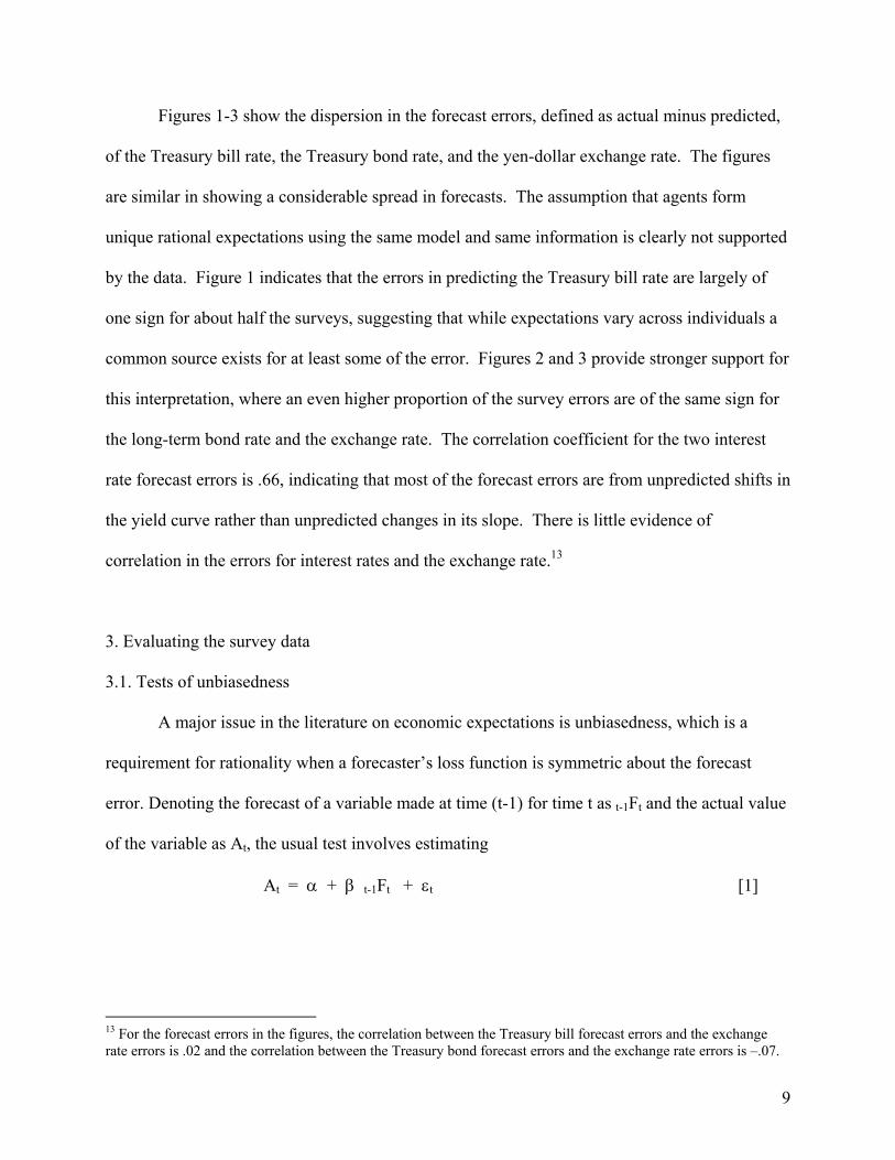
Figures 1-3 show the dispersion in the forecast errors, defined as actual minus predicted,

of the Treasury bill rate, the Treasury bond rate, and the yen-dollar exchange rate. The figures

are similar in showing a considerable spread in forecasts. The assumption that agents form

unique rational expectations using the same model and same information is clearly not supported

by the data. Figure 1 indicates that the errors in predicting the Treasury bill rate are largely of

one sign for about half the surveys, suggesting that while expectations vary across individuals a

common source exists for at least some of the error. Figures 2 and 3 provide stronger support for

this interpretation, where an even higher proportion of the survey errors are of the same sign for

the long-term bond rate and the exchange rate. The correlation coefficient for the two interest

rate forecast errors is .66, indicating that most of the forecast errors are from unpredicted shifts in

the yield curve rather than unpredicted changes in its slope. There is little evidence of

correlation in the errors for interest rates and the exchange rate.13

3. Evaluating the survey data

3.1. Tests of unbiasedness

A major issue in the literature on economic expectations is unbiasedness, which is a

requirement for rationality when a forecaster’s loss function is symmetric about the forecast

error. Denoting the forecast of a variable made at time (t-1) for time t as t-1Ft and the actual value

of the variable as At, the usual test involves estimating

At = α + β t-1Ft + εt [1]

13 For the forecast errors in the figures, the correlation between the Treasury bill forecast errors and the exchange rate errors is .02 and the correlation between the Treasury bond forecast errors and the exchange rate errors is –.07.

10

where εt is a random error term. A forecast series is unbiased if the joint hypothesis that α=0 and

β=1 cannot be rejected.14

As is well-known estimating [1] may produce misleading inferences when A and F are

nonstationary and not cointegrated since the error term will also be nonstationary, resulting in the

spurious regression problem noted by Granger and Newbold (1974). If the actual series is

nonstationary, an unbiased forecast must also be nonstationary and the two series must be

cointegrated with a cointegrating vector of zero and one. Liu and Maddala (1992) suggest a

restricted cointegration test when A and F are I(1): impose the restrictions α=0 and β=1 and use

the data to compute forecast errors; if the forecast errors are stationary, the restrictions are

supported and the forecasts are unbiased since the cointegrating vector is unique with only two

series.15 We perform the Liu-Maddala test below after first establishing whether A and F are

I(1).

To establish that the As – the daily Treasury bill, Treasury bond and exchange rate data

sampled at six-month intervals, the data frequency that matches our forecast series -- are I(1), we

perform unit root tests. Using levels data we cannot reject the hypothesis of a unit root for any of

the three series, but using first-differenced data we can reject the unit root hypothesis for all

three. Thus all three actual series appear to be I(1).16

To establish that the Fs -- the Treasury bill, Treasury bond and yen-dollar exchange rate

forecast series of the thirty-three economists listed in Table 2 who responded to at least 20

surveys -- are I(1), we perform 99 unit root tests (three forecast series for each of the thirty-three 14 Rationality tests often include a test that εt is not autocorrelated and may also include other information available at time (t-1) on the right hand side of equation [1]. Rationality requires that all such variables have zero coefficients. 15 Papers employing this restricted cointegration test include Hakkio and Rush (1989) and Osterberg (2000). 16 The ADF statistics using 1 lag for the levels of the Treasury Bill rate, Treasury bond rate, and yen-dollar exchange rate are -.867, -.970, and -2.396 respectively, indicating that each series has at least one unit root. The ADF statistics for the first differences are -4.950, -6.143, and -3.612 indicating that all series are I(1). Rose (1988) and Rapach and Weber (2004) also find that the nominal interest rate has a unit root while Baillie and Bollerslev (1989) report similar findings for nominal exchange rates.

11

economists). The t statistics for augmented Dickey-Fuller (ADF) unit root tests performed on

levels and first differences for individual forecasters are reported in the second column of Tables

3-5. Starred values indicate rejection of the unit root hypothesis at the 0.01, 0.05 or 0.10 levels

of significance. Of the 99 forecast series, 71 appear to be I(1) using the 10% significance level

or better.

To complete the Liu-Maddala test we impose the restriction that α=0 and β=1 on [1], use

the As and Fs to compute the forecast errors, and perform ADF tests to determine whether the

forecast errors are I(0). The third columns in Tables 3-5 report ADF t statistics for the case of a

zero intercept since the null hypothesis is that the residuals have an expected value of zero. Box-

Ljung Q statistics to test for serial correlation in the residuals appear beneath the t statistics. Of

the 99 forecast error series all but four are I(0) at the 10% level or better and only four show

evidence of serially correlated errors.

To pass the Liu-Maddala test the Fs must be I(1) and the forecast residuals must be I(0).

Nearly 60 % of the Treasury bill rate forecasts reported in Table 3 meet both criteria.17 In

addition, over three-quarters of the Treasury bond rate forecast series in Table 4 and two-thirds

of the exchange rate forecast series in Table 5 meet both criteria.18 Altogether, two-thirds (67) of

the 99 forecast series pass the Liu-Maddala test of unbiasedness. Moreover, the three series of

mean survey responses pass the Liu-Maddala test, as indicated in the last row of each table.

While the results of the Liu-Maddala tests are encouraging to proponents of forecaster

rationality, Lopes (2000) provides evidence that the power of their restricted cointegration test

17 About one-third of the forecast series appear to be I(0) despite the Treasury bill rate series being I(1). First differences of four other forecast series appear to be nonstationary even though the first difference of the Treasury bill rate series is stationary; the forecast errors in these four cases do appear stationary, however. For some individuals there are gaps, usually just one, in the forecast series. While Shin and Sarker (1993) find that occasional missing values do not change the asymptotic distribution of the standard Dickey-Fuller tests, our samples are small so that the results with a gap remain suspect. 18 Of the eleven exchange rate forecast series that failed, three had ten or fewer observations.

12

may be low, as is usual with unit root tests. He uses Monte Carlo techniques to show that a more

powerful test of unbiasedness in finite samples is a simple t-test for the hypothesis that a forecast

series’ mean forecast error is zero. Accordingly, we also report the mean forecast error and its t-

statistic in column 4 of each table. We fail to reject at the 10% level the null hypothesis of

unbiasedness for 73% of the Treasury bill forecast series, 67% of the Treasury bond forecast

series, and 88% of the exchange rate forecast series.19 Of the forecast series with test statistics

that reject the null, all of the Treasury bill rate and exchange rate forecast series and about two-

thirds of the Treasury bond rate forecast series err on the high side. Biased forecasts by some

forecasters did not serve to impart bias to the survey mean forecasts, however: the average

forecast errors of the survey mean forecasts were statistically indistinguishable from zero,

implying unbiasedness.

In summary, about two-thirds of the forecast series appear to be statistically unbiased, as

do all three series of mean survey responses. Economists whose forecasts appeared to be biased

usually overestimated the 6-month-ahead level of the Treasury bill, Treasury bond or yen-dollar

exchange rate, with overestimation occurring more frequently in predicting interest rates than

exchange rates. Based on the t-tests for unbiasedness at the 10% level, about 60 % of the survey

economists were statistically unbiased in their predictions of the Treasury bill, Treasury bonds

and exchange rate; about 10% made biased forecasts of one of the three rates; and the remaining

30% made biased forecasts of two series. No economist made biased predictions of all three

rates.20

19 At the less stringent 5% level, 80%, 73% and 91%, respectively, of the Treasury bill, Treasury bond, and exchange rate series fail to reject the null of unbiasedness. 20 If the less stringent 5% level is used to judge unbiasedness, 67% of the survey forecasters were statistically unbiased in their predictions of all three rates; about 6% made biased forecasts of one of the rates; and the remaining 27% made biased forecasts of two rates.

13

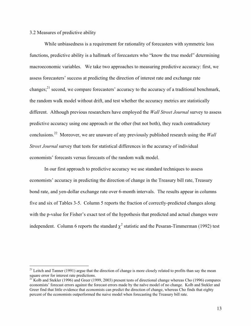
3.2 Measures of predictive ability

While unbiasedness is a requirement for rationality of forecasters with symmetric loss

functions, predictive ability is a hallmark of forecasters who “know the true model” determining

macroeconomic variables. We take two approaches to measuring predictive accuracy: first, we

assess forecasters’ success at predicting the direction of interest rate and exchange rate

changes;21 second, we compare forecasters’ accuracy to the accuracy of a traditional benchmark,

the random walk model without drift, and test whether the accuracy metrics are statistically

different. Although previous researchers have employed the Wall Street Journal survey to assess

predictive accuracy using one approach or the other (but not both), they reach contradictory

conclusions.22 Moreover, we are unaware of any previously published research using the Wall

Street Journal survey that tests for statistical differences in the accuracy of individual

economists’ forecasts versus forecasts of the random walk model.

In our first approach to predictive accuracy we use standard techniques to assess

economists’ accuracy in predicting the direction of change in the Treasury bill rate, Treasury

bond rate, and yen-dollar exchange rate over 6-month intervals. The results appear in columns

five and six of Tables 3-5. Column 5 reports the fraction of correctly-predicted changes along

with the p-value for Fisher’s exact test of the hypothesis that predicted and actual changes were

independent. Column 6 reports the standard χ2 statistic and the Pesaran-Timmerman (1992) test

21 Leitch and Tanner (1991) argue that the direction of change is more closely related to profits than say the mean square error for interest rate predictions. 22 Kolb and Stekler (1996) and Greer (1999, 2003) present tests of directional change whereas Cho (1996) compares economists’ forecast errors against the forecast errors made by the naïve model of no change. Kolb and Stekler and Greer find that little evidence that economists can predict the direction of change, whereas Cho finds that eighty percent of the economists outperformed the naive model when forecasting the Treasury bill rate.

14

statistic, also with a χ2 distribution with 1 degree of freedom, of the same independence

hypothesis.23

The directional accuracy tests suggest that the surveyed economists provide no useful

information.24 In forecasting the Treasury bill rate about two-thirds of economists predicted the

direction of change correctly more than half the time, but for no economist was the percentage of

correctly predicted directions significantly greater than expected by chance; moreover for a few,

the percentage was significantly lower. In predicting the Treasury bond rate, only about one-

third of economists forecasted directional change correctly more than half the time; nevertheless,

few predicted directional change less accurately than chance. The surveyed economists were

more successful in predicting directional change in the yen-dollar exchange rate: about 80

predicted correctly more than half the time; nevertheless none predicted correctly more often

than would be expected by chance. Finally, the survey means successfully predicted the

direction of Treasury bill rate and exchange-rate changes about as accurately as chance, but

predicted the direction of Treasury bond rate changes significantly more poorly than chance.

Thus, when set the task of predicting the direction of interest rate and exchange rate changes, the

surveyed economists acquit themselves modestly, at best.

In our second approach to predictive accuracy, we compare the accuracy of the surveyed

economists’ predictions to the accuracy of a model predicting that interest rates and exchange

rates follow a random walk without drift. Specifically, we computed the ratio of the mean square

errors (MSEs) of each economist’s forecast series to the MSEs of forecast series covering the 23 For each forecaster we constructed a contingency table with the number of times the forecaster predicted a decline and there was a decline, the number of times the forecaster predicted an increase and there was an increase, the number of times the forecaster incorrectly predicted a decrease, and the number of times the forecaster incorrectly predicted an increase. 24 We also performed the test of Cumby and Modest (1987), suggested by Stekler and Petrei (2003), in which the actual change is regressed on a binary variable taking the value of one if the forecaster predicted an increase and zero otherwise. These tests, not reported, also indicated that the respondents were unable to provide useful information on the direction of change.

15

same dates but using as forecasts the six-month-earlier actual values (that is, actuals on the last

business day in December and June, respectively, to forecast values for the last business day in

June and December, respectively; these actuals are usually published along side the forecasts in

the Wall Street Journal). The question becomes whether individual economists can outperform

the random walk model by achieving a ratio less than one. In addition to analyzing this ratio we

follow the recommendation of Fildes and Stekler (2002) and test for statistically significant

differences between individuals’ forecasts and random walk forecasts of no change using the

modified Diebold-Mariano (1995) test statistic proposed by Harvey et al. (1997). Specifically,

this statistic tests whether the mean difference between the squared forecast errors of the

economist and of the random walk model is significantly different from zero; this statistic has a

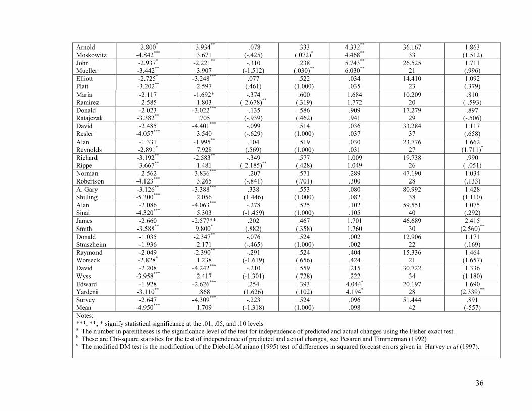
t-distribution under the null hypothesis that the mean is zero. We report our results in Tables 3-

5. The next-to-the last column reports the number of forecasts made by each economist together

with the sum of the squared forecast errors. The last column reports the ratio of each economist’s

MSE to the MSE from a random walk model and the Diebold-Marino statistic in parentheses.

The statistical evidence indicates that economists generally fail to beat and tend to be

statistically less accurate than the random walk model. Although in predicting the Treasury bill

rate eight of thirty-three economists achieve a MSE ratio less than one, the Diebold-Marino

statistics indicate that no economist forecasts significantly better than the random walk model

(i.e. a t-statistic that is significantly less than zero) and five do significantly worse at the 10%

level. In predicting the Treasury bond rate, no economist achieved a MSE ratio less than one;

moreover, about two-thirds of economists predicted significantly worse than a random walk

model, judging by the Diebold-Marino statistics (i.e., a t-statistic significantly greater than zero).

Accuracy in predicting the yen-dollar exchange was little better: no economist achieved a MSE

ratio less than one, and half predicted significantly worse than a random walk model, judged by

16

the Diebold-Marino statistics. Economists’ poor predictive ability is reflected in the survey

mean predictions. Although survey mean predictions of the Treasury bill rate achieve a MSE

ratio less than one, the survey mean predictions do not differ statistically from the random walk

predictions. Survey mean predictions of neither the Treasury bond rate nor the yen-dollar

exchange rate achieved MSE ratios less than one, and although the mean predictions of the

Treasury bond rate did not differ statistically from the random walk predictions, the mean

exchange-rate predictions were significantly worse than the random walk predictions.

Taken all together, the evidence on predictive ability suggests that agents who use

forecasts and prize accuracy would have suffered less disappointment by assuming that interest

rates and exchange rates stay at their last observed levels rather than by relying on forecasts from

the Wall Street Journal survey. The dismal predictive accuracy of many of the economists leads

us to ask whether the forecasts are systematically heterogeneous, possibly because some

economists face incentives to forecast large interest rate and exchange rate changes.

3.3. Tests of systematic heterogeneity of forecasts

Professional economists who are rational, who know the “true model,” and who, in

addition, have access to the same macroeconomic information relevant to forecasting interest

rates and exchange rates – as a priori reasoning suggests is probably the case – should produce

homogenous (identical) forecasts. In this section we examine whether forecasts of the

economists in the Wall Street Journal survey are homogeneous or systematically heterogeneous.

To test for homogeneity in forecasts we follow Ito (1990), who posits a fixed-effects

model. Ito models the forecast for time t of the jth economist, fj,t, as being a function of common

information, It, an individual effect represented by an individual-specific dummy variable, gj, and

a random error term, uj,t:

17

fj,t = f(It) + gj + uj,t . [2]

Ito assumes further that f(It) contains a constant so that the average of the gjs may be set to zero.

Averaging equation [2] across all economists and then subtracting the average from [2] yields:

fj,t – fAVE,t = gj + (uj,t - uAVE,t ) . [3]

Homogeneity of forecasts can be tested by estimating [3] on forecast data for individual

economists and testing that the estimated values of gj are identical across economists.25 26

Table 6 presents the results from estimating [3] using the Treasury bill rate, Treasury

bond rate and the yen-dollar exchange rate forecasts of the economists in the Wall Street Journal

survey and testing for forecast homogeneity. Like Ito (1990) we estimate [3] twice, first letting

the gjs represent dummy variables for individual economists and again letting the gjs represent

dummy variables for the economists’ sector of employment. Panels A and B, respectively,

report results from the two estimations. We report results for two sub-samples of economists,

one including all economists having at least six survey responses (Panel 1) and another including

all economists having at least twenty responses (Panel 2), the same economists whose forecasts

were examined in sections 3.1 and 3.2.27

The evidence in Table 6 overwhelmingly rejects the hypothesis of homogeneous

forecasts. In Panel A, F tests reject the null hypothesis of identical gj estimates for all economists

at the 0.01 level for all the data sets, indicating the presence of significant individual effects. In 25 An essentially identical approach is to regress the individual forecasts on a set of time dummies as well as a set of individual dummies and test for individual effects. 26 Ito uses [3] to test for heterogeneity in exchange rate forecasts made by Japanese economists. He finds that the data reject the hypothesis of homogeneous forecasts both when the gjs are individual dummy variables and when the gjs represent the industry of the economist’s employment. Ito also finds that economists employed in export industries have a depreciation bias whereas those employed in the import business have an appreciation bias, a pattern he terms the “wishful thinking” effect. MacDonald and Marsh (1996) also find evidence of heterogeneity across exchange rate forecasters from a large survey of European economists. In addition they report that the dispersion of forecasts is positively related to the volume of foreign exchange trading. MacDonald and Marsh report that the European economists are generally less accurate than a random walk for 3-month predictions but that a substantial number of economists beat a random walk when making 12-month forecasts. 27 These are unbalanced panels since participants change over time.

18

Panel B, coefficient estimates of five employment sectors appear (top number, standard errors

beneath) along with F tests of the null hypothesis that the estimated coefficients are identical

(reported in the last row). The data soundly reject the null for all data sets. The coefficient

estimates indicate that, compared with other economists, independent forecasters made

significantly lower forecasts of the Treasury bill and Treasury bond rate and significantly higher

forecasts of the yen-dollar exchange rate. Economists employed by securities firms also made

comparatively low forecasts of the Treasury bond rate, but not as low as economists employed

by independent firms. Economists affiliated with banks produced forecasts statistically

indistinguishable from the consensus, as did economists employed by econometric modeling

firms, except for yen-dollar exchange rate forecasts made by Panel 2, which were statistically

lower.

In summary, the evidence from the Wall Street Journal survey suggests that the

economists’ forecasts are indeed systematically heterogeneous. This finding leads us to

investigate whether individual forecasters behave strategically in making their forecasts.

3.4. Tests of strategic forecasting

Laster et al. (1999) and Lamont (2002) suggest that the incentive structure facing

professional economists potentially motivates them to supply heterogeneous forecasts.

Specifically, they argue that if economists are rewarded both for forecast accuracy and for

“standing out from the crowd,” economists may announce more extreme predictions than if they

were rewarded for forecast accuracy alone.28 To investigate this possibility we estimate a model

combining elements of Lamont (2002) and Laster et al. (1999):

28 Lamont (2002) models forecasters’ payoff function as follows: wj = R(|fj – a|, |fj – fc(-j)|)

19

|fj – fc(-j)|t = β0 + β1 AGEj,t + β2 AGEj,t* MODELj,t + β3 AVEDEV(-j)t

+ β4 OWNj,t + ∑ γi Di,t + εj,t [4]

Following Lamont our dependent variable – a measure of “standing out from the crowd” – is the

absolute value of the difference between an individual economist’s time t forecast and the

average time t forecast omitting that economist’s forecast. AGE is the number of years an

economist had participated in the Wall Street Journal survey at the time of survey t while the

interaction term AGE*MODEL allows the effect of an economist’s age to differ if the economist

is employed by an econometric modeling firm. 29 AGE is included to control for changing

incentive structures: incentives might encourage young forecasters to make extreme forecasts so

as to gain publicity while encouraging older forecasters to make less extreme forecasts so as to

protect the reputations; alternatively, incentives might encourage young forecasters to make less

extreme forecasts so as to hide their inexperience while encouraging seasoned, secure forecasters

to make more radical forecasts. AVEDEV(-j) is the average absolute deviation of the forecasts

from the mean, omitting the jth economist; this latter variable controls for variations in the spread

of the forecasts over time. The dummy variable, OWN, equals one if an economist is employed

at a firm that bears his name. Finally, following Laster et al., we add dummy variables for the

industry employing the jth economist at the time of survey t, the Djts. Our industries include

banks, securities firms, finance departments of corporations, econometric modelers, and

economists employed by independent firms not bearing the economists’ names, similar to Laster

where wj is the payoff to forecaster the jth forecaster, |fj – a| is the absolute value of the jth forecaster’s forecast from the actual value, and |fj – fc(-j)| is the absolute value of the jth forecaster’s forecast from the consensus forecast, omitting the jth forecaster’s forecast. Lamont assumes the partial derivative of R with respect to the first argument, R1, is negative: inaccurate forecasts reduce a forecaster’s payoff. But he allows that the partial derivative of R with respect to the second argument, R2, is an empirical question. 29 Lamont found that this variable was important and that the effect of age was not significant for forecasts from econometric models.

20

et al. The hypothesis that economists behave strategically is supported by statistically significant

coefficients on AGE, AGE*MODEL, OWN, and the Djts, as well as by statistical differences

among the estimated coefficients of the Djts.

Table 7 presents estimates of [4] using the Treasury bill rate, Treasury bond rate and the

yen-dollar exchange rate forecasts of the economists in the Wall Street Journal survey. As in the

previous section we report estimates for two sub-samples of economists, one including all

economists having at least six survey responses (Panel 1) and another including all economists

having at least twenty responses (Panel 2), the same economists whose forecasts were examined

in sections 3.1 and 3.2.

The Table 7 estimates show overwhelming evidence of strategic behavior by economists

in the form of statistically significant estimated coefficients of AGE, OWN and several of the

Djts, as well as statistical differences among the Djts. The estimated coefficients of AGE are

negative and usually statistically significant, implying that economists make less extreme

forecasts the longer they are surveyed.30 This age effect holds for all economists including those

employed by econometric modeling firms, since the estimated coefficient of AGE*MODEL

never achieves significance. Though pervasive, the estimated age effects are small in absolute

terms: compared with a first-time respondent, an economist in the survey for 10 years (20

surveys) is about 4 basis points closer to the mean interest rate forecast and a little less than one

yen closer to the mean exchange rate forecast. Larger in absolute terms is the effect of

employment by a forecasting firm bearing one’s name: forecasts of such economists deviate

more from the mean forecasts than forecasts of other economists by amounts ranging from 13 to

30 As noted above, the Wall Street Journal does not systematically drop forecasters with poor records so a negative coefficient should not be due to a survivorship bias. It is possible, however, that people who make extreme and inaccurate forecasts drop out to avoid negative publicity. We also estimated a model with age and AVEDEV(-j) as explanatory variables for each of the individuals listed in Table 2. Age was statistically significant at the .10 level for only about one-third of the panel and was negative in most cases. No individual had significantly positive coefficients on age for all three variables being forecasted.

21

22 basis points for the interest rates and 1.7 yen, on average, for the exchange rate. The name

effect appears to drive economists’ strategic behavior rather than independence per se: only in

forecasting the Treasury bond rate did economists employed by independent firms named for

others make forecasts statistically more extreme than the consensus, and even then the effect was

absolutely small. Surveyed economists employed by banks appeared to make less extreme

forecasts than other economists, judging from the consistently negative and statistically

significant estimated coefficients of Banks. Economists employed by securities firms,

corporations and econometric modeling firms also tended to make less extreme forecasts,

judging from the generally negative although inconsistently significant estimated coefficients of

their respective dummy variables. When the hypothesis that economists’ forecasts deviated

equally from the consensus regardless of employment is tested, F statistics soundly and

universally reject the hypothesis. Because it seems unlikely that economists in different

industries had differential access to the macroeconomic data needed to make interest rate and

exchange rate forecasts, we conclude that incentive structures encourage economists employed in

different industries to supply heterogeneous forecasts, with economists from firms bearing their

own names being more likely to make extreme forecasts because they gain the most from being

right when others are wrong.31

3.5 Discussion of results

We believe that the results presented in sections 3.1 – 3.4 present a consistent story. Our

findings from section 3.1 – that 30% of economists produced biased forecasts, generally in the

upward direction – and from section 3.2 – that economists generally failed to forecast as

31 We also estimated equation [4] allowing for individual fixed effects or individual random effects. These models gave similar estimates for the effects of AGE and AVEDEV but wiped out the statistical significance of the industry effects. Since individuals change industries occasionally in our sample, as indicated in Table 2, the industry differences appear to be captured by the individual effects.

22

accurately as the random walk model and sometime forecasted less accurately – is consistent

with the heterogeneity of forecasts we found in section 3.3. When we tested for evidence of

strategic behavior by economists in section 3.4 by using a synthesis of the Lamont (2002) and

Laster et al. (1999), we obtained some results similar to theirs. Like Lamont and Laster et al. we

found that economists from independent firms tend to make more extreme forecasts and, like

Lamont, we found that economists whose firms bear their names make forecasts that consistently

deviate more from the survey mean than other economists. But whereas Lamont found evidence

that economists make more extreme forecasts the longer they are surveyed, we found the

opposite to be true: the estimated coefficients of AGE are consistently negative and usually

statistically significant.

Although our results on strategic behavior bear some similarities to Lamont and Laster et

al.’s, we believe it is important to note the advantages of the Wall Street Journal survey data on

interest rates and exchange rates for testing strategic behavior compared with Business Week

survey data used by Lamont and the Blue Chip Economic Indicators data used by Laster et al.

Although the Business Week survey publishes forecasts of economists by name, Lamont studied

economists’ forecasts of real GDP growth, inflation and unemployment, all of which are subject

to revision, which raises the issue of which values economists were forecasting. Laster et al.

also study economists’ forecasts of real GDP growth, so the caveats that apply to Lamont apply

to Laster et al. as well. In addition, the Blue Chip Indicators data Laster et al. use groups

forecasters by industry rather than identifying them individually; hence the incentives to forecast

strategically are not as strong.

Our finding that the Wall Street Journal’s panel of economists cannot predict changes in

interest rates and exchange rates more accurately than a random walk model is not surprising,

23

given the efficiency of financial markets. What is perhaps surprising is that so many of the panel

forecast significantly worse than the random walk model. The explanation of these results we

favor is that many of the economists face incentives that reward the exceptionally right guess but

do not equally penalize the exceptionally wrong guess. An alternative explanation is that even if

the economists know the random walk model to be more accurate over time, this leaves them

with no story to spin about their forecasts. Always telling customers that you predict no change

in interest rates or exchange rates may simply be too truthful to keep one employed.

4. Conclusions

While widespread public interest in forecasts of macroeconomic variables has led

professional economists to put considerable effort in generating forecasts, less effort has gone

into assessing the quality of these forecasts. The theory of rational expectations implies that

professional economists’ forecasts should be unbiased and identical given access to the same

information and similar incentives with respect to predictive accuracy. Previous studies

employing survey data of professional economists’ forecasts to assess forecast quality have

tended to lack comprehensiveness, suffer from data problems, or produce inconclusive results.

This paper has sought to help fill the void by using semi-annual survey data from the

Wall Street Journal’s panel of economists to study interest rate and exchange rate forecasts of

individual economists. We found that while about 60% of the surveyed economists produced

unbiased estimates, virtually all failed to make 6-month ahead forecasts of the Treasury bill rate,

Treasury bond rate and yen-dollar exchange rate that beat a naïve random walk model for

accuracy, and many made forecasts significantly less accurate than the random walk model.

When we tested for homogeneity of interest rate and exchange rate forecasts, we found them to

be systematic heterogeneous. In particular, we found that independent economic forecasters

(those not employed by banks, security firms, corporations’ finance departments, or econometric

24

model firms) made significantly lower forecasts of the Treasury bill rate and Treasury bond rate

and significantly higher forecasts of the yen-dollar exchange rate. Evidence of systematically

heterogeneous forecasts led us to consider whether economists faced economic incentives to

produce heterogeneous forecasts. When we estimated an incentives model combining elements

of models estimated by Lamont (2002) and Laster et al. (1999), we found evidence that

economists who would be expected to gain the most from favorable publicity – those employed

by firms named for them – make more extreme forecasts, whereas economists employed by other

institutions tend to make more conservative, less extreme forecasts. We found no evidence that

economists become more radical with age. If anything, experienced economists appear to

preserve their reputations by deviating less from the consensus forecast than inexperienced

economists.

25

References

Aggarwal, R., S. Mohanty and F. Song, “Are Survey Forecasts of Macroeconomic Variables Rational?” Journal of Business, 68(1) , January 1995, 99-119. Anderson, T., T. Bollerslev, F.X. Diebold, and C. Vega, “Micro Effects of Macro Announcements: Real-Time Price Discovery in Foreign Exchange,” American Economic Review, 93(1), March 2003, 38-62. Baillie, R.T. and T. Bollerslev, “Common Stochastic Trends in a System of Exchange Rates,” Journal of Finance, 44(1), March 1989, 167-181. Batchelor, R. and P. Dua, “Blue Chip Rationality Tests,” Journal of Money, Credit, and Banking, 23(4), November 1991, 692-705. Bonham, C.S., and R.H. Cohen, “To Aggregate, Pool, or Neither: Testing the Rational- Expectations Hypothesis Using Survey Data,” Journal of Business and Economic Statistics, 19(3), July 2001, 278-291. Carroll, C.D. “Macroeconomic Expectations of Households and Professional Forecasters.” Quarterly Journal of Economics, 118(1), February 2003, 269-298. Cho, D.W. “Forecast Accuracy: Are Some Business Economists Consistently Better Than Others?” Business Economics; 31(4), October 1996, 45-49. Croushore, D. “Evaluating Inflation Forecasts,” Working Paper No. 98-14, Federal Reserve Bank of Philadelphia, June 1998. Cumby, R.E. and D.M. Modest, “Testing for Market Timing Ability: A Framework for Forecast Evaluation,” Journal of Financial Economics, 19(1), September 1987, 169-189. Diebold, F.X. and R.S. Mariano, “Comparing Predictive Accuracy,” Journal of Business and Economic Statistics, 13(3), July 1995, 253-263. Eisenbeis, R., D. Waggoner, and T. Zha, “Evaluating Wall Street Journal Survey Forecasters: A Multivariate Approach,” Business Economics, 37(3), July 2002, 11-21. Ehrbeck, T. and R. Waldmann. “Why are Professional Forecasters Biased? Agency Versus Behavioral Explanations.” Quarterly Journal of Economics, 111(1), February 1996, 21-40. Figlewski, S. and P. Wachtel, “The Formation of Inflationary Expectations,” Review of Economics and Statistics, 63(1), February 1981, 1-10. Frankel, J.A. and K.A. Froot, “Using Survey Data to Test Standard Propositions Regarding Exchange Rate Expectations,” American Economic Review, 77(1), March 1987, 133-153.

26

Granger, C.W.J. and P. Newbold, “Spurious Regressions in Econometrics,” Journal of Econometrics, 2(2), July 1974, 111-120. Greer, M. R. “Assessing the Soothsayers: An Examination of the Track Record of Macroeconomic Forecasting,” Journal of Economic Issues, 33(1), March 1999, 77-94. Greer, M.R. “Directional Accuracy Tests of Long-Term Interest Rate Forecasts,” International Journal of Forecasting, 19(2), April-June 2003, 291-298. Hakkio, C.S. and M. Rush, “Market Efficiency and Cointegration: An Application to the Sterling and Deutschmark Exchange Markets,” Journal of International Money and Finance, 1989, 8, 75-88. Harvey D., S. Leybourne, and P. Newbold, “Testing the Equality of Prediction Mean Squared Errors,” International Journal of Forecasting, 13(2), June 1997, 281-291. Ito, T. “Foreign Exchange Rate Expectations: Micro Survey Data,” American Economic Review, 80(3), June 1990, 434-449. Keane, M.P. and D.E. Runkle, “Testing the Rationality of Price Forecasts: New Evidence from Panel Data,” American Economic Review, 80(4), September 1990, 714-735. Kolb, R.A. and H.O. Stekler, “How Well Do Analysts Forecast Interest Rates?” Journal of Forecasting, 15(5), September1996, 385-394. Lamont, O., “Macroeconomic Forecasts and Microeconomic Forecasters,” Journal of Economic Behavior and Organization,48(3), July 2002, 265-280.

Laster, D., P. Bennett, and I.S. Geoum. “Rational Bias in Macroeconomic Forecasts.” Quarterly Journal of Economics, 114(1), February 1999, 293-318.

Leitch, G. and J.E. Tanner, “Economic Forecast Evaluation: Profits Versus the Conventional Error Measures,“ American Economic Review, 84(3), June 1991, 580-590.

Liu, P.C. and G.S. Maddala, “Rationality of Survey Data and Tests for Market Efficiency in the Foreign Exchange Market,” Journal of International Money and Finance, 11(4), August 1992, 366-381. Lopes, A. C. B.D., “On the ‘Restricted Cointegration Test’ as a Test of the Rational Expectations Hypothesis,” Applied Economics, 30(2), February 1998, 269-278. MacDonald, R. “Expectation Formation and Risk in Three Financial Markets: Surveying What the Surveys Say,” Journal of Economic Surveys, 14(1), February 2000, 69-100. MacDonald, R. and I.W. Marsh, “Currency Forecasters are Heterogeneous: Confirmation and Consequences,” Journal of International Money and Finance, 15(5) October 1996, 665-685.

27

Osterberg, W.P. “New Results on the Rationality of Survey Measures of Exchange-Rate Expectations,” Economic Review, Federal Reserve Bank of Cleveland, 36(1), Quarter 1, 2000, 14-21. Pesaran, M.H. and A. Timmerman, “A Simple Nonparametric Test of Predictive Performance,” Journal of Business and Economic Statistics, 10(4), October 1992, 461-465. Pons-Novell, J. “Strategic Bias, Herding Behaviour and Economic Forecasts,” Journal of Forecasting, 22(1), January 2003, 67-77. Rapach, D.E. and C.E. Weber, “Are Real Interest Rates Really Nonstationary?” Journal of Macroeconomics, 26(3), September 2004, 409-430 Rose, A.K. “Is the Real Interest Rate Stable?” Journal of Finance, 43(8), December 1988, 1095-1112. Scharfstein, D.S. and J.C. Stein. “Herd Behavior and Investment,” American Economic Review, 80(3), June 1990, 465-479. Schirm, D.C. “A Comparative Analysis of the Rationality of Consensus Forecasts of U.S. Economic Indicators,” Journal of Business, 76(4), October 2003, 547-561. Shin, D.W. and S. Sarker, “Testing for a Unit Root in an AR(1) Time Series Using Irregularly Observed Data,” Working paper, Oklahoma State University, 1993. Stekler, H.O. and G. Petrei, “Diagnostics for Evaluating the Value and Rationality of Economic Forecasts,” International Journal of Forecasting, 19(4), October-December 2003, 735-742. Thomas, L.B., “Survey Measures of Expected U.S. Inflation,” Journal of Economic Perspectives, 13(4), Autumn 1999, 125-44.

28

Figure 1

Forecast Errors of the Treasury Bill Rate

-6

-5

-4

-3

-2

-1

0

1

2

3

4

5

0 10 20 30 40

Survey Number

Fore

cast

Err

or, i

n Pe

rcen

tage

Poi

nts

Note: Forecast errors are measured as the actual rate minus forecasters’ predictions on the survey date, six months earlier. Forecast

errors are shown for the 42 surveys beginning with January 1982 and ending with July 2002.

29

Figure 2

Forecast Errors for theTreasury Bond Rate

-5

-4

-3

-2

-1

0

1

2

3

4

5

0 10 20 30 40

Survey Number

Fore

cast

Err

or, i

n Pe

rcen

tage

Poi

nts

See notes to Figure 1.

30

Figure 3

Forecast Errors for the Yen-Dollar Exchange Rate

-80

-60

-40

-20

0

20

40

10 15 20 25 30 35 40 45

Survey Number

Fore

cast

Err

or, Y

en p

er d

olla

r

Note: Forecasts of the yen-dollar exchange rate were added to the Wall Street Journal survey in January 1989. Forecast errors are shown for the 28 surveys from January 1989 to July 2002, which correspond to survey numbers 15-24 in our sample.

31

Table 1 Summary Statistics for Survey Forecasts

Survey Date

Treasury bill Rate

Treasury bond Rate

Yen-Dollar Rate

year_mo Mean S.D.

Range N

Actual Mean S.D.

Range N

Actual Mean S.D.

Range N

Actual

1982_01

11.06 2.05

8.8-16 12

12.76

13.05 1.13

11.5-16 12

13.91

1982_07

11.61 .54

10.5-12.5 14

7.92

13.27 .35

12.5-13.75 14

10.43

1983_01

7.37 .94

5.5-9.625 17

8.79

10.11 .71

9-11.625 17

11.01

1983_07

8.60 .89

6-10 17

8.97

10.59 .60

9-11.75 17

11.87

1984_01

8.72 .64

7-10 24 9.92

11.39 .68

9.5-12.5 13.64

1984_07

10.62 .76

8.5-12 24 7.85

13.75 .85

11-14.75 24 11.54

1985_01

8.56 .98

6.5-10.6 24 6.83

11.60 .80

10-13.25 24 10.47

1985_07

7.31 .82

5.5-8.75 25 7.05

10.51 .83

8.5-11.8 25 9.27

1986_01

6.96 .58

5.5-7.75 25 5.96

9.45 .63

8-10.5 25 7.24

1986_07

6.02 .51

5-7 30 5.67

7.41 .51

6.5-8.25 30 7.49

1987_01

4.98 .48

4.1- 6 35 5.73

7.05 .53

5.88-8 35 8.51

1987_07

5.91 .50

4.25-6.63 35 5.68

8.45 .66

5.88-9.4 35 8.95

1988_01

5.70 .58

4-6.6 36 6.56

8.65 .71

6.8-9.75 36 8.87

1988_07

6.78 .39

5.8-7.6 32 8.1

9.36 .56

8-10.25 32 9

1989_01

8.29 .60

7.25-9.5 38 7.99

9.25 .49

8.25-10.5 38 8.05

121.37 6.15

110-135 38 144

1989_07

7.76 .52

6.4-9.1 38 7.8

8.12 .48

7.4-10 38 7.98

136.53 8.47

120-135 38 143.8

1990_01

7.03 .48

5.5-8 40 8

7.62 .35

7-8.4 40 8.41

137.78 6.81

120-155 40 152.35

1990_07

7.56 .43

6-8.5 40 6.63

8.16 .40

7.25-9 40 8.26

149.78 7.14

140-170 40 135.75

1991_01

6.14 .42

4.9-7.03 40 5.71

7.65 .46

6-8.5 40 8.42

133.65 9.69

120-170 40 137.9

1991_07

5.84 .35

5-6.6 40 3.96

8.22 .38

7.3-9 40 7.41

140.78 5.61

130-155 40 124.9

1992_01

3.80 .34

2.75-4.5 42 3.65

7.30 .37

6-8 42 7.79

127.64 8.07

115-160 42 125.87

1992_07

3.54 .39

2.9-4.3 42 3.15

7.61 .38

6.45-8.3 42 7.4

127.33 7.07

115-147 42 124.85

1993_01

3.41 .32

2.7-4.45 44 3.1

7.44 .33

6.7-8.4 44 6.68

127.70 7.07

115-157 44 106.8

32

Table 1, continued

Survey Date

Treasury bill Rate

Treasury bond Rate

Yen-Dollar Rate

year_mo Mean S.D.

Range N

Actual Mean S.D.

Range N

Actual Mean S.D.

Range N

Actual

1993_07

3.34 .31

2.37-4 44 3.07

6.84 .35

5.99-7.5 44 6.35

112.16 6.44

100-130 44 111.7

1994_01

3.40 .28

2.5-4 51 4.26

6.26 .38

5.5-7 51 7.63

113.10 5.90

100-140 49 98.51

1994_07

4.67 .60

3.15-8 58 5.68

7.30 .39

6.5-8.1 58 7.89

106.85 3.69

99-115 52 99.6

1995_01

6.50 .49

4.89-7.5 59 5.6

7.94 .38

6.8-8.6 59 6.63

104.09 4.00

95-117 57 84.78

1995_07

5.44 .56

4-7.04 62 5.1

6.61 .52

5.75-8.05 62 5.96

89.23 4.24

80-100 60 103.28

1996_01

4.98 .45

3.5-6.25 64 5.18

6.03 .44

5-7.5 64 6.9

104.71 4.56

87-112 62 109.48

1996_07

5.31 .40

4.18-6.3 58 5.21

6.86 .47

5.45-7.7 58 6.65

109.99 4.25

98-120 56 115.77

1997_01

5.16 .41

4.4-6.5 57 5.25

6.52 .52

5-7.6 57 6.8

113.45 4.15

100-122 55 114.61

1997_07

5.41 .35

4.58-6.3 55 5.36

6.79 .40

5.8-7.5 55 5.93

114.89 4.66

105-125 54 130.45

1998_01

5.18 .30

4.25-6 56 5.1

6.02 .37

5.2-6.95 56 5.62

130.41 7.03

115-145 54 138.29

1998_07

5.08 .25

4.25-5.5 55 4.48

5.72 .36

5-6.38 55 5.09

141.28 10.38

120-172 53 113.08

1999_01

4.20 .33

3.5-5 54 4.78

5.05 .44

4.25-6.8 54 5.98

122.77 9.93

100-150 52 120.94

1999_07

4.89 .34

3.7-5.6 54 5.33

5.83 .48

4.5-7 54 6.48

124.75 7.19

110-145 53 102.16

2000_01

5.58 .35

4.5-6.25 53 5.88

6.38 .40

4.8-7.13 53 5.9

105.32 7.20

90-132 53 106.14

2000_07

6.11 .41

5-6.9 53 5.89

6.01 .39

5-7.1 53 5.46

105.34 5.94

90-126 53 114.35

2001_01

5.36 .38

4.3-6.4 52 3.65

5.35 .31

4.5-6 54 5.75

113.21 5.39

97-127 53 124.73

2001_07

3.39 .42

2.7-5.35 54 1.74

5.28 .40

4-6 54 5.07

126.48 6.18

113-140 54 131.04

2002_01

1.89 .32

1.25-2.5 55 1.7

5.06 .51

3.75-6 55 4.86

132.76 7.34

117-115 55 119.85

2002_07

2.19 .33

1.5-3 54 1.22

5.21 .36

4-6.25 55 3.83

123.58 6.53

110-143 55 118.75

Note: Survey respondents are asked early in January and July for their forecasts for the last business day of July and December, respectively. The mean, standard deviation (S.D.) and range of the forecasts in each survey are shown. The number of respondents (N) varies across surveys. The actual values of the variables forecasted are shown in the “Actual” column.

33

Table 2 Participants Responding To At Least Twenty Surveys

Person

Firm

start

end

gaps

missing dates

David Berson Fannie Mae 199001 200207 0 Paul Boltz T. Rowe Price 198401 199801 0 Philip Braverman 198401 199901 0 Briggs Schaedle 198401 198807 Irving Securities 198901 198907 DKB Securities 199001 199901 Dewey Daane Vanderbilt Univ. 198807 200207 0 Robert Dederick Northern Trust 198607 199607 0 Gail Fosler Conference Board 199101 200207 0 Maury Harris 198607 200207 0 Paine Webber Inc. 198607 200007 UBS Warburg 200107 200207 Richard Hoey 198401 199401 1 199107 A.G. Becker 198401 198407 Drexel Burnham 198501 199101 Dreyfus Corp. 199201 199401 Stuart G. Hoffman PNC Bank, Fin Serv 198801 200207 1 199401 William Hummer 199301 200207 0 Wayne Hummer 199301 199707 Hummer Invest. 199807 200207 Edward Hyman 198301 200207 1 198901 C.J. Lawrence 198301 199107 ISI Group 199201 200207 Saul Hymans Univ. of Michigan 198607 200207 0 for yen:199407 199607 199807 199901 David Jones Aubrey G. Lanston 198201 199301 0 Irwin Kellner ManuHan-Chem-Chase 198201 199701 1 198407 Carol Leisenring CoreStates Finl. 198707 199801 0 Alan Lerner 198201 199307 1 198401 Bankers Trust 198201 199207 Lerner Consulting 199301 199301 Mickey Levy 198507 200207 0 Fidelity Bank 198507 199107 CRT Govt. Securities 199201 199307 NationsBank Cap. Mk 199401 199807 Bank of America 199901 200207 Arnold Moskowitz 198401 200007 1 198807 Dean Witter 198401 199107 Moskowitz Capital 199201 200007 John Mueller LBMC 199107 200207 2 199401 199507 Elliott Platt Donaldson Lufkin(DLJ) 198807 200001 1 199207 Maria Ramirez 199207 200207 1 199401 Ramirez Inc. 199207 199307 MF Ramirez 199407 200107 MFR 200201 200207 Donald Ratajczak 198701 200101 0 Georgia State Univ. 198701 200001 Morgan Keegan 200007 200101 David Resler 198407 200207 0 First Chicago 198407 198701? Nomura Securities I 198707 200207 Alan Reynolds 198607 200001 1 199501 Polyconomics 198607 199107 Hudson Institute 199201 200001 Richard Rippe 199001 200207 0 Dean Witter 199001 199107 Prudential Securities 199201 200207

34

Table 2, continued Participants Responding To At Least Twenty Surveys

Person

Firm

start

end

gaps

missing dates

Norman Robertson 198201 199601 1 199407 Mellon Bank 198207 199207 Carnegie Mellon 199301 199601 A. Gary Shilling Shilling & Co. 198201 200207 4 198307 198401 198901 198907 Alan Sinai 198201 200207 198807 199707 Data resources 198207 198307 Lehman Bros Shearson 198401 198801 The Boston Co.(Lehman) 198901 199207 Economic Advisors Inc (Lehman) 199301 199307 Lehman Brothers 199401 199701 WEFA Group 199801 199801 (Primark) Decision Economic 199807 200207 James Smith 198701 200207 2 198807 199401 UT-Austin 198701 198801 Univ. of N.C. 198901 199901 Natl Assn of Realtors 199907 200001 Univ. of N.C. 200007 200207 Donald Straszheim 198607 200207 11 198807 199707-200201 Merril Lynch 198607 199701 Strszheim Global Advisors 200207 200207 Raymond Worseck A.G. Edwards 198901 199901 0 David Wyss 198401 200207 4 198807 199407(yen) 200001-200101 Data Resources 198401 199907 Standard & Poor's (McGraw-Hill) 200107 200207 Edward Yardeni 198607 200007 1 198807 Prudential Bache 198607 199107 C.J. Lawrence 199201 199507 Deutsche Bank 199601 200007

35

Table 3 Unbiasedness and Accuracy of Treasury Bill Rate Forecasts

Individual

Liu-Maddala Restricted CointegrationTest of Unbiasedness

ADF(forecast) ADF(error)

ADF(∆forecast) Q(4)

Mean Forecast Error and t-test for

Unbiasedness

Fraction of Correct

Directions (p-value for

independence test)a

χ2 and Pesaran-Timmerman

Tests of Independenceb

Accuracy Σ (A-F)2 MSE Ratio to Random Walk n (Modified DM

statistic)c

David Berson

-3.149**

-3.030** -2.426**

4.260 -.351

(-2.369)** .577

(.453) .735 .765

17.488 26

.877 (-.754)

Paul Boltz

-2.720*

-2.833* -2.901***

.541 -.460

(-2.257)** .517

(.694) .348 .361

39.928 29

1.929 (1.810)*

Phillip Braverman

-3.768***

-3.931*** -4.680***

1.696 .203

(1.027) .483

(.368) 1.178 1.217

37.695 31

1.780 (1.225)

Dewey Daane

-2.289 -3.632**

-2.775***

2.200 -.382

(-2.584)** .517

(.694) .348 .361

21.981 29

.984 (-.066)

Robert Dederick

-1.559 -2.984**

-2.758***

2.752 -.084

(-.477) .524

(1.000) ..029 .031

13.270 21

1.008 (.039)

Gail Fosler

-3.171**

-4.061*** -3.313***

6.633 -.514

(-2.776)** .542

(.653) .697 .728

25.241 24

1.402 (1.370)

Maury Harris

-1.571 -3.275**

-3.185***

2.009 -.092

(-.639) .545

(.728) .308 .318

22.264 33

.958 (-.211)

Richard Hoey

-1.660 -2.334

-2.290** 3.560

-.425 (-1.765)*

.350 (.613)

.848

.892 25.598

20 1.674

(1.698) Stuart G. Hoffman

-1.954 -3.870***

-3.245*** .842

-.164 (-1.043)

.621 (.264)

1.830 1.896

20.978 29

.966 (-.160)

William Hummer

-2.047 -2.516

-1.819*

2.019 -.380

(-2.190)** .600

(.582) 1.250 1.316

14.282 20

1.038 (.220)

Edward Hyman

-1.784 -4.026***

-4.399***

6.248 .289

(1.672) .564

(.706) ..416 .427

47.690 39

1.515 1.076

Saul Hymans

-2.545 -3.900***

-2.828*** 8.681

-.196 (-1.210)

.455 (.733)

.203

.209 28.911

33 1.245

(2.010)*

David Jones

-1.701 -4.117***

-2.770*** 4.205

-.316 (-.882)

.391 (.400)

1.245 1.301

67.325 23

1.533 (1.052)

Irwin Kellner

-3.635** -4.854***

-4.828*** 1.172

-.102 (-.421)

.333 (.141)

3.274*

3.387* 51.619

30 1.190

(1.480) Carol Leisenring

-1.669 -3.114**

-2.430**

3.773 .025

(.147) .455

(1.000) .188 .197

12.913 22

.982 (-.081)

Alan Lerner

-1.765 -5.333***

-3.887*** 6.775

-.583 (-1.990)*

.652 (.221)

1.806 1.888

51.187 23

1.188 (.505)

Mickey Levy

-2.409 -4.476***

-3.810*** 3.691

-.152 (-.991)

.514 (1.000)

.000

.000 28.724

35 1.175 (.888)

36

Arnold Moskowitz

-2.800*

-4.842*** -3.934** 3.671

-.078 (-.425)

.333 (.072)*

4.332** 4.468**

36.167 33

1.863 (1.512)

John Mueller

-2.937* -3.442**

-2.221** 3.907

-.310 (-1.512)

.238 (.030)**

5.743**

6.030** 26.525

21 1.711 (.996)

Elliott Platt

-2.725* -3.202**

-3.248*** 2.597

.077 (.461)

.522 (1.000)

.034

.035 14.410

23 1.092 (.379)

Maria Ramirez

-2.117 -2.585

-1.692* 1.803

-.374 (-2.678)**

.600 (.319)

1.684 1.772

10.209 20

.810 (-.593)

Donald Ratajczak

-2.023 -3.382**

-3.022*** .705

-.135 (-.939)

.586 (.462)

.909

.941 17.279

29 .897

(-.506) David Resler

-2.485 -4.057***

-4.401*** 3.540

-.099 (-.629)

.514 (1.000)

.036

.037 33.284

37 1.117 (.658)

Alan Reynolds

-1.331 -2.891*

-1.995** 7.928

.104 (.569)

.519 (1.000)

.030

.031 23.776

27 1.662

(1.711)*

Richard Rippe

-3.192** -3.667**

-2.583** 1.481

-.349 (-2.185)**

.577 (.428)

1.009 1.049

19.738 26

.990 (-.051)

Norman Robertson

-2.562 -4.123***

-3.836*** 3.265

-.207 (-.841)

.571 (.701)

.289

.300 47.190

28 1.034 (.133)

A. Gary Shilling

-3.126** -5.300***

-3.388*** 2.056

.338 (1.446)

.553 (1.000)

.080

.082 80.992

38 1.428

(1.110) Alan Sinai

-2.086 -4.320***

-4.063*** 5.303

-.278 (-1.459)

.525 (1.000)

.102

.105 59.551

40 1.075 (.292)

James Smith

-2.660 -3.588**

-2.577** 9.800*

.202 (.882)

.467 (.358)

1.701 1.760

46.689 30

2.415 (2.560)**

Donald Straszheim

-1.035 -1.936

-2.347** 2.171

-.076 (-.465)

.524 (1.000)

.002

.002 12.906

22 1.171 (.169)

Raymond Worseck

-2.049 -2.828*

-2.390** 1.238

-.291 (-1.619)

.524 (.656)

.404

.424 15.336

21 1.464

(1.657) David Wyss

-2.208 -3.958***

-4.242*** 2.417

-.210 (-1.301)

.559 (.728)

.215

.222 30.722

34 1.336

(1.180) Edward Yardeni

-1.928 -3.110**

-2.626*** .868

.254 (1.626)

.393 (.102)

4.044*

4.194* 20.197

28 1.690

(2.339)**

Survey Mean

-2.647 -4.950***

-4.309***

1.709 -.223

(-1.318) .524

(1.000) .096 .098

51.444 42

.891 (-557)

Notes: ***, **, * signify statistical significance at the .01, .05, and .10 levels a The number in parentheses is the significance level of the test for independence of predicted and actual changes using the Fisher exact test. b These are Chi-square statistics for the test of independence of predicted and actual changes, see Pesaren and Timmerman (1992) c The modified DM test is the modification of the Diebold-Mariano (1995) test of differences in squared forecast errors given in Harvey et al (1997).

37

Table 4 Unbiasedness and Accuracy of Treasury bond Rate Forecasts

Individual Liu-Maddala Restricted Cointegration Test of Unbiasedness

ADF(forecast) ADR(error) ADF(∆forecast) Q(4)

Mean Forecast Error and t-test

for Unbiasedness

Fraction of Correct

Directions (p-value for

independence)

χ2 and Pesaran-Timmerman

Tests of Independence

Forecast Accuracy Σ (A-F)2 MSE Ratio to n Random Walk ( Modified DM statistic)

David Berson

-1.424 -5.626***

-4.789*** 8.454

-.163 (-1.074)

.269 (.043)**

5.110**

5.310** 15.612

26 1.388

(2.963)***

Paul Boltz

-3.171**

-3.529** -2.857***

2.837 -.455

(-2.216)** .414

(.669) .232 .240

40.280 29

1.664 (2.199)**

Phillip Braverman

-5.037***

-4.235*** -3.891***

1.226 .269

(1.298) .581

(1.000) .057 .059

42.084 31

1.664 (1.377)

Dewey Daane

-2.382 -6.463***

-4.107*** 4.773

-.490 (-3.254)***

.310 (.164)

2.653 2.748

25.412 29

2.088 (2.431)**

Robert Dederick

-1.894 -4.943***

-4.993***

4.133 -.046

(-.254) .409

(.659) .833 1.458

13.946 21

1.533 (2.216)**

Gail Fosler

-1.312 -4.553***

-2.392** 7.005

-.590 (-3.742)***

.500 (.615)

.825

.861 22.078

24 1.999

(2.187)**

Maury Harris

-1.191 -4.870***

-5.221*** 8.784

.095 (.713)

.545 (1.000)

.021

.021 19.213

33 1.426

(1.668) Richard Hoey

-2.140 -2.535

-2.602** 11.496**

-.443 (-1.414)

.300 (.160)

3.039* 3.199*

41.128 20

2.135 (2.274)**

Stuart G. Hoffman

-1.695 -5.522***

-4.168*** 4.667

-.183 (-1.462)

.345 (.128)

3.131* 4.137**

13.755 29

1.304 (1.942)*

William Hummer

-1.631 -4.453***

-3.236***

10.435* -.387

(-2.434)** .300

(.290) 1.832 1.928

12.605 20

1.300 (1.354)

Edward Hyman

-1.501 -5.486***

-4.109*** 7.866

.501 (2.743)***

.538 (1.000)

.030

.031 59.230

39 2.123

(1.801)*

Saul Hymans

-1.402 -5.948***

-5.403***

12.111** -.186

(-1.390) .455

(1.000) .122 .520

20.005 33

1.486 (2.073)*

David Jones

-2.074 -3.742**

-3.124*** 2.073

-.276 (-1.006)

.478 (1.000)

.048

.050 39.840

23 1.252 (.967)

Irwin Kellner

-2.579 -7.460***

-4.899*** 7.124

-.159 (-.767)

.433 (.272)

2.143 2.217

38.332 30

1.190 (.676)

Carol Leisenring

-1.522 -6.388***

-5.804*** 8.473

-.010 (-.067)

.591 (.655)

.282

.002 10.413

22 1.175 (.941)

Alan Lerner

-2.183 -4.813***

-3.882***

4.164 -.523

(-1.921)* .652

(.685) 1.806 .320

43.875 23

1.525 (2.129)**

Mickey Levy

-2.581 -7.662***

-6.895*** 5.468

-.088 (-.571)

.514 (1.000)

.008

.150 28.397

35 1.471

(2.153)**

38

Arnold Moskowitz

-2.831* -6.454***

-5.387*** 5.660

.012 (.055)

.424 (.278)

1.636 1.688

45.956 33

1.764 (1.706)*

John Mueller

-1.397 -4.429***

-1.842* 7.100

-.362 (-2.035)*

.381 (.361)

1.527 1.604

16.028 21

1.796 (2.154)**

Elliott Platt

-2.569 -4.903***

-4.729*** 4.268

.069 (.385)

.435 (.680)

.434

.454 16.210

23 1.593

(2.221)**

Maria Ramirez

-1.435 -5.654***

-2.077** 4.222

-.456 (-3.708)***

.350 (1.000)

.019

.020 9.906

20 1.206 (.949)

Donald Ratajczak

-1.152 -4.745***

-5.111*** 5.544

-.092 (-.634)

.310 (.067)*

3.948**

5.798** 17.389

29 1.469

(2.948)***

David Resler

-3.229** -4.704***

-4.442*** 3.581

.018 (.105)

.541 (.687)

..315 1.016

37.129 37

1.510 (2.558)**

Alan Reynolds

-1.482 -3.878***

-2.964*** 2.142

.204 (1.229)

.407 (.420)

1.187 1.232

20.397 27

2.031 (2.778)**

Richard Rippe

-1.196 -6.679***

-3.391*** 3.371

-.137 (-.911)

.308 (.105)

3.718**

3.867** 15.103

26 1.343

(1.472) Norman Robertson

-2.248 -4.483***

-4.526*** 3.287

-.201 (-.828)

.286 (.030)**

5.320**

5.517** 45.725

28 1.254

(2.124)**

A. Gary Shilling

-2.636* -5.943***

-3.083*** 2.280

.534 (2.754)***

.553 (1.000)

.011

.011 63.702

38 1.761

(2.111)**

Alan Sinai

-2.275 -5.397***

-5.222*** 4.684

-.027 (-.146)

.500 (.730)

.234

.240 51.929

40 1.293

(1.299) James Smith

-1.391 -5.143***

-4.429***

3.802 .604

(3.431)*** .600

(1.000) .599 .620

37.865 30

3.222 (2.228)**

Donald Straszheim

-1.120 -4.352***

-4.463*** 5.540

.004 (.021)

.476 (1.000)

.043

.046 15.843

22 1.560

(2.291)**

Raymond Worseck

-.587 -4.222***

-3.240*** 2.295

-.177 (-.972)

.429 (.659)

.531 1.458

14. 601 21

1.503 (1.803)*

David Wyss

-3.683** -4.514***

-4.753*** 3.412

-.137 (-.831)

.294 (.032)**

6.103**

6.287** 31.063

34 1.147 (.906)

Edward Yardeni

-1.152 -5.295***

-3.493*** 7.406

.575 (3.896)***

.536 (1.000)

.778

.807 25.757

28 2.182

(2.346)**

Mean

-2.459 -5.832***

-5.570*** 7.109

-.135 (-.832)

.333 (.024)**

6.133**

6.283** 46.418

42 1.132

(1.072) Notes: See notes to Table 3

39

Table 5

Unbiasedness and Accuracy of Yen-Dollar Exchange Rate Forecasts Individual Liu-Maddala Restricted

Cointegration Test of Unbiasedness

ADF(forecast) ADF(error) ADF(∆forecast) Q(4)

Mean Forecast Error and t-test

for Unbiasedness

Fraction of Correct

Directions (p-value for

independence)

χ2 and Pesaran-Timmerman

Tests of Independence

Forecast Accuracy Σ (A-F)2 MSE Ratio to Random Walk n ( Modified DM statistic)

David Berson

-2.504 -3.589**

-2.721*** 1.681

-3.118 (-1.133)

.385 (.217)

2.275 2.366

5175.980 26

1.518 (2.452)**

Paul Boltz

-1.122 -2.735*

-2.120** 4.258

2.563 (.841)

.474 (1.000)

.003

.003 3301.963

19 1.397

(1.930)*

Phillip Braverman

-2.007 -3.097**

-2.847***

1.481 -.204

(-.072) .667

(.198) 2.291 2.405

3404.713 21

1.113 (.381)

Dewey Daane

-2.105 -3.535**

-3.209*** 3.265

2.873 (.996)

.393 (.441)

1.011 1.048

6518.140 28

1.729 (2.012)*

Robert Dederick

-.791 -2.042

-2.185** 3.752

1.146 (.320)

.563 (1.000)

.152

.163 3109.605

16 1.518

(1.921)*

Gail Fosler

-3.116**

-3.357** -2.699** 3.660

2.701 (.918)

.542 (.653)

.697

.728 4957.834

24 1.621

(1.828)*

Maury Harris

-1.917 -3.212**

-2.695** 3.536

-2.724 (-1.078)

.571 (.698)

.324

.336 5034.540

28 1.336

(1.642) Richard Hoey

-1.370 -2.073

-1.984** 3.865

4.253 (.786)

.500 (1.000)

.000

.000 2685.864

10 2.170

(2.201)**

Stuart G. Hoffman

-1.874 -2.827*

-2.980*** 3.403

-1.251 (-.474)

.444 (.448)

.759

.788 4941.500

27 1.374

(2.028)*

William Hummer

-1.755 -2.847*

-2.432** 2.423

.240 (.080)

.550 (1.000)

.135

.142 3451.686

20 1.197

(1.400) Edward Hyman

-2.179 -3.404**

-2.260** 2.403

-5.529 (-2.225)**

.543 (.569)

.675

.701 5159.600

27 1.513

(2.025)*

Saul Hymans

-1.982 -2.312

-2.291**

3.291 1.873 (.789)

.458 (1.000)

.084

.088 3194.330

25 1.055 (.593)

David Jones

-.792 -1.962

-1.722*

2.238 .136

(.028) .444

(1.000) .225 .253

1648.664 9

1.364 (2.071)*

Irwin Kellner

-1.135 -3.155**

-2.831***

3.259 3.762

(1.191) .647

(.294) 2.082 2.212

2955.657 17

1.442 (1.056)

Carol Leisenring

-1.138 -1.606

-1.947*

4.245 -.385

(-.134) .526

(1.000) .003 .003

2809.424 19

1.190 (.904)

Alan Lerner

-1.537 -2.670*

-.814 2.892

-7.008 (-1.372)

.500 (1.000)

.476

.529 2839.654

10 2.301

(2.358)**

Mickey Levy

-1.842 -3.257**

-2.598** 4.886

-3.438 (-1.435)

.607 (.560)

.778

.867 4672.100

28 1.239

(1.350)

40

Arnold Moskowitz

-1.373 -2.827*

-2.315** 2.750

-2.802 (-.960)

.583 (.673)

.243

.358 4893.624

24 1.399

(1.635) John Mueller

-2.405 -2.739*

-2.550** 3.444

2.911 (1.063)

.524 (.659)

.311

.327 3329.745

21 1.311 (.826)

Elliott Platt

-1.764 -3.366**

-2.376**

3.983 -1.493 (-.495)

.636 (.384)

1.352 1.416

4245.175 22

1.239 (1.331)

Maria Ramirez

-2.369 -2.784*

-2.648** 6.150

-2.993 (-.920)

.500 (1.000)

.159

.167 4202.448

20 1.550

(1.908)*

Donald Ratajczak

-1.683 -3.186**

-3.075*** 3.363

2.600 (.927)

.400 (.653)

.329

.343 4886.268

25 1.357

(1.716)*

David Resler

-1.673 -3.116**

-2.991*** 4.052

-1.367 (-.580)

.536 (1.000)

.050

.052 4245.559

28 1.126

(1.132) Alan Reynolds

-1.309 -2.814*

-2.296** 2.255

-.762 (-.279)

.591 (.666)

.627

.657 3470.269

22 1.082 (.466)

Richard Rippe

-2.688* -3.759***

-2.942*** 1.791

.305 (.118)

.577 (.453)

.735

.765 4343.981

26 1.275

(1.621) Norman Robertson

-.327 -2.730*

-2.072** 2.063

-.216 (-.058)

.571 (1.000)

.286

.308 2517.032

14 1.254

(1.109) A. Gary Shilling

-2.298 -3.653**

-1.483 2.917

-13.233 (-3.983)***

.538 (1.000)

.763

.793 11728.621

26 3.441

(3.582)***

Alan Sinai

-2.613 -3.434**

-2.506** 3.374

-1.653 (-.554)

.519 (1.000)

.008

.008 6320.800

27 1.796

(1.654) James Smith

-1.800 -4.013***

-1.616 3.248

-11.881 (-4.713)***

.630 (.407)

1.511 1.569

9506.039 27

2.644 (2.294)**

Donald Straszheim

-1.093 -3.058**

-3.770*** 4.067

1.350 (.476)

.588 (.620)

.701

.745 2237.738

18 1.092 (.293)

Raymond Worseck

-1.305 -3.308**

-1.530 6.685

-3.109 (-1.003)

.571 (.673)

.269

.283 4235.650

21 1.385

(1.297) David Wyss

-2.522 -3.551**

-2.805*** 2.847

.080 (.024)

.542 (1.000)

.168

.175 6049.966

24 1.693

(3.278)***

Edward Yardeni

-1.578 -2.717*

-2.302**

2.356 -4.860

(-1.810)* .667

(.163) 3.055 3.187

4546.241 24

1.300 (1.360)

Mean

-1.941 -3.147**

-2.838*** 3.596

-1.529 (-.645)

.464 (.687)

.491

.509 4594.172

28 1.219

(2.114)**

Notes: See notes to Table 3

41

Table 6 Tests of Heterogeneity of Forecasts Across Survey Respondents

Dependent variable: Deviation of an individual’s time t forecast from the mean time t forecast

Data set Panel 13 Panel 24

Number of forecasters

93 93 79 33 33 33

Number of forecasts 1650 1650 1280 924 924 722 Forecast variable T-Bill

rate T-Bond

rate Yen/$ rate

T-Bills rate

T-Bonds Rate

Yen/$ Rate

Panel A: Models with Individual Dummy Variables Tests for individual

effects1 4.09***

8.63***

6.76***

5.96***

15.38***

12.23***

Panel B: Models with Employment Dummy Variables

Banks -.009 (.039)

-.025 (.038)

.837 (.594)

-.013 (.056)

-.041 (.053)

.343 (.784)

Security firms

-.044 (.036)

-.145*** (.035)

.423 (.540)

-.054 (.049)

-.136*** (.046)

-.175 (.656)

Independent Forecasters

-.158***

(.044) -.262***

(.043) 1.653**

(.653) -.240***

(.062) -.350*** (.059)

2.618***

(.824) Corporate forecasters

-.033 (.083)

-.090 (.080)

1.874 (1.214)

na Na na

Econometric models

-.047 (.064)

-.107 (.062)

-1.483 (.974)

.014 (.077)

-.062 (.074)

-2.552**

(1.113) Constant

.047

(.031) .108

(.030) -.582

(-1.28) .015

(.041) .069

(.039) -.454 (.529)

F test for differences across employers2

3.46*** 10.91*** 2.93** 4.95*** 10.58*** 5.92***

**, *** represent statistical significance at the .05 and .01 levels 1 This F statistic tests that the coefficients for all individuals are the same. 2 This F statistic tests that the coefficients for all employer types are the same.

3 Panel 1 includes all economists having at least 6 forecasts. 4 Panel 2 includes all economists having at least 20 forecasts.

42

Table 7

OLS Estimates of Incentives Model

Dependent variable: Absolute value of the deviation of an economist’s time t forecast from the time t forecast mean excluding that economist

Data set Panel 1 Panel 2

Number of forecasters 93 93 79 33 33 33 Number of forecasts 1650 1650 1280 924 924 722

Forecast variable T-Bill T-Bond Yen/$ T-Bill T-Bond Yen/$

AGE

-.0018* (.0011)

-.0021** (.0010)

-.0428*** (.0149)

-.0022 (.0015)

-.0029** (.0014)

-.0435** (.0206)

AGE*MODEL

.0002 (.0045)

-.0041 (.0042)

.0214 (.0720)

.0040 (.0054)

-.0011 (.0049)

-.0165 (.0956)

AVEDEV

.8436***

(.0512) .6983*** (.0765)

.8610*** (.0793)

1.0475***

(.0830) .9218*** (.1148)

.6490*** (.1108)

OWN

.1697***

(.0382) .1298*** (.0364)

1.7425*** (.5638)

.2185*** (.0514)

.2042*** (.0470)

1.6198** (.6782)

Independent but not OWN

.0527 (.0333)

.0710** (.0318)

.2293 (.4760)

.0370 (.0505)

.1095**

(.0462) .1236

(.6422) Banks

-.0742*** (.0269)

-.0944*** (.0257)

-.9469*** (.3983)

-.1388*** (.0396)

-.1574***

(.0362) -1.9637***

(.5339) Securities firms

-.0254 (.0248)

.0115 (.0236)

-.3453 (.3616)

-.0844** (.0344)

-.0495 (.0316)

-1.7803*** (.4485)

Corporate forecasters

-.1133** (.0572)

-.0966* (.0539)

-.7845 (.8384)

Econometric Models

-.1476** (.0334)

-.0974 (.0698)

-1.1935 (1.3083)

-.2706*** (.0962)

-.2020** (.0875)

-1.1726 (1.9129)

Constant

.0979***

(.0334) .1492*** (.0397)

1.5665*** (.5343)

.0836* (.0502)

.1319** (.0573)

3.4837*** (.7448)

F test for differences across industries

9.20*** 10.53*** 4.40***

11.82*** 14.38*** 8.51***

R2 .185 .097 .101 .218 .150 .100 *, **, and *** represent statistical significance at the .10, .05, and .01 levels