Queen's Economics Department Working Paper No. 1454

UK Inflation Forecasts since the Thirteenth Century

James M. NasonNorth Carolina State University

Gregor W. SmithQueen's University

Department of EconomicsQueen's University

94 University AvenueKingston, Ontario, Canada

K7L 3N6

2-2021

UK Inflation Forecasts since the Thirteenth Century

James M. Nason and Gregor W. Smith†

March 2021

AbstractHistorians have suggested there were waves of inflation or price revolutions in the UK (andearlier England) in the 13th, 16th, and 18th centuries, prior to the ongoing inflation since1914. We study retail price inflation since 1251 and model its forecasts. The model is anAR(n) but allows for gradually evolving or drifting parameters and stochastic volatility.The long-horizon forecasts suggest only one inflation wave, that of the 20th century. Wealso use the model to measure inflation predictability and price-level instability from thebeginning of the sample and to provide measures of real interest rates since 1695.

JEL classification: E31, E37.

Keywords: inflation, price revolutions, stochastic volatility, time-varying parameters.

†Nason: Department of Economics, North Carolina State University, U.S.A., and Centrefor Applied Macroeconomic Analysis; jmnason@ncsu.edu.Smith: Department of Economics, Queen’s University, Canada; smithgw@econ.queensu.ca.

Acknowledgements: We thank the Social Sciences and Humanities Research Council ofCanada and the Jenkins Family Economics Fund of North Carolina State University forsupport of this research. For helpful comments, we thank Tim Cogley, Lee Craig, ThorstenDrautzburg, Ian Keay, Laura Liu, and Elmar Mertens.

Then again, price history has not yet succeeded in acquiring its owntools of analysis. For better or worse, it must rely on those provided byeconomists and statisticians.

—Braudel and Spooner (1967, p 374)

1. Introduction

In this study we statistically model inflation in the UK (and earlier England) since

the thirteenth century. There are three aims. First, while the inflation of the 20th century

is well known, historians have argued that there also was a wave of inflation (or price

revolution) in the 16th century and that there were also such waves in the 13th and

18th centuries. In historical studies a wave is defined as a sustained increase in inflation,

relative to the rate in adjacent time periods. We ask whether these two (or possibly

four) waves appear in inflation forecasts, within a unified statistical framework. Second,

we report on inflation predictability (as defined by Cogley, Primiceri and Sargent, 2010),

price-level uncertainty, and price-level instability (as defined by Cogley and Sargent, 2015

and Cogley, Sargent, and Surico, 2015) for this long span. Third, we provide measures of

inflation expectations, based on a time-series model, that in turn allow new measurements

of historical, real interest rates.

Price history as a field of research has three main components: (a) selecting and

recording individual prices and constructing price indexes; (b) documenting patterns in

prices or inflation rates; (c) attributing these patterns to causes such as changes in the

money supply or real shocks. This study falls in category (b). We draw on recent research

in category (a) that constructs consumer or retail price indexes. Research in category (c)

may remain too challenging for this long time span, given the lack of data on some other

macroeconomic indicators.

Modelling inflation over the past 750–800 years is challenging because inflation rates

over most of this period appear to be very noisy. The noise might reflect actual changes

caused by climate and harvests varying as well as unavoidable measurement error associ-

ated with collecting and aggregating prices before the advent of the Cost of Living Index

(which began in 1914) and the Retail Price Index (which began in 1947). We model these

inflation rates using an nth-order autoregression, AR(n). The AR(n) grounds its forecast

1

of inflation on recent inflation history. In practice our tests show the lag length is 3 or

5 years. The noise makes modelling heteroskedasticity in the regression error important.

We estimate the AR(n) models with slowly evolving stochastic volatility (SV). The mod-

els also feature time-varying parameters (TVPs) so that the intercept and autoregressive

parameters also may slowly evolve over time. This gives an AR(n) the chance to fit the

high-inflation period after 1914 and earlier centuries, without our knowing turning points

in advance.

The resulting TVP-SV-AR(n) optimally weights past inflation experiences to forecast

future inflation. Forecasts (fitted values) exclude the noise and so patterns are evident

in these de-noised or hushed series that are obscured in the underlying inflation rates yet

may have mattered for setting interest rates or other contractual prices. We thus define

inflation waves anew, as persistent fluctuations in long-horizon, expected inflation. The

idea is to see whether these forecasts are persistently higher over certain long spans in

addition to the post-1914 time period.

The forecasting model is univariate. Particularly as one moves into the 20th cen-

tury one might think of forecasting with other variables in the information set, or, later

still, using data from forecaster surveys or financial markets. However, Faust and Wright

(2013) find that slowly-evolving autoregressions do quite well in an inflation forecasting

tournament for several countries including the UK. Survey data improve them but condi-

tioning on activity variables generally does not. Still, this study certainly is not intended

as a last word on post-1945 inflation forecasts for example. We focus on the TVP-SV-AR

model for (a) some comparability with other studies of inflation dynamics such as Cogley,

Sargent, and Surico (2015) and especially (b) comparability over time, so we can com-

pare long-horizon forecasts, inflation predictability, and price-level instability across many

centuries.

Section 2 briefly summarizes a number of historical studies, many of which documented

commodity prices. We use more recently constructed consumer (or retail) price indexes

assembled by Clark (2020). We thus focus on overall inflation rather than on grain prices

for example. Section 3 describes this index. Section 4 describes the TVP-SV-AR and

presents estimates.

2

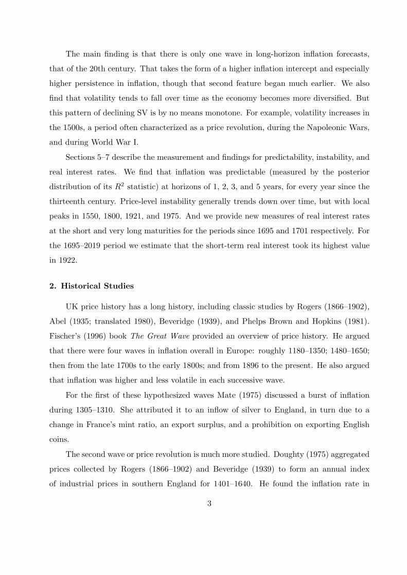
The main finding is that there is only one wave in long-horizon inflation forecasts,

that of the 20th century. That takes the form of a higher inflation intercept and especially

higher persistence in inflation, though that second feature began much earlier. We also

find that volatility tends to fall over time as the economy becomes more diversified. But

this pattern of declining SV is by no means monotone. For example, volatility increases in

the 1500s, a period often characterized as a price revolution, during the Napoleonic Wars,

and during World War I.

Sections 5–7 describe the measurement and findings for predictability, instability, and

real interest rates. We find that inflation was predictable (measured by the posterior

distribution of its R2 statistic) at horizons of 1, 2, 3, and 5 years, for every year since the

thirteenth century. Price-level instability generally trends down over time, but with local

peaks in 1550, 1800, 1921, and 1975. And we provide new measures of real interest rates

at the short and very long maturities for the periods since 1695 and 1701 respectively. For

the 1695–2019 period we estimate that the short-term real interest took its highest value

in 1922.

2. Historical Studies

UK price history has a long history, including classic studies by Rogers (1866–1902),

Abel (1935; translated 1980), Beveridge (1939), and Phelps Brown and Hopkins (1981).

Fischer’s (1996) book The Great Wave provided an overview of price history. He argued

that there were four waves in inflation overall in Europe: roughly 1180–1350; 1480–1650;

then from the late 1700s to the early 1800s; and from 1896 to the present. He also argued

that inflation was higher and less volatile in each successive wave.

For the first of these hypothesized waves Mate (1975) discussed a burst of inflation

during 1305–1310. She attributed it to an inflow of silver to England, in turn due to a

change in France’s mint ratio, an export surplus, and a prohibition on exporting English

coins.

The second wave or price revolution is much more studied. Doughty (1975) aggregated

prices collected by Rogers (1866–1902) and Beveridge (1939) to form an annual index

of industrial prices in southern England for 1401–1640. He found the inflation rate in

3

this index was particularly high during 1542–1560. Outhwaite (1982) used the indexes

constructed by Phelps Brown and Hopkins (1981) to suggest an increase in inflation began

around 1480 but certainly was clear by 1520.

Historians have long debated the causes of this inflation. Naturally a number of studies

focus on changes in the money supply. Gould (1970) described the debasement that began

in 1544, late in the reign of Henry VIII. Challis (1989) attributed the depreciation of the

currency beginning in 1521 to an increased supply of silver to the mint, often from the

crown itself (for example plate confiscated from monasteries). The debasements ended

with the Elizabethan restoration of the coinage in 1560–1561, but Outhwaite suggested

that inflation continued. Paper money was not introduced until late in the 17th century.

But foreign coins and tokens made of copper or lead were used to solve the problem of

small change (discussed by Sargent and Velde, 2003) in the Stuart period and so added to

the money supply.

The idea that silver from South America via Spain was the cause of inflation did not

become widespread until the 1600s. That idea was then popularized by Rogers (1866–1902)

and then of course by Earl Hamilton in his books on Spain published in the 1930s. Other

historians have emphasized physical explanations such as population changes, discussed by

Phelps Brown and Hopkins (1957) for the 1500s or by Fischer. But Outhwaite suggested

that data on both the money supply and population is unlikely to ever be refined enough

retrospectively to decide among explanations.

Braudel and Spooner (1967, p 400) studied the three-hundred-year span from 1450 to

1750 in Europe, noting that the consensus was:

The four long periods are: a fall, or rather stagnation, in the fifteenth century;a rise in the sixteenth continuing into the seventeenth century; then a fall untilabout 1720–50; finally a renewed inflation in the eighteenth century.

Fischer referred to the period from 1750 to 1820 as the third wave, with reference to

commodity prices and for England to the index of Phelps Brown and Hopkins (1957). The

British inflation of this period often is attributed to the suspension of gold convertibility

from 1797 to 1821. Braudel and Spooner (1967) focused on the long term (la longue duree,

to use the term of the Annales school), meaning the secular trend beyond cycles. We

suggest measuring this feature with a long-horizon inflation forecast.

4

3. Measurement

We use the annual retail price index, constructed and described by Clark (2020). After

1947 the price index is the series CDKO of the Office of National Statistics (ONS) and

applies to the entire UK. For 1870 to 1947 the source is from Feinstein (1995) again for

the UK. For 1209–1869 the locations are all in England. For simplicity we refer to the UK

in the paper’s title, following Clark (2020) and Thomas and Dimsdale (2017).

The largest component of the Clark price index is food, followed by fuel, lodging, light,

services, and manufactured goods. These in turn are aggregates of more detailed sub-

components. Clark describes how the weights vary over time to reflect changing patterns

of expenditure (especially after the Industrial Revolution) and also the absence of some

prices in the early centuries. Observations are missing from the Clark series for 1213,

1215, 1222, 1228–1231, 1234, and 1238–1244. As a result, our estimation and tests use

observations from 1245 on.

The upper panel of figure 1 shows this (log) price index. Here one can see the prolonged

inflation beginning in 1914. But the series also drifts up over 1245–1914. The lower panel

shows the corresponding inflation rate. The annual average inflation rate is 0.9% for the

entire span and 0.7% for the period before 1914. Appendix A discusses and graphs the

alternative indexes proposed by Allen (2001) and Thomas and Dimsdale (2017) as well as

the earlier indexes collected by Mitchell (1988).

One might wonder whether to statistically model the log price level (denoted pt) or,

instead, the inflation rate, πt. Table 1 shows augmented Dickey-Fuller tests statistics to

test for a unit root for each series. The statistics are calculated with four lags. The

results are shown first for four non-overlapping periods of the data (1245–1439, 1440–1633,

1634–1827, and 1828–2019), then for the periods before and after 1914, and finally for the

entire 1245–2019 sample. The findings can be summarized simply. There is evidence of a

unit root in the log price level but not in the inflation rate. This suggests modelling the

inflation rate as a stationary series over these spans.

Looking at the inflation rate in the lower panel of figure 1 then—so as to put the data

all on a similar, stationary scale and allow comparisons—shows that it is not easy to detect

patterns over time. High rates of inflation or deflation were common in earlier centuries:

5

It is really the persistence of inflation that seems to have changed. Equivalently, the lower

panel shows the noisiness in the early data, discussed in the introduction.

Historians therefore often have smoothed the commodity price or inflation rate series

by averaging. Figure 2 illustrates the effects for the Clark index. The three panels show

averages of the inflation rate over the 10, 20, and 30 years prior to each year. The sample

average is a random variable, so surrounding each average is a 68% confidence interval,

constructed with a HAC (Newey-West) standard error with 1, 2, or 3 lags. As the window

widens one can detect the waves discussed in section 2. The average was relatively high in

the late 1200s, middle 1500s, and early 1800s and particularly low in the late 1800s.

Our idea in this paper is to instead base the smoother on the model with the best fit

to the data or the best forecasts. This is in contrast to the averages in figure 2, which of

course use a pre-set window or span of years and fixed, equal weights on them. We test

for the number of lags needed to statistically explain inflation or forecast its future values

and we estimate the weights on those lags. And the weights are not fixed but may evolve

slowly over time. This time-variation allows us to study this long series in a unified way,

with no need for pre-set break dates or tests for structural breaks.

4. Time-Varying Autoregression

Our statistical framework is an AR(n) in inflation πt, with time-varing coefficients

and stochastic volatility (SV). The autoregression is given as follows:

πt = α0,t +n∑

i=1

αi,tπt−i + ξtǫt, ǫt ∼ N(0, 1)

(1)

while SV evolves as a (log squared) random walk:

ln ξ2t = ln ξ2t−1 + σφφt, φt ∼ N(0, 1

). (2)

The AR parameters are αi,t for i = 0, 1, 2, . . . , n. They follow a multivariate random

walk with possibly correlated innovations. Let αt ≡ α0,t, α1,t, α2,t, . . . , αn,t and ηt ≡

η0,t, η1,t, η2,t, . . . ηn,t. Then:

αt = αt−1 + ηt, ηt ∼ N(0n+1,Ωη). (3)

6

The innovations ηt to the multivariate random walk of the TVPs are not independent,

according to equation (3), because the covariance matrix Ωη is not restricted to be diagonal.

However, there is no correlation among either the elements of ηt and the innovation, ǫt, to

the AR(n), Eηℓ,tǫt

= 0, or the innovation to the (geometric) random walk, φt, of the

SV ξt, Eηℓ,tφt

= 0, ℓ = 0, 1, . . . , n. The same holds for φt and ǫt, E

φtǫt

= 0.

This time-series model has several appealing features. Using the recent history of

inflation as a basis for forecasts seems natural for economists and for historical forecasters.

But a AR with constant coefficients is unstable when fitted to this long span of data.

Imagine, then, fitting rolling ARs with a finite data window to track the evolution of a

forecasting equation. In that case one would need to choose the length of the widow over

which to estimate and any decay in the weights on observations within that span. The

TVP-SV-AR(n) automates these decisions, as weights on specific observations depend on

the Kalman gain, and observations in the distant past are gradually down-weighted through

the random walk structure in the coefficients. Our model allows for time-variation in the

scale of shocks to inflation and in their impact and persistence.

The TVP-SV-SVAR was introduced by Cogley and Sargent (2005) and Primiceri

(2005), who described a Markov chain Monte Carlo (MCMC) algorithm for estimation.

The code to run the Gibbs sampler is a univariate version of the algorithm described by

Canova and Perez Forero (2015). Their sampler uses the correction of Del Negro and

Primiceri (2015). We estimate SV in the TVP-AR(p)s by adapting our version of the

Canova and Perez Forero (2015) sampler to employ the ten-component mixture of normal

distributions developed by Omori, Chib, Shephard, and Nakajima (2007). Appendix B

describes our MCMC sampler in detail.

We estimate the TVP-SV-AR(n) on the Clark series for 1251–2019 while conditioning

on observations for 1245–1250, where n = 1, . . . , 6. These choices set the estimation

sample size to T = 769. Table 2 describes our priors for the TVP-SV-AR(n). Roughly

speaking these are empirical Bayes priors, based on OLS regression for the estimation

sample. Then table 3 describes how we select the autoregressive lag length, n. First, we

calculate log marginal data densities (MDDs), as recommended by Geweke (2005). This

criterion chooses the lag length n that fits the data best, in terms of its persistence and

7

volatility. The first row of table shows the data favor n = 3 conditional on our priors.

Second, we calculate the Bayesian version of the Akaike information criterion (IC).

Watanabe (2010) derives this IC and refers to it as the widely applicable information crite-

rion (WAIC). The WAIC chooses the lag length to yield the best one-year-ahead forecasts

(i.e. minimize predictive loss) along with estimating a penalty that approximates the

number of (unconstrained) parameters using information in the data and priors. Gelman

et al (2014, pp 173–174) label it the Watanbe-Akaike IC and recommend computing the

WAIC = −2[LTn − VT

n

], where LT

n is the posterior mean of the log predictive likelihood

of a TVP-SV-AR(n) and the penalty, VTn , is the posterior variance of this log likelihood.

The second row of table 3 indicates the WAIC chooses the lag length n = 5. Thus

the choice of TVP-SV-AR(n) depends on the question one is asking. Given our emphasis

on forecasting, we report and graph results from n = 5. Appendix C collects results for

n = 3, and comments on the differences, which are few.

We report on posterior densities for two types of forecasts. The changes in parameters

are unpredictable, so the long-horizon forecast is:

µπ,t ≡ limj→∞

Etπt+j =α0,t

1−∑n

i=1 αi,t

, (4)

which is computed as the median of the ratio of the posterior draws of the numerator to the

posterior draws of the denominator. This long-horizon forecast is the univariate version of

the inflation trend estimated and studied using a TVP-SV-VAR by Cogley and Sbordone

(2008).

The one-year-ahead forecast or measure of expected inflation is:

Etπt+1 = α0,t +n−1∑

i=0

αi+1,tπt−i. (5)

We report the median of the ensemble of one-year-ahead expected inflation. These forecasts

are created by running the Kalman filter on the posterior of a TVP-SV-AR(n) to produce

πt−i, i = 0, . . . , n−1, multiplying these predictions by the posterior draws of αi+1,t and

to the result adding the associated posterior draws of α0,t.

Figure 3 presents posterior moments of several hidden states. The upper left panel

contains the posterior median of the time-varying intercept, α0,t. The posterior median of

8

the sum of the lag TVPs,∑n

i=1 αi,t, is found in the upper right panel. This is a measure

of persistence. The lower left panel plots the median of the time-varying conditional mean

or long-horizon forecast µπ,t. SV is depicted in the lower right panel. The four panels also

display shadings that are 68 percent Bayesian credible sets (i.e., the 16 percent and 84

percent quantiles) of the TVPs and SV.

The key finding is in the lower left panel. Prior to 1914, the long-horizon forecasts

µπ,t do not vary significantly over time. One could draw a range of horizontal lines that

would pass through these credible sets. Thus a series of (non-independent) tests of the

hypothesis that each value was equal to this constant would not be rejected one-by-one.

Note that we are not arguing that the forecasts might be zero, though that hypothesis

also would not be rejected before 1914 except for the late 1200s. And we are of course

not arguing that the posterior density does not shift after 1914. We are arguing that the

long-run forecasts of inflation do not vary significantly over time before 1914.

The median long-run forecast (shown with the black line) does vary over time. It

is relatively high during the late 1200s and late 1500s, then slightly elevated during the

late 1700s and lower during the low-inflation and deflation epsiodes of the 1800s. So the

traditional waves discussed in sections 2 and 3 have not disappeared with this smoother.

We simply argue that they do not appear in the entire, 68% credible set.

The 20th-century wave in forecasts begins around 1914 and is associated with a rising

intercept and rising persistence. The median of µπ,t peaks in 1975. In that year the actual

inflation rate (shown in the lower panel of figure 1) also peaked, at 24.3%, the highest value

since the mid 1500s. That was also the year the Wilson government began its incomes

policy—described in the White Paper Attack on Inflation—and a year before the infamous

IMF loan to the UK. Subsequently the median declines steadily until 2019. The decline

features falls in the intercept and persistence measure. Median SV is also at an all-time

low at the end of this period.

There are three other noteworthy findings. First, the persistence measure—in the

upper right panel of figure 3—exhibits a very low frequency cycle. Its median falls until

1450–1500 then rises continuously until 1970 before falling slightly after that date. These

differences can be distinguished statistically. Thus it is not the case that the early inflation

9

data are simply so noisy that no patterns can be detected in them.

Second, the intercept term α0,t has considerable uncertainty. Its median follows the

historical wave pattern that then appears in the long-horizon forecast median. Then both

the median and the 68% credible set rise sharply in the 20th century. At that point, both

the rise in α0,t and the rise in∑n

i=1 αi,t contribute to the rise in µπ,t.

Third, median SV falls on average over time, so that feature is central to the speci-

fication. The decline in SV could be due to better measurement from more sources or to

genuine decreases in volatility with less dependence on weather and harvests. Either way,

though, that fall is not monotonic. For example, median SV rises from 1470 to 1550, during

the ‘price revolution’. That is one reason the increase in µπ,t is not sharper during that

period. Inflation rates were high in several years such as 1497 (18.1%), 1528 (32.6%), 1549

(21.4%), and 1550 (25.1%). But they also were volatile. For example there were deflations

in 1547 (-22.2%) and 1558 (-26.4%). Thus long-run forecasts were not revised sharply up.

Notice that median SV also rises during the Napoleonic Wars and during World War I.

Figure 4 shows the one-year-ahead forecasts for inflation (5) and associated forecast

errors from the TVP-SV-AR(n) with n = 5. It also shows 90% Bayesian credible sets.

With our focus on the very long run we have so far described the 20th century as a period

of inflation. But of course 1921–1934 was a period of deflation, as shown in figure 1. Such

fluctuations are one reason to adopt the TVP-SV-AR as opposed to one with constant

coefficients in a moving window for example: It can adapt to such changes in the data. It

is nevertheless not surprising that the forecast errors tend to mimic actual inflation during

the early 1920s. It would perhaps be difficult for any time-series model to predict the

sharp deflation of 1921–1923. The one-year-ahead forecasts tend to track actual inflation

with a lag, as one would expect of an AR. But it is noteworthy the long-horizon forecast

(shown in figure 3) does not fluctuate in response to this epsiode of deflation. The model

thus features a steepening of the term structure of inflation expectations as the posterior

density of Etπt+1 drops while that of µπ,t does not.

5. Predictability

To summarize the h-step-ahead predictability of inflation, we use the R2 statistic

10

proposed by Cogley, Primiceri, and Sargent (2010). This is 1 minus the ratio of the

conditional variance to the unconditional variance. It lies between 0 and 1. For example,

if the series is completely unpredictable then the conditional variance and unconditional

variances will coincide, their ratio will be 1, and R2 = 0. Also note that the statistics will

go to zero as h → ∞.

To see how this measure is computed, we need to write the TVP-SV-AR(n) in com-

panion (state space) form. Recall that ξt is the date-t, scalar SV of the AR(n). Define Πt

≡ [πt πt−1 . . . πt−n+1]′, A0,t ≡ [α0,t 0 . . . 0]

′, and Ξt ≡ [ξtǫt 0 . . . 0]

′. Label as At the

n× n companion matrix at date t of the AR(n), so that:

At ≡

α1,t α2,t . . . αn−1,t αn,t

1 0 . . . 0 00 1 . . . 0 0...

.... . .

......

0 0 . . . 1 0

. (6)

Then the TVP-SV-AR(n) can be written in companion form as:

Πt = A0,t +AtΠt−1 + Ξt. (7)

Define a selection vector s1 = [1 0 ... 0]1×n. The measure of predictability at horizon h is:

R2ht ≈ 1−

s1

[∑h−1j=0 Aj

tΩΞ,t

(Aj

t

)′]s′1

s1

[∑∞j=0 A

jtΩΞ,t

(Aj

t

)′]s′1

, (8)

where ΩΞ,t = ΞtΞ′t. In the denominator, the infinite sum

∑∞j=0 A

jtΩΞ,t(A

jt )

′ can be shown

to equal [In2 − (A′t ⊗A′

t)]−1

vec(ΩΞ,t) after reshaping this n2 column into a n× n matrix.

Let us define this n× n matrix as:

A∞,t = reshape([In2 − (At ⊗At)]

−1vec(ΩΞ,t), n, n

).

In the numerator, the finite sum is:

h−1∑

j=0

AjtΩΞ,t

(Aj

t

)′=

∞∑

j=0

AjtΩΞ,t

(Aj

t

)′−

∞∑

j=h

AjtΩΞ,t

(Aj

t

)′,

11

by adding and subtracting∑∞

j=h AjtΩΞ,t

(Aj

t

)′. Use the change of index j = ℓ + h, to

show:

∞∑

j=h

AjtΩΞ,t

(Aj

t

)′=

∞∑

ℓ=0

Aℓ+ht ΩΞ,t

(Aℓ+h

t

)′= Ah

t

[∞∑

ℓ=0

AℓtΩΞ,t

(Aℓ

t

)′](Ah

t

)′.

The implication is:

∞∑

j=0

AjtΩΞ,t

(Aj

t

)′−

∞∑

j=h

AjtΩΞ,t

(Aj

t

)′= A∞,t −Ah

t A∞,t

(Ah

t

)′.

The result is:

R2ht ≈ 1−

s1

[A∞,t −Ah

t A∞,t

(Ah

t

)′]s′1

s1A∞,ts′1

. (9)

Figure 5 shows the median R2ht statistics at horizons of 1, 2, 3, and 5 years, with their

68% credible sets. The first, and central, finding is this: There is predictability at each

horizon throughout the period. The credible sets do not include zero at any horizon and

date. Historical inflation in the lower panel of figure 1 appears very noisy, yet it exhibits

predictability in every year since the thirteenth century.

Second, median predictability at the 1-year horizon peaks at 0.44 in 1974. These

peaks are 0.23, 0.19, and 0.16 at the 2-, 3-, and 5-year horizons one year later. Third,

median predictability—like the median long-run forecast and median persistence in figure

3—falls over the last 45 years. But median predictability at the 1-year horizon remains

above 0.37. At the 2-, 3-, and 5-year horizons, median predictability is greater than 0.15,

0.13, and 0.10 during the last 45 years.

6. Price-Level Instability

Recall that pt denotes the log of the price level. We measure price-level uncertainty

at time t and horizon h, defined as the variance of acumulated inflation between t and

t + h: vart(pt+h − Etpt+h). Formulating this measure involves first computing expected

inflation and then finding the variance around that forecast. Price-level instability is then

12

defined—following Cogley and Sargent (2015) and Cogley, Sargent, and Surico (2015)—as

the total variation, and not just the unpredictable variation.

At horizon h, instability is given by the square root of the sum of the conditional

variance and the squared, conditional mean:

√vart (pt+h − Etpt+h) + (Etpt+h − pt)

2. (10)

The variance term is computed using the companion form of the TVP-SV-AR(5), which is

equation (7). It implies one-year ahead expected inflation is Etπt+1 = s1

[A0,t + AtΠt

],

where s1 = [1 0 . . . 0], Πt contains Kalman filtered predictions of Πt, and A0,t and At

represent draws from the posterior of the TVP-SV-AR(n).

The TVPs make computing j-year ahead expected inflation difficult. We invoke a

local approximation inspired by the anticipated utility model (AUM) of Kreps (1998) as

implemented by Cogley and Sbordone (1998) and Cogley, Primiceri, and Sargent (2010).

The local approximation holds A0,t and At at their current realizations to forecast inflation

j-years ahead, Etπt+j . The result is Etπt+j = s1[A0,t + Aj

t Πt

], where the operator Et·

conditions on the history of inflation, the TVPs, and SV through date t,(i.e., xt =

[xt xt−1 . . . x1], xt = πt, At, and ξt

), and the (hyper-)parameters Ωη and σφ.

We connect the equation generating Etπt+j and the conditional mean of accumulated

h-year ahead inflation as devised by Cogley, Sargent, and Surico (2015) in their equation

(9), though they use a different parametric model of inflation. The TVP-SV-AR(n) of

equations (1)–(3) turns the conditional mean into:

Et

pt+h − pt

= Et

h∑

j=1

πt+j = s1

[hA0,t +

h∑

j=1

Ajt Πt

]. (11)

Calculating the variance of the forecast error is more complicated. Appendix D contains

the details and formula for vart (pt+h − Etpt+h).

Figure 6 reports on the posterior density of the instability measures (10) by graphing

the median and 90% credible set at each year. We show results for n = 5 and at horizons

h =1, 2, 3, and 5. (Results for the uncertainty measure on its own are similar to those for

SV shown in the lower right panel of figure 3 and so are not shown separately.) Instability

13

behaves similarly over time at each horizon, but its value is greater at longer horizons, as

shown by the vertical axes in the four panels of figure 6.

Instability is high during the first 200 years of the sample, especially at horizons of 1

and 2 years. It then trends down over time, but there are four noteworthy local peaks at

each horizon. The first peak is in 1550, a year that saw an inflation rate of 25%. At this

time debasements continued during the reign of Edward VI until after Dudley replaced

Somerset as Protector in 1550. And in 1550 England was fighting expensive wars with

Scotland and France, that ended in 1551, while social unrest was widespread in southern

England. Note that there are several other high values for median instability during the

period of the Tudor debasements, particularly at horizons of 1 and 2 years.

The second peak is in 1800, during the War of the Second Coalition. In that year the

inflation rate was 22%, the highest level of the era, as seen in the lower panel of figure 1.

Next, at each horizon there are several elevated levels of median instability during World

War I and in the early 1920s, a period of whipsawing inflation. The third peak is in 1921,

the first of two years of very sharp deflation with π1921 = −9% and π1922 = −18% which

followed the tightening of monetary policy in 1920–1921. Howson (1973) described the

basis for the policy decisions of 1920.

The fourth peak is in 1975, a year that saw the peak inflation of the 1970s as dis-

cussed earlier. While this peak in price-level instability also coincides with a local peak in

uncertainty and SV, in this case there is a larger role for (Etpt+h − pt)2which also peaks

in 1975. As already noted, the mid 1970s was an extraordinary period in UK economic

history that saw the IMF loan and the government’s attempt to control inflation with wage

and price controls.

Of course we are modelling only inflation and could list events associated with any

year. By listing some events that coincided with these peaks in price-level instability we

are not implying that we necessarily understand their causes but rather leaving questions

for future research.

Cogley, Sargent, and Surico (2015) study UK inflation from 1791 to 2011 using the

unobserved components (UC) model of Stock and Watson (2007). Their model thus fea-

tures a stochastic trend in inflation in the form of an unobserved, random walk component.

14

It has two sources of SV, one in the permanent component and one in the transitory com-

ponent of inflation. It also has structural breaks in measurement error. Their model thus

is not directly comparable to ours. (And we found it difficult to identify the modern,

UC model for earlier centuries, given the lack of persistence in inflation rates we found in

figure 3 prior to 1800.) They also use the data assembled by Mitchell (1988) which display

higher and more volatile inflation rates during the Napoleonic Wars than do the Clark

data. Appendix A briefly describes the differences between these two series and graphs

them. And they report uncertainty and instability for horizons of 5 and 10 years.

Despite these differences in time span, model, data, and horizons, we nevertheless can

compare findings for the period after 1791. The two approaches have two key findings in

common. First, they both display local peaks in price-level instability in 1800, 1920, and

1975 at each horizon. Second, both studies find that the mid 1970s marked by far the

highest peak in price instability with a median rate 2–3 times higher than in 1800.

There are some differences in the findings though, both in peaks and troughs. First,

we find the second highest post-1791 peak in 1920 not in 1800, for each horizon. Overall

we find much more evidence of price instability in the early 1920s. Second, they find a

trough at around 1890 that is never matched in the twentieth century (by the median or

the inter-quartile range). Possibly because our data now run to 2019, we find that median

instability falls late in our sample to values comparable to those in the 1890s. We also find

relatively wide 90% credible sets late in our sample, though, which makes comparisons less

possible.

A final difference of course is that we can estimate price-level instability since the

1250s to put the values of the post-1791 period in context. Figure 6 shows that at horizons

of 1 or 2 years median instability peaked in the mid-1500s. At horizons of 3 or 4 years

though, the mid-1970s display the highest ever median values of price instability. Again,

though, there is considerable dispersion in these distributions throughout this span, so

that the 90% credible sets overlap when comparing these two periods.

7. Real Interest Rates

We next report implications for the history of real interest rates. We draw on the

15

expertise of Thomas and Dimsdale (2017) by using their series for nominal interest rates,

which begin in 1695. Thus our measures of real rates will differ from theirs only because

of the measurement of inflation expectations.

The nominal short rate is series M9 from Thomas and Dimsdale (2017): the annual

averages of Bank Rate 1695–1972, Minimum Lending Rate 1972–1981, Minimum Band 1

Dealing Rate 1981–1997, Repo Rate 1997–2006, and Bank Rate, 2006–2017. We update it

to 2019 from the Bank of England file baserates.xls. The long nominal interest rate is

series M10, the yield on perpetual annuities/consols. It connects for 1703–1726 yields on

new long-term issues, for 1727–1753 the yield on 3% perpetual annuities, for 1756–2015

the yield on Consols, and for 2016–2019 the 20-year zero coupon yield. These nominal

rates are shown in the top panels of figure 7.

Thomas and Dimsdale’s real short rate is based on NIESR inflation forecasts from

1959 and a range of measures from 1996 onwards. Prior to 1959 expectations are equal

to their realized value so the interest rate is an ex post one. Their measure of long-term

inflation expectations applies an HP filter to actual inflation with a parameter of 100 and

beginning in 1600. Notice also that their measure of inflation differs slightly from the Clark

measure, as documented in appendix A. We refer to these two real interest rates as the

Bank of England series.

Our measures of inflation expectations are from the TVP-SV-AR(5). From the nom-

inal interest rates we subtract the ensemble of values for the one-year ahead and long-

horizon inflation forecasts, then plot the median and the 90% credible set of these ex ante

real rates. In figure 7 the lower left panel shows the short-term real rates and the lower

right panel the long-term ones.

In comparing short-term, real interest rates in figure 7, note first that the Bank of

England series is much more volatile than ours, a fact that is not surprising since it is

an ex post series for much of the sample. Until the 1880s it often lies outside the 90%

credible set for our ex ante real interest rate. The two series coincide more closely after

that, except that the troughs in the Bank of England series are deeper than ours in the

early twentieth century. Both series reach their twentieth-century peak in 1922, following

the sharp monetary contraction of 1920–1921. In the Bank of England series comparably

16

high values occur in the 18th and 19th centuries. A striking difference, therefore, is that

for the TVP-SV-AR(5) 1922 marks the highest value for the entire 1695–2019 period. The

median, real short rate rises from -1.00% in 1920 to 10.49% in 1921 and 13.97% in 1922.

Long-term real rates are shown in the lower left panel of figure 7. It is interesting that

the median of our series peaks in 1974, at the same time as the nominal rate and before the

1990 peak in the Bank of England series. But there is more uncertainty associated with the

long-term real rate than the short-term real rate, and the Bank series lies within our 90%

credible set over the last 40 years. And of course there are other sources of information on

long-horizon inflation expectations for the late 20th century, including surveys and market-

based measures. Thus we emphasize earlier periods and those for which the differences

between the two series are the largest.

For the late 18th and early 19th centuries the Bank of England series is well below

our credible set, a pattern which is then reversed for several years after 1815. Our long-

horizon inflation forecasts do not react as much as the HP-filtered inflation series does to

the inflation during the Napoleonic Wars. Thus we do not estimate there to have been a

sharp fall then rise in the long-term real rate during the early decades of the 19th century.

A similar difference appears for the early 20th century. The inflation of World War I and

deflation of the 1920s lead to large swings in the Bank of England series that lie outside

our credible set, and our median estimate is smoother. In particular, the Bank of England

series is negative during both World Wars and again in the 1970s while our estimates of

the median, long-term real interest rate are not.

Borio, Disyatat, Juselius and Rungcharoenkitkul (2017) construct short-term and

long-term (10-year) real interest rates for the UK and other countries since 1870. They

form inflation expectations using an AR(1) model with a rolling 20-year window. For the

US, Lunsford and West (2019) construct short-term real rates for 1890–2016 by forecasting

inflation in the same way. For the 20th century these studies show a sawtooth pattern in

the real interest rate, as it trends down, then up, then down again. Figure 7 shows the

same pattern for our estimates of UK real rates at both maturities, concluding with very

low or negative estimates at the end of the sample.

These two studies just cited carefully examine a range of explanations for movements

17

in real interest rates. Our paper extends real interest rate measures back in time a further

175 years to 1695 and uses a TVP-SV-AR(5) to represent expected inflation, two features

that we hope will make the results useful in further studies of secular trends in real interest

rates.

8. Conclusion

We provide a statistical model that offers a window on the work of economic historians

—principally Clark (2020)—who have assembled price indexes for the UK (and earlier

England) since the thirteenth century. The TVP-SV-AR model produces forecasts for

inflation using a single model for the entire period, with slowly-evolving parameters and

no need for structural break tests.

A central finding is that there is a single, Hokusai-scale wave in historical, long-horizon

inflation forecasts, occurring in the 20th century. We also find a gradual rise in inflation

persistence over time, and a tendency for stochastic volatility in inflation to fall. Despite

the noisiness that seems apparent in historical inflation, inflation is predictable at horizons

of 1, 2, 3 and 5 years for each year since 1251, as measured by the R2 statistic. Price-

level instability tends to decline over time, which puts the instability of the mid 1970s in

historical context. But there are notable, local peaks in median estimates of instability

in 1550, 1800, 1921, and 1975. For the 1695–2019 period we estimate that a distinct,

overall peak in the short-term real interest rate ocurred in 1922, following the monetary

contractions of 1920–1921.

18

References

Abel, Wilhelm (1980) Agricultural fluctuations in Europe from the thirteenth to the twen-

tieth centuries. London: St. Martin’s Press. Translated by Olive Ordish fromAgrarkrisen und Agrarkonjunktur in Mittel Europa vom 13 bis zum 19 Jahrhundert

(Berlin, 1935; new eds. 1966, 1978).

Allen, Robert C. (2001) The great divergence in European wages and prices from themiddle ages to the First World War. Explorations in Economic History 38, 411–447.

Beveridge, William (1939) Prices and Wages in England from the Twelfth to the Nineteenth

Century. New York: Longmans, Green and Company.

Borio, Claudio, Piti Disyatat, Mikael Juselius and Phurichai Rungcharoenkitkul (2017)Why so low for so long? A long-term view of real interest rates. BIS working paperNo. 685.

Braudel, Fernand P. and Frank Spooner (1967) Prices in Europe from 1450 to 1750. The

Cambridge Economic History of Europe 4, 378–486.

Canova, Fabio and Fernando J. Perez Forero (2015) Estimating overidentified, nonrecur-sive, time-varying coefficients structural vector autoregressions. Quantitative Eco-

nomics 6, 359–384.

Carter, Christopher K. and Robert Kohn (1994) On Gibbs sampling for state space models.Biometrika 81, 541–553.

Challis, Christopher E. (1989) Currency and the economy in Tudor and early Stuart Eng-

land. London: The Historical Association.

Clark, Gregory (2020) What Were the British Earnings and Prices Then? (New Series)MeasuringWorth, 2020. URL: www.measuringworth.com/ukearncpi/

Cogley, Timothy, Giorgio Primiceri, and Thomas J. Sargent (2010) Inflation-gap persis-tence in the U.S. American Economic Journal: Macroeconomics 2, 43–69.

Cogley, Timothy and Thomas J. Sargent (2005) Drifts and volatilities: Monetary policiesand outcomes in the post WWII U.S. Review of Economic Dynamics 8, 262–302.

Cogley, Timothy and Thomas J. Sargent (2015) Measuring price-level uncertainty andinstability in the United States, 1850–2012. Review of Economics and Statistics 97,827–838.

Cogley, Timothy, Thomas J. Sargent, and Paolo Surico (2015) Price-level uncertainty andinstability in the United Kingdom. Journal of Economic Dynamics & Control 52,1–16.

Cogley, Timothy, and Argia M. Sbordone (2008) Trend inflation, indexation, and inflationpersistence in the New Keynesian Phillips curve. American Economic Review 98,2101–2126.

19

Crafts, Nicholas F.R. and Terence C. Mills (1994) Trends in real wages in Britain, 1750–1913. Explorations in Economics History 31, 176–194.

del Negro, Marco and Giorgio E. Primiceri (2015) Time varying structural vector autore-gressions and monetary policy: A corrigendum. Review of Economic Studies 82,1342–1345.

Doughty, Robert A. (1975) Industrial prices and inflation in southern England, 1401–1640.Explorations in Economic History 12, 177–192.

Faust, Jon and Jonathan H. Wright (2013) Forecasting inflation. Chapter 1 in GrahamElliott and Allan Timmermann eds. Handbook of Economic Forecasting, volume 2A.Amsterdam: Elsevier.

Feinstein, Charles H. (1991) A new look at the cost of living. In Foreman-Peck, J, ed. NewPerspectives on the Late Victorian Economy, Cambridge University Press.

Feinstein, Charles H. (1995) Changes in nominal wages, the cost of living and real wagesin the United Kingdom over two centuries. In P Scholliers and V. Zamagni (eds.),Labour’s Reward: Real Wages and Economic Change in 19th- and 20th-Century Eu-

rope. Aldershot, Hants: Edward Elgar.

Feinstein, Charles H. (1998) Pessimism perpetuated: Real wages and the standard of livingin Britain during and after the Industrial Revolution, Journal of Economic History

58, 625–658.

Fischer, David Hackett (1996) The Great Wave: Price Revolutions and the Rhythm of

History. Oxford University Press.

Gelman, Andrew, John B. Carlin, Hal S. Stern, David B. Dunsun, Aki Vehtari, and Don-ald B. Rubin (2014) Bayesian Data Analysis (third edition). CRC Press, Taylor &Francis Group: New York, NY.

Geweke, John (2005) Contemporary Bayesian Econometrics and Statistics. New York:Wiley.

Gould, J.D. (1970) The Great Debasement. Oxford University Press.

Harvey, Andrew, Esther Ruiz, and Neil Shephard (1994) Multivariate stochastic variancemodels. Review of Economic Studies 61, 247–264.

Howson, Susan (1973) “A dear money man”?: Keynes on monetary policy, 1920. Economic

Journal 83, 456–464.

Koop, Gary, and Simon Potter (2011) Time varying VARs with inequality restrictions.Journal of Economic Dynamics & Control 35, 1126–1138.

Kreps, David (1998) Anticipated utility and dynamic choice, In Frontiers of Research in

Economic Theory: The Nancy L. Schwartz Memorial Lectures, 1983–1997. Jacobs,Donald P., Ehud Kalai, Morton I. Kamien, and Nancy L. Schwartz (eds.), 242–274,Cambridge, UK: Cambridge University Press.

20

Lunsford, Kurt G. and Kenneth D. West (2019) Some evidence on secular drivers of USsafe real rates. American Economic Journal Macroeconomics 11(4), 113–139.

Mate, Mavis (1975) High prices in early fourteenth-century England: Causes and conse-quences. Economic History Review 28, 1–16.

Mitchell, Brian R. (1988) British Historical Statistics. Cambridge University Press.

O’Donoghue Jim, Louise Goulding, and Grahame Allen (2004) Consumer price inflationsince 1750, ONS Economic Trends 604, March 2004.

Omori, Yasuhiro, Siddhartha Chib, Neil Shephard, and Jouchi Nakajima (2007) Stochasticvolatility with leverage: Fast and efficient likelihood inference. Journal of Economet-

rics 140, 425–449.

Outhwaite, R. B. (1982) Inflation in Tudor and early Stuart England. 2nd ed. London:Macmillan.

Phelps Brown, Henry and Sheila V. Hopkins (1957) Wage-rates and prices: Evidence forpopulation pressure in the sixteenth century. Economica 24, 289–306.

Phelps Brown, Henry and Sheila V. Hopkins (1981) A Perspective of Wages and Prices.

London: Methuen.

Primiceri, Giorgio E. (2005) Time varying structural vector autoregressions and monetarypolicy. Review of Economic Studies 72, 821–852.

Rogers, James E. Thorold (1866–1902) A History of Agriculture and Prices in England from

the Year after the Oxford Parliament, 1259, to the Commencement of the Continental

War, 1793., Oxford: Clarendon Press.

Sargent, Thomas J. and Francois R. Velde (2003) The Big Problem of Small Change.

Princeton, NJ: Princeton University Press.

Stock James H. and Mark W. Watson (2007) Why has US inflation become harder toforecast? Journal of Money, Credit and Banking 39(S1), 3–33.

Thomas, Ryland and Nicholas Dimsdale (2017) A millennium of UK data. Bank of EnglandOBRA datset:bankofengland.co.uk/research/Pages/onebank/threecenturies.aspx

Watanabe, Sumio (2010) Asymptotic equivalence of Bayes cross validation and WidelyApplicable Information Criterion in singular learning theory. Journal of Machine

Learning Research 11, 3571–3594.

21

Table 1. Augmented Dickey-Fuller Tests

Time Period πt pt

1245–1439 -8.85*** -2.83*

1440–1633 -8.02*** 0.58

1634–1827 -6.64*** -0.64

1828–2019 -3.64*** 1.35

1245–1913 -15.02*** -0.78

1914–2019 -3.25** 0.56

1245–2019 -11.96*** 4.18

Notes: The table shows augmented Dickey-Fuller test statistics for a unit root in the inflation rate πt and

the log price level pt for each quarter of the sample, for subsamples before and after 1914, and for the entire

sample. The lag length is 4. Asymptotic critical values at the 10%, 5%, and 1% levels are -2.57, -2.87,

and -3.44, respectively. The Dickey-Fuller tests and critical values are obtained using the RATS-Estima

procedure dfunit.src. The middle column of the table reports *** to denote significance at the 1% level,

** at the 5% level and * at the 10% level. There is evidence of a unit root in the price level but not in

the inflation rate, which supports modelling the inflation rate as a stationary series over these long spans

of annual data.

22

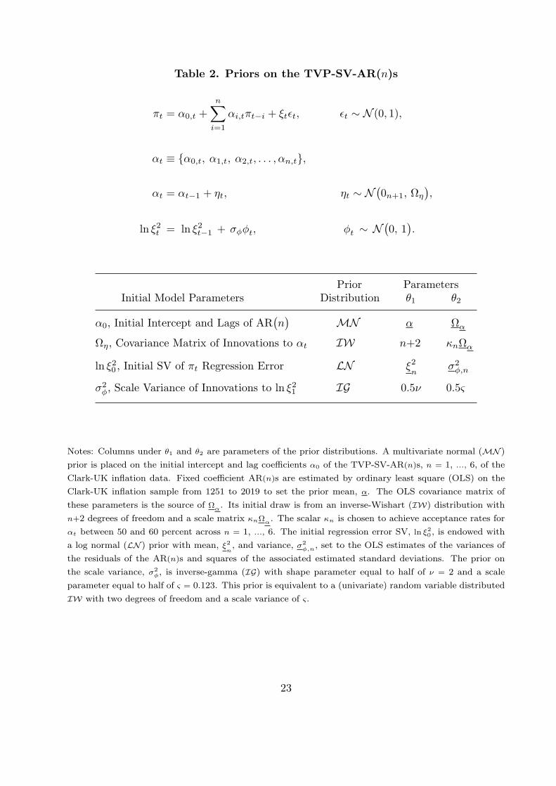
Table 2. Priors on the TVP-SV-AR(n)s

πt = α0,t +n∑

i=1

αi,tπt−i + ξtǫt, ǫt ∼ N (0, 1),

αt ≡ α0,t, α1,t, α2,t, . . . , αn,t,

αt = αt−1 + ηt, ηt ∼ N(0n+1, Ωη

),

ln ξ2t = ln ξ2t−1 + σφφt, φt ∼ N(0, 1

).

Prior ParametersInitial Model Parameters Distribution θ1 θ2

α0, Initial Intercept and Lags of AR(n)

MN α Ωα

Ωη, Covariance Matrix of Innovations to αt IW n+2 κnΩα

ln ξ20 , Initial SV of πt Regression Error LN ξ2n

σ2φ,n

σ2φ, Scale Variance of Innovations to ln ξ21 IG 0.5ν 0.5ς

Notes: Columns under θ1 and θ2 are parameters of the prior distributions. A multivariate normal (MN )

prior is placed on the initial intercept and lag coefficients α0 of the TVP-SV-AR(n)s, n = 1, ..., 6, of the

Clark-UK inflation data. Fixed coefficient AR(n)s are estimated by ordinary least square (OLS) on the

Clark-UK inflation sample from 1251 to 2019 to set the prior mean, α. The OLS covariance matrix of

these parameters is the source of Ωα. Its initial draw is from an inverse-Wishart (IW) distribution with

n+2 degrees of freedom and a scale matrix κnΩα. The scalar κn is chosen to achieve acceptance rates for

αt between 50 and 60 percent across n = 1, ..., 6. The initial regression error SV, ln ξ20, is endowed with

a log normal (LN ) prior with mean, ξ2n, and variance, σ2

φ,n, set to the OLS estimates of the variances of

the residuals of the AR(n)s and squares of the associated estimated standard deviations. The prior on

the scale variance, σ2

φ, is inverse-gamma (IG) with shape parameter equal to half of ν = 2 and a scale

parameter equal to half of ς = 0.123. This prior is equivalent to a (univariate) random variable distributed

IW with two degrees of freedom and a scale variance of ς.

23

Table 3. Evaluation of Fit of the TVP-SV-AR(n)s

AR(1) AR(2) AR(3) AR(4) AR(5) AR(6)

ln MDD 749.20 754.36 783.40 756.50 775.37 764.46

WAIC -561.62 -667.04 -677.91 -693.51 -694.83 -693.50

Notes: The first row contains log marginal data densities, ln MDDs, of the TVP-SV-AR(n)s. The modi-

fied harmonic mean estimator of Geweke (2005) is employed to calculate the MDDs. The MDDs represent

evidence the data have about the TVP-SV-AR(n)s. The second row reports the Widely Applicable Infor-

mation Criterion (WAIC) developed by Watanabe (2010). The WAIC, also referred to as the Watanabe-

Akaike-IC, is an estimate of the predictive loss of a TVP-SV-AR(n). This notion of predictive loss equals

twice the difference between the sum of the posterior variances of the log predictive likelihoods and the

mean of the log predictive likelihoods following the advice of Gelman et al (2014). Estimates of the like-

lihoods are obtained from the predictive steps of the Kalman filter, which are also needed to compute

the MDDs. The sum of the posterior variances is an estimate of the effective dimension of the parameter

vector of the TVP-SV-AR(n)s, which serves as the penalty term of the WAIC.

24

Figure 1: The Clark-UK Price Level and Inflation, 1251–2019

Notes: The top panel display the natural log of the Clark-UK price level, pt = ln(

Pt/

100)

. The bottom panel plots the inflation rate of

Clark-UK price series, pt − pt−1.

25

Figure 2: Ten-, Twenty-, and Thirty-Year Moving Averages of Clark-UK Inflation

Notes: The top panel contains the 10-year moving average (MA) of UK inflation, π10,t , from 1254 to 2019 surrounded by shadings that

are 68% Newey-West confidence bands computed with one lag. Two lags are used to construct the 68% Newey-West confidence bands

of the 20-year MA of UK inflation, π20,t , that runs from 1264 to 2019 and appear in the middle panel. The 30-year MA of UK inflation,

π30,t , runs 1274 to 2019, are displayed in the bottom panel and relies on three lags to calculate 68% Newey-West confidence bands.

26

Figure 3: Posterior Moments of the TVP-SV-AR(5) on Clark-UK Inflation, 1251–2019

Notes: The top left panel contains the posterior median of the time-varying intercept, α0,t . The posterior median of the sum of the lag

TVPs,∑5ℓ=1αℓ,t , is found in the top right panel. A plot of the time-varying conditional mean of Clark-UK inflation is depicted in the

bottom left panel as the posterior median of µπ,t = α0,t

/(

1−∑5ℓ=1αℓ,t

)

. The SV of Clark-UK inflation is displayed in the bottom right

panel. The four panels also display shadings that are 68% Bayesian credible sets (i.e., 16% and 84% quantiles) of the TVPs and SV.

27

Figure 4: 1-Year Ahead Expected Clark-UK Inflation and Its Ex Post Forecast Error, 1251–2019

Notes: The top panel plots median 1-year ahead expected Clark-UK Inflation, Etπt+1. Expected inflation is estimated using the Kalman

filter, sample Clark-UK inflation, and the posterior distribution of the TVP-SV-AR(

5)

. The bottom panel contains the ex post forecast

error, πt+1 − Etπt+1. The panels also contain shadings that are 90% Bayesian credible sets (i.e., 5% and 95% quantiles).

28

Figure 5: Predictability of Clark-UK Inflation 1-, 2-, 3-, and 5-Years Ahead, 1251–2019

Notes: The top left panel plots the median 1-year ahead R-square statistic, R21t , which is computed as described in equation

(

8)

, from

1251 to 2019. The shadings around R21t are 68% Bayesian uncertainty bands. Similarly, median R2

2t , R23t , and R2

5t appear in the top

right, bottom left, and bottom right panels along with 68% Bayesian uncertainty bands as the shadings. The R-square statistics are

computed using the posterior distribution of the TVP-SV-AR(

5)

.

29

Figure 6: Price-Level (In)Stability of Clark-UK Series, 1251–2019

Notes: The top left panel plots the median of the 1-year ahead square root of the sum of the conditional variance and the squared,

conditional mean,

√

vart(

pt+1 − Etpt+1

)

+

(

Etpt+1 − pt)2

, from 1251 to 2019. The shadings around this statistic are 90% Bayesian

uncertainty bands. The median 2-, 3-, and 5-year ahead price-level stability statistics are displayed in the top right, bottom left, and

bottom right panels along with shadings that are 90% Bayesian uncertainty bands. The price-level stability statistics are computed

using the posterior distribution of the TVP-SV-AR(

5)

.

30

Figure 7: UK Nominal and Real Short- and Long-Term Interest Rates

Notes: The top row plots UK nominal short- and long-term interest rates; see section 7 and the appendix for details. The bottom row

depicts ex ante short- and long-term real rates, rNS,i,t = RBofE,i,t − Etπt+1, in the left and right panels, where i = S(short) and L(long).

Short-term (long-term) rates begin in 1695 (1703) and end in 2019. One-year ahead expected inflation is computed using the posterior

distribution of the TVP-SV-AR(

5)

. In the bottom row of panels, the shadings are 90% Bayesian uncertainty bands.

31

Appendix A: Alternative Price Indexes

An alternative to the Clark index is the Bank of England CPI series assembled by

Thomas and Dimsdale (2017). Prior to 1661 it uses a slightly different version of the Clark

index that applies to the poorest workers and excludes services. It uses the Schumpeter-

Gilboy index from Mitchell (1988) for 1661–1750, the series from Crafts and Mills (1991)

for 1750–1770, the series from Feinstein (1998) for 1770–1882, the series from Feinstein

(1991) for 1882–1914, the series from the ONS (O’Donoghue, Goulding, and Allen, 2004)

for 1914–1949, and the CPI (ONS) for 1949–2016. There are 807 observations in this series

up to 2016.

Allen (2001) constructed a city-level CPI for London and for a large number of other

European cities. They are Laspeyres indexes using what he describes as a ‘pre-modern

basket’ (given in his table 3). The basket differs across cities depending on the local

food and fuel sources. As is usual with early price indexes, the data sources tend to be

institutions such as hospitals or schools but one of Allen’s many contributions is to use

retail bread prices rather than grain prices. For London the Allen series spans 1264–1913

or 649 observations. Allen notes that his London index closely tracks that of Feinstein

(1998) when they overlap. There does not appear to be a London-level CPI after 1913 to

which to splice this series.

The Allen and Clark series differ in several respects: (i) Clark uses data from through-

out England and later the UK while Allen applies to London; (ii) Allen omits lodging

(though for the early period this was a relatively small share of expenditure), manufac-

tures such as tools, and services; (iii) Clark’s weights change over time; (iv) both series

use bread rather than grain but they estimate the retail bread price in different ways.

Figure A1 shows the logs of the Clark series (in blue), the Bank of England series (in

red, dashed), and the Allen series (in green, dotted) for four periods each of roughly two

centuries: 1209–1399; 1400–1599; 1600–1799; and 1800–2019. The Bank of England series

is rescaled so that 2010 = 100 as for the Clark series. The Allen series is rescaled so that

it is equal to the Clark series when it ends in 1913. The Bank of England series and the

Allen series are more volatile than the Clark series, perhaps because of the categories of

consumption spending that they omit.

32

Cogley, Sargent, and Surico (2015) use a price index found in Mitchell (1988). He

spliced together indexes from Lindert and Williamson for 1781–1846 and from Bowley for

1846–1914. We rescale the Mitchell series so that it is equal to the Clark series in 1913.

Figure A2 then graphs the log price level from Clark (in blue, as above) and Mitchell (in

red, dashed) for 1781–1947. Two obvious differences are in the 1946–1947 inflation rates

and particularly in the greater volatility of the Lindert-Williamson and Bowley inflation

rate series compared to the Clark series. We claim no expertise in deciding which is the

best index, but simply note that the greater volatility of the early Mitchell series seems due

to the Lindert-Williamson data. This volatility is not evident in more recently constructed

series such as those of Clark or the Bank of England. In the Clark data we also do not have

the discrete breaks in the series source that allow Cogley, Sargent, and Surico to identify

measurement error as distinct from SV in gap inflation. For both reasons we do not model

measurement error as those authors did, and instead rely on having access to more recent

sources by Clark, Crafts and Mills, Feinstein, and others.

33

Figure A1: The Clark-, Bank of England-, and Allen-UK Price Levels on Several Subsamples

Notes: The panels depict the natural logs of the Clark-, Bank of England-, and Allen-UK price levels, pt = ln(

Pt/

100)

. The top right,

top left, bottom left, and bottom right panels plots these price levels from 1209 to 1399, 1400 to 1599, 1600 to 1799, and 1800 to

2019. The samples of the Clark-, Bank of England-, and Allen-UK price data run from 1208 to 2019, 1208 to 2016, and 1263 to 1913,

respectively. The Bank of England price level is rescaled for it to equal 100 in 2010 as is the Clark series. The Allen series is rescaled

to force its last observation in 1913 to equal the Clark series at that date.

34

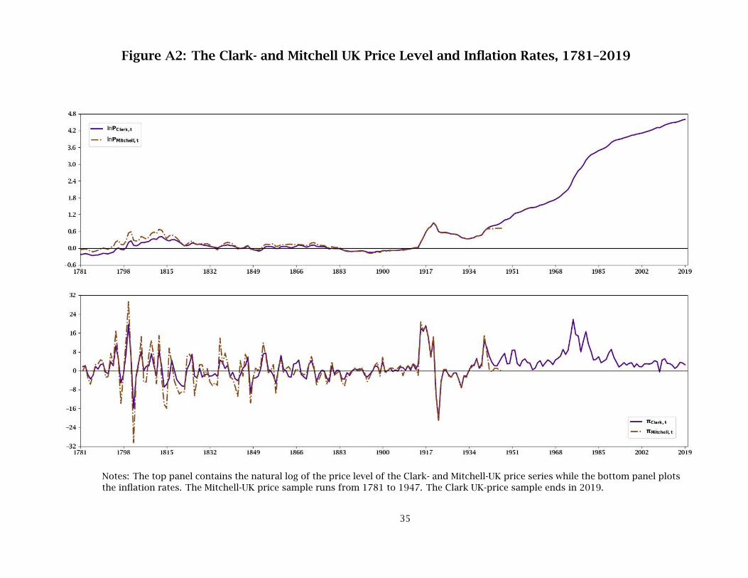
Figure A2: The Clark- and Mitchell UK Price Level and Inflation Rates, 1781–2019

Notes: The top panel contains the natural log of the price level of the Clark- and Mitchell-UK price series while the bottom panel plots

the inflation rates. The Mitchell-UK price sample runs from 1781 to 1947. The Clark UK-price sample ends in 2019.

35

Appendix B: A Gibbs MCMC Sampler for a TVP-SV-AR(n)

This appendix discusses the Gibbs MCMC sampler that draws from the posterior of

a AR(n)with TVPs and an innovation subject to SV. We reproduce the AR

(n)and its

TVPs and SV as state variables here:

πt = α0,t +

n∑

i=1

αi,tπt−i + ξtǫt, ǫt ∼ N(0, 1

), (1)

ln ξ2t = ln ξ2t−1 + σφφt, φt ∼ N(0, 1

), (2)

αt = αt−1 + ηt, ηt ∼ N(0n+1, Ωη

). (3)

The AR(n)of equation (1) is linear in the time-varying intercept, α0,t, and lag co-

efficients, α1,t, . . . , αn,t, but nonlinear in the Gaussian innovation ǫt that is hit by SV in

the form of ξt. Its square evolves as the geometric random walk (2) in the innovation φt

that is scaled by the static volatility σφ. Equation (3) is the multivariate random walk

generating updates of the time-varying intercept, α0,t, and lag coefficients αi,t, where αt

≡[α0,t α1,t α2,t . . . αn,t

]′and ηt ≡

[η0,t η1,t η2,t . . . ηn,t

]′. Since the covariance matrix

Ωη is unrestricted, the multivariate random walk (3) yields TVPs that can be correlated.

This is not true of the elements of ηt and ǫt and ηt and φt because Eηℓ,tφt

= E

ηℓ,tǫt

= 0, ℓ = 0, 1, . . . , n. A similar restriction is imposed on φt and ǫt, Eφtǫt

= 0.

The Gibbs MCMC sampler rests on the Canova and Perez Forero (2015) implemen-

tation of the Del Negro and Primiceri (2015) algorithm. This algorithm constructs the

posterior of a state space model with SV in the observation equations. Canova and Perez

Forero (2015) apply this algorithm to sample from the posterior of a structural VAR with

TVPs and SV. We modify the instructions found in Canova and Perez Forero (2015) to

sample from the TVP-SV-AR(n)of equations (1), (2), and (3). The TVP-SV-AR

(n)can

be cast as a state space model in which the observation is equation (1) and the states are

generated by the random walks of equations (2) and (3). Our Gibbs MCMC sampler ex-

ploits this state space representation to create posterior draws of αt and Ωη using Kalman

filtering and Kalman smoothing similar to the way Canova and Perez Forero (2015) build

36

on the insights of Carter and Kohn (1994) for Gibbs sampling. Similar Kalman filtering

and smoothing routines are employed to make posterior draws of ln ξ2t and σ2φ subsequent

to determining the volatility state st. Drawing st depends on results in Harvey, Ruiz, and

Shephard (1994) and Omori, Chib, Shephard, and Nakajima (2007).

A brief sketch of our changes to the sampler of Canova and Perez Forero (2015)

clarifies the conditioning needed to draw from the posterior of the TVP-SV-AR(n). Begin

by drawing αT conditional on πT and the current draws of Ωη, ST , ξT , and σ2

φ, where, for

example, ST =[s1 s2 . . . st . . . sT

]′. As in Canova and Perez Forero (2015), we adopt the

advice of Koop and Potter (2011) to test whether any αt in αT =[α1 α2 . . . αt . . . αT

]′

is explosive by calculating the eigenvalues of the companion matrix:

At ≡

α1,t α2,t . . . αn−1,t αn,t

1 0 . . . 0 00 1 . . . 0 0...

.... . .

......

0 0 . . . 1 0

.

If the largest eigenvalue is greater than one, the proposed draw of αT is tossed out and

the sampler adds another instance of the previous draw to the posterior. Otherwise, the

proposed αT is retained as the updated draw. In either case, the draw is used to update

Ωη, given the current draws of ST , ξT , and σ2φ. Note that a non-diagonal Ωη is consistent

with the multi-move sampler of Carter and Kohn (1994). Next, ST is drawn, given πT ,

updates of αT and Ωη and the current draws of ξT and σ2φ. This is followed by drawing ξT

conditional on πT , updates of αT , Ωη, and ST , and the current draw of σ2φ. Finally, draw

σ2φ conditional on πT and the updates of αT , Ωη, ST , and ξT . We repeat these steps to

obtain M draws from the posterior of the TVP-SV-AR(n).

The following algorithm has details about our Gibbs MCMC sampler, where the pre-

vious posterior draws at the start of step m are ~αTm−1,

~Ωη,m−1, ln ~ξ 2Tm−1, and ~σ 2

φ,m−1.

1. Running the Kalman filter generatesαt|t

Tt=1

and its mean square error (MSE),Γα,t|t

Tt=1

, given the initial conditional α0|0 that is drawn according to the prior listed

in table 2.

37

2. Draw αT |T ∼ N(αT |T , Γα,T |T

), which is input into the Kalman smoother to generate

αT−1|T ∼ N(αT−1|T , ΓT−1|T

), continue iterating the Kalman smoother backwards in

time in this way to create the smoothed candidate draw αT =αt|T

Tt=1

, where αt|T

and Γα,t|T are outputs of the smoothing operations.

3. Employ αT to form AT , which if any companion matrix has an eigenvalue greater than

one, discard αT and keep the previous draw ~αTm−1. Otherwise, update the posterior to

~αTm = αT .

4. Compute the empirical moment matrix of ~αTm, Ωα,m, to draw the update of Ωη, which

is ~Ωη,m ∼ IW(Ω+ Ωα,m, T + n+ 1

).

5. Since ǫt is Gaussian, draw st from the 10-component mixture of Omori, Chib, Shephard,

and Nakajima (2007).

6. Given ~ST = ~stTt=1 and ln ξ20|0, which is drawn using the prior shown in table 2,

generateln ξ2

t|t

T

t=1and its MSE,

Γξ,t|t

Tt=1

, using the Kalman filter.

7. Running the Kalman smoother backwards from date T creates ~ξ T =ln ~ξ 2

t|T

T

t=1by

first drawing ln ~ξ 2T |T ∼ N

(ln ξ2

T |T , Γξ,T |T

)that in turn aids in producing ln ξ 2

t|T and

Γξ,t|T to sample ln ~ξ 2t|T ∼ N

(ln ξ 2

t|T , Γξ,t|T

), t = T−1, . . . , 1.

8. Draw ~σ 2φ,m ∼ IG

(0.5 (ν + T ) , 0.5

(ς + σ2

φ,m

)), where ν and ς are the degrees of free-

dom and variance of the prior on σ2φ described in table 2 and σ2

φ,m is the empirical

moment matrix of ~ξ T .

9. Repeat steps 1 to 8 to obtain M draws, where m = 1, . . . , M.

Additional information is needed to construct the posterior of a TVP-SV-AR(n)by

running the Gibbs MCMC sampler. The Gibbs MCMC sampler calibrates κn to yield an

acceptance rate for~αTm

Mm=1

of between 50 and 60%. Hence, the calibration of κn depends

on the lag length n = 1, . . . , 6. Sampling ~ST and ~ξ T relies on rewriting the TVP-SV-AR(n)

as ~Yt ≡ πt − ~α0,t −∑k

i=1 ~αi,tπt−i = ξtǫt, passing the natural log through gives ln ~Y2t =

2 ln ξt + ln ǫ2t , and the approximation ln(~Y 2t + ι

)≈ 2 ln ξt + ln ǫ2t , where ι = 0.0001 to

ensure the term inside the log on the left of the approximation is bounded away from zero.

38

Harvey, Ruiz, and Shephard (1994) brought attention to the fact that the log of the square

of a Gaussian random deviate is distributed ln ǫ2t ∼ lnχ2(1)with a mean of −1.2704 and

a variance equal to 3.14162/2. Omori, Chib, Shephard, and Nakajima (2007) approximate

lnχ2(1)using these facts and a 10-component mixture of normal distributions, which is

our source for drawing ~ST . We generate a burn-in of 0.5M = 250,000 steps from the Gibbs

MCMC sampler, create M posterior draws, and report results for a TVP-SV-AR(n)on

a thinned posterior by sampling without replacement D = 2000 draws of the integers m

= 1, . . . , M. These draws are used to pull D realizations from the entire ensemble of M

posterior draws of a TVP-SV-AR(n).

The Gibbs MCMC sampler is run using Julia v.1.5.2. The same statistical and

computational software is employed to calculate the log MDDs, the WAICs, and the R2ht

and price stability statistics. The econometric software package RATS by Estima is used

to construct the unit root tests in table 1 and the MA and Newey-West confidence bands

displayed in figure 2. The figures are constructed using the Julia packages PyPlot and

PyCall to engage the Python package Matplotlib v3.3.4.

39

Appendix C: Results for TVP-SV-AR(3)

This appendix collects figures for the TVP-SV-AR(3) model. The figures are num-

bered to allow comparison with those in the text. Thus we begin with figure C3 which is

in the same format as figure 3, but uses lag length n = 3 instead of n = 5.

Figure C3 shows features of the posterior densities for the hidden states. The findings

are similar to those in figure 3 in several respects. No waves in µπ,t are apparent until

the 20th century. Again the peak is in 1975. Persistence falls until roughly 1500 then

rises until the 1970s. Median SV trends down, but it fluctuates. However, there are also

two differences. First, the top right panel shows that the model with n = 3 suggests less

negative serial correlation before 1900 and less persistence after 1900. Second, the lower

left panel of figure C3 shows a peak in the median of µπ,t of about 6% in 1975 whereas the

peak for n = 5 was 4.5%.

Figure C4 shows the one-year ahead forecasts for inflation (5) and associated forecast

errors. The results are quite similar to those shown for n = 5 in figure 4.

Figure C5 shows the median R2ht predictability statistics, with their 68% credible sets.

This figure shows somewhat greater uncertainty about predictability (wider 68% credible

sets) at each horizon, compared with the TVP-SV-AR(5). Another noteworthy difference

is that the AR(3)-produced median predictability rises at each horizon at the end of the

sample, though it is still below its peak in the 1970s.

Figure C6 shows median price-level instability and its 90% credible band with lag

length n = 3. Local peaks are 1550, 1801, 1921, and 1974 (2-, 3-, and 5-years ahead) or

1975 (1-year ahead). The results are similar to those in figure 6. For the period after

1791 the median takes its highest value in the mid 1970s followed by the values in the

early 1920s with the value in 1800 in third place. And at horizons of 1 or 2 years median

price-level instability is highest in the mid 1500s.

Figure C7 shows nominal short-term and long-term interest rates then adjusts them

for expected inflation using Etπt+1 and µπ,t respectively. The conclusions are quite similar

to those drawn from figure 7.

40

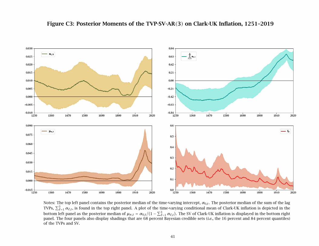
Figure C3: Posterior Moments of the TVP-SV-AR(3) on Clark-UK Inflation, 1251–2019

Notes: The top left panel contains the posterior median of the time-varying intercept, α0,t . The posterior median of the sum of the lag

TVPs,∑3ℓ=1αℓ,t , is found in the top right panel. A plot of the time-varying conditional mean of Clark-UK inflation is depicted in the

bottom left panel as the posterior median of µπ,t = α0,t

/(

1−∑3ℓ=1αℓ,t

)

. The SV of Clark-UK inflation is displayed in the bottom right

panel. The four panels also display shadings that are 68 percent Bayesian credible sets (i.e., the 16 percent and 84 percent quantiles)

of the TVPs and SV.

41

Figure C4: 1-Year Ahead Expected Clark-UK Inflation and Its Ex Post Forecast Error, 1251–2019

Notes: The top panel plots median 1-year ahead expected Clark-UK Inflation, Etπt+1. Expected inflation is estimated using the Kalman

filter, sample Clark-UK inflation, and the posterior distribution of the TVP-SV-AR(

3)

. The bottom panel contains the ex post forecast

error, πt+1 − Etπt+1. The panels also contain shadings that are 90 percent Bayesian credible sets (i.e., credible sets consisting of 5%

and 95% quantiles).

42

Figure C5: Predictability of Clark-UK Inflation 1-, 2-, 3-, and 5-Years Ahead, 1251–2019

Notes: The top left panel plots the median 1-year ahead R-square statistic, R21t , which is computed as described in equation

(

8)

, from

1251 to 2019. The shadings around R21t are 68% Bayesian uncertainty bands. Similarly, median R2

2t , R23t , and R2

5t appear in the top

right, bottom left, and bottom right panels along with 68% Bayesian uncertainty bands as the shadings. The R-square statistics are

computed using the posterior distribution of the TVP-SV-AR(

3)

.

43

Figure C6: Price-Level (In)Stability of Clark-UK Series, 1251–2019

Notes: The top left panel plots the median of the 1-year ahead square root of the sum of the conditional variance and the squared,

conditional mean,

√

vart(

pt+1 − Etpt+1

)

+

(

Etpt+1 − pt)2

, from 1251 to 2019. The shadings around this statistic are 90% Bayesian

uncertainty bands. The median 2-, 3-, and 5-year ahead price-level stability statistics are displayed in the top right, bottom left, and

bottom right panels along with shadings that are 90% Bayesian uncertainty bands. The price-level stability statistics are computed

using the posterior distribution of the TVP-SV-AR(

3)

.

44

Figure C7: UK Nominal and Real Short- and Long-Term Interest Rates

Notes: The top row plots UK nominal short- and long-term interest rates; see section 7 and the appendix for details. The bottom row

depicts ex ante short- and long-term real rates, rNS,i,t = RBofE,i,t − Etπt+1, in the left and right panels, where i = S(short) and L(long).

Short-term (long-term) rates begin in 1695 (1703) and end in 2019. One-year ahead expected inflation is computed using the posterior

distribution of the TVP-SV-AR(

3)

. In the bottom row of panels, the shadings are 90% Bayesian uncertainty bands.

45

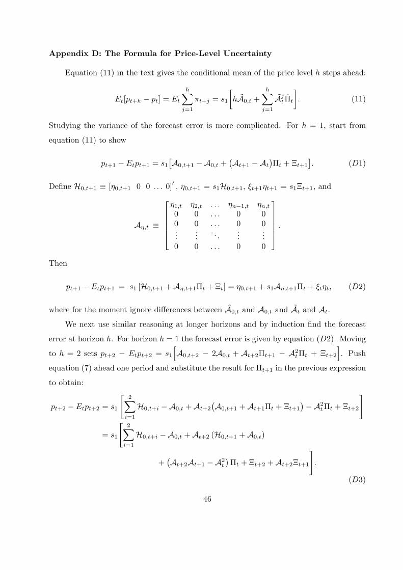
Appendix D: The Formula for Price-Level Uncertainty

Equation (11) in the text gives the conditional mean of the price level h steps ahead:

Et[pt+h − pt] = Et

h∑

j=1

πt+j = s1

[hA0,t +

h∑

j=1

Ajt Πt

]. (11)

Studying the variance of the forecast error is more complicated. For h = 1, start from

equation (11) to show

pt+1 − Etpt+1 = s1[A0,t+1 −A0,t +

(At+1 −At

)Πt + Ξt+1

]. (D1)

Define H0,t+1 ≡ [η0,t+1 0 0 . . . 0]′, η0,t+1 = s1H0,t+1, ξt+1ηt+1 = s1Ξt+1, and

Aη,t ≡

η1,t η2,t . . . ηn−1,t ηn,t0 0 . . . 0 00 0 . . . 0 0...

.... . .

......

0 0 . . . 0 0

.

Then

pt+1 − Etpt+1 = s1 [H0,t+1 +Aη,t+1Πt + Ξt] = η0,t+1 + s1Aη,t+1Πt + ξtηt, (D2)

where for the moment ignore differences between A0,t and A0,t and At and At.

We next use similar reasoning at longer horizons and by induction find the forecast

error at horizon h. For horizon h = 1 the forecast error is given by equation (D2). Moving

to h = 2 sets pt+2 − Etpt+2 = s1

[A0,t+2 − 2A0,t + At+2Πt+1 − A2

tΠt + Ξt+2

]. Push

equation (7) ahead one period and substitute the result for Πt+1 in the previous expression

to obtain:

pt+2 − Etpt+2 = s1

[2∑

i=1

H0,t+i −A0,t +At+2

(A0,t+1 +At+1Πt + Ξt+1

)−A2

tΠt + Ξt+2

]

= s1

[2∑

i=1

H0,t+i −A0,t +At+2 (H0,t+1 +A0,t)

+(At+2At+1 −A2

t

)Πt + Ξt+2 +At+2Ξt+1

].

(D3)

46

Using the same arguments at h = 3 gives

pt+3 − Etpt+3 = s1[A0,t+3 − 3A0,t +At+3Πt+2 −A3

tΠt + Ξt+3

]

= s1

[3∑

i=1

H0,t+i − 2A0,t +At+3

(A0,t+2 +At+2Πt+1 + Ξt+2

)

−A3tΠt + Ξt+3

]

= s1

[3∑

i=1

H0,t+i − 2A0,t +At+3

(2∑

i=1

H0,t+i +A0,t

)

+At+3At+2

(A0,t+1 +At+1Πt + Ξt+1

)−A3

tΠt

+ Ξt+3 +At+3Ξt+2

]

= s1

[3∑

i=1

H0,t+i − 2A0,t

+At+3

(2∑

i=1

H0,t+i +At+2H0,t+1

)+At+3At+2A0,t +At+3A0,t

+(At+3At+2At+1 −A3

t

)Πt + Ξt+3 +At+3Ξt+2 +At+3At+2Ξt+1

].

(D4)

By induction, the forecast error h-steps ahead is

pt+h − Etpt+h = s1

[H0,t,h +

h−1∑

j=1

h−1∏

ℓ=j

At+ℓ+1

H0,t,j

−

(h− 1

)−

h−1∑

j=1

h−1∏

ℓ=j

At+ℓ+1

A0,t

+

h∏

j=1

At+j −Aht

Πt + Ξt,h +

h−1∑

j=1

h−1∏

ℓ=j

At+ℓ+1

Ξt,j

], (D5)

where H0,t,j =[α0,t 0 0 . . . 0

]′, α0,t = α0,t +

∑ji=1 η0,t+i, Ξt,j =

[ξtǫt+j 0 0 . . . 0

]′,

and ξt= ξt

√exp(σφ

∏ji=1 φt+i

).

47

If the AUM is applied to the At+j that appear in equation (D5), the result is the local

approximation

pt+h − Etpt+h ≈ s1

[H0,t,h +

h−1∑

j=1

Aj+1t H0,t,j −

(h− 1

)−

h−1∑

j=1

Aj+1t

A0,t

+ Ξt+h +

h−1∑

j=1

Aj+1t Ξt+j

]

= s1

[h∑

j=1

H0,t+j +h−1∑

j=1

Aj+1t H0,t+j −

[(h− 1

)

−At

(Ip −Ah

t

)(Ip −At)

−1

]A0,t + Ξt,h +

h−1∑

j=1

Aj+1t Ξt,j

]. (D6)

The expression to the right of the (second) equality of equation (D6) shows the forecast

error of the conditional mean of accumulated h-year ahead inflation under the AUM as-

sumption depends on innovations, η0,t, to the time-varying intercept of the AR(n), α0,t, SV

in Ξt, but is net of the difference between hα0,t and µπ,t = s1 (Ip −At)−1 A0,t reduced by

At

(In −Ah

t

). Also, as h → ∞, s1At

(In −Ah

t

)(In −At)

−1 A0,t → s1At (In −At)−1 A0,t

= µπ,t

∑nℓ=1 αℓ,t < ∞. Hence,

(h− 1

)A0,t acts as a counterweight to the accumulation of

SV as the forecast horizon increases in equation (D6).

Cogley and Sargent (2016) and Cogley, Sargent, and Surico (2015) assess the volatil-

ity or uncertainty surrounding Et[pt+h − pt]. Their notion of price-level uncertainty is

vart (pt+h − pt), which is equation (8) of the latter paper. Since the conditional variance

telescopes the price level between dates t+h−1 and t+1, the variance of equation (D6) is:

vart(pt+h − Etpt+h

)≈ s1Et

H0,t,j +

h−1∑

j=1

Aj+1t H0,t,j

H0,t,j +

h−1∑

j=1

Aj+1t H0,t,j

′

s′1

+ s1Et

Ξt,h +

h−1∑

j=1

Aj+1t Ξt,j

Ξt,h +

h−1∑

j=1

Aj+1t Ξt,j

′

s′1

48

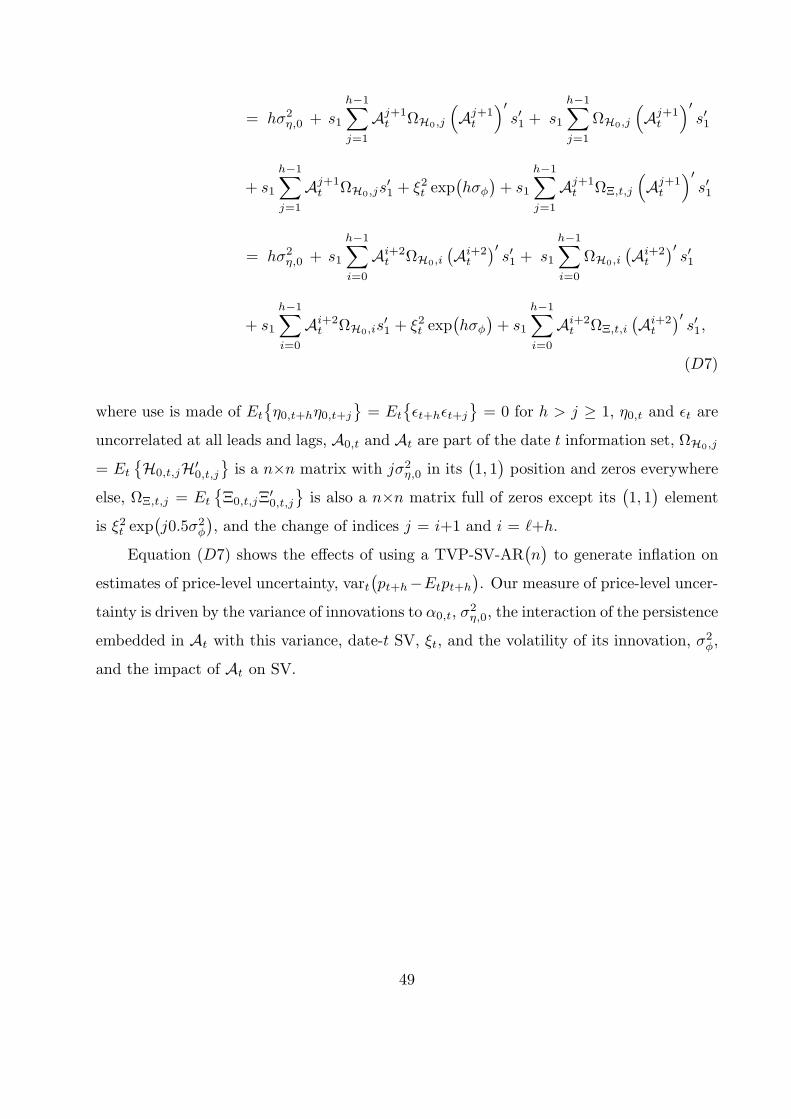
= hσ2η,0 + s1

h−1∑

j=1

Aj+1t ΩH0,j

(Aj+1

t

)′s′1 + s1

h−1∑

j=1

ΩH0,j

(Aj+1

t

)′s′1

+ s1

h−1∑

j=1

Aj+1t ΩH0,js

′1 + ξ2t exp

(hσφ

)+ s1

h−1∑

j=1

Aj+1t ΩΞ,t,j

(Aj+1

t

)′s′1

= hσ2η,0 + s1

h−1∑

i=0

Ai+2t ΩH0,i

(Ai+2

t

)′s′1 + s1

h−1∑

i=0

ΩH0,i

(Ai+2

t

)′s′1

+ s1

h−1∑

i=0

Ai+2t ΩH0,is

′1 + ξ2t exp

(hσφ

)+ s1

h−1∑

i=0

Ai+2t ΩΞ,t,i

(Ai+2

t

)′s′1,

(D7)

where use is made of Et

η0,t+hη0,t+j

= Et

ǫt+hǫt+j

= 0 for h > j ≥ 1, η0,t and ǫt are

uncorrelated at all leads and lags, A0,t and At are part of the date t information set, ΩH0,j

= Et

H0,t,jH

′0,t,j

is a n×n matrix with jσ2

η,0 in its(1, 1)position and zeros everywhere

else, ΩΞ,t,j = Et

Ξ0,t,jΞ

′0,t,j

is also a n×n matrix full of zeros except its

(1, 1)element

is ξ2t exp(j0.5σ2

φ

), and the change of indices j = i+1 and i = ℓ+h.

Equation (D7) shows the effects of using a TVP-SV-AR(n)to generate inflation on

estimates of price-level uncertainty, vart(pt+h−Etpt+h

). Our measure of price-level uncer-

tainty is driven by the variance of innovations to α0,t, σ2η,0, the interaction of the persistence

embedded in At with this variance, date-t SV, ξt, and the volatility of its innovation, σ2φ,

and the impact of At on SV.

49