Production Planning & Scheduling in Large Corporations.

Production Planning & Scheduling in Large Corporations

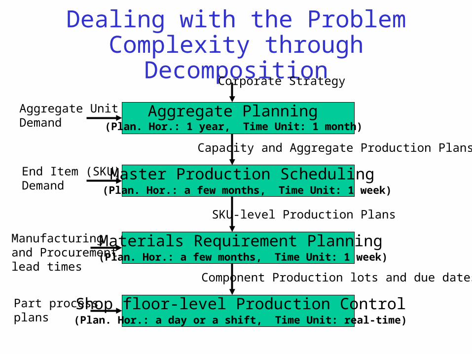
Dealing with the Problem Complexity through Decomposition

Aggregate Planning

Master Production Scheduling

Materials Requirement Planning

Aggregate UnitDemand

End Item (SKU)Demand

Corporate Strategy

Capacity and Aggregate Production Plans

SKU-level Production Plans

Manufacturingand Procurementlead times

Component Production lots and due dates

Part processplans

(Plan. Hor.: 1 year, Time Unit: 1 month)

(Plan. Hor.: a few months, Time Unit: 1 week)

(Plan. Hor.: a few months, Time Unit: 1 week)

Shop floor-level Production Control(Plan. Hor.: a day or a shift, Time Unit: real-time)

Aggregate Planning

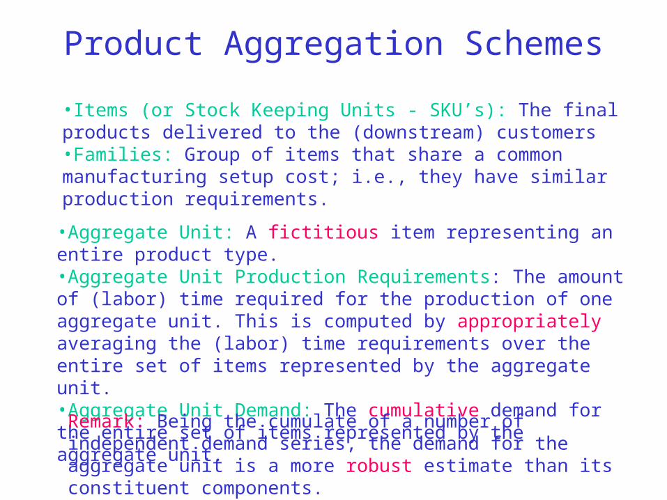
Product Aggregation Schemes

•Items (or Stock Keeping Units - SKU’s): The final products delivered to the (downstream) customers•Families: Group of items that share a common manufacturing setup cost; i.e., they have similar production requirements.

•Aggregate Unit: A fictitious item representing an entire product type.•Aggregate Unit Production Requirements: The amount of (labor) time required for the production of one aggregate unit. This is computed by appropriately averaging the (labor) time requirements over the entire set of items represented by the aggregate unit.•Aggregate Unit Demand: The cumulative demand for the entire set of items represented by the aggregate unit.

Remark: Being the cumulate of a number of independent demand series, the demand for the aggregate unit is a more robust estimate than its constituent components.

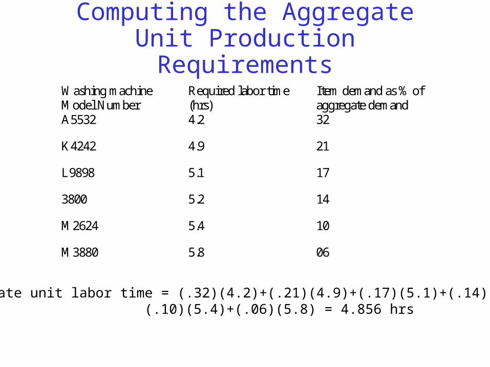
Computing the Aggregate Unit Production Requirements

Washing machineModel Number

Required labor time(hrs)

Item demand as % ofaggregate demand

A5532 4.2 32

K4242 4.9 21

L9898 5.1 17

3800 5.2 14

M2624 5.4 10

M3880 5.8 06

Aggregate unit labor time = (.32)(4.2)+(.21)(4.9)+(.17)(5.1)+(.14)(5.2)+(.10)(5.4)+(.06)(5.8) = 4.856 hrs

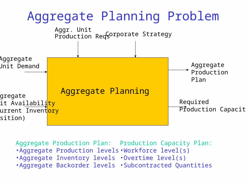
Aggregate Planning Problem

Aggregate Planning

AggregateUnit Demand

AggregateUnit Availability(Current InventoryPosition)

Aggregate Production Plan

Required Production Capacity

Aggr. UnitProduction Reqs Corporate Strategy

Aggregate Production Plan:•Aggregate Production levels•Aggregate Inventory levels•Aggregate Backorder levels

Production Capacity Plan:•Workforce level(s)•Overtime level(s)•Subcontracted Quantities

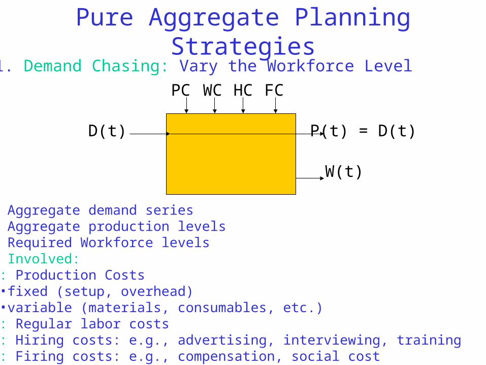
Pure Aggregate Planning Strategies1. Demand Chasing: Vary the Workforce Level

D(t) P(t) = D(t)

W(t)

PC WC HC FC

•D(t): Aggregate demand series•P(t): Aggregate production levels•W(t): Required Workforce levels•Costs Involved:

•PC: Production Costs•fixed (setup, overhead)•variable (materials, consumables, etc.)

•WC: Regular labor costs•HC: Hiring costs: e.g., advertising, interviewing, training•FC: Firing costs: e.g., compensation, social cost

Pure Aggregate Planning Strategies2. Varying Production Capacity with Constant Workforce:

D(t) P(t)

O(t)

PC WC OC UC

U(t)

S(t)

SC

W = constant•S(t): Subcontracted quantities•O(t): Overtime levels•U(t): Undertime levels•Costs involved:

•PC, WC: as before•SC: subcontracting costs: e.g., purchasing, transport, quality, etc.•OC: overtime costs: incremental cost of producing one unit in overtime•(UC: undertime costs: this is hidden in WC)

Pure Aggregate Planning Strategies

3. Accumulating (Seasonal) Inventories:

D(t) P(t)

I(t)

PC WC IC

W(t), O(t), U(t), S(t) = constant

•I(t): Accumulated Inventory levels•Costs involved:

•PC, WC: as before•IC: inventory holding costs: e.g., interest lost, storage space, pilferage, obsolescence, etc.

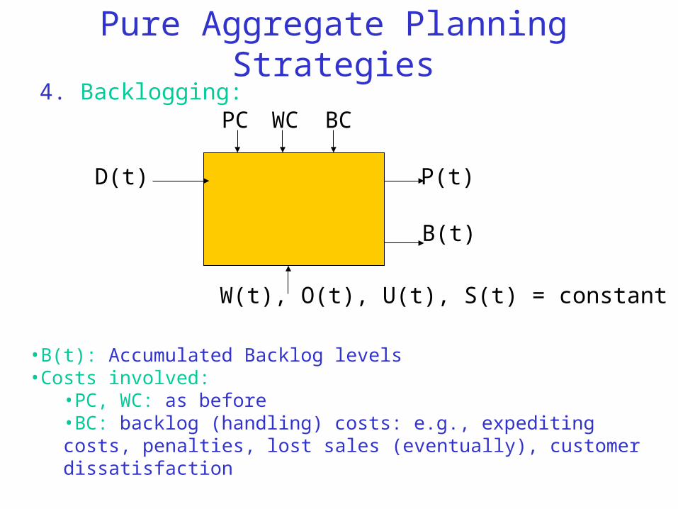
Pure Aggregate Planning Strategies4. Backlogging:

D(t) P(t)

B(t)

PC WC BC

W(t), O(t), U(t), S(t) = constant

•B(t): Accumulated Backlog levels•Costs involved:

•PC, WC: as before•BC: backlog (handling) costs: e.g., expediting costs, penalties, lost sales (eventually), customer dissatisfaction

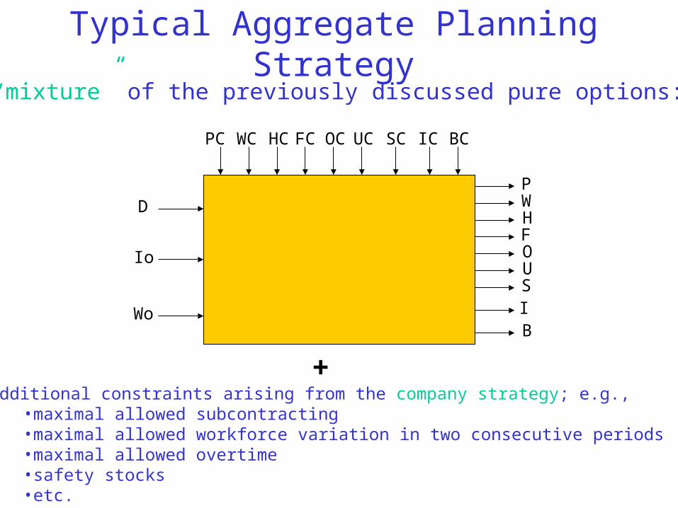
Typical Aggregate Planning StrategyA “mixture” of the previously discussed pure options:

D

PC WC HC FC OC UC SC IC BC

PWHFOUSIB

+Additional constraints arising from the company strategy; e.g.,

•maximal allowed subcontracting•maximal allowed workforce variation in two consecutive periods•maximal allowed overtime•safety stocks•etc.

Io

Wo

Solution Approaches

• Graphical Approaches: Spreadsheet-based simulation

• Analytical Approaches: Mathematical (mainly linear programming) Programming formulations

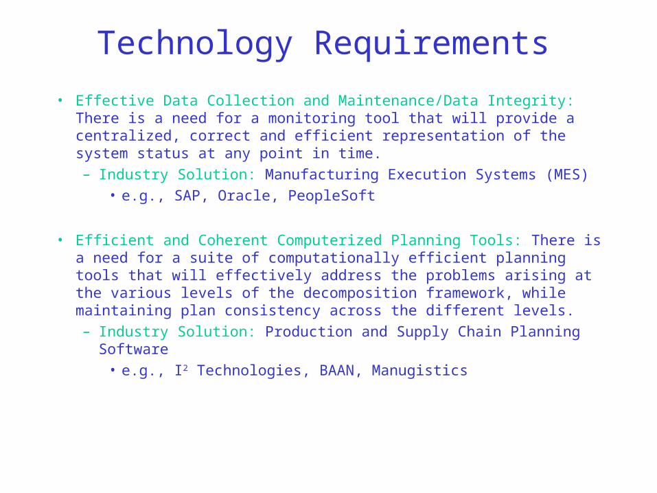
Technology Requirements

• Effective Data Collection and Maintenance/Data Integrity: There is a need for a monitoring tool that will provide a centralized, correct and efficient representation of the system status at any point in time.

– Industry Solution: Manufacturing Execution Systems (MES)

• e.g., SAP, Oracle, PeopleSoft

• Efficient and Coherent Computerized Planning Tools: There is a need for a suite of computationally efficient planning tools that will effectively address the problems arising at the various levels of the decomposition framework, while maintaining plan consistency across the different levels.

– Industry Solution: Production and Supply Chain Planning Software

• e.g., I2 Technologies, BAAN, Manugistics

Aggregate Planning:Example

(Adapted from Chase and Aquilano,

“Fundamentals of Operations Management”, Irwin Pub., 1991)

Example: IntroductionA vacuum cleaner manufacturer tries to “plan ahead” in order to effectively address the seasonal variation appearing in the annualdemand of its products. A planning horizon of 6 months is used.The (aggregate) demand forecast for the next six months along the number of working days are as follows:

Month Demand Forecast No. of Working DaysJan. 1,800 22Febr. 1,500 19March 1,100 21April 900 21May 1,100 22June 1,600 20

Total: 8,000 units Total: 125 Days

Example: Introduction (cont.)The associated cost break-down is as follows:

Cost Item Cost($)Material $100 per unitInventory Holding $5 per unit per monthMarginal Stockout $10 per unit per monthMarginal Cost of Subcontracting $20 per unit(Cost of buying less material costs)Hiring and Training $1000 per workerLayoff $1500 per workerRegular Labor cost per hour $15 per employee per hourOvertime labor cost per hour $20 per employee per hour

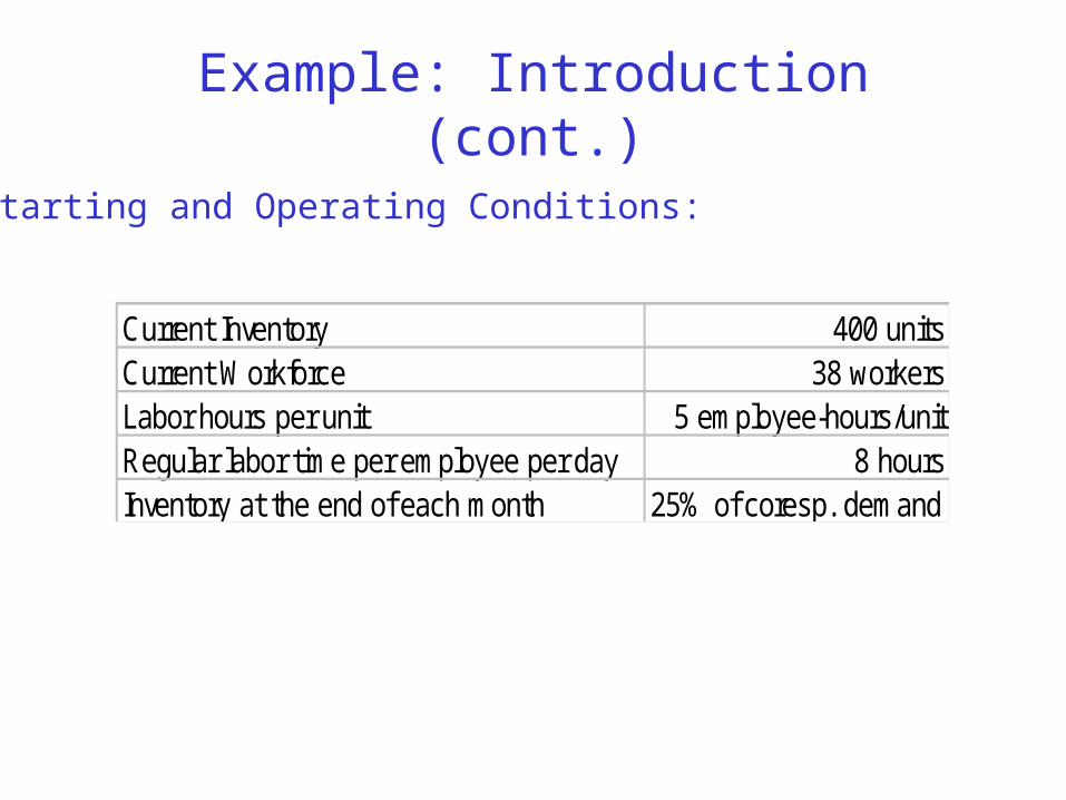
Example: Introduction (cont.)

Starting and Operating Conditions:

Current Inventory 400 unitsCurrent Workforce 38 workersLabor hours per unit 5 employee-hours/unitRegular labor time per employee per day 8 hoursInventory at the end of each month 25% of coresp. demand

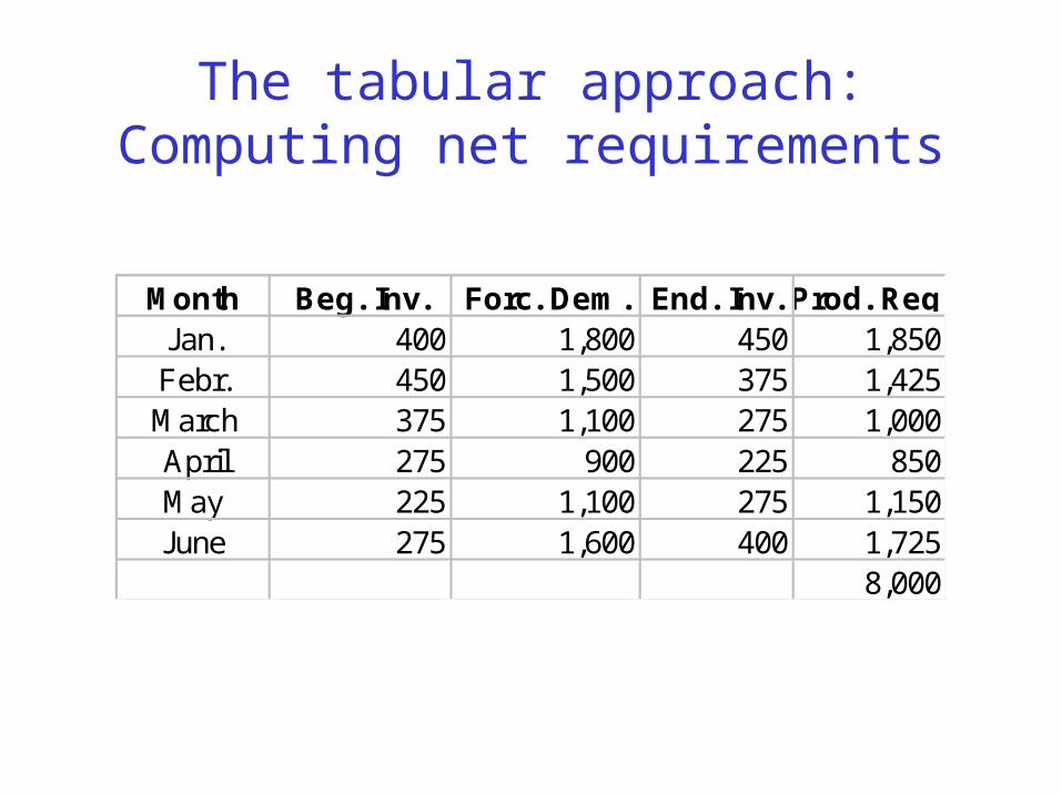
The tabular approach:Computing net requirements

Month Beg. Inv. Forc. Dem. End. Inv. Prod. Req.Jan. 400 1,800 450 1,850Febr. 450 1,500 375 1,425March 375 1,100 275 1,000April 275 900 225 850May 225 1,100 275 1,150June 275 1,600 400 1,725

8,000

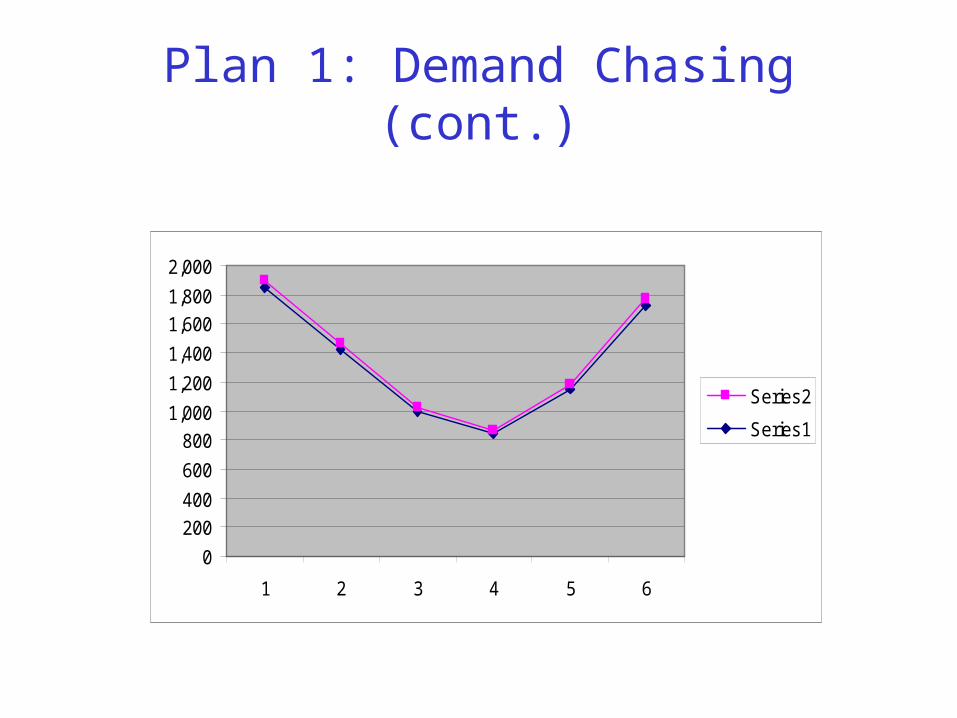
Plan 1: Demand Chasing

Produce exactly the quantities required for each period throughregular labor, by varying the workforce size.

Month Prod. Req. Req. Labor Hours Work Days Workers PC WC HC FCJan. 1,850 9,250 22 53 185000 139920 15000 0Febr. 1,425 7,125 19 47 142500 107160 0 9000March 1,000 5,000 21 30 100000 75600 0 25500April 850 4,250 21 25 85000 63000 0 7500May 1,150 5,750 22 33 115000 87120 8000 0June 1,725 8,625 20 54 172500 129600 21000 0

800000 602400 44000 42000TC= 1488400

Plan 1: Demand Chasing (cont.)

0

200

400

600

800

1,000

1,200

1,400

1,600

1,800

2,000

1 2 3 4 5 6

Series2

Series1

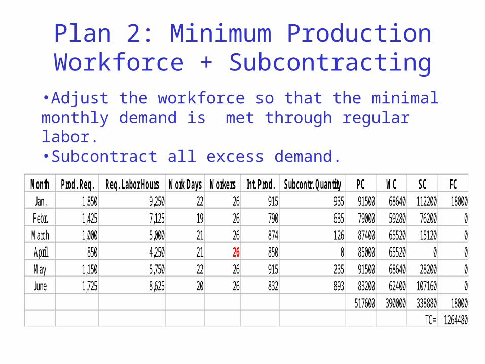
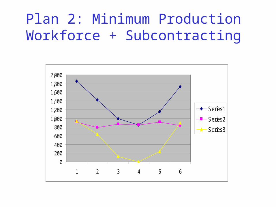
Plan 2: Minimum Production Workforce + Subcontracting

•Adjust the workforce so that the minimal monthly demand is met through regular labor.•Subcontract all excess demand.

Month Prod. Req. Req. Labor Hours Work Days Workers Int. Prod. Subcontr. Quantity PC WC SC FCJan. 1,850 9,250 22 26 915 935 91500 68640 112200 18000Febr. 1,425 7,125 19 26 790 635 79000 59280 76200 0March 1,000 5,000 21 26 874 126 87400 65520 15120 0April 850 4,250 21 26 850 0 85000 65520 0 0May 1,150 5,750 22 26 915 235 91500 68640 28200 0June 1,725 8,625 20 26 832 893 83200 62400 107160 0

517600 390000 338880 18000TC= 1264480

Plan 2: Minimum Production Workforce + Subcontracting

0

200

400

600

800

1,000

1,200

1,400

1,600

1,800

2,000

1 2 3 4 5 6

Series1

Series2

Series3

Plan 3: Anticipatory (Seasonal)

Inventories + Backlogging •Employ the minimal workforce level that can cover the total production requirements over the considered planning horizon, by working only regular hours.•Take care of the demand fluctuations by building anticipatory inventories and/or backlogging excess demand.

Month Prod. Req. Work Days Workers Act. Prod. Inventory Backlogs PC WC IC BCJan. 1,800 22 38 1338 0 62 133800 100320 0 620Febr. 1,500 19 38 1155 0 407 115500 86640 0 4070March 1,100 21 38 1277 0 230 127700 95760 0 2300April 900 21 38 1277 147 0 127700 95760 735 0May 1,100 22 38 1338 385 0 133800 100320 1925 0June 1,600 20 38 1215 0 0 121500 91200 0 0

8000 125 7600 760000 570000 2660 6990TC= 1339650

Plan 3: Anticipatory (Seasonal) Inventories + Backlogging (cont.)

-1,000

-500

0

500

1,000

1,500

2,000

1 2 3 4 5 6

Series1

Series2

Series3

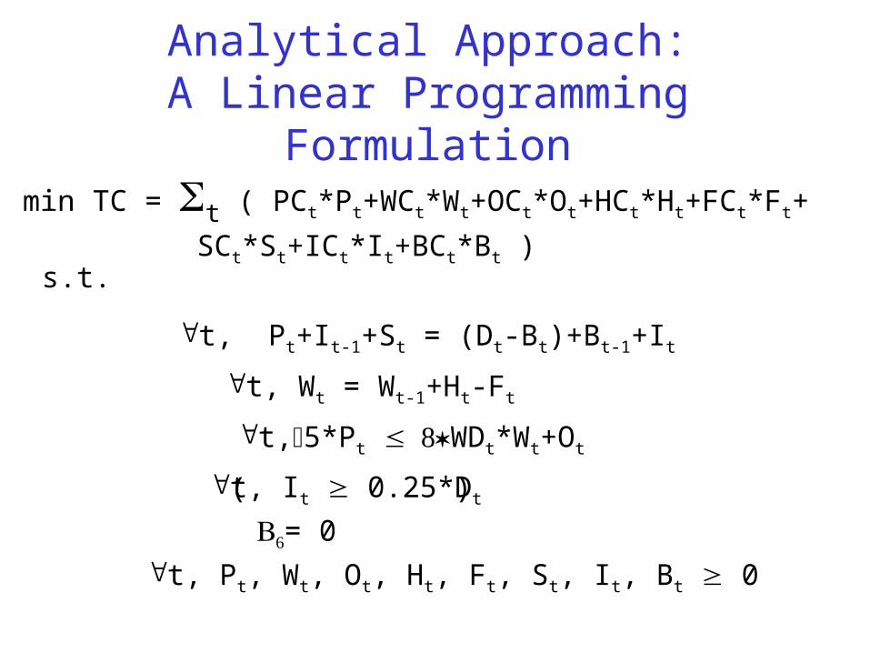
Analytical Approach:A Linear Programming Formulation

min TC = t ( PCt*Pt+WCt*Wt+OCt*Ot+HCt*Ht+FCt*Ft+

SCt*St+ICt*It+BCt*Bt )s.t.

t, Pt+It-1+St = (Dt-Bt)+Bt-1+It

t, Wt = Wt-1+Ht-Ft

t,5*Pt WDt*Wt+Ot

t, It 0.25*Dt

= 0

t, Pt, Wt, Ot, Ht, Ft, St, It, Bt 0

( )

Proactive approaches to demand management

• Influencing demand variation so that it aligns to available production capacity:– advertising

– promotional plans

– pricing

(e.g., airline and hotel weekend discounts, telecommunication companies’ weekend rates)

• “Counter-seasonal” product (and service) mixing: Develop a product mix with antithetic (seasonal) trends that level the cumulative required production capacity.– (e.g., lawn mowers and snow blowers)

Disaggregation and Master Production Scheduling

(MPS)

The (Master) Production Scheduling Problem

MPS

Placed Orders

Forecasted DemandCurrent and PlannedAvailability, eg.,•Initial Inventory,•Initiated Production,•Subcontracted quantities

Master ProductionSchedule:When & How Muchto produce for eachproduct

CapacityConsts.

CompanyPolicies

EconomicConsiderations

ProductCharact.

PlanningHorizon

Timeunit

CapacityPlanning

(Typical) Analytical Approaches to MPS

• Recognizing that switching production from item to item (or family to family) requires significant set-up times, during which the effective productivity of the line is equal to zero, these (formal) approaches try to apportion the planned production capacity to the various items in a way that meets their effective demand while it minimizes the (long-run) number of set-ups.

• However, they tend to be technically cumbersome and/or limiting in terms of modeling capability, and therefore, not extensively used in practice.

• Example:– Textbook, Section 5.7.1

The Driving Logic behind the Empirical Approach

Demand Availability:•Initial Inventory Position•Scheduled Receipts due to initiated production or subcontracting

Future inventories

NetRequirements

Lot Sizing

ScheduledReleases

Resource (Fermentor)Occupancy Product i

FeasibilityTesting

Master Production Schedule

ScheduleInfeasibilities

ReviseProd. Reqs

Compute FutureInventory Positions

McGuinnes & Co. MicrobreweryCase Study

Company Description

• One of the three largest microbreweries in Atlanta area

• Company started in 1995

• A 12,000sq. ft. production facility and warehouse in the Chattahoochee Industrial Park

• The company is run by its owner, Mr. McGuinness

• Three full-time and two-part time employees, and occasionally hires part-time help

• Last year’s sales: > 35,000 cases => > $180,000

• Average weekly sales: 500-800 cases

Company Products

• Pale Ale: The oldest company product. Since May 2000, this product is also offered in the NY and Boston areas, through a major national distributor.

• Product monthly sales over the last four years (1997-2000) in cases of beer:

Sales

0

200

400

600

800

1000

1200

1400

1600

1 4 7 10 13 16 19 22 25 28 31 34 37 40 43 46

Sales

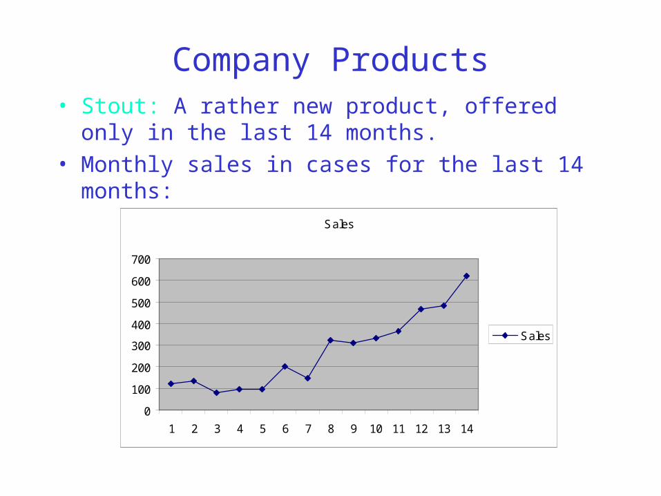
Company Products• Stout: A rather new product, offered only in the last 14

months.

• Monthly sales in cases for the last 14 months:

Sales

0

100

200

300

400

500

600

700

1 2 3 4 5 6 7 8 9 10 11 12 13 14

Sales

Company Products

• Winter Ale: A seasonal beer, offered primarily during the winter period (from October to April).

• Product monthly sales over the last 4 years:

Sales

0

200

400

600

800

1000

1200

1400

1 4 7 10 13 16 19 22 25 28 31 34 37 40 43 46

Sales

Company Products

• Summer Brew: A seasonal beer offered primarily during the summer season. A new product offered over the last two years.

• Product monthly sales in cases over the last two years:

Sales

0

100

200

300

400

500

600

700

1 3 5 7 9 11 13 15 17 19 21 23

Sales

Company Products

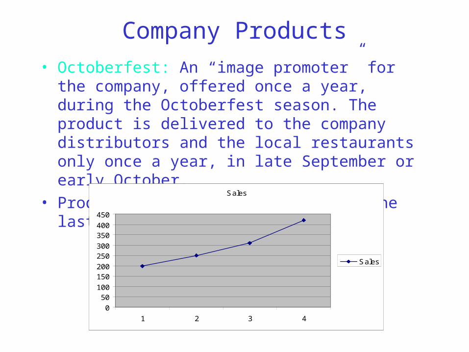
• Octoberfest: An “image promoter” for the company, offered once a year, during the Octoberfest season. The product is delivered to the company distributors and the local restaurants only once a year, in late September or early October.

• Product annual sales in cases for the last four years:

Sales

0

50100

150200

250300

350400

450

1 2 3 4

Sales

Company Operations

Mashing(1 mashing tun)

Boiling(1 brew kettle)

Fermentation(3 40-barrelferm. tanks)

Filtering(1 filter tank)

Bottling(1 bottling

station)

Grain cracking(1 millingmachine)

Fermentation Times:Brew Ferm. Time

Pale Ale 2 weeks

Stout 3 weeks

Winter Ale 2 weeks

Summer Brew 2 weeks

Octoberfest 8-10 weeks

Company Challenges

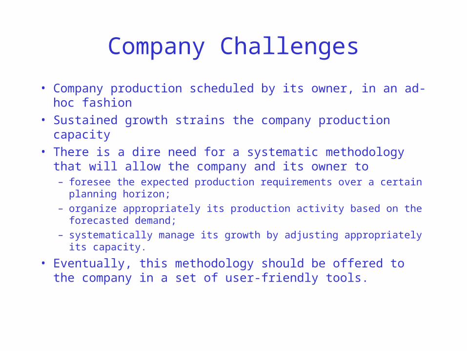
• Company production scheduled by its owner, in an ad-hoc fashion

• Sustained growth strains the company production capacity• There is a dire need for a systematic methodology that will

allow the company and its owner to– foresee the expected production requirements over a certain planning

horizon;

– organize appropriately its production activity based on the forecasted demand;

– systematically manage its growth by adjusting appropriately its capacity.

• Eventually, this methodology should be offered to the company in a set of user-friendly tools.

Example: Implementing the Empirical Approach in Excel

# Fermentors: 1 Unit Cap: 200 Shelf Life: 20

Microbrewery PerformanceWeek 0 1 2 3 4 5 6 7 8 9 10# Fermentors Req'd 0 0 0 0 0 0 0 0 0 0Feasible Loading?Min # Fermentors Req'd 2 2 2 2 2 2 2 2 2 2Fermentor Utilization 0% 0% 0% 0% 0% 0% 0% 0% 0% 0%Total Spoilage 0 0 0 0 0 0 0 0 0 0

Pale Ale Fermentation Time: 2Week 0 1 2 3 4 5 6 7 8 9 10Demand 45 50 40 40 40 40 40 40 40 40Scheduled Receipts 200Fermentors Released 1Inventory SpoilageInventory Position 100 255 205 165 125 85 45 5 -35 -40 -40Net Requirements 35 40 40Batched Net ReceiptsScheduled ReleasesFermentors SeizedTotal Fermentors Occupied

Stout Fermentation Time: 3Week 0 1 2 3 4 5 6 7 8 9 10Demand 35 40 30 30 40 40 40 40 50 50Scheduled ReceiptsFermentors ReleasedInventory SpoilageInventory Position 150 115 75 45 15 -25 -40 -40 -40 -50 -50Net Requirements 25 40 40 40 50 50Batched Net ReceiptsScheduled ReleasesFermentors SeizedTotal Fermentors Occupied

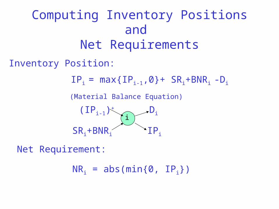
Computing Inventory Positions and Net Requirements

Net Requirement:

NRi = abs(min{0, IPi})

Inventory Position:

IPi = max{IPi-1,0}+ SRi+BNRi -Di

(Material Balance Equation)

iDi

IPi

(IPi-1)+

SRi+BNRi

Problem Decision Variables: Scheduled Releases



Pale Ale Fermentation Time: 2Week 0 1 2 3 4 5 6 7 8 9 10Demand 45 50 40 40 40 40 40 40 40 40Scheduled Receipts 200Fermentors Released 1Inventory SpoilageInventory Position 100 255 205 165 125 85 45 5 165 125 85Net RequirementsBatched Net Receipts 200Scheduled Releases 200Fermentors Seized 1Total Fermentors Occupied 1 1


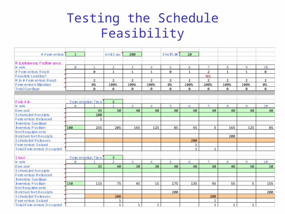
Testing the Schedule Feasibility


Microbrewery PerformanceWeek 0 1 2 3 4 5 6 7 8 9 10# Fermentors Req'd 0 1 1 1 0 1 2 1 1 0Feasible Loading? NOMin # Fermentors Req'd 2 2 2 2 2 2 2 2 2 2Fermentor Utilization 0% 100% 100% 100% 0% 100% 200% 100% 100% 0%Total Spoilage 0 0 0 0 0 0 0 0 0 0


Stout Fermentation Time: 3Week 0 1 2 3 4 5 6 7 8 9 10Demand 35 40 30 30 40 40 40 40 50 50Scheduled ReceiptsFermentors ReleasedInventory SpoilageInventory Position 150 115 75 45 15 175 135 95 55 5 155Net RequirementsBatched Net Receipts 200 200Scheduled Releases 200 200Fermentors Seized 1 1Total Fermentors Occupied 1 1 1 1 1 1

Fixing the Original Schedule




Stout Fermentation Time: 3Week 0 1 2 3 4 5 6 7 8 9 10Demand 35 40 30 30 40 40 40 40 50 50Scheduled ReceiptsFermentors ReleasedInventory SpoilageInventory Position 150 115 75 45 15 175 135 95 55 5 155Net RequirementsBatched Net Receipts 200 200Scheduled Releases 200 200Fermentors Seized 1 1Total Fermentors Occupied 1 1 1 1 1 1

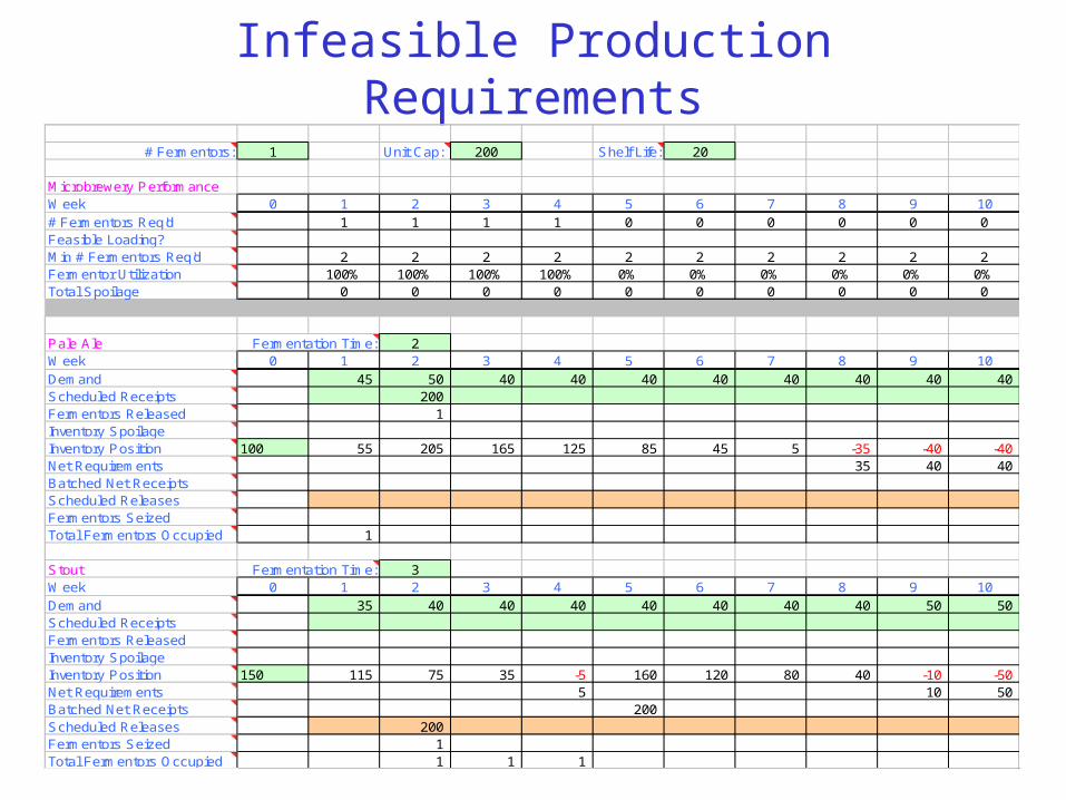
Infeasible Production Requirements



Pale Ale Fermentation Time: 2Week 0 1 2 3 4 5 6 7 8 9 10Demand 45 50 40 40 40 40 40 40 40 40Scheduled Receipts 200Fermentors Released 1Inventory SpoilageInventory Position 100 55 205 165 125 85 45 5 -35 -40 -40Net Requirements 35 40 40Batched Net ReceiptsScheduled ReleasesFermentors SeizedTotal Fermentors Occupied 1

Stout Fermentation Time: 3Week 0 1 2 3 4 5 6 7 8 9 10Demand 35 40 40 40 40 40 40 40 50 50Scheduled ReceiptsFermentors ReleasedInventory SpoilageInventory Position 150 115 75 35 -5 160 120 80 40 -10 -50Net Requirements 5 10 50Batched Net Receipts 200Scheduled Releases 200Fermentors Seized 1Total Fermentors Occupied 1 1 1

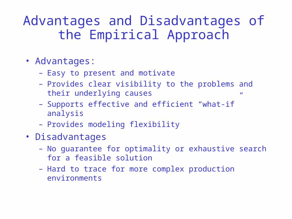
Advantages and Disadvantages of the Empirical Approach

• Advantages:– Easy to present and motivate

– Provides clear visibility to the problems and their underlying causes

– Supports effective and efficient “what-if” analysis

– Provides modeling flexibility

• Disadvantages– No guarantee for optimality or exhaustive search for a feasible

solution

– Hard to trace for more complex production environments

Modeling the Inventory Spoilage



Pale Ale Fermentation Time: 2Week 0 1 2 3 4 5 6 7 8 9 10Demand 45 50 40 40 40 40 40 40 40 40Scheduled Receipts 200Fermentors Released 1Inventory Spoilage 45Inventory Position 100 255 205 165 125 85 45 -40 -40 -40 -40Net Requirements 40 40 40 40Batched Net ReceiptsScheduled ReleasesFermentors SeizedTotal Fermentors Occupied


A feasible schedule with spoilage effects



Pale Ale Fermentation Time: 2Week 0 1 2 3 4 5 6 7 8 9 10Demand 45 50 40 40 40 40 40 40 40 40Scheduled Receipts 200Fermentors Released 1Inventory Spoilage 45Inventory Position 100 255 205 165 125 85 245 160 120 80 40Net RequirementsBatched Net Receipts 200Scheduled Releases 200Fermentors Seized 1Total Fermentors Occupied 1 1

Stout Fermentation Time: 3Week 0 1 2 3 4 5 6 7 8 9 10Demand 35 40 30 30 40 40 40 40 50 50Scheduled ReceiptsFermentors ReleasedInventory Spoilage 5Inventory Position 150 115 75 45 215 175 135 95 55 5 150Net RequirementsBatched Net Receipts 200 200Scheduled Releases 200 200Fermentors Seized 1 1Total Fermentors Occupied 1 1 1 1 1 1

Computing Spoilage and Modified Inventory Position

Spoilage:

SPi = max{0, IPi-1-SRi-1+SRi-2+…+SRi-sl+1) -BNRi-1+BNRi-2+…+BNRi-sl+1)}

Inventory Position:

IPi = max{IPi-1,0}+ SRi+BNRi -Di-SPi

(Material Balance Equation)

iDi

IPi

(IPi-1)+

SRi+BNRi

SPi

Materials Requirements Planning(MRP)

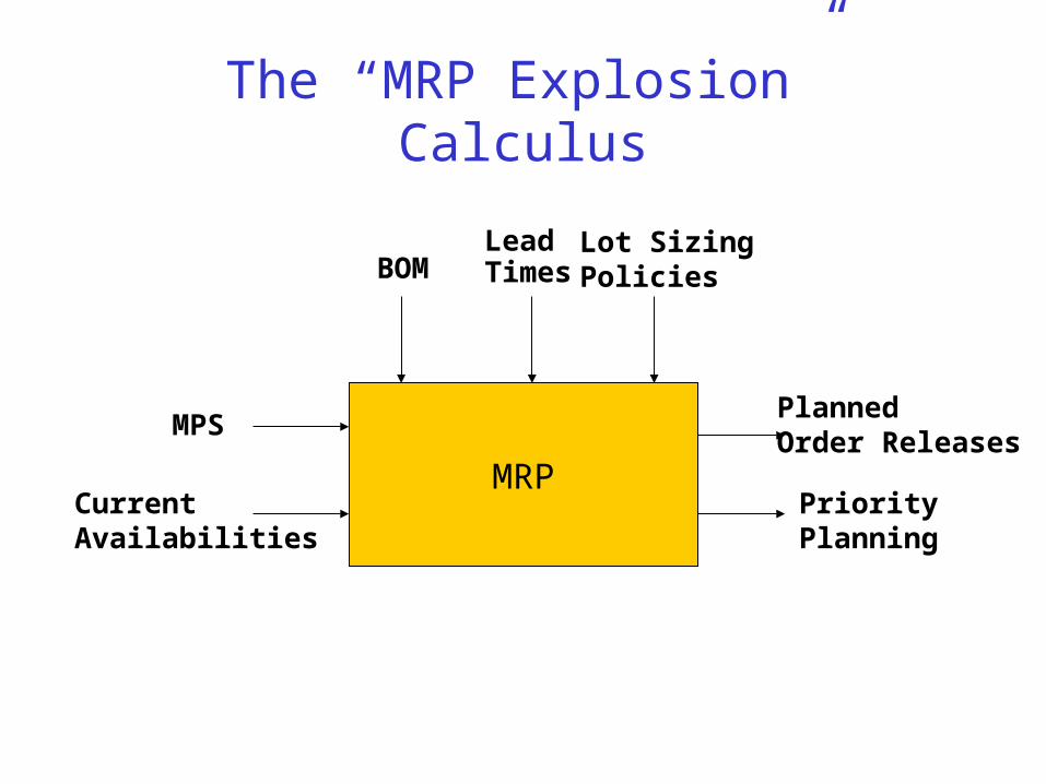
The “MRP Explosion” Calculus

BOM

MRP

MPS

Current Availabilities

PlannedOrder Releases

PriorityPlanning

LeadTimes

Lot SizingPolicies

Example: The (complete) MRP Explosion Calculus

(J. Heizer and B. Render “Operations Management”, 6th Ed. Prentice Hall)

Item BOM:

Alpha

C(2)D(2)

B(1) C(1)

E(1)

E(1)

F(1)

F(1)

Item Lead Time Current Inv. Pos.Alpha 1 10

B 2 20C 3 0D 1 100E 1 10F 1 50

Gross Reqs for AlphaPeriod 6 7 8 9 10 11 12 13Gross Reqs. 50 50 100

Item Levels:

Level 0: Alpha Level 1: B Level 2: C, D Level 3: E, F

The “MRP Explosion” Calculus

Level 0

Level 1

Level 2

Level N

InitialInventories

ScheduledReceipts

External Demand

CapacityPlanning

Planned Order ReleasesGross Requirements

Capacity Planning (Example)

Availablelaborhours

Periods1 2 3 4 5 6 7 8

50

100

150

Computing the item Scheduled Releases

Item CPeriod 1 2 3 4 5 6 7 8 9 10 11 12Gross Requirements 12 10 90 75Scheduled Receipts 20Inventory Position: 20 20 40 40 40 40 28 18 18 -72 0 -75 0Net Requirements 72 75Planned Sched. Receipts 72 75Planned Sched. Releases 72 75

Synthesizingitem demand

series

ProjectingInv. Positions

andNet Reqs.

Lot SizingTime-

Phasing

ParentSched. Rel.

Item ExternalDemand

Gross Reqs

ScheduledReceipts

InitialInventory

Safety StockRequirements

NetReqs

Lot SizingPolicy

Planned OrderReceipts

Lead Time

Planned OrderReleases

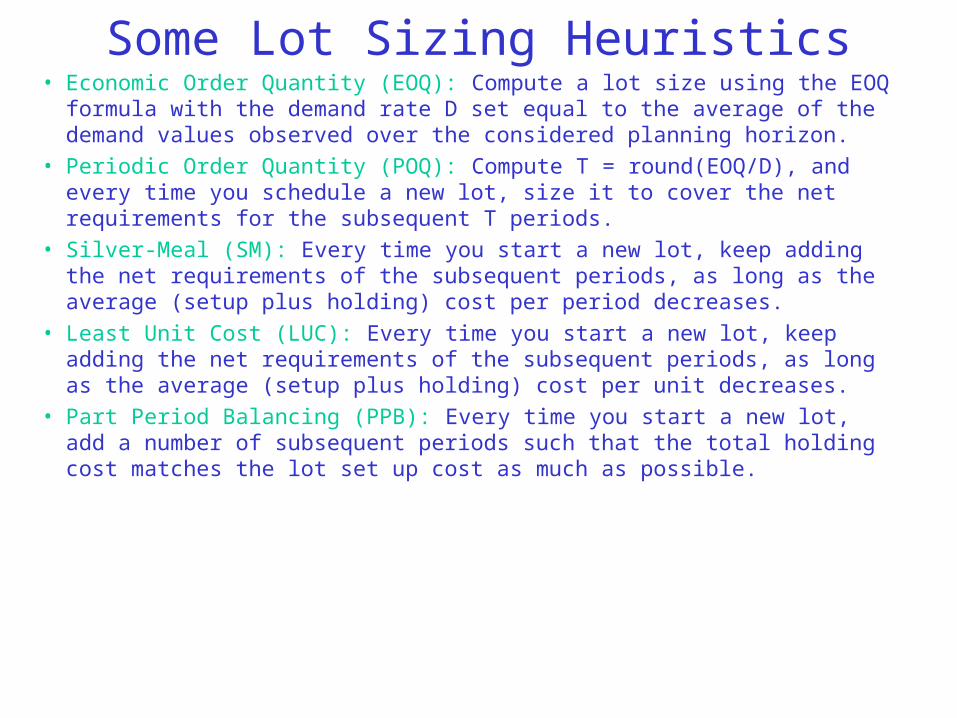
Some Lot Sizing Heuristics• Economic Order Quantity (EOQ): Compute a lot size using the EOQ formula with the

demand rate D set equal to the average of the demand values observed over the considered planning horizon.

• Periodic Order Quantity (POQ): Compute T = round(EOQ/D), and every time you schedule a new lot, size it to cover the net requirements for the subsequent T periods.

• Silver-Meal (SM): Every time you start a new lot, keep adding the net requirements of the subsequent periods, as long as the average (setup plus holding) cost per period decreases.

• Least Unit Cost (LUC): Every time you start a new lot, keep adding the net requirements of the subsequent periods, as long as the average (setup plus holding) cost per unit decreases.

• Part Period Balancing (PPB): Every time you start a new lot, add a number of subsequent periods such that the total holding cost matches the lot set up cost as much as possible.

Shop floor-level Production Control / Scheduling

General Problem Definition

Determine the timing of

– the releases of the various production lots on the shop-floor and

– the allocation to them of the system resources required for the execution of their various operations

so that the production plans decided at the tactical planning - i.e., MPS & MRP - level are observed as close as possible.

A modeling absrtaction

• M: number of machine types / workstations.• N: number of jobs to be scheduled.• Job routing: an ordered list / sequence of machines that a job

needs to visit in order to be completed.• Operation: a single processing step executed during the job visit

to a machine.• P_j: the set of operations in the routing of job j.• t_kj: the processing time for the k-th operation of job j.• d_j: due date for job j.• r_j: the release date of job j, i.e., the date at which the material

required for starting the job processing will be available.

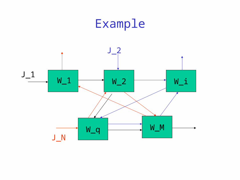
Example

W_q

W_2 W_i

W_M

W_1J_1

J_2

J_N

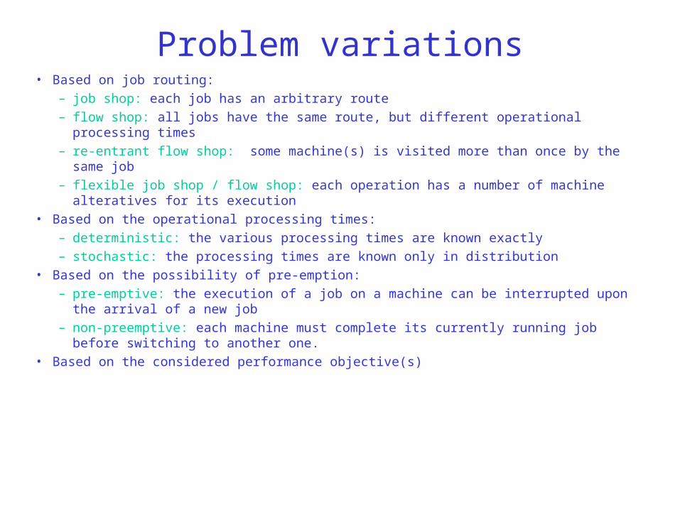
Problem variations• Based on job routing:

– job shop: each job has an arbitrary route

– flow shop: all jobs have the same route, but different operational processing times

– re-entrant flow shop: some machine(s) is visited more than once by the same job

– flexible job shop / flow shop: each operation has a number of machine alteratives for its execution

• Based on the operational processing times:

– deterministic: the various processing times are known exactly

– stochastic: the processing times are known only in distribution

• Based on the possibility of pre-emption:

– pre-emptive: the execution of a job on a machine can be interrupted upon the arrival of a new job

– non-preemptive: each machine must complete its currently running job before switching to another one.

• Based on the considered performance objective(s)

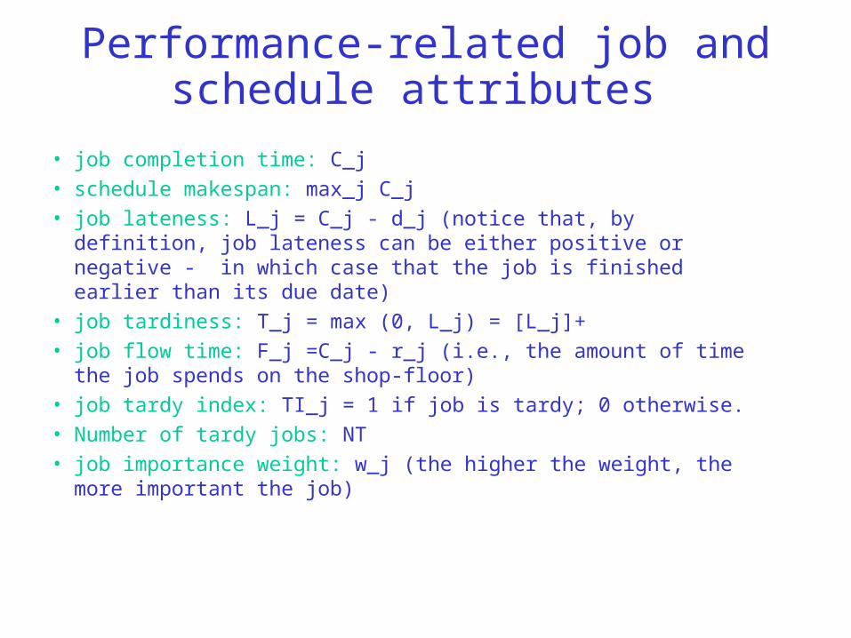
Performance-related job and schedule attributes

• job completion time: C_j

• schedule makespan: max_j C_j

• job lateness: L_j = C_j - d_j (notice that, by definition, job lateness can be either positive or negative - in which case that the job is finished earlier than its due date)

• job tardiness: T_j = max (0, L_j) = [L_j]+

• job flow time: F_j =C_j - r_j (i.e., the amount of time the job spends on the shop-floor)

• job tardy index: TI_j = 1 if job is tardy; 0 otherwise.

• Number of tardy jobs: NT

• job importance weight: w_j (the higher the weight, the more important the job)

Performance Criteria

Job Attribute min total min weighted total min max min weighted maxLateness _j L_j _j w_j*L_j max_j L_j max_j w_j*L_jTardiness _j T_j _j w_j*T_j max_j T_j max_j w_j*T_jFlow time _j F_j _j w_j*F_j max_j F_j max_j w_j*F_j

Tardy index NTCompletion _j C_j _j w_j*C_j max_j C_j max_j w_j*C_j

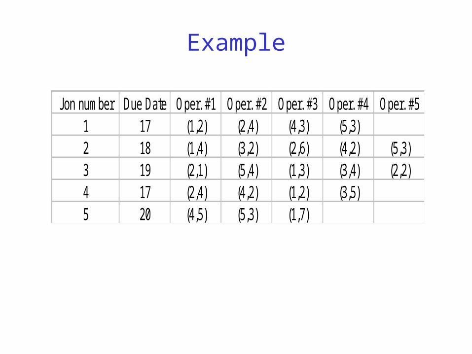
Example

Jon number Due Date Oper. #1 Oper. #2 Oper. #3 Oper. #4 Oper. #51 17 (1,2) (2,4) (4,3) (5,3)2 18 (1,4) (3,2) (2,6) (4,2) (5,3)3 19 (2,1) (5,4) (1,3) (3,4) (2,2)4 17 (2,4) (4,2) (1,2) (3,5)5 20 (4,5) (5,3) (1,7)

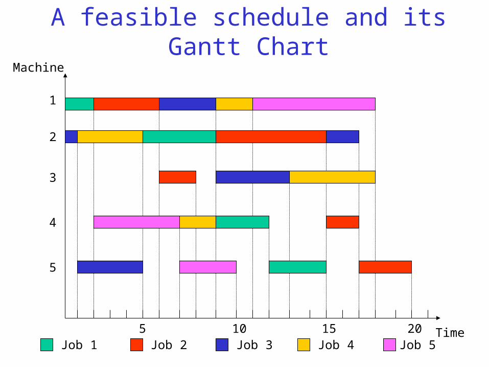
A feasible schedule and its Gantt Chart

1

2

3

4

5

5 10 15 20

Machine

TimeJob 1 Job 2 Job 3 Job 4 Job 5

Schedule Performance Evaluation

Job d_j C_j F_j L_j T_j TI_j1 17 15 15 -2 0 02 18 20 20 2 2 13 19 17 17 -2 0 04 17 18 18 1 1 15 20 18 18 -2 0 0

Total 88 88 -3 3 2average 17.6 17.6 -0.6 0.6

max 20 20 2 2

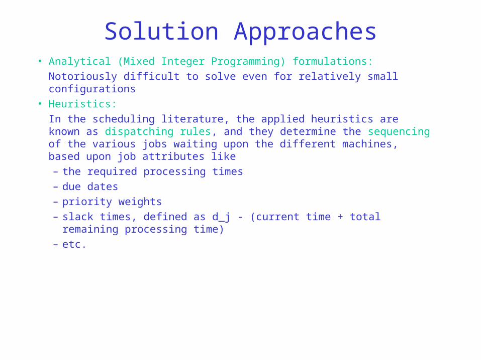
Solution Approaches• Analytical (Mixed Integer Programming) formulations:

Notoriously difficult to solve even for relatively small configurations

• Heuristics:

In the scheduling literature, the applied heuristics are known as dispatching rules, and they determine the sequencing of the various jobs waiting upon the different machines, based upon job attributes like

– the required processing times

– due dates

– priority weights

– slack times, defined as d_j - (current time + total remaining processing time)

– etc.

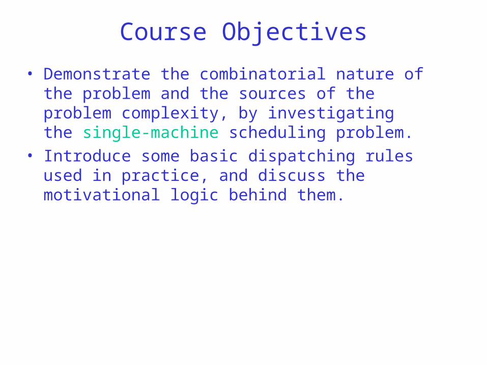
Course Objectives

• Demonstrate the combinatorial nature of the problem and the sources of the problem complexity, by investigating the single-machine scheduling problem.

• Introduce some basic dispatching rules used in practice, and discuss the motivational logic behind them.

Production Planning & Scheduling in Large Corporations.

Documents

Transcript of Production Planning & Scheduling in Large Corporations.