Producer Theory

Production

ASSUMPTION 2.1 Properties of the Production Set The production set Y satisfies the following properties

1. Y is non-empty If Y is empty, we have nothing to talk about 2. Y is closed A set is closed if it contains its boundary. We need this for the solution existence in the profit maximization problem. 3. No free lunch You cannot produce output without using any inputs. In other words, any feasible production plan y must have at least one negative component. 4. Free disposal The firm can always throw away inputs for free. For any point in Y, points that use less of all components are also in Y. Thus if y Y∈ , any point below and to the left is also in Y (in the two dimensional model). This is mostly a technical assumption and ensures that Y is not bounded below which has something to do with the second-order conditions in the profit maximizing problem.

Production

ASSUMPTION 2.2 Properties of the production function

The production function : nf + +→ is continuous, strictly increasing and strictly

quasiconcave on n+ , and (0) 0f = .

Elasticity of Substitution

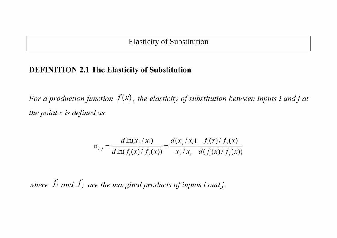
DEFINITION 2.1 The Elasticity of Substitution

For a production function ( )f x , the elasticity of substitution between inputs i and j at

the point x is defined as

,

ln( / ) ( / ) ( ) / ( )ln( ( ) / ( )) / ( ( ) / ( ))

j i j i i ji j

i j j i i j

d x x d x x f x f xd f x f x x x d f x f x

σ = =

where if and jf are the marginal products of inputs i and j.

ΤΗΕΟREM 2.1 Linear Homogeneous Production Functions are Concave

Let : nf + +→ be a continuous, increasing and quasiconcave production function,

with f(0) = 0. Suppose f(.) is homogeneous of degree 1. Then f(.) is a concave function.

Returns to scale

DEFINITION 2.2 (Global) Returns to Scale

Α production function f(x) has the property of

1. CRS if ( ) ( ), 0,f tx tf x t x= ∀ > ∀

2. IRS if ( ) ( ), 1,f tx tf x t x> ∀ > ∀

3. DRS if ( ) ( ), 1,f tx tf x t x< ∀ > ∀

Local Returns to scale

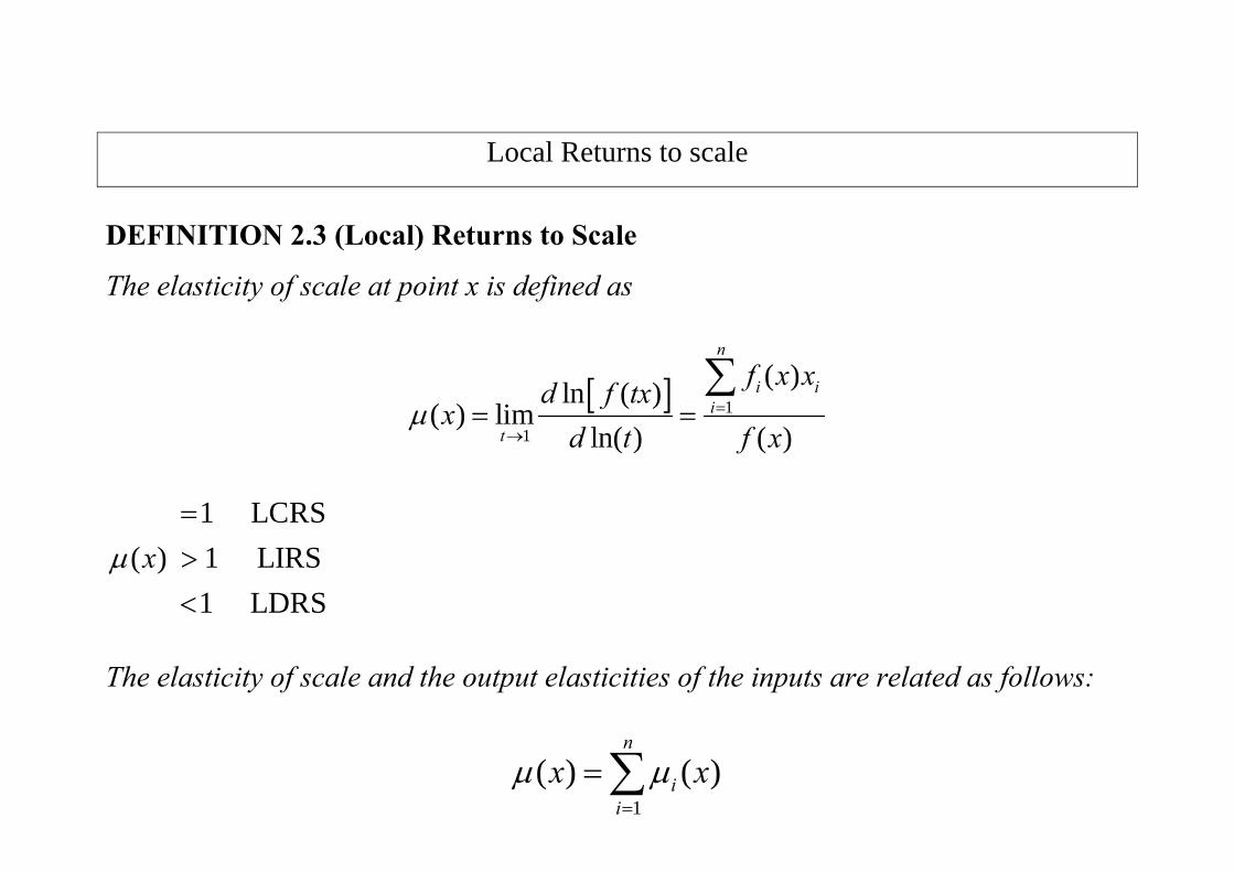
DEFINITION 2.3 (Local) Returns to Scale

The elasticity of scale at point x is defined as

[ ] 1

1

( )ln ( )( ) lim

ln( ) ( )

n

i ii

t

f x xd f txx

d t f xμ =

→= =

∑

1 LCRS

( ) 1 LIRS1 LDRS

xμ=><

The elasticity of scale and the output elasticities of the inputs are related as follows:

1( ) ( )

n

ii

x xμ μ=

=∑

Homothetic Function

DEFINITION 2.3 Homothetic Function

Α homothetic function is a positive monotonic transformation of a function

that is homogeneous of degree 1.

COST

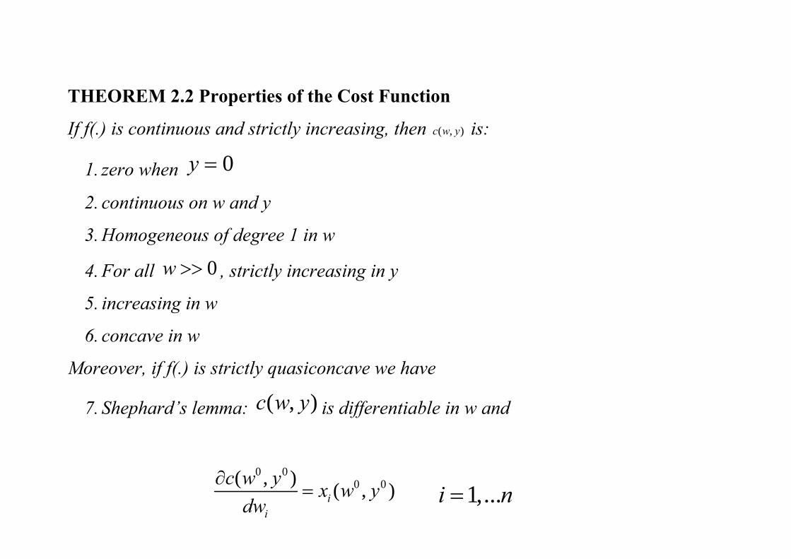
ΤΗΕΟREM 2.2 Properties of the Cost Function

If f(.) is continuous and strictly increasing, then ( , )c w y is:

1. zero when 0y =

2. continuous on w and y

3. Homogeneous of degree 1 in w

4. For all 0w >> , strictly increasing in y

5. increasing in w

6. concave in w

Moreover, if f(.) is strictly quasiconcave we have

7. Shephard’s lemma: ( , )c w y is differentiable in w and

0 00 0( , ) ( , )i

i

c w y x w ydw

∂= 1,...i n=

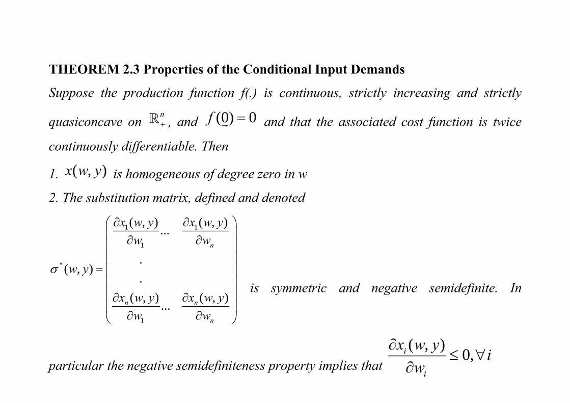
ΤΗΕΟREM 2.3 Properties of the Conditional Input Demands

Suppose the production function f(.) is continuous, strictly increasing and strictly

quasiconcave on n+ , and (0) 0f = and that the associated cost function is twice

continuously differentiable. Then

1. ( , )x w y is homogeneous of degree zero in w

2. The substitution matrix, defined and denoted

1 1

1

*

1

( , ) ( , )...

.( , )

.( , ) ( , )...

n

n n

n

x w y x w yw w

w y

x w y x w yw w

σ

∂ ∂⎛ ⎞⎜ ⎟∂ ∂⎜ ⎟⎜ ⎟

= ⎜ ⎟⎜ ⎟⎜ ⎟∂ ∂⎜ ⎟

∂ ∂⎝ ⎠

is symmetric and negative semidefinite. In

particular the negative semidefiniteness property implies that ( , ) 0,i

i

x w y iw

∂≤ ∀

∂

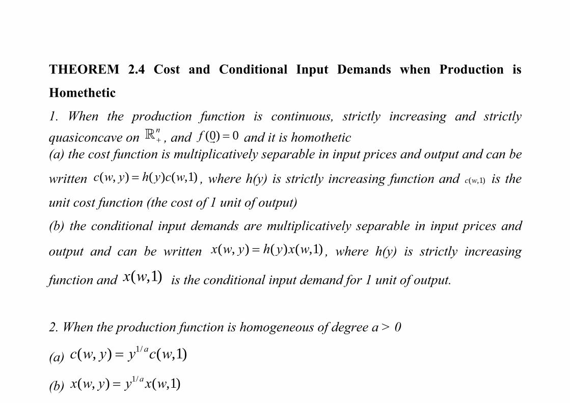
ΤΗΕΟREM 2.4 Cost and Conditional Input Demands when Production is

Homethetic

1. When the production function is continuous, strictly increasing and strictly quasiconcave on

n+ , and (0) 0f = and it is homothetic

(a) the cost function is multiplicatively separable in input prices and output and can be

written ( , ) ( ) ( ,1)c w y h y c w= , where h(y) is strictly increasing function and ( ,1)c w is the

unit cost function (the cost of 1 unit of output)

(b) the conditional input demands are multiplicatively separable in input prices and

output and can be written ( , ) ( ) ( ,1)x w y h y x w= , where h(y) is strictly increasing

function and ( ,1)x w is the conditional input demand for 1 unit of output.

2. When the production function is homogeneous of degree a > 0

(a) 1/( , ) ( ,1)ac w y y c w=

(b) 1/( , ) ( ,1)ax w y y x w=

DEFINITION 2.4 The Short-Run Cost Function

Let the production function be ( , )f x x . Suppose that x is a subvector of variable

inputs and x is a subvector of fixed inputs. Let w and w be the associated input

prices for the variable and fixed inputs, respectively. The short-run total cost function

is defined as

( , , ; ) min . . ( , )x

sc w w y x wx wx s t f x x y≡ + ≥

If ( , , ; )x w w y x solves this minimization problem, then

total fixed costtotal variable cost

( , , ; ) ( , , ; ) sc w w y x wx w w y x wx≡ +

THE COMPETITIVE FIRM

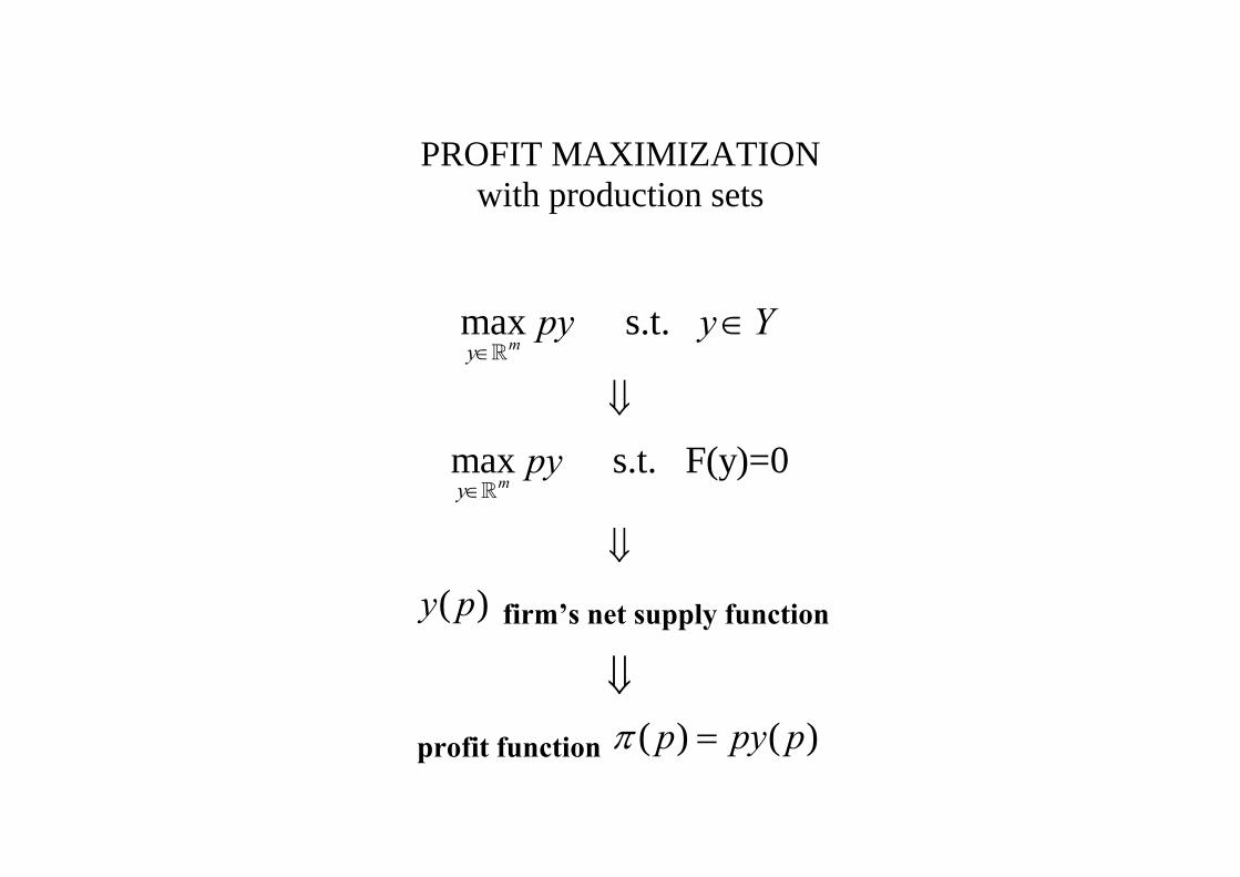
PROFIT MAXIMIZATION with production sets

max s.t. my

py y Y∈

∈

⇓

max s.t. F(y)=0my

py∈

⇓

( )y p firm’s net supply function

⇓

profit function ( ) ( )p py pπ =

PROFIT MAXIMIZATION with production sets

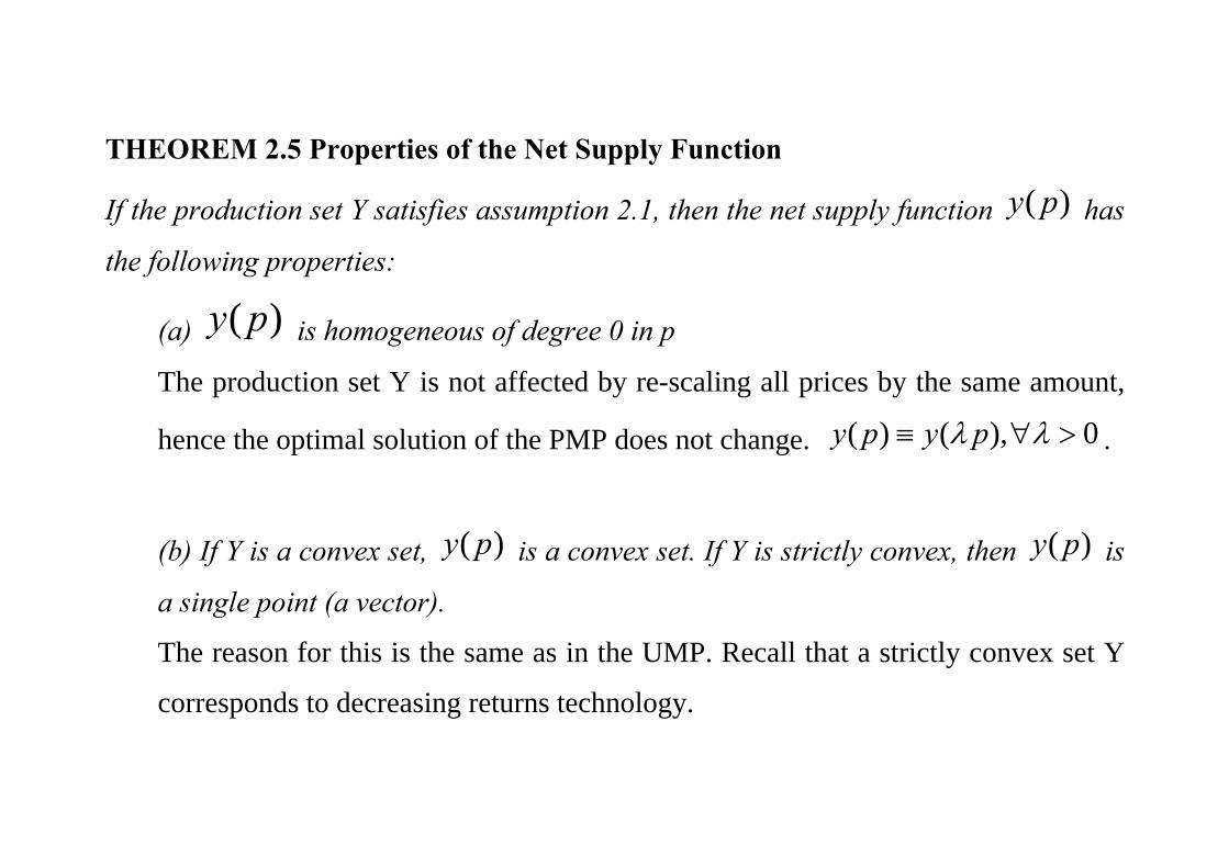
ΤΗΕΟREM 2.5 Properties of the Net Supply Function

If the production set Y satisfies assumption 2.1, then the net supply function ( )y p has

the following properties:

(a) ( )y p is homogeneous of degree 0 in p

The production set Y is not affected by re-scaling all prices by the same amount,

hence the optimal solution of the PMP does not change. ( ) ( ), 0y p y pλ λ≡ ∀ > .

(b) If Y is a convex set, ( )y p is a convex set. If Y is strictly convex, then ( )y p is

a single point (a vector).

The reason for this is the same as in the UMP. Recall that a strictly convex set Y

corresponds to decreasing returns technology.

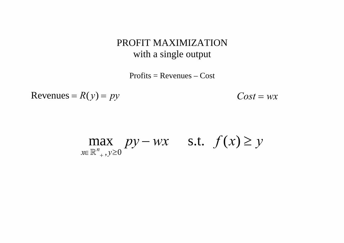
PROFIT MAXIMIZATION with a single output

Profits = Revenues – Cost

Revenues ( )R y py= = Cost wx=

, 0max s.t. ( )

nx ypy wx f x y

+∈ ≥− ≥

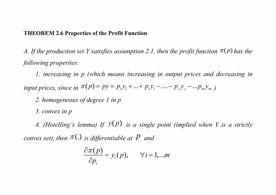
ΤΗΕΟREM 2.6 Properties of the Profit Function

A. If the production set Y satisfies assumption 2.1, then the profit function ( )pπ has the

following properties:

1. increasing in p (which means increasing in output prices and decreasing in

input prices, since in 1 1( ) ... .... ...i i j j m mp py p y p y p y p yπ = = + + − − − )

2. homogeneous of degree 1 in p

3. convex in p

4. (Hotelling’s lemma) If ( )y p is a single point (implied when Y is a strictly

convex set), then (.)π is differentiable at p and

( ) ( ), 1,...i

i

p y p i mp

π∂= ∀ =

∂

B. If the production function f(.) satisfies assumption 2.2, then the profit function

( , )p wπ , where well-defined, is continuous and

1. increasing in p and decreasing in w

2. homogeneous of degree 1 in (p,w)

3. convex in (p,w)

4. differentiable in (p,w). Moreover,

( , ) ( , )

( , ) ( , ) 1,...,ii

p w y p wpp w x p w i nw

π

π

∂=

∂∂

= − ∀ =∂

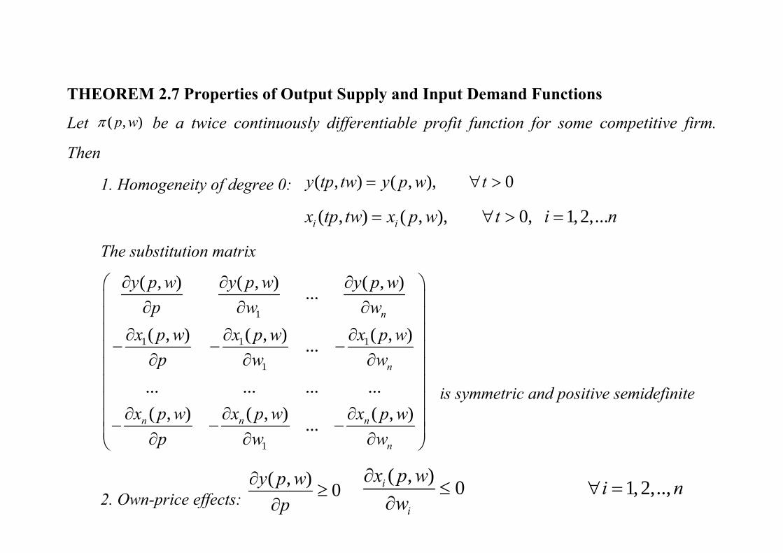
ΤΗΕΟREM 2.7 Properties of Output Supply and Input Demand Functions

Let ( , )p wπ be a twice continuously differentiable profit function for some competitive firm.

Then

1. Homogeneity of degree 0: ( , ) ( , ), 0y tp tw y p w t= ∀ >

( , ) ( , ), 0, 1, 2,...i ix tp tw x p w t i n= ∀ > =

The substitution matrix

1

1 1 1

1

1

( , ) ( , ) ( , )...

( , ) ( , ) ( , )...

... ... ... ...( , ) ( , ) ( , )...

n

n

n n n

n

y p w y p w y p wp w w

x p w x p w x p wp w w

x p w x p w x p wp w w

∂ ∂ ∂⎛ ⎞⎜ ⎟∂ ∂ ∂⎜ ⎟⎜ ⎟∂ ∂ ∂− − −⎜ ⎟∂ ∂ ∂⎜ ⎟

⎜ ⎟⎜ ⎟

∂ ∂ ∂⎜ ⎟− − −⎜ ⎟∂ ∂ ∂⎝ ⎠

is symmetric and positive semidefinite

2. Own-price effects: ( , ) 0y p w

p∂

≥∂

( , ) 0 1, 2,..,i

i

x p w i nw

∂≤ ∀ =

∂

ΤΗΕΟREM 2.8 The Short-Run Profit Function

Let the production function be ( , )f x x , where x is a subvector of variable inputs and x is a

subvector of fixed inputs. Let w and w be the associated input prices for variable and fixed

inputs, respectively. The short run, profit function is defined as

,( , , , ) max s.t. ( , )

y xp w w x py wx wx f x x yπ ≡ − − ≥

The solutions ( , , , )y p w w x and ( , , , )x p w w x are called the short-run output supply and

variable input demand functions, respectively.

For all 0p > and 0w >> , ( , , , )p w w xπ where well-defined is continuous in p and w,

increasing in p, decreasing in w, and convex in (p,w). If ( , , , )p w w xπ is twice continuously

differentiable, ( , , , )y p w w x and ( , , , )x p w w x possess all three properties listed in

Theorem 2.7 with respect to output and variable input prices.