Process integration study of a biorefinery producing...

Process integration study of a biorefinery

producing ethylene from lignocellulosic

feedstock for a chemical cluster Master’s Thesis within the Innovative and Sustainable Chemical Engineering

programme

MARIA ARVIDSSON

BJÖRN LUNDIN

Department of Energy and Environment

Division of Heat and Power Technology

CHALMERS UNIVERSITY OF TECHNOLOGY

Göteborg, Sweden 2011

MASTER’S THESIS

Process integration study of a biorefinery producing

ethylene from lignocellulosic feedstock for a chemical

cluster

Master’s Thesis within the Innovative and Sustainable Chemical Engineering

programme

MARIA ARVIDSSON

BJÖRN LUNDIN

SUPERVISORS

Roman Hackl

Reine Spetz

EXAMINER

Simon Harvey



CHALMERS UNIVERSITY OF TECHNOLOGY


Process integration study of a biorefinery producing ethylene from lignocellulosic

feedstock for a chemical cluster

Master’s Thesis within the Innovative and Sustainable Chemical Engineering

programme

MARIA ARVIDSSON

BJÖRN LUNDIN

© MARIA ARVIDSSON, BJÖRN LUNDIN, 2011



Chalmers University of Technology

SE-412 96 Göteborg

Sweden

Telephone: + 46 (0)31-772 1000

Chalmers Reproservice


I

Process integration study of a biorefinery producing ethylene from lignocellulosic

feedstock for a chemical cluster

Master’s Thesis in the Innovative and Sustainable Chemical Engineering programme

MARIA ARVIDSSON

BJÖRN LUNDIN



Chalmers University of Technology

ABSTRACT

A chemical cluster producing a variety of products is situated in Stenungsund,

Sweden. In 2010 the ethylene consumption of the cluster (currently covered by import

and a steam cracker converting e.g. naphta) increased due to the start-up of a new

polyethylene (PE) plant by Borealis AB. This work investigates the opportunity to

cover the current ethylene import (i.e. 200 000 tonnes/year) by the introduction of a

biorefinery plant (reducing fossil fuel dependence and greenhouse gas (GHG)

emissions from the cluster). High material and energy efficiency is of utmost

importance to achieve economic competitiveness. Hence, heat integration is essential.

A simulation model for a biorefinery is established in Aspen Plus based on literature

review and personal contacts with experts. A process integration study is conducted

using pinch analysis of simulation results. The aim is to investigate the integration

consequences (e.g. potential energy savings and economical aspects) of combining a

stand-alone lignocellulosic ethanol and a stand-alone ethanol dehydration plant into a

biorefinery producing ethylene from lignocellulosic feedstock via the fermentation

route. Several process configurations of the biorefinery are investigated, e.g. the

integration of the biorefinery with the existing cluster based on results obtained from a

total site analysis (TSA) (Hackl, et al., 2010).

In the lignocellulosic ethanol production spruce (749 MW) is converted to ethanol

(337 MW) and a lignin-rich co-product (370 MW), which can be utilised as fuel in a

combined heat and power (CHP) plant supplying steam (for hot utility and direct

injection into process streams) and electricity. The stand-alone ethanol plant results in

excess solid residues (86 MW) and electricity (24 MWel). In the ethylene production,

ethanol (337 MW) is converted to ethylene (307 MW). The stand-alone ethylene plant

requires external fuel (16 MW) to cover hot utility demand. Moreover, electricity

(4 MWel) and steam for direct injection (25 MW) must be produced externally. The

results indicate that energy savings (40% and 28% reduction of minimum hot and cold

utility respectively) can be achieved by integrating the two stand-alone processes into

a biorefinery. Moreover, the integration opportunity to eliminate external fuel, steam

and electricity requirements by firing of excess solid residues arises. It is shown that

the minimum hot utility demand can be further reduced by 59% by introducing a

MVR in the biorefinery (Bio-MVR), which corresponds to a 75% reduction compared

with the two stand-alone processes. The results show that the excess solid residues of

the biorefinery can eliminate the external fuel requirement by flue gas integration or

deliver VHP (41 bar) steam to the existing cluster. The lowest ethylene production

cost (1.0 €/kg ethylene) is obtained for the Bio-MVR.

Key words: heat integration, process integration, pinch analysis, chemical cluster,

biorefinery, bioethylene, lignocellulosic ethanol, fermentation route, Aspen Plus

III

Contents

ABSTRACT I

CONTENTS III

PREFACE VII

NOTATIONS VIII

1 INTRODUCTION 1

1.1 Objective 2

2 BACKGROUND 5

2.1 Stand-alone lignocellulosic ethanol production 5 2.1.1 Renewable raw material 5 2.1.2 Stand-alone lignocellulosic ethanol production configuration 7 2.1.3 Pretreatment 9

2.1.4 Hydrolysis 12 2.1.5 Fermentation 13

2.1.6 Product purification 14 2.1.7 Evaporation 15 2.1.8 Recirculation of process streams 15

2.1.9 Combined Heat and Power (CHP) plant 16 2.1.10 Wastewater treatment (WWT) 16

2.2 Stand-alone ethanol dehydration to ethylene production 16

2.2.1 Stand-alone ethanol dehydration to ethylene production configuration

16 2.2.2 Reactor 18

2.2.3 Quench tower 20 2.2.4 Compressor 20 2.2.5 Caustic tower 20

2.2.6 Dryer 20 2.2.7 Ethylene column and stripper 21

2.3 Biorefinery - Ethylene production from lignocellulosic feedstock 21

2.4 Chemical cluster 23

3 METHODOLOGY 25

3.1 Stand-alone lignocellulosic ethanol production simulations in Aspen Plus 25 3.1.1 Components 25

3.1.2 Pretreatment 26 3.1.3 Simultaneous Saccharification and Co-Fermentation (SSCF) 27 3.1.4 Product purification 28

3.1.5 Evaporation 29 3.1.6 Combined Heat and Power (CHP) plant 30

3.2 Stand-alone ethanol dehydration to ethylene production simulations in

Aspen Plus 31

IV

3.2.1 Components 31 3.2.2 Adiabatic reactor 32 3.2.3 Quench tower 33

3.2.4 Compressor 34 3.2.5 Caustic tower 34 3.2.6 Dryer 35 3.2.7 Ethylene column and stripper 35

3.3 Biorefinery - Ethylene production from lignocellulosic feedstock

simulations in Aspen Plus 36 3.3.1 Configuration of rectifier column 36 3.3.2 Configuration of ethanol dehydration to ethylene reactor 36 3.3.3 Configuration of CHP plant 37

3.4 Pinch technology 38

3.5 Economic evaluation 40 3.5.1 Total capital cost estimation 41 3.5.2 Operating costs estimation 42

3.5.3 Production cost estimation 43

4 RESULTS AND DISCUSSION 45

4.1 Simulation results 45 4.1.1 Stand-alone lignocellulosic ethanol production 45

4.1.2 Stand-alone ethanol dehydration to ethylene production 46

4.2 Heat integration results 48

4.2.1 Stand-alone lignocellulosic ethanol production 48

4.2.2 Stand-alone ethanol dehydration to ethylene production 49

4.2.3 Background/foreground analysis of the stand-alone lignocellulosic

ethanol production and the stand-alone ethanol dehydration to ethylene

production 51 4.2.4 Biorefinery - Ethylene production from lignocellulosic feedstock 52

4.2.5 Alternative biorefinery configurations 55 4.2.6 Biorefinery – Flue gas integration with ethylene reactors (Bio-F) 57 4.2.7 Biorefinery – Introduction of MVR on the rectifier distillate

(Bio-MVR) 60 4.2.8 Biorefinery – VHP (41 bar) steam delivery to the chemical cluster

(Bio-VHP) 62 4.2.9 Summary of heat integration results 64

4.3 Economic evaluation 65 4.3.1 Total capital cost estimation 65 4.3.2 Annual operating cost estimation 67 4.3.3 Annual revenue estimation 69 4.3.4 Production cost estimation 71

5 CONCLUSION 75

6 FURTHER WORK 77

6.1 Flue gas integration with ethylene reactors 77

V

6.2 Integration opportunities with the chemical cluster 77

6.3 District heating 77

6.4 Sustainable ethylene? 78

7 REFERENCES 79

APPENDIX A: ALTERNATIVE PRETREATMENT METHODS 85

APPENDIX B: USER DEFINED COMPONENTS – INPUT DATA 86

APPENDIX C: STAND-ALONE ETHANOL FROM LIGNOCELLULOSIC

FEEDSTOCK PRODUCTION - REACTIONS 87

APPENDIX D: STAND-ALONE ETHANOL DEHYDRATION TO ETHYLENE

PRODUCTION - REACTIONS 90

APPENDIX E: STREAM DATA FOR THE STAND-ALONE LIGNOCELLULOSIC

ETHANOL PRODUCTION 91

APPENDIX F: STREAM DATA FOR THE STAND-ALONE ETHANOL

DEHYDRATION TO ETHYLENE PRODUCTION 92

APPENDIX G: STREAM DATA FOR THE BIOREFINERY – ETHYLENE FROM

LIGNOCELLULOSIC FEEDSTOCK PRODUCTION 93

APPENDIX H: STREAM DATA FOR THE BIO-MVR 94

APPENDIX I: EQUIPMENT COSTS FOR INDIVIDUAL UNIT OPERATIONS IN

THE LIGNOCELLULOSIC ETHANOL PRODUCTION 95

APPENDIX J: EQUIPMENT COSTS FOR THE CHP PLANT AND THE MVR

HEAT PUMP 98

APPENDIX K: EXCHANGE RATES 96

VII

Preface

This study investigates the opportunity to substitute current ethylene import,

originating from fossil resources, of the chemical cluster located in Stenungsund with

a biorefinery producing ethylene from lignocellulosic feedstock.

This Master’s thesis has been carried out at the Department of Energy and

Environment, Division of Heat and Power Technology, Chalmers University of

Technology, Sweden.

We would like to thank our examiner, Professor Simon Harvey, for showing support

and interest in our work, and for valuable input on the report. We would also like to

thank our supervisor at Borealis AB, Reine Spetz, for making this project possible, for

showing interest, and for giving useful comments on the work. We would also like to

thank our supervisor at the Division of Heat and Power Technology, Roman Hackl,

for giving us encouragement and support during the project.

Thank you, Åsa Lindqvist and Christoffer Johansson, for reviewing and commenting

on the report.

We would like to give special thanks to Lic. Eng. Rickard Fornell at the Division of

Heat and Power Technology, Chalmers University of Technology for giving us useful

information about the ethanol production process and for providing help and support

concerning Aspen Plus simulations.

We would also give special thanks to Associate Professor Carl Johan Franzén at the

Department of Chemical and Biological Engineering, Chalmers University of

Technology for rewarding discussions regarding hydrolysis and fermentation.

Göteborg April 2011

Maria Arvidsson

Björn Lundin

VIII

Notations

Abbreviations

BG/FG Background/foreground

BOD7 Biological oxygen demand

C5 Pentose

C6 Hexose

CC Composite curve

CE Chemical engineering

CHP Combined heat and power

COD Chemical oxygen demand

COP Coefficient of performance

CW Cooling water

DM Dry matter

ELECNRTL Electrolyte Non-Random Two Liquids

ETBE Ethyl tert-butyl ether

EtOH Ethanol

FEHX Feed-effluent heat exchanger

GCC Grand composite curve

GHG Greenhouse gas

HEX Heat exchange

HHV High heating values

HMF 5-hydroxymethylfurfural

HP High pressure steam 20 bar (absolute pressure)

LP Low pressure steam 4 bar (absolute pressure)

MP Medium pressure steam 13 bar (absolute pressure)

MVR Mechanical vapor recompression

NPV Net present value

NREL National Renewable Energy Laboratory

NRTL Non-Random Two Liquids

PE Polyethylene

SHCF Separate hydrolysis and co-fermentation

SHF Separate hydrolysis and fermentation

SSCF Simultaneous saccharification and co-fermentation

SSF Simultaneous saccharification and fermentation

IX

TSA Total site analysis

VHP Very high pressure steam 41 bar (absolute pressure)

WIS Water insoluble solids

WWT Waste water treatment

Symbols

Equipment cost for capacity

Wel Electrical work

QC,min Minimum cold utility demand

QC,Refrig Refrigeration utility demand

QDH District heating potential

QH,furnace Hot utility demand covered by furnace

QH,LP steam LP steam utility demand

QH,min Minimum hot utility demand

QH,utility Hot utility demand

QREC Maximum heat recovery through internal heat exchange

QH,VHP steam Very high pressure steam utility demand

Tpinch Pinch temperature

ΔTmin Minimum temperature difference

€ Euro

1

1 Introduction

Depleting crude oil reservoirs, climate change due to greenhouse gas (GHG)

emissions, a growing population with an increased energy and material demand have

driven the interest in finding sustainable alternatives to the fossil feedstock dependent

markets forward. One potential alternative is the biorefinery concept, which converts

biomass to e.g. fuels, energy, and value-added chemicals. This implies that renewable

feedstock is used for products that are traditionally produced from fossil raw material,

thereby reducing fossil fuel dependence and GHG emissions. The biorefinery concept

will play an important role in achieving a sustainable future society, where energy and

material are less fossil fuel dependent.

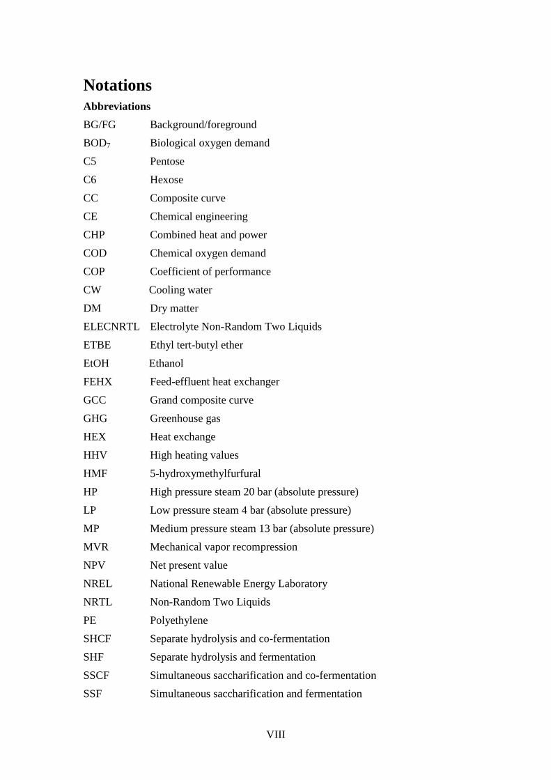
In Stenungsund, Sweden, a chemical cluster consisting of five sites producing a variety

of different products is situated, see Figure 1.1. One of the sites, Borealis AB, produces

polyethylene (PE) (700 ktonnes annually (Borealis AB, 2010)) for mainly wire and

cable and pipe applications. In 2010 Borealis AB invested in a new high pressure

polyethylene (PE) plant which increased the annual production of PE and therefore

also the ethylene consumption.

Figure 1.1 Material flows in the chemical cluster in Stenungsund (Borealis AB,

2007).

The current ethylene demand of the cluster is supplied by import (approximately 1/3 of

the total ethylene demand) and a steam cracker (approximately 2/3 of the total ethylene

demand). The steam cracker converts naphtha, ethane, propane and other raw materials

to e.g. ethylene and propylene, see Table 1.1. The introduction of a biorefinery,

producing bioethylene from renewable raw material, is one opportunity to cover the

increased ethylene demand and consequently reducing the fossil feedstock dependence

of the chemical cluster.

2

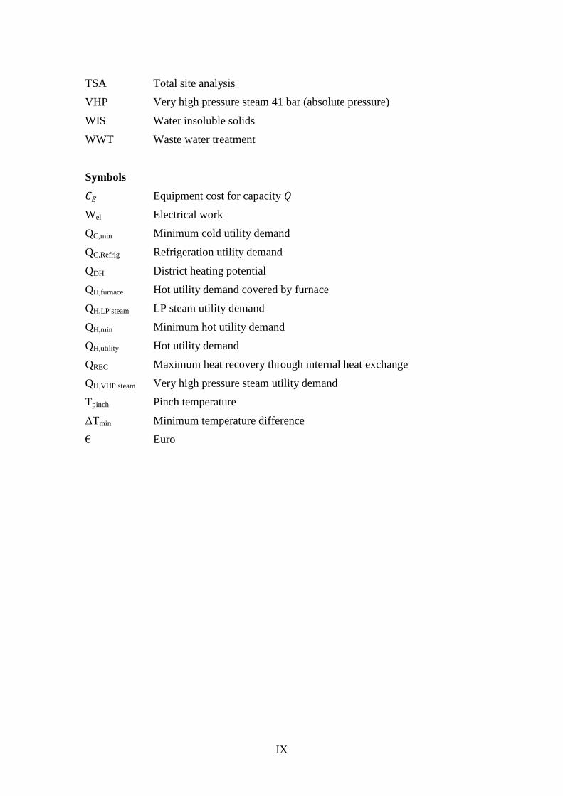
Table 1.1 Annual raw material consumption (left) and annual production (right)

of the steam cracker in Stenungsund (Borealis AB, 2007).

Raw material

consumption

ktonne Production ktonne

Naphta 360 Ethylene 622

Ethane 358 Propylene 200

Propane 246 Others 488

Buthane

Ethanol

368

12 Ethyl tert-butyl ether (ETBE) 28

Ethylene can be produced via several alternative routes from biomass. One route is

hydrolysis of biomass into monomeric sugars which are further converted to ethanol by

fermentation. Ethylene is thereafter produced through catalytic dehydration of ethanol.

An alternative route is gasification of biomass producing syngas. From syngas,

methanol is generated which is further converted to olefins (mainly ethylene and

propylene). A full-scale (production capacity of 200 000 tonnes annually) polyethylene

production site from sugarcane based feedstock was started up in Brazil 2010 by

Braskem (Braskem, 2010). The technology is expected to reach Europe when ethanol

production from lignocellulosic feedstock is economically competitive.

To enable competition with well-established petroleum based processes it is of utter

importance to achieve high energy and material efficiency for the biorefinery. To

increase the thermal efficiency heat integration is essential. Available process heat

sources are then used to cover heat sinks, reducing the demand of external utilities.

Heat integration can be conducted internally in processes by heat exchanging of

streams having excess of heat with streams having heat deficits. Heat integration can

also be conducted between industries in chemical clusters by e.g. heat exchanging and

implementation of common utility systems. When implementing process integration

between neighbouring sites, it is also important to identify opportunities for

exchanging materials, taking advantage of already existing infrastructure.

1.1 Objective

The aim of the thesis, Process integration study of a biorefinery producing ethylene

from lignocellulosic feedstock for a chemical cluster, is to establish a simulation model

for a biorefinery producing ethylene from lignocellulosic feedstock via the

fermentation route. The bioethylene production is assumed to cover the current

ethylene import of the chemical cluster, i.e. 200 000 tonnes annually. The simulation

model is based on process design of a biorefinery configuration gathered from an

extensive literature study and personal contact with experts.

The second objective is to investigate the heat integration potential of a stand-alone

lignocellulosic ethanol production plant and a stand-alone catalytic ethanol dehydration

plant producing ethylene. The consequences (e.g. potential energy savings and

economical aspects) of combining a lignocellulosic ethanol production plant and an

ethylene production plant into an integrated biorefinery producing ethylene from

lignocellulosic feedstock are investigated. Moreover, the aim of the thesis is to

3

investigate the effects of integrating the proposed biorefinery (ethylene production

from lignocellulosic feedstock) with the existing industrial cluster in Stenungsund,

through exchange of steam with the chemical cluster at suitable pressure levels.

Different process configurations of the combined biorefinery are compared. Effects

investigated from an energy perspective are e.g. heat integration potential and

consequently minimum hot and cold utility demand, co-product (e.g. lignin-rich solid

residue from the ethanol production plant) utilisation to reduce/cover the hot utility

demand, and electricity production. The process integration is performed using pinch

analysis. Relevant process information, i.e. heat sources and sinks in the biorefinery

are identified by Aspen Plus simulations of the processes. Results from a total site

analysis (TSA) are used concerning heat integration opportunities with the chemical

cluster (Hackl, et al., 2010).

Additionally, the economical effects of producing ethylene from lignocellulosic

feedstock in a biorefinery are investigated and compared with the case of purchasing

ethanol to a stand-alone ethylene production plant.

5

2 Background

Ethylene production from lignocellulosic feedstock basically consists of two separate

processes: ethanol production from lignocellulosic raw material (i.e. stand-alone

lignocellulosic ethanol production) and catalytic dehydration of ethanol forming

ethylene (i.e. stand-alone ethanol dehydration to ethylene production). The

combination of these two processes is referred to as the biorefinery in this report.

2.1 Stand-alone lignocellulosic ethanol production

2.1.1 Renewable raw material

The conversion of carbohydrates into ethanol is a well-known process. Ethanol has

traditionally been produced from sugar-based (e.g. sugar cane and sugar beet) or

starch-based (e.g. corn and wheat) materials. However, in order to meet increasing

future demands and to avoid direct competition with food production, the development

of ethanol production processes using lignocellulosic feedstock is of utter importance

to reach a sustainable society. Figure 2.1 shows an overview of required process steps

for ethanol production from different raw materials.

Figure 2.1 Overview of required process steps for bioethanol production for

different feedstocks.

As can be seen in Figure 2.1 it is far easier to achieve fermentable monomeric sugars

from sugar- and starch-based materials compared to lignocellulosic materials. When

producing ethanol from sugar-based raw material the sugars (in the form of sucrose)

are fermentable without any pretreatment or hydrolysis. Using starch-based material

hydrolysis is required before fermentation is possible. Ethanol production from

lignocellulosic raw material requires both pretreatment and hydrolysis prior to

fermentation. Examples of lignocellulosic materials are softwood (e.g. spruce),

6

hardwood (e.g. salix), and agricultural residues (e.g. corn stover). Lignocellulosic

materials are explained in more detail in Section 2.1.1.1.

In order to achieve an economically competitive ethanol production the raw material

cost must be kept low. Together with the enzyme cost, the cost of biomass is the

largest contributor to the total ethanol production cost (Gregg, et al., 1998). The cost

for lignocellulosic material is comparatively low which makes it attractive as ethanol

production feedstock. In several regions in the world the availability of lignocellulosic

biomass is considered to be sustainable in large quantities (Zhu, et al., 2010). As a

consequence of the significant impact of raw material cost on the total ethanol

production cost, complete and efficient utilisation of the raw material is crucial

(Eriksson, et al., 2010). The fermentable sugars from lignocellulosic feedstock are

comparatively harder to derive, i.e. a pretreatment step is required. In order to attract

industrial interest the cost for deriving fermentable sugars from lignocellulosics needs

to be reduced. When evaluating the bioethanol production cost the overall ethanol yield

is the most important parameter (von Sivers, et al., 1996). In order to improve the

ethanol production economics valuable co-products such as lignin can be utilised (Zhu,

et al., 2010; Sassner, et al., 2008). This is especially true when lignin-rich raw

materials are used. Lignin can be utilised as solid fuel in heat and power generation

and/or sold as product, e.g. pellets.

2.1.1.1 Lignocellulosic feedstock

Lignocellulosic materials consist mainly of cellulose, hemicellulose, and lignin in

different proportions, see Table 2.1. Cellulose is made up of glucan, a crystalline,

linear polysaccharide of linked glucose units. Hemicellulose is an amorphous, highly

branched heterogeneous polysaccharide which consists of glucan, mannan, galactan,

xylan, and arabinan. In other words, hemicellulose consists of units of hexoses

(glucose, mannose, and galactose) and pentoses (xylose and arabinose). Lignin is a

highly complex three-dimensional polymer mainly made up of propylphenol

derivatives.

Table 2.1 Composition (% dry basis) of three different lignocellulosic materials.

(Sassner, et al., 2008)

Spruce Salix Corn stover

Glucan 44.0 42.5 40.0

Mannan 13.0 3.0 -

Galactan 2.3 2.5 2.0

Xylan 6.0 15.0 21.0

Arabinan 2.0 1.5 5.0

Lignin 27.5 26.0 23.0

Acetate 1.3 3.0 1.6

Ash 1.6 2.0 3.5

Others 2.3 4.5 3.9

Hexose (C6) fraction 59.3 48 42

Pentose (C5) fraction 8 16.5 26

7

Mannan dominates the hemicellulose fraction in softwood, while in hardwood and

agricultural residues the hemicellulose is mainly made up of xylan. As a result

softwood has the largest hexose (C6) fraction (59.3%) and the lowest pentose (C5)

fraction (8%) of the three lignocellulosic materials, see Table 2.1. A comparatively

lower fraction of the xylose units are acetylated in softwood. The lignin content of

softwood is generally higher. Additionally lignocellulosics consist of ash. Softwood

has a relatively low ash content (<2%), see Table 2.1. This implies that solid residue

from softwood may have comparatively better fuel properties (Sassner, 2007).

“Others” in Table 2.1 are mainly extractives.

2.1.2 Stand-alone lignocellulosic ethanol production configuration

Ethanol production from lignocellulosic feedstock includes several process steps. In

every process step there are several possible alternatives and a good combination is

required to obtain a cost-effective production. In a future lignocellulosic ethanol

refinery in Sweden, softwood and particularly spruce are considered to be the main

feedstock alternative (Sassner, 2007). Hence, the process configuration of the stand-

alone lignocellulosic ethanol production plant assumed in this study is based on spruce

as main feedstock. However, if commercialising ethanol production from

lignocellulosic feedstock the process must be flexible and universal, i.e. it must be

feedstock versatile and not only effective for one specific species (Zhu, et al., 2010).

Figure 2.2 illustrates an overview of assumed stand-alone lignocellulosic ethanol

production configuration investigated in the study. The assumed process configuration

is based on a literature review. When handling softwood the raw material must first be

debarked and sized. After sizing the wood chips are pretreated to derive the

fermentable hemicellulose sugars and to make cellulose more accessible for hydrolysis.

A two-step dilute acid steam explosion pretreatment is assumed, as a result of mainly

handling softwood feedstock. Direct injection with MP (13 bar) steam (mainly deriving

hemicellulose sugars) and HP (20 bar) steam (mainly making cellulose accessible for

hydrolysis) are assumed in the first and second pretreatment step respectively

(Wingren, et al., 2004). In order to obtain good properties of the solid residue (i.e.

lignin) sulphuric acid is used. An acid concentration of 0.5 wt% and 1 wt% (based on

the water content in feedstock) are assumed in the first and second pretreatment step

respectively (Söderström, et al., 2005). After the first pretreatment step the slurry is

separated into one liquid and one solid fraction in order to reduce hemicellulose sugar

degradation. The filter cake is washed in order to achieve high hemicellulose sugar

recovery. The solid fraction is sent to the second pretreatment step. The pretreatment

step is further explained in Section 2.1.3. The liquid fraction is mixed with the

resulting slurry from the second pretreatment step and flashed down to atmospheric

pressure. The slurry is diluted to 11.2% water insoluble solids (WIS) concentration

(Aden, et al., 2002).

8

Figure 2.2 Stand-alone lignocellulosic ethanol production configuration. SSCF –

Simultaneous Saccharification and Co-Fermentation, (S) – Solid Fraction, (L) – Liquid

Fraction, (C) – Condensate.

In the subsequent hydrolysis (or saccharification) step, cellulose is hydrolysed, i.e.

glucan is converted to glucose, for more details see Section 2.1.4. After pretreatment

and hydrolysis, cellulose and hemicellulose have been converted into their respective

sugars. The hexose sugars are converted to ethanol by the addition of yeast in a

fermentation step. The hydrolysis and fermentation can occur either simultaneously

(SSF) or separately (SHF). If pentose sugar fermentation to ethanol is also occurring it

is referred to as simultaneous saccharification and co-fermentation (SSCF) or separate

hydrolysis and co-fermentation (SHCF). The cellulose hydrolysis is assumed to be

catalysed by enzymes and a futuristic perspective is chosen, thus the ability to ferment

both hexoses and pentoses is presumed (i.e. SSCF configuration). The cellulases and

yeast are assumed to be adapted, i.e. no detoxification step is necessary. Additionally,

enzymes (with a load of 20 kg/t(C5+C6) (Fornell, 2010) and yeast (with addition to a

concentration of 2.5 g/L (Sassner, et al., 2008) are assumed to be purchased. For more

detailed information see Section 2.1.5.

After fermentation ethanol is purified to 93 wt% in several purification steps. The

purification is basically conducted in two steps; one stripper referred to as the beer

column and one distillation column referred to as the rectifier. The fermentation slurry

enters the beer column where unconverted sugars and solids are separated from the

ethanol-water mixture. Additionally, a large fraction of remaining CO2 is removed in

order to enhance the ethanol-water separation in the subsequent purification column

(i.e. the rectifier). For further description see Section 2.1.6.

The resulting bottom product in the beer column is separated into a solid fraction (i.e.

lignin and unconverted wood) and a liquid fraction, see Figure 2.2. The solubilised

non-volatile compounds in the liquid fraction of the beer column stillage are assumed

to be concentrated in a counter-currently arranged five-effect evaporation unit. The

resulting evaporation condensate is suitable as recirculation water reducing fresh water

demand (i.e. wash and dilution water), the remainder is sent to WWT. For more details

9

see Sections 2.1.7 and 2.1.8, respectively. The lignin-rich solid fraction of the beer

column stillage is mixed with the concentrated evaporation syrup and utilised as fuel in

a Combined Heat and Power (CHP) plant supplying steam (for direct steam injection

and as hot utility) and electricity to the process. Possible excess solid residues can be

sold as product, e.g pellets. For more details see Section 2.1.9.

Wastewater generated in the lignocellulosic ethanol production is sent to a wastewater

treatment facility, see Section 2.1.10. However, this is not taken into consideration in

the study.

2.1.3 Pretreatment

The fermentable sugars can be derived from cellulose and hemicellulose through

hydrolysis. However, cellulose, hemicellulose, and lignin are associated in a complex

matrix. The hydrolysis of hemicellulose is relatively easy whereas cellulose is highly

insoluble (Hamelinck, et al., 2005). In order to achieve an efficient hydrolysis of

cellulose the matrix must be modified. This is particularly true for softwood due to its

high lignin content and more rigid structure (Zhu, et al., 2010). Softwood-lignin is

believed to be more branched and non-linear than hardwood-lignin (Gellerstedt, et al.,

2008). Due to the properties concerning lignin and its association to cellulose and

hemicellulose, softwood is more recalcitrant to enzymatic and chemical degradation

(Galbe, et al., 2002; Zhu, et al., 2010). To overcome the recalcitrance and enhance the

cellulose hydrolysis it is necessary to pretreat the feedstock. The hydrolysis yield can

be increased from less than 20% to over 90% if the biomass is pretreated prior to the

hydrolysis step (Hamelinck, et al., 2005). First the feedstock is mechanically

pretreated, i.e. debarked if woody biomass, cleaned if necessary, and sized. Smaller

size results in larger surface area, which is advantageous in the subsequent process

step. However the size is a trade-off with energy usage. The size-reduced feedstock is

then further treated to solubilise hemicellulose and remove lignin in order to make

cellulose accessible for hydrolysis (Galbe, et al., 2002; Zhu, et al., 2010). During

pretreatment hemicellulose is hydrolysed into its respective monomeric or oligomeric

sugar, i.e. mannose is derived from mannan etc. Furthermore a fraction of cellulose is

converted to glucose during pretreatment, even though the main conversion to

monomeric glucose occurs in a separate hydrolysis step, see Section 2.1.4. The derived

sugars may be degraded during pretreatment. The degree of degradation is dependent

on the pretreatment conditions. Higher severity results in higher degree of degradation

(Galbe, et al., 2002). Hexoses are degraded to 5-hydroxymethylfurfural (HMF), and if

further degradation occurs to levulinic and formic acid. Pentose degradation products

are for example furfural and formic acid. An overview of possible degradation

products of lignocellulosics is shown in Figure 2.3.

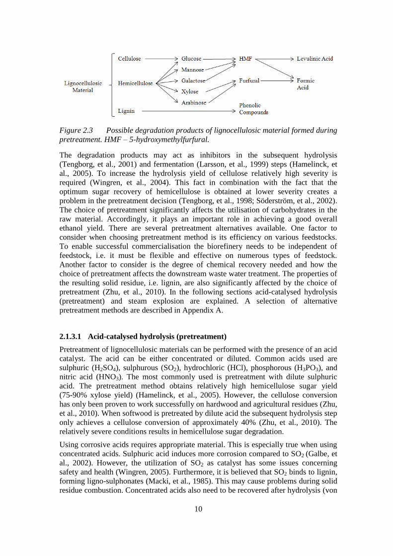
10

Figure 2.3 Possible degradation products of lignocellulosic material formed during

pretreatment. HMF – 5-hydroxymethylfurfural.

The degradation products may act as inhibitors in the subsequent hydrolysis

(Tengborg, et al., 2001) and fermentation (Larsson, et al., 1999) steps (Hamelinck, et

al., 2005). To increase the hydrolysis yield of cellulose relatively high severity is

required (Wingren, et al., 2004). This fact in combination with the fact that the

optimum sugar recovery of hemicellulose is obtained at lower severity creates a

problem in the pretreatment decision (Tengborg, et al., 1998; Söderström, et al., 2002).

The choice of pretreatment significantly affects the utilisation of carbohydrates in the

raw material. Accordingly, it plays an important role in achieving a good overall

ethanol yield. There are several pretreatment alternatives available. One factor to

consider when choosing pretreatment method is its efficiency on various feedstocks.

To enable successful commercialisation the biorefinery needs to be independent of

feedstock, i.e. it must be flexible and effective on numerous types of feedstock.

Another factor to consider is the degree of chemical recovery needed and how the

choice of pretreatment affects the downstream waste water treatment. The properties of

the resulting solid residue, i.e. lignin, are also significantly affected by the choice of

pretreatment (Zhu, et al., 2010). In the following sections acid-catalysed hydrolysis

(pretreatment) and steam explosion are explained. A selection of alternative

pretreatment methods are described in Appendix A.

2.1.3.1 Acid-catalysed hydrolysis (pretreatment)

Pretreatment of lignocellulosic materials can be performed with the presence of an acid

catalyst. The acid can be either concentrated or diluted. Common acids used are

sulphuric (H2SO4), sulphurous (SO2), hydrochloric (HCl), phosphorous (H3PO3), and

nitric acid (HNO3). The most commonly used is pretreatment with dilute sulphuric

acid. The pretreatment method obtains relatively high hemicellulose sugar yield

(75-90% xylose yield) (Hamelinck, et al., 2005). However, the cellulose conversion

has only been proven to work successfully on hardwood and agricultural residues (Zhu,

et al., 2010). When softwood is pretreated by dilute acid the subsequent hydrolysis step

only achieves a cellulose conversion of approximately 40% (Zhu, et al., 2010). The

relatively severe conditions results in hemicellulose sugar degradation.

Using corrosive acids requires appropriate material. This is especially true when using

concentrated acids. Sulphuric acid induces more corrosion compared to SO2 (Galbe, et

al., 2002). However, the utilization of SO2 as catalyst has some issues concerning

safety and health (Wingren, 2005). Furthermore, it is believed that SO2 binds to lignin,

forming ligno-sulphonates (Macki, et al., 1985). This may cause problems during solid

residue combustion. Concentrated acids also need to be recovered after hydrolysis (von

11

Sivers, et al., 1995). This is not required to the same extent when using dilute sulphuric

acid, due to the low purchase cost, to obtain an economically efficient process.

However, the hydrolysate pH must be neutralised prior the fermentation step in both

cases (Sun, et al., 2002). This results in the requirement of substantial amounts of

alkaline chemicals (e.g. lime) and a resulting solid residue (e.g. gypsum) requiring

deposition (Hamelinck, et al., 2005; Zhu, et al., 2010).

2.1.3.2 Steam explosion

One of the most investigated pretreatment methods for lignocellulosic feedstock is

steam explosion, also often referred to as steam pretreatment (Galbe, et al., 2002). The

size-reduced feedstock is treated with saturated high-pressure steam (6-28 bar,

160-260°C) (Sassner, 2007). The steam condenses and the wood structure “explodes”

with a sudden pressure release causing the condensed moisture to evaporate

(Carvalheiro, et al., 2008; Sun, et al., 2002). The method obtains a high yield of

solubilised hemicellulose, while lignin remains in the solid fraction (Carvalheiro, et al.,

2008). It can be performed with and without the addition of acid catalyst.

If no acid catalyst is added it is referred to as autohydrolysis. The absence of acid

catalyst results in a requirement of high severity in order to solubilise the

hemicellulose. As discussed earlier this may increase the formation of degradation

products, which results in a decreased overall hemicellulose sugar recovery and

possibly inhibition in the downstream hydrolysis and fermentation steps (Sassner,

2007).

Dilute-acid steam explosion is a combination of dilute-acid pretreatment and steam

explosion (Zhu, et al., 2010). It is considered to be the pretreatment method with the

highest potential, particularly for woody raw material (Galbe, et al., 2002). With the

addition of an acid catalyst the yield of hemicellulosic sugars is increased, furthermore

the cellulose hydrolysis in the following step is enhanced (Eklund, et al., 1995;

Wingren, et al., 2004). The increase of hemicellulose recovery is due to the reduced

severity needed resulting in a lower degree of hemicellulose degradation (Wingren, et

al., 2004; Eklund, et al., 1995; Sassner, 2007). The lower amount of inhibitors formed

may improve the cellulose hydrolysis yield (Sassner, 2007).

The size-reduced feedstock is first impregnated with dilute-acid and then treated with

steam. Dilute-acid steam pretreatment has similar drawbacks to dilute-acid

pretreatment, e.g. the need for pH-neutralisation resulting in solid residue requiring

deposition. The most extensively used acids are sulphuric acid and gaseous SO2.

Impregnation of SO2 and H2SO4 using spruce as feedstock results in the overall

fermentable sugar yield of approximately 66% and 65% respectively (Tengborg, et al.,

1998).

To increase the carbohydrate utilization in the raw material the pretreatment can be

divided into two separate steps, i.e. a two-step dilute acid steam pretreatment

(Söderström, et al., 2003; Nguyen, et al., 2000). This is favorable since the optimum

conditions for sugar recovery for hemicellulose and cellulose differs (Galbe, et al.,

2002; Stenberg, et al., 1998b). The first step is conducted at low severity solubilising

and hydrolysing the hemicellulose. In order to avoid formation of degradation

compounds the liquid and solid fraction are separated. 95% of the hemicellulosic

sugars can be recovered in the liquid fraction if the filter cake is washed (Sassner,

12

2007; Aden, et al., 2002). The liquid fraction bypasses the second pretreatment step

and also the hydrolysis step if operating the hydrolysis and fermentation steps

separately, see Section 2.1.5. The solid fraction is sent to the second pretreatment step

conducted at high severity making the cellulose more accessible for the subsequent

hydrolysis. The overall sugar yield increases from 65-66% to approximately 75-80%

dividing the pretreatment of spruce into two separate steps (Söderström, et al., 2003;

Nguyen, et al., 2000).

The most favorable conditions for maximising the sugar recovery using SO2 as acid

catalyst are an acid concentration of 3% and 190°C in the first step and 220°C in the

second step. Using H2SO4 the corresponding conditions are an acid concentration of

0.5% and 180°C in the first step and an acid concentration of 1% and 210°C in the

second pretreatment step. (Söderström, et al., 2005)

The advantages of a two-step dilute acid steam pretreatment are its enhanced

carbohydrate utilisation and high ethanol yield. If applying enzymatic hydrolysis, see

Section 2.1.4.1, the method also results in lower enzyme consumption (Galbe, et al.,

2002). On the other hand, the capital cost increases, requiring two separate

pretreatment reactors, and the pretreatment configuration results in comparatively

higher energy demand (Zhu, et al., 2010).

2.1.4 Hydrolysis

As mentioned in Section 2.1.3, the fermentable sugars in cellulose and hemicellulose

can be derived through hydrolysis. When handling lignocellulosic feedstock the

hydrolysis of hemicellulose is performed in the pretreatment step. The cellulose

hydrolysis occurs in the subsequent step referred to as the hydrolysis, or

saccharification, step. In cellulose hydrolysis, cellulose is broken down to its respective

sugar (i.e. glucose) according to reaction (2.1) (Hamelinck, et al., 2005):

(C6H10O5)n + nH2O → nC6H12O6 (2.1)

The hydrolysis yield can exceed 90% if the feedstock is pretreated (Hamelinck, et al.,

2005). The hydrolysis can be catalysed by acid (dilute or concentrated) or by enzymes.

Acid hydrolysis is conducted under similar circumstances as dilute- or concentrated

acid pretreatment respectively, see Section 2.1.3.1. The dilute acid hydrolysis process

is the first technology used for commercial ethanol production from cellulosic biomass

(Galbe, et al., 2002; Hamelinck, et al., 2005).

2.1.4.1 Enzymatic hydrolysis

The cellulose conversion to glucose by cellulase enzymes results in a very specific

reaction and is conducted at low severity (pH 4.0-5.0, temperature 45-50°C), thus

providing high yields and low sugar decomposition. The potential of the process is

very high, and it is considered as the most promising hydrolysis method in ethanol

production from lignocellulosic feedstock (Hamelinck, et al., 2005).

The conversion of glucose by enzymes from native cellulose is extremely slow, hence

pretreatment making the cellulose accessible to enzymes is essential. The enzymatic

hydrolysis efficiency decreases if biomass possesses characteristics as high

crystallinity, high cellulose polymerization degree, and high lignin content. Conversely

13

the efficiency is improved with large internal surface area. Cellulose hydrolysis by

enzymes is compatible with most pretreatment methods, except for pure mechanical

methods. Chips pretreated with steam explosion can reach conversions greater than

90% in the enzymatic hydrolysis step (Grous, et al., 1986).

Sugar degradation products formed in the preceding pretreatment may inhibit the

enzymatic hydrolysis process. Furthermore, cellulase enzymes are inhibited by

intermediate and end products formed during hydrolysis, i.e. cellobiose and glucose

(Hamelinck, et al., 2005; Sun, et al., 2002). This effect can be reduced if performing

the enzymatic hydrolysis at low dry matter content (Galbe, et al., 2002). Other

solutions to reduce the end-product inhibition are increasing the enzyme concentration

(e.g. through enzyme recovery and recycling), removing the end-product (e.g. through

ultrafiltration) or by allowing the hydrolysis and fermentation to occur in the same

reactor. The latter method is referred to as simultaneous saccharification and

fermentation (SSF), for more details see Section 2.1.5. (Hamelinck, et al., 2005; Sun, et

al., 2002)

Advantages of the enzymatic hydrolysis method are its high overall sugar yields and its

comparatively (to acid hydrolysis) lower equipment and maintenance costs. The

process is performed at low temperatures. The method does not require a subsequent

neutralisation step, accordingly no solid waste is (Hamelinck, et al., 2005).

2.1.5 Fermentation

Several microorganisms, e.g. bacteria, yeast, and fungi, have the ability to ferment

carbohydrates to ethanol. The most promising microorganisms in fermenting

lignocellulosics are the yeast Saccharomyces cerevisiae (ordinary baker’s yeast), and

the bacteria Zymomonas mobilis. The latter results in higher glucose to ethanol yield

(Galbe, et al., 2002). On the other hand, S. cerevisiae is tolerant to inhibitory

compounds and robust, i.e. very suitable for fermentation of lignocellulosics (Galbe, et

al., 2002; Olsson, et al., 1993). Moreover, it has the ability to ferment mannose and

after modification, also galactose (Galbe, et al., 2002). This is especially beneficial

when deriving sugars from softwood, see Table 2.1 in Section 2.1.1.1.

Lignocellulosic materials also consist of pentoses, i.e. xylose and arabinose. At

present, the conversion of pentoses to ethanol is relatively difficult. Microorganisms

can be adapted to increase the ability to ferment xylose and arabinose (Hamelinck, et

al., 2005; Galbe, et al., 2002). Progress has been achieved when S. cerevisiae,

Z. mobilis, and the bacteria Escherichia coli have been genetically engineered (Galbe,

et al., 2002; Hamelinck, et al., 2005).

The pentose and hexose sugar conversions to ethanol occur according to the following

reactions respectively (Hamelinck, et al., 2005):

3C5H10O5 → 5C2H5OH + 5CO2 (2.2)

C6H12O6 → 2C2H5OH + 2CO2 (2.3)

The enabling of pentose conversion would significantly increase the carbohydrate

utilisation of the raw material, and thus increase the ethanol efficiency and economy.

This would have particular impact for lignocellulosics with high proportion of

pentoses, i.e. agricultural residues and hardwood. The enabling of pentose fermentation

utilising softwood, would have comparatively less impact on the overall ethanol

14

efficiency. Nevertheless, it would not be without significance. Table 2.2 shows the

theoretical ethanol yield from hexoses and pentoses for spruce, salix, and corn stover

(with the feedstock composition presented in Table 2.1) respectively.

Table 2.2 Theoretical ethanol yield (kg ethanol/tonne dry feedstock) (Sassner, et

al., 2008)

Spruce Salix Corn stover

From hexoses 336 272 238

From pentoses 47 95 151

The cellulose hydrolysis and the hexose sugar fermentation to ethanol can be

conducted separately, in different reactors, or simultaneously, in the same reactor. The

first is referred to as separate hydrolysis and fermentation (SHF) and the latter to

simultaneous saccharification and fermentation (SSF). If also pentose fermentation is

occurring the corresponding processes are referred to as separate hydrolysis and

co-fermentation (SHCF) and simultaneous saccharification and co-fermentation

(SSCF). The main advantage to perform hydrolysis and fermentation separately is that

the two processes can be conducted under its respective optimal condition. Optimally,

the enzymatic hydrolysis is conducted at temperatures of 45-50°C, while fermentation

is carried out at 30°C (Galbe, et al., 2002). If hydrolysis and fermentation occurs

simultaneously the temperature is usually around 35°C (Galbe, et al., 2002). If thermo-

tolerant yeast can be developed the SSF performance is expected to be enhanced. As

mentioned in Section 2.1.4.1, the intermediate and end-products (i.e. cellobiose and

fermentable sugars respectively) inhibit the cellulases in the cellulose hydrolysis

process. This is the main drawback of SHF. Conversely, in the SSF configuration,

glucose and other fermentable sugars are immediately consumed by the yeast, i.e. end-

product inhibition is prevented. On the other hand, ethanol also inhibits cellulose

saccharification however not to the same extent. Another advantage with SSF is its

lower capital cost followed by the requirement of only one reactor. Conducting

hydrolysis and fermentation simultaneously (i.e. SSF) yeast is incorporated with the

solid lignin-rich residue, leading to problems in recovering and recycling of yeast.

(Galbe, et al., 2002)

2.1.6 Product purification

The fermentation broth consists of a wide variety of substances, both solids and

liquids. The ethanol dehydration to ethylene process requires an ethanol purity of

95 vol% (Kochar, et al., 1981). Ethanol is generally concentrated in two steps. In the

first step the solids and non-volatile substances are separated from the ethanol-water

mixture in a stripper. This separation unit is referred to as the beer column. The beer

column is followed by the rectification column, where ethanol purity approaches the

ethanol-water azeotrope (around 95 wt%). (Hamelinck, et al., 2005)

The energy consumption in the distillation step exponentially decreases with an

increasing ethanol concentration in the distillation feed (Galbe, et al., 2007; Wingren,

et al., 2008). As the distillation step is one of the most energy consuming process units

in the ethanol production, it has a major impact on the overall process energy demand.

Therefore, obtaining a high ethanol concentration after fermentation is of great

15

significance. Utilising lignocellulosic feedstock an ethanol concentration of

approximately 4 wt% is desired (Sassner, 2007).

The ethanol concentration can be further increased to 99.5-99.9 wt% (Cardona-Alzate,

et al., 2006; Hamelinck, et al., 2005). This is achieved through distillation performed

with an entrainer, drying with desiccants, using pervaporation, or membrane

techniques.

2.1.7 Evaporation

Beer column bottom product is sent to a solid-liquid separator. The liquid fraction is

sent to an evaporation unit to enable utilisation of the dissolved, non-volatile

substances as fuel. This implies that it is concentrated to sufficiently high dry matter

(DM) content at the expense of thermal energy. The resulting evaporation syrup is

mixed with the solid fraction (from solid-liquid separator) prior to combustion. The

resulting evaporate condensate is relatively free from non-volatile substances which

makes it suitable for water recycling, for more details see Section 2.1.8 (Larsson, et al.,

1997).

The evaporation process is relatively energy demanding. In order to reduce the energy

consumption it can be performed in multiple effects. It can be arranged as forward-

feed, counter-current, or as a combination of the two.

2.1.8 Recirculation of process streams

The ethanol production process from lignocellulosic material requires large quantities

of water in several process steps. In large-scale production internal recirculation of

process streams is necessary to decrease the fresh water consumption. Consequently

also the amount of wastewater is reduced. When recirculating process streams, energy

consumption is also decreased due to the reduced need for preheat of wash water. A

downside with recirculation is the accumulation of potential inhibitors in the hydrolysis

and fermentation (Larsson, et al., 1997; Stenberg, et al., 1998a). These compounds

originate from the raw material or are formed in the pretreatment step.

The selection of recirculation streams affects the flow through the various process

steps, hence also the energy consumption in the distillation and evaporation

(Alkasrawi, et al., 2002). The properties of the recycling stream affects the ethanol

yield, consequently it is of utmost importance to evaluate its respective suitability.

Non-volatile substances inhibit fermentation significantly, while hydrolysis is

moderately affected. Volatile substances do not inhibit the fermentation (Larsson, et

al., 1997). Therefore it is desirable to avoid recirculation of process streams containing

non-volatile substances. It has been shown that 60% of the fresh water can be replaced

by distillation stillage without negatively affecting the hydrolysis or fermentation. If

recirculating the stream before distillation the corresponding amount is 40%.

Recirculation of higher proportions will cause inhibition in the fermentation, however

not in the hydrolysis. The use of customised yeast or the investment of a detoxification

step could increase the recirculation proportion. (Alkasrawi, et al., 2002)

An effective alternative to reduce the inhibitory substances in the hydrolysis and

fermentation when recirculation process streams is evaporation, see Section 2.1.7. At

16

the expense of thermal energy possible inhibitors are removed. The concentrated

evaporation syrup, i.e. non-volatiles, can be utilised as fuel in a combined heat and

power (CHP) plant, see Section 2.1.9. Additionally the chemical (COD) and biological

(BOD7) oxygen demands of the distillation stillage are reduced by 90%, leading to a

cost reduction of the wastewater treatment of the evaporation condensate fraction that

is not recirculated. (Larsson, et al., 1997)

2.1.9 Combined Heat and Power (CHP) plant

The solid residue (i.e. mainly lignin) from beer column and concentrated evaporation

syrup are suitable as combustion fuel. Additionally, bark from the debarking unit can

used be as fuel. Available fuel can be utilised in a combined heat and power (CHP)

plant supplying steam and electricity to the process. Steam extraction possibilities are

available at several pressure levels.

2.1.10 Wastewater treatment (WWT)

The ethanol production process involves large water flows, as a result a water

purification step is necessary. It is mainly the resulting flash-vapor streams from the

pretreatment, the rectifier stillage, and possibly a fraction of the evaporation

condensate that require treatment. The wastewater treatment (WWT) is usually

performed in one anaerobic and one aerobic step. The feed streams are cooled to the

operating temperature of the digesters. In the anaerobic digestion 50% of the chemical

oxygen demand (COD) is consumed producing methane (Sassner, et al., 2008). The

biogas can be used as fuel in the steam generation unit. In the succeeding aerobic step

the greater part of the remaining COD is removed. The treated water can be considered

as clean. The wastewater treatment results in the formation of sludge, mainly in the

second aerobic step. This requires additional treatment. (Sassner, et al., 2008)

2.2 Stand-alone ethanol dehydration to ethylene

production

2.2.1 Stand-alone ethanol dehydration to ethylene production

configuration

In 2010 Braskem started a full-scale ethanol dehydration plant in Brazil (Braskem,

2010). The ethanol dehydration process basically consists of a reactor and several

purification steps. The Braskem patent mainly focuses on the reactor, which is

adiabatic. The reactor feed is diluted with steam to a large extent. The patent reveals

limited information and the heat exchanger network is specified. Halcon SD developed

a process in the 1960’s (Kochar, et al., 1981) that is used by the process plant supplier

Chematur International AB (Chematur AB). Research has been performed and

published on the process, i.e. some process data is available (Chematur AB; Kochar, et

al., 1981)

Figure 2.4 illustrates an overview of assumed stand-alone ethanol dehydration to

ethylene production configuration investigated in the study. The assumed process

configuration is based on a literature review. The assumed process configuration is

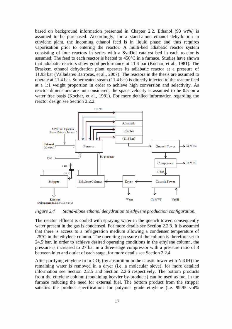
17

based on background information presented in Chapter 2.2. Ethanol (93 wt%) is

assumed to be purchased. Accordingly, for a stand-alone ethanol dehydration to

ethylene plant, the incoming ethanol feed is in liquid phase and thus requires

vaporisation prior to entering the reactor. A multi-bed adiabatic reactor system

consisting of four reactors in series with a SynDol catalyst bed in each reactor is

assumed. The feed to each reactor is heated to 450°C in a furnace. Studies have shown

that adiabatic reactors show good performance at 11.4 bar (Kochar, et al., 1981). The

Braskem ethanol dehydration plant operates its adiabatic reactor at a pressure of

11.93 bar (Valladares Barrocas, et al., 2007). The reactors in the thesis are assumed to

operate at 11.4 bar. Superheated steam (11.4 bar) is directly injected to the reactor feed

at a 1:1 weight proportion in order to achieve high conversion and selectivity. As

reactor dimensions are not considered, the space velocity is assumed to be 0.5 on a

water free basis (Kochar, et al., 1981). For more detailed information regarding the

reactor design see Section 2.2.2.

Figure 2.4 Stand-alone ethanol dehydration to ethylene production configuration.

The reactor effluent is cooled with spraying water in the quench tower, consequently

water present in the gas is condensed. For more details see Section 2.2.3. It is assumed

that there is access to a refrigeration medium allowing a condenser temperature of

-25°C in the ethylene column. The operating pressure of the column is therefore set to

24.5 bar. In order to achieve desired operating conditions in the ethylene column, the

pressure is increased to 27 bar in a three-stage compressor with a pressure ratio of 3

between inlet and outlet of each stage, for more details see Section 2.2.4.

After purifying ethylene from CO2 (by absorption in the caustic tower with NaOH) the

remaining water is removed in a dryer (i.e. a molecular sieve), for more detailed

information see Section 2.2.5 and Section 2.2.6 respectively. The bottom products

from the ethylene column (containing heavier by-products) can be used as fuel in the

furnace reducing the need for external fuel. The bottom product from the stripper

satisfies the product specifications for polymer grade ethylene (i.e. 99.95 vol%

18

ethylene), see Table 2.3. For further information about the ethylene column and

stripper see Section 2.2.7.

2.2.2 Reactor

The reactor is the most important unit in the ethanol dehydration to ethylene process. It

is where the conversion of ethanol to ethylene occurs.

2.2.2.1 Catalytic reaction

Ethylene from ethanol dehydration is a catalytic endothermic reaction. Chematur uses

a SynDol, i.e. aluminum-oxide, catalyst developed by Halcon SD (Kochar, et al., 1981;

Chematur AB). Ethylene (C2H4) formation is predominant in temperature regions of

320°C – 500°C, while in temperature regions of 150°C – 300°C the formation of

diethyleter (C4H10O) is predominant, see reactions (2.4) and (2.5) respectively

(Morschbaker, 2009; Kochar, et al., 1981; Valladares Barrocas, et al., 1980).

Consequently, the operating conditions in the reactor are of utmost importance to

achieve high selectivity towards ethylene.

C2H5OH → C2H4 + H2O (2.4)

2C2H5OH → C4H10O + H2O (2.5)

Ethylene can also be formed with diethyleter as an intermediate, see reaction (2.6).

This makes the contact time with the catalyst an important parameter in order to

achieve the desired product, i.e. ethylene (Valladares Barrocas, et al., 1980).

2C2H5OH → C4H10O + H2O

→ C2H4 + H2O (2.6)

At temperatures above 500°C the formation of acetaldehyde, see reaction (2.7),

increases (Kochar, et al., 1981). As a result the ethylene selectivity is reduced.

C2H5OH → C2H4O + H2 (2.7)

Additional reactions occurring during ethanol dehydration are the formation of by-

products, such as propene (C3H6), buthylene (C4H8), ethane (C2H6), carbon monoxide

(CO) and carbon dioxide (CO2). High ethanol conversion (up to 99.9%) and high

selectivity towards ethylene (94.5-99%) can be achieved operating at the right reactor

conditions (Valladares Barrocas, et al., 1980; Kochar, et al., 1981).

2.2.2.2 Adiabatic versus isothermal reactors

As mentioned in Section 2.2.2.1, the ethanol dehydration reaction is endothermic and

the product formation is highly temperature dependent. Therefore the operating

temperature is required to be kept in a certain range in order to govern the selectivity

towards ethylene. This can be achieved with either adiabatic or isothermal reactors.

Isothermal reactors operate with a circulating heating fluid outside the reactor

supplying heat and maintaining the temperature in the reactor. Commercial heating

fluids have a maximum working temperature of approximately 370°C, due to thermal

decomposition (Kochar, et al., 1981). As a concequence the reactor is limited to

19

relatively low operating temperatures, resulting in reduced ethanol conversion and

ethylene selectivity (Morschbaker, 2009; Kochar, et al., 1981). To provide sufficient

heat to the reactor, i.e. maintain the temperature, the area is increased by introducing a

tube-package. The large number of tubes will increase the capital cost for the reactor

(Valladares Barrocas, et al., 1980).

Operating with adiabatic reactors, the heating fluid outside the tubes is avoided. This

will enable operating temperatures above 370°C. Thus the reactor inlet temperature can

reach temperature regions of 450°C – 500°C (Kochar, et al., 1981; Morschbaker,

2009). The reactor can consist of one reactor or several in series or in parallel. The

process used by Chematur International AB uses four tubular adiabatic reactors

connected in series. Since the reaction is endothermic the effluent from each reactor

requires reheating before entering the subsequent reactor. If the temperature is kept

within an appropriate range, high ethanol conversion and high ethylene selectivity will

be obtained. Additionally, higher selectivity towards ethylene results in lower

production of by-products which require removal downstream in the process in several

purification steps. The capital cost for adiabatic reactors is comparatively lower than

for isothermal reactors (Kochar, et al., 1981).

2.2.2.3 Reactors operating conditions

The operating conditions of the reactor have a significant effect on obtained conversion

and selectivity. The effects of changes of temperature, pressure, steam dilution of feed,

and space velocity have been investigated (Kochar, et al., 1981). As already mentioned

in Section 2.2.2.1, operating temperature has a significant effect on the ethylene yield.

Adequate operating temperature (isothermal reactor) and inlet temperature (adiabatic

reactor) to maintain high conversion and selectivity in/throughout the reactor is

important. Ethanol conversion and ethylene selectivity decreases with increasing

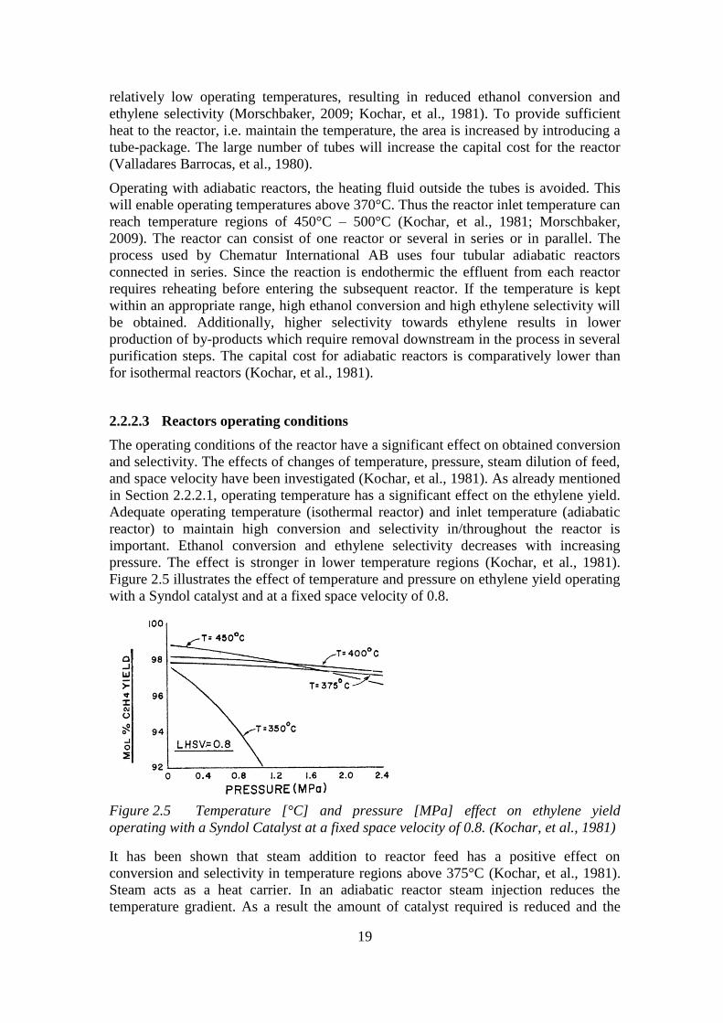
pressure. The effect is stronger in lower temperature regions (Kochar, et al., 1981).

Figure 2.5 illustrates the effect of temperature and pressure on ethylene yield operating

with a Syndol catalyst and at a fixed space velocity of 0.8.

Figure 2.5 Temperature [°C] and pressure [MPa] effect on ethylene yield

operating with a Syndol Catalyst at a fixed space velocity of 0.8. (Kochar, et al., 1981)

It has been shown that steam addition to reactor feed has a positive effect on

conversion and selectivity in temperature regions above 375°C (Kochar, et al., 1981).

Steam acts as a heat carrier. In an adiabatic reactor steam injection reduces the

temperature gradient. As a result the amount of catalyst required is reduced and the

20

formation of by-products (such as diethyleter) is reduced. Additionally a lower

frequency of catalyst regeneration is required due to less coke formation and the

catalyst lifetime increases (Morschbaker, 2009; Valladares Barrocas, et al., 1980).

However, the addition of steam results in higher heating demand if operating with

several adiabatic reactors (in e.g. series) when reheating the effluent of the reactors.

The contact time with the catalyst has a significant effect on the selectivity towards

ethylene. The selectivity towards ethylene is decreased with increasing space velocity,

see reaction (2.6).

2.2.2.4 Furnace

A furnace provides sufficient heat to the reactor(s) to enable desired operating

temperature.

2.2.3 Quench tower

In the quench tower, water present in the reactor effluent stream is condensed by

cooling the entering gas with spray water from the top of the tower. The liquid, in the

bottom of the tower contains condensed water, impurities, and unconverted ethanol

(Winter, et al., 1976). A fraction of the bottom product is cooled and recirculated back

as spray-water, while the remainder is sent to the wastewater treatment.

2.2.4 Compressor

The gas stream leaving the quench tower mainly consists of ethylene. In order to

enable sufficient pressure through downstream units the gas is compressed in a

multi-stage compressor. Between each compressor stage an intercooler and a knock-

out drum is placed, removing some of the remaining water. Literature states outlet

pressures from the last compressor between 20-29 bar (Kochar, et al., 1981; Huang,

2010). The outlet pressure is set to obtain desirable operating temperature in the

downstream ethylene column condenser.

2.2.5 Caustic tower

In the caustic tower CO2 is absorbed by washing the gas with sodium hydroxide

(NaOH) in a packed column. The final ethylene product needs to fulfill the product

specification of maximum 10 vol-ppm CO2 in order to enable polymerisation (Kochar,

et al., 1981). On top of the caustic tower a water wash is placed spraying water on the

gas. As a result the sodium hydroxide is washed out.

2.2.6 Dryer

The remaining water is removed in a dryer. The incoming gas is first cooled prior

entering a molecular sieve. The gas leaving the dryer contains zero or close to zero

moles of water.

21

2.2.7 Ethylene column and stripper

After the dryer, heavier impurities are removed in a cryogenic distillation column. The

ethylene column, also referred to as the C2-splitter, essentially separates ethane from

ethylene. The light key component is ethylene and the heavy key component is ethane.

The operating temperature for the column is restricted by available cooling medium.

The bottom product consists of heavier carbohydrates, ethanol, diethyleter, and

acetaldehyde, which e.g. can be used as fuel. The condenser serves as a joint condenser

for both ethylene column and stripper (Chematur AB). In the stripper carbon monoxide

(CO), methane (CH4), and hydrogen (H2) are separated from ethylene. To minimise

ethylene losses the top product of the stripper is sent to the joint condenser. In the

condenser the light by-products separated in the stripper is vented to air while the

condensed phase (containing mainly ethylene) is recirculated to ethylene column and

stripper.

The final ethylene product has to meet certain purity specifications prior to

polymerisation, i.e. it must be of polymer grade (which means having a purity of

99.85 – 99.95 vol% ethylene (Kochar, et al., 1981). Acceptable impurity levels are

shown in Table 2.3. This requirement must be achieved in order to obtain desirable

product qualities and also because the PE-catalyst is oxygen sensitive.

Table 2.3 Polymer grade ethylene (Kochar, et al., 1981).

Component Composition

Ethylene (vol%) 99.95

Carbon Monoxide (vol ppm) 5

Carbon Dioxide (vol ppm) 10

Ethane (vol%) 0.05

2.3 Biorefinery - Ethylene production from lignocellulosic

feedstock

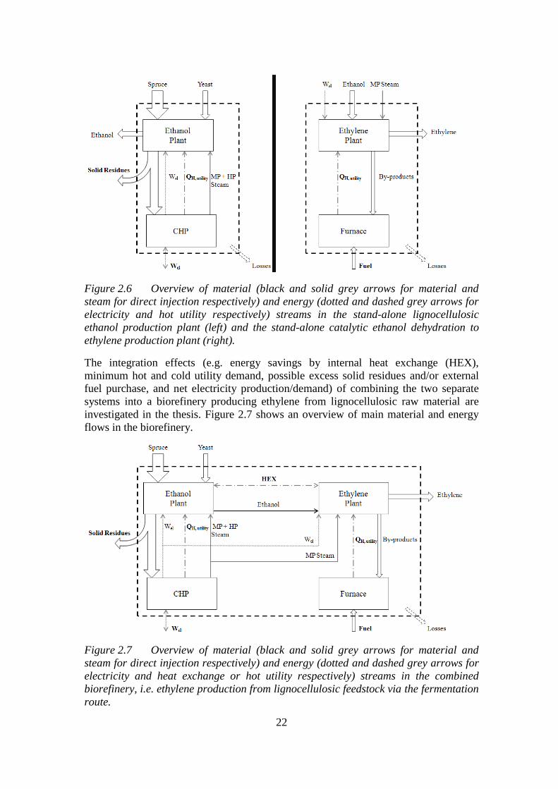
The heat integration potential of a stand-alone lignocellulosic ethanol production via

fermentation route plant and a stand-alone ethylene production through catalytic

dehydration of ethanol plant is investigated in the thesis. Figure 2.6 shows an overview

of the main material and energy flows in the two separate systems.

22

Figure 2.6 Overview of material (black and solid grey arrows for material and

steam for direct injection respectively) and energy (dotted and dashed grey arrows for

electricity and hot utility respectively) streams in the stand-alone lignocellulosic

ethanol production plant (left) and the stand-alone catalytic ethanol dehydration to

ethylene production plant (right).

The integration effects (e.g. energy savings by internal heat exchange (HEX),

minimum hot and cold utility demand, possible excess solid residues and/or external

fuel purchase, and net electricity production/demand) of combining the two separate

systems into a biorefinery producing ethylene from lignocellulosic raw material are

investigated in the thesis. Figure 2.7 shows an overview of main material and energy

flows in the biorefinery.



electricity and heat exchange or hot utility respectively) streams in the combined

biorefinery, i.e. ethylene production from lignocellulosic feedstock via the fermentation

route.

23

2.4 Chemical cluster

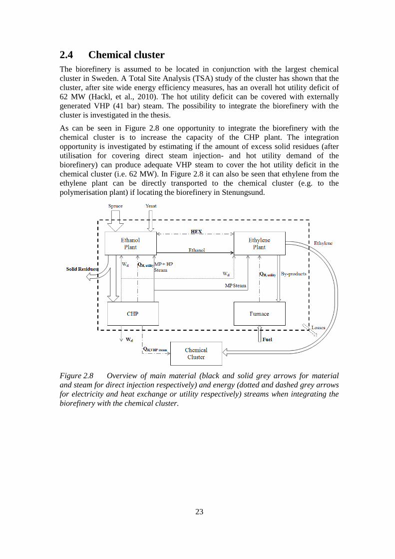
The biorefinery is assumed to be located in conjunction with the largest chemical

cluster in Sweden. A Total Site Analysis (TSA) study of the cluster has shown that the

cluster, after site wide energy efficiency measures, has an overall hot utility deficit of

62 MW (Hackl, et al., 2010). The hot utility deficit can be covered with externally

generated VHP (41 bar) steam. The possibility to integrate the biorefinery with the

cluster is investigated in the thesis.

As can be seen in Figure 2.8 one opportunity to integrate the biorefinery with the

chemical cluster is to increase the capacity of the CHP plant. The integration

opportunity is investigated by estimating if the amount of excess solid residues (after

utilisation for covering direct steam injection- and hot utility demand of the

biorefinery) can produce adequate VHP steam to cover the hot utility deficit in the

chemical cluster (i.e. 62 MW). In Figure 2.8 it can also be seen that ethylene from the

ethylene plant can be directly transported to the chemical cluster (e.g. to the

polymerisation plant) if locating the biorefinery in Stenungsund.

Figure 2.8 Overview of main material (black and solid grey arrows for material

and steam for direct injection respectively) and energy (dotted and dashed grey arrows

for electricity and heat exchange or utility respectively) streams when integrating the

biorefinery with the chemical cluster.

25

3 Methodology

A literature study was conducted in order to establish a simulation model for a stand-

alone ethanol from lignocellulosic feedstock (via fermentation route) production plant

and a stand-alone ethanol dehydration to ethylene plant. The study of the two stand-

alone processes is based on the production assumption of 200 000 tonnes ethylene

annually. Material- and energy balances for the two separate processes are solved in

the commercial flowsheeting software Aspen Plus from Aspen Technology. From

simulation results obtained a process integration study is conducted based on pinch

analysis. The heat integration potential of a stand-alone ethanol production plant and a

stand-alone ethylene production plant are investigated. The energy saving potential of

integrating the two stand-alone processes is investigated in a background/foreground

analysis. Furthermore the effects (e.g. minimum hot and cold utility demand, possible

excess solid residues and/or external fuel purchase, and net electricity

production/demand) of integrating the two processes into a biorefinery producing

ethylene from lignocellulosic feedstock are also investigated. Several biorefinery

configurations are investigated; e.g. the integration opportunity for the biorefinery (i.e.

ethylene production from lignocellulosic feedstock) to deliver VHP steam, by

increasing the CHP plant capacity, to the chemical cluster.

3.1 Stand-alone lignocellulosic ethanol production

simulations in Aspen Plus

The NRTL property method with Henry components is used in the ethanol production

simulations recommended by guidelines in Aspen Plus. The NRTL property method is

recommended for e.g. liquid phase reactions and azeotropic alcohol separation. The

property method uses Henry’s law for vapor-liquid binary interactions.

3.1.1 Components

The composition for spruce in Table 2.1 is used as feedstock composition in the

simulations, see Section 2.1.1.1. Some of the materials included in the process are

water insoluble and are only present in solid state and do not participate in liquid-liquid

or vapor-liquid equilibriums. To enable handling of solid material in the system two

substreams are used: one vapor-liquid stream (MIXED) and one solid stream

(CISOLID).

Some of the materials involved in the ethanol production do not exist in the

conventional databanks in Aspen Plus. In order to obtain the required physical

properties of the materials to enable mass- and energy balance calculations data are

taken from a NREL database for biofuel component (Wooley, et al., 1996). Examples

of materials including in the legacy databank are cellulose, xylan, and lignin. HMF and

soluble lignin are not included in the database and are added as user defined

components. Examples of required specified data are chemical formula, boiling point,

and coefficients to the Extended Antoine vapor pressure equation and the Ideal gas

heat capacity equation. For more details see Appendix B.

26

The hexosans glucan, mannan, and galactan are assumed to have the same properties as

cellulose (Wooley, et al., 1996; Aden, et al., 2002). The pentosans xylan and arabinan

are assumed to have the same properties, hence arabinan is modeled as xylan (Wooley,

et al., 1996; Aden, et al., 2002). Wood also consists of extractives. The extractives are

assumed to have the composition of “Others” in Table 2.1 (see Section 2.1.1.1) and are

modeled as one volatile (α-pinene) and one non-volatile (oleic acid) component

(Sassner, 2007). Ash is assumed to consist of CaO (Sassner, 2007). Initially all wood

components, with the exception of extractives, are in solid state. The moisture content

of wood is assumed to be 50% (Wingren, et al., 2003).

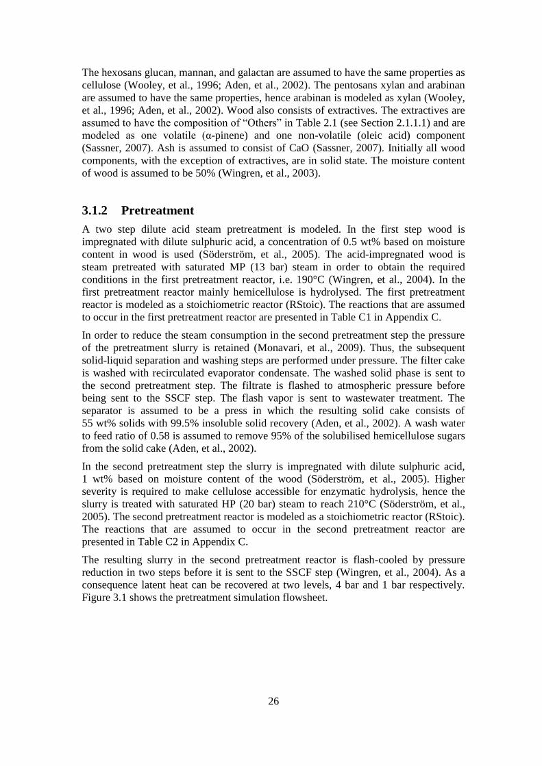
3.1.2 Pretreatment

A two step dilute acid steam pretreatment is modeled. In the first step wood is

impregnated with dilute sulphuric acid, a concentration of 0.5 wt% based on moisture

content in wood is used (Söderström, et al., 2005). The acid-impregnated wood is

steam pretreated with saturated MP (13 bar) steam in order to obtain the required

conditions in the first pretreatment reactor, i.e. 190°C (Wingren, et al., 2004). In the

first pretreatment reactor mainly hemicellulose is hydrolysed. The first pretreatment

reactor is modeled as a stoichiometric reactor (RStoic). The reactions that are assumed

to occur in the first pretreatment reactor are presented in Table C1 in Appendix C.

In order to reduce the steam consumption in the second pretreatment step the pressure

of the pretreatment slurry is retained (Monavari, et al., 2009). Thus, the subsequent

solid-liquid separation and washing steps are performed under pressure. The filter cake

is washed with recirculated evaporator condensate. The washed solid phase is sent to

the second pretreatment step. The filtrate is flashed to atmospheric pressure before

being sent to the SSCF step. The flash vapor is sent to wastewater treatment. The

separator is assumed to be a press in which the resulting solid cake consists of

55 wt% solids with 99.5% insoluble solid recovery (Aden, et al., 2002). A wash water

to feed ratio of 0.58 is assumed to remove 95% of the solubilised hemicellulose sugars

from the solid cake (Aden, et al., 2002).

In the second pretreatment step the slurry is impregnated with dilute sulphuric acid,

1 wt% based on moisture content of the wood (Söderström, et al., 2005). Higher

severity is required to make cellulose accessible for enzymatic hydrolysis, hence the

slurry is treated with saturated HP (20 bar) steam to reach 210°C (Söderström, et al.,

2005). The second pretreatment reactor is modeled as a stoichiometric reactor (RStoic).

The reactions that are assumed to occur in the second pretreatment reactor are

presented in Table C2 in Appendix C.

The resulting slurry in the second pretreatment reactor is flash-cooled by pressure

reduction in two steps before it is sent to the SSCF step (Wingren, et al., 2004). As a

consequence latent heat can be recovered at two levels, 4 bar and 1 bar respectively.

Figure 3.1 shows the pretreatment simulation flowsheet.

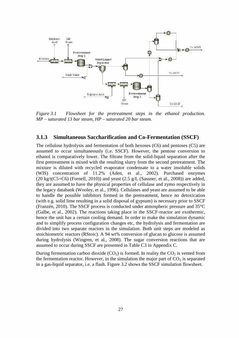
27

Figure 3.1 Flowsheet for the pretreatment steps in the ethanol production.

MP – saturated 13 bar steam, HP – saturated 20 bar steam.

3.1.3 Simultaneous Saccharification and Co-Fermentation (SSCF)

The cellulose hydrolysis and fermentation of both hexoses (C6) and pentoses (C5) are

assumed to occur simultaneously (i.e. SSCF). However, the pentose conversion to

ethanol is comparatively lower. The filtrate from the solid-liquid separation after the

first pretreatment is mixed with the resulting slurry from the second pretreatment. The

mixture is diluted with recycled evaporator condensate to a water insoluble solids

(WIS) concentration of 11.2% (Aden, et al., 2002). Purchased enzymes

(20 kg/t(C5+C6) (Fornell, 2010)) and yeast (2.5 g/L (Sassner, et al., 2008)) are added,

they are assumed to have the physical properties of cellulase and zymo respectively in

the legacy databank (Wooley, et al., 1996). Cellulases and yeast are assumed to be able

to handle the possible inhibitors formed in the pretreatment, hence no detoxication

(with e.g. solid lime resulting in a solid disposal of gypsum) is necessary prior to SSCF

(Franzén, 2010). The SSCF process is conducted under atmospheric pressure and 35°C

(Galbe, et al., 2002). The reactions taking place in the SSCF-reactor are exothermic,

hence the unit has a certain cooling demand. In order to make the simulation dynamic

and to simplify process configuration changes etc, the hydrolysis and fermentation are

divided into two separate reactors in the simulation. Both unit steps are modeled as

stoichiometric reactors (RStoic). A 94 wt% conversion of glucan to glucose is assumed

during hydrolysis (Wingren, et al., 2008). The sugar conversion reactions that are

assumed to occur during SSCF are presented in Table C3 in Appendix C.

During fermentation carbon dioxide (CO2) is formed. In reality the CO2 is vented from

the fermentation reactor. However, in the simulation the major part of CO2 is separated

in a gas-liquid separator, i.e. a flash. Figure 3.2 shows the SSCF simulation flowsheet.

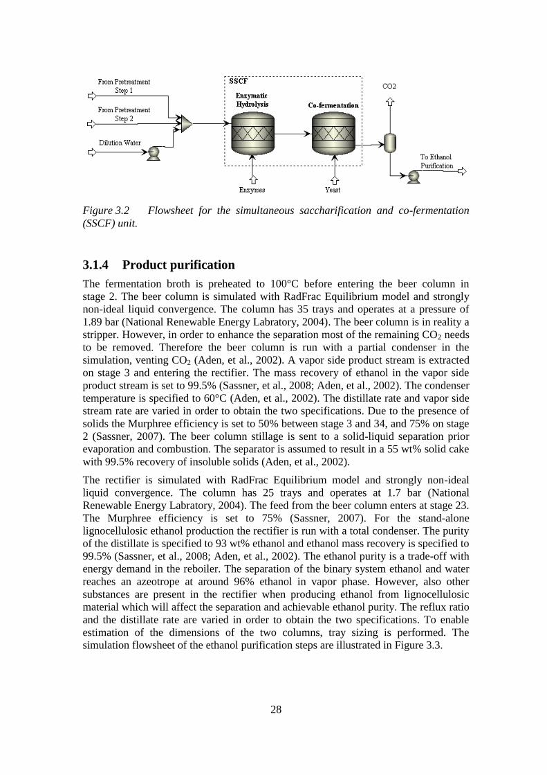
28

Figure 3.2 Flowsheet for the simultaneous saccharification and co-fermentation

(SSCF) unit.

3.1.4 Product purification

The fermentation broth is preheated to 100°C before entering the beer column in

stage 2. The beer column is simulated with RadFrac Equilibrium model and strongly

non-ideal liquid convergence. The column has 35 trays and operates at a pressure of

1.89 bar (National Renewable Energy Labratory, 2004). The beer column is in reality a

stripper. However, in order to enhance the separation most of the remaining CO2 needs

to be removed. Therefore the beer column is run with a partial condenser in the

simulation, venting CO2 (Aden, et al., 2002). A vapor side product stream is extracted

on stage 3 and entering the rectifier. The mass recovery of ethanol in the vapor side

product stream is set to 99.5% (Sassner, et al., 2008; Aden, et al., 2002). The condenser

temperature is specified to 60°C (Aden, et al., 2002). The distillate rate and vapor side

stream rate are varied in order to obtain the two specifications. Due to the presence of

solids the Murphree efficiency is set to 50% between stage 3 and 34, and 75% on stage

2 (Sassner, 2007). The beer column stillage is sent to a solid-liquid separation prior

evaporation and combustion. The separator is assumed to result in a 55 wt% solid cake

with 99.5% recovery of insoluble solids (Aden, et al., 2002).

The rectifier is simulated with RadFrac Equilibrium model and strongly non-ideal

liquid convergence. The column has 25 trays and operates at 1.7 bar (National

Renewable Energy Labratory, 2004). The feed from the beer column enters at stage 23.

The Murphree efficiency is set to 75% (Sassner, 2007). For the stand-alone

lignocellulosic ethanol production the rectifier is run with a total condenser. The purity

of the distillate is specified to 93 wt% ethanol and ethanol mass recovery is specified to

99.5% (Sassner, et al., 2008; Aden, et al., 2002). The ethanol purity is a trade-off with

energy demand in the reboiler. The separation of the binary system ethanol and water

reaches an azeotrope at around 96% ethanol in vapor phase. However, also other

substances are present in the rectifier when producing ethanol from lignocellulosic

material which will affect the separation and achievable ethanol purity. The reflux ratio

and the distillate rate are varied in order to obtain the two specifications. To enable

estimation of the dimensions of the two columns, tray sizing is performed. The

simulation flowsheet of the ethanol purification steps are illustrated in Figure 3.3.

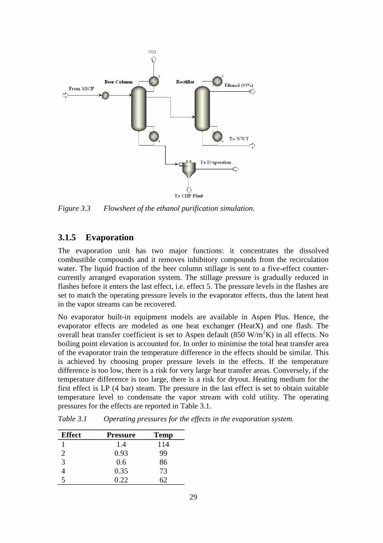
29

Figure 3.3 Flowsheet of the ethanol purification simulation.

3.1.5 Evaporation

The evaporation unit has two major functions: it concentrates the dissolved

combustible compounds and it removes inhibitory compounds from the recirculation

water. The liquid fraction of the beer column stillage is sent to a five-effect counter-

currently arranged evaporation system. The stillage pressure is gradually reduced in

flashes before it enters the last effect, i.e. effect 5. The pressure levels in the flashes are

set to match the operating pressure levels in the evaporator effects, thus the latent heat

in the vapor streams can be recovered.

No evaporator built-in equipment models are available in Aspen Plus. Hence, the

evaporator effects are modeled as one heat exchanger (HeatX) and one flash. The

overall heat transfer coefficient is set to Aspen default (850 W/m2K) in all effects. No

boiling point elevation is accounted for. In order to minimise the total heat transfer area

of the evaporator train the temperature difference in the effects should be similar. This

is achieved by choosing proper pressure levels in the effects. If the temperature

difference is too low, there is a risk for very large heat transfer areas. Conversely, if the

temperature difference is too large, there is a risk for dryout. Heating medium for the

first effect is LP (4 bar) steam. The pressure in the last effect is set to obtain suitable

temperature level to condensate the vapor stream with cold utility. The operating

pressures for the effects are reported in Table 3.1.

Table 3.1 Operating pressures for the effects in the evaporation system.

Effect Pressure Temp

1 1.4 114

2 0.93 99

3 0.6 86

4 0.35 73

5 0.22 62

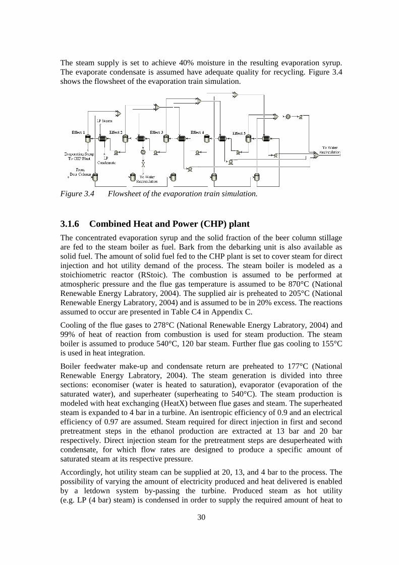
30

The steam supply is set to achieve 40% moisture in the resulting evaporation syrup.

The evaporate condensate is assumed have adequate quality for recycling. Figure 3.4

shows the flowsheet of the evaporation train simulation.

Figure 3.4 Flowsheet of the evaporation train simulation.

3.1.6 Combined Heat and Power (CHP) plant

The concentrated evaporation syrup and the solid fraction of the beer column stillage

are fed to the steam boiler as fuel. Bark from the debarking unit is also available as

solid fuel. The amount of solid fuel fed to the CHP plant is set to cover steam for direct

injection and hot utility demand of the process. The steam boiler is modeled as a

stoichiometric reactor (RStoic). The combustion is assumed to be performed at

atmospheric pressure and the flue gas temperature is assumed to be 870°C (National

Renewable Energy Labratory, 2004). The supplied air is preheated to 205°C (National

Renewable Energy Labratory, 2004) and is assumed to be in 20% excess. The reactions

assumed to occur are presented in Table C4 in Appendix C.

Cooling of the flue gases to 278°C (National Renewable Energy Labratory, 2004) and

99% of heat of reaction from combustion is used for steam production. The steam

boiler is assumed to produce 540°C, 120 bar steam. Further flue gas cooling to 155°C

is used in heat integration.

Boiler feedwater make-up and condensate return are preheated to 177°C (National

Renewable Energy Labratory, 2004). The steam generation is divided into three

sections: economiser (water is heated to saturation), evaporator (evaporation of the

saturated water), and superheater (superheating to 540°C). The steam production is

modeled with heat exchanging (HeatX) between flue gases and steam. The superheated

steam is expanded to 4 bar in a turbine. An isentropic efficiency of 0.9 and an electrical

efficiency of 0.97 are assumed. Steam required for direct injection in first and second

pretreatment steps in the ethanol production are extracted at 13 bar and 20 bar

respectively. Direct injection steam for the pretreatment steps are desuperheated with

condensate, for which flow rates are designed to produce a specific amount of

saturated steam at its respective pressure.

Accordingly, hot utility steam can be supplied at 20, 13, and 4 bar to the process. The

possibility of varying the amount of electricity produced and heat delivered is enabled

by a letdown system by-passing the turbine. Produced steam as hot utility

(e.g. LP (4 bar) steam) is condensed in order to supply the required amount of heat to

31

the process. The condensate is returned to the steam boiler. The feedwater make-up

flow rate is designed to produce the maximum amount of steam with the heat available

from the steam boiler. That is, the feedwater compensates for the extracted direct

injection steam in the turbine and for the condensate required for desuperheating.

Figure 3.5 illustrates the flowsheet of the Combined Heat and Power (CHP) plant

simulation.

Figure 3.5 Flowsheet of the Combined Heat and Power (CHP) plant simulation.

3.2 Stand-alone ethanol dehydration to ethylene

production simulations in Aspen Plus

The Peng-Robinson property method is used in the ethanol dehydration simulations

recommended by guidelines in Aspen Plus. The Peng-Robinson property method is

recommended when handling light hydrocarbons in e.g. an ethylene plant. The

separation units in the ethanol dehydration process are considered similar to those in a

traditional ethylene production process with naphtha as feedstock. Therefore the Peng-

Robinson property method is chosen for all non-electrolyte systems in the process.

3.2.1 Components

The physical properties for relevant components are acquired from the conventional

database in Aspen Plus. No solid substances are present in the ethanol dehydration

process, thus no solid substream (CISOLID) is used. In the simulation only a mixed

substream (MIXED), handling liquid and vapor, is present.

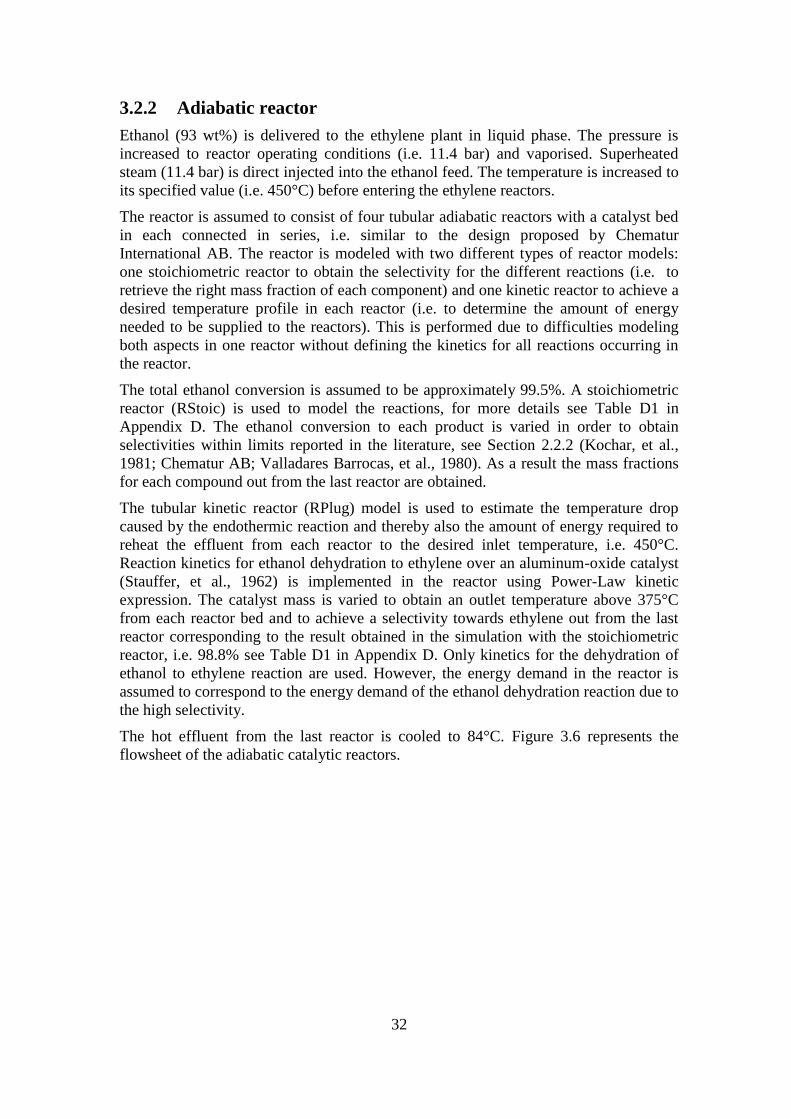
32

3.2.2 Adiabatic reactor

Ethanol (93 wt%) is delivered to the ethylene plant in liquid phase. The pressure is

increased to reactor operating conditions (i.e. 11.4 bar) and vaporised. Superheated

steam (11.4 bar) is direct injected into the ethanol feed. The temperature is increased to

its specified value (i.e. 450°C) before entering the ethylene reactors.

The reactor is assumed to consist of four tubular adiabatic reactors with a catalyst bed

in each connected in series, i.e. similar to the design proposed by Chematur

International AB. The reactor is modeled with two different types of reactor models:

one stoichiometric reactor to obtain the selectivity for the different reactions (i.e. to

retrieve the right mass fraction of each component) and one kinetic reactor to achieve a

desired temperature profile in each reactor (i.e. to determine the amount of energy

needed to be supplied to the reactors). This is performed due to difficulties modeling

both aspects in one reactor without defining the kinetics for all reactions occurring in

the reactor.

The total ethanol conversion is assumed to be approximately 99.5%. A stoichiometric

reactor (RStoic) is used to model the reactions, for more details see Table D1 in

Appendix D. The ethanol conversion to each product is varied in order to obtain

selectivities within limits reported in the literature, see Section 2.2.2 (Kochar, et al.,

1981; Chematur AB; Valladares Barrocas, et al., 1980). As a result the mass fractions

for each compound out from the last reactor are obtained.

The tubular kinetic reactor (RPlug) model is used to estimate the temperature drop

caused by the endothermic reaction and thereby also the amount of energy required to

reheat the effluent from each reactor to the desired inlet temperature, i.e. 450°C.

Reaction kinetics for ethanol dehydration to ethylene over an aluminum-oxide catalyst

(Stauffer, et al., 1962) is implemented in the reactor using Power-Law kinetic

expression. The catalyst mass is varied to obtain an outlet temperature above 375°C

from each reactor bed and to achieve a selectivity towards ethylene out from the last

reactor corresponding to the result obtained in the simulation with the stoichiometric

reactor, i.e. 98.8% see Table D1 in Appendix D. Only kinetics for the dehydration of

ethanol to ethylene reaction are used. However, the energy demand in the reactor is

assumed to correspond to the energy demand of the ethanol dehydration reaction due to

the high selectivity.

The hot effluent from the last reactor is cooled to 84°C. Figure 3.6 represents the

flowsheet of the adiabatic catalytic reactors.

33

Figure 3.6 Flowsheet of ethanol dehydration to ethylene reactor unit.

3.2.3 Quench tower

The quench tower is simulated with RadFrac equilibrium model. The tower is assumed

to have 14 stages and the operating pressure is set to atmospheric pressure. At the top

of the tower water (20°C) is sprayed, causing water in the gas to condense. A fraction

of the bottom product is cooled to 20°C and recirculated as spray-water. The water

recirculation mass flow is designed to obtain a mole fraction of ethylene in the top

product of 0.91. The quench tower flowsheet is illustrated in Figure 3.7.

Figure 3.7 Flowsheet of the quench tower simulation.

34

3.2.4 Compressor

The pressure is increased to 27 bar in a three-stage compressor (isentropic efficiency

72%) each having a pressure ratio of 3, see Figure 3.8. Between each compressor an

intercooler cools the gas down to 38°C and condensed water is removed in a knock-out

drum, modeled as a flash in Aspen Plus, before entering the subsequent stage.

Figure 3.8 Multi-stage compressor flowsheet.

3.2.5 Caustic tower

In the caustic tower sodium hydroxide (50 wt% NaOH) is used to absorb CO2. In order

to obtain plausible results the ELECNRTL property method is used recommended by

Aspen Plus guidelines. The ELECNRTL property method is recommended for systems

handling versatile electrolyte properties, e.g. in the case of absorption with NaOH in

water solution.

The caustic tower is simulated as two separate parts: one modeling the absorption of

CO2 and one modeling the water wash. The reaction between NaOH and CO2 is

simulated in two different steps. First a conventional property package (ECLSCR)

models the NaOH dissolution in water. Then the absorption reaction between

hydroxide ions (OH-) and CO2 is modeled with kinetics obtained from Aspen Plus

amine property package. In order to facilitate convergence for the simulation true

components are applied and NaOH-recirculation is not included. The absorption tower

is modeled as a packed RadFrac kinetic column in order to implement the required

kinetics. The tower is assumed to have 8 sections (where each section is 0.6 meter)

packed with 25 mm raschig rings. The gas is fed at the bottom of the tower, and NaOH

is added at the top. The tower dimensions and NaOH mass flow are varied in order to

absorb enough CO2 to obtain polymer grade ethylene. The dimensions are also varied

to avoid flooding and loading in the column.

The water wash is modeled with a RadFrac equilibrium column with 2 stages. The

flowsheet of the caustic tower is shown in Figure 3.9.

35

Figure 3.9 Flowsheet of the caustic tower simulation.

3.2.6 Dryer

The remaining water is removed in a dryer, i.e. a molecular sieve. The stream is cooled

to 15°C before entering the dryer. The dryer is modeled with a separation unit splitting

water from the incoming stream, see Figure 3.10. Regeneration of the dryer is not

taken into consideration.

Figure 3.10 Flowsheet of the dryer simulation.

3.2.7 Ethylene column and stripper

After drying the stream is cooled to saturation before entering the ethylene column

(also referred to as the C2 splitter). The ethylene column is modeled as a RadFrac

equilibrium column with cryogenic algebra calculations (due to the low condenser

temperature, -25°C) and with partial condenser. The Murphree efficiency is set to 75%.

The column has 84 stages and a pressure drop of 2.5 bar through the column is

assumed. The column is specified to have 99.1% mass recovery of ethylene and

maximum 0.041 mol% ethane in the distillate. The column specifications are obtained

by varying the reflux ratio and bottoms rate.

36

The stripper is modeled as a RadFrac equilibrium column with a Murphree efficiency

of 75%. The stripper has 20 stages and a pressure drop of 2.5 bar through the column is

assumed. The top product is sent to the joint partial condenser where light by-products

are vented and condensed ethylene sent to the stripper and ethylene column, see

Figure 3.11. The stripper is designed to have maximum 5 ppm CO in the bottom

product by varying the reboiler duty. That is, polymergrade ethylene is obtained in the

bottom product of the stripper.

Figure 3.11 Ethylene column (or C2 splitter) and stripper flowsheet.

3.3 Biorefinery - Ethylene production from lignocellulosic

feedstock simulations in Aspen Plus

Most process steps in the biorefinery, i.e. ethylene production from lignocellulosic

feedstock, are relatively unaffected by the integration of the two plants (i.e. stand-alone

ethanol production and stand-alone ethylene production plant). The three major

differences are: the change from total to partial condenser on the rectifier column

(delivering ethanol in gas phase instead of in liquid phase to the ethylene production

plant), the pressure increase of ethanol feed to the ethylene reactor, and the steam

extraction requirements at different pressure levels in the CHP plant.

3.3.1 Configuration of rectifier column

When integrating the stand-alone lignocellulosic ethanol production and the stand-

alone ethanol dehydration to ethylene production plant into a biorefinery producing

ethylene from lignocellulosic feedstock, ethanol is assumed to be delivered directly

from the rectifier column in gas phase to the ethylene production plant. Hence, the

rectifier condenser is run with a partial condenser and not a total condenser as in the

case when studying the stand-alone lignocellulosic ethanol production plant producing

liquid ethanol.

3.3.2 Configuration of ethanol dehydration to ethylene reactor

In the biorefinery, ethanol production is assumed to be in direct connection with the

ethylene plant. As a consequence ethanol is directly delivered from the rectifier column

(in vapor phase) to the ethylene plant. The ethanol (93 wt%) feed is compressed

37

(assumed isentropic efficiency of 72%) to reactor operating conditions (i.e. 11.4 bar).

Superheated steam (11.4 bar) is direct injected into the ethanol feed. The temperature is

increased to its specified value (i.e. 450°C) before entering the ethylene reactors.

Figure 3.12 illustrates the configuration assumed for the stand-alone ethylene

production (i.e. purchasing ethanol in liquid phase) and for the biorefinery (i.e. ethanol

directly delivered from rectifier column in gas phase).

Figure 3.12 Configuration of ethanol dehydration to ethylene reactor unit for a) the

stand-alone ethanol dehydration to ethylene (i.e. ethanol feed in liquid phase) and for

b) the biorefinery – ethylene production from lignocellulosic feedstock (i.e. ethanol is

directly delivered in gas phase from rectifier column).

3.3.3 Configuration of CHP plant

The integration of ethanol- and ethylene production plants into a biorefinery,

producing ethylene from lignocellulosic feedstock, affects the steam extraction

requirements in the CHP plant. When considering the two processes separately the

CHP plant produces sufficient amounts of steam to cover the demand of saturated

steam for direct injection in the two pretreatment steps (13 and 20 bar respectively) and

hot utility demand of the ethanol production process, see Figure 2.6 for an overview of

material- and energy flows in a stand-alone lignocellulosic ethanol plant. Hence, the

CHP plant has the opportunity to deliver hot utility steam at 20, 13, and

4 bar respectively. Additionally, the CHP plant has the opportunity to deliver

electricity to the stand-alone lignocellulosic ethanol plant.

Superheated steam for direct injection in the ethylene reactor feed and hot utility

demand in stand-alone ethylene production process is produced by external fuel, see

Figure 2.6 for an overview of material- and energy flows in the stand-alone ethylene

production plant. Additionally, the electricity demand of the ethylene plant is required

to be produced externally.

When integrating the two processes the solid fuel load (i.e. the combined lignin-rich

solid residue and concentrated evaporation syrup) is set to cover the steam demand for

direct injection (i.e. saturated steam to pretreatment steps and superheated steam to

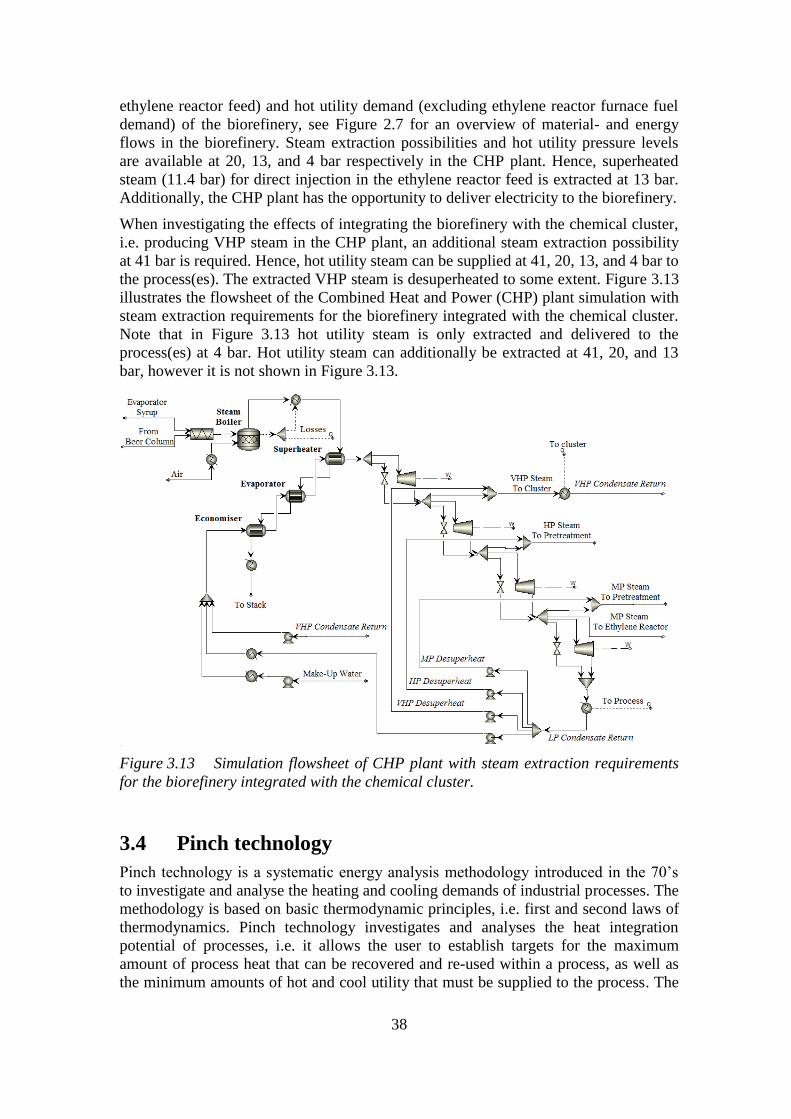
38

ethylene reactor feed) and hot utility demand (excluding ethylene reactor furnace fuel

demand) of the biorefinery, see Figure 2.7 for an overview of material- and energy

flows in the biorefinery. Steam extraction possibilities and hot utility pressure levels

are available at 20, 13, and 4 bar respectively in the CHP plant. Hence, superheated

steam (11.4 bar) for direct injection in the ethylene reactor feed is extracted at 13 bar.

Additionally, the CHP plant has the opportunity to deliver electricity to the biorefinery.

When investigating the effects of integrating the biorefinery with the chemical cluster,

i.e. producing VHP steam in the CHP plant, an additional steam extraction possibility

at 41 bar is required. Hence, hot utility steam can be supplied at 41, 20, 13, and 4 bar to

the process(es). The extracted VHP steam is desuperheated to some extent. Figure 3.13

illustrates the flowsheet of the Combined Heat and Power (CHP) plant simulation with

steam extraction requirements for the biorefinery integrated with the chemical cluster.

Note that in Figure 3.13 hot utility steam is only extracted and delivered to the

process(es) at 4 bar. Hot utility steam can additionally be extracted at 41, 20, and 13

bar, however it is not shown in Figure 3.13.

Figure 3.13 Simulation flowsheet of CHP plant with steam extraction requirements

for the biorefinery integrated with the chemical cluster.

3.4 Pinch technology

Pinch technology is a systematic energy analysis methodology introduced in the 70’s

to investigate and analyse the heating and cooling demands of industrial processes. The

methodology is based on basic thermodynamic principles, i.e. first and second laws of

thermodynamics. Pinch technology investigates and analyses the heat integration

potential of processes, i.e. it allows the user to establish targets for the maximum

amount of process heat that can be recovered and re-used within a process, as well as

the minimum amounts of hot and cool utility that must be supplied to the process. The

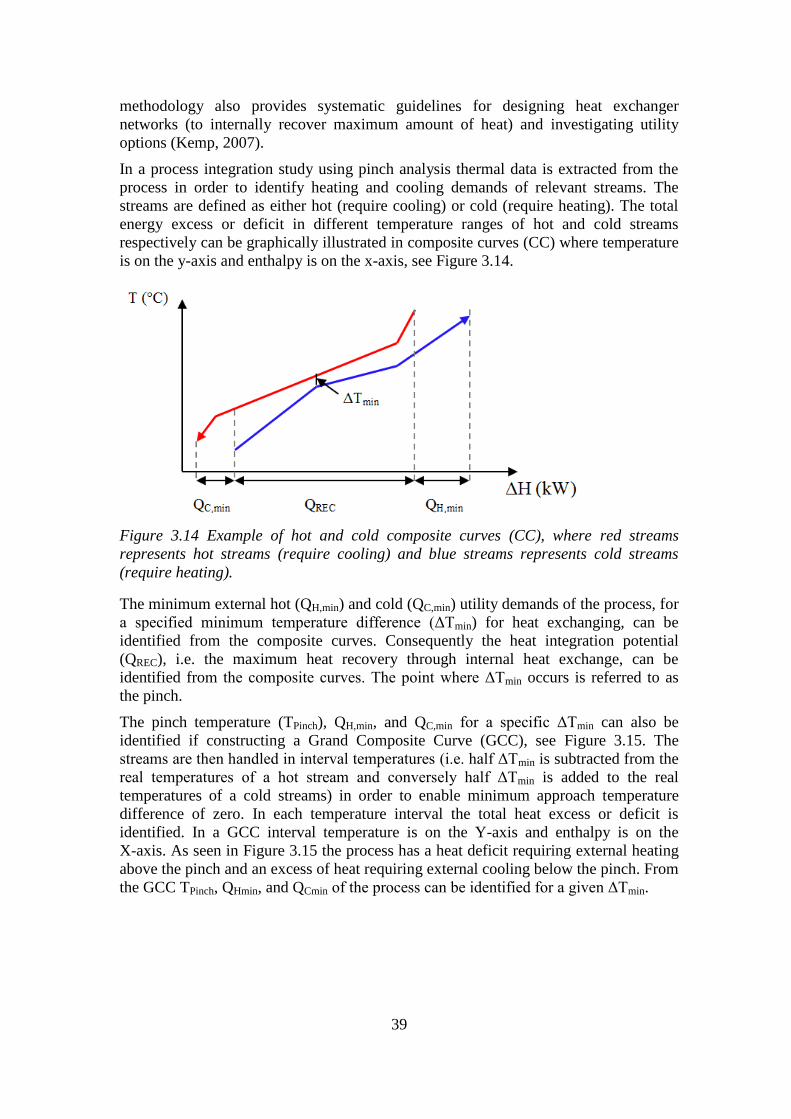
39

methodology also provides systematic guidelines for designing heat exchanger

networks (to internally recover maximum amount of heat) and investigating utility

options (Kemp, 2007).

In a process integration study using pinch analysis thermal data is extracted from the

process in order to identify heating and cooling demands of relevant streams. The

streams are defined as either hot (require cooling) or cold (require heating). The total

energy excess or deficit in different temperature ranges of hot and cold streams

respectively can be graphically illustrated in composite curves (CC) where temperature

is on the y-axis and enthalpy is on the x-axis, see Figure 3.14.

Figure 3.14 Example of hot and cold composite curves (CC), where red streams

represents hot streams (require cooling) and blue streams represents cold streams

(require heating).

The minimum external hot (QH,min) and cold (QC,min) utility demands of the process, for

a specified minimum temperature difference (ΔTmin) for heat exchanging, can be

identified from the composite curves. Consequently the heat integration potential

(QREC), i.e. the maximum heat recovery through internal heat exchange, can be

identified from the composite curves. The point where ΔTmin occurs is referred to as

the pinch.

The pinch temperature (TPinch), QH,min, and QC,min for a specific ΔTmin can also be

identified if constructing a Grand Composite Curve (GCC), see Figure 3.15. The

streams are then handled in interval temperatures (i.e. half ΔTmin is subtracted from the

real temperatures of a hot stream and conversely half ΔTmin is added to the real

temperatures of a cold streams) in order to enable minimum approach temperature

difference of zero. In each temperature interval the total heat excess or deficit is

identified. In a GCC interval temperature is on the Y-axis and enthalpy is on the

X-axis. As seen in Figure 3.15 the process has a heat deficit requiring external heating

above the pinch and an excess of heat requiring external cooling below the pinch. From

the GCC TPinch, QHmin, and QCmin of the process can be identified for a given ΔTmin.

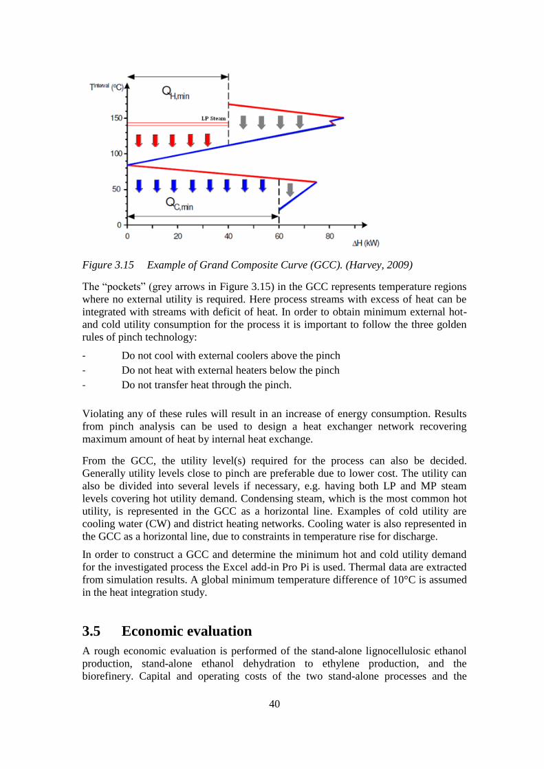
40

Figure 3.15 Example of Grand Composite Curve (GCC). (Harvey, 2009)

The “pockets” (grey arrows in Figure 3.15) in the GCC represents temperature regions

where no external utility is required. Here process streams with excess of heat can be

integrated with streams with deficit of heat. In order to obtain minimum external hot-

and cold utility consumption for the process it is important to follow the three golden

rules of pinch technology:

- Do not cool with external coolers above the pinch

- Do not heat with external heaters below the pinch

- Do not transfer heat through the pinch.

Violating any of these rules will result in an increase of energy consumption. Results

from pinch analysis can be used to design a heat exchanger network recovering

maximum amount of heat by internal heat exchange.

From the GCC, the utility level(s) required for the process can also be decided.

Generally utility levels close to pinch are preferable due to lower cost. The utility can

also be divided into several levels if necessary, e.g. having both LP and MP steam

levels covering hot utility demand. Condensing steam, which is the most common hot

utility, is represented in the GCC as a horizontal line. Examples of cold utility are

cooling water (CW) and district heating networks. Cooling water is also represented in

the GCC as a horizontal line, due to constraints in temperature rise for discharge.

In order to construct a GCC and determine the minimum hot and cold utility demand

for the investigated process the Excel add-in Pro Pi is used. Thermal data are extracted

from simulation results. A global minimum temperature difference of 10°C is assumed

in the heat integration study.

3.5 Economic evaluation

A rough economic evaluation is performed of the stand-alone lignocellulosic ethanol

production, stand-alone ethanol dehydration to ethylene production, and the

biorefinery. Capital and operating costs of the two stand-alone processes and the

41

biorefinery are estimated. Additionally, revenues are included to estimate the

production costs of ethanol and ethylene respectively through discounted cash flow

analysis. The production cost of ethanol and ethylene are estimated by determining the

equipment capital cost and operating (fixed and variable) costs of the two stand-alone

production plants and the biorefinery. Costs for the lignocellulosic ethanol production

are estimated using equipment cost correlations in the literature (Hamelinck, et al.,

2005; Aden, et al., 2002; Harvey, 2009) and simulation results. Costs for the ethanol

dehydration plant are based on correlations found in the literature (Jones, et al., 2010).

The economic evaluation is based on the assumption of 85421 operating hours of the

biorefinery annually.

3.5.1 Total capital cost estimation

Equipment costs for lignocellulosic ethanol production are estimated according to the

capacity power law expression in equation (3.1) (Harvey, 2009).

(

)

(3.1)

- Equipment cost for capacity

- Base equipment cost for capacity

- Scaling factor

Where , , and are obtained from the literature (Hamelinck, et al., 2005; Aden,

et al., 2002; Harvey, 2009) and is obtained from simulation results for each

equipment unit respectively. In order to obtain the total capital cost for lignocellulosic

ethanol production, an installation factor (accounting for designing, engineering,

construction, etc) for each equipment unit (Hamelinck, et al., 2005; Aden, et al., 2002;

Harvey, 2009) is multiplied with the corresponding equipment cost. In order to up-date

old data obtained from literature in the equipment cost estimation to year 2010

Chemical Engineering (CE) Index is used. Capital costs for storage- and wastewater

treatment facility, or pellets production are not included in the estimated total capital

cost for lignocellulosic ethanol production. Heat exchangers not included in major unit

operations (e.g. distillation reboilers, evaporation boiler, etc) are not accounted for in

the capital cost estimation.

Total capital costs for ethanol dehydration to ethylene production are estimated from a

power law expression based on plant capacity and data are obtained from the literature

(Jones, et al., 2010). The CE Index is used to update literature data to year 2010. An

average of a low and high investment scenario and a capacity of 200 000 tonne/year of

ethylene are assumed.

Total capital cost for the biorefinery producing ethylene from lignocellulosic feedstock

are estimated as the combined costs for the ethanol and ethylene production with

corresponding equipment requirements.

1Based on ethylene production rate of biorefinery simulation (i.e. 23.415 tonne/h) and production

requirement of 200 000 tonnes ethylene annually.

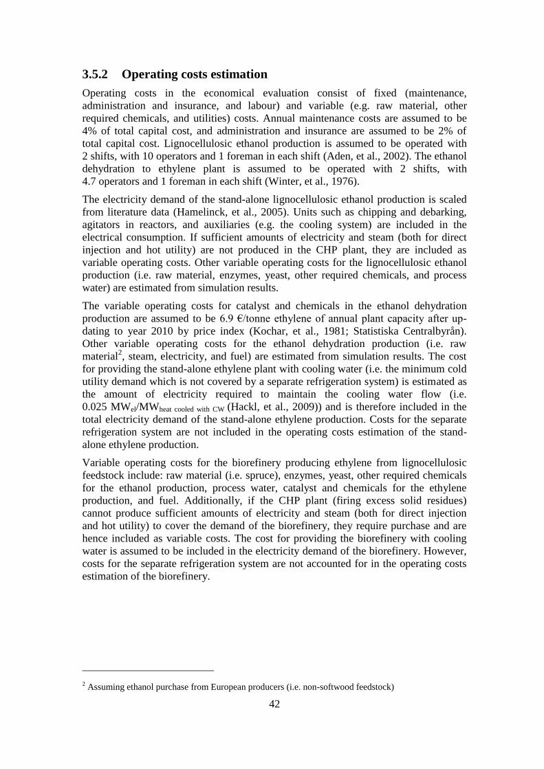
42

3.5.2 Operating costs estimation

Operating costs in the economical evaluation consist of fixed (maintenance,

administration and insurance, and labour) and variable (e.g. raw material, other

required chemicals, and utilities) costs. Annual maintenance costs are assumed to be

4% of total capital cost, and administration and insurance are assumed to be 2% of

total capital cost. Lignocellulosic ethanol production is assumed to be operated with

2 shifts, with 10 operators and 1 foreman in each shift (Aden, et al., 2002). The ethanol

dehydration to ethylene plant is assumed to be operated with 2 shifts, with

4.7 operators and 1 foreman in each shift (Winter, et al., 1976).

The electricity demand of the stand-alone lignocellulosic ethanol production is scaled

from literature data (Hamelinck, et al., 2005). Units such as chipping and debarking,

agitators in reactors, and auxiliaries (e.g. the cooling system) are included in the

electrical consumption. If sufficient amounts of electricity and steam (both for direct

injection and hot utility) are not produced in the CHP plant, they are included as

variable operating costs. Other variable operating costs for the lignocellulosic ethanol

production (i.e. raw material, enzymes, yeast, other required chemicals, and process

water) are estimated from simulation results.

The variable operating costs for catalyst and chemicals in the ethanol dehydration

production are assumed to be 6.9 €/tonne ethylene of annual plant capacity after up-

dating to year 2010 by price index (Kochar, et al., 1981; Statistiska Centralbyrån).

Other variable operating costs for the ethanol dehydration production (i.e. raw

material2, steam, electricity, and fuel) are estimated from simulation results. The cost

for providing the stand-alone ethylene plant with cooling water (i.e. the minimum cold

utility demand which is not covered by a separate refrigeration system) is estimated as

the amount of electricity required to maintain the cooling water flow (i.e.

0.025 MWel/MWheat cooled with CW (Hackl, et al., 2009)) and is therefore included in the

total electricity demand of the stand-alone ethylene production. Costs for the separate

refrigeration system are not included in the operating costs estimation of the stand-

alone ethylene production.

Variable operating costs for the biorefinery producing ethylene from lignocellulosic

feedstock include: raw material (i.e. spruce), enzymes, yeast, other required chemicals

for the ethanol production, process water, catalyst and chemicals for the ethylene

production, and fuel. Additionally, if the CHP plant (firing excess solid residues)

cannot produce sufficient amounts of electricity and steam (both for direct injection

and hot utility) to cover the demand of the biorefinery, they require purchase and are

hence included as variable costs. The cost for providing the biorefinery with cooling

water is assumed to be included in the electricity demand of the biorefinery. However,

costs for the separate refrigeration system are not accounted for in the operating costs

estimation of the biorefinery.

2 Assuming ethanol purchase from European producers (i.e. non-softwood feedstock)

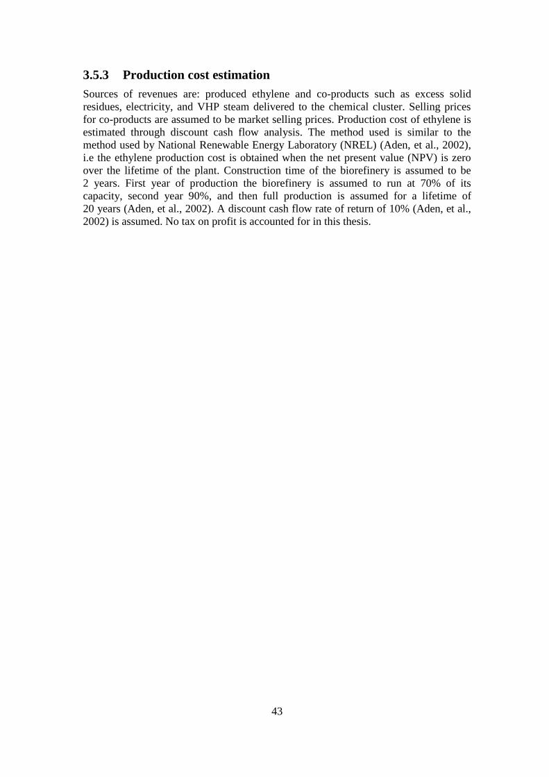
43

3.5.3 Production cost estimation

Sources of revenues are: produced ethylene and co-products such as excess solid

residues, electricity, and VHP steam delivered to the chemical cluster. Selling prices

for co-products are assumed to be market selling prices. Production cost of ethylene is

estimated through discount cash flow analysis. The method used is similar to the

method used by National Renewable Energy Laboratory (NREL) (Aden, et al., 2002),

i.e the ethylene production cost is obtained when the net present value (NPV) is zero

over the lifetime of the plant. Construction time of the biorefinery is assumed to be

2 years. First year of production the biorefinery is assumed to run at 70% of its

capacity, second year 90%, and then full production is assumed for a lifetime of

20 years (Aden, et al., 2002). A discount cash flow rate of return of 10% (Aden, et al.,

2002) is assumed. No tax on profit is accounted for in this thesis.

45

4 Results and Discussion

4.1 Simulation results

4.1.1 Stand-alone lignocellulosic ethanol production

Figure 4.1 presents material balance results obtained from the Aspen Plus simulation

model of the stand-alone lignocellulosic ethanol production (i.e. the process

configuration described in Section 2.1.2). In Figure 4.1 the main energy flows are also

represented (e.g. biomass input, direct steam injection requirements in pretreatment,

ethanol output, etc).

The load of the lignin-rich solid residues (i.e. combined slurry of the solid fraction

from the beer column and the concentrated evaporation syrup) to the CHP plant is set

to cover the minimum hot utility demand (112 MW) of the stand-alone lignocellulosic

ethanol production obtained in the heat integration study (see Section 4.2.1). The

resulting amount of excess solid residues after covering the minimum hot utility and

steam for direct injection in the pretreatment steps is estimated at 86 MW, and the

co-generated electricity is estimated at 56 MWel, see Figure 4.1.

Figure 4.1 Material and main energy balance results for the stand-alone

lignocellulosic ethanol production simulation. Energy flows are estimated in Aspen

Plus based on High Heating Values (HHV). SSCF – Simultaneous Saccharification

and Co-Fermentation, (S) – Solid Fraction, (L) – Liquid Fraction, (C) – Condensate.

In Figure 4.1 the most energy demanding process steps in the stand-alone

lignocellulosic ethanol production are represented, which are also summarised in

Table 4.1.

46

Table 4.1 Most energy demanding unit operations in the ethanol production.

Unit Operation MW Unit Operation MW

Pretreatment 1 (MP) 42.1 Beer column reboiler 48.8

Pretreatment 2 (HP) 9.1 Rectifier reboiler 17.9

Preheater beer column 41.8 Evaporation 41.8

Table 4.2 presents key results obtained from simulation of the stand-alone

lignocellulosic ethanol production plant. The stand-alone ethanol production plant

produces 43.9 tonne ethanol (93 wt%) per hour, which corresponds to a yield of

277.6 kg ethanol per tonne dry wood. As discussed in Section 2.1.5, the theoretical

amount of ethanol that can be derived from assumed feedstock composition is

383 kg/tonne dry wood (i.e. 336 kg/tonne dry wood and 47 kg/tonne dry wood from

hexoses and pentoses respectively). Hence, the obtained overall ethanol yield (of

theoretical) is 72.5%. As mentioned in Section 2.1.6, the ethanol concentration in the

beer column feed greatly affects the energy demand of the column (higher ethanol feed

concentration results in lower reboiler duty). The obtained ethanol feed concentration

to beer column (6.7 wt%) is considered relatively high when handling lignocellulosic

feedstock. After combining the solid fraction of the beer column stillage and the

concentrated evaporation syrup, a moisture content of 41.8 wt% is obtained.

Table 4.2 Simulation results for the stand-alone ethanol production plant.

Produced ethanol (93%) 43875 kg/h

Ethanol yield (kg ethanol / tonne dry wood) 277.6 kg/tonne

Overall ethanol yield (of theoretical) 72.5 %

Ethanol concentration before beer column 6.7 wt%

Ethanol concentration to rectifier 49.0 wt%

Moisture content of solid residues to CHP plant 41.8 wt%


Figure 4.2 presents material balance results from the Aspen Plus simulation model of

the stand-alone ethanol dehydration to ethylene production (i.e. the process

configuration described in Section 2.2.1). In Figure 4.2 the main energy flows are also

represented (e.g. ethanol input, direct steam injection requirements to reactor feed,

ethylene output, etc). It should be noted that the MP steam required for direct injection

into ethylene reactor feed need to be produced externally. The required amount of

external fuel to the furnace (after firing of by-products) is dependent on the results

obtained from the heat integration study (see Section 4.2.2).

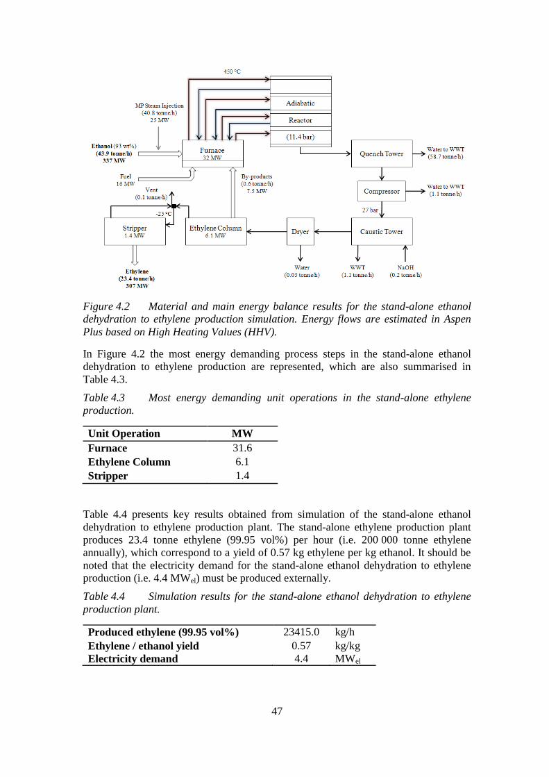
47

Figure 4.2 Material and main energy balance results for the stand-alone ethanol

dehydration to ethylene production simulation. Energy flows are estimated in Aspen

Plus based on High Heating Values (HHV).

In Figure 4.2 the most energy demanding process steps in the stand-alone ethanol

dehydration to ethylene production are represented, which are also summarised in

Table 4.3.

Table 4.3 Most energy demanding unit operations in the stand-alone ethylene

production.

Unit Operation MW

Furnace 31.6

Ethylene Column 6.1

Stripper 1.4

Table 4.4 presents key results obtained from simulation of the stand-alone ethanol

dehydration to ethylene production plant. The stand-alone ethylene production plant

produces 23.4 tonne ethylene (99.95 vol%) per hour (i.e. 200 000 tonne ethylene

annually), which correspond to a yield of 0.57 kg ethylene per kg ethanol. It should be

noted that the electricity demand for the stand-alone ethanol dehydration to ethylene

production (i.e. 4.4 MWel) must be produced externally.

Table 4.4 Simulation results for the stand-alone ethanol dehydration to ethylene

production plant.

Produced ethylene (99.95 vol%) 23415.0 kg/h

Ethylene / ethanol yield

Electricity demand

0.57

4.4

kg/kg

MWel

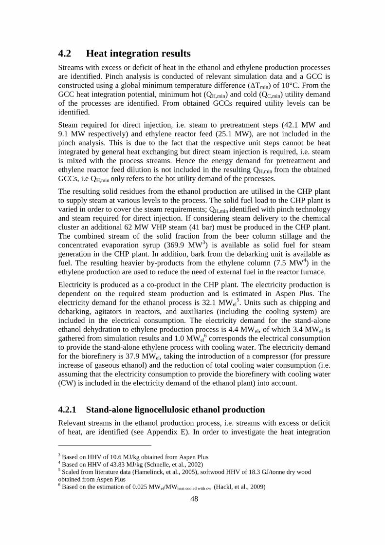
48

4.2 Heat integration results

Streams with excess or deficit of heat in the ethanol and ethylene production processes

are identified. Pinch analysis is conducted of relevant simulation data and a GCC is

constructed using a global minimum temperature difference (ΔTmin) of 10°C. From the

GCC heat integration potential, minimum hot (QH,min) and cold (QC,min) utility demand

of the processes are identified. From obtained GCCs required utility levels can be

identified.

Steam required for direct injection, i.e. steam to pretreatment steps (42.1 MW and

9.1 MW respectively) and ethylene reactor feed (25.1 MW), are not included in the

pinch analysis. This is due to the fact that the respective unit steps cannot be heat

integrated by general heat exchanging but direct steam injection is required, i.e. steam

is mixed with the process streams. Hence the energy demand for pretreatment and

ethylene reactor feed dilution is not included in the resulting QH,min from the obtained

GCCs, i.e QH,min only refers to the hot utility demand of the processes.

The resulting solid residues from the ethanol production are utilised in the CHP plant

to supply steam at various levels to the process. The solid fuel load to the CHP plant is

varied in order to cover the steam requirements; QH,min identified with pinch technology

and steam required for direct injection. If considering steam delivery to the chemical

cluster an additional 62 MW VHP steam (41 bar) must be produced in the CHP plant.

The combined stream of the solid fraction from the beer column stillage and the

concentrated evaporation syrup (369.9 MW3) is available as solid fuel for steam

generation in the CHP plant. In addition, bark from the debarking unit is available as

fuel. The resulting heavier by-products from the ethylene column (7.5 MW4) in the

ethylene production are used to reduce the need of external fuel in the reactor furnace.

Electricity is produced as a co-product in the CHP plant. The electricity production is

dependent on the required steam production and is estimated in Aspen Plus. The

electricity demand for the ethanol process is 32.1 MWel5. Units such as chipping and

debarking, agitators in reactors, and auxiliaries (including the cooling system) are

included in the electrical consumption. The electricity demand for the stand-alone

ethanol dehydration to ethylene production process is 4.4 MWel, of which 3.4 MWel is

gathered from simulation results and 1.0 MWel6 corresponds the electrical consumption

to provide the stand-alone ethylene process with cooling water. The electricity demand

for the biorefinery is 37.9 MWel, taking the introduction of a compressor (for pressure

increase of gaseous ethanol) and the reduction of total cooling water consumption (i.e.

assuming that the electricity consumption to provide the biorefinery with cooling water

(CW) is included in the electricity demand of the ethanol plant) into account.

4.2.1 Stand-alone lignocellulosic ethanol production

Relevant streams in the ethanol production process, i.e. streams with excess or deficit

of heat, are identified (see Appendix E). In order to investigate the heat integration

3 Based on HHV of 10.6 MJ/kg obtained from Aspen Plus

4 Based on HHV of 43.83 MJ/kg (Schnelle, et al., 2002)

5 Scaled from literature data (Hamelinck, et al., 2005), softwood HHV of 18.3 GJ/tonne dry wood

obtained from Aspen Plus 6 Based on the estimation of 0.025 MWel/MWheat cooled with cw (Hackl, et al., 2009)

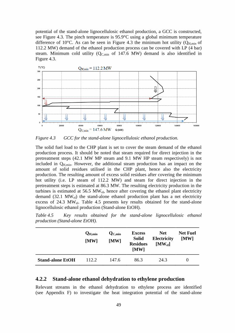
49

potential of the stand-alone lignocellulosic ethanol production, a GCC is constructed,

see Figure 4.3. The pinch temperature is 95.9°C using a global minimum temperature

difference of 10°C. As can be seen in Figure 4.3 the minimum hot utility (QH,min of

112.2 MW) demand of the ethanol production process can be covered with LP (4 bar)

steam. Minimum cold utility (QC,min of 147.6 MW) demand is also identified in

Figure 4.3.

Figure 4.3 GCC for the stand-alone lignocellulosic ethanol production.

The solid fuel load to the CHP plant is set to cover the steam demand of the ethanol

production process. It should be noted that steam required for direct injection in the

pretreatment steps (42.1 MW MP steam and 9.1 MW HP steam respectively) is not

included in QH,min. However, the additional steam production has an impact on the

amount of solid residues utilised in the CHP plant, hence also the electricity

production. The resulting amount of excess solid residues after covering the minimum

hot utility (i.e. LP steam of 112.2 MW) and steam for direct injection in the

pretreatment steps is estimated at 86.3 MW. The resulting electricity production in the

turbines is estimated at 56.5 MWel, hence after covering the ethanol plant electricity

demand (32.1 MWel) the stand-alone ethanol production plant has a net electricity

excess of 24.3 MWel. Table 4.5 presents key results obtained for the stand-alone

lignocellulosic ethanol production (Stand-alone EtOH).

Table 4.5 Key results obtained for the stand-alone lignocellulosic ethanol

production (Stand-alone EtOH).

QH,min

[MW]

QC,min

[MW]

Excess

Solid

Residues

[MW]

Net

Electricity

[MWel]

Net Fuel

[MW]

Stand-alone EtOH 112.2 147.6 86.3 24.3 0


Relevant streams in the ethanol dehydration to ethylene process are identified

(see Appendix F) to investigate the heat integration potential of the stand-alone

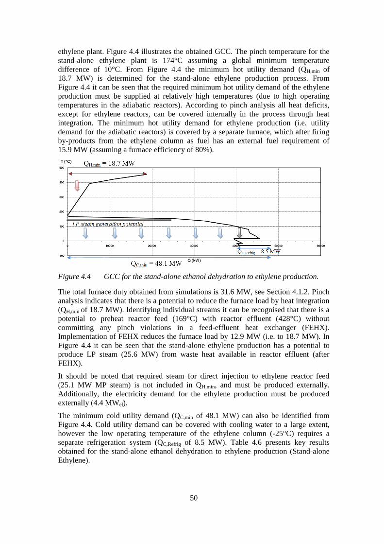
50

ethylene plant. Figure 4.4 illustrates the obtained GCC. The pinch temperature for the

stand-alone ethylene plant is 174°C assuming a global minimum temperature

difference of 10°C. From Figure 4.4 the minimum hot utility demand (QH,min of

18.7 MW) is determined for the stand-alone ethylene production process. From

Figure 4.4 it can be seen that the required minimum hot utility demand of the ethylene

production must be supplied at relatively high temperatures (due to high operating

temperatures in the adiabatic reactors). According to pinch analysis all heat deficits,

except for ethylene reactors, can be covered internally in the process through heat

integration. The minimum hot utility demand for ethylene production (i.e. utility

demand for the adiabatic reactors) is covered by a separate furnace, which after firing

by-products from the ethylene column as fuel has an external fuel requirement of

15.9 MW (assuming a furnace efficiency of 80%).

Figure 4.4 GCC for the stand-alone ethanol dehydration to ethylene production.

The total furnace duty obtained from simulations is 31.6 MW, see Section 4.1.2. Pinch

analysis indicates that there is a potential to reduce the furnace load by heat integration

(QH,min of 18.7 MW). Identifying individual streams it can be recognised that there is a

potential to preheat reactor feed (169°C) with reactor effluent (428°C) without

committing any pinch violations in a feed-effluent heat exchanger (FEHX).

Implementation of FEHX reduces the furnace load by 12.9 MW (i.e. to 18.7 MW). In

Figure 4.4 it can be seen that the stand-alone ethylene production has a potential to

produce LP steam (25.6 MW) from waste heat available in reactor effluent (after

FEHX).

It should be noted that required steam for direct injection to ethylene reactor feed

(25.1 MW MP steam) is not included in QH,min, and must be produced externally.

Additionally, the electricity demand for the ethylene production must be produced

externally (4.4 MWel).

The minimum cold utility demand (QC,min of 48.1 MW) can also be identified from

Figure 4.4. Cold utility demand can be covered with cooling water to a large extent,

however the low operating temperature of the ethylene column (-25°C) requires a

separate refrigeration system (QC,Refrig of 8.5 MW). Table 4.6 presents key results

obtained for the stand-alone ethanol dehydration to ethylene production (Stand-alone

Ethylene).

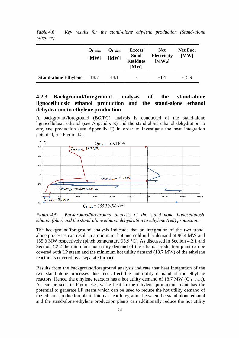
51

Table 4.6 Key results for the stand-alone ethylene production (Stand-alone

Ethylene).

QH,min

[MW]

QC,min

[MW]

Excess

Solid

Residues

[MW]

Net

Electricity

[MWel]

Net Fuel

[MW]

Stand-alone Ethylene 18.7 48.1 - -4.4 -15.9

4.2.3 Background/foreground analysis of the stand-alone

lignocellulosic ethanol production and the stand-alone ethanol

dehydration to ethylene production

A background/foreground (BG/FG) analysis is conducted of the stand-alone

lignocellulosic ethanol (see Appendix E) and the stand-alone ethanol dehydration to

ethylene production (see Appendix F) in order to investigate the heat integration

potential, see Figure 4.5.

Figure 4.5 Background/foreground analysis of the stand-alone lignocellulosic

ethanol (blue) and the stand-alone ethanol dehydration to ethylene (red) production.

The background/foreground analysis indicates that an integration of the two stand-

alone processes can result in a minimum hot and cold utility demand of 90.4 MW and

155.3 MW respectively (pinch temperature 95.9 °C). As discussed in Section 4.2.1 and

Section 4.2.2 the minimum hot utility demand of the ethanol production plant can be

covered with LP steam and the minimum hot utility demand (18.7 MW) of the ethylene

reactors is covered by a separate furnace.

Results from the background/foreground analysis indicate that heat integration of the

two stand-alone processes does not affect the hot utility demand of the ethylene

reactors. Hence, the ethylene reactors has a hot utility demand of 18.7 MW (QH,furnace).

As can be seen in Figure 4.5, waste heat in the ethylene production plant has the

potential to generate LP steam which can be used to reduce the hot utility demand of

the ethanol production plant. Internal heat integration between the stand-alone ethanol

and the stand-alone ethylene production plants can additionally reduce the hot utility

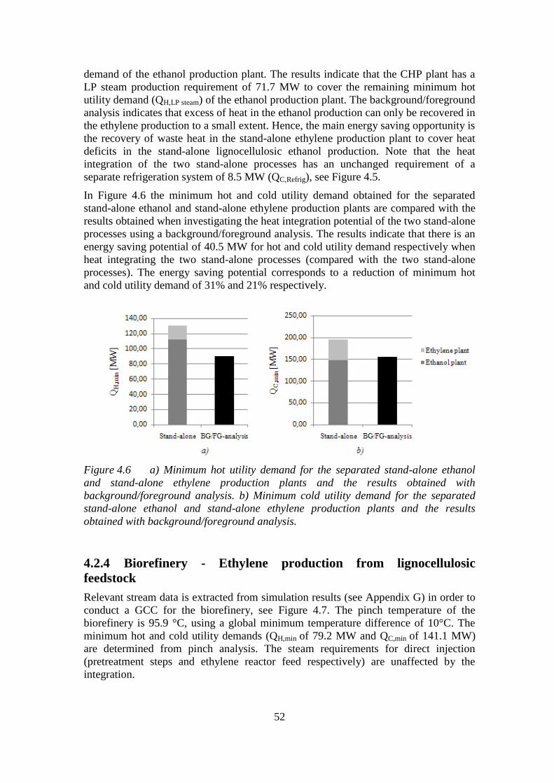
52

demand of the ethanol production plant. The results indicate that the CHP plant has a

LP steam production requirement of 71.7 MW to cover the remaining minimum hot

utility demand (QH,LP steam) of the ethanol production plant. The background/foreground

analysis indicates that excess of heat in the ethanol production can only be recovered in

the ethylene production to a small extent. Hence, the main energy saving opportunity is

the recovery of waste heat in the stand-alone ethylene production plant to cover heat

deficits in the stand-alone lignocellulosic ethanol production. Note that the heat

integration of the two stand-alone processes has an unchanged requirement of a

separate refrigeration system of 8.5 MW (QC,Refrig), see Figure 4.5.

In Figure 4.6 the minimum hot and cold utility demand obtained for the separated

stand-alone ethanol and stand-alone ethylene production plants are compared with the

results obtained when investigating the heat integration potential of the two stand-alone

processes using a background/foreground analysis. The results indicate that there is an

energy saving potential of 40.5 MW for hot and cold utility demand respectively when

heat integrating the two stand-alone processes (compared with the two stand-alone

processes). The energy saving potential corresponds to a reduction of minimum hot

and cold utility demand of 31% and 21% respectively.

Figure 4.6 a) Minimum hot utility demand for the separated stand-alone ethanol

and stand-alone ethylene production plants and the results obtained with

background/foreground analysis. b) Minimum cold utility demand for the separated

stand-alone ethanol and stand-alone ethylene production plants and the results

obtained with background/foreground analysis.

4.2.4 Biorefinery - Ethylene production from lignocellulosic

feedstock

Relevant stream data is extracted from simulation results (see Appendix G) in order to

conduct a GCC for the biorefinery, see Figure 4.7. The pinch temperature of the

biorefinery is 95.9 °C, using a global minimum temperature difference of 10°C. The

minimum hot and cold utility demands (QH,min of 79.2 MW and QC,min of 141.1 MW)

are determined from pinch analysis. The steam requirements for direct injection

(pretreatment steps and ethylene reactor feed respectively) are unaffected by the

integration.

53

Figure 4.7 GCC for biorefinery producing ethylene from lignocellulosic feedstock.

As described in Chapter 3.3, the pressure increase of the ethylene reactor feed is

achieved by compression when stand-alone ethanol and ethylene production are

integrated into a biorefinery (due to the fact that ethanol is delivered in gas phase). As

a result ethanol is delivered to the ethylene plant at a higher temperature reducing the

FEHX load from 12.9 MW to 10.6 MW and the furnace load from 18.7 MW to

12.4 MW (which after utilisation of by-products has an external fuel requirement of

7.9 MW, assuming a furnace efficiency of 80%). As a consequence of the FEHX load

reduction the LP steam generation potential is increased to 27.8 MW. However when

ethanol is delivered directly to the ethylene plant the pressure is increased with a

compressor instead of a pump, which increases the electricity demand of the

biorefinery by 2.4 MWel. Additionally, the electricity consumption for providing the

biorefinery with sufficient amount of cooling water is taken in into consideration (i.e. it

is assumed to be included in the electricity demand estimation of the ethanol plant).

The total electricity demand for the biorefinery is then 37.9 MWel.

Accordingly, the hot utility demand for the ethylene reactors is covered by external

fuel (QH,furnace of 12.4 MW) in a separate furnace and the remaining hot utility demand

of the biorefinery can be covered with LP steam (QH,LP steam of 66.8 MW), see

Figure 4.7. The integration opportunity to produce LP steam from waste heat (i.e. from

ethylene reactor effluent) and deliver it to the ethanol process can be identified in the

pocket at 146°C in Figure 4.7. It should be noted that in the temperature interval of the

pocket in Figure 4.7 other streams are also included (e.g. flash steam after pretreatment

steps in the ethanol production). Note that the heat integration of the two stand-alone

processes into a biorefinery producing ethylene from lignocellulosic feedstock has an

unchanged requirement of a separate refrigeration system of 8.5 MW (QC,Refrig), see

Figure 4.7.

Utility steam and steam for direct injection (i.e. pretreatment steps and ethylene reactor

feed respectively) requirements are covered by the CHP plant utilising lignin-rich

residues. After producing necessary steam to the process the biorefinery results in

123.1 MW of excess solid residues. Additionally 45.9 MWel are co-generated in the

CHP plant, which results in a net electricity production of 8.0 MWel after covering the

electricity demand of the biorefinery (i.e. 37.9 MWel). Table 4.7 presents key results

obtained for the biorefinery producing ethylene from lignocellulosic feedstock.

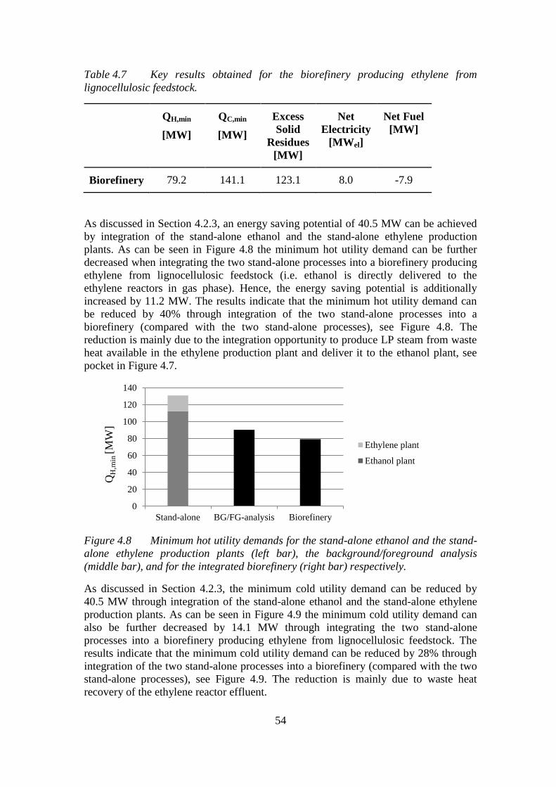
54

Table 4.7 Key results obtained for the biorefinery producing ethylene from

lignocellulosic feedstock.

QH,min

[MW]

QC,min

[MW]

Excess

Solid

Residues

[MW]

Net

Electricity

[MWel]

Net Fuel

[MW]

Biorefinery 79.2 141.1 123.1 8.0 -7.9

As discussed in Section 4.2.3, an energy saving potential of 40.5 MW can be achieved

by integration of the stand-alone ethanol and the stand-alone ethylene production

plants. As can be seen in Figure 4.8 the minimum hot utility demand can be further

decreased when integrating the two stand-alone processes into a biorefinery producing

ethylene from lignocellulosic feedstock (i.e. ethanol is directly delivered to the

ethylene reactors in gas phase). Hence, the energy saving potential is additionally

increased by 11.2 MW. The results indicate that the minimum hot utility demand can

be reduced by 40% through integration of the two stand-alone processes into a

biorefinery (compared with the two stand-alone processes), see Figure 4.8. The

reduction is mainly due to the integration opportunity to produce LP steam from waste

heat available in the ethylene production plant and deliver it to the ethanol plant, see

pocket in Figure 4.7.

Figure 4.8 Minimum hot utility demands for the stand-alone ethanol and the stand-

alone ethylene production plants (left bar), the background/foreground analysis

(middle bar), and for the integrated biorefinery (right bar) respectively.

As discussed in Section 4.2.3, the minimum cold utility demand can be reduced by

40.5 MW through integration of the stand-alone ethanol and the stand-alone ethylene

production plants. As can be seen in Figure 4.9 the minimum cold utility demand can

also be further decreased by 14.1 MW through integrating the two stand-alone

processes into a biorefinery producing ethylene from lignocellulosic feedstock. The

results indicate that the minimum cold utility demand can be reduced by 28% through

integration of the two stand-alone processes into a biorefinery (compared with the two

stand-alone processes), see Figure 4.9. The reduction is mainly due to waste heat

recovery of the ethylene reactor effluent.

0

20

40

60

80

100

120

140

Stand-alone BG/FG-analysis Biorefinery

QH

,min

[M

W]

Ethylene plant

Ethanol plant

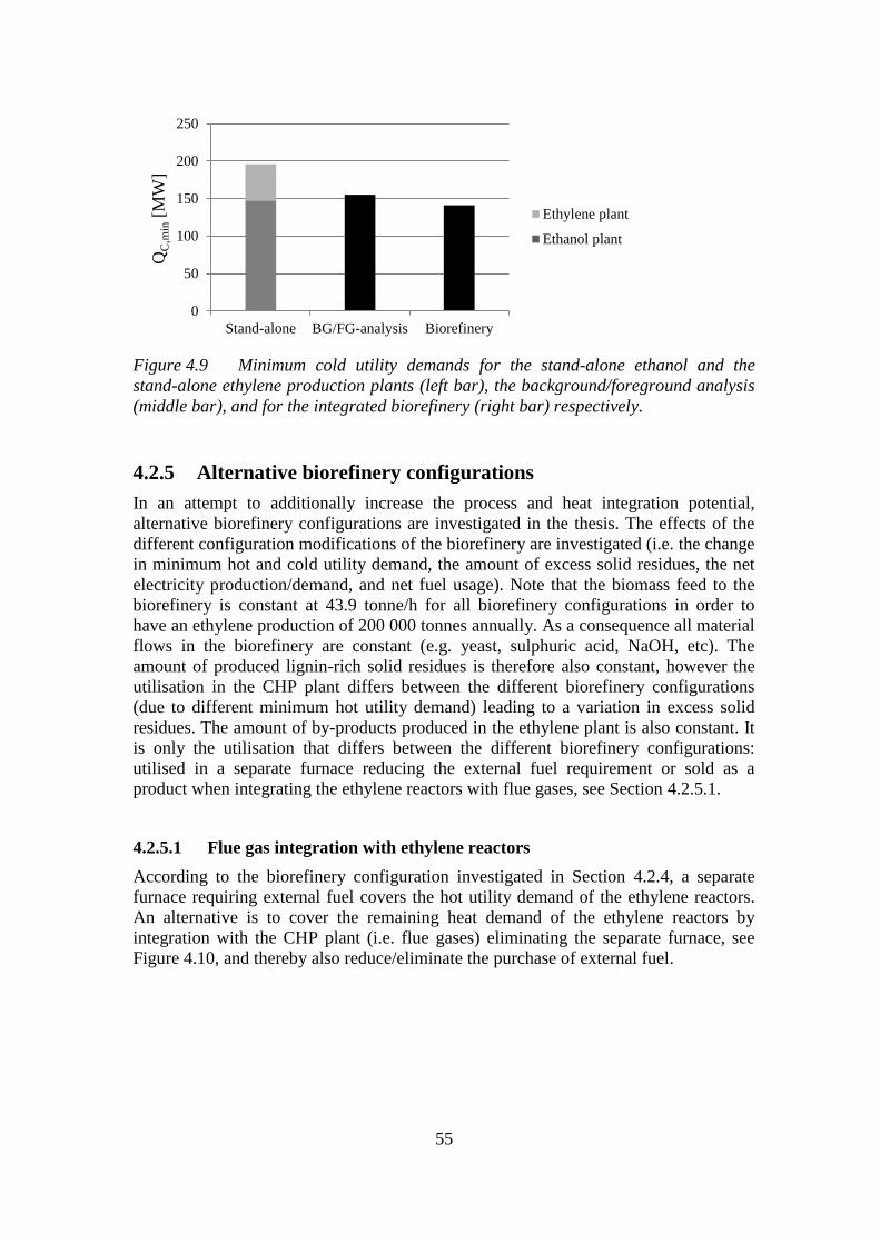
55

Figure 4.9 Minimum cold utility demands for the stand-alone ethanol and the

stand-alone ethylene production plants (left bar), the background/foreground analysis

(middle bar), and for the integrated biorefinery (right bar) respectively.

4.2.5 Alternative biorefinery configurations

In an attempt to additionally increase the process and heat integration potential,

alternative biorefinery configurations are investigated in the thesis. The effects of the

different configuration modifications of the biorefinery are investigated (i.e. the change

in minimum hot and cold utility demand, the amount of excess solid residues, the net

electricity production/demand, and net fuel usage). Note that the biomass feed to the

biorefinery is constant at 43.9 tonne/h for all biorefinery configurations in order to

have an ethylene production of 200 000 tonnes annually. As a consequence all material

flows in the biorefinery are constant (e.g. yeast, sulphuric acid, NaOH, etc). The

amount of produced lignin-rich solid residues is therefore also constant, however the

utilisation in the CHP plant differs between the different biorefinery configurations

(due to different minimum hot utility demand) leading to a variation in excess solid

residues. The amount of by-products produced in the ethylene plant is also constant. It

is only the utilisation that differs between the different biorefinery configurations:

utilised in a separate furnace reducing the external fuel requirement or sold as a

product when integrating the ethylene reactors with flue gases, see Section 4.2.5.1.

4.2.5.1 Flue gas integration with ethylene reactors

According to the biorefinery configuration investigated in Section 4.2.4, a separate

furnace requiring external fuel covers the hot utility demand of the ethylene reactors.

An alternative is to cover the remaining heat demand of the ethylene reactors by

integration with the CHP plant (i.e. flue gases) eliminating the separate furnace, see

Figure 4.10, and thereby also reduce/eliminate the purchase of external fuel.

0

50

100

150

200

250

Stand-alone BG/FG-analysis Biorefinery

QC

,min

[M

W]

Ethylene plant

Ethanol plant

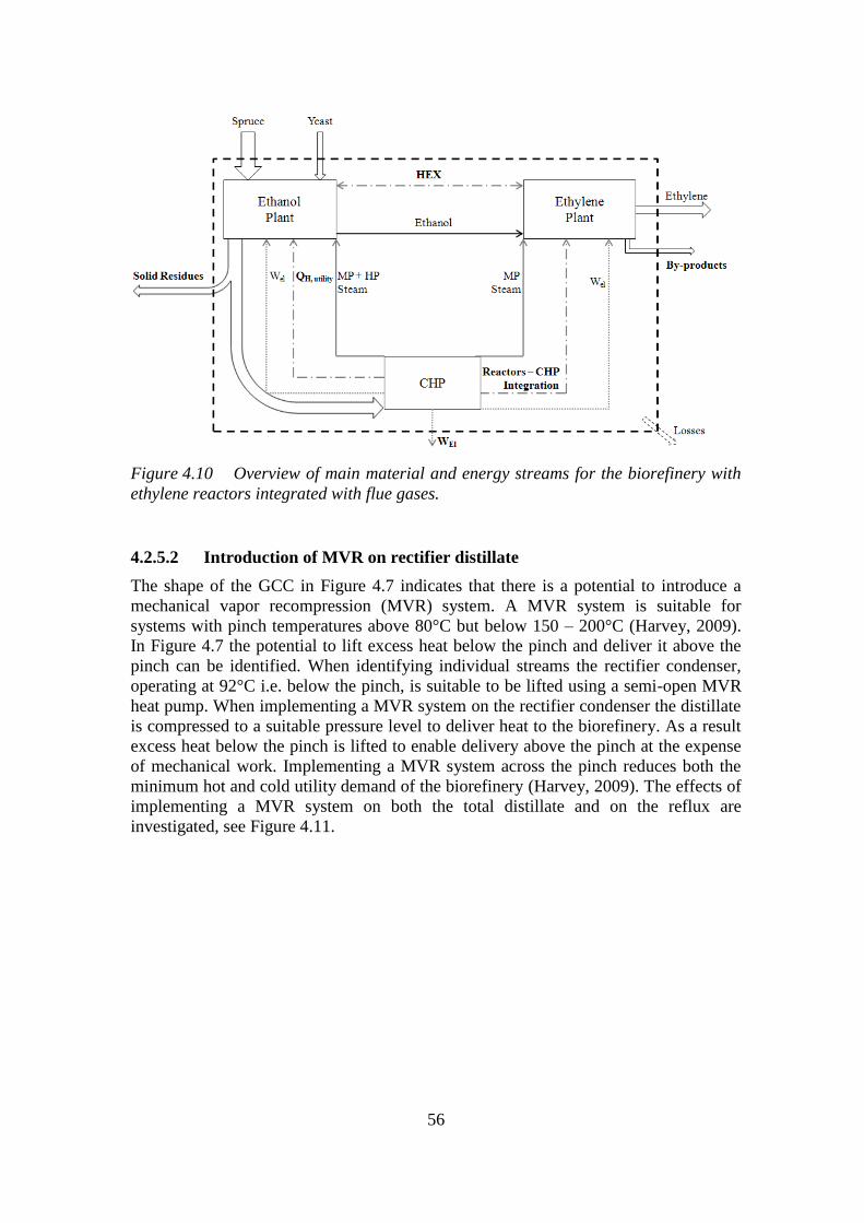
56

Figure 4.10 Overview of main material and energy streams for the biorefinery with

ethylene reactors integrated with flue gases.

4.2.5.2 Introduction of MVR on rectifier distillate

The shape of the GCC in Figure 4.7 indicates that there is a potential to introduce a

mechanical vapor recompression (MVR) system. A MVR system is suitable for

systems with pinch temperatures above 80°C but below 150 – 200°C (Harvey, 2009).

In Figure 4.7 the potential to lift excess heat below the pinch and deliver it above the

pinch can be identified. When identifying individual streams the rectifier condenser,

operating at 92°C i.e. below the pinch, is suitable to be lifted using a semi-open MVR

heat pump. When implementing a MVR system on the rectifier condenser the distillate

is compressed to a suitable pressure level to deliver heat to the biorefinery. As a result

excess heat below the pinch is lifted to enable delivery above the pinch at the expense

of mechanical work. Implementing a MVR system across the pinch reduces both the

minimum hot and cold utility demand of the biorefinery (Harvey, 2009). The effects of

implementing a MVR system on both the total distillate and on the reflux are

investigated, see Figure 4.11.

57

Figure 4.11 MVR configurations when implemented on the total distillate (left) and

when heat pumping the reflux (right).

The MVR efficiency can be measured with:

(4.1)

Where COP is the Coefficient of Performance, is useful heat delivered to the

process, and is the required compressor work. and are taken from

simulation results in order to estimate the COP of the MVR.

4.2.5.3 VHP (41 bar) steam delivery to the chemical cluster

As discussed in Section 2.4, results from a TSA study show that the chemical cluster in

Stenungsund has a heat deficit of 62 MW after site wide energy efficiency measures

which can be covered with VHP (41 bar) steam. The opportunity to produce a

sufficient amount of VHP steam (after covering the minimum hot utility demand and

steam demand for direct injection of the biorefinery) by utilisation of excess lignin-rich

solid residues is investigated in the thesis. The delivery of VHP steam to the chemical

cluster will result in an additional income to the biorefinery affecting the ethylene

production cost. However, it will occur at the expense of excess solid residues which

also provide an income source to the biorefinery. The integration opportunity will

contribute by reducing the degree of fossil fuel dependence of the biorefinery, as the

hot utility deficit is covered by “green” fuel.

4.2.6 Biorefinery – Flue gas integration with ethylene reactors

(Bio-F)

The effects of integrating the dehydration reactors with the flue gases of the CHP plant

are investigated (Bio-F). As a result the need of a separate furnace is eliminated and

the ethylene by-products can be sold as a product.

Sufficient energy to cover the energy demand in ethylene reactors (12.4 MW) is

extracted from the flue gases in the CHP plant. A ∆Tmin of 20°C is assumed in the heat

exchanging between the two gas streams. The extracted flue gas stream and the

ethylene reactors requiring hot utility are excluded in the pinch analysis, since no other

heat integration opportunity is desired to be investigated. As a consequence the hot

58

utility requirement for the ethylene reactors is excluded in the obtained minimum hot

utility demand for the Bio-F. The resulting GCC for the Bio-F is presented in

Figure 4.12.

Figure 4.12 GCC for the Bio-F.

The pinch temperature of the biorefinery configuration with flue gas integration with

the ethylene reactors (Bio-F) is 95.9 °C, using a global minimum temperature

difference of 10°C. As can be seen in Figure 4.12 the Bio-F has a minimum hot and

cold utility demand of 68.0 MW and 140.4 MW respectively. It can be seen in

Figure 4.12 that the hot utility demand of the Bio-F can be covered with LP steam. The

steam production in the CHP plant results in an excess of 105.0 MW lignin-rich solids

and an electricity production of 46.4 MWel (i.e. a net electricity production of

8.5 MWel). By-products produced (7.5 MW) in the ethylene plant have the potential to

be sold as product. Table 4.8 presents key results obtained for the Bio-F and the

Biorefinery (i.e. without any configuration modifications).

Table 4.8 Key results obtained for the Biorefinery and Bio-F.

QH,min

[MW]

QC,min

[MW]

Excess

Solid

Residues

[MW]

Net

Electricity

[MWel]

Net Fuel

[MW]

Biorefinery 79.2 141.1 123.1 8.0 -7.9

Bio-F 68.0 140.4 105.0 8.5 7.5

The results from the Bio-F indicate that it is possible to increase the capacity of the

CHP plant to cover the requirements of the dehydration reactors. However, this results

in a reduction of the amount of excess solid residues (i.e. reduction by 18 MW, see

Table 4.8). The capacity increase of the CHP plant results in an increased air

preheating demand. Consequently the LP steam demand of the Bio-F is increased

(QH,LP steam,Bio-F of 68.0 MW) compared with the Biorefinery (QH,LP steam,Biorefinery of

66.8 MW). As a consequence of the increased steam generation, the electricity

generation in the turbine is increased by 0.5 MWel in the CHP plant.

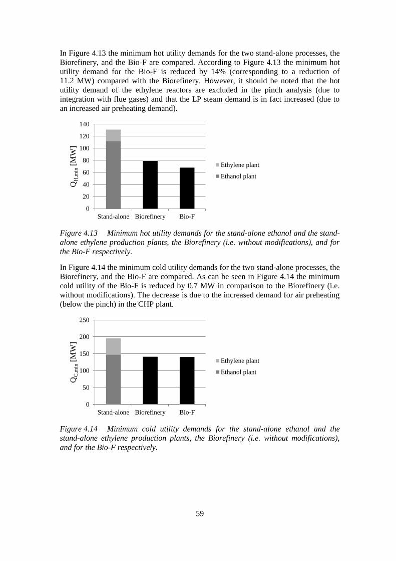
59

In Figure 4.13 the minimum hot utility demands for the two stand-alone processes, the

Biorefinery, and the Bio-F are compared. According to Figure 4.13 the minimum hot

utility demand for the Bio-F is reduced by 14% (corresponding to a reduction of

11.2 MW) compared with the Biorefinery. However, it should be noted that the hot

utility demand of the ethylene reactors are excluded in the pinch analysis (due to

integration with flue gases) and that the LP steam demand is in fact increased (due to

an increased air preheating demand).


alone ethylene production plants, the Biorefinery (i.e. without modifications), and for

the Bio-F respectively.

In Figure 4.14 the minimum cold utility demands for the two stand-alone processes, the

Biorefinery, and the Bio-F are compared. As can be seen in Figure 4.14 the minimum

cold utility of the Bio-F is reduced by 0.7 MW in comparison to the Biorefinery (i.e.

without modifications). The decrease is due to the increased demand for air preheating

(below the pinch) in the CHP plant.


stand-alone ethylene production plants, the Biorefinery (i.e. without modifications),

and for the Bio-F respectively.

0

20

40

60

80

100

120

140

Stand-alone Biorefinery Bio-F

QH

,min

[M

W]

Ethylene plant

Ethanol plant

0

50

100

150

200

250

Stand-alone Biorefinery Bio-F

QC

,min

[M

W]

Ethylene plant

Ethanol plant

60

4.2.7 Biorefinery – Introduction of MVR on the rectifier distillate

(Bio-MVR)

The effects of implementing a MVR heat pump on the rectifier condenser are

investigated (Bio-MVR). A MVR system is introduced on both total distillate and

reflux of the rectifier, see Section 4.2.5.2. Both MVR-systems obtained a COP of 7.4,

which is reasonable (Harvey, 2009). See Appendix H for stream data. The results

indicate that when implementing a MVR on the total rectifier distillate, compared with

on the reflux, the additional energy savings does not outweigh to the increase in

compressor work. Hence, only the results obtained for the biorefinery with a MVR

introduced on the rectifier reflux (Bio-MVR) are presented here. Figure 4.15 illustrates

the GCC obtained for the Bio-MVR.

Figure 4.15 GCC for the Bio-MVR

The pinch temperature of the biorefinery configuration with a MVR introduced on the

rectifier reflux (Bio-MVR) is 95.9 °C, using a global minimum temperature difference

of 10°C. As shown in Figure 4.15 the Bio-MVR has a hot and cold utility demand of

32.1 MW and 102.4 MW respectively. The hot utility demand for the ethylene reactors

is covered by external fuel (QH,furnace of 12.4 MW, which after firing of ethylene by-

products has an external fuel demand of 7.9 MW, assuming a furnace efficiency of

80%) in a separate furnace and the remaining hot utility demand of the Bio-MVR can

be covered with LP steam (QH,LP steam of 19.8 MW), see Figure 4.15. The low steam

production requirement in the CHP plant results in 205.3 MW excess solid residues

and 28.2 MWel co-generated electricity, which after covering the electricity demand of

the Bio-MVR (i.e. 44.1 MWel) results in a net electricity deficit of 15.8 MWel.

Table 4.9 presents key results obtained for the Bio-MVR. Additionally, key results for

the Biorefinery (i.e. without configuration modifications) and the Bio-F are included in

Table 4.9 for comparison.

61

Table 4.9 Key results obtained for the Biorefinery, Bio-F, and Bio-MVR.

QH,min

[MW]

QC,min

[MW]

Excess

Solid

Residues

[MW]

Net

Electricity

[MWel]

Net Fuel

[MW]

Biorefinery 79.2 141.1 123.1 8.0 -7.9

Bio-F 68.0 140.4 105.0 8.5 7.5

Bio-MVR 32.1 102.4 205.3 -15.8 -7.9

As can be seen in Table 4.9 the minimum hot and cold utility demand of the

biorefinery can be significantly reduced by the introduction of a MVR on the rectifier

reflux, lifting excess heat below the pinch to deliver it above the pinch (i.e. comparing

the Biorefinery and the Bio-MVR). As a consequence the amount of excess solid

residues are increased (by 82.2 MW) due to a lower LP steam production in the CHP

plant. However, as discussed in Section 4.2.5.2 the introduction of a MVR system

increases the electricity consumption of the biorefinery. Thus, as the electricity co-

generation decreases, the Bio-MVR results in a net electricity demand (i.e. the

Bio-MVR requires electricity purchase) while the Biorefinery has a net surplus of

electricity.


Biorefinery, the Bio-F, and the Bio-MVR are compared. According to Figure 4.16 the

minimum hot utility demand for the Bio-MVR is reduced by 59% (corresponding to a

reduction of 47.0 MW) compared with the Biorefinery.


alone ethylene production plants, the Biorefinery, the Bio-F, and the Bio-MVR

respectively.

0

20

40

60

80

100

120

140

Stand-alone Biorefinery Bio-F Bio-MVR

QH

,min

[M

W]

Ethylene plant

Ethanol plant

62


Biorefinery, the Bio-F, and the Bio-MVR are compared. According to Figure 4.17 the

minimum cold utility demand for the Bio-MVR is reduced by 27% (corresponding to a

reduction of 38.7 MW) compared with the Biorefinery.


stand-alone ethylene production plants, the Biorefinery, the Bio-F, and the Bio-MVR

respectively.

4.2.8 Biorefinery – VHP (41 bar) steam delivery to the chemical

cluster (Bio-VHP)

As mention in Section 4.2.5.3 it is shown that the chemical cluster has a heat deficit of

62 MW, after side wide energy efficiency measures, which can be covered with VHP

(41 bar) steam. The opportunity to produce a sufficient amount of VHP steam in the

biorefinery (i.e. by increasing the solid residue load to the CHP plant) and deliver it to

the chemical cluster is investigated in this case (Bio-VHP).

Pinch analysis show that the pinch temperature of the biorefinery configuration

delivering VHP steam to the chemical cluster (Bio-VHP) is 95.9 °C, using a global

minimum temperature difference of 10°C. The Bio-VHP has a hot and cold utility

demand of 76.0 MW and 137.6 MW respectively. The hot utility demand for the

ethylene reactors is covered by external fuel (QH,furnace of 12.4 MW, which after firing

of ethylene by-products has an external fuel demand of 7.9 MW, assuming a furnace

efficiency of 80%) in a separate furnace and the remaining hot utility demand of the

Bio-VHP can be covered with LP steam (QH,LP steam of 63.7 MW). The production of

utility steam, steam for direct injection (i.e. for the pretreatment steps and the ethylene

reactor feed), and VHP steam for the chemical cluster in the CHP plant results in

36.1 MW excess solid residues. The Bio-VHP has an electricity production of

55.0 MWel resulting in a net surplus of 17.1 MWel. Table 4.10 presents key results

obtained for the Bio-VHP. Additionally, key results for the Biorefinery (i.e. without

configuration modifications), the Bio-F, and the Bio-VHP are included in Table 4.9 for

comparison.

0

50

100

150

200

250

Stand-alone Biorefinery Bio-F Bio-MVR

QC

,min

[M

W]

Ethylene plant

Ethanol plant

63

Table 4.10 Key results obtained for the Biorefinery, the Bio-F, the Bio-MVR, and

the Bio-VHP.

QH,min

[MW]

QC,min

[MW]

Excess

Solid

Residues

[MW]

Net

Electricity

[MWel]

Net Fuel

[MW]

Biorefinery 79.2 141.1 123.1 8.0 -7.9

Bio-F 68.0 140.4 105.0 8.5 7.5

Bio-MVR 32.1 102.4 205.3 -15.8 -7.9

Bio-VHP 76.0 137.6 36.1 17.1 -7.9

The results indicate that the biorefinery can deliver 62 MW of VHP steam to the

chemical cluster by increasing the solid residue load to the CHP plant by 87 MW,

resulting in 36.1 MW of excess solid residues. Consequently the co-generated

electricity is increased (55.0 MWel) resulting in a net electricity production of

17.1 MWel.


Biorefinery, the Bio-F, the Bio-MVR, and the Bio-VHP are compared. According to

Figure 4.18 the minimum hot utility demand for the Bio-VHP is reduced by 4%

(corresponding to a reduction of 3.1 MW) compared with the Biorefinery. The

reduction in minimum hot utility demand is mainly due consequences followed by the

high return temperature (252°C) of the VHP condensate resulting in a higher

temperature entering the economiser in the CHP plant.


alone ethylene production plants, the Biorefinery (i.e. without modifications), the Bio-

F, the Bio-MVR, and for the Bio-VHP respectively.


Biorefinery, the Bio-F, the Bio-MVR, and the Bio-VHP are compared. According to

Figure 4.19 the minimum cold utility demand for the Bio-VHP is reduced by 3%

(corresponding to a reduction of 3.6 MW) compared with the Biorefinery.

0

20

40

60

80

100

120

140

Stand-alone Biorefinery Bio-F Bio-MVR Bio-VHP

QH

,min

[M

W]

Ethylene plant

Ethanol plant

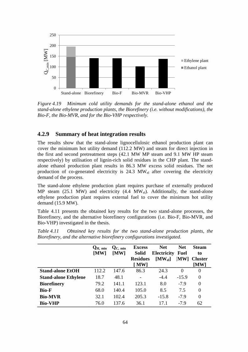
64


stand-alone ethylene production plants, the Biorefinery (i.e. without modifications), the

Bio-F, the Bio-MVR, and for the Bio-VHP respectively.

4.2.9 Summary of heat integration results

The results show that the stand-alone lignocellulosic ethanol production plant can

cover the minimum hot utility demand (112.2 MW) and steam for direct injection in

the first and second pretreatment steps (42.1 MW MP steam and 9.1 MW HP steam

respectively) by utilisation of lignin-rich solid residues in the CHP plant. The stand-

alone ethanol production plant results in 86.3 MW excess solid residues. The net

production of co-generated electricity is 24.3 MWel after covering the electricity

demand of the process.

The stand-alone ethylene production plant requires purchase of externally produced

MP steam (25.1 MW) and electricity (4.4 MWel). Additionally, the stand-alone

ethylene production plant requires external fuel to cover the minimum hot utility

demand (15.9 MW).

Table 4.11 presents the obtained key results for the two stand-alone processes, the

Biorefinery, and the alternative biorefinery configurations (i.e. Bio-F, Bio-MVR, and

Bio-VHP) investigated in the thesis.

Table 4.11 Obtained key results for the two stand-alone production plants, the

Biorefinery, and the alternative biorefinery configurations investigated.

QH, min

[MW]

QC, min

[MW]

Excess

Solid

Residues

[ MW]

Net

Electricity

[MWel]

Net

Fuel

[MW]

Steam

to

Cluster

[MW]

Stand-alone EtOH 112.2 147.6 86.3 24.3 0 0

Stand-alone Ethylene 18.7 48.1 - -4.4 -15.9 0

Biorefinery 79.2 141.1 123.1 8.0 -7.9 0

Bio-F 68.0 140.4 105.0 8.5 7.5 0

Bio-MVR 32.1 102.4 205.3 -15.8 -7.9 0

Bio-VHP 76.0 137.6 36.1 17.1 -7.9 62

0

50

100

150

200

250

Stand-alone Biorefinery Bio-F Bio-MVR Bio-VHP

QC

,min

[M

W]

Ethylene plant

Ethanol plant

65

The results from the background/foreground analysis, see Section 4.2.3, indicate that

heat integration of the two stand-alone processes have a potential to reduce the

minimum hot and cold utility demand by 31% and 21% respectively. The reduction is

mainly due to the waste heat recovery in the stand-alone ethylene production plant.

Combining the two stand-alone processes into a biorefinery (delivering ethanol directly

to the ethylene production plant in gas phase) the minimum hot and cold utility

demand can be further reduced. The results show that the minimum hot and cold utility

demand is reduced by 40% and 28% respectively by integrating the two stand-alone

processes into a biorefinery. The results also show that the minimum hot and cold

utility demand of the biorefinery can be further reduced (i.e. by 59% and 27%

respectively) by introducing a MVR on the rectifier reflux. Compared with the two

stand-alone processes the MVR implementation corresponds to a minimum hot utility

reduction of 75%.

The results indicate that the stand-alone lignocellulosic ethanol production results in

sufficient amount of excess solid residues to cover the MP steam requirement in the

stand-alone ethylene production plant. Additionally the electricity demand of the stand-

alone ethylene production plant can be covered with co-generated electricity produced

in the CHP plant. The results show that the resulting lignin-rich solid residues in the

ethanol production additionally has the potential to cover the ethylene reactor furnace

by flue gas integration or producing 62 MW VHP steam for covering the heat deficit in

the chemical cluster. Both integration opportunities result in excess solid residues.

Furthermore the ethylene by-products are not utilised in the Bio-F configuration and

can thus be sold, introducing an additional revenue source, however this is enabled at

the expense of excess solid residues. The introduction of a MVR significantly increases

the amount of excess solid residues (due to the reduction in minimum hot utility

demand).

All process configurations investigated except for the stand-alone ethylene production

and Bio-MVR result in a net electricity production, allowing export to the grid.

4.3 Economic evaluation

4.3.1 Total capital cost estimation

4.3.1.1 Stand-alone lignocellulosic ethanol and stand-alone ethanol dehydration

to ethylene production

The total capital costs for the stand-alone lignocellulosic ethanol and the stand-alone

ethanol dehydration to ethylene production plants are estimated at 394 million € and

91 million € respectively. The capital cost for the stand-alone lignocellulosic ethanol

production is estimated by calculating the capital cost for each equipment individually

(see Appendix I and J) as discussed in Section 3.5.1. The total capital cost for the

stand-alone ethanol dehydration to ethylene production is estimated with an average

total capital cost between 61 and 122 million € gathered from literature (Jones, et al.,

2010). The total capital costs for the two stand-alone plants are presented in

Table 4.12.

66

Table 4.12 Total capital cost for the two stand-alone production plants.

Total capital cost

[Million €]

Stand-alone EtOH 393.9

Stand-alone Ethylene 91.1

4.3.1.2 Biorefinery – Ethylene production from lignocellulosic feedstock

The total capital cost for the biorefinery is estimated by calculating the capital cost for

each equipment individually (see Appendix I and Appendix J), as discussed in Section

3.5.1. Parameters affecting the biorefinery capital cost between the different

configurations are:

- CHP plant size

- MVR system implementation

- Separate furnace

The total capital cost of the ethylene production plant is fixed at 91 million € in all

biorefinery capital cost estimations expect in Bio-F. The elimination of the furnace

reduces the total capital cost for the ethylene plant by 1 million € (Gavin, et al., 2008).

Table 4.13 presents the estimated total capital costs for the different biorefinery

configurations.

Table 4.13 Total capital cost estimations for the biorefinery configurations

investigated.

Total Capital Cost

[Million €]

Biorefinery 474.7

Bio-F 479.9

Bio-MVR 450.7

Bio-VHP 496.9

Investigating the impact flue gas integration with the ethylene reactors (i.e. eliminating

the separate furnace) has on the total capital cost, a comparison between the

Biorefinery and Bio-F is conducted. The results indicate that the elimination of the

separate furnace, by integrating the ethylene reactors with the CHP plant flue gases,

increases the total capital cost of the biorefinery. The integration results in an increased

solid fuel load to the CHP plant, increasing the CHP plant size, hence the total capital

cost is increased.

The introduction of a MVR results in the addition of one unit (i.e. a compressor). The

introduction of a MVR system in the biorefinery significantly reduces the minimum

hot utility demand, and consequently reduces the CHP plant size. As seen in

Table 4.13 the Bio-MVR results in comparatively lower capital cost.

Investigating the influence VHP steam delivery to the chemical cluster has on the total

capital cost, a comparison between the Biorefinery and Bio-VHP is conducted. As

67

expected the CHP plant size increases due to the increased steam production, and

thereby the total capital cost of the biorefinery increases.

The results show that the CHP plant size has a great impact on the total capital cost

(approximately 20%). As can been seen in Table 4.13 the Bio-VHP and the Bio-MVR

obtains the highest and lowest total capital costs respectively.

4.3.2 Annual operating cost estimation



In the annual operating costs for the stand-alone lignocellulosic ethanol and the stand-

alone ethanol dehydration to ethylene production plants all the expenses for the two

stand-alone production plants are included, see Section 3.5.2. Table 4.14 presents

assumed prices in the estimation. Note that no income is taken into consideration in the

annual operating cost estimation, but it is treated in a separate section, see

Section 4.3.3. See Appendix K for exchange rates used.

Table 4.14 Assumed prices for raw materials, energy demands, and labour used in

the annual operating cost estimation.

The annual operating costs for the stand-alone lignocellulosic ethanol production and

the stand-alone ethanol dehydration to ethylene production plant are estimated at

193 million € and 201 million € respectively, see Table 4.15. It should be noted that the

stand-alone ethanol production plant is energy self-sufficient, while the stand-alone

ethylene production plant requires purchase of steam, fuel, and electricity. The annual

operating costs are estimated at full production of the two stand-alone production

plants respectively.

7 Assumed efficiency of 80%

Price Reference

Spruce 121 €/tonnedry (Karlsson, 2009)

Yeast 18 €/tonne (Fornell, 2010)

Enzyme 115 €/tonne (Fornell, 2010)

Sulphuric Acid 35 €/tonne (ICIS)

Process Water (Fresh water) 1.15 €/tonne (Spetz, 2011)

Purchase of Ethanol 497 €/tonne (ICIS)

Steam 41.1 €/MWh Based on natural gas price7

Fuel (Natural Gas) 32.9 €/MWh (Göteborgs Energi)

Purchased Electricity Price 68.9 €/MWh (Spetz, 2011)

Shift operator 31.8 €/h

Supervision 47.7 €/h

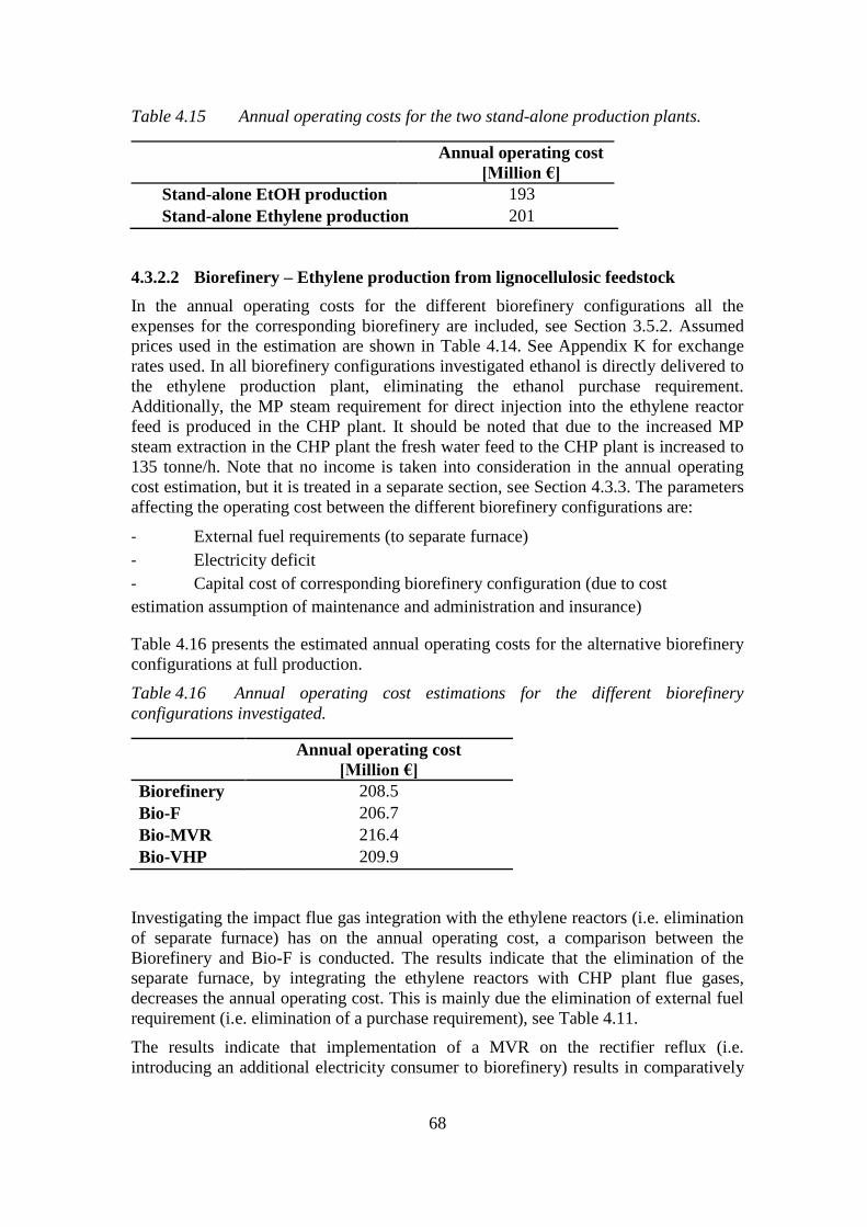
68

Table 4.15 Annual operating costs for the two stand-alone production plants.

Annual operating cost

[Million €]

Stand-alone EtOH production 193

Stand-alone Ethylene production 201


In the annual operating costs for the different biorefinery configurations all the

expenses for the corresponding biorefinery are included, see Section 3.5.2. Assumed

prices used in the estimation are shown in Table 4.14. See Appendix K for exchange

rates used. In all biorefinery configurations investigated ethanol is directly delivered to

the ethylene production plant, eliminating the ethanol purchase requirement.

Additionally, the MP steam requirement for direct injection into the ethylene reactor

feed is produced in the CHP plant. It should be noted that due to the increased MP

steam extraction in the CHP plant the fresh water feed to the CHP plant is increased to

135 tonne/h. Note that no income is taken into consideration in the annual operating

cost estimation, but it is treated in a separate section, see Section 4.3.3. The parameters

affecting the operating cost between the different biorefinery configurations are:

- External fuel requirements (to separate furnace)

- Electricity deficit

- Capital cost of corresponding biorefinery configuration (due to cost

estimation assumption of maintenance and administration and insurance)

Table 4.16 presents the estimated annual operating costs for the alternative biorefinery

configurations at full production.

Table 4.16 Annual operating cost estimations for the different biorefinery

configurations investigated.

Annual operating cost

[Million €]

Biorefinery 208.5

Bio-F 206.7

Bio-MVR 216.4

Bio-VHP 209.9

Investigating the impact flue gas integration with the ethylene reactors (i.e. elimination

of separate furnace) has on the annual operating cost, a comparison between the

Biorefinery and Bio-F is conducted. The results indicate that the elimination of the

separate furnace, by integrating the ethylene reactors with CHP plant flue gases,

decreases the annual operating cost. This is mainly due the elimination of external fuel

requirement (i.e. elimination of a purchase requirement), see Table 4.11.

The results indicate that implementation of a MVR on the rectifier reflux (i.e.

introducing an additional electricity consumer to biorefinery) results in comparatively

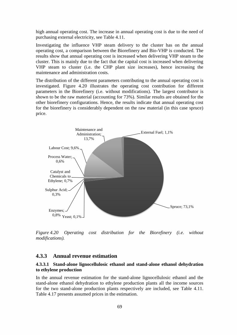
69

high annual operating cost. The increase in annual operating cost is due to the need of

purchasing external electricity, see Table 4.11.

Investigating the influence VHP steam delivery to the cluster has on the annual

operating cost, a comparison between the Biorefinery and Bio-VHP is conducted. The

results show that annual operating cost is increased when delivering VHP steam to the

cluster. This is mainly due to the fact that the capital cost is increased when delivering

VHP steam to cluster (i.e. the CHP plant size increases), hence increasing the

maintenance and administration costs.

The distribution of the different parameters contributing to the annual operating cost is

investigated. Figure 4.20 illustrates the operating cost contribution for different

parameters in the Biorefinery (i.e. without modifications). The largest contributor is

shown to be the raw material (accounting for 73%). Similar results are obtained for the

other biorefinery configurations. Hence, the results indicate that annual operating cost

for the biorefinery is considerably dependent on the raw material (in this case spruce)

price.

Figure 4.20 Operating cost distribution for the Biorefinery (i.e. without

modifications).

4.3.3 Annual revenue estimation



In the annual revenue estimation for the stand-alone lignocellulosic ethanol and the

stand-alone ethanol dehydration to ethylene production plants all the income sources

for the two stand-alone production plants respectively are included, see Table 4.11.

Table 4.17 presents assumed prices in the estimation.

Spruce; 73,1%

Yeast; 0,1%

Enzymes;

0,8%

Sulphur Acid;

0,3%

Catalyst and

Chemicals to

Ethylene; 0,7%

Process Water;

0,6%

Labour Cost; 9,6%

Maintenance and

Administration;

13,7%

External Fuel; 1,1%

70

Table 4.17 Assumed prices for the co-products used in the revenue estimation.

The income sources taken into consideration in the stand-alone lignocellulosic ethanol

production plant are ethanol, excess solid residues, and net electricity production. The

selling price of ethanol is estimated from the minimum production cost, see Section

4.3.4.1. The only income source taken into consideration in the stand-alone ethanol

dehydration to ethylene production is the ethylene product. The selling price of

ethylene is estimated from the minimum production cost, see Section 4.3.4.1.

The annual sales incomes for the stand-alone lignocellulosic ethanol production and

the stand-alone ethanol dehydration to ethylene production plant at full production are

estimated at 242 million € and 212 million € respectively, see Table 4.18.

Table 4.18 Annual revenue estimations for the two stand-alone production plants.

Annual revenue

[Million €]

Stand-alone EtOH production 242

Stand-alone Ethylene production 212


In the annual revenue estimation for the different biorefinery configurations all the

income sources for the corresponding biorefinery are included; ethylene (the same for

all biorefinery configurations), excess solid residues, net electricity production,

ethylene column by-products (for Bio-F), and VHP steam (for Bio-VHP), see

Table 4.11. The selling price of ethylene is estimated from the minimum production

cost, see Section 4.3.4.2. Table 4.17 presents assumed prices in the estimation.

Table 4.19 presents the annual sales incomes for the different biorefinery

configurations at full production.

Table 4.19 Annual revenue estimations for the different biorefinery configurations

investigated.

Annual revenue

[Million €]

Biorefinery 258

Bio-F 257

Bio-MVR 264

Bio-VHP 262

8 Assumed efficiency of 80%

Price Reference

Solid-residues (Pellets) 34.9 €/MWh (Karlsson, 2009)

Steam 41.1 €/MWh Based on natural gas price8

Electricity 91.9 €/MWh (Spetz, 2011)

By-products (Ethylene Column) 32.9 €/MWh Based on natural gas price

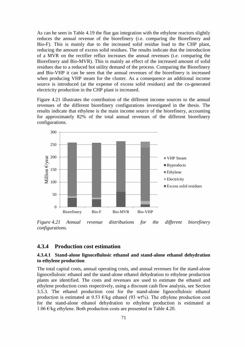
71

As can be seen in Table 4.19 the flue gas integration with the ethylene reactors slightly

reduces the annual revenue of the biorefinery (i.e. comparing the Biorefinery and

Bio-F). This is mainly due to the increased solid residue load to the CHP plant,

reducing the amount of excess solid residues. The results indicate that the introduciion

of a MVR on the rectifier reflux increases the annual revenues (i.e. comparing the

Biorefinery and Bio-MVR). This is mainly an effect of the increased amount of solid

residues due to a reduced hot utility demand of the process. Comparing the Biorefinery

and Bio-VHP it can be seen that the annual revenues of the biorefinery is increased

when producing VHP steam for the cluster. As a consequence an additional income

source is introduced (at the expense of excess solid residues) and the co-generated

electricity production in the CHP plant is increased.

Figure 4.21 illustrates the contribution of the different income sources to the annual

revenues of the different biorefinery configurations investigated in the thesis. The

results indicate that ethylene is the main income source of the biorefinery, accounting

for approximately 82% of the total annual revenues of the different biorefinery

configurations.

Figure 4.21 Annual revenue distributions for the different biorefinery

configurations.

4.3.4 Production cost estimation



The total capital costs, annual operating costs, and annual revenues for the stand-alone

lignocellulosic ethanol and the stand-alone ethanol dehydration to ethylene production

plants are identified. The costs and revenues are used to estimate the ethanol and

ethylene production costs respectively, using a discount cash flow analysis, see Section

3.5.3. The ethanol production cost for the stand-alone lignocellulosic ethanol

production is estimated at 0.53 €/kg ethanol (93 wt%). The ethylene production cost

for the stand-alone ethanol dehydration to ethylene production is estimated at

1.06 €/kg ethylene. Both production costs are presented in Table 4.20.

0

50

100

150

200

250

300

Biorefinery Bio-F Bio-MVR Bio-VHP

Mil

lion €

/yea

r

VHP Steam

Byproducts

Ethylene

Electricity

Excess solid residues

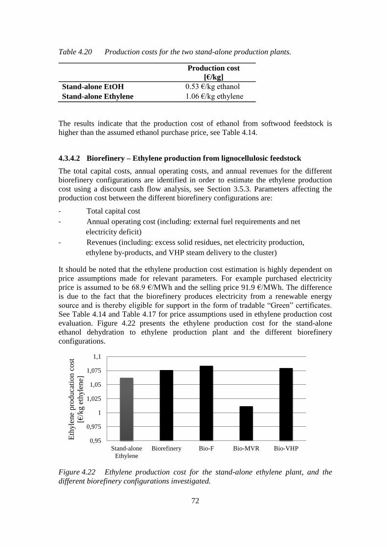
72

Table 4.20 Production costs for the two stand-alone production plants.

Production cost

[€/kg]

Stand-alone EtOH 0.53 €/kg ethanol

Stand-alone Ethylene 1.06 €/kg ethylene

The results indicate that the production cost of ethanol from softwood feedstock is

higher than the assumed ethanol purchase price, see Table 4.14.


The total capital costs, annual operating costs, and annual revenues for the different

biorefinery configurations are identified in order to estimate the ethylene production

cost using a discount cash flow analysis, see Section 3.5.3. Parameters affecting the

production cost between the different biorefinery configurations are:

- Total capital cost

- Annual operating cost (including: external fuel requirements and net

electricity deficit)

- Revenues (including: excess solid residues, net electricity production,

ethylene by-products, and VHP steam delivery to the cluster)

It should be noted that the ethylene production cost estimation is highly dependent on

price assumptions made for relevant parameters. For example purchased electricity

price is assumed to be 68.9 €/MWh and the selling price 91.9 €/MWh. The difference

is due to the fact that the biorefinery produces electricity from a renewable energy

source and is thereby eligible for support in the form of tradable “Green” certificates.

See Table 4.14 and Table 4.17 for price assumptions used in ethylene production cost

evaluation. Figure 4.22 presents the ethylene production cost for the stand-alone

ethanol dehydration to ethylene production plant and the different biorefinery

configurations.

Figure 4.22 Ethylene production cost for the stand-alone ethylene plant, and the

different biorefinery configurations investigated.

0,95

0,975

1

1,025

1,05

1,075

1,1

Stand-alone

Ethylene

Biorefinery Bio-F Bio-MVR Bio-VHP

Eth

yle

ne

pro

duca

tion c

ost

[€/k

g e

thyle

ne]

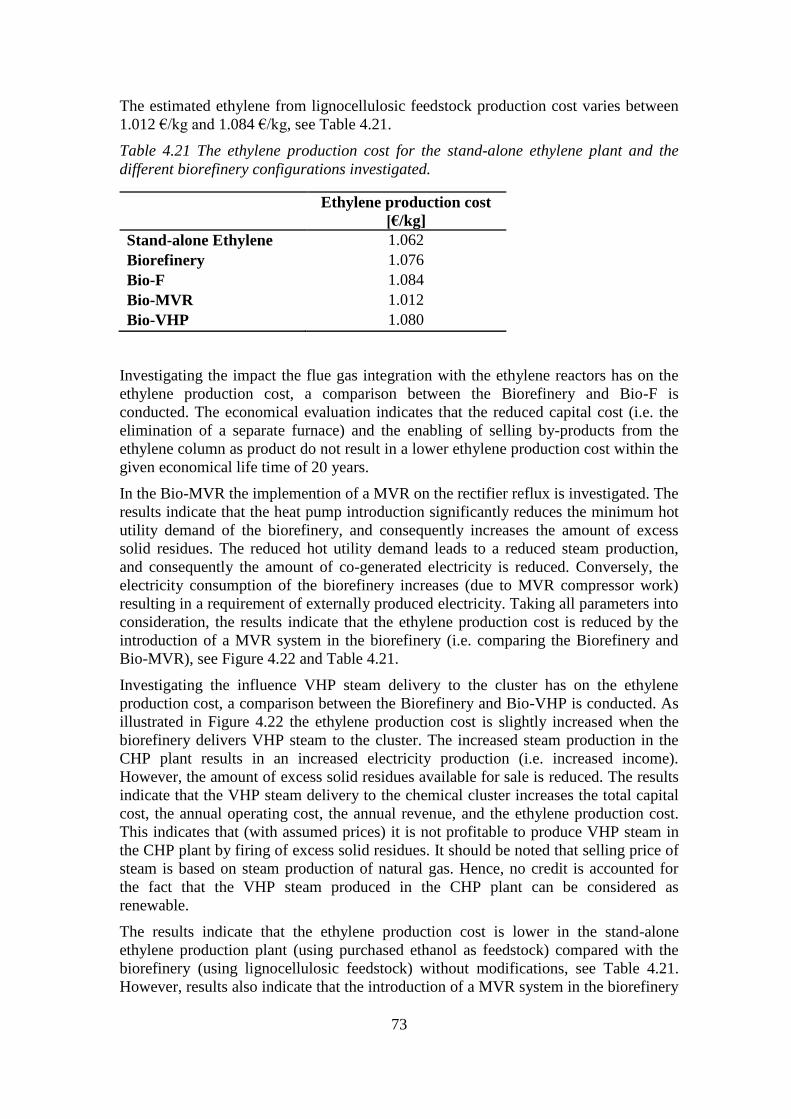
73

The estimated ethylene from lignocellulosic feedstock production cost varies between

1.012 €/kg and 1.084 €/kg, see Table 4.21.

Table 4.21 The ethylene production cost for the stand-alone ethylene plant and the

different biorefinery configurations investigated.

Ethylene production cost

[€/kg]

Stand-alone Ethylene 1.062

Biorefinery 1.076

Bio-F 1.084

Bio-MVR 1.012

Bio-VHP 1.080

Investigating the impact the flue gas integration with the ethylene reactors has on the

ethylene production cost, a comparison between the Biorefinery and Bio-F is

conducted. The economical evaluation indicates that the reduced capital cost (i.e. the

elimination of a separate furnace) and the enabling of selling by-products from the

ethylene column as product do not result in a lower ethylene production cost within the

given economical life time of 20 years.

In the Bio-MVR the implemention of a MVR on the rectifier reflux is investigated. The

results indicate that the heat pump introduction significantly reduces the minimum hot

utility demand of the biorefinery, and consequently increases the amount of excess

solid residues. The reduced hot utility demand leads to a reduced steam production,

and consequently the amount of co-generated electricity is reduced. Conversely, the

electricity consumption of the biorefinery increases (due to MVR compressor work)

resulting in a requirement of externally produced electricity. Taking all parameters into

consideration, the results indicate that the ethylene production cost is reduced by the

introduction of a MVR system in the biorefinery (i.e. comparing the Biorefinery and

Bio-MVR), see Figure 4.22 and Table 4.21.

Investigating the influence VHP steam delivery to the cluster has on the ethylene

production cost, a comparison between the Biorefinery and Bio-VHP is conducted. As

illustrated in Figure 4.22 the ethylene production cost is slightly increased when the

biorefinery delivers VHP steam to the cluster. The increased steam production in the

CHP plant results in an increased electricity production (i.e. increased income).

However, the amount of excess solid residues available for sale is reduced. The results

indicate that the VHP steam delivery to the chemical cluster increases the total capital

cost, the annual operating cost, the annual revenue, and the ethylene production cost.

This indicates that (with assumed prices) it is not profitable to produce VHP steam in

the CHP plant by firing of excess solid residues. It should be noted that selling price of

steam is based on steam production of natural gas. Hence, no credit is accounted for

the fact that the VHP steam produced in the CHP plant can be considered as

renewable.

The results indicate that the ethylene production cost is lower in the stand-alone

ethylene production plant (using purchased ethanol as feedstock) compared with the

biorefinery (using lignocellulosic feedstock) without modifications, see Table 4.21.

However, results also indicate that the introduction of a MVR system in the biorefinery

74

(Bio-MVR) can reduce the ethylene production cost (mainly due to substantial

reduction in minimum hot utility demand) of the biorefinery. A 59% minimum hot

utility demand reduction in the biorefinery corresponds to an ethylene production cost

reduction of 6% (i.e. comparing the Biorefinery and Bio-MVR). This is due to the fact

that the cost of raw material purchase is the largest contributor (i.e. 73%) to the annual

operating cost of the biorefinery. Additionally, ethylene is the main income source (i.e.

approximately 82%) of the biorefinery. The results indicate that the ethylene

production using softwood feedstock in a biorefinery can be more profitable than

purchasing ethanol (produced in Europe) to a stand-alone ethylene production plant, if

introducing a MVR system in the biorefinery.

75

5 Conclusion

The results show that 277.6 kg ethanol per tonne dry wood can be produced in the

stand-alone lignocellulosic ethanol plant. The results indicate that the process can

cover the minimum hot utility (112 MW) and steam for direct injection into process

streams (42 MW and 9 MW) by firing of lignin-rich solid residues in a CHP plant. The

stand-alone ethanol production results in excess of solid residues (86 MW) and

electricity (24 MWel).

The results show that 0.57 kg ethylene per kg ethanol can be produced in the stand-

alone ethanol dehydration to ethylene plant. The results indicate that the process

requires external fuel (16 MW) to cover the minimum hot utility demand after

implementation of a FEHX and firing of by-products (7.5 MW). Additionally,

electricity (4 MWel) and steam for direct injection (25 MW) must be produced

externally.

The results indicate that 158.2 kg ethylene per tonne dy wood can be obtained

combining the stand-alone lignocellulosic ethanol and the stand-alone ethanol

dehydration to ethylene production into a biorefinery producing ethylene from

lignocellulosic feedstock. The integration of the two stand-alone processes into a

biorefinery results in a minimum hot and cold utility demand of 79 MW and 141 MW

respectively, which corresponds to 40% and 28% reduction respectively. The reduction

is mainly due to reuse of excess heat available in the ethylene production plant. By

introducing a MVR on the rectifier reflux (Bio-MVR) the minimum hot utility demand

of the biorefinery can be further reduced by 59%, corresponding to a 75% reduction

compared with the two stand-alone processes.

The results indicate that the amount of lignin-rich solid residues generated by the

ethanol production process is sufficient to cover the minimum hot utility, steam for

direct injection, and electricity demand of the biorefinery. Moreover, the results show

that the excess solid residues can eliminate the external fuel requirement of the

catalytic ethylene reactors by integration of flue gases. Alternatively, the excess solid

residues can be utilised in the CHP plant producing VHP (41 bar) steam to cover the

heat deficit (i.e. 62 MW after site wide energy efficiency measures) in the cluster.

The results indicate that the ethylene production cost in the biorefinery without

modifications is higher compared with the stand-alone ethylene production using

purchased ethanol as feedstock. Additionally, the results indicate that it is not

profitable to use excess solid residues in a CHP plant to eliminate the separate furnace.

The results also show that it is not profitable to produce VHP steam for the chemical

cluster by firing solid residues. However, the results indicate that the introduction of a

MVR heat pump on the rectifier reflux in the biorefinery reduces the ethylene

production cost by 6% (i.e. from 1.076 to 1.012 €/kg ethylene). The substantial energy

savings achieved by the introduction of a MVR in the biorefinery also results in a

lower ethylene production cost compared with the stand-alone ethylene production

plant. Hence, the results indicate that the ethylene production in a biorefinery using

softwood feedstock can be more profitable than in a stand-alone ethylene production

plant purchasing ethanol (produced in Europe), if introducing a MVR system in the

biorefinery. Figure 5.1 illustrates an overview of main material and energy streams in

Bio-MVR.

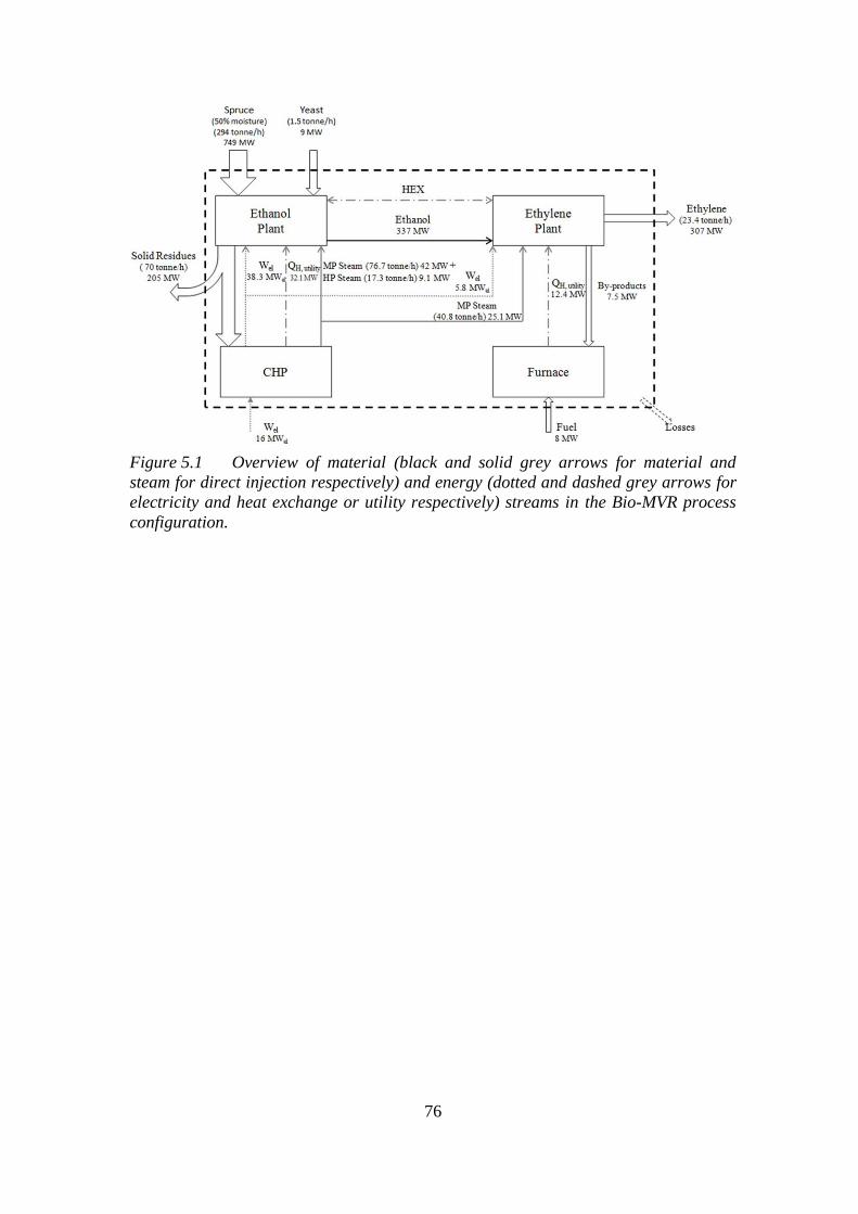
76



electricity and heat exchange or utility respectively) streams in the Bio-MVR process

configuration.

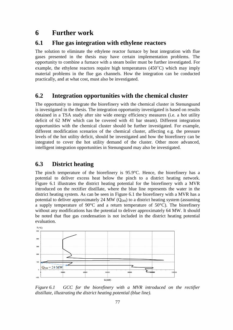
77

6 Further work

6.1 Flue gas integration with ethylene reactors

The solution to eliminate the ethylene reactor furnace by heat integration with flue

gases presented in the thesis may have certain implementation problems. The

opportunity to combine a furnace with a steam boiler must be further investigated. For

example, the ethylene reactors require high temperatures (450°C) which may imply

material problems in the flue gas channels. How the integration can be conducted

practically, and at what cost, must also be investigated.

6.2 Integration opportunities with the chemical cluster

The opportunity to integrate the biorefinery with the chemical cluster in Stenungsund

is investigated in the thesis. The integration opportunity investigated is based on results

obtained in a TSA study after site wide energy efficiency measures (i.e. a hot utility

deficit of 62 MW which can be covered with 41 bar steam). Different integration

opportunities with the chemical cluster should be further investigated. For example,

different modification scenarios of the chemical cluster, affecting e.g. the pressure

levels of the hot utility deficit, should be investigated and how the biorefinery can be

integrated to cover the hot utility demand of the cluster. Other more advanced,

intelligent integration opportunities in Stenungsund may also be investigated.

6.3 District heating

The pinch temperature of the biorefinery is 95.9°C. Hence, the biorefinery has a

potential to deliver excess heat below the pinch to a district heating network.

Figure 6.1 illustrates the district heating potential for the biorefinery with a MVR

introduced on the rectifier distillate, where the blue line represents the water in the

district heating system. As can be seen in Figure 6.1 the biorefinery with a MVR has a

potential to deliver approximately 24 MW (QDH) to a district heating system (assuming

a supply temperature of 90°C and a return temperature of 50°C). The biorefinery

without any modifications has the potential to deliver approximately 64 MW. It should

be noted that flue gas condensation is not included in the district heating potential

evaluation.

Figure 6.1 GCC for the biorefinery with a MVR introduced on the rectifier

distillate, illustrating the district heating potential (blue line).

78

Currently there is no demand for expanding the existing district heating network in

Stenungsund. If developing new technologies enabling district heat delivery on longer

distances the district heating potential of the biorefinery could be further investigated.

The district heating could bring in an extra income to the biorefinery.

6.4 Sustainable ethylene?

Furthermore, a thorough investigation is required to decide whether the produced

ethylene can be considered to be sustainable. A more detailed analysis needs to be

conducted to decide which is the most sustainable: a biorefinery in Stenungsund

producing ethylene from lignocellulosic feedstock or a stand-alone ethylene production

plant in Stenungsund purchasing ethanol feedstock. Parameters to be investigated

include differences in CO2 emissions, electricity production/consumption, and climate

impact. The availability of sufficient amounts of lignocellulosic raw material in the

area needs to be investigated when studying the alternative of introducing a biorefinery

in Stenungsund. One question to ask may be if the produced ethylene can be

considered to be sustainable if the raw material (in this case ethanol) is transported

from far distances (e.g. from South America) and the electricity demand is covered by

electricity produced from non-renewable resources in Europe?

79

7 References

Aden A. [et al.] Lignocellulosic biomass to ethanol process design and economics

utilizing co-current dilute acid prehydrolysis and enzymatic hydrolysis for corn stover

[Report] : Technical Report / National Renewable Energy Laboratory. - 2002.

Alkasrawi M., Galbe M. and Zacchi G. Recirculation of process streams in suel

ethanol production from softwood based on simultaneous saccharification and

fermentation [Journal] // Applied Biochemistry and Biotechnology. - 2002. - Vols. 98-

100. - pp. 849-861.

Borealis AB Annual Report [Report]. - Stenungsund : [s.n.], 2010.

Borealis AB Miljörapport [Report]. - Stenungsund : [s.n.], 2007.

Braskem Green Plastic [Online]. - Braskem, 2010. - Oct 25, 2010. -

http://www.braskem.com/plasticoverde/EN_HOME.html.

Cardona-Alzate C.A. and Sánchez Toro O.J. Energy consumption analysis of

integrated flowsheets for production of fuel ethanol from lignocellulosic biomass

[Journal] // Energy. - 2006. - 31. - pp. 2447-2459.

Carvalheiro F., Duarte L.C. and Gírío F.M. Hemicellulose biorefineries: A review

on biomass pretreatments [Journal] // Journal of Scientific Industrial Research. -

2008. - Vol. 67. - pp. 849-864.

Chematur AB Ethanol Derivatives [Online]. - Oct 29, 2010. - www.chematur.se.

Eklund R., Galbe M. and Zacchi G. The influence of SO2 and H2SO4 impregnation

of willow prior to steam explosion [Journal] // Bioresource Engineering. - 1995. - 52. -

pp. 225-229.

Eriksson G. and Kjellström B. Assessment of combined heat and power (CHP)

integrated with wood-based ethanol production [Journal] // Applied Energy. - 2010. -

Vol. 87. - pp. 3632-3641.

Fornell R. Energy efficiency measures in a kraft pulp mill converted to a biorefinery

producing ethanol [Report] : Lic. Eng / Department of Heat and Power Technology ;

Chalmers University of Technology. - Göteborg : [s.n.], 2010.

Franzén C.J. Interview with Associate Professor Carl Johan Franzén from Industrial

Biotechnology Department, Chalmers University of Technology [Interview]. - Nov 18,

2010.

Galbe M. [et al.] Process engineering economics of bioethanol production [Journal] //

Advanced Biochemical Engineering/Biotechnology. - 2007. - 108. - pp. 303-327.

Galbe M. and Zacchi G. A review of a production of ethanol from softwood

[Journal] // Applied Microbiology Biotechnology. - 2002. - 59. - pp. 618-628.

Gavin P., Towler R. and Sinnott K. Chemical Engineering Design: Principles,

Practice and Economics of Plant and Process Design [Book]. - 2008.

Gellerstedt G. [et al.] The Ljungberg Textbook Wood Chemistry [Book]. - 2008.

Göteborgs Energi Göteborg Energi Naturgasavtal [Online]. - 02 25, 2011. -

http://www.goteborgenergi.se/Foretag/Gas/Erbjudanden_och_priser/Naturgashandel/R

orligt_naturgaspris.

80

Gregg D.J., Boussaid A. and Saddler J.N. Techno-economic evaluations of a generic

wood-to-ethanol process: effect of increased cellulose yields and enzyme recycle

[Journal] // Bioresource Technology. - 1998. - 63. - pp. 7-12.

Grous W.R., Converse A.O. and Grethlein H.E. Effect of steam explosion

pretreatment on pore size and enzymatic hydrolysis of poplar [Journal] // Enzyme and

Microbial Technology. - 1986. - 5 : Vol. 8. - pp. 274-280.

Hackl R. and Perret S. Power production with Organic Rankine Cycle technology

utilizing waste heat from a cracker and three polyethylene units [Report] : MSc

Thesis. - Göteborg : [s.n.], 2009.

Hackl R., Andersson E. and Harvey S. Targeting for energy efficiency and improved

energy collaboration between different companies using total site analysis [Journal] //

Chemical Engineering Transactions. - 2010. - Vol. 21. - pp. 301-306.

Hamelinck C.N., van Hooijdonk G. and Faaij A.P.C. Ethanol from lignocellulosic

biomass: techno-economic performance in short-, middle- and long-term [Journal] //

Biomass and Bioenergy. - 2005. - 28. - pp. 384-410.

Harvey S. Industrial Energy Systems [Book]. - [s.l.] : Divsion of Heat and Power

Technology, Chalmers University of Technology, 2009.

Holtzapple M.T. [et al.] Pretreatment of lignocellulosic municipal solid waste by

ammonia fiber explosion (AFEX) [Journal] // Applied Biochemistry and

Biotechnology. - 1992. - 1 : Vols. 34-35. - pp. 5-12.

Huang H. Microbial ethanol, its polymer polyethylene, and applications [Journal] //

Plastics from Bacteria: Natural Functions and Applications. - 2010. - Vol. 14.

ICIS ICIS pricing Ethanol (Europe) [Online]. - ICIS. - 02 20, 2011. -

www.icispricing.com/il_shared/Samples/SubPage108.asp.

Jones M.J., Maughon B.R. and Kresge C.T. Alternative feedstocks for olefin

production: What role will ethanol play? [Journal] // Oil Gas Magazine. - 2010. - 1.

Karlsson S. Swedish statistical yearbook of foresty [Report]. - 2009.

Kemp I.C. Pinch Analysis and Process Integration: A User Guide on Process

Integration for the Efficient Use of Energy [Book]. - Oxford : Butterworth-Heinemann,

Elsevier Ltd, 2007.

Kochar N.K., Merims R. and Padia A.S. Ethylene from ethanol [Journal] //

Chemical Engineering Progress, AlChE. - 1981. - 6. - pp. 66-70, 77.

Larsson M., Galbe M. and Zacchi G. Recirculation of process water in the

production of ethanol from softwood [Journal] // Bioresource Technology. - 1997. -

60. - pp. 143-151.

Larsson S. [et al.] The generation of fermentation inhibitors during dilute acid

hydrolysis of softwood [Journal] // Enzyme and Microbial Technology. - 1999. - Vol.

24. - pp. 151-159.

Macki K.L., Brownell H.H. and West K.L. Effect of sulphur dioxide and sulphuric

acid on steam explosion of aspenwood [Journal] // Journal of Wood Chemistry and

Technology. - 1985. - 3 : Vol. 5. - pp. 405-425.

81

Monavari S., Galbe M. and Zacchi G. The influence of solid/liquid separation

techniques on the sugar yield in two-step dilute acid hydrolysis of softwood followed

by enzymatic hydrolysis [Journal] // Biotechnology for Biofuels. - 2009. - 2 : Vol. 6.

Morschbaker A. Bio-ethanol based ethylene [Journal] // Macromolecular Science. -

2009. - 49. - pp. 79-84.

Mosier N. [et al.] Features of promising technologies for pretreatment of

lignocellulosic biomass [Journal] // Bioresource Technology. - 2005. - Vol. 96. - pp.

673-686.

National Renewable Energy Labratory Corn Stover to Ethanol [Aspen Plus Backup

File]. - 2004.

Nguyen Q.A. [et al.] Two-stage dilute-acid pretreatment of softwoods [Journal] //

Applied Biochemistry and Biotechnology. - 2000. - Vols. 84-86.

Olsson L. and Hahn-Hägerdal B. Fermentative performance of bacteria and yeasts in

lignocellulose hydrolysates [Journal] // Process Biochemistry. - 1993. - 4 : Vol. 28. -

pp. 249-257.

Pan X. [et al.] Biorefining of softwoods using ethanol organosolv pulping: Preliminary

evaluation of process streams for manufacture of fuel-grade ethanol and co-products

[Journal] // Biotechnology and Bioengineering. - 2005. - 90. - pp. 473-481.

Sassner P. and Zacchi G. Integration options for high energy efficiency and improved

economics in a wood-to-ethanol process [Journal] // Biotechnology for Biofuels. -

2008. - 1 : Vol. 4.

Sassner P. Lignocellulosic ethanol production based on steam pretreatment and SSF

[Report] : PhD Thesis. - Department of Chemical Engineering : Lund University, 2007.

Sassner P., Galbe M. and Zacchi G. Techno-economic evaluation of bioethanol

production from three different lignocellulosic materials [Journal] // Biomass and

Bioenergy. - 2008. - 32. - pp. 422-430.

Schnelle K.B. and Brown C.A. Air Pollution Control Technology Handbook

[Book]. - 2002.

Söderström J. [et al.] Two-step steam pretreatment of softwood by dilute H2SO4

impregnation for ethanol production [Journal] // Biomass and Bioenergy. - 2003. - 24. -

pp. 475-486.

Söderström J. [et al.] Two-step steam pretreatment of softwood with SO2

impregnation for ethanol production [Journal] // Applied Biochemistry and

Biotechnology. - 2002. - Vols. 98-100.

Söderström J., Galbe M. and Zacchi G. Separate versus simultaneous

saccharification and fermentation of two-step steam pretreated softwood for ethanol

production [Journal] // Journal of Wood Chemistry and Technology. - 2005. - 3 : Vol.

25. - pp. 187-202.

Spetz R. Energy Specialist at Borealis AB, personal communication [Interview]. -

2011.

Statistiska Centralbyrån [Online]. - Feb 20, 2011. - www.scb.se.

82

Stauffer John E. and Kranich Wilmer L. Kinetics of the catalytic dehydration of

primary alcohols [Journal] // I&EC Fundamentals. - 1962. - 2 : Vol. 1.

Stenberg K. [et al.] Optimisation of steam pretreatment of SO2-impregnated mixed

softwoods for ethanol production [Journal] // J. Chem. Technol. Biotechnol.. - 1998b. -

71. - pp. 299-308.

Stenberg K. [et al.] Recycling of process streams in ethanol production from

softwoods based on enzymatic hydrolysis [Journal] // Applied Biochemistry and

Biotechnology. - 1998a. - Vols. 70-72.

Sun Y. and Cheng J. Hydrolysis of lignocellulosic materials for ethanol production: A

review [Journal] // Bioresource Technology. - 2002. - 1. - pp. 1-11.

Tengborg C. [et al.] Comparison of SO2 and H2SO4 impregnation of softwood prior

to steam pretreatment on ethanol production [Journal] // Applied Biochemistry and

Biotechonology. - 1998. - Vols. 70-72.

Tengborg C., Galbe M. and Zacchi G. Reduced inhibition of enzymatic hydrolysis of

steam-pretreated softwood [Journal] // Enzyme and Microbial Technology. - 2001. -

28. - pp. 835-844.

Valladares Barrocas H.V. and Lacerda A.I. Process for production of ethylene from

ethyl alcohol [Patent]. - Nov 29, 2007.

Valladares Barrocas H.V., de Castro M. da Silva J.B. and Coutinho de Assis R. Process for preparing ethene [Patent]. - United States of America, Nov 4, 1980.

von Sivers M. and Zacchi G. A techno-economical comparison of three processes for

the production of ethanol from pine [Journal] // Bioresource Technology. - 1995. - 51. -

pp. 43-52.

von Sivers M. and Zacchi G. Ethanol from lignocellulosics: A review of the economy

[Journal]. - [s.l.] : Bioresource Technology, 1996. - 56. - pp. 131-140.

Wingren A. [et al.] Process considerations and economic evaluation of two-step steam

pretreatment for production of fuel ethanol from softwood [Journal] // Biotechonology

Programme. - 2004. - 5 : Vol. 20. - pp. 1421-1429.

Wingren A. Ethanol from softwood, techno-economic evaluation for development of

the enzymatic process [Report] : PhD Thesis. - Department of Chemical Engineering :

Lund University, 2005.

Wingren A., Galbe M. and Zacchi G. Energy considerations for a SSF-based

softwood ethanol plant [Journal] // Bioresource Technology. - 2008. - 7 : Vol. 99. - pp.

2121-2131.

Wingren A., Galbe M. and Zacchi G. Techno-economic evaluation of producing

ethanol from softwood: Comparison of SSF and SHF and identification of bottlenecks

[Journal] // Biotechnology Prog.. - 2003. - 4 : Vol. 19. - pp. 1109-1117.

Winter O. and Eng M.T. Make ethylene from ethanol [Journal] // Hydrocarbon

Processing. - Nov 1976.

Wooley R.J. and Putsche V. Development of an Aspen Plus physical property

database for biofuels components [Report] / National Renewable Energy Laboratory. -

1996.

83

x-rates Exchange Rates [Online]. - 03 02, 2011. - www.x-rates.com.

Zhu J.Y. and Pan X.J. Woody biomass pretreatment for cellulosic ethanol

production: Technology and energy consumption evaluation [Journal] // Bioresource

Technology. - 2010. - 101.

85

Appendix A: Alternative pretreatment methods

Hemicellulose and cellulose in lignocellulosic raw material can be made accessible for

the downstream hydrolysis through addition of a base catalyst, i.e. undergo alkali

pretreatment. The addition of a base catalyst, such as sodium-, calcium-, potassium

hydroxide, or ammonia, affects the lignin association with hemicellulose and cellulose.

The alkaline pretreatment achieves high efficiencies for agricultural residue and some

hardwood species (Galbe, et al., 2002). The achieved effect is highly dependent on the

lignin content of the feedstock. The efficiency decreases with increasing lignin content

(Galbe, et al., 2002; Sun, et al., 2002; Holtzapple, et al., 1992).

The alkali pretreatment method is followed by some environmental concerns. The

process requires high concentrations of salts, as a consequence a costly chemical

recovery step is necessary. Also additional expenses concerning wastewater treatment

and solid residue deposition may occur, e.g. due to incorporated salts into the biomass

(Mosier, et al., 2005). However, one advantage with the process is the mild operating

conditions (Carvalheiro, et al., 2008).

A combination of alkaline pretreatment and steam explosion can also be applied to

lignocellulosic raw material, i.e. Ammonia Fiber Explosion (AFEX). The pretreatment

method obtains very high sugar yields for both hemicellulose and cellulose (over 90%

hydrolysis) for low lignin-containing agricultural residues. The method shows

moderate success for hardwood. Furthermore, it is not an efficient pretreatment method

handling softwood feedstock (Sun, et al., 2002). Some drawbacks with the AFEX

pretreatment are the safety issues concerning handling ammonia and the need for

chemical recovery. However, when employing the AFEX pretreatment method no

sugar degradation occurs, leading to a higher overall sugar recovery and no inhibition

in the downstream hydrolysis or fermentation steps. (Mosier, et al., 2005)

The recalcitrance of biomass can also be overcome by the organosolv pretreatment, i.e.

the addition of an organic solvent and an inorganic catalyst. Examples of organic

solvents are ethanol, methanol, and acetone. Common catalysts used are HCl and

H2SO4. The conversion of cellulose in downstream hydrolysis step has been shown to

be successful for large amount of different feedstocks. Some studies suggest that this

also applies to hardwood and softwood (Zhu, et al., 2010). However, in order to avoid

inhibition in the subsequent hydrolysis and fermentation step the solvent needs to be

removed (Sun, et al., 2002). The resulting solid residue, i.e. lignin, obtains very high

purity and quality when employing the organosolv pretreatment (Pan, et al., 2005).

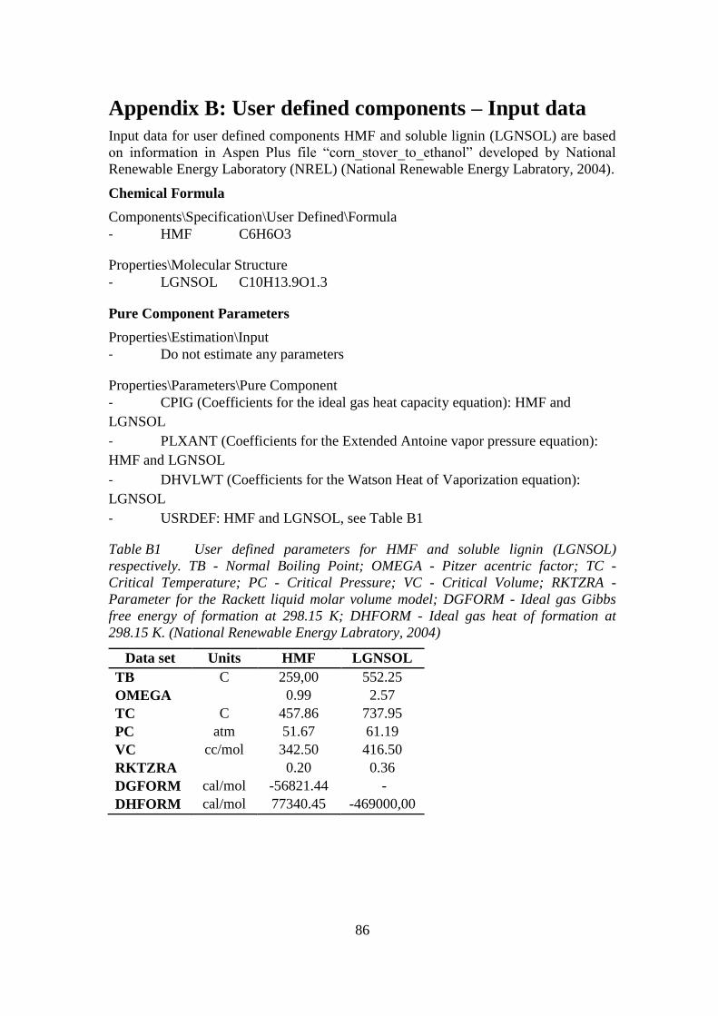
86

Appendix B: User defined components – Input data

Input data for user defined components HMF and soluble lignin (LGNSOL) are based

on information in Aspen Plus file “corn_stover_to_ethanol” developed by National

Renewable Energy Laboratory (NREL) (National Renewable Energy Labratory, 2004).

Chemical Formula

Components\Specification\User Defined\Formula

- HMF C6H6O3

Properties\Molecular Structure

- LGNSOL C10H13.9O1.3

Pure Component Parameters

Properties\Estimation\Input

- Do not estimate any parameters

Properties\Parameters\Pure Component

- CPIG (Coefficients for the ideal gas heat capacity equation): HMF and

LGNSOL

- PLXANT (Coefficients for the Extended Antoine vapor pressure equation):

HMF and LGNSOL

- DHVLWT (Coefficients for the Watson Heat of Vaporization equation):

LGNSOL

- USRDEF: HMF and LGNSOL, see Table B1

Table B1 User defined parameters for HMF and soluble lignin (LGNSOL)

respectively. TB - Normal Boiling Point; OMEGA - Pitzer acentric factor; TC -

Critical Temperature; PC - Critical Pressure; VC - Critical Volume; RKTZRA -

Parameter for the Rackett liquid molar volume model; DGFORM - Ideal gas Gibbs

free energy of formation at 298.15 K; DHFORM - Ideal gas heat of formation at

298.15 K. (National Renewable Energy Labratory, 2004)

Data set Units HMF LGNSOL

TB C 259,00 552.25

OMEGA 0.99 2.57

TC C 457.86 737.95

PC atm 51.67 61.19

VC cc/mol 342.50 416.50

RKTZRA 0.20 0.36

DGFORM cal/mol -56821.44 -

DHFORM cal/mol 77340.45 -469000,00

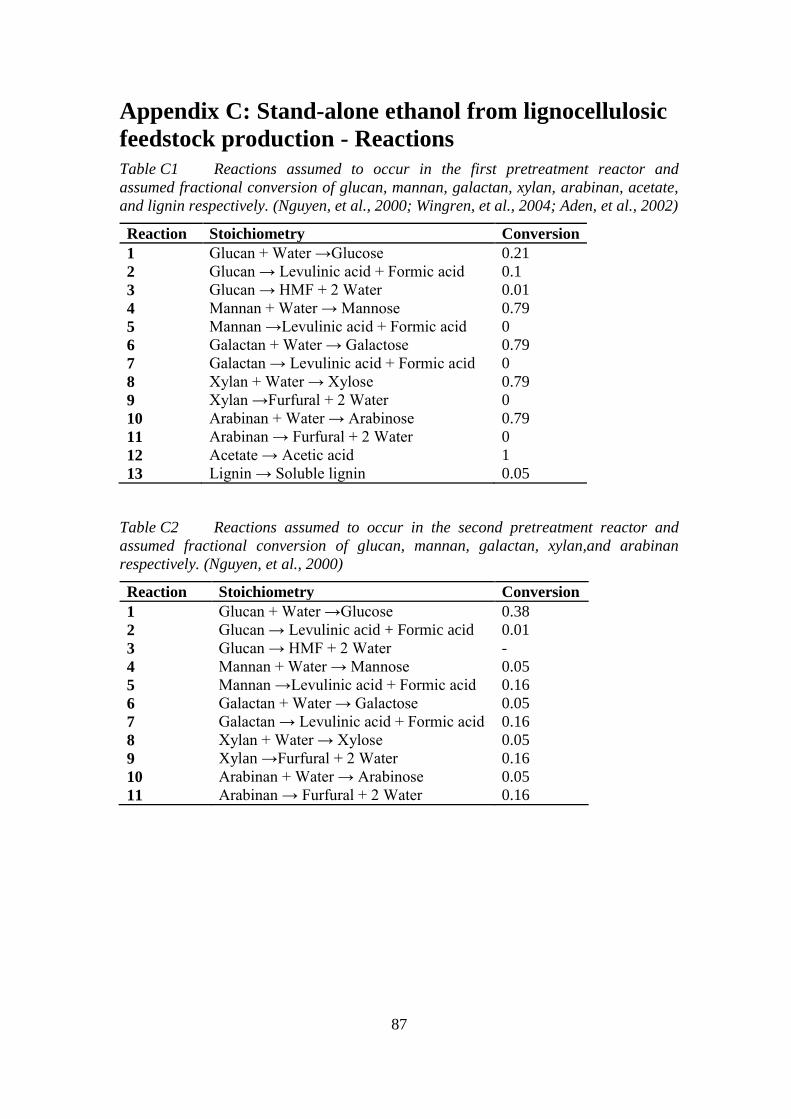
87

Appendix C: Stand-alone ethanol from lignocellulosic

feedstock production - Reactions

Table C1 Reactions assumed to occur in the first pretreatment reactor and

assumed fractional conversion of glucan, mannan, galactan, xylan, arabinan, acetate,

and lignin respectively. (Nguyen, et al., 2000; Wingren, et al., 2004; Aden, et al., 2002)

Reaction Stoichiometry Conversion

1 Glucan + Water →Glucose 0.21

2 Glucan → Levulinic acid + Formic acid 0.1

3 Glucan → HMF + 2 Water 0.01

4 Mannan + Water → Mannose 0.79

5 Mannan →Levulinic acid + Formic acid 0

6 Galactan + Water → Galactose 0.79

7 Galactan → Levulinic acid + Formic acid 0

8 Xylan + Water → Xylose 0.79

9 Xylan →Furfural + 2 Water 0

10 Arabinan + Water → Arabinose 0.79

11 Arabinan → Furfural + 2 Water 0

12 Acetate → Acetic acid 1

13 Lignin → Soluble lignin 0.05

Table C2 Reactions assumed to occur in the second pretreatment reactor and

assumed fractional conversion of glucan, mannan, galactan, xylan,and arabinan

respectively. (Nguyen, et al., 2000)


1 Glucan + Water →Glucose 0.38

2 Glucan → Levulinic acid + Formic acid 0.01

3 Glucan → HMF + 2 Water -

4 Mannan + Water → Mannose 0.05

5 Mannan →Levulinic acid + Formic acid 0.16

6 Galactan + Water → Galactose 0.05

7 Galactan → Levulinic acid + Formic acid 0.16

8 Xylan + Water → Xylose 0.05

9 Xylan →Furfural + 2 Water 0.16

10 Arabinan + Water → Arabinose 0.05

11 Arabinan → Furfural + 2 Water 0.16

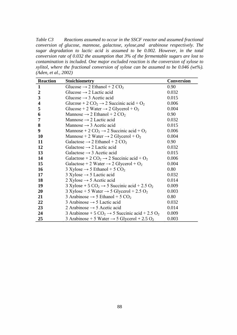
88

Table C3 Reactions assumed to occur in the SSCF reactor and assumed fractional

conversion of glucose, mannose, galactose, xylose,and arabinose respectively. The

sugar degradation to lactic acid is assumed to be 0.002. However, in the total

conversion rate of 0.032 the assumption that 3% of the fermentable sugars are lost to

contamination is included. One major excluded reaction is the conversion of xylose to

xylitol, where the fractional conversion of xylose can be assumed to be 0.046 (wt%).

(Aden, et al., 2002)


1 Glucose → 2 Ethanol + 2 CO2 0.90

2 Glucose → 2 Lactic acid 0.032

3 Glucose → 3 Acetic acid 0.015

4 Glucose + 2 CO2 → 2 Succinic acid + O2 0.006

5 Glucose + 2 Water → 2 Glycerol + O2 0.004

6 Mannose → 2 Ethanol + 2 CO2 0.90

7 Mannose → 2 Lactic acid 0.032

8 Mannose → 3 Acetic acid 0.015

9 Mannose + 2 CO2 → 2 Succinic acid + O2 0.006

10 Mannose + 2 Water → 2 Glycerol + O2 0.004

11 Galactose → 2 Ethanol + 2 CO2 0.90

12 Galactose → 2 Lactic acid 0.032

13 Galactose → 3 Acetic acid 0.015

14 Galactose + 2 CO2 → 2 Succinic acid + O2 0.006

15 Galactose + 2 Water → 2 Glycerol + O2 0.004

16 3 Xylose → 5 Ethanol + 5 CO2 0.80

17 3 Xylose → 5 Lactic acid 0.032

18 2 Xylose → 5 Acetic acid 0.014

19 3 Xylose + 5 CO2 → 5 Succinic acid + 2.5 O2 0.009

20 3 Xylose + 5 Water → 5 Glycerol + 2.5 O2 0.003

21 3 Arabinose → 5 Ethanol + 5 CO2 0.80

22 3 Arabinose → 5 Lactic acid 0.032

23 2 Arabinose → 5 Acetic acid 0.014

24 3 Arabinose + 5 CO2 → 5 Succinic acid + 2.5 O2 0.009

25 3 Arabinose + 5 Water → 5 Glycerol + 2.5 O2 0.003

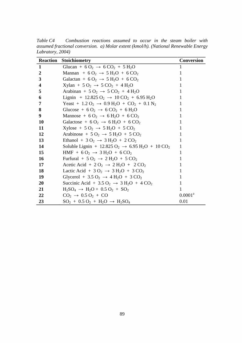
89

Table C4 Combustion reactions assumed to occur in the steam boiler with

assumed fractional conversion. a) Molar extent (kmol/h). (National Renewable Energy

Labratory, 2004)


1 Glucan + 6 O2 → 6 CO2 + 5 H2O 1

2 Mannan + 6 O2 → 5 H2O + 6 CO2 1

3 Galactan + 6 O2 → 5 H2O + 6 CO2 1

4 Xylan + 5 O2 → 5 CO2 + 4 H2O 1

5 Arabinan + 5 O2 → 5 CO2 + 4 H2O 1

6 Lignin + 12.825 O2 → 10 CO2 + 6.95 H2O 1

7 Yeast + 1.2 O2 → 0.9 H2O + CO2 + 0.1 N2 1

8 Glucose + 6 O2 → 6 CO2 + 6 H2O 1

9 Mannose + 6 O2 → 6 H2O + 6 CO2 1

10 Galactose + 6 O2 → 6 H2O + 6 CO2 1

11 Xylose + 5 O2 → 5 H2O + 5 CO2 1

12 Arabinose + 5 O2 → 5 H2O + 5 CO2 1

13 Ethanol + 3 O2 → 3 H2O + 2 CO2 1

14 Soluble Lignin + 12.825 O2 → 6.95 H2O + 10 CO2 1

15 HMF + 6 O2 → 3 H2O + 6 CO2 1

16 Furfural + 5 O2 → 2 H2O + 5 CO2 1

17 Acetic Acid + 2 O2 → 2 H2O + 2 CO2 1

18 Lactic Acid + 3 O2 → 3 H2O + 3 CO2 1

19 Glycerol + 3.5 O2 → 4 H2O + 3 CO2 1

20 Succinic Acid + 3.5 O2 → 3 H2O + 4 CO2 1

21 H2SO4 → H2O + 0.5 O2 + SO2 1

22 CO2 → 0.5 O2 + CO 0.0001a

23 SO2 + 0.5 O2 + H2O → H2SO4 0.01

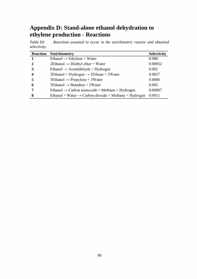
90

Appendix D: Stand-alone ethanol dehydration to

ethylene production - Reactions

Table D1 Reactions assumed to occur in the stoichimetric reactor and obtained

selectivity.

Reaction Stoichiometry Selectivity

1 Ethanol → Ethylene + Water 0.988

2 2Ethanol → Diethyl ether + Water 0.00052

3 Ethanol → Acetaldehyde + Hydrogen 0.002

4 2Ethanol + Hydrogen → 2Ethane + 2Water 0.0027

5 3Ethanol → Propylene + 3Water 0.0006

6 2Ethanol → Butadien + 2Water 0.005

7 Ethanol → Carbon monoxide + Methane + Hydrogen 0.00007

8 Ethanol + Water → Carbon dioxide + Methane + Hydrogen 0.0011

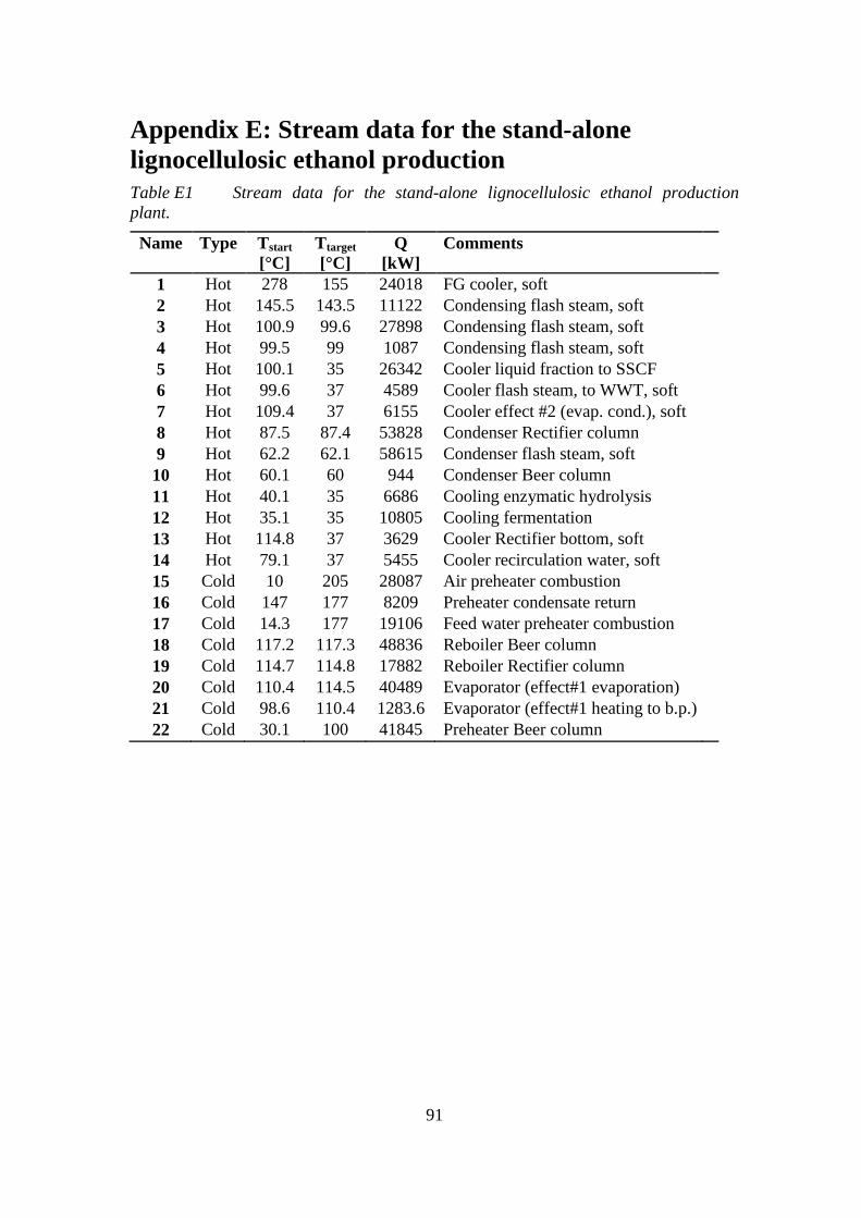
91

Appendix E: Stream data for the stand-alone

lignocellulosic ethanol production

Table E1 Stream data for the stand-alone lignocellulosic ethanol production

plant.

Name Type Tstart

[°C]

Ttarget

[°C]

Q

[kW]

Comments

1 Hot 278 155 24018 FG cooler, soft 2 Hot 145.5 143.5 11122 Condensing flash steam, soft 3 Hot 100.9 99.6 27898 Condensing flash steam, soft 4 Hot 99.5 99 1087 Condensing flash steam, soft 5 Hot 100.1 35 26342 Cooler liquid fraction to SSCF 6 Hot 99.6 37 4589 Cooler flash steam, to WWT, soft 7 Hot 109.4 37 6155 Cooler effect #2 (evap. cond.), soft 8 Hot 87.5 87.4 53828 Condenser Rectifier column 9 Hot 62.2 62.1 58615 Condenser flash steam, soft 10 Hot 60.1 60 944 Condenser Beer column 11 Hot 40.1 35 6686 Cooling enzymatic hydrolysis 12 Hot 35.1 35 10805 Cooling fermentation 13 Hot 114.8 37 3629 Cooler Rectifier bottom, soft 14 Hot 79.1 37 5455 Cooler recirculation water, soft 15 Cold 10 205 28087 Air preheater combustion 16 Cold 147 177 8209 Preheater condensate return 17 Cold 14.3 177 19106 Feed water preheater combustion 18 Cold 117.2 117.3 48836 Reboiler Beer column 19 Cold 114.7 114.8 17882 Reboiler Rectifier column 20 Cold 110.4 114.5 40489 Evaporator (effect#1 evaporation) 21 Cold 98.6 110.4 1283.6 Evaporator (effect#1 heating to b.p.) 22 Cold 30.1 100 41845 Preheater Beer column

92

Appendix F: Stream data for the stand-alone ethanol

dehydration to ethylene production

Table F1 Stream data for the stand-alone ethanol dehydration to ethylene

production plant.

Name Type Tstart

[°C]

Ttarget

[°C]

Q

[kW]

Comments

1 Hot 428 172 13251.4 Reactor effluent #1

2 Hot 172 156.77 25128.0 Reactor effluent #2

3 Hot 156.7 140.4 7699.8 Reactor effluent #3


5 Hot 114.9 84 4151.6 Reactor effluent #5

6 Hot 132.9 38 1844.7 Midcooler#1 Compressor

7 Hot 128 38 1287.9 Midcooler#2 Compressor


9 Hot 61.2 20 1939.4 Cooler Quench tower

10 Hot 56.5 15 532.1 Cooler before dryer

11 Hot 15 -17.2 2337.3 Precooler C2 splitter

12 Hot -25 -25.1 7578.7 Condenser C2 splitter

13 Cold 169 450 21244.2 Furnace #1

14 Cold 385.6 450 3562.0 Furnace #2

15 Cold 386.9 450 3476.0 Furnace #3

16 Cold 389 450 3345.0 Furnace #4

17 Cold 11.2 11.3 6091.2 Reboiler C2 splitter

18 Cold -21.4 -21.3 1379.5 Reboiler Stripper

19 Cold 25 135 4274.4 Preheat Ethanol feed

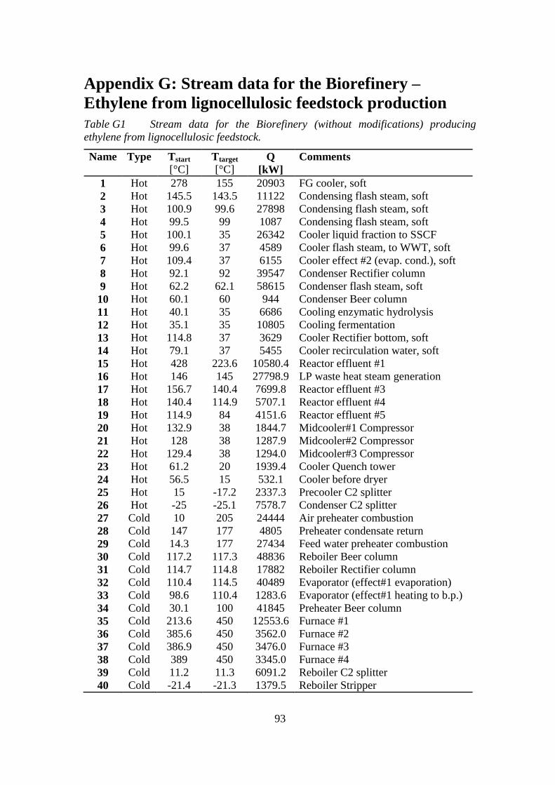
93

Appendix G: Stream data for the Biorefinery –

Ethylene from lignocellulosic feedstock production

Table G1 Stream data for the Biorefinery (without modifications) producing

ethylene from lignocellulosic feedstock.

Name Type Tstart

[°C] Ttarget

[°C] Q

[kW]

Comments

1 Hot 278 155 20903 FG cooler, soft

2 Hot 145.5 143.5 11122 Condensing flash steam, soft


4 Hot 99.5 99 1087 Condensing flash steam, soft

5 Hot 100.1 35 26342 Cooler liquid fraction to SSCF

6 Hot 99.6 37 4589 Cooler flash steam, to WWT, soft

7 Hot 109.4 37 6155 Cooler effect #2 (evap. cond.), soft

8 Hot 92.1 92 39547 Condenser Rectifier column

9 Hot 62.2 62.1 58615 Condenser flash steam, soft

10 Hot 60.1 60 944 Condenser Beer column

11 Hot 40.1 35 6686 Cooling enzymatic hydrolysis

12 Hot 35.1 35 10805 Cooling fermentation

13 Hot 114.8 37 3629 Cooler Rectifier bottom, soft

14 Hot 79.1 37 5455 Cooler recirculation water, soft


16 Hot 146 145 27798.9 LP waste heat steam generation











27 Cold 10 205 24444 Air preheater combustion

28 Cold 147 177 4805 Preheater condensate return

29 Cold 14.3 177 27434 Feed water preheater combustion

30 Cold 117.2 117.3 48836 Reboiler Beer column

31 Cold 114.7 114.8 17882 Reboiler Rectifier column

32 Cold 110.4 114.5 40489 Evaporator (effect#1 evaporation)

33 Cold 98.6 110.4 1283.6 Evaporator (effect#1 heating to b.p.)

34 Cold 30.1 100 41845 Preheater Beer column

35 Cold 213.6 450 12553.6 Furnace #1

36 Cold 385.6 450 3562.0 Furnace #2

37 Cold 386.9 450 3476.0 Furnace #3

38 Cold 389 450 3345.0 Furnace #4



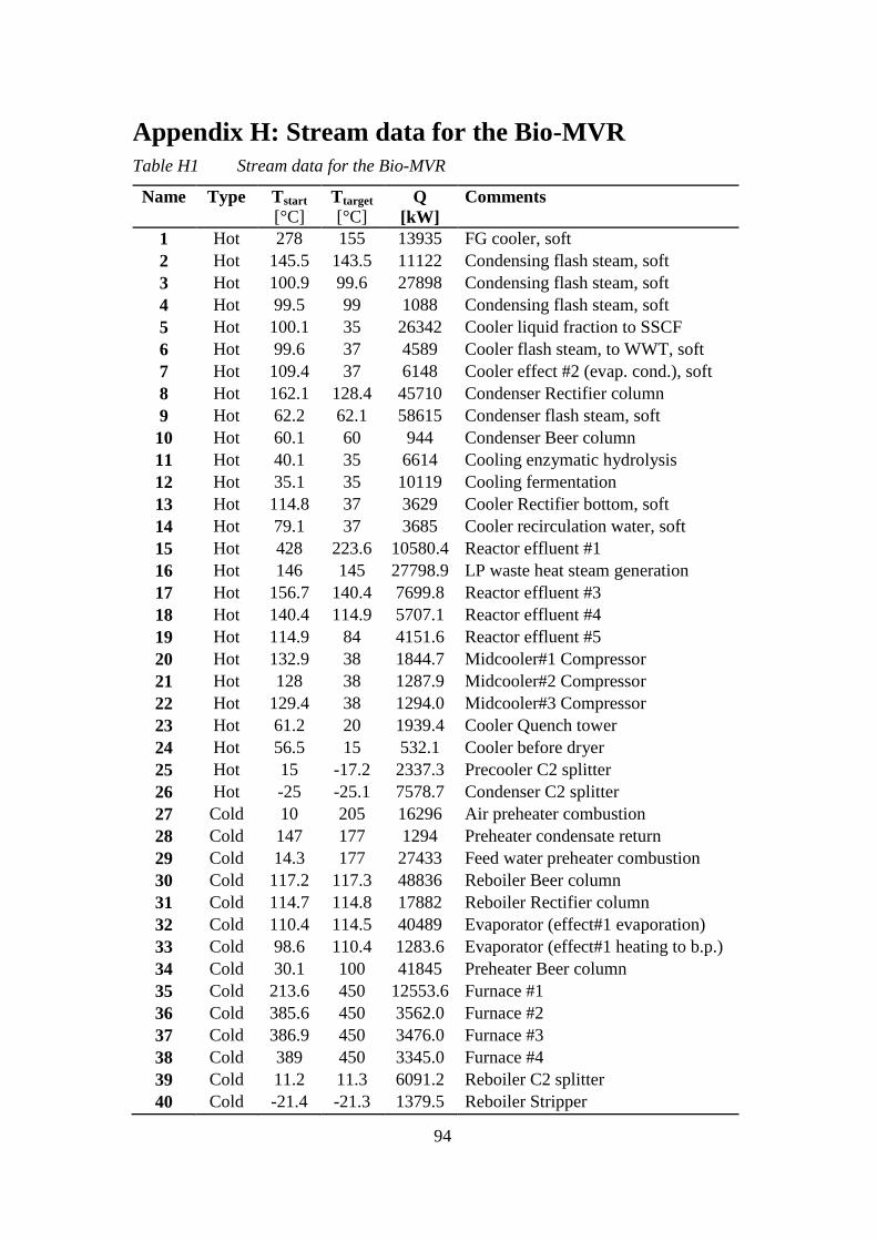
94

Appendix H: Stream data for the Bio-MVR

Table H1 Stream data for the Bio-MVR

Name Type Tstart

[°C] Ttarget

[°C] Q

[kW]

Comments

1 Hot 278 155 13935 FG cooler, soft



4 Hot 99.5 99 1088 Condensing flash steam, soft

5 Hot 100.1 35 26342 Cooler liquid fraction to SSCF

6 Hot 99.6 37 4589 Cooler flash steam, to WWT, soft

7 Hot 109.4 37 6148 Cooler effect #2 (evap. cond.), soft

8 Hot 162.1 128.4 45710 Condenser Rectifier column

9 Hot 62.2 62.1 58615 Condenser flash steam, soft

10 Hot 60.1 60 944 Condenser Beer column

11 Hot 40.1 35 6614 Cooling enzymatic hydrolysis

12 Hot 35.1 35 10119 Cooling fermentation

13 Hot 114.8 37 3629 Cooler Rectifier bottom, soft

14 Hot 79.1 37 3685 Cooler recirculation water, soft


16 Hot 146 145 27798.9 LP waste heat steam generation











27 Cold 10 205 16296 Air preheater combustion

28 Cold 147 177 1294 Preheater condensate return

29 Cold 14.3 177 27433 Feed water preheater combustion

30 Cold 117.2 117.3 48836 Reboiler Beer column

31 Cold 114.7 114.8 17882 Reboiler Rectifier column

32 Cold 110.4 114.5 40489 Evaporator (effect#1 evaporation)

33 Cold 98.6 110.4 1283.6 Evaporator (effect#1 heating to b.p.)

34 Cold 30.1 100 41845 Preheater Beer column

35 Cold 213.6 450 12553.6 Furnace #1

36 Cold 385.6 450 3562.0 Furnace #2

37 Cold 386.9 450 3476.0 Furnace #3

38 Cold 389 450 3345.0 Furnace #4



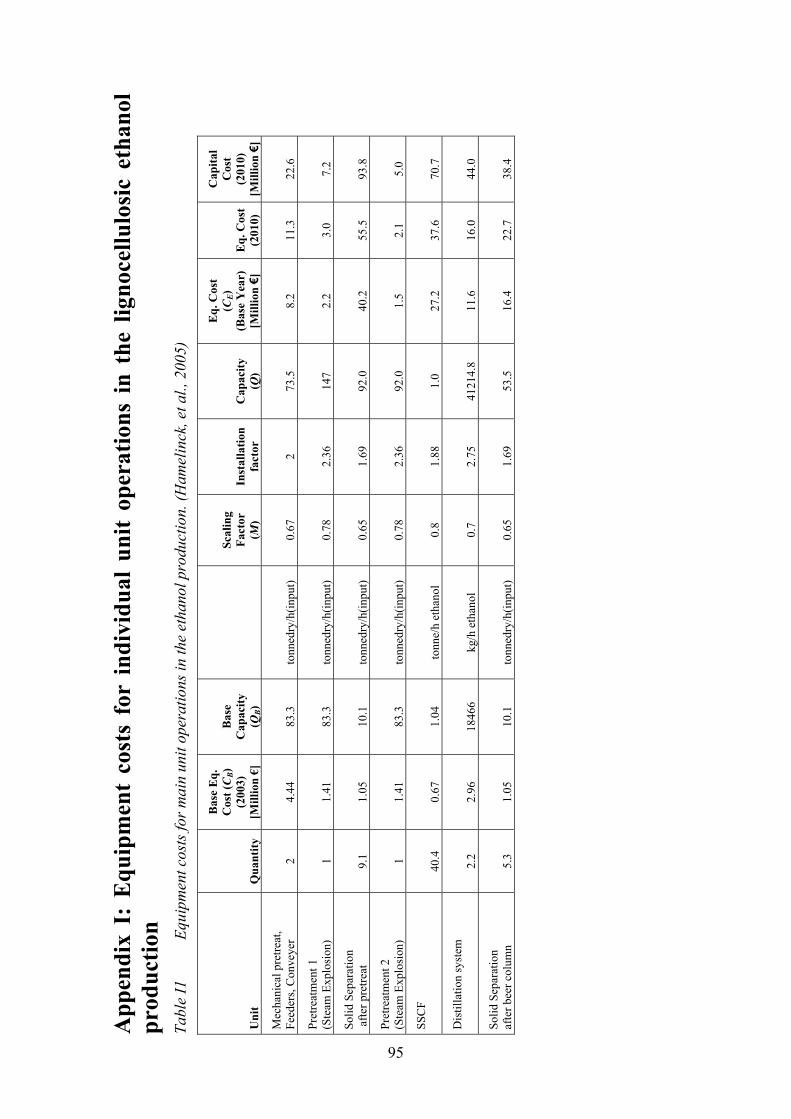
Ap

pen

dix

I:

Eq

uip

men

t co

sts

for

ind

ivid

ual

un

it o

per

atio

ns

in t

he

lign

ocel

lulo

sic

eth

anol

p

rod

uct

ion

T

able

I1

E

quip

men

t cos

ts fo

r m

ain

unit

ope

rati

ons

in th

e et

hano

l pro

duct

ion.

(H

amel

inck

, et a

l., 2

005)

Un

it

Qu

anti

ty

Bas

e E

q.

Cos

t (C

B)

(200

3)

[Mil

lion

€]

Bas

e C

apac

ity

(QB)

Sca

lin

g F

acto

r (M

) In

stal

lati

on

fact

or

Cap

acit

y (Q

)

Eq.

Cos

t

(CE)

(Bas

e Y

ear)

[M

illio

n €

] E

q. C

ost

(201

0)

Cap

ital

C

ost

(201

0)

[Mil

lion

€]

Mec

hani

cal p

retr

eat,

Fee

ders

, Con

veye

r 2

4.44

83

.3

tonn

edry

/h(i

nput

) 0.

67

2 73

.5

8.2

11.3

22

.6

Pre

trea

tmen

t 1

(Ste

am E

xplo

sion

) 1

1.41

83

.3

tonn

edry

/h(i

nput

) 0.

78

2.36

14

7 2.

2 3.

0 7.

2

Sol

id S

epar

atio

n a

fter

pre

trea

t 9.

1 1.

05

10.1

to

nned

ry/h

(inp

ut)

0.65

1.

69

92.0

40

.2

55.5

93

.8

Pre

trea

tmen

t 2

(Ste

am E

xplo

sion

) 1

1.41

83

.3

tonn

edry

/h(i

nput

) 0.

78

2.36

92

.0

1.5

2.1

5.0

SS

CF

40.4

0.

67

1.04

to

nne/

h et

hano

l 0.

8 1.

88

1.0

27.2

37

.6

70.7

Dis

till

atio

n sy

stem

2.2

2.96

18

466

kg/h

eth

anol

0.

7 2.

75

4121

4.8

11.6

16

.0

44.0

Sol

id S

epar

atio

n af

ter

beer

col

umn

5.3

1.05

10

.1

tonn

edry

/h(i

nput

) 0.

65

1.69

53

.5

16.4

22

.7

38.4

95

Tab

le I

2

Equ

ipm

ent c

osts

for

mai

n pu

mps

in th

e et

hano

l pro

duct

ion.

(A

den,

et a

l., 2

002)

Un

it

Qu

anti

ty

Bas

e E

q.

Cos

t (C

B)

(200

3)

[Mil

lion

€]

Bas

e C

apac

ity

(QB)

Sca

lin

g F

acto

r (M

) In

stal

lati

on

fact

or

Cap

acit

y (Q

)

Eq

. Cos

t (C

E)

(Bas

e Y

ear)

[M

illio

n €

]

Eq

. C

ost

(201

0)

Cap

ital

Cos

t (2

010)

[M

illio

n €

]

Pum

p 1

1 10

600

1710

56

kg/h

0.

79

2.8

2154

03

0.00

9 0.

013

0.03

7

Pum

p 2,

Sul

phur

ic A

cid

1 48

00

3289

kg

/h

0.79

2.

8 14

70

0.00

2 0.

003

0.00

5

Pum

p 3,

Sul

phur

ic A

cid

1 48

00

3289

kg

/h

0.79

2.

8 73

5 0.

001

0.00

2 0.

003

Pum

p 4

1 10

600

1710

56

kg/h

0.

79

2.8

9080

5 0.

005

0.00

7 0.

013

Pum

p 5

1 10

600

1710

56

kg/h

0.

79

2.8

2598

4 0.

002

0.00

2 0.

005

Pum

p 6,

Rot

ary

Pum

p 1

6136

8 42

8764

kg

/h

0.7

2.8

6161

55

0.05

7 0.

082

0.16

0

Pum

p 7,

Rot

ary

Pum

p 1

6136

8 42

8764

kg

/h

0.7

2.8

6550

06

0.06

0 0.

085

0.16

7

Tab

le I

3

Equ

ipm

ent c

osts

for

evap

orat

ion

effe

cts

in th

e et

hano

l pro

duct

ion.

(A

den,

et a

l., 2

002)

Un

it

Qu

anti

ty

Bas

e E

q.

Cos

t (C

B)

(200

3)

[Mil

lion

€]

Bas

e C

apac

ity

(QB)

Sca

lin

g F

acto

r (M

) In

stal

lati

on

fact

or

Cap

acit

y (Q

)

Eq

. Cos

t (C

E)

(Bas

e Y

ear)

[M

illio

n €

]

Eq

. C

ost

(201

0)

Cap

ital

Cos

t (2

010)

[M

illio

n €

]

Eva

pora

tion

1

1 43

5650

22

278

ft2

0.68

2.

1 16

958.

1 0.

26

0.38

0.

80

Eva

pora

tion

2

1 43

5650

22

278

ft2

0.68

2.

1 43

629.

2 0.

50

0.72

1.

52

Eva

pora

tion

3

1 43

5650

22

278

ft2

0.68

2.

1 52

303.

9 0.

56

0.82

1.

72

Eva

pora

tion

4

1 43

5650

22

278

ft2

0.68

2.

1 48

484.

9 0.

53

0.78

1.

63

Eva

pora

tion

5

1 43

5650

22

278

ft2

0.68

2.

1 65

281.

7 0.

65

0.95

2.

00

96

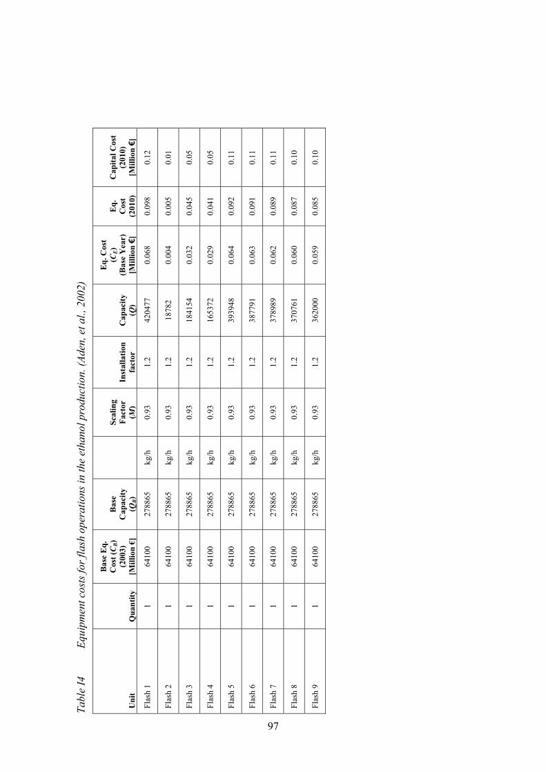
Tab

le I

4

Equ

ipm

ent c

osts

for

flas

h op

erat

ions

in th

e et

hano

l pro

duct

ion.

(A

den,

et a

l., 2

002)

Un

it

Qu

anti

ty

Bas

e E

q.

Cos

t (C

B)

(200

3)

[Mil

lion

€]

Bas

e C

apac

ity

(QB)

Sca

lin

g F

acto

r (M

) In

stal

lati

on

fact

or

Cap

acit

y (Q

)

Eq

. Cos

t (C

E)

(Bas

e Y

ear)

[M

illio

n €

]

Eq

. C

ost

(201

0)

Cap

ital

Cos

t (2

010)

[M

illio

n €

]

Fla

sh 1

1

6410

0 27

8865

kg

/h

0.93

1.

2 42

0477

0.

068

0.09

8 0.

12

Fla

sh 2

1

6410

0 27

8865

kg

/h

0.93

1.

2 18

782

0.00

4 0.

005

0.01

Fla

sh 3

1

6410

0 27

8865

kg

/h

0.93

1.

2 18

4154

0.

032

0.04

5 0.

05

Fla

sh 4

1

6410

0 27

8865

kg

/h

0.93

1.

2 16

5372

0.

029

0.04

1 0.

05

Fla

sh 5

1

6410

0 27

8865

kg

/h

0.93

1.

2 39

3948

0.

064

0.09

2 0.

11

Fla

sh 6

1

6410

0 27

8865

kg

/h

0.93

1.

2 38

7791

0.

063

0.09

1 0.

11

Fla

sh 7

1

6410

0 27

8865

kg

/h

0.93

1.

2 37

8989

0.

062

0.08

9 0.

11

Fla

sh 8

1

6410

0 27

8865

kg

/h

0.93

1.

2 37

0761

0.

060

0.08

7 0.

10

Fla

sh 9

1

6410

0 27

8865

kg

/h

0.93

1.

2 36

2000

0.

059

0.08

5 0.

10

97

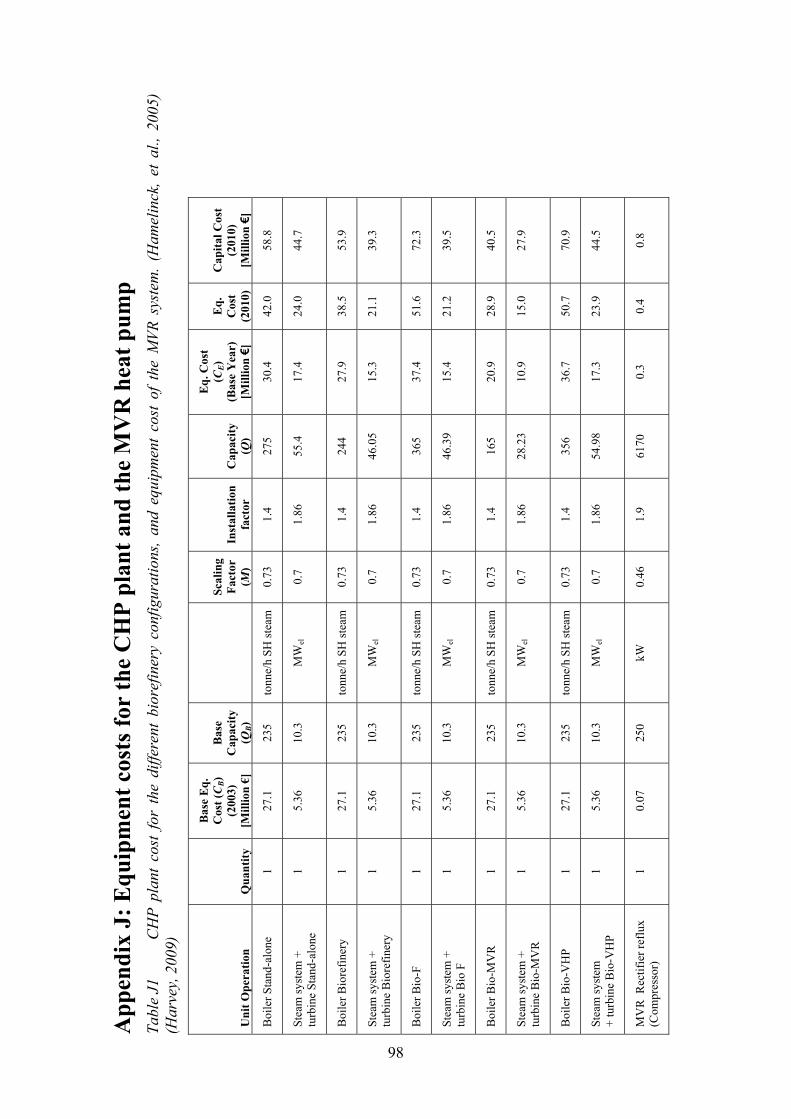
Ap

pen

dix

J:

Eq

uip

men

t co

sts

for

the

CH

P p

lan

t an

d t

he

MV

R h

eat

pu

mp

T

able

J1

C

HP

pla

nt c

ost

for

the

diff

eren

t bi

oref

iner

y co

nfig

urat

ions

, an

d eq

uipm

ent

cost

of

the

MV

R s

yste

m.

(Ham

elin

ck,

et a

l., 2

005)

(H

arve

y, 2

009)

Un

it O

per

atio

n Q

uan

tity

Bas

e E

q.

Cos

t (C

B)

(200

3)

[Mil

lion

€]

Bas

e C

apac

ity

(QB)

Sca

lin

g F

acto

r(M

) In

stal

lati

on

fact

or

Cap

acit

y(Q

)

Eq

. Cos

t (C

E)

(Bas

e Y

ear)

[M

illio

n €

]

Eq

. C

ost

(201

0)

Cap

ital

Cos

t (2

010)

[M

illio

n €

]

Boi

ler

Sta

nd-a

lone

1

27.1

23

5 to

nne/

h S

H s

team

0.

73

1.4

275

30.4

42

.0

58.8

Stea

m s

yste

m +

tu

rbin

e S

tand

-alo

ne

1 5.

36

10.3

M

Wel

0.7

1.86

55

.4

17.4

24

.0

44.7

Boi

ler

Bio

refi

nery

1

27.1

23

5 to

nne/

h S

H s

team

0.

73

1.4

244

27.9

38

.5

53.9

Stea

m s

yste

m +

tu

rbin

e B

iore

fine

ry

1 5.

36

10.3

M

Wel

0.7

1.86

46

.05

15.3

21

.1

39.3

Boi

ler

Bio

-F

1 27

.1

235

tonn

e/h

SH

ste

am

0.73

1.

4 36

5 37

.4

51.6

72

.3

Stea

m s

yste

m +

tu

rbin

e B

io F

1

5.36

10

.3

MW

el

0.7

1.86

46

.39

15.4

21

.2

39.5

Boi

ler

Bio

-MV

R

1 27

.1

235

tonn

e/h

SH

ste

am

0.73

1.

4 16

5 20

.9

28.9

40

.5

Stea

m s

yste

m +

tu

rbin

e B

io-M

VR

1

5.36

10

.3

MW

el

0.7

1.86

28

.23

10.9

15

.0

27.9

Boi

ler

Bio

-VH

P

1 27

.1

235

tonn

e/h

SH

ste

am

0.73

1.

4 35

6 36

.7

50.7

70

.9

Stea

m s

yste

m

+ tu

rbin

e B

io-V

HP

1

5.36

10

.3

MW

el

0.7

1.86

54

.98

17.3

23

.9

44.5

MV

R R

ecti

fier

ref

lux

(Com

pres

sor)

1

0.07

25

0 kW

0.

46

1.9

6170

0.

3 0.

4 0.

8

98

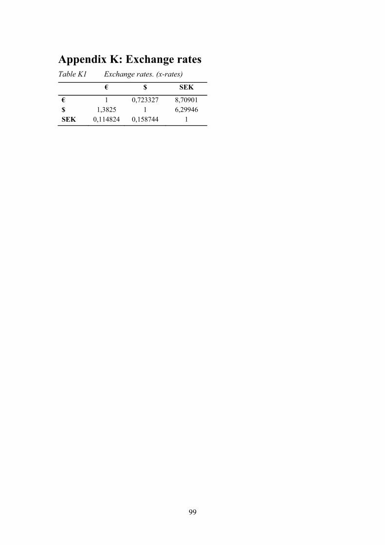
96

Appendix K: Exchange rates Table K1 Exchange rates. (x-rates) € $ SEK

€ 1 0,723327 8,70901 $ 1,3825 1 6,29946 SEK 0,114824 0,158744 1

99

Process integration study of a biorefinery producing...

Documents

Transcript of Process integration study of a biorefinery producing...