Proceedings of the Pelagic Longline Catch Rate Standardization Meeting
71
PROCEEDINGS OF THE PELAGIC LONGLINE CATCH RATE STANDARDIZATION MEETING February 12−16, 2007 Imin Conference Center University of Hawaii, Honolulu Simon D. Hoyle 1 , Keith A. Bigelow 2 , Adam D. Langley 1 , and Mark N. Maunder 3 . 1 Secretariat of the Pacific Community, Noumea, New Caledonia 2 Pacific Islands Fisheries Science Center, Honolulu, HI, USA 3 Inter-American Tropical Tuna Commission, La Jolla, CA, USA
Transcript of Proceedings of the Pelagic Longline Catch Rate Standardization Meeting

PROCEEDINGS OF THE PELAGIC LONGLINE CATCH RATE STANDARDIZATION MEETING
February 12−16, 2007
Imin Conference Center University of Hawaii, Honolulu
Simon D. Hoyle1, Keith A. Bigelow2, Adam D. Langley1, and Mark N. Maunder3.
1 Secretariat of the Pacific Community, Noumea, New Caledonia 2 Pacific Islands Fisheries Science Center, Honolulu, HI, USA 3 Inter-American Tropical Tuna Commission, La Jolla, CA, USA


Pelagic longline catch rate standardization meeting, Feb 2007
Table of Contents Introduction......................................................................................................................... 1
Summary of recommendations ........................................................................................... 2 Recommendations for stock assessments – 2007........................................................ 2 Recommendations for stock assessments – Longer term............................................ 3 Recommendations relating to PFRP project ............................................................... 5
Summary of meeting........................................................................................................... 6
1. Overview of longline effort standardizations in current Pacific HMS assessments ... 6
2. Models for standardizing longline effort: GLMs, GAMs, neural networks, and covariates .................................................................................................................. 10 Oceanographic variables ........................................................................................... 11 Model selection and model averaging....................................................................... 13 The dependent variable ............................................................................................. 14 Modelling variance.................................................................................................... 14 Missing values for covariates.................................................................................... 15
3. Models for standardizing longline effort: depth-related and habitat-related vulnerability .............................................................................................................. 16
4. Targeting ................................................................................................................... 19
5. Longline gear depth, shoaling and HMS vulnerability ............................................. 22
6. Longline CPUE simulations ..................................................................................... 24
7. Time-series changes in catchability: Quantifying technological improvements ...... 25
8. Regional weighting ................................................................................................... 26
9. Spatial considerations ............................................................................................... 26
10. Data: resolution, stratification, and data from other fleets (Korea, Taiwan, domestic)................................................................................................................... 29
References......................................................................................................................... 31
Appendix I: Agenda.......................................................................................................... 35
Appendix II: List of working and background papers ...................................................... 38
Appendix III: Abstracts..................................................................................................... 40
1. Overview of longline effort standardizations in current Pacific HMS assessments . 40 i. Application of catch and effort data in WCPO assessments - Adam
Langley ................................................................................................... 40 ii. Methods used to standardize longline catch and effort data in the EPO –
Mark N. Maunder and Simon D. Hoyle.................................................. 41 iii. Standardized CPUE of striped marlin caught by Japanese distant water
longliners in the North Pacific – Momoko Ichinokawa and Kotaro Yokawa ................................................................................................... 42
i

Pelagic longline catch rate standardization meeting, Feb 2007
2. Models for standardizing longline effort: GLMs, GAMs, neural networks and covariates .................................................................................................................. 42
iv. Incorporation of oceanographic data in the standardization of longline CPUE for the WCPO stock assessments – A. Langley .......................... 42
v. Aspects of model selection for GLMs applied to striped marlin in the Hawaii-based longline fishery (WP1) Jon Brodziak .............................. 43
vi. Analyses of Observed Longline Catches of Blue Marlin, Makaira nigricans, using GAMs with Operational and Environmental Predictors – K. Bigelow.............................................................................................. 43
vii. Dealing with missing values for covariates – Mark N. Maunder ........... 44
3. Models for standardizing longline effort: habitat-related and depth-related vulnerability .............................................................................................................. 44
viii. A method for inferring the depth distribution of catchability for pelagic fishes and correcting for variations in the depth of longline fishing gear – Peter Ward .............................................................................................. 44
ix. Developing indices of abundance using habitat data in a statistical framework – Mark N. Maunder, Michael G. Hinton, Keith A. Bigelow, and Adam D. Langley............................................................................. 45
x. Using statHBS with a multiple species approach – Minoru Kanaiwa... 46 xi. Does habitat or depth influence catch rates of pelagic species? – K.
Bigelow/M. Maunder.............................................................................. 47
4. Targeting ................................................................................................................... 47 xii. Hooks between floats and Japanese longline data; and joint analysis of
YFT and BET CPUE from Japanese longline data – S. Hoyle/A. Langley................................................................................................................ 47
5. Longline gear depth, shoaling and HMS vulnerability ............................................. 48 xiii. Pelagic longline gear depth and shoaling – K. Bigelow......................... 48 xiv. Pelagic longline fishing depth: Confronting catenary theory data with
depth observations from monitored longline fishing experiments (WP5) – Pascal Bach and Daniel Gaertner............................................................ 48
xv. Recent topics of tuna longline CPUE analysis within the National Research Institute of Far Seas Fisheries – Kotaro Yokawa.................... 49
xvi. Estimation of hook depth during near surface pelagic longline fishing using catenary geometry: theory versus practice (WP2) – Patrick Rice, Phil Goodyear, Eric D. Prince, Derke Snodgrass, and Joe Serafy.......... 49
xvii. Aspects of the Physical Habitat of Atlantic Blue Marlin: Predicting Vulnerability to Longline Fishing Gear (WP3) – Phil Goodyear, Jiangang Luo, Eric D. Prince, Derke Snodgrass, Eric Orbesen, and Joe Serafy. ..................................................................................................... 50
xviii. The COPAL software: a tool to estimate both hook depths and the maximum fishing depth of longlines according to setting tactic information – P. Bach/D. Gaertner ......................................................... 50
6. Longline CPUE simulations ..................................................................................... 51 xix. Simulation and analysis of longline catch and effort data – P. Goodyear
................................................................................................................ 51
ii

Pelagic longline catch rate standardization meeting, Feb 2007
7. Time-series changes in catchability: Quantifying technological improvements ...... 52 xx. An overview of historical changes in the fishing gear and practices of
pelagic longliners (WP4) – P. Ward and S. Hindmarsh. ........................ 52
8. Regional weighting ................................................................................................... 53 xxi. Regional weighting – S. Hoyle ............................................................... 53
9. Spatial considerations ............................................................................................... 53 xxii. Consideration of a range of spatial effects that may influence CPUE
indices for yellowfin and bigeye in the WCPO – A. Langley ................ 53 xxiii. Filling in missing cells by integrating CPUE standardization with a
population dynamics model – M. Maunder ............................................ 54 xxiv. Relative abundance trends of tuna and billfishes in the Pacific Ocean
inferred from Japanese longline spatial catch and effort data (WP6) – Robert Ahrens ......................................................................................... 55
Appendix IV − Summary of gear configuration from observer programs and research cruises ............................................................................................................................... 56
Appendix V − Summary of longline standardization methods and analyses ................... 58
Appendix VI − List of participants ................................................................................... 65
iii
Pelagic longline catch rate standardization meeting, Feb 2007
Introduction The Pelagic Longline Catch Rate Standardization meeting was held at the Imin Conference Center, University of Hawaii, Honolulu, from February 12−16 2007. The meeting was jointly hosted by the Secretariat of the Pacific Community (SPC) and Pelagic Fisheries Research Program (PFRP) funded project "Performance of Longline Catchability Models in Assessments of Pacific Highly Migratory Species". Workshop convenors were Keith Bigelow of the US National Marine Fisheries Service, and Simon Hoyle of the Oceanic Fisheries Programme, SPC. Funding and support were also provided by the Western and Central Pacific Fisheries Commission, the Pacific Islands Oceanic Fisheries Management Project (itself funded by the Global Environment Facility), and the US National Marine Fisheries Service.
The objectives of the meeting were to provide a technical review of current (and alternative) longline CPUE standardization techniques used for the yellowfin and bigeye stock assessments in the Western and Central Pacific Ocean (WCPO), and to formulate a research plan to meet the objectives of the PFRP longline catchability project. SPC had an additional objective of obtaining some guidance on the analysis of CPUE data from the longline fleet, and addressing the key issues identified by WCPFC Scientific Committee 2. The standardized longline data are one of the most influential components in the stock assessments for yellowfin and bigeye tuna in the WCPO.
John Sibert of the University of Hawaii welcomed participants. The meeting was chaired by Keith Bigelow. Adam Langley of SPC chaired discussions of issues directly related to SPC stock assessments on days 4 and 5. Simon Hoyle was rapporteur, and notes were also provided by Mark Maunder, Adam Langley, and Keith Bigelow.
The meeting was attended by 24 scientists from a number of organizations: the SPC (Don Bromhead, Simon Hoyle, Adam Langley, Brett Molony), Inter-American Tropical Tuna Commission (Mark Maunder), Institut de Recherche pour le Développement (Pascal Bach, Daniel Gaertner), CSIRO (Rob Campbell), Bureau of Rural Sciences (Australia) (Peter Ward, Emma Lawrence), Western and Central Pacific Fisheries Commission (SungKwon Soh), Japanese Far Seas Fisheries Lab (Kotaro Yokawa, Momoko Ichinokawa), Tokyo University of Agriculture (Minoru Kanaiwa), and the US National Marine Fisheries Service (Keith Bigelow, Jon Brodziak, Emmanis Dorval, Marco Kienzle, Pierre Kleiber, Kevin Piner). In addition, Phil Goodyear (US) and three fisheries staff from Pacific Island countries and territories attended the meeting (Jone Amoe, Pam Maru, and Cedric Ponsonnet).
1

Pelagic longline catch rate standardization meeting, Feb 2007
Summary of recommendations
Recommendations for stock assessments – 2007
Regional weighting factors - Consider a time period from 1975 to 1986. Re-weight using 1960-1974 and 1975-
1986, and compare outcomes. Outcomes may differ between species; e.g. 1960-74 may be better for yellowfin
- Consider including interaction terms in the model, including region and hooks between floats (HBF)
Data resolution, and analyses using other datasets
- Set by set analyses for target species are recommended, both to compare indices with those from aggregated data and to investigate factors that might affect catch rates. Suitable data sources include:
o Hawaii-based longline data: e.g. moon phase, time of day of set, bait type, vessel id, vessel length. Compare with coarser 1º and 5º monthly data..
o Within-EEZ logsheet data for all longline fleets, particularly regarding gear configuration
- Spatial and effort contraction of the Japanese longline fishery over the past decade makes it important to include other datasets in order to develop CPUE indices relevant for the entire WCPO.
- Compare nominal indices of the Japanese fleet and other fleets at appropriate spatial and temporal scales.
- Explore standardization for Korea and Taiwan CPUE for a global CPUE index - Where possible, indices for all countries to be made available.
Examine sensitivities of the stock assessment models to assumptions in the GLM.
- Examine sensitivity to the assumption that HBF=5 before 1975. - Examine sensitivity to the assumption that HBF effects are equivalent throughout
the time period, given that longline material specific gravity may have changed for many vessels during and after 1993.
- Examine sensitivity to plausible increases in fishing power. Define ‘plausible’, perhaps via a paper from Peter Ward. See also paper by Miki Ogura on pole and line fishery, presented to SCTB several years ago.
- Attempt to standardise using data only from main gear configurations – this implies subdividing the CPUE index. Is data for specific gear configurations available? Yokawa-san will ask Okamoto-san, and provide if it is reliable.
Reporting at the WCPFC Scientific Committee
- Report against biological hypotheses – compare model parameterization to biologically-based expectations, such as HBF.
- Explain implications of statistical assumptions in terms of biology, fleet dynamics, and population dynamics.
2
Pelagic longline catch rate standardization meeting, Feb 2007
- Compare depth distribution from archival tags with depth/habitat at capture on longlines for all species.
Recommendations for stock assessments – Longer term
Spatial effects - Develop standardization using spatial backfilling – investigate effects of
alternative approaches, (e.g. Campbell et al, Ahrens PhD research, and Maunder - combining pop dynamics and GLM).
- Develop methods to include uncertainty in spatial back-filling approaches. - Model population dynamics of region 3 at a smaller spatial resolution, to examine
potential effects of spatial heterogeneity in fishing effort and population structure. - Compare results of a simple GLM, an area-weighted model, and an abundance-
weighted model. - Given the geographical diversity of region 3, and the limited information
regarding the western part of region 3, carry out a sensitivity analysis to removing the western part from the CPUE analysis.
Modelling approaches
- Determine which of the currently available methods for standardizing CPUE are generally applicable and the conditions under which they will perform better than other methods.
- When using simulation analysis, start with simple models to test the utility of existing methods and test where the methods break down. Build in increasing complexity to determine their performance in realistic applications.
- Review literature on CPUE standardization, and note covariates and factors for which standardization substantially changes the year effect from nominal CPUE.
- Combine GLM with pop dynamics model – examine outcomes via simulation
Missing covariates, - Take a statistical approach to estimating missing observations, using the EM
algorithm for example.
Time horizon - Given the uncertainty about the factors affecting pre-1975 CPUE, consider
starting assessments in 1975 instead of 1952, or at least using only the post-1975 period to infer long-term average recruitment. Consider the implications for the assessment model and for management.
Targeting
- Cluster analysis for Japanese data to compare the observed clustering with HBF and area targeting information, in order to see how well the clustering approach works. This can be used to validate the approach for other fleets.
3

Pelagic longline catch rate standardization meeting, Feb 2007
- Market demand (by species, fish condition, fat content (also affected by area & time of year)) can affect targeting. Consider how market demand can be integrated into the determination of targeting
- Consider how oceanography can be integrated into the determination of targeting. - Review approaches for including data from other species in GLMs. - Investigate simultaneous standardization across species to resolve changes in
targeting behaviour. - Investigate analyses of targeting that include data from multiple fleets.
Data resolution, and analyses using other datasets - Develop CPUE indices for all countries/fleets where longline data exist.
Data requirements
- Determine the status of current data holdings, including identifying the nature and magnitude of deficiencies, and determine the priority for data collection for current model applications.
- Identify what data should be collected in the logbooks for all fleets to improve our ability to capture changes in the relationship between catch and effort, and to ensure the ability to maintain the information context and usefulness of long-term data series.
Quantify changes in gear configuration, and time series changes in catchability
- Further development to include additional species and to estimate actual gear depth using multi-species statHBS approach.
- Develop alternative likelihoods for multi-species approach. - Investigate possibility that major discontinuities (10−25%) in CPUE indices are
related to introduction of new technologies. - Examine CPUE indices to investigate the possibility of simultaneous changes in
catch rates across multiple oceans / species. - Investigate the effectiveness of a variety of equipment, such as acoustic Doppler
current profiler (ADCP). - Review Japanese research reports for information on gear configuration changes
in 1975, 1993, and at other times. - Investigate possible changes in gear selectivity at 5 HBF pre- and post-1975 for
Japanese longline vessels in the Pacific (as noted for similar vessels in the Indian and Atlantic Oceans).
Sensitivity analyses to known or potential changes in gear configuration
- Mainline composition changed with the introduction of monofilament in 1990s. HBF changed, but depth may not have. This change was associated with diversification of gear configurations. Examine potential sensitivity of year effect to this change.
- Estimate separate catchabilities before and after 1975 in the assessment model, sharing selectivity.
4

Pelagic longline catch rate standardization meeting, Feb 2007
Recommendations relating to PFRP project
Data suggestions for observer programs - Incorporate details from table 1 in background paper 10. - Validate longline gear depth with temperature depth recorders (TDR’s). - Collect gear attributes such as line types, hook types and sizes, weights, weighted
swivels, bait type etc. - Use more hook timers to validate time of capture. - Observers to report which hook each fish was caught on, and time of day caught. - Geographical coordinates at start and end of haul. - Validate logbooks using observer data.
Other data collection recommendations
- National scientists to describe fishery gear configurations, particularly upon introduction of new gear technologies.
- Possible provision of Japanese longline data stratified by material type. Oceanographic effects
- GLM with CPUE as a function of oceanography alone, without temporal and spatial effects, to explore how oceanography (which is confounded with space and time) may affect catch or CPUE.
- Review availability of fine-scale spatial and temporal oceanographic data, especially remotely sensed rather than model-derived data. Compare coherence of both data types, and investigate biases.
- Use existing and develop new algorithms, at appropriate spatio-temporal resolution, to describe the evolution, decay, and persistence of features such as eddies and frontal structures, for both fish accumulation and fishery targeting.
Model selection
- Investigate alternative hypotheses, and use model averaging to integrate over model selection uncertainty where it occurs.
- Develop tests appropriate for determining which standardization methods provide the best index of relative abundance from a set of candidate methods.
- Evaluate the performance of candidate tests using simulation analysis. Gear dynamics
- Further experiments to quantify longline shoaling due to horizontal current shear and changes in sag ratio.
- Characterize intra-set variability in gear depth, and statistically determine optimum number of TDR’s given variability.
- Investigate functional relationship relating depth fished with HBF/longline material.
5

Pelagic longline catch rate standardization meeting, Feb 2007
Summary of meeting
1. Overview of longline effort standardizations in current Pacific HMS assessments
A number of different methods have been used for standardizing CPUE data for highly migratory species in the Pacific. Methods currently used for WCPFC stock assessments of the Western and Central Pacific Ocean (WCPO) were summarized by Adam Langley (see abstract page 40). For further detail see Langley et al. (2005).
Japanese longline data are critical for developing these indices of abundance, because of their large-scale spatial coverage, the length of the available time series, and the consistency of reporting, which are not matched by any other time series of catch and effort data. There are also long time series of purse seine catch and effort data, but due to the nature of the fishing method, purse seine data are less appropriate for developing indices of abundance. However, the contraction of the Japanese longline fishery in recent years, which continues, makes it increasingly important to evaluate the integration of data from other fisheries into standardizations.
The WCPO is generally modelled as six separate regions, and the CPUE standardization is carried out separately for each region, and reweighted later (see reweighting, section 8). The six regions can be viewed as six separate assessments, but parameters are shared among the regions, and inter-region movement rates estimated.
Catch and effort are aggregated spatially and temporally by 5x5º - month, and number of hooks between floats (HBF). Catch by stratum is modelled as a function of effort and other parameters. The relationship between catch and effort is modelled as a third order polynomial, to accommodate possible saturation at high effort and searching behaviour in strata with low effort; although these effects will be somewhat complicated by the inclusion of HBF in the stratification. The relationship is estimated to be linear over most of the range of the data, and abundance indices are similar when the relationship is constrained to be linear.
For yellowfin in the WCPO, the GLM models generally find the expected relationship between CPUE and HBF, i.e. CPUE generally declines with increasing HBF (increased hook depth). However, the bigeye CPUE index does not reveal the converse trend that would be expected from our understanding of the depth distribution of the species and changes in target practice. There is concern that the temporal trend in increased HBF (and therefore increasing bigeye catchability) is not captured by the GLM models, and that the resulting CPUE indices may be positively biased. Catch rates may be influenced by factors that interact with HBF, but are not included in the aggregated data. Analyses of set-by-set data are suggested, as they may provide relevant insights.
Methods used in the Eastern Pacific Ocean (EPO) over the past decade were described by Mark Maunder (see abstract page 41). The most recent methods are described by Hoyle and Maunder (2006). The IATTC has applied multiple methods to standardize catch rates for yellowfin and bigeye tuna in the EPO, most recently using a delta lognormal GLM approach (Hoyle and Maunder 2006). The most important conclusion to be drawn from the results is that almost all of the methods used, including nominal CPUE, produce
6

Pelagic longline catch rate standardization meeting, Feb 2007
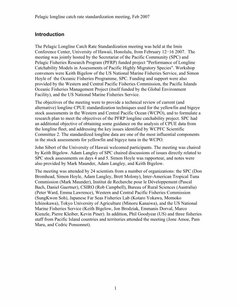
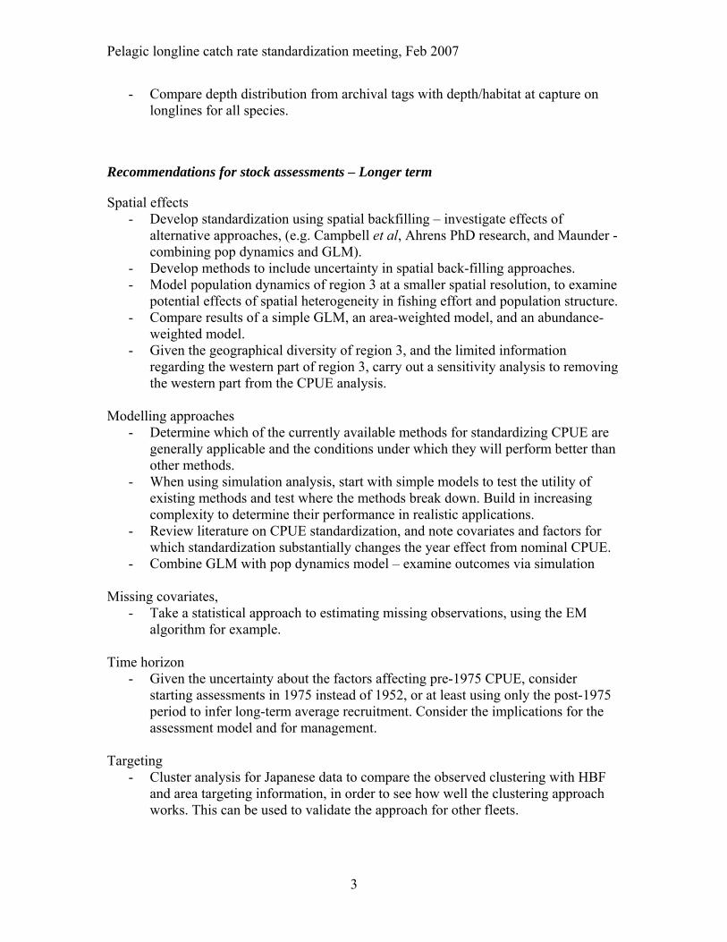
similar results for the parameter of interest: the quarterly abundance index. Only the deterministic habitat based standardization model (Hinton and Nakano 1996) has produced a substantially different abundance index (Maunder et al. 2002). The explanatory variables included in the EPO model have generally not affected the relative index of abundance (Figure 1−2). In the WCPO, however, the yellowfin index of abundance has been modified by the explanatory variables HBF, bigeye CPUE, and 5º square (Figure 3), resulting in changes to management quantities.
YFT
0
0.5
1
1.5
2
2.5
3
3.5
1970 1975 1980 1985 1990 1995 2000 2005Year
Sta
ndar
dise
d C
PU
E
2000/1 2002 2003 2004/5 2006
Figure 1: Indices of yellowfin tuna abundance in the EPO resulting from standardization of CPUE data from 2000 to 2006, using the following methods: 2000−2001 nominal CPUE; 2002 deterministic HBS; 2003−2004 neural networks; 2005 delta gamma GLM; 2006 delta lognormal GLM.
7

Pelagic longline catch rate standardization meeting, Feb 2007
BET
0
0.5
1
1.5
2
2.5
1970 1975 1980 1985 1990 1995 2000 2005Year
Sta
ndar
dise
d C
PU
E
2000 2001 2002 2003 2004 2005 2006
Figure 2: Indices of bigeye tuna abundance in the EPO resulting from standardization of CPUE data from 2000 to 2006, using the following methods: 2000−2001 regression trees; 2002 deterministic HBS; 2003−2004 neural networks; 2005 statistical HBS; 2006 delta lognormal GLM.
1950 1960 1970 1980 1990 2000
0.0
0.5
1.0
1.5
2.0
CP
UE
inde
x
Nom ina lGLM , HB F + be t_propGLM , HB FGLM , HB F + be t_cpue
YF T R e g io n3
Figure 3: Comparisons among standardizations of yellowfin CPUE in region 3 of the WCPO. Standardizing by HBF gives an index of abundance quite different from nominal CPUE. Adding ‘proportion bigeye in the catch’ further modifies the trend, while adding ‘bigeye CPUE’ has less effect.
8
Pelagic longline catch rate standardization meeting, Feb 2007
Momoko Ichinokawa’s presentation (see abstract page 42), on standardization of CPUE data for striped marlin in the North Pacific, a non-target but retained species, revealed some difficulties. Rapid decline of nominal CPUE around the Hawaiian islands in the Central Pacific during the early 1970’s was inconsistent with CPUE trends elsewhere. The decline may have been affected by gear configuration changes. Japanese longliners had not been operating in the Central and Eastern Pacific since the 1960’s, and gear configurations changed dramatically between the 1960’s and 1970’s. However, introducing set by set data (with gear configuration information) for 1962−1966 and 1975−2005 into the standardization did not explain the rapid decline. Further study is needed of historical changes of gear configuration in Japanese longline fisheries and their possible effects on catch rates. Catch rates by species can also vary markedly due to the targeting practices of individual vessels, and this deserves further exploration.
A further problem was related to an area of the eastern Pacific, thought to be a spawning area, with striped marlin catch rates about 10 times those elsewhere. Longline effort in this area has been decreasing since the 1970’s, with little effort since 1990; a change partly caused by a shift of target species in the Eastern Pacific from striped marlin to bigeye tuna. Such situations sometimes occur with bycatch species.
This change raised several issues. First, the CPUE trend in this area of high abundance may not be the same as the trend elsewhere. If this is the case, then the area of high abundance can be standardized separately; or a single standardization can include an interaction term between time and location, and the locations reweighted later. Reweighting in such cases should be by abundance rather than by area. This issue is dealt with in more detail in section 9 on spatial considerations. However, for some species, catch rates in spawning areas tend to be hyperstable due to aggregation of fish from other areas at certain times of year. This type of hyperstability can be dealt with by ignoring the CPUE during the spawning season, and only using the CPUE when the fish are dispersed. Alternatively, the supposed spawning area can be modelled separately and the effect of hyperstability modelled explicitly.
Second, the lack of effort in this high abundance area leaves overall abundance very uncertain – see the spatial considerations section 9 for more discussion of this issue. The uncertainty caused by the shift of target species and the biased distribution of fishing efforts should be quantitatively evaluated, with a view to making changes for future stock assessments. Despite the gradual shift in targeting from marlin to tunas, an expected negative correlation between CPUE of these species was not apparent.
The above highlights the need to develop methods to model the effects of, and indicators of, targeting, so that targeting can be taken into consideration in the CPUE standardisation.
See also Molony (2005) for information on factors affecting billfish catches by longline fisheries in the WCPO.
9

Pelagic longline catch rate standardization meeting, Feb 2007
2. Models for standardizing longline effort: GLMs, GAMs, neural networks, and covariates
Many explanatory variables can be used to standardize CPUE data. These variables can come from the process that was used to record the CPUE data (e.g. from logbooks) or from other sources which can be mapped to the CPUE data (e.g. environmental data from remote sensing; general circulation models). The type of variables available will often depend on the spatial and temporal resolution of the data set that is used.
It is not clear which explanatory variables should be given the highest priority for reporting in data and use in analyses. It might be useful to review all available CPUE standardization analyses to identify which explanatory variables have been found to be influential, and use those as a recommended set of variables to consider. However, factors not yet considered may in future be found to be influential.
If a large number of variables are considered for inclusion in the model, many of these might be correlated. Methods to eliminate correlated variables may be useful. However, if the objective of the analysis is to produce an index of abundance and not to identify important factors, having correlated covariates may not be so important.
Care should be taken to ensure that covariates are only included if they influence catchability, rather than abundance. For example, if it was found that an oceanographic parameter explained significant variation in yellowfin catch rates via its effect on abundance, and this parameter exhibited a long term trend, then the relationship would have important ecological ramifications. However, it should not be included in the standardization to produce an index of abundance, because including the parameter would remove some of the abundance trend. Additional investigations, possibly in conjunction with ocean modelers, should be undertaken to determine if the change in CPUE is due to changes in abundance, or due to changes in catchability associated with an oceanographic variable with a long term trend.
Key covariates in the model with a strong temporal trend, such as the HBF variable which steadily increases over time, may be confounded with the year effect. Without sufficient within-year overlap in the HBF categories, the model may not be able to separate the trend in catchability from the trend in abundance. Overlap between the different levels of the covariate in some years will avoid confounding with the year effect. The same argument applies to oceanographic variables – although this is probably not a serious problem when fishing occurs over broad habitat areas.
The form of the covariate used in the model also needs to be considered. GAMs are good for visualizing the relationship with covariates. The forms suggested by the GAM can then be used for formulating the GLM model. If a GAM is used to generate the index of abundance, a categorical variable should be used for the year effect, because the stock assessment model smoothes the year effect and it should not be smoothed by the GAM beforehand.
CPUE data often contain many zero catch records, particularly for minor species and data at fine spatio-temporal scales. GLMs with a lognormal error distribution cannot accept zeros; there are several ways of dealing with this. When there are few zeroes they can be omitted (e.g. Langley et al. 2005) and the results checked to see if there is any effect.
10

Pelagic longline catch rate standardization meeting, Feb 2007
Checking can be done by comparing results with other approaches, such as a delta-based or zero-inflated analysis. Delta approaches (such as the delta lognormal, e.g. Hoyle and Maunder 2006) model the zeros explicitly with a mixture model that includes a binomial component – taking care to model the probability of catching nothing as a function of effort. Zero-inflated approaches (e.g. the zero-inflated negative binomial, Minami et al. 2007) also use a mixture approach. Given the same distribution for non-zeroes, delta or zero-inflated approaches are statistically more appropriate than omitting zeroes, but the advantages of omitting the zeroes include simpler, more flexible, faster and less memory-hungry analyses, and easier access to variance estimates.
Count-based distributions such as the Poisson and negative binomial can also cope with zero values. Lack of independence and consequent over-dispersion in catch rate data usually make the more flexible negative binomial distribution more appropriate than the Poisson. However, many processes can contribute to observed zero catches, and there are often more zeroes than will fit even the negative binomial distribution. Momoko Ichinokawa’s preliminary modelling of set by set data for striped marlin found that the negative binomial distribution was inadequate and resulted in a skewed distribution of model residuals. The zero-inflated negative binomial can be recommended as a good approach for modelling bycatch and minor species data (e.g. Minami et al. 2007), which are often characterized by many zeroes and some quite large catches.
Oceanographic variables
Oceanographic variables are potentially important in the GLM models for yellowfin, bigeye and South Pacific albacore. A PFRP-funded workshop was held in Honolulu in May 2002 to consider the use of oceanographic data in longline standardizations (Kleiber 2002). However, the relationship between oceanographic variables and catch rates is circumscribed by the resolution of the available oceanographic and fishery data. Catch and effort data included in the WCPFC assessments are limited by the resolution of the early data to a relatively broad spatial (5º) and temporal (monthly) scale. Oceanographic data, derived from physical-biogeochemical models, are available at a comparable resolution. Averages over broad spatial and temporal scales do not represent the fine-scale heterogeneity that may exist (and affect catch rates) in the environment, fish distribution, and vessel distribution. Similar arguments are made to explain the poor performance of the deterministic habitat-based standardization (HBS) models.
Analysis of Japanese longline data of bigeye and yellowfin catch at a 1º - month scale, presented by Adam Langley (see abstract page 42), found statistically significant and biologically meaningful relationships between catch rates and a range of oceanographic variables. However, including these variables in the GLM model did not alter the index of abundance. Albacore catch rates showed some relationship with current speed and direction, but not to the extent that the index of abundance was affected.
Even with fine-scale fishery data, analyses are limited by the resolution of the oceanographic data. Marco Kienzle reported that, in modelling set by set data for albacore in Samoan waters, oceanographic variables explained only 1% of the variation. The 1º - month stratum represents an average of the oceanography, and fish movement and targeting occurs at much smaller temporal and spatial scales. Research to look at
11

Pelagic longline catch rate standardization meeting, Feb 2007
oceanographic effects on catch rate on smaller temporal and spatial scales is needed. Such research is currently under way at the CSIRO, Australia, using fine-scale remotely sensed data averaged over two days and 2-3 km.
The most accurate oceanographic data are sourced from remote sensing. Oceanographic data are all processed to some degree and contain error and uncertainty, but the level of uncertainty in available oceanographic products is usually not included in CPUE analyses.
Consistent oceanographic variation between locations is confounded with spatial and seasonal effects (depending on the spatial extent of the data) and broad scale oceanographic changes within regions are confounded with the abundance index. It may therefore be useful to investigate relationships between oceanography and catch rate at the 1º- month scale, but without fitting 5º-month square or year-quarter as explanatory variables.
Different data products are likely to be suitable for different species. Oceanographic influences on species, such as bigeye tuna, that interact with processes occurring at greater depth may be harder to find, because data precision and accuracy decline with depth. It may be easier to find oceanographic effects on catch for species that spend more time at the surface, such as yellowfin, skipjack, and billfish. A model derived from oceanographic data is likely to be much more precise if it uses data from the last two decades than using data from an earlier period.
Most oceanographic data are included into CPUE standardisation in simplistic forms (e.g. SST, current speed), but CPUE may be influenced by more complex oceanographic features (e.g. fronts). Research is needed to develop methods to quantify these features so that they can be included in CPUE standardisation. For example, Japanese longline fishers report that fish accumulate into an eddy over time, so the evolution, persistence and decay of the eddy should be considered as well as its current state.
Including oceanographic data in GLM models is not likely to account for increases in fishing efficiency associated with effort directed at fine-scale oceanographic features with higher tuna catch rates. Such increases in catchability of tuna are likely to have occurred through the adoption of remote sensing products (e.g. SST maps) available to the longline fleet. Any attempt to resolve these trends with oceanographic data would require both oceanographic and fisheries data at a much finer spatial and temporal scale than is currently available. A more useful approach may be to focus on the technology on the vessels. Keith Bigelow (see abstract page 43) presented a comparison of GAMs for set-by-set observer data on blue marlin catches, fitted entirely with operational or environmental variables. A model with operational variables explained 33% of the null deviance, while environmental variables explained 20%. Nevertheless, the inclusion of the oceanographic data in the current GLM models does provide the potential to increase our insights into the habitat preferences of these species.
Given the number of environmental variables available for comparison with catch rates, spurious correlations may be found by chance. Relationships should be investigated based on assumptions about the underlying processes. Since they derive from biologically determined species behaviour patterns, relationships between environmental variables and catch rates are likely to be consistent between oceans.
12

Pelagic longline catch rate standardization meeting, Feb 2007
Model selection and model averaging
Selecting covariates to include in a model is an important part of standardizing CPUE data. However, with the plethora of different methods to standardize CPUE data, methods are needed to determine which method is appropriate. Standard statistical methods, such as the Akaike Information Criterion (AIC), can be used to test between many of the methods as well as to choose which covariates to include. These methods can also be used for model averaging, which in some situations provides better results. The resulting increase in uncertainty is often more realistic, with greater predictive accuracy. Jon Brodziak (see abstract page 43) presented an application of model averaging to the standardization of CPUE data.
However, model selection is not always important because including more covariates than indicated by standard model selection criteria generally does not substantially influence the estimated index of abundance. Including irrelevant explanatory variables generally only influences the results if it explains some of the variation that should be attributed to abundance. The effect of including covariates on the standard errors of index of abundance is less important because the standard errors are usually inflated in the stock assessment models to account for unexplained variation in catchability and other model processes.
In subsequent discussions it was pointed out that if the different models produce very different results, and particularly if the differences have important implications for management, then it may be better to present both results rather than an average. In such cases it is possible to include model uncertainty in the processes used to produce management advice.
Further model validation and selection can be carried out using cross validation and a holistic approach (Hinton and Maunder, 2003 ). This holistic approach is used to check whether the index of abundance is consistent with the other data (e.g. length frequency) and the population dynamics represented by the stock assessment model.
It is important to keep in mind that the goal of standardization is usually to produce an index of abundance. Where different methods produce essentially the same index, features such as ease of use, and the clarity of the underlying assumptions, become important. For example, the delta lognormal GLM gives a very similar index of abundance for WCPO yellowfin tuna to the lognormal GLM with zero-catch observations deleted. However, the lognormal GLM runs much more quickly in R, estimates variances, uses less memory, and is a better research tool, since it is easier to examine and interpret explanatory variables. Similarly, neural networks have produced very similar indices of abundance to GLM approaches for yellowfin and bigeye tuna in the EPO, but the neural network approach does not facilitate interpretation of the explanatory variables.
Such practical considerations are reinforced by the point that fishery data are often modelled as statistically independent, when they are not. Data may be overdispersed relative to the assumed distribution (as indicated by the magnitude of the deviance relative to the degrees of freedom (Venables and Ripley 2002, p 208), because the aggregated 5º - month cells share features such as trips and vessels, and trip and vessel
13
Pelagic longline catch rate standardization meeting, Feb 2007
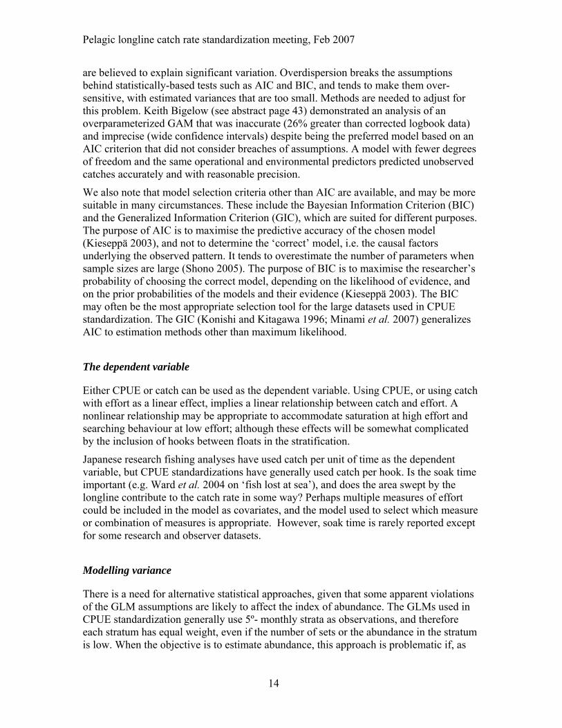
are believed to explain significant variation. Overdispersion breaks the assumptions behind statistically-based tests such as AIC and BIC, and tends to make them over-sensitive, with estimated variances that are too small. Methods are needed to adjust for this problem. Keith Bigelow (see abstract page 43) demonstrated an analysis of an overparameterized GAM that was inaccurate (26% greater than corrected logbook data) and imprecise (wide confidence intervals) despite being the preferred model based on an AIC criterion that did not consider breaches of assumptions. A model with fewer degrees of freedom and the same operational and environmental predictors predicted unobserved catches accurately and with reasonable precision.
We also note that model selection criteria other than AIC are available, and may be more suitable in many circumstances. These include the Bayesian Information Criterion (BIC) and the Generalized Information Criterion (GIC), which are suited for different purposes. The purpose of AIC is to maximise the predictive accuracy of the chosen model (Kieseppä 2003), and not to determine the ‘correct’ model, i.e. the causal factors underlying the observed pattern. It tends to overestimate the number of parameters when sample sizes are large (Shono 2005). The purpose of BIC is to maximise the researcher’s probability of choosing the correct model, depending on the likelihood of evidence, and on the prior probabilities of the models and their evidence (Kieseppä 2003). The BIC may often be the most appropriate selection tool for the large datasets used in CPUE standardization. The GIC (Konishi and Kitagawa 1996; Minami et al. 2007) generalizes AIC to estimation methods other than maximum likelihood.
The dependent variable
Either CPUE or catch can be used as the dependent variable. Using CPUE, or using catch with effort as a linear effect, implies a linear relationship between catch and effort. A nonlinear relationship may be appropriate to accommodate saturation at high effort and searching behaviour at low effort; although these effects will be somewhat complicated by the inclusion of hooks between floats in the stratification.
Japanese research fishing analyses have used catch per unit of time as the dependent variable, but CPUE standardizations have generally used catch per hook. Is the soak time important (e.g. Ward et al. 2004 on ‘fish lost at sea’), and does the area swept by the longline contribute to the catch rate in some way? Perhaps multiple measures of effort could be included in the model as covariates, and the model used to select which measure or combination of measures is appropriate. However, soak time is rarely reported except for some research and observer datasets.
Modelling variance
There is a need for alternative statistical approaches, given that some apparent violations of the GLM assumptions are likely to affect the index of abundance. The GLMs used in CPUE standardization generally use 5º- monthly strata as observations, and therefore each stratum has equal weight, even if the number of sets or the abundance in the stratum is low. When the objective is to estimate abundance, this approach is problematic if, as
14
Pelagic longline catch rate standardization meeting, Feb 2007
seems to be the case, the trends of high and low abundance strata are not parallel. The weight of each stratum should be related to its relative abundance, but uncertainty (a function of effective sample size and CPUE variability) in its estimates must also be considered. Some strata may have more CPUE variability than others due to the nature of those strata (e.g. more variable environments). Therefore, the likelihood should be weighted differently. One method to do this is to modify the variance of the likelihood function. The variance could be modelled as a function of the effort or covariates.
Missing values for covariates
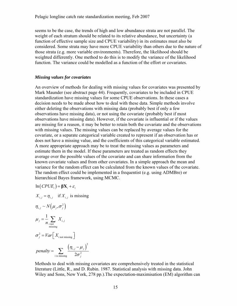
An overview of methods for dealing with missing values for covariates was presented by Mark Maunder (see abstract page 44). Frequently, covariates to be included in CPUE standardization have missing values for some CPUE observations. In these cases a decision needs to be made about how to deal with these data. Simple methods involve either deleting the observations with missing data (probably best if only a few observations have missing data), or not using the covariate (probably best if most observations have missing data). However, if the covariate is influential or if the values are missing for a reason, it may be better to retain both the covariate and the observations with missing values. The missing values can be replaced by average values for the covariate, or a separate categorical variable created to represent if an observation has or does not have a missing value, and the coefficients of this categorical variable estimated. A more appropriate approach may be to treat the missing values as parameters and estimate them in the model. If these parameters are treated as random effects they average over the possible values of the covariate and can share information from the known covariate values and from other covariates. In a simple approach the mean and variance for the random effect can be calculated from the known values of the covariate. The random effect could be implemented in a frequentist (e.g. using ADMBre) or hierarchical Bayes framework, using MCMC.
( )ln i iCPUE iε= +βX
, , ,if is missingi j i j i jX Xη=
( )2, ~ ,i j j jNη μ σ
,i not missing
1j i jX
nμ = ∑
2i not missingj Var Xσ ⎡ ⎤= ⎣ ⎦
( )2
,2
i is missing 2i j j
j
penaltyη μ
σ−
= ∑
Methods to deal with missing covariates are comprehensively treated in the statistical literature (Little, R., and D. Rubin. 1987. Statistical analysis with missing data. John Wiley and Sons, New York, 278 pp.).The expectation-maximisation (EM) algorithm can
15
Pelagic longline catch rate standardization meeting, Feb 2007
be used to implement the methods. When imputing the missing values, the relationship to other covariates needs to be considered. If the covariate is missing for a reason, then it may not be appropriate to delete the data points.
3. Models for standardizing longline effort: depth-related and habitat-related vulnerability
Catch rates and species caught by the longline fishing fleet can be influenced by the habitat in which they deploy their gear. A catch rate of a species will increase if the gear is deployed in the habitat in which that species prefers to feed. The fleet can use setting techniques to modify the vertical structure of the longline gear, such as by changing the number of hooks between floats. Environmental factors can change the vertical structure of the habitat, or the depth at which the gear fishes (e.g. through shoaling caused by currents). Standardization of longline CPUE data should consider the habitat that gear is fishing.
Habitat-based standardization was initially developed using a deterministic approach, with depth and temperature data from archival tags the primary sources of habitat information (Hinton and Nakano 1996, detHBS). A similar methodology was applied to depth information from detailed catch by hook position data (Ward and Myers 2005; see abstract page 44). A statistical approach for habitat-based standardization (statHBS) has also been developed (Maunder et al. 2006; see abstract page 45).
Deterministic habitat-based standardization matches the depth of the gear (from the catenary curve) with environmental data (from general circulation models) and the habitat preference of the species of interest to estimate effective longline effort. However, statistical tests of the archival tag-based method have found that in some cases this method performs worse than nominal effort at predicting catch. In general, the problems arise because of inadequacies in the data. For example, habitat preference data from archival tags includes information from when the fish are not feeding, has limited spatial and/or temporal coverage, and is sometimes borrowed from different species or different oceans. The biggest impact is probably due to temporal and spatial mismatch between the habitat preference data, which is recorded in the exact proximity of the fish at that instance in time, and the environmental data, which is usually averaged by 5º square and month.
Striped marlin distribution at depth calculated from archival tags is shallower than that calculated from longline catch (Yokawa et al. 2006), indicating that habitat preference calculated from archival tags is inappropriate for inferring catchability at depth for use in CPUE standardisation. This type of information should be presented for all species.
One advantage of the catch by hook approach for estimating depth is that it uses far more data to generate the depth preference than does the archival tag approach. The depth preference is calculated from hook by hook information from longline gear, so any biases in the calculation should, on average, be similar to the commercial gear and therefore cancel out. For this reason, bias in the absolute depth calculated from the catenary curve is not as influential. The method also avoids the problem of spatial and temporal scale
16

Pelagic longline catch rate standardization meeting, Feb 2007
mismatch and the nonfeeding problems associated with using archival tags for habitat preference. Additional catch by hook, hook depth, and hook timer data are needed.
A problem with both approaches is that the variables they use may not be the main factors regulating species distribution and catchability. The habitat variables used may not have a large influence on species distribution. Depth preferences may vary spatially and in relationship with thermocline depth and other environmental variables. Inferences from depth preferences should therefore be restricted to the area from which they were derived.
The statistical habitat-based standardization (statHBS) has the advantage that it estimates the habitat at capture from the data, at the scale of those data: 5º monthly averages. Habitat at capture on this scale are different from those suggested by the archival tag data. When information from archival tags is used as a prior on habitat preference, it is overwhelmed by the estimated habitat and does not affect the model results.
Abundance indices from the statHBS model are currently not used in assessments, because the oceanographic variables currently available to include in the model are not adequate to define habitat and/or the feeding depth of the species. This is evident from the fact that including a spatial (latitude and longitude) effect as a surrogate for habitat substantially improves the fit to the data. Current statHBS implementations model one or two habitat preference across the species range. Modelling some spatial heterogeneity in habitat preferences may be useful.
A number of modifications could improve the statHBS model, some of which have been applied in unpublished analyses. These include:
• User interface • Incorporating setting and retrieval of sets • Adjusting the depth fished due to shoaling based on covariates for current shear
and gear material / specific gravity • Alternative and/or multiple habitat factors
o current flow o depth of the Deep Scattering Layer o identification of front/eddy features, etc
• Auxiliary data o proportion caught on retrieval
• Adjusting for total habitat • Parameterizing the habitat preference
o Using a GLM framework o Day/night o Sex o Size o Life stage (adult v juvenile)
• Parameterizing the effort models o Estimate the parameters of hook-model
• Alternative likelihood functions
17

Pelagic longline catch rate standardization meeting, Feb 2007
o Delta-models • Multi-species
o Assists in estimating the gear model o Assists in estimating day/night habitat preferences
• Apply to multiple data scales o Use both commercial and research (hooking depth and time) data
• Include hook competition due to multiple species, prey concentrations • Allow for spatial and temporal (seasonal) changes in the habitat preference • Make the computer code more efficient so that it runs faster, can analyze larger
data sets, and accommodate the modifications listed above.
Minoru Kanaiwa presented a multi-species version of the statHBS model (ms-statHBS), which uses data from three species to estimate parameters of longline gear depth (see abstract page 46). Japanese longliners have modified gear components historically over time, by area and season. Introducing data from multiple species with different vertical distribution patterns into a single standardization process brings more information to the model. The approach shows promise in providing information on the gear model (length of float lines, branch lines and catenary angle). Suggested improvements include differentiating between night and day, because many species, and the deep scattering layer, occupy different depths by night and by day. The model could also be extended to include other key species, especially bigeye tuna. The model obtains most information from data when there is contrast in the depth distributions of the species.
One concern with the ms-statHBS is that data from each species indicates a different gear configuration. Therefore, the appropriate weighting of likelihoods from each species is important. Alternatively, this could indicate that the underlying gear model (catenary) is not appropriate or that additional parameters need to be estimated for the gear model. The analysis used priors on habitat preference from archival tags, but comparison of deterministic and statHBS model results indicate that archival tag habitat preference data is often not suitable. Depth distribution from catch by hook data may be more useful. It is not certain if ms-statHBS can run without priors; this needs to be tested. Additionally, the ms-statHBS model assumes uses a lognormal distribution of residuals, and adds 1 to zero observations. A delta-lognormal model may be preferable.
Keith Bigelow presented a model comparison of estimating longline catch by assuming that vulnerability was determined by depth versus habitat (see abstract page 47). Vertically distributing a species by habitat (statHBS approach) provided the best fit to the variation in both bigeye and blue shark catch in the Japanese longline fishery. The use of depth distribution to infer catch rates provided no enhanced performance, as deterministic depth models were marginally better than using nominal effort for both species. Trends in relative abundance (standardized CPUE) differed markedly for each species, depending on the assumption of vertical distribution by depth or habitat. Spatial considerations are important in most standardization approaches and oceanographic variability needs to be considered especially when determining the spatial area for a statHBS application.
18

Pelagic longline catch rate standardization meeting, Feb 2007
4. Targeting
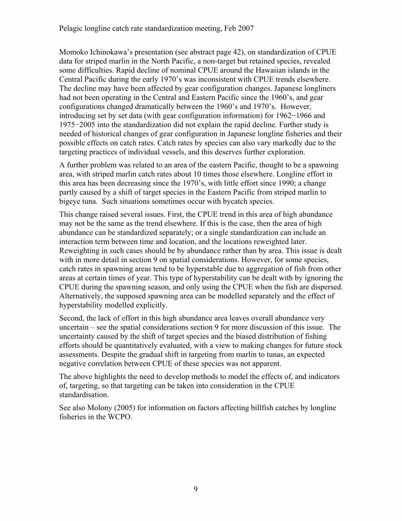
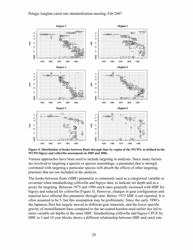
Targeting of particular species can affect catch rates in ways that are difficult to model if the target species is not identified. Simon Hoyle presented a discussion of targeting (see abstract page 47). The Japanese longline fleet has changed its targeting practises through time, with widespread increases in HBF since the 1970’s (Figure 4) paralleled by increases in the proportion of bigeye in the overall catch, particularly in regions 3 and 4 (see Figure 6 for a map of the regions). Other fleets have also seen adjustments in average targeting. A range of factors provide motivation for targeting particular species, including price, relative abundance, contractual obligations of vessels, and the preferences and skill-sets of skippers and crews. It was suggested that some skippers use the first 500 hooks to target the species, and the remaining hooks to determine where the fish are moving to.
Practices that enable vessels to target particular species or groups of species include fishing in particular regions, seeking appropriate local environmental conditions, using particular gear configurations (including HBF), materials and bait types, and adjusting the time of set. Vessels may target different species depending on moon phase, and there may be interactions between HBF and time of day, and time of day and moon phase. This emphasises the need for operational data.
19
Pelagic longline catch rate standardization meeting, Feb 2007
Figure 4: Distribution of hooks between floats through time by region of the WCPO, as defined in the WCPO bigeye and yellowfin assessments in 2005 and 2006.
Various approaches have been used to include targeting in analyses. Since many factors are involved in targeting a species or species assemblage, a parameter that is strongly correlated with targeting a particular species will absorb the effects of other targeting practises that are not included in the analysis.
The hooks between floats (HBF) parameter is commonly used as a categorical variable or covariate when standardizing yellowfin and bigeye data, to indicate set depth and as a proxy for targeting. Between 1975 and 1990 catch rates generally increased with HBF for bigeye and reduced for yellowfin (Figure 5). However, changes in gear configuration and material have affected this parameter through time. Before 1975 HBF is not reported. It is often assumed to be 5, but this assumption may be problematic. Since the early 1990’s the Japanese fleet has largely moved to different gear materials, and the lower specific gravity of monofilament lines compared to the tar-coated kuralon used earlier has led to more variable set depths at the same HBF. Standardizing yellowfin and bigeye CPUE by HBF in 5 and 10 year blocks shows a different relationship between HBF and catch rate
20
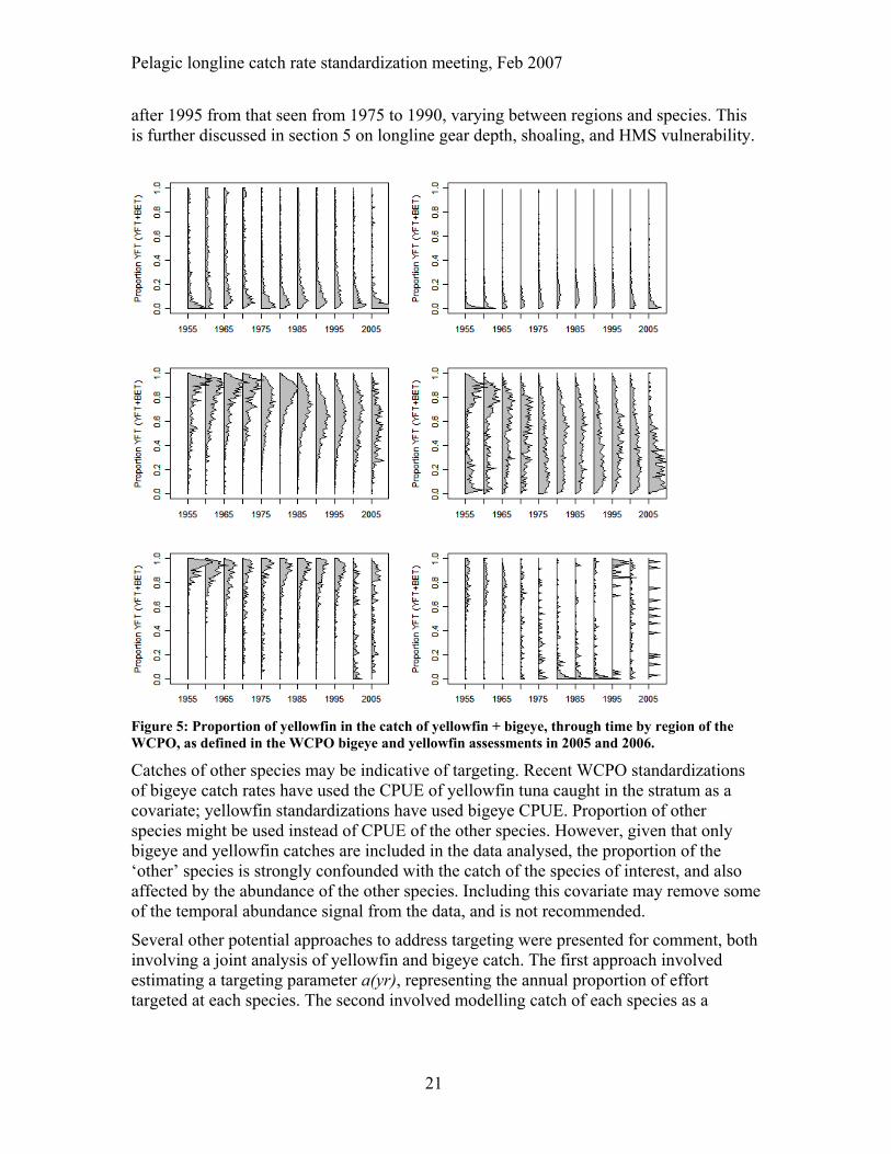
Pelagic longline catch rate standardization meeting, Feb 2007
after 1995 from that seen from 1975 to 1990, varying between regions and species. This is further discussed in section 5 on longline gear depth, shoaling, and HMS vulnerability.
Figure 5: Proportion of yellowfin in the catch of yellowfin + bigeye, through time by region of the WCPO, as defined in the WCPO bigeye and yellowfin assessments in 2005 and 2006.
Catches of other species may be indicative of targeting. Recent WCPO standardizations of bigeye catch rates have used the CPUE of yellowfin tuna caught in the stratum as a covariate; yellowfin standardizations have used bigeye CPUE. Proportion of other species might be used instead of CPUE of the other species. However, given that only bigeye and yellowfin catches are included in the data analysed, the proportion of the ‘other’ species is strongly confounded with the catch of the species of interest, and also affected by the abundance of the other species. Including this covariate may remove some of the temporal abundance signal from the data, and is not recommended.
Several other potential approaches to address targeting were presented for comment, both involving a joint analysis of yellowfin and bigeye catch. The first approach involved estimating a targeting parameter a(yr), representing the annual proportion of effort targeted at each species. The second involved modelling catch of each species as a
21

Pelagic longline catch rate standardization meeting, Feb 2007
function of the observed CPUE of the other species, offset by the predicted CPUE of the other species.
εγβ +⎟⎟⎠
⎞⎜⎜⎝
⎛⋅+⋅+
)()(log)log(~)log( 21 predBET
obsBETvariableseffortyft
εγβ +⎟⎟⎠
⎞⎜⎜⎝
⎛⋅+⋅+
)()(log)log(~)log( 22 predYFT
obsYFTvariableseffortbet
This approach is intended to identify strata where targeting was greater than predicted by the explanatory variables. However, this may be confounded because the other variables (HBF, area, time of year) also predict targeting. An alternative method used by Maunder and Hoyle (2006) for purse seine CPUE data is to include the known abundance of the other species based on stock assessment results. However, this approach does not take into account variation in the expected catch rate of the other species given the latitude, HBF, and other explanatory variables, and must be calibrated for the size selectivity of the longline gear, which can change in space and time.
The methods described above use the alternative target species, but using bycatch and minor species may also be appropriate. However, bycatch and minor species are not always reported, and are not currently available for the aggregated Japanese longline dataset, which reports only yellowfin, bigeye, and albacore. It is possible that presence-absence theory (e.g. MacKenzie et al. 2003) could be used to determine targeting of longline gear based on multiple species information. This approach may require set by set information and use consecutive sets as multiple samples of presence-absence.
Given set by set data, targeting could also be examined on a vessel basis, because it is unlikely that consecutive sets by the same vessel will be targeting different species. The species composition from individual longline sets could also be used in a statistical clustering approach to identify effort of different targeting types.
Such alternative methods of determining targeting are needed because some fleets do not report targeting or gear configuration. This is particularly important because the spatial area and fishing effort of the Japanese fleet are reducing as their fleet size reduces.
5. Longline gear depth, shoaling and HMS vulnerability
Gear configuration influences the depth at which the gear fishes. Some of the major operational factors that influence hook depth are:
• length of branch line • length of float line • catenary angle • distance between hooks • composition of the gear • line setting speed • hooks between floats
22
Pelagic longline catch rate standardization meeting, Feb 2007
However, of these factors only hooks between floats (HBF) is reported in the summarized Japanese longline data currently used for bigeye and yellowfin CPUE indices. Given the observed recent changes in the effect of HBF on catch rate (see targeting, section 3), investigation is needed of the relationships between gear characteristics, HBF, fishing depth, and catch rates.
The type and quality of information recorded in Japanese longline fishery logbooks have changed through time. The new distant water Japanese longline fishery logbook records information about gear, such as length of float line, length of branch lines, material, etc. However, there are some problems, e.g. there are three material codes on the logbook, but 10 different materials are in use and the consistency with which these are recorded is unknown.
HBF and catenary maximum fishing depth estimates should be used with caution in CPUE standardization. Environmental factors such as current surface velocity, current shear, and wind stress can also influence the depth that the gear fishes. Swordfish and tuna gear in the Hawaiian longline fishery were found to reach only about 50% and 70% respectively of the depth expected from a catenary algorithm (Bigelow presentation, BP6, see abstract page 48). Research in the very dynamic Windward Passage in the Caribbean found a large amount of variation in shoaling between and within shallowly deployed sets (Goodyear presentation, see abstract page 49). In some cases the deepest hook was at similar depths to the shallowest hook. The modes of the distributions for deep and shallow hooks were the same. However, given the high currents where this research was carried out, results may not necessarily apply to the tuna fleets. The gear was also different than that used by the tuna fleets.
Hook depth observations collected during monitored longline fishing experiments in the central South Pacific (Bach and Gaertner presentation, see abstract page 48) also showed that shoaling (absolute and relative) can be affected by current shear, set direction, and the shape of the mainline (i.e., the tangential angle), which is the strongest and the most consistent predictor in GLMs. HBF is the explanatory variable most frequently used to relate hook depth to preferred feeding depth of the species being analyzed. However, there are many problems with using HBF. These include interactions between area and HBF effect, and between quarter and HBF effect.
The recent change to 20 HBF may not have increased hook depth because it is associated with a change in the longline material to monofilament, which is more buoyant than the older material. Longline depths are therefore more variable now than previously, and depth can be adjusted by other methods such as with weights attached to the line.
Shoaling may also change during a set, with hooks initially at their maximum, but reducing in depth partway through the set. A captured fish can also shoal the longline.
Latitude and longitude often explain more catch rate variation than HBF. When latitude and longitude are used in the statHBS model, the habitat preference often becomes constant. This implies that the environmental variables averaged over the spatial and temporal strata used in the standardization are fairly constant over time. Spatial changes in the relationship of HBF and catch rate should be investigated.
23
Pelagic longline catch rate standardization meeting, Feb 2007
A software package named COPAL was presented by Pascal Bach (see abstract page 50) and is a tool designed for fishermen and scientists that estimates the underwater configuration of the fishing gear from set characteristics and drift speed of the mainline, based on catenary algorithms.
Further information on pelagic longline gear depth and shoaling can be found in Bigelow et al (2006).
6. Longline CPUE simulations
It is very important that methods used to standardize CPUE are tested, using simulation, to determine how well they perform, and in which situations the results can be validated. Phil Goodyear (see abstracts page 51) presented results of some analyses of simulated longline CPUE data, generated for blue marlin in the Atlantic. Initial analyses using this relatively realistic simulator showed that for this application, all the methods applied performed poorly.
Realistic simulators are good for evaluating the performance of methods, but it is often difficult to identify the reason why a method fails. It can also be useful to start with simple simulators and then add complexity, to determine which factors cause the problems. In the Atlantic blue marlin example, changes in the spatial effort distribution and/or gear configurations probably caused the methods to fail. However, more simulation work is needed to verify this. It is unlikely that the statHBS model will improve the analysis if the detHBS does not work with known habitat preference.
The simulation analyses showed some interesting characteristics. For example, even with constant ‘true’ abundance the CPUE declined, presumably due to changes in gear configuration. It was also interesting to note that the standardized CPUE was not very different from nominal CPUE. Something similar occurs in many applications, including standardization of bigeye CPUE in the WCPO, for which the standardized abundance indicator is similar to the trend from nominal CPUE despite changes in targeting and set depth, and inclusion of HBF in the standardization. This aspect of the standardization is important and deserves further investigation.
The poor relationship between some simulated abundance and CPUE data, even when standardized, suggests that, in some cases, using the index of abundance in the stock assessment will lead to misleading results, possibly with false precision. Since information quality is often poor about early parts of the fishery, it may be appropriate to focus on a more recent period than to include the historical CPUE data. Given estimates of recruitment, assumptions about the stock recruitment relationship, and information on depletion level from length frequency data, comparisons can be made with the biomass that would be available if there was no fishing. In analyses for the WCPO, most of the important management parameters are insensitive to data from before 1975. The early length frequency data are useful however for estimating asymptotic length. There are also well-established / entrenched reference points that require historical benchmarks.
In many analyses, CPUE standardization has little influence on the year effect compared to nominal values. Does this mean that nominal CPUE is generally good for longlines, so
24

Pelagic longline catch rate standardization meeting, Feb 2007
we don’t need to collect additional data, or is it because we don’t have the right covariates? Given the results of the longline CPUE simulations, the latter hypothesis seems more likely.
7. Time-series changes in catchability: Quantifying technological improvements
WCPFC stock assessments assume that longline catchability remains constant after standardizing for area and HBF, although this cannot be true. Many factors have influenced catchability through time. Longliners are motivated to upgrade their fishing gear and practices to improve fishing power and increase catchability. Ward and Myers (see abstract page 52) review technological changes in the fishery, which are largely likely to have increased catchability of target species.
These include electronic devices that facilitate navigation, communication and finding target species. Synthetic materials for lines and hooks have increased the probability of hooking and landing target species. Other changes have improved search efficiency (e.g., satellite imagery) or increased the proportion of time spent on fishing grounds (e.g., freezers). The number of hooks deployed daily has steadily increased since 1950, but without changing average soak time, as faster longline retrieval and deployment have balanced the increased hook numbers. All baits were once available at dawn; now more are available at dusk and at night. In the 1970s, several longline fleets began to exploit a much greater depth range, resulting in increased catchability for deep-dwelling species (e.g., bigeye tuna) and reduced catchability for epipelagic species like blue marlin. Recent bycatch mitigation measures have affected fishing power and catchability. Progressive improvements in expertise and technological improvements in the gear will also have affected fishing power, but are particularly difficult to quantify. New technologies that are effective are quickly taken up by all vessels, making them difficult to standardize out even if usage information were available. It is dangerous to rely on commercial data without also having fishery independent surveys or other means of calibrating the time-series.
The possibility of changes that may have reduced catchability was also discussed. Price signals from the market have changed through time, and fish quality may now be more important than previously, compared to the number of fish caught. Fish quality varies among areas, and better quality fish with higher fat content are generally found in cooler water. Thus the areas fished may have changed, and overall catch rates reduced. This change should be partly taken into account by the current practice of including 5º square as a categorical variable in the model, but there may be a need to further examine this issue by including a seasonal interaction.
The experience of skippers and crews is important given, for example, the need to understand oceanic currents. The economic strength of the Japanese longline fishery has declined since the 1980’s. In the early 1950’s and 1960’s the fishery, which began with demobilized navies, was very important both economically and culturally, and crews were of high quality. Vessels operated in groups and shared information. Fleets have now shrunk, so information sharing is less effective. Since the 1990’s there have been fewer Japanese crew on the vessels which may have reduced catchability.
25

Pelagic longline catch rate standardization meeting, Feb 2007
Technological changes that substantially improve catchability are likely to have been introduced rapidly across all fisheries and ocean basins. It would be useful to look for gear introduction effects by examining CPUE indices for similar species across all oceans.
For additional information on gear technology and factors likely to affect catch rates, see a summary of sources in Itano (2006), and also Itano (2004), Millar and Schneiter (2004), Swenarton and Beverley (2004), and Campbell and Young (2006).
8. Regional weighting
Regional weighting is highly influential in determining the status of yellowfin and bigeye in the WCPO (Hoyle presentation, see abstract page 53). The current weighting method uses a simplified version of the CPUE standardization model with data from 1960 to 1986 and in areas with HBF data and significant catch. There are a number of assumptions inherent in this approach, including that HBF has the same effect across all regions, and that the pre-1975 HBF is assumed to be five and consistent across regions.
The discussion converged with the earlier discussion on internal weighting of the regional abundance indices. Regions are standardized separately because their abundance trends differ, but there is also important variation in the abundance trend within regions. An appropriate response to this is to weight spatially by abundance. The current method of weighting by area is good for stable, well mixed stocks, but if there is significant interaction between area and time it can be misleading. Trends in CPUE by 5º square in the WCPO have been consistent within the main regions fished (Langley 2006b). Weighting by abundance can be done by estimating a separate abundance trend for each 5º square, and summing the results to give overall abundance.
A major constraint that has prevented weighting by abundance across the whole WCPO is that current software (R GLM) and computer memory do not permit such large analyses. There is a newly developed R package named biglm which is designed to be memory efficient and to analyze data in batches, for carrying out very large analyses. However, some problems have been encountered with its use. Alternatively, SAS could be used for standardization, because it may be more memory-efficient than R. Purpose-built AD Model Builder programs could also be used to fit large models.
9. Spatial considerations
Spatial variation occurs, at multiple spatial and temporal scales, in the distribution of both fish and fishing effort. Adam Langley (see abstract page 53) presented analyses of several related issues. The exclusion of the Japanese longline fleet from the domestic waters of Pacific Island countries/territories following the declaration of their EEZs would have biased assessments if the CPUE trends had been different inside and outside these zones. However, there was no apparent difference in CPUE indices, prior to the closures, within and outside these zones.
26

Pelagic longline catch rate standardization meeting, Feb 2007
The analysis highlighted both a spatial contraction of fishing effort and a shift toward the spatial cells with the highest bigeye CPUE (away from cells with high yellowfin CPUE). Thus from the mid-1980s the abundance index is increasingly driven by CPUE in the core bigeye cells, and there are limited data regarding changes in abundance beyond these cells. Further analysis indicates that, for yellowfin at least, the decline in CPUE is greater in the higher abundance cells than in the lower abundance cells. This indicates potential bias in the yellowfin CPUE index.
Addressing these biases may require the adoption of a more spatially-based approach to the CPUE analysis. Addressing variation in CPUE trend within the region will require weighting by abundance rather than by area. The current method, which includes 5º square in the standardization, weights by area within a region, and assumes that the ratios of abundances between areas remain constant through time. Given the lack of data from some areas, assumptions will need to be made regarding the level of CPUE in the cells where no (or very low) fishing occurred. Various plausible assumptions can be made about CPUE trends in unfished areas, so a sensitivity analysis approach may be required (e.g. Campbell 2004). See also Ahrens and Walters (2005).
One way to deal with unfished cells is to model abundance in them using a population dynamics model. Mark Maunder presented such an approach (see abstract page 54). The overall approach of combining the CPUE analysis with a population dynamics model has advantages beyond its utility for unfished cells, but also some disadvantages.
Unfished cells occur early in the fishery, as the fleet expands its spatial coverage; and during the fishery, as the stock status changes in different areas, and the operating conditions affecting fishery participants change. If each area is modelled as a separate population, and the CPUE standardization integrated with the population dynamics model, the population model can be used to estimate the abundance in years without data. A Pella-Tomlinson (PT) surplus production model can be used to model the population dynamics. Given the difficulty of estimating the parameters of the PT model from catch and effort data, particularly for areas with missing data, it would be advantageous to treat the parameters as random effects and share information among areas. The spatial correlation in parameters could be modelled using a spatial conditional autoregressive (CAR) model, and estimated using a frequentist (e.g. using ADMBre) or hierarchical Bayes framework using MCMC. A more complex model such as MULTIFAN-CL, which can incorporate other information (e.g. length frequency), and processes (e.g. movement between areas) may be more appropriate and effective, but is currently computationally infeasible.
Regional stratification of the WCPO was also discussed. Stock assessment models assume a homogeneous pool of fish. When modelling an area as large as the WCPO, the strong spatial variation in abundance trends is accommodated by dividing the area into regions and assessing them separately (Figure 6). Ideally the model would be run at a smaller spatial scale, but constraints include the time needed to run assessments, the spatial stratification of size sampling data, and the difficulty of estimating migration rates between regions. Assessment at a finer spatial scale over a short time period was suggested as a useful sensitivity analysis.
27

Pelagic longline catch rate standardization meeting, Feb 2007
30S
20S
10S
010
N20
N30
N
120E 140E 160E 180 160W 140W 120W 100W 80W
Legend0 3.5
Figure 6: Regional structure of the WCPO, coloured to show the relative catch per unit effort by 5º square between 1975 and 1986.
Previous analyses (Langley 2006a) have demonstrated justification for moving the northern boundary of regions 3 and 4 south by 10 degrees, for more homogeneous catch rates and size data. There is also an argument for splitting region 3 into two parts, because of the different size distributions and CPUE trends of these parts (Langley 2006b, 2006c), and the influential and unreliable catch data from the west of region 3. However, there are also sound administrative reasons for retaining the current structure, and a further disaggregated assessment is currently carried out as a sensitivity analysis. Disaggregating region 3 into two parts makes it difficult to assess the stock in the western part, although it is arguable that keeping the two parts together and assuming regional homogeneity reduces the accuracy and reliability of the overall assessment.
Alternative stock assessment stratifications could be based on oceanographic or biogeographical conditions, using Longhurst areas for example, although the 7-region version of the model (Langley 2006a) is a very close approximation to the Longhurst regions. CPUE data could be analyzed using regression trees and then simulated annealing used to partition the WCPO into regions of space with similar trends in CPUE (q.v. Watters and Deriso 2000), though this is a similar approach to that used by Langley (2006a), given the 10 x 20 degree spatial structure of the size data.
28
Pelagic longline catch rate standardization meeting, Feb 2007
10. Data: resolution, stratification, and data from other fleets (Korea, Taiwan, domestic)
Most analyses to estimate indices of abundance use data stratified by 5º square by month. However, some data are available in finer detail. For example, set by set data are available for commercial gear, and some hook by hook research data are available. These more detailed data provide potential benefits over stratified data, and requires investigation. For example, the set by set data contain more covariates (e.g. vessel, skipper, bait type, gear material, time of set) and can be associated with more environmental data (e.g. moon phase); factors that may explain variation in CPUE which could otherwise bias the year effect.
Momoko Ichinokawa’s presentation (Ichinokawa and Yokawa 2006; see abstract page 42) was notable for its use of set by set Japanese longline data. Ichinokawa and Yokawa’s preliminary analyses have focused on spatial and seasonal variation in CPUE and its relationship with HPB.
Work is under way at the National Institute of Far Seas Fisheries to recover set by set longline data, which is of variable quality, both through time as logbooks change, and between vessels and skippers. Only major species are reported in the early period. The data contain no information on time of set. Gear material, length of branch line, and length of float line are recorded once per month, although length of float line is likely to have changed more frequently than this.
The meeting encouraged this data recovery work and noted the great potential of these data for improving indices of abundance and stock assessments. Catch rates are heterogeneous within the aggregations currently used, and the detailed data are likely to be informative about the characteristics that lead to this heterogeneity.
It was noted that fishing at randomly selected set locations often produced no fish. This reinforces the potential importance of effects not included in models using aggregated data, such as skipper experience and ability. It also suggests that fishery independent surveys are not practical.
Several sources of set-by-set longline data are currently available for the WCPO. These are the in-country data held by the SPC from distant water fishing nations (principally Japan, Korea, Taiwan) fishing within the EEZs of Pacific states. In addition there are observer data for five to six 5º squares around Fiji over a 10 year period. These data could be used to examine assumptions and methodologies, and to estimate indices of abundance for comparison with those currently used.
The availability of Japanese set by set longline data is currently constrained by the needs to carefully prepare and validate the data, and to ensure that the complexity of the changing logbooks and data quality issues are understood by analysts. Until these data are better understood and described, collaborative projects with Japanese scientists will be the most useful approach.
Standardizing longline data at a 1º rather than 5º scale can be advantageous, but this depends on the methods used. Standardizing Japanese longline data for the WCPO aggregated at 1º and 5º using a model that include quarter, HBF, and 5º area found no difference in the year effect. However, targeting may occur at the 1º scale, a scale
29

Pelagic longline catch rate standardization meeting, Feb 2007
important for southern bluefin tuna, so it is important to consider how this might affect analyses.
As noted earlier, since the early 1990’s the Japanese fleet has largely moved to different gear materials, and the lower specific gravity of monofilament lines compared to the tar-coated kuralon used earlier has led to more variable set depths at the same HBF. Additional stratification of the Japanese longline data provided to RFMO’s would be useful, particularly given the apparent importance of the post-1993 change in gear material and its specific gravity.
Given the progressive and ongoing reduction of the Japanese longline fleet, and the contraction of its area of operation, there is a need to make greater use of data from other fleets, particularly the relatively long time series available from the Korean and Chinese Taipei longline fleets. It would be useful to compare the abundance indices and other parameters derived by area and period. For example, the Korean longline fleet have wide spatial coverage, and would make an interesting comparison with the Japanese longline data, given their different targeting practises. There are some concerns about data quality that need to be considered, such as the lack of gear information and observer coverage, but the Korean fleet generally uses 5 to 8 HBF.
One possible approach would be to use a cluster analysis on the species composition of the catches to identify the target species (He et al. 1997). This approach would not be appropriate for aggregated data, since targeting occurs at the set level. The approach could be applied to within-country Japanese and Korean logsheet data held by SPC. It is unlikely to be applicable to Taiwanese data, which generally reports only albacore and bigeye. Comparison of indices from different fleets, and the clusters within the fleets, may be highly informative.
One possible difference between fleets is their setting practises, which may lead to different catchabilities. For example, there is anecdotal evidence of some Korean and/or Taiwanese vessels setting twice per day, up to 5000 hooks per day. These vessels carry double crews, and may set and haul at the same time. It will be important to establish an observer program, and/or obtain descriptions of the fisheries from national scientists, in order to understand the fishing practises.
30

Pelagic longline catch rate standardization meeting, Feb 2007
References
Ahrens R. and Walters, C. (2005). Why are there still large pelagic predators in the oceans?: evidence of severe hyper-depletion in longline catch-per-effort. WCPFC-SC1, ME-WP-3. 13 pp.
Bach, P. and Fonteneau, A. (2005). Historical shifts in hooks between floats and potential target species of the Japanese longline fishery in the equatorial Western Indian Ocean. IOTC-2005-SC-INFO16.
Bach, P., Travassos, P. and Gaertner, D. (2006). Why the number of hooks per basket (HPB) is not a good proxy indicator of the maximum fishing depth in drifting longline fisheries? Col. Vol. Sci. Pap. ICCAT, 59(2): 701-715.
Besag, J.E. 1974. Spatial interaction and the statistical analysis of lattice systems. Journal of the Royal Statistical Society, Series B 36: 192-236.
Bigelow, K.A., Maunder, M.N. and Hinton, M. (2003) Comparison of deterministic and statistical habitat-based models to estimate effective longline effort and standardized CPUE for bigeye and yellowfin tuna. SCTB16 RG-3.
Bigelow, K., Musyl, M.K., Poisson, F. and Kleiber, P. (2006) Pelagic longline gear depth and shoaling. Fisheries Research 77:173-18.
Campbell, R.A. (2004). CPUE standardisation and the construction of indices of stock abundance in a spatially varying fishery using general linear models. Fisheries Research 70(2-3): 209-227.
Campbell, R. and Young, J. (2006). Measuring effective longline effort in the Australian Eastern Tuna and Billfish Fishery. WCPFC-SC2, FTWP-2, 22 pp.
Cressie N. 1993. Statistics for Spatial Data, Revised Edition. New York: John Wiley and Sons.
Goodyear, C.P. (2006). Performance diagnostics for the longline CPUE simulator. Col. Vol. Sci. Pap. ICCAT, 59(2): 615-626.
Goodyear, C.P. (2006). Simulated Japanese longline CPUE for blue marlin and white marlin. Col. Vol. Sci. Pap. ICCAT, 59(1): 211-223.
Haining R. 1990. Spatial Data Analysis in the Social and Environmental Sciences. Cambridge: Cambridge University Press.
He, X., Bigelow, K.A., and Boggs, C.H. (1997) Cluster analysis of longline sets and fishing strategies within the Hawaii-based fishery. Fisheries Research 31:147–158.
Hinton, M. G., Bayliff, W.H. and Suter, J. 2005. Assessment of swordfish in the eastern Pacific Ocean. Inter-Amer. Trop. Tuna Comm. Stock Assess. Rpt. 5, 291:326.
Hinton, M.G. and Maunder, M.N. (2003). Methods of standardizing CPUE and how to select among them. SCTB 16, MWG-7, 13 pp.
31
Pelagic longline catch rate standardization meeting, Feb 2007
Hinton, M. G. and Nakano, H. 1996. Standardizing catch and effort statistics using physiological, ecological, or behavioural constraints and environmental data, with an application to blue marlin (Makaira nigricans) catch and effort data from the Japanese longline fisheries in the Pacific. Inter-American Tropical Tuna Commission Bulletin 21: 171–200.
Hoyle, S.D. and Maunder M.N. (2006) Standardisation of yellowfin and bigeye CPUE data from Japanese longliners, 1975-2004. IATTC Working Group on Stock Assessments, 6th Meeting, SAR-7-07. (http://www.iattc.org/PDFFiles2/SAR-7-07-LL-CPUE-standardization.pdf)
Ichinokawa, M. Yokawa, K. (2006). Standardized CPUE of striped marlin caught by Japanese distant water longliners using set-by-set data in the north Pacific. ISC/06/MARLIN&SWO-WG, 25 pp.
Itano, D.G. (2004). Vessel and gear attributes useful for the long-term monitoring and management of WCPO tropical tuna fisheries. SCTB 17, FTWG–2, 14 pp.
Itano, D.G. (2006). An examination of vessel, gear and operational details useful for fishery-specific effort standardization, including FAD-related gear and fishing strategies. WCPFC SC2, FTWP-6, 9 pp.
Kieseppä, I.A. (2003). AIC and Large Samples. Philosophy of Science (East Lansing) 70: 1265-1276.
Kleiber, P. (2002). Standardizing longline fishing effort in stock assessment models: effect of oceanic conditions. SCTB15, MWG-4. 3 pp.
Konishi, S. and Kitagawa, G. (1996). Generalised information criteria in model selection. Biometrika 83: 875-890.
Knight, E., Park, T., Bromhead, D., Ward, P., Barry, S. and Summerson, R. (2006) Analyses of interactions between longline and recreational gamefish fisheries taking or tagging striped marlin off New South Wales. Bureau of Rural Sciences. Canberra.
Langley, A.D. (2004). An examination of the influence of recent oceanographic conditions on the catch rate of albacore in the main domestic longline fisheries. SCTB 17, SA-4, 25 pp.
Langley, A. 2006a. Summary report from yellowfin and bigeye stock assessment workshop. ME WP-1, WCPFC-SC2, Manila, Philippines, 7−18 August 2006.
Langley, A. 2006b. Spatial and temporal trends in yellowfin and bigeye longline CPUE for the Japanese fleet in the WCPO. WCPFC-SC2, ME IP-1, Manila, Philippines, 7−18 August 2006.
Langley, A. 2006c. Spatial and temporal variation in the size composition of the yellowfin and bigeye longline catch in the WCPO. ME IP-2, WCPFC-SC2, Manila, Philippines, 7−18 August 2006.
Langley, A., Bigelow, K. Maunder, M.N. and Miyabe, N. (2005) Longline CPUE indices for bigeye and yellowfin in the Pacific Ocean using GLM and statistical habitat standardisation methods. WCPFC–SC1, SA WP–8, 40pp.
32
Pelagic longline catch rate standardization meeting, Feb 2007
Little, R., and Rubin, D. 1987. Statistical analysis with missing data. John Wiley and Sons, New York, 278 pp.
Maunder M.N. (2001) A general framework for integrating the standardization of catch-per-unit-of-effort into stock assessment models. Can. J. Fish. Aquat. Sci., 58: 795-803.
Maunder, M.N. and Hinton, M.G. (2006) Estimating relative abundance from catch and effort data, using neural networks. Inter-American Tropical Tuna Commission Special Report 15. pp. 19. (http://www.iattc.org/PDFFiles2/Special-Report-15-Neural-Networks.pdf)
Maunder, M.N., Hinton, M.G., Bigelow, K.A. and Harley, S.J. (2002) Statistical comparisons of habitat standardised effort and nominal effort, SCTB 15, MWG-7, 18p.
Maunder, M.N., Hinton, M.G., Bigelow, K.A. Langley, A.D. (2006) Developing indices of abundance using habitat data in a statistical framework. Bulletin of Marine Science, 79(3): 545–559.
Maunder, M.N. and Hoyle, S.D. (2007) Analysis of skipjack catch per unit of effort (CPUE). IATTC Working Group on Stock Assessments, 6th Meeting, SAR-7-07b (http://www.iattc.org/PDFFiles2/SAR-7-07b-SKJ-CPUE-analysis.pdf)
Maunder, M.N. and Langley, A.D. (2004) Integrating the standardization of catch-per-unit-of-effort into stock assessment models: testing a population dynamics model and using multiple data types. Fisheries Research 70(2-3): 389-395.
MacKenzie, D.I., Nichols, J.D., Hines, J.D., Knutson, M.G. and Franklin, A.B. (2003). Estimating site occupancy, colonization, and local extinction when a species is detected imperfectly. Ecology 84(8): 2200-2207.
Millar, C. and Schneiter, E. (2004). Review of vessel and gear attribute data held by SPC and FFA. SCTB 17, FTWG-1.
Minami, M., Lennert-Cody, C.E., Gaoc, W. and Roman-Verdesoto, M. (2007). Modeling shark bycatch: The zero-inflated negative binomial regression model with smoothing. Fisheries Research 84: 210-221.
Molony, B. (2005). Summary of the biology, ecology and stock status of billfishes in the WCPFC, with a review of major variables influencing longline fishery performance. WCPFC SC1, EB-WP2. 67 pp.
Shono, H. (2005). Is model selection using Akaike's information criterion appropriate for catch per unit effort standardization in large samples? Fisheries Science, 71: 978-986.
Swenarton, T. and Beverly, S. (2004). Documentation and classification of fishing gear and technology on board pelagic longline vessels: Hawaii module. SCTB 17, INF-FTWG-2, 17 pp.
W. N. Venables and B. D. Ripley. (2002). Modern Applied Statistics with S. Springer.
Walsh, W.A., Howell, E.A., Bigelow, K.A. and McCracken, M.L. (2006). Analyses of observed longline catches of blue marlin, Makaira nigricans, using generalized additive models with operational and environmental predictors. Bulletin of Marine Science, 79(3): 607–622. (BP3)
33
Pelagic longline catch rate standardization meeting, Feb 2007
Ward, P. and Myers, R.A. (2005). A method for inferring the depth distribution of catchability for pelagic fishes and correcting for variations in the depth of longline fishing gear. Canadian Journal of Fisheries and Aquatic Sciences 62(5): 1130–1142.
Ward, P., Myers, R.A. and Blanchard, W. (2004). Fish lost at sea: The effect of soak time and timing on pelagic longline catches. Fishery Bulletin 102: 179–195.
Walters, C. (2003). Folly and fantasy in the analysis of spatial catch rate data. Can. J. Fish. Aquat. Sci. 60(12), 1433-1436.
Watters, G. and Deriso, R. (2000). Catch per unit of effort of bigeye tuna: a new analysis with regression trees and simulated annealing. Bulletin of the Inter American Tropical Tuna Commission, 21(8), 527–571.
Yokawa K., Saito, H., Kanaiwa, M. and Takeuchi, Y. (2006). Vertical distribution pattern of CPUE of Atlantic billfishes and associated species estimated using longline research data. Bulletin of Marine Science, 79(3), 623-634.
34
Pelagic longline catch rate standardization meeting, Feb 2007
Appendix I: Agenda
Pelagic Longline Catch Rate Standardizations February 12−16, 2007
Imin Conference Center University of Hawaii, Honolulu
10:30 a.m. Monday, February 12th 9 a.m. Tuesday-Friday, February 13-16
th
Opening John Sibert 1. Introductions Simon Hoyle/Keith Bigelow 2. Overview of longline effort standardizations in current Pacific HMS assessments
A. Western and central Pacific Ocean tunas Adam Langley
Longline CPUE indices for bigeye and yellowfin in the Pacific Ocean using GLM and statistical habitat standardisation methods (BP1).
B. Eastern Pacific Ocean tunas Simon Hoyle/Mark Maunder
Standardization of yellowfin and bigeye CPUE data from Japanese longliners, 1975−2004 (BP2)
C. Standardization of striped marlin caught by Japanese longliners in the North Pacific Momoko Ichinokawa/Kotaro Yokawa
3. Models for standardizing longline effort
A. Generalized Linear (GLMs), Generalized Additive Models (GAMs) and Neural Networks − covariates, oceanographic and otherwise (e.g. albacore data)
Oceanographic influences on CPUE Adam Langley
Aspects of model selection for GLMs applied to striped marlin in the Hawaii-based longline fishery (WP1) Jon Brodziak
Analyses of Observed Longline Catches of Blue Marlin , Makaira nigricans, using GAMs with Operational and Environmental Predictors (BP3) Keith Bigelow
B. Standardization models with depth-related vulnerability
35

Pelagic longline catch rate standardization meeting, Feb 2007
A method for inferring the depth distribution of catchability for pelagic fishes and correcting for variations in the depth of longline fishing gear (BP4) Peter Ward
C. Standardization models with habitat-related vulnerability (statHBS)
Developing indices of abundance using habitat data in a statistical framework (BP5) Mark Maunder
Using statHBS with a multiple species approach (WP) Minoru Kanaiwa
Does habitat or depth influence catch rates of pelagic species? Keith Bigelow/Mark Maunder
4. Targeting
Hooks between floats and Japanese longline data. Simon Hoyle/Adam Langley
Joint analysis of YFT and BET CPUE from Japanese longline data. Simon Hoyle/Adam Langley
Using hooks between floats as a proxy for maximum fishing depth (BP7, BP8) Pascal Bach/Daniel Gaertner
5. Longline gear depth, shoaling and HMS vulnerability
Pelagic longline gear depth and shoaling (BP6) Keith Bigelow
Pelagic longline fishing depth: Confronting catenary theory data with depth observations from monitored longline fishing experiments (WP5) Pascal Bach/Daniel Gaertner
Recent topics of tuna longline CPUE analysis within the National Research Institute of Far Seas Fisheries Kotaro Yokawa
Longline observations and marlin vulnerability (WP2, WP3) Phil Goodyear
The COPAL software: a tool to estimate both hook depths and the maximum fishing depth of longlines according to setting tactic information Pascal Bach/Daniel Gaertner
6. Longline CPUE simulations (BP9, BP10) Phil Goodyear 7. Time-series changes in catchability: Quantifying technological improvements
An overview of historical changes in the fishing gear and practices of pelagic longliners (WP4) Peter Ward
8. Regional weighting Simon Hoyle 9. Spatial considerations Adam Langley
A. Focusing on ‘core’ areas and the effects on CPUE of EEZ declaration and subsequent exclusion
36

Pelagic longline catch rate standardization meeting, Feb 2007
B. Defining appropriate regional stratification for a spatially structured assessment model
C. Modelling at differing scales: individual longline sets, 1º and 5º data
Relative abundance trends of tuna and billfishes in the Pacific Ocean inferred from Japanese longline spatial catch and effort data (WP6) Robert Ahrens
spatial catch effort data
10. Utility of data from other fleets (Korea, Taiwan, domestic) (tentative) 11. Summarize recommendations for longline effort standardization for use in current stock assessments
37
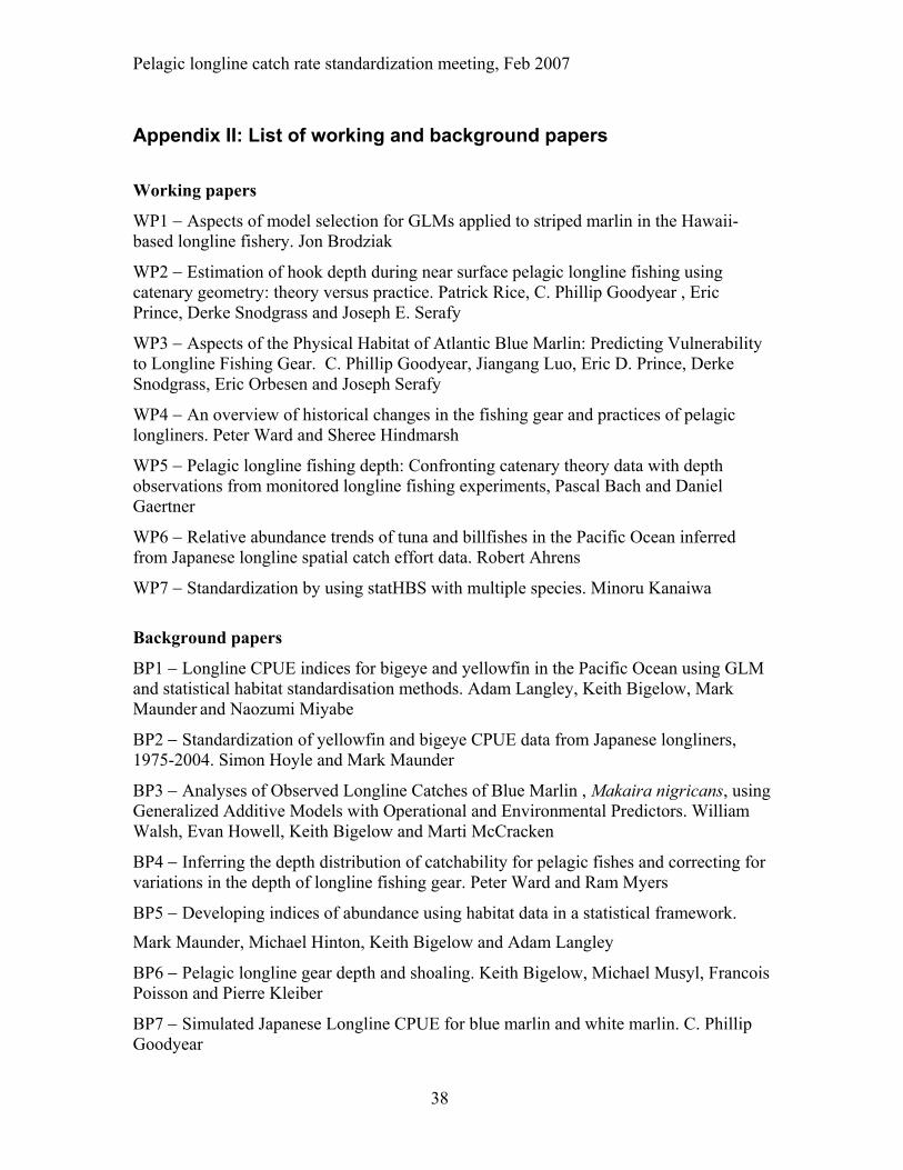
Pelagic longline catch rate standardization meeting, Feb 2007
Appendix II: List of working and background papers
Working papers
WP1 − Aspects of model selection for GLMs applied to striped marlin in the Hawaii-based longline fishery. Jon Brodziak
WP2 − Estimation of hook depth during near surface pelagic longline fishing using catenary geometry: theory versus practice. Patrick Rice, C. Phillip Goodyear , Eric Prince, Derke Snodgrass and Joseph E. Serafy
WP3 − Aspects of the Physical Habitat of Atlantic Blue Marlin: Predicting Vulnerability to Longline Fishing Gear. C. Phillip Goodyear, Jiangang Luo, Eric D. Prince, Derke Snodgrass, Eric Orbesen and Joseph Serafy
WP4 − An overview of historical changes in the fishing gear and practices of pelagic longliners. Peter Ward and Sheree Hindmarsh
WP5 − Pelagic longline fishing depth: Confronting catenary theory data with depth observations from monitored longline fishing experiments, Pascal Bach and Daniel Gaertner
WP6 − Relative abundance trends of tuna and billfishes in the Pacific Ocean inferred from Japanese longline spatial catch effort data. Robert Ahrens
WP7 − Standardization by using statHBS with multiple species. Minoru Kanaiwa
Background papers
BP1 − Longline CPUE indices for bigeye and yellowfin in the Pacific Ocean using GLM and statistical habitat standardisation methods. Adam Langley, Keith Bigelow, Mark Maunder
and Naozumi Miyabe
BP2 − Standardization of yellowfin and bigeye CPUE data from Japanese longliners, 1975-2004. Simon Hoyle and Mark Maunder
BP3 − Analyses of Observed Longline Catches of Blue Marlin , Makaira nigricans, using Generalized Additive Models with Operational and Environmental Predictors. William Walsh, Evan Howell, Keith Bigelow and Marti McCracken
BP4 − Inferring the depth distribution of catchability for pelagic fishes and correcting for variations in the depth of longline fishing gear. Peter Ward and Ram Myers
BP5 − Developing indices of abundance using habitat data in a statistical framework.
Mark Maunder, Michael Hinton, Keith Bigelow and Adam Langley
BP6 − Pelagic longline gear depth and shoaling. Keith Bigelow, Michael Musyl, Francois Poisson and Pierre Kleiber
BP7 − Simulated Japanese Longline CPUE for blue marlin and white marlin. C. Phillip Goodyear
38

Pelagic longline catch rate standardization meeting, Feb 2007
BP8 − Performance diagnostics for the longline CPUE simulator. C. Phillip Goodyear
BP9 − Historical shifts in hooks between floats and potential target species of the Japanese longline fishery in the equatorial Western Indian Ocean. Pascal Bach and Alain Fonteneau
BP10 − Why the number hooks per basket (HPB) is not a good proxy indicator of the maximum fishing depth in drifting longline fisheries? P. Bach, P. Travassos, D. Gaertner
39
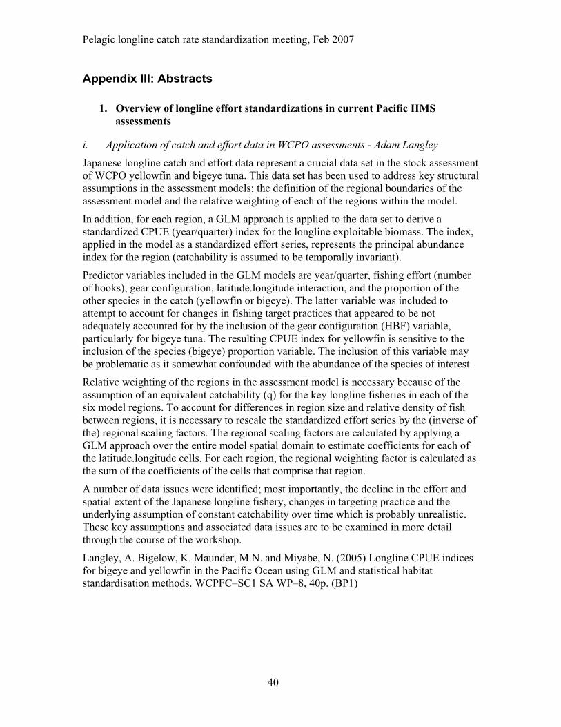
Pelagic longline catch rate standardization meeting, Feb 2007
Appendix III: Abstracts
1. Overview of longline effort standardizations in current Pacific HMS assessments
i. Application of catch and effort data in WCPO assessments - Adam Langley
Japanese longline catch and effort data represent a crucial data set in the stock assessment of WCPO yellowfin and bigeye tuna. This data set has been used to address key structural assumptions in the assessment models; the definition of the regional boundaries of the assessment model and the relative weighting of each of the regions within the model.
In addition, for each region, a GLM approach is applied to the data set to derive a standardized CPUE (year/quarter) index for the longline exploitable biomass. The index, applied in the model as a standardized effort series, represents the principal abundance index for the region (catchability is assumed to be temporally invariant).
Predictor variables included in the GLM models are year/quarter, fishing effort (number of hooks), gear configuration, latitude.longitude interaction, and the proportion of the other species in the catch (yellowfin or bigeye). The latter variable was included to attempt to account for changes in fishing target practices that appeared to be not adequately accounted for by the inclusion of the gear configuration (HBF) variable, particularly for bigeye tuna. The resulting CPUE index for yellowfin is sensitive to the inclusion of the species (bigeye) proportion variable. The inclusion of this variable may be problematic as it somewhat confounded with the abundance of the species of interest.
Relative weighting of the regions in the assessment model is necessary because of the assumption of an equivalent catchability (q) for the key longline fisheries in each of the six model regions. To account for differences in region size and relative density of fish between regions, it is necessary to rescale the standardized effort series by the (inverse of the) regional scaling factors. The regional scaling factors are calculated by applying a GLM approach over the entire model spatial domain to estimate coefficients for each of the latitude.longitude cells. For each region, the regional weighting factor is calculated as the sum of the coefficients of the cells that comprise that region.
A number of data issues were identified; most importantly, the decline in the effort and spatial extent of the Japanese longline fishery, changes in targeting practice and the underlying assumption of constant catchability over time which is probably unrealistic. These key assumptions and associated data issues are to be examined in more detail through the course of the workshop.
Langley, A. Bigelow, K. Maunder, M.N. and Miyabe, N. (2005) Longline CPUE indices for bigeye and yellowfin in the Pacific Ocean using GLM and statistical habitat standardisation methods. WCPFC–SC1 SA WP–8, 40p. (BP1)
40

Pelagic longline catch rate standardization meeting, Feb 2007
ii. Methods used to standardize longline catch and effort data in the EPO – Mark N. Maunder and Simon D. Hoyle.
The IATTC has developed and used several methods to standardize longline CPUE data to generate relative indices of abundance for use in stock assessment models. These methods include regression trees (Watters and Deriso 2000), habitat based standardization (HBS, Hinton and Nakano 1996), statistical habitat based standardization (statHBS, Maunder et al. 2006), neural networks (Maunder and Hinton 2006), GLMs (Hinton et al. 2005), and delta-log normal GLMs (Hoyle and Maunder 2006). The habitat based standardization approaches are based on the scientific understanding of how the longline fisheries operate and the interaction between fish, their habitat, and the gear. Regression trees and neural networks are nonparametric approaches that allow the data to estimate the relationship between CPUE and covariates rather than relying on the scientific understanding. The GLM approaches are more traditional and the delta-lognormal models explicitly model the zero catches. Oceanographic data have been included in GLMs as an alternative to the HBS methods. In general, the methods produce similar relative indices of abundance, except the deterministic habitat based standardization method. The explanatory variables used in the analyses generally do not impact the estimate of the relative index of abundance. A method developed for analyzing purse seine CPUE data that is based on the ratio of catch to that of a species for which abundance is known (e.g. from a stock assessment) may provide an alternative method for analyzing CPUE data, particularly for bycatch and minor species (Maunder and Hoyle 2006). Currently, the delta-lognormal GLM method with the explanatory variables hooks between floats and 5x5 degree square is used to develop indices of abundance. However, this is because there is currently no preferred method and all methods produce similar results.
Hinton, M. G., Bayliff, W.H. and J. Suter. 2005. Assessment of swordfish in the eastern Pacific Ocean. Inter-Amer. Trop. Tuna Comm. Stock Assess. Rpt. 5, 291:326.
Hinton M.G. and Nakano H. 1996. Standardizing catch and effort statistics using physiological, ecological, or behavioral constraints and environmental data, with an application to blue marlin (Makaira nigricans) catch and effort data from the Japanese longline fisheries in the Pacific. Inter-Am. Trop. Tuna Comm. Bull. 21: 171–200.
Hoyle, S.D. and Maunder M.N. (2006) Standardisation of yellowfin and bigeye CPUE data from Japanese longliners, 1975-2004. IATTC Working Group on Stock Assessments, 6th Meeting, SAR-7-07. (http://www.iattc.org/PDFFiles2/SAR-7-07-LL-CPUE-standardization.pdf) (BP2)
Maunder, M.N., Hinton, M.G., Bigelow, K.A. and Langley, A.D. (2006) Developing indices of abundance using habitat data in a statistical framework. Bulletin of Marine Science, 79(3): 545–559.
Maunder, M.N. and Hinton, M.G. (2006) Estimating relative abundance from catch and effort data, using neural networks. Inter-American Tropical Tuna Commission Special Report 15. pp. 19. (http://www.iattc.org/PDFFiles2/Special-Report-15-Neural-Networks.pdf)
41

Pelagic longline catch rate standardization meeting, Feb 2007
Maunder, M.N. and Hoyle, S.D. (2007) Analysis of skipjack catch per unit of effort (CPUE). IATTC Working Group on Stock Assessments, 6th Meeting, SAR-7-07b (http://www.iattc.org/PDFFiles2/SAR-7-07b-SKJ-CPUE-analysis.pdf)
Watters, G. and Deriso, R. (2000). Catch per unit of effort of bigeye tuna: a new analysis with regression trees and simulated annealing. Bull. Int. Am. Trop. Tuna Commun. 21 (8), 527–571.
iii. Standardized CPUE of striped marlin caught by Japanese distant water longliners in the North Pacific – Momoko Ichinokawa and Kotaro Yokawa
This presentation overviewed the Japanese longliners fishing for striped marlin (STM) in the North Pacific, and suggested major problems in standardizing CPUE of STM. The first problem is a rapid decline of nominal CPUE around Hawaii islands in the Central Pacific during early 1970’s. Because 1960’s was a very early period of Japanese longliners operating in the Central and Eastern Pacific, and gear configuration of the Japanese longliners drastically changed from 1960’s to 1970’s, possible changes of the gear configuration could cause a decline in STM CPUE However, the latest results of standardization of STM, using set-by-set data including information on gear configuration during 1962-1966 and 1975-2005, could not explain the rapid decline. Therefore, further study would be needed for investigating the historical change of gear configuration in Japanese longline fisheries, and its possible effects to the CPUE standardization. The second is a shift of targeting species from STM to bigeye tuna in the Eastern Pacific. Longline effort targeting STM at its spawning area in the Eastern Pacific has been decreasing since 1970’s, and rarely occurred since 1990. Because CPUE in the spawning area of STM is about 10 times larger than those in the other regions, it makes overall CPUE weighted by area very uncertain. Such a situation is sometimes observed in by-catch species. The uncertainty of CPUE caused from a shift of targeting species and biased distribution of fishing efforts should be quantitatively evaluated, and incorporated into stock assessment in a future study.
2. Models for standardizing longline effort: GLMs, GAMs, neural networks and covariates
iv. Incorporation of oceanographic data in the standardization of longline CPUE for the WCPO stock assessments – A. Langley
Previous reviews of longline CPUE standardizations have identified the potential importance of including oceanographic variables in the GLM models for yellowfin, bigeye and South Pacific albacore. Catch and effort data included in these models are available at a relatively broad spatial (5º lat/long) and temporal (monthly) scale. Oceanographic data, derived from physical-biogeochemical models, are also available at a comparable resolution. Both data sets represent average conditions over a relatively broad spatial/temporal scale and do not characterise the fine-scale heterogeneity that may exist in both the environment and fish distribution.
42
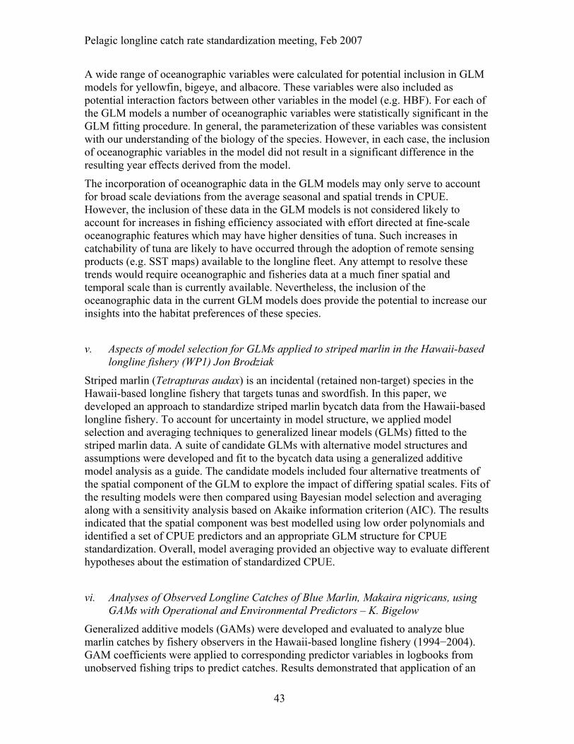
Pelagic longline catch rate standardization meeting, Feb 2007
A wide range of oceanographic variables were calculated for potential inclusion in GLM models for yellowfin, bigeye, and albacore. These variables were also included as potential interaction factors between other variables in the model (e.g. HBF). For each of the GLM models a number of oceanographic variables were statistically significant in the GLM fitting procedure. In general, the parameterization of these variables was consistent with our understanding of the biology of the species. However, in each case, the inclusion of oceanographic variables in the model did not result in a significant difference in the resulting year effects derived from the model.
The incorporation of oceanographic data in the GLM models may only serve to account for broad scale deviations from the average seasonal and spatial trends in CPUE. However, the inclusion of these data in the GLM models is not considered likely to account for increases in fishing efficiency associated with effort directed at fine-scale oceanographic features which may have higher densities of tuna. Such increases in catchability of tuna are likely to have occurred through the adoption of remote sensing products (e.g. SST maps) available to the longline fleet. Any attempt to resolve these trends would require oceanographic and fisheries data at a much finer spatial and temporal scale than is currently available. Nevertheless, the inclusion of the oceanographic data in the current GLM models does provide the potential to increase our insights into the habitat preferences of these species.
v. Aspects of model selection for GLMs applied to striped marlin in the Hawaii-based longline fishery (WP1) Jon Brodziak
Striped marlin (Tetrapturas audax) is an incidental (retained non-target) species in the Hawaii-based longline fishery that targets tunas and swordfish. In this paper, we developed an approach to standardize striped marlin bycatch data from the Hawaii-based longline fishery. To account for uncertainty in model structure, we applied model selection and averaging techniques to generalized linear models (GLMs) fitted to the striped marlin data. A suite of candidate GLMs with alternative model structures and assumptions were developed and fit to the bycatch data using a generalized additive model analysis as a guide. The candidate models included four alternative treatments of the spatial component of the GLM to explore the impact of differing spatial scales. Fits of the resulting models were then compared using Bayesian model selection and averaging along with a sensitivity analysis based on Akaike information criterion (AIC). The results indicated that the spatial component was best modelled using low order polynomials and identified a set of CPUE predictors and an appropriate GLM structure for CPUE standardization. Overall, model averaging provided an objective way to evaluate different hypotheses about the estimation of standardized CPUE.
vi. Analyses of Observed Longline Catches of Blue Marlin, Makaira nigricans, using GAMs with Operational and Environmental Predictors – K. Bigelow
Generalized additive models (GAMs) were developed and evaluated to analyze blue marlin catches by fishery observers in the Hawaii-based longline fishery (1994−2004). GAM coefficients were applied to corresponding predictor variables in logbooks from unobserved fishing trips to predict catches. Results demonstrated that application of an
43
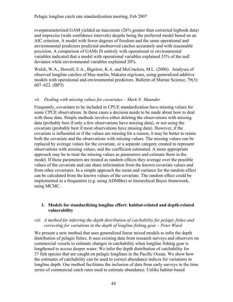
Pelagic longline catch rate standardization meeting, Feb 2007
overparameterized GAM yielded an inaccurate (26% greater than corrected logbook data) and imprecise (wide confidence intervals) despite being the preferred model based on an AIC criterion. A model with fewer degrees of freedom and the same operational and environmental predictors predicted unobserved catches accurately and with reasonable precision. A comparison of GAMs fit entirely with operational or environmental variables indicated that a model with operational variables explained 33% of the null deviance while environmental variables explained 20%.
Walsh, W.A., Howell, E.A., Bigelow, K.A. and McCracken, M.L. (2006). Analyses of observed longline catches of blue marlin, Makaira nigricans, using generalized additive models with operational and environmental predictors. Bulletin of Marine Science, 79(3): 607–622. (BP3)
vii. Dealing with missing values for covariates – Mark N. Maunder
Frequently, covariates to be included in CPUE standardization have missing values for some CPUE observations. In these cases a decision needs to be made about how to deal with these data. Simple methods involve either deleting the observations with missing data (probably best if only a few observations have missing data), or not using the covariate (probably best if most observations have missing data). However, if the covariate is influential or if the values are missing for a reason, it may be better to retain both the covariate and the observations with missing values. The missing values can be replaced by average values for the covariate, or a separate category created to represent observations with missing values, and the coefficient estimated. A more appropriate approach may be to treat the missing values as parameters and estimate them in the model. If these parameters are treated as random effects they average over the possible values of the covariate and can share information from the known covariate values and from other covariates. In a simple approach the mean and variance for the random effect can be calculated from the known values of the covariate. The random effect could be implemented in a frequentist (e.g. using ADMBre) or hierarchical Bayes framework, using MCMC.
3. Models for standardizing longline effort: habitat-related and depth-related vulnerability
viii. A method for inferring the depth distribution of catchability for pelagic fishes and correcting for variations in the depth of longline fishing gear – Peter Ward
We present a new method that uses generalized linear mixed models to infer the depth distribution of pelagic fishes. It uses existing data from research surveys and observers on commercial vessels to estimate changes in catchability when longline fishing gear is lengthened to access deeper water. We infer the depth distribution of catchability for 37 fish species that are caught on pelagic longlines in the Pacific Ocean. We show how the estimates of catchability can be used to correct abundance indices for variations in longline depth. Our method facilitates the inclusion of data from early surveys in the time series of commercial catch rates used to estimate abundance. Unlike habitat-based
44

Pelagic longline catch rate standardization meeting, Feb 2007
standardisations, absolute depth of longline hooks does not need to be known to use our method. Instead, the same method of depth estimation (i.e., the catenary curve) is applied to the source of information on the depth distribution and the catch and effort data that is corrected. Observer data from representative strata are required to develop estimates of the depth distribution of catchability for other fisheries.
Ward, P. and Myers, R.A. (2005). Inferring the depth distribution of catchability for pelagic fishes and correcting for variations in the depth of longline fishing gear. Can. J. Fish. Aquat. Sci. 62: 1130–1142. (BP4)
ix. Developing indices of abundance using habitat data in a statistical framework – Mark N. Maunder, Michael G. Hinton, Keith A. Bigelow, and Adam D. Langley
Catch rates and species caught by the longline fishing fleet can be influenced by the habitat in which they deployed their gear. The catch rates of a species will increase if the gear is deployed in the habitat in which that species prefers to feed. Because of the vertical structure of longline gear, and the ability of the fleet to modify the vertical structure by modifying how the gear is set (e.g. by changing the number of hooks between floats), the vertical distribution of habitat is important in determining catch rates. Changes in the vertical structure of the habitat or changes in the depth of the gear fished (e.g. shoaling caused by currents) influence which habitat the gear fishes. Standardization of longline CPUE data should consider the habitat that gear is fishing. The habitat based standardization of Hinton and Nakano (1996, detHBS) uses a deterministic approach to match the depth of the gear (from the catenary curve) with environmental data (from general circulation models) and the habitat preference of the species of interest (from archival tags) to determine the effective effort of the longline data. However, statistical tests have found that in several cases this method performs worse than nominal effort at predicting catch, indicating that it is inappropriate to use in these cases. In general, the problem arises because of inadequacies of the data used in the method. For example, the habitat preference data is usually obtained from archival tag data, which includes information from when the fish are not feeding, has limited spatial and/or temporal coverage, is sometimes borrowed from different species or different oceans. The habitat variable used may not have a large influence on the distribution of the species. The biggest impact is probably due to the temporal and spatial mismatch between the habitat preference data, which is recorded in the exact proximity of the fish at that instance in time, and the environmental data, which is averaged over 5x5 degree squares and one month. The statistical tests of the detHBS model led to the development of a statistical application of the habitat based standardization (statHBS), which estimates the habitat preference from the data. The habitat preference in this case refers to the data used to represent the habitat (the preference for 5º-month averages). The statHBS model includes a GLM component so that additional covariates can be included to explain changes in catchability. Other modifications of the statHBS model that have been applied include using a prior on habitat preference, incorporating setting and retrieval, adjusting the depth fished due to shoaling based on covariates for current shear, multiple habitat factors, and using auxiliary data (e.g. proportion caught on retrieval). Some possible future modifications include adjusting for total habitat, parameterizing the habitat preference
45

Pelagic longline catch rate standardization meeting, Feb 2007
(e.g. using GLM) or effort models (estimating parameters of the hook-model), and using alternative likelihood functions (e.g. delta-models).
Bigelow, K., Maunder, M.N. and Hinton, M. (2003) Comparison of deterministic and statistical habitat-based models to estimate effective longline effort and standardized CPUE for bigeye and yellowfin tuna. SCTB16 RG-3.
Hinton, M. G. and Nakano, H. (1996). Standardizing catch and effort statistics using physiological, ecological, or behavioural constraints and environmental data, with an application to blue marlin (Makaira nigricans) catch and effort data from the Japanese longline fisheries in the Pacific. Inter-Am. Trop. Tuna Comm. Bull. 21: 171–200.
Hoyle, S.D. and Maunder M.N. (2006). Standardisation of yellowfin and bigeye CPUE data from Japanese longliners, 1975-2004. IATTC Working Group on Stock Assessments, 6th Meeting, SAR-7-07. (http://www.iattc.org/PDFFiles2/SAR-7-07-LL-CPUE-standardization.pdf).
Langley, A. Bigelow, K. Maunder, M.N. and Miyabe, N. (2005) Longline CPUE indices for bigeye and yellowfin in the Pacific Ocean using GLM and statistical habitat standardisation methods. WCPFC–SC1 SA WP–8, 40p.
Maunder, M.N., Hinton, M.G., Bigelow, K.A., and Harley, S.J. (2002) Statistical comparisons of habitat standardised effort and nominal effort, SCTB 15, MWG-7, 18p.
Maunder, M.N., Hinton, M.G., Bigelow, K.A., Langley, A.D. (2006) Developing indices of abundance using habitat data in a statistical framework. Bulletin of Marine Science, 79(3): 545–559. (BP5)
x. Using statHBS with a multiple species approach – Minoru Kanaiwa
We introduce a method to estimate parameters of longline gear depth by the catenary equation in the statHBS framework using multiple species. Our previous applications of statHBS have included only a single deterministic catenary curve, but recent information indicates that Japanese longliners have modified gear components historically over time, by area and season. Introducing multiple species data, which have different vertical distribution patterns into a single standardization process, provides a wider and a greater range of vertical information into the model. We examined various scenarios by changing the catenary curve parameters of float and branch line length and catenary angle, and selected an optimal scenario by minimizing AIC. The model estimated the set depth of longline gear changes by area, season and target species. A test run was conducted using catch and effort data of Japanese longliners in recent years for blue marlin, striped marlin and yellowfin tuna. Vertical distribution pattern derived from electronic tag data was used as a prior. Oceanographic data provided from NMFS was used as habitat information. The result of the test run was rather realistic, e.g., a shallower gear depth in temperate areas and a deeper gear depth in tropical areas. However, the results depend on the weighting of each species’ likelihood and we need to consider how we decide on the weighting. This indicates that the fitting of multiple CPUE data may improve estimates of longline shape parameters obtained from statHBS models.
46
Pelagic longline catch rate standardization meeting, Feb 2007
xi. Does habitat or depth influence catch rates of pelagic species? – K. Bigelow/M. Maunder
The predominant factor governing the efficiency of a pelagic longline fishing operation and the species composition of the catch is the relationship between the distribution of hooks and species vulnerability, whereby the hook distribution can be considered in terms of either depth or some suite of environmental variables. We therefore fitted longline catch rate models to determine whether catch is estimated better by vertically distributing a species by depth or environmental conditions (e.g. temperature, thermocline gradient, and oxygen concentration). Catch rates were estimated by two methods: (1) calculating catch-per-unit-effort (CPUE) from monitored pelagic longlines where the vertical distribution of hooks and fish catch in relation to depth and environmental conditions is known, and (2) applying a statistical Habitat-Based Standardization (statHBS) model to fishery and environmental data to develop indices of relative abundance for bigeye tuna (Thunnus obesus) and blue shark (Prionace glauca), two ecologically diverse species in the Pacific Ocean. Analyses based on depth-specific catch rates can lead to serious misinterpretation of abundance trends inferred from CPUE data despite the use of sophisticated statistical techniques (e.g. generalized linear mixed models).
4. Targeting
xii. Hooks between floats and Japanese longline data; and joint analysis of YFT and BET CPUE from Japanese longline data – S. Hoyle/A. Langley
Targeting particular species occurs via multiple strategies, some of which are reflected in the data, and some are not. Bigeye usually occur deeper than yellowfin, a fact that can be exploited by setting gear deeper to target bigeye. However, many other features of the fishing strategy can also be manipulated to target particular species. Where the act of targeting involves multiple strategies, the reported factors act as proxies in the analysis for targeting, and absorb the effects of the other factors. HBF is often used as a proxy for targeting via its relationship with depth. However, changes in gear material since the 1990’s may have invalidated the use of HBF as a depth indicator. Analysis of bigeye and yellowfin catch rates by region, including HBF as a categorical variable in 5 and 10 year blocks, shows that the relationship between catch rate and HBF has changed since the early 1990’s, but not consistently across all regions.
Using catches of other species (not the species being analyzed) as covariates is another approach that can be informative about targeting. Other species can be used via their catch, their CPUE, or as a proportion of total catch. Proportion of other species in the catch explains significant variation in the WCPO bigeye and yellowfin GLMs. However, when the species being analyzed makes a large contribution to total catch, including ‘proportion of other species’ in the model results in the species of interest occurring on both sides of the equation. This confounding removes information from the model and can bias the index of abundance. Another approach is to include the CPUE of other species. However, the abundance of other species changes in the long term, which can
47

Pelagic longline catch rate standardization meeting, Feb 2007
affect the index of abundance. Abundance of other species also varies among 5 degree squares and seasonally.
Two joint approaches for analysing catch rates were proposed. The first method estimates a parameter a, describing the proportion of effort targeted at each species, and two catchability parameters each for yellowfin and bigeye, when they are either targeted or not targeted. The second method uses CPUE of the other species as a covariate, but offsets it by the expected CPUE of the species in the stratum.
5. Longline gear depth, shoaling and HMS vulnerability
xiii. Pelagic longline gear depth and shoaling – K. Bigelow
Temperature-depth recorders (TDR’s) were attached to pelagic longline gear in the Hawaii-based commercial fishery to obtain actual fishing depths and to test the accuracy of catenary algorithms for predicting fishing depths. Swordfish gear was set shallow by typically deploying four hooks between successive floats. The observed depth of the settled deepest hook had a median value of 60 m for 333 swordfish sets. Tuna longline gear deployed more hooks between floats (mean = 26.8), and the observed median depth of the deepest hook was 248 m (n = 266 sets). Median values of the predicted catenary depth were 123 m for swordfish sets (n = 203) and 307 m for tuna sets (n = 198). Shallow swordfish sets reached only ~50% of their predicted depth, while deeper tuna sets reached about 70%. GLMs and GAMs were developed to explain the percentage of longline shoaling as a function of predicted catenary depth and environmental effects of wind stress, surface current velocity, and current shear. The GAM explained 67.2% of the deviance in shoaling for tuna sets and 41.3% for swordfish sets. The inclusion of environmental information in the GAM approach explained an additional 10% to 17% of the deviance compared to the GLMs.
Bigelow, K., Musyl, M.K., Poisson, F. and Kleiber, P. (2006) Pelagic longline gear depth and shoaling. Fisheries Research 77 (2006) 173-18. (BP6).
xiv. Pelagic longline fishing depth: Confronting catenary theory data with depth observations from monitored longline fishing experiments (WP5) – Pascal Bach and Daniel Gaertner
The aim of this paper is to ascertain the accuracy of hooks depth distribution estimated from the catenary theory model commonly used in CPUE standardization. From hook depth observations collected during monitored longline fishing experiments conducted in the central part of the South Pacific Ocean, we explore the effects of several environmental descriptors and variables describing gear configuration and fishing tactic on the longline shoaling (i.e., the difference between the observed and the theoretical maximum fishing depth). Our results showed that the shoaling (absolute and relative) can be significantly influenced by the current shear, the direction of the setting and the shape of the mainline (i.e., the tangential angle) which is the strongest and the most consistent predictor in GLMs. Some simple transformations are proposed to account for the non-linearity between the shoaling and the explanatory variables. As a consequence, our
48

Pelagic longline catch rate standardization meeting, Feb 2007
findings suggest that catenary maximum fishing depth estimates or the number of hooks per basket should be used with caution in methods addressed for CPUE standardization. In addition, we conclude by a discussion on how suitable data could be collected routinely on commercial fishing vessels in order to estimate the maximum fishing depth at the set operation level.
Bach, P. and Fonteneau, A. (2005). Historical shifts in hooks between floats and potential target species of the Japanese longline fishery in the equatorial Western Indian Ocean. IOTC-2005-SC-INFO16. (BP7).
Bach, P., Travassos, P. and Gaertner, D. (2006). Why the number of hooks per basket (HPB) is not a good proxy indicator of the maximum fishing depth in drifting longline fisheries? Col. Vol. Sci. Pap. ICCAT, 59(2): 701-715. (BP8).
xv. Recent topics of tuna longline CPUE analysis within the National Research Institute of Far Seas Fisheries – Kotaro Yokawa
Kotaro Yokawa reviewed longline research at the National Research Institute of Far Seas Fisheries including:
1) The problem of vertical and horizontal unbalanced distribution pattern of observation. 2) Vertical CPUE distribution pattern of Atlantic billfishes estimated using longline research data. 3) Vertical CPUE distribution pattern of striped marlin in the north eastern Pacific estimated using longline research data and, 4) Progress of ongoing research for estimating underwater movement of longline gear.
xvi. Estimation of hook depth during near surface pelagic longline fishing using catenary geometry: theory versus practice (WP2) – Patrick Rice, Phil Goodyear, Eric D. Prince, Derke Snodgrass, and Joe Serafy
This study monitored hook time at depth for shallow set commercial longlines (i.e., 4 hooks between surface buoys) targeting swordfish Xiphias gladius in the Windward Passage between the Republic of Haiti and the Republic of Cuba in 2003. Temperature–depth recorders (TDR’s) were placed on about every 13th hook and attached to branchlines just above the hook. Most TDR’s were placed on branchlines predicted by catenary geometry to be at the deepest hook position between floats. Additional TDR’s were also placed at the shallowest predicted hook position. We monitored ten pelagic longline sets with an average set length of 44.9 ± 2.0 km. Time at depth for each TDR was binned into 5 m depth intervals. The expected bimodal distributions of hook time at depth were not observed and modes were 40 m for both the shallowest and deepest predicted hook position. The majority of the hook depth distributions for both shallow and deep hook positions achieved only 43% and 31%, of the depth predicted by catenary equations (i.e., < 92 m and < 127 m), respectively. Individual TDR’s were poor estimators of hook time at depth for other TDR’s in the same catenary hook position during the same set (76.2% - 100% significant mean depth differences), and even worse predictors of the depths fished during other sets (100% significant mean depth differences). Hook depth predictions based on catenary geometry drastically
49

Pelagic longline catch rate standardization meeting, Feb 2007
overestimated actual fishing depths in the present study. These results indicate that the use of catenary geometry for estimating hook depth and subsequent vertical fishing effort is inadequate and fails to capture both within- and among-set variability.
xvii. Aspects of the Physical Habitat of Atlantic Blue Marlin: Predicting Vulnerability to Longline Fishing Gear (WP3) – Phil Goodyear, Jiangang Luo, Eric D. Prince, Derke Snodgrass, Eric Orbesen, and Joe Serafy.
This study characterized temperature-depth habitat utilization from data collected by 52 electronic popup satellite archival tags (PSATs) attached to Atlantic blue marlin, Makaira nigricans, released by recreational and commercial fishers. Most source data were in the form of 3- or 6-hour, temperature- and depth-frequency histograms transmitted by the tags to the ARGOS satellite system. However, high resolution time series of temperatures and depths (30- or 60–second resolution) were obtained from 6 tags that were physically recovered. The distributions of times at depth were significantly different between day and night. During daylight hours, the fish were typically below the near-surface layer, often at 40 to 100+ m sometimes remaining below the near-surface layer at depth throughout the daylight hours, but often returning briefly to the surface. At night, the fish spent most of their time at or very close to the surface. This pattern of behaviour also meant the distributions of time at temperature were significantly different between day and night, with the fish occupying warmer strata during darkness. The study also evaluated the fractions of time spent by each fish within each degree of water temperature relative to the temperature of the surface mixed layer to assess assumptions used to model population abundance trends from longline catch per unit effort (CPUE) data. Frequency distributions were determined for periods of darkness, daylight, and where possible, twilight. Results were highly variable within the time series for individual fish, and among individuals.
xviii. The COPAL software: a tool to estimate both hook depths and the maximum fishing depth of longlines according to setting tactic information – P. Bach/D. Gaertner
Our project for developing a software devoted to the automatic estimates of the maximum fishing depth of the longline and the related hook depth distribution started at the end of 2004. COPAL means “COmportement de la PALangre”, in reference of the “longline behaviour”. In COPAL, the estimations of the maximum fishing depth (i.e., the average of the depths at the middle position on the mainline between two floats) and the distribution of hook depths are based on the catenary algorithms (Yoshihara, 1951; 1954). The deformation on the mainline (i.e. the difference between the predicted depth and the observed depth defined as the absolute shoaling) is estimated by using the average drift speed of the longline during the soak time as a proxy of the impact of external factors such as surface current velocity and shear on the mainline (Bach, 1997; Bach et al., 1999).
COPAL is made up of three menus. The first one entitled “how deep was your mainline” is implemented to know the behaviour of the longline according to inputs describing the fishing tactic (setting and hauling positions, boat speed, line shooter speed, setting time
50

Pelagic longline catch rate standardization meeting, Feb 2007
duration of baskets, lengths of branchline and floatline). Main users concerned by this first menu are fishermen.
The second menu, entitled “Select a fishing tactic” is broken down in two sections. The first section (i.e., the sub-menu “Maximum fishing depth for a given tactic”) allows one to control for the results of a fishing tactic which has been selected by the user. The second sub-menu “which tactic to reach your targeted depth” calculates the main parameters of the fishing tactic (boat speed, line shooter speed, time duration of baskets) on the basis of the shape of the mainline introduced as input data and knowing the lengths of the floatline and the branchline. Main people concerned by this second menu are fishermen and fishery biologists who plan to develop a sampling protocol in the frame of longlining surveys.
The development of the third menu is still in progress. This menu will comprise two sub-menus: “analysis of time depth recorders data” and “statistical construction of the distributions of hook depths”. It will be developed as a tool for both fishery biologists and observers with the aim of analysing monitored longline fishing operations in a statistical framework.
6. Longline CPUE simulations
xix. Simulation and analysis of longline catch and effort data – P. Goodyear
The ICCAT Working Group on Assessment Methods recommended that CPUE standardization methods for the Japanese longline time series in the Atlantic be evaluated against simulated data where the true abundance trend is known. Phil Goodyear described the design and initial application of the resulting longline simulator designed to test the CPUE estimation methods for Atlantic blue and white marlin. The model integrates species distributions with longline-hook distributions of time at depth to predict catch per set for each of up to six species. Each species may be partitioned into up to four sex-age groups to accommodate different sex-age/size differences in spatio-temporal distributions. The species’ habitat is stratified by month, latitude, longitude and depth. Spatial resolution was 1 by 1 degree of latitude and longitude and 46 depth 10 m depth layers. Externally-derived relative abundances by latitude and longitude are input and distributed by depth according to the decay in temperature with depth relative to the temperature of the surface mixed layer. The temperature-depth profiles are input by year, month, longitude and latitude. The spatial distributions of longline sets by gear configuration were input by year, month, latitude and longitude based on the observed effort by the Japanese longline fleet in the Atlantic from 1956 through 1995. The program was used to simulate longline CPUE assuming marlin depth distributions predicted by temperature relative to that in the surface mixed layer. The stocks were assumed to be either stable or declined with time. CPUE standardizations of the initial simulations were evaluated at an ICCAT Billfish data preparatory meeting. None of the CPUE standardization methods (GLM, deterministic HBS, Integrated assessment model) applied to the simulated data successfully recovered the underlying trends for the full time series, though the GLM was reasonably successful for the period post-1975 that had HPB data. Subsequent diagnostic evaluations of the simulator performance suggested that
51

Pelagic longline catch rate standardization meeting, Feb 2007
it was performing as designed. Inspection of the input data indicated a problem with the definitions of fishing depths for a 5-hook per basket gear assumed to be the only gear fishing in the first 20 years of the fishery. The switch from this gear to subsequent gears caused a discontinuity in catchability in the simulated data between 1975 and 1976. Spatial variability in the annual fishing patterns of the Japanese fleet used to define the simulated fishing distributions were also problematical.
Goodyear, C.P. (2006). Performance diagnostics for the longline CPUE simulator. Col. Vol. Sci. Pap. ICCAT, 59(2): 615-626. (BP9)
Goodyear, C.P. (2006). Simulated Japanese longline CPUE for blue marlin and white marlin. Col. Vol. Sci. Pap. ICCAT, 59(1): 211-223. (BP10).
7. Time-series changes in catchability: Quantifying technological improvements
xx. An overview of historical changes in the fishing gear and practices of pelagic longliners (WP4) – P. Ward and S. Hindmarsh.
We describe changes in pelagic longline fishing gear and practices that need to be considered in developing indices of abundance from commercial catch and effort data. Longliners have upgraded their fishing gear and practices to improve fishing power and catchability, which has altered the relationship between catch rates and abundance. Many electronic devices have been introduced to assist in navigation, communication and finding target species. The development of synthetic materials allowed improvements to lines and hooks that increased the probability of hooking target species and landing them. Other changes increased fishing power by improving searching efficiency (e.g., satellite imagery) or the time spent on fishing grounds (e.g., freezers). The number of hooks deployed in daily longlining operations has steadily increased since 1950. However, average soak time did not change significantly because faster longline retrieval and deployment speeds balanced the increased hook numbers. There has been a shift from having all baits available at dawn, to having more available at dusk and at night. In the 1970s, several longline fleets began to exploit a much greater depth range, resulting in increased catchability for deep-dwelling species (e.g., bigeye tuna) and reduced catchability for epipelagic species like blue marlin. Research has focused on the effects of longline depth on the catchability of target species. Recent experiments have quantified the effects of bycatch mitigation measures on fishing power and catchability. Progressive improvements in expertise and technological improvements in the gear will also affect fishing power, but are particularly difficult to quantify. The paper highlights dangers in relying on commercial data without also having fishery independent surveys or other means of calibrating the time-series.
52

Pelagic longline catch rate standardization meeting, Feb 2007
8. Regional weighting
xxi. Regional weighting – S. Hoyle
WCPO stock assessments estimate a separate abundance index for each species in each of the 6 regions. The indices are then reweighted by assuming that catchability is equivalent across all regions. Regional weighting is very influential in determining the status of yellowfin and bigeye in the WCPO. The current reweighting method uses a simplified version of the CPUE standardization model with data from 1960 to 1986 and in areas with HBF data and significant catch. Coefficients for 5º squares are summed to give relative abundance by region, and this relative abundance is applied to the standardized CPUE estimates for the same period. However, this method has problems including: no weight is given to cells not included; HBF is assumed to have the same effect across all regions; pre-1975 HBF data assumed to be accurate and consistent across regions. Alternative approaches need to be explored, and some suggestions were made for discussion, including standardizing and reweighting at a finer scale; or simply carrying out the full CPUE standardization for all regions together, and including a space*time interaction. The main constraint on such approaches is computer memory, although this may be a software issue.
9. Spatial considerations
xxii. Consideration of a range of spatial effects that may influence CPUE indices for yellowfin and bigeye in the WCPO – A. Langley
Previous reviews of longline CPUE indices derived for yellowfin and bigeye tuna in the WCPO expressed concerns about the potential biases introduced by the exclusion of the Japanese longline fleet from the domestic waters of Pacific Island countries/territories following the declaration of their EEZs. This was investigated for region 3 of the assessment models – an area of high catch rates and also dominated by EEZ waters, especially around PNG where the Japanese fleet historically fished. A GLM modelling approach was used to derive CPUE indices from multiple data sets; principally comprised of a group of lat/long cells that were consistently fished through the time period and another group of cells that also included lat/long cells fished prior to the declaration of the EEZ but not subsequently fished. For bigeye and yellowfin, there was no apparent difference in the CPUE indices derived from these two datasets indicated that no significant bias was introduced following exclusion of the Japanese fleet from domestic EEZs. Further, the analysis was also undertaken using data aggregated at 1º and 5º lat/long with no detectable difference in the year effect.
However, the analysis did serve to highlight a spatial contraction of fishing effort and a strong shift in the spatial distribution of fishing effort in the region towards the spatial cells with the highest bigeye CPUE (away from cells with high yellowfin CPUE). This means that from the mid 1980s, the CPUE index is increasing driven by the CPUE in the core bigeye cells and there are limited data regarding changes in abundance beyond these cells. Further analysis indicates that, for yellowfin at least, the decline in CPUE is greater in the higher abundance cells than in the lower abundance cells. This indicates a potential
53
Pelagic longline catch rate standardization meeting, Feb 2007
bias in the yellowfin CPUE index. Addressing this bias may require the adoption of a more spatially based approach to the CPUE analysis, although this requires assumptions regarding the level of CPUE in the cells where no (or very low) fishing occurred.
xxiii. Filling in missing cells by integrating CPUE standardization with a population dynamics model – M. Maunder
As a fishery develops, the distribution of effort often changes. Initially, some areas are not fished as the fleet expands its spatial coverage. Over time, as the goals of the fishery change and the status of the stocks in different areas change, some areas are not fished. In some analyses it is necessary to determine the abundance in these areas where there is no information so that the total stock abundance can be determined. One possible method is to model each area as a separate population and integrate the CPUE standardization with the population dynamics model. The population model can then be used to fill in the abundance in the years when there is no data. In a simple illustration, a Pella-Tomlinson (PT) surplus production model can be used to model the population dynamics. However, it is well know that estimation problems occur when estimating the parameters of the PT model from catch and effort data and this will be particularly true for the areas with missing data. Therefore, it would be advantageous to treat the parameters as random effects and share information among areas. It is reasonable to assume that the parameters would be spatially correlated and a spatial conditional autoregressive (CAR) model would be appropriate. The model parameters could be estimated using frequentist (e.g. using ADMBre) or hierarchical Bayes framework using MCMC. The model described above is a simple representation and a more complex model may be appropriate. For example a model similar to MULTIFAN-CL, which can incorporate other information (e.g. length frequency), would be desirable. Movement between areas would also cause bias in the analysis and should be considered in the implementation. Movement includes, migration, diffusion, density dependent movement, and environmental mediated shifts in distribution.
Maunder M.N. (2001) A general framework for integrating the standardization of catch-per-unit-of-effort into stock assessment models. Can. J. Fish. Aquat. Sci., 58: 795-803.
Maunder, M.N. and Langley, A.D. (2004) Integrating the standardization of catch-per-unit-of-effort into stock assessment models: testing a population dynamics model and using multiple data types. Fisheries Research 70(2-3): 389-395.
Besag, JE. (1974). Spatial interaction and the statistical analysis of lattice systems. Journal of the Royal Statistical Society, Series B 36: 192-236.
Cressie N. (1993). Statistics for Spatial Data, Revised Edition. New York: John Wiley and Sons.
Haining R. (1990). Spatial Data Analysis in the Social and Environmental Sciences. Cambridge: Cambridge University Press.
54

Pelagic longline catch rate standardization meeting, Feb 2007
xxiv. Relative abundance trends of tuna and billfishes in the Pacific Ocean inferred from Japanese longline spatial catch and effort data (WP6) – Robert Ahrens
Simple ratio estimators such as catch-per-effort (CPUE), where catch and standardized effort are summed over some units of time and space, are liable to produce exaggerated trend indices due to variation in spatial and temporal distribution of fishing effort with respect to species of interest. A method for calculating relative abundance trends for tuna and billfishes within the Pacific Ocean from Japanese 5º catch and effort data, following recommendations in Walters (2003), is presented. Trend indices using alternative methods for filling catch-rate in unfished areas are compared to simple ratio estimators and to estimators where only fished areas are averaged.
Expansion of the longline fleet across the Pacific resulted in highly non-random spatial sampling of all species during early years, exacerbated by effort within a given area focused initially only within a few months of the year. Simple ratio estimators therefore indicate either rapid declines or increases in stock abundance within the first few years of the fishery expansion, either due to depletion of local abundance or the movement of effort into areas/times of higher abundance. The simple ratio estimators for yellowfin tuna and blue marlin produce very high initial CPUE estimates, but these are derived from effort in a small area during a short proportion of the year. Conversely, for striped marlin and southern bluefin tuna, abundances appear to increase rapidly as fishing effort moves into core areas of abundance.
Differences between ratio filling and arithmetic mean filling methods are subtle but highlight the importance of correcting for non-representative sampling within a cell within a year. Combining catch and effort data across months gives more weight to months with more effort. Such a calculation is a repeat of the "folly" described by Walters (2003) but within time not space. The use of the arithmetic mean of monthly cpue addresses this problem to some degree. It would be advantageous if seasonal patterns of abundance could be calculated. Poorly sampled strata could then be corrected given known seasonal patterns.
In general abundance trends derived using the method presented indicate much slower rates of decline when compared to simple ratio or mean of fished areas trends.
Walters, C. (2003). Folly and fantasy in the analysis of spatial catch rate data. Can. J. Fish. Aquat. Sci. 60(12), 1433-1436.
55

Pelagic longline catch rate standardization meeting, Feb 2007
Appendix IV − Summary of gear configuration from observer programs and research cruises
Period Owner Central Pacific experimental longline research 1989−1997 PIFSC, NOAA
Fisheries
Gear configuration attributes:
• Longline dimensions, setting and hauling details
• Each catch identified by hook number and time, body size (length)
• TDRs and hook-timers deployed
• 118 tuna sets (56,000 hooks) and 122 swordfish sets (41,000 hooks) observed
Period Owner Australian domestic observer program
2001−Present AFMA
Gear configuration attributes:
• Longline dimensions, setting and hauling details
• Each catch identified by hook number and time, body size (length)
Period Owner Australian observers on licensed Japanese longliners 1980−1996 AFMA
Gear configuration attributes:
• Longline dimensions, setting and hauling details
• Time of each catch recorded, body size (length)
Period Owner CSIRO Coral Sea Survey of commercial Australian longliners 1995−1996 CSIRO
Gear configuration attributes:
• All catch species identified by hook and time
• TDRs (archival tags) and hook-timers deployed
• 109 sets observed and 234 TDR observations collected
Period Owner CSIRO project − Determination of effective effort in the Eastern Tuna and Billfish Fishery (ETBF) August
2004−Present AFMA
Gear configuration attributes:
• Two sets of TDRs (~10 per set) and hook-timers (~80 per set) deployed by AFMA observers on commercial Australian longliners operating in the ETBF. All trips
56

Pelagic longline catch rate standardization meeting, Feb 2007
departing from port of Mooloolaba
• Full observer logsheets recorded
• 290 sets observed and ~1,680 TDR observations collected as of December 2006
Period Owner French Polynesia EEZ
1993−1997 IRD & French Polynesian Fishing Services
Gear configuration attributes:
• Longline dimensions, setting and hauling details
• Each catch (2,230 fish) identified by hook number and time, body size (length)
• Tuna capture − 354 bigeye, 258 yellowfin and 638 albacore
• TDRs and hook-timers deployed
• 160 sets observed and ~1,400 TDR observations
57

Pelagic longline catch rate standardization meeting, Feb 2007
Appendix V − Summary of longline standardization methods and analyses
Method − GLM
Bigeye and yellowfin tuna in the western and central Pacific Ocean
Who conducted: Secretariat of the Pacific Community (SPC)
Scale of fishery data. Japanese 5º - monthly by hooks between float (HBF) categories
Standardization model:
),(323
32)()(),(
___
)ln(
vu
vuvu
YFTkCPUEYFTjCPUEYFTiCPUEhHOOKS
gfHOOKSeHBFdHBFcHBFbLATLONGaYRQTRCATCH
ε+++++
++++++=
Error distribution: normal, zero-catches deleted
Advantages: efficient
Disadvantages: doesn’t model zero catches, so most suitable for major species
Ref: Langley, A., Bigelow, K., Maunder, M. and Miyabe, N. (2005). Longline CPUE indices for bigeye and yellowfin in the Pacific Ocean using GLM and statistical habitat standardisation methods. WP SA–8, WCPFC-SC1, Noumea, New Caledonia, 8−19 August 2005.
Method − GLM
Striped marlin in the North Pacific
Who conducted: PIFSC & NRIFSF
Scale of fishery data: 1º set-by-set Japanese data including zero-catch
Standardization model:
errorHooksqtgearareaqtareayrqtyrgearareaqtyrcatchSTM
++⋅+⋅+⋅+⋅++++=
Error distribution: negative binomial
Advantages: Set-by-set data are composed of the data with high resolution, and have part of information about hooks per basket before 1975. Therefore, CPUE trends can be adjusted by gear configuration prior to 1970.
Disadvantages: Too much zero-catch data caused a skewed distribution patterns of residuals. Appropriate models that can treat zero-catch data well will be needed for using set-by-set data in the future. In addition, set-by-set data with information about gear configuration before 1975 are not fully error-checked. Shift of targeting from striped marlin to bigeye tuna during the last two decades in the Eastern Pacific has caused high uncertainty of overall CPUE of striped marlin, which is calculated by area-weighting.
Ref: Ichinokawa, M. and Yokawa, K., ISC/06/MARLIN&SWO-WG/05
58

Pelagic longline catch rate standardization meeting, Feb 2007
Method − statistical habitat-based standardization (statHBS)
Yellowfin tuna, striped marlin and blue marlin in the North Pacific
Who conducted: Tokyo University of Agriculture, NRIFSF and PIFSC
Scale of fishery data: 5º - monthly Japanese data
Standardization model: Catch for each species, HBF, hooks and oceanographic data (relative temperature from SST)
Further description of covariates used. If oceanographic, provided source:
Temperature at discrete depths was obtained from the Global Ocean Data Assimilation System (GODAS) developed at the National Centers for Environmental Prediction (http://cfs.ncep.noaa.gov/cfs/godas/). Model has 10 and 31 vertical layers in the upper 100 and 1000 m; respectively, and a spatio-temporal resolution of 1/3º latitude and 1° longitude by one month (1980−2005).
Error distribution: log-normal distribution
Advantages: possibility to estimate catenary curve
Disadvantages: appropriate weighting of each species' log likelihood
Ref: Kanaiwa, M. and K. Yokawa 2006 ISC/06/MARWG&SWOWG-2/ 08 and Working Paper 7 (this workshop)
Method − Delta GLM
Bigeye and yellowfin tuna in the Eastern Pacific Ocean
Who conducted: IATTC
Scale of fishery data: Japanese 5º - monthly by HBF categories
Predictor variables: Quarterly time period, latitude and longitude interaction, HBF, effort
Response variable: Catch
Error distribution: binomial for probability of catch, lognormal for positive catches
Advantages: Models zero catches
Disadvantages:
Ref: Hoyle, S.D. and Maunder M.N. (2006) Standardisation of yellowfin and bigeye CPUE data from Japanese longliners, 1975-2004. IATTC Working Group on Stock Assessments, 6th Meeting, SAR-7-07. (http://www.iattc.org/PDFFiles2/SAR-7-07-LL-CPUE-standardization.pdf)
Method − Neural networks – EPO
Bigeye and yellowfin tuna in the EPO
Who conducted: IATTC
Scale of fishery data: Japanese 5º - monthly by HBF categories
Predictor variables: Quarterly time period, HBF, month, and temperature at depths of 40,
59
Pelagic longline catch rate standardization meeting, Feb 2007
120, 200, 280, 360, and 440 meters, effort
Response variable: Catch
Error distribution: Lognormal
Advantages: Allows data to define functional relationship
Disadvantages:
Ref: Maunder, M.N. and Hinton, M.G. (2006) Estimating relative abundance from catch and effort data, using neural networks. Inter-American Tropical Tuna Commission Special Report 15. pp. 19. (http://www.iattc.org/PDFFiles2/Special-Report-15-Neural-Networks.pdf)
Method − Deterministic habitat-based standardization (HBS)
Bigeye and yellowfin tuna in the EPO, blue marlin
Who conducted: IATTC
Scale of fishery data: Japanese 5º - monthly by HBF categories
Predictor variables: NA
Response variable: NA
Error distribution: NA
Advantages: Uses scientific understanding
Disadvantages: Spatial-temporal mismatch between habitat preference and oceanographic data
Ref: M. G. Hinton and Nakano, H. (1996). Standardizing catch and effort statistics using physiological, ecological, or behavioral constraints and environmental data, with an application to blue marlin (Makaira nigricans) catch and effort data from the Japanese longline fisheries in the Pacific. Inter-Am. Trop. Tuna Comm. Bull. 21: 171–200.
Method − statistical habitat-based standardization (statHBS)
Bigeye tuna in the EPO
Who conducted: IATTC
Scale of fishery data: Japanese 5º - monthly by HBF categories
Predictor variables: NA
Response variable: Catch
Error distribution: Lognormal
Advantages: Uses scientific understanding and estimates habitat preference on correct spatial-temporal scale
Disadvantages:
Ref: Maunder, M.N., Hinton, M.G., Bigelow, K.A., Langley, A.D. (2006) Developing indices of abundance using habitat data in a statistical framework. Bulletin of Marine
60

Pelagic longline catch rate standardization meeting, Feb 2007
Science, 79(3): 545–559.
Method − GLM
Swordfish in the EPO
Who conducted: IATTC
Scale of fishery data: Japanese 5º - monthly by HBF categories
Predictor variables: NA
Response variable: NA
Advantages: Uses scientific understanding
Disadvantages: Spatial-temporal mismatch between habitat preference and oceanographic data
Ref: Hinton, M. G., Bayliff, W.H. and Suter, J. (2005). Assessment of swordfish in the eastern Pacific Ocean. Inter-Amer. Trop. Tuna Comm. Stock Assess. Rpt. 5, 291:326.
Method − Regression trees
Bigeye tuna in the EPO
Who conducted: IATTC
Scale of fishery data: 5º latitude and 10º longitude - monthly Japanese data
Predictor variables: Year, month, latitude, longitude
Response variable: CPUE
Advantages: Allows data to define functional relationship
Disadvantages:
Ref: Watters, G. and Deriso, R. (2000). Catch per unit of effort of bigeye tuna: a new analysis with regression trees and simulated annealing. Bull. Int. Am. Trop. Tuna Commun. 21 (8), 527–571.
Method − GLM combined with population dynamics model
Species X
Who conducted: IATTC
Scale of fishery data:
Predictor variables:
Response variable: NA
Advantages: Ensures year effect is consistent with population dynamics
Disadvantages: Computationally intensive
Ref: Maunder M.N. (2001) A general framework for integrating the standardization of catch-per-unit-of-effort into stock assessment models. Can. J. Fish. Aquat. Sci., 58: 795-
61
Pelagic longline catch rate standardization meeting, Feb 2007
803.
Maunder, M.N. and Langley, A.D. (2004) Integrating the standardization of catch-per-unit-of-effort into stock assessment models: testing a population dynamics model and using multiple data types. Fisheries Research 70(2-3): 389-395.
Method − GLM
South Pacific albacore
Who conducted: Marco Kienzle – JIMAR, Univ. of Hawaii
Scale of fishery data: individual longline set as reported on logbooks for the American Samoa-based fishery from 1996 to 2005
Standardization model: Catch (number) ~ Year:Month:Hooks+HBF*Thermocline depth (GODAS15):Hooks
Further description of covariates used. If oceanographic, provided source:
Oceanographic measurements were matched to the longline logbook data on a spatio-temporal basis: thermocline depth: monthly mean depth of the 15oC (GODAS15) and 27oC (GODAS27) isotherm in the Pacific Ocean by 1.5o longitude and 1o latitude, generated from the Global Ocean Data Assimilation System (GODAS).
Advantages: modelling the variance with a negative binomial overcomes the overdispersion induced by using a Poisson distribution. Model comparison conducted by AIC with over 200 models fit.
Disadvantages: catches by individual longline sets are not independent as catch is more similar within fishing trips than between fishing trips. Therefore, using a GLM to analyse this type of data (i.e. longitudinal) is a violation of independent observations in a GLM framework. Mixed GLMs can be applied to analyse such data, but these types of models have been developed relatively recently and have few applications.
Ref: contact the author (Marco. [email protected])
Method − GLMs/GAMs
Striped marlin abundance trends and interactions between fishery sectors
Who conducted: Bureau of Rural Sciences (BRS)
Scale of fishery data: Australian Eastern Tuna longline (set) and recreational tournament data (daily, aggregated)
Standardization model: GAMs were used to explore functional relationships.
Error distribution: delta approach (binomial and lognormal)
Advantages: delta log-normal accommodated the large number of zero catches
Disadvantages:
Ref: Knight et al. (2007). Knight, E., Park, T., Bromhead, D., Ward, P., Barry, S. and Summerson, R. (2006) Analyses of interactions between longline and recreational gamefish fisheries taking or tagging striped marlin off New South Wales. Bureau of Rural
62
Pelagic longline catch rate standardization meeting, Feb 2007
Sciences. Canberra.
Method − Generalized Linear Mixed Model
Estimate the observed depth distribution of catchability
Who conducted: Ward, P., and Myers, R.A. 2005. Inferring the depth distribution of catchability for pelagic fishes and correcting for variations in the depth of longline fishing gear. Can. J. Fish. Aquat. Sci. 62: 1130−1142.
Scale of fishery data. Several tropical and temperate Pacific observer datasets (hook-level data)
Standardization model: Generalized Linear Mixed Model
Further description of covariates used: depth derived from catenary geometry, separate day/night distributions
Error distribution: Poisson, also considered negative binomial
Advantages:
• Doesn’t require absolute depth of longline hooks to be known
• Can be applied to non-target species and existing catch and effort time-series
• Doesn’t require assumptions about longline vulnerability
Disadvantages:
• Should not be extrapolated outside the range of input data
• Need to characterize variability in distribution with regard to: area, season, year, oceanographic conditions and fleets
Method − Generalized Linear Mixed Model
Estimate effects of soak time and fishing time
Who conducted: Ward et al. 2004. Fish lost at sea: the effect of soak time on pelagic longline catches. Fish. Bull. 102:179–195.
Scale of fishery data. Observer data from six tropical and temperate Pacific fisheries (hook-level data)
Further description of covariates used: season, year, soak time, exposure of hooks with regard to dusk and dawn
Error distribution: binomial
Advantages: accounts for effects of soak time and timing which are significant over the time-series
Disadvantages: doesn’t integrate with other correlates such as depth
Methods − Generalized Estimating Equations
Estimate catchability effects of bait loss
Who conducted: Ward, P., and Myers, R.A. In Press. Bait loss and its potential effects on
63
Pelagic longline catch rate standardization meeting, Feb 2007
fishing power in pelagic longline fisheries. Fisheries Research
Scale of fishery data. 1950s survey data from tropical Pacific (hook-level data)
Standardization model: Generalized estimating equations (GLMMs also tested)
Further description of covariates used: quarter, latitude and longitude, lunar phase, time of day, catenary depth, soak time, bait type, local abundance of species, in situ SST and thermocline depth
Error distribution: Binomial
Advantages: can adjust for fishing power for historical changes in bait, depth and soak time
Disadvantages: should not be extrapolated outside the range of input data
64

Pelagic longline catch rate standardization meeting, Feb 2007
Appendix VI − List of participants
Jone Amoe, Department of Fisheries, Fiji, [email protected].
Pascal Bach, Centre de Recherches Halieutiques (IRD), Le Port, La Reunion, [email protected].
Keith Bigelow, Pacific Islands Fisheries Science Center (PIFSC), Honolulu, HI, USA, [email protected].
John Brodziak, PIFSC, [email protected].
Don Bromhead, Secretariat of the Pacific Community (SPC), Noumea, New Caledonia, [email protected].
Robert Campbell, CSIRO Marine and Atmospheric Research, Hobart, Australia, [email protected].
Emmanis Dorval, Southwest Fisheries Science Center (SWFSC), La Jolla, CA, USA, [email protected].
Daniel Gaertner, Centre de Recherches Halieutiques (IRD), Sete, France, [email protected].
Phil Goodyear, Niceville, FL, USA, [email protected].
Simon Hoyle, SPC, [email protected].
Momoko Ichinokawa, PIFSC, [email protected].
Minoru Kanaiwa, Tokyo University of Agriculture, Abashiri, Hokkai Japan, [email protected].
Marco Kienzle, PIFSC, [email protected].
Pierre Kleiber, PIFSC, [email protected].
Adam Langley, SPC, [email protected].
Emma Lawrence, Bureau of Rural Sciences (BRS), Canberra, Australia, [email protected].
Pam Maru, Ministry of Marine Resources, Rarotonga, Cook Islands, [email protected].
Mark Maunder, Inter-American Tropical Tuna Commission, La Jolla, CA, USA, [email protected].
Brett Molony, SPC, [email protected].
Kevin Piner, SWFSC, [email protected].
Cedric Ponsonnet, Service de la Peche, Papeete, French Polynesia, [email protected].
Sung Kwon Soh, Western Central Pacific Fisheries Commission, Pohnpei, FSM, [email protected].
65

Pelagic longline catch rate standardization meeting, Feb 2007
Peter Ward, BRS, [email protected].
Kotaro Yokawa, National Institute of Far Seas Fisheries, Shimizu, Japan, [email protected].
66