EOOLT2007

Proceedings of the

1st International Workshop on Equation-Based Object-Oriented

Languages and Tools

Berlin, Germany, July 30, 2007, in conjunction with ECOOP

Editors

Peter Fritzson, François Cellier, Christoph Nytsch-Geusen

Copyright

The publishers will keep this document online on the Internet – or its possible re-placement –starting from the date of publication barring exceptional circumstances.

The online availability of the document implies permanent permission for anyone to read, to download, or to print out single copies for his/her own use and to use it unchanged for non-commercial research and educational purposes. Subsequent trans-fers of copyright cannot revoke this permission. All other uses of the document are conditional upon the consent of the copyright owner. The publisher has taken techni-cal and administrative measures to assure authenticity, security and accessibility.

According to intellectual property law, the author has the right to be mentioned when his/her work is accessed as described above and to be protected against in-fringement.

For additional information about Linköping University Electronic Press and its procedures for publication and for assurance of document integrity, please refer to its www home page: http://www.ep.liu.se/. Linköping Electronic Conference Proceedings, No. 24 Linköping University Electronic Press Linköping, Sweden, 2007 ISSN 1436-9915 Forschungsberichte der Falkutät IV -Elektrotechnik und Informatik. Technische Universität Berlin Bericht Nr. 2007-11 ISSN 1650-3740 (online, Linköping University Electronic Press) http://www.ep.liu.se/ecp/024/ ISSN 1650-3686 (print, Linköping University Electronic Press) © The Authors, 2007

ii

Table of Contents

Preface Peter Fritzson, François Cellier, Christoph Nytsch-Geusen .................................. v Session 1. Integrated System Modeling Approaches

The use of the UML within the modelling process of Modelica-models Christoph Nytsch-Geusen ....................................................................................... 1

Towards Unified System Modeling with the ModelicaML UML Profile Adrian Pop, David Akhvlediani and Peter Fritzson ............................................... 13

Developing Dependable Automotive Embedded Systems using the EAST ADL; representing continuous time systems in SysML Carl-Johan Sjöstedt, De-Jiu Chen, Phillipe Cuenot, Patrick Frey, Rolf Johansson, Henrik Lönn, David Servat and Martin Törngren........................ 25 Session 2. Hybrid Modeling and Variable Structure Systems

Hybrid Dynamics in Modelica: Should all Events be Considered Synchronous Ramine Nikoukhah.................................................................................................. 37

Extensions to Modelica for efficient code generation and separate compilation Ramine Nikoukhah.................................................................................................. 49

Enhancing Modelica towards variable structure systems Dirk Zimmer............................................................................................................ 61

Functional Hybrid Modeling from an Object-Oriented Perspective Henrik Nilsson, John Peterson and Paul Hudak .................................................... 71 Session 3. Modeling Languages, Specification, and Language Comparison

Important Characteristics of VHDL-AMS and Modelica with Respect to Model Exchange Olaf Enge-Rosenblatt, Joachim Haase and Christoph Clauß................................. 89

Modeling Structural - Dynamics Systems in MODELICA/Dymola, MODELICA/Mosilab and AnyLogic Günther Zauner, Daniel Leitner and Felix Breitenecker........................................ 99

Abstract Syntax Can Make the Definition of Modelica Less Abstract David Broman and Peter Fritzson.......................................................................... 111

Physical Modeling with ModelVision, a DAE Simulator with Features for Hybrid Automata Yuri Senichenkov, Felix Breitenecker and Günther Zauner ................................... 127

iii

Session 4. Tools and Methods

An Approach to the Calibration of Modelica Models Miguel A. Rubio, Alfonso Urquia and Sebastian Dormido..................................... 129

Dynamic Optimization of Modelica Models – Language Extensions and Tools Johan Åkesson ........................................................................................................ 141

Robust Initialization of Differential Algebraic Equations Bernhard Bachmann, Peter Aronsson and Peter Fritzson...................................... 151

iv

Preface

Computer aided modeling and simulation of complex systems, using components from multiple application domains, such as electrical, mechanical, hydraulic, control, etc., have in recent years witness0065d a significant growth of interest. In the last decade, novel equation-based object-oriented (EOO) modeling languages, (e.g. Mode-lica, gPROMS, and VHDL-AMS) based on acausal modeling using equations have appeared. Using such languages, it has become possible to model complex systems covering multiple application domains at a high level of abstraction through reusable model components.

The interest in EOO languages and tools is rapidly growing in the industry because of their increasing importance in modeling, simulation, and specification of complex systems. There exist several different EOO language communities today that grew out of different application areas (multi-body system dynamics, electronic circuit simula-tion, chemical process engineering). The members of these disparate communities rarely talk to each other in spite of the similarities of their modeling and simulation needs.

The EOOLT workshop series aims at bringing these different communities together to discuss their common needs and goals as well as the algorithms and tools that best support them.

Despite the short deadlines and the fact that this is a new not very established workshop series, there was a good response to the call-for-papers. Thirteen papers and one presentation were accepted to the workshop program. All papers were subject to reviews by the program committee, and are present in these electronic proceedings. The workshop program started with a welcome and introduction to the area of equa-tion-based object-oriented languages, followed by paper presentations and discussion sessions after presentations of each set of related papers.

On behalf of the program committee, the Program Chairmen would like to thank all those who submitted papers to EOOLT'2007. Special thanks go to David Broman who created the web page and helped with organization of the workshop. Many thanks to the program committee for reviewing the papers. EOOLT'2007 was hosted by the Technical University of Berlin, in conjunction with the ECOOP'2007 conference.

Berlin, July 2007

Peter Fritzson François Cellier Christoph Nytsch-Geusen

v

vi

vii

Program Chairmen

Peter Fritzson, Chair Linköping University, Sweden François Cellier, Co-Chair ETH Zurich, Switzerland Christoph Nytsch-Geusen, Co-Chair University of Fine Arts, Berlin, Germany

Program Committee

Bernhard Bachmann University of Applied Sciences, Bielefeld, Germany Bert van Beek Eindhoven University of Technology, Netherlands Felix Breitenecker Technical University of Vienna, Vienna, Austria Jan Broenink University of Twente, Netherlands François Cellier ETH Zurich, Switzerland Sebastián Dormido National University for Distance Education, Madrid, Spain Peter Fritzson Linköping University, Sweden Jacob Mauss QTronic GmbH, Berlin, Germany Pieter Mosterman MathWorks, Inc., Natick, MA, U.S.A. Henrik Nilsson University of Nottingham, United Kingdom Christoph Nytsch-Geusen University of Fine Arts, Berlin, Germany Chris Paredis Georgia Institute of Technology, Atlanta, Georgia , U.S.A Ramón Pérez Empresarios Agrupados AIE, Madrid, Spain Juan José Ramos Autonomous University of Barcelona, Spain Peter Schwarz Fraunhofer Inst. for Integrated Circuits, Dresden, Germany Michael Tiller Emmeskay, Inc., Plymouth, MI, U.S.A. Alfonso Urquía National University for Distance Education, Madrid, Spain

Organizing Committee

David Broman Linköping University, Sweden François Cellier, ETH Zurich, Switzerland Peter Fritzson Linköping University, Sweden Christoph Nytsch-Geusen University of Fine Arts, Berlin, Germany

The use of the UML within the modelling process of Modelica-models

Christoph Nytsch-Geusen1

1 Fraunhofer Institute for Computer Architecture and Software Technology,

Kekuléstr. 7, 12489 Berlin, Germany christoph.nytsch@first.fraunhofe.de

Abstract. This paper presents the use of the Unified Modeling Language (UML) in the context of object-oriented modelling and simulation of hybrid systems with Modelica. The definition of a specialized version of UML for the graphical description and model based development of hybrid systems in Modelica – the UMLH - was taken place in the GENSIM project [1, 2]. For a better support of the modelling process, an UMLH editor with different views (class diagrams, statechart diagrams, collaboration diagrams) was implemented as a part of the Modelica simulation tool MOSILAB [3]. In the EOOLT-workshop the use of UMLH and its semantics will be demonstrated by the development of a simplified model of a Pool-Billiard game in Modelica.

Keywords: UMLH, modelling of hybrid systems, Modelica

1 Introduction

On the one hand, the Unified Modeling language (UML) is the established standard for the development and graphical description of object-oriented software systems [4]. The UML offers a couple of diagrams, which describe different views (e.g. class diagrams, statechart diagrams, collaboration diagrams) on object-oriented classes. On the other hand Modelica [5] is a pure textual simulation language, which means the program code of long and highly structured models might be often heavy to understand. Thus, the combination of UML and Modelica was taken place within the GENSIM project. An UML editor for the Modelica based simulation tool MOSILAB was developed, which can be used for describing and generating Modelica models in a graphical way [3].

In this paper a special forming of UML for the modelling process of hybrid systems, the UMLH, will be presented. In a first step, the elements of he UMLH and their semantics for the Modelica-language will be introduced. After that, the use of UMLH will be illustrated by the example of a simplified version of a Pool-Billiard game.

11

2 UMLH and Modelica

The development of the UMLH was motivated by the following main reasons:

• to support the user within the modelling process of complex Modelica models in a easy manner,

• to have a method for the graphical documentation of the object-oriented construction of Modelica-models,

• to have a graphical analogy for the statechart extension of Modelica, which was introduced in the GENSIM project as a linguistic means of expression for model structural dynamics.

The UMLH includes only a subset of the UML standard, which is necessary for the graphical description of Modelica models: the class diagram view, the statechart diagram view and the collaboration diagram view.

2.1 Class-diagrams

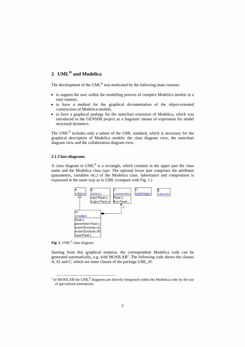
A class diagram in UMLH is a rectangle, which contains in the upper part the class name and the Modelica class type. The optional lower part comprises the attributes (parameters, variables etc.) of the Modelica class. Inheritance and composition is expressed in the same way as in UML (compare with Fig. 1.)

Fig. 1. UMLH class diagram

Starting from this graphical notation, the correspondent Modelica code can be generated automatically, e.g. with MOSILAB1. The following code shows the classes A, A1 and C, which are inner classes of the package UML_H:

1 In MOSILAB the UMLH diagrams are directly integrated within the Modelica code by the use

of specialized annotations.

2

package UML_H annotation(UMLH(ClassDiagram="<umlhclass><name>…); class A annotation(UMLH(classPos=[31,53])); end A; model A1 annotation(Icon(Text(extent=…,string="A1", …)); annotation(UMLH(classPos=[31,146])); extends A; event Boolean on; event Boolean off; Real x; input Real z; parameter Real y; C c; ...

end A1; connector C annotation(UMLH(classPos=[192,54])); Real u; flow Real i; end C; ... end UML_H;

2.2 Collaboration diagrams

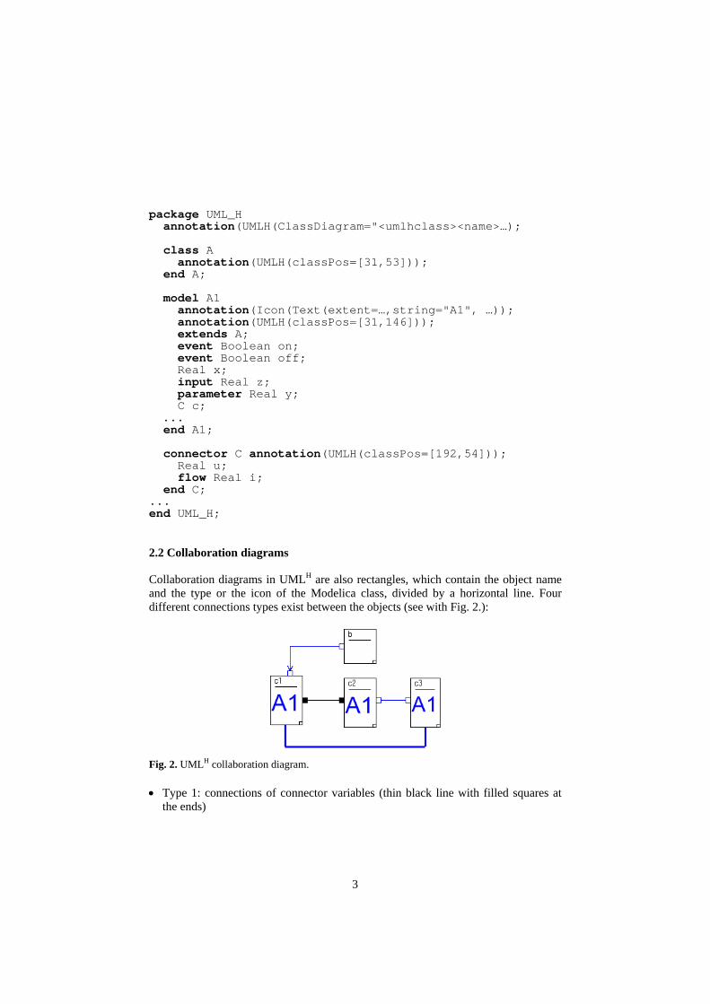
Collaboration diagrams in UMLH are also rectangles, which contain the object name and the type or the icon of the Modelica class, divided by a horizontal line. Four different connections types exist between the objects (see with Fig. 2.):

Fig. 2. UMLH collaboration diagram.

• Type 1: connections of connector variables (thin black line with filled squares at the ends)

3

• Type 2: connections of scalar variables (thin blue line with unfilled squares at the ends)

• Type 3: connections of scalar input/output variables (thin blue line with an arrow and a unfilled square)

• Type 4: multi-connections as a mixture of different connection types, e.g. type 1 and type 2 (fat blue line)

The following Modelica-code expresses the collaboration-diagram of Fig. 2: model System annotation(CompConnectors(CompConn(label="label2", points=[-81,52; -81,43; -24,43; -24,51]))); UML_H.A1 c1 annotation(extent=[-87,72; -74,52]); UML_H.A1 c2 annotation(extent=[-57,71; -44,51]); UML_H.A1 c3 annotation(extent=[-30,71; -18,51]); UML_H.B b annotation(extent=[-57,91; -44,77]); equation // connection type 1: connect(c1.c,c2.c)annotation(points=[-74,62;-57,62]); // connection type 2: c2.y=c3.y annotation(points=[-44,62; -30,62]); // connection type 4 (mixture of type 1 and 2): connect(c1.c,c3.c) annotation(label="label2"); c1.x=c3.x annotation(label="label2"); // connection type 3: b.y=c1.z annotation(points=[-57,84; -79,84; -79,72]); end System;

2.3 Statechart diagrams

A statechart diagram in UMLH is represented as a rectangle with round corners. In general, a statechart diagram contains several states and the transition definition between the states. Figure 3 shows four different types of States: • Initial states, symbolized with a black filled circle, • Final states, symbolized with a point in a unfilled circle, • Atomic states, with a flat internal structure, • Normal states, which can contain additional entry or exit actions and can be sub-

structured in further statechart diagrams.

4

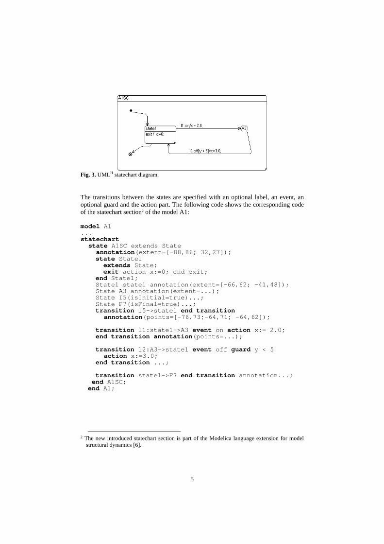
Fig. 3. UMLH statechart diagram.

The transitions between the states are specified with an optional label, an event, an optional guard and the action part. The following code shows the corresponding code of the statechart section2 of the model A1:

model A1 ... statechart state A1SC extends State annotation(extent=[-88,86; 32,27]); state State1 extends State; exit action x:=0; end exit; end State1; State1 state1 annotation(extent=[-66,62; -41,48]); State A3 annotation(extent=...); State I5(isInitial=true)...; State F7(isFinal=true)...; transition I5->state1 end transition

annotation(points=[-76,73;-64,71; -64,62]); transition l1:state1->A3 event on action x:= 2.0; end transition annotation(points=...); transition l2:A3->state1 event off guard y < 5

action x:=3.0; end transition ...; transition state1->F7 end transition annotation...; end A1SC; end A1;

2 The new introduced statechart section is part of the Modelica language extension for model

structural dynamics [6].

5

3 Example for UMLH-modeling

The modelling and simulation of a simplified Pool-Billiard game shall demonstrate the advantages of the graphical modelling with UMLH.

3.1 Model of a Pool-Billiard game

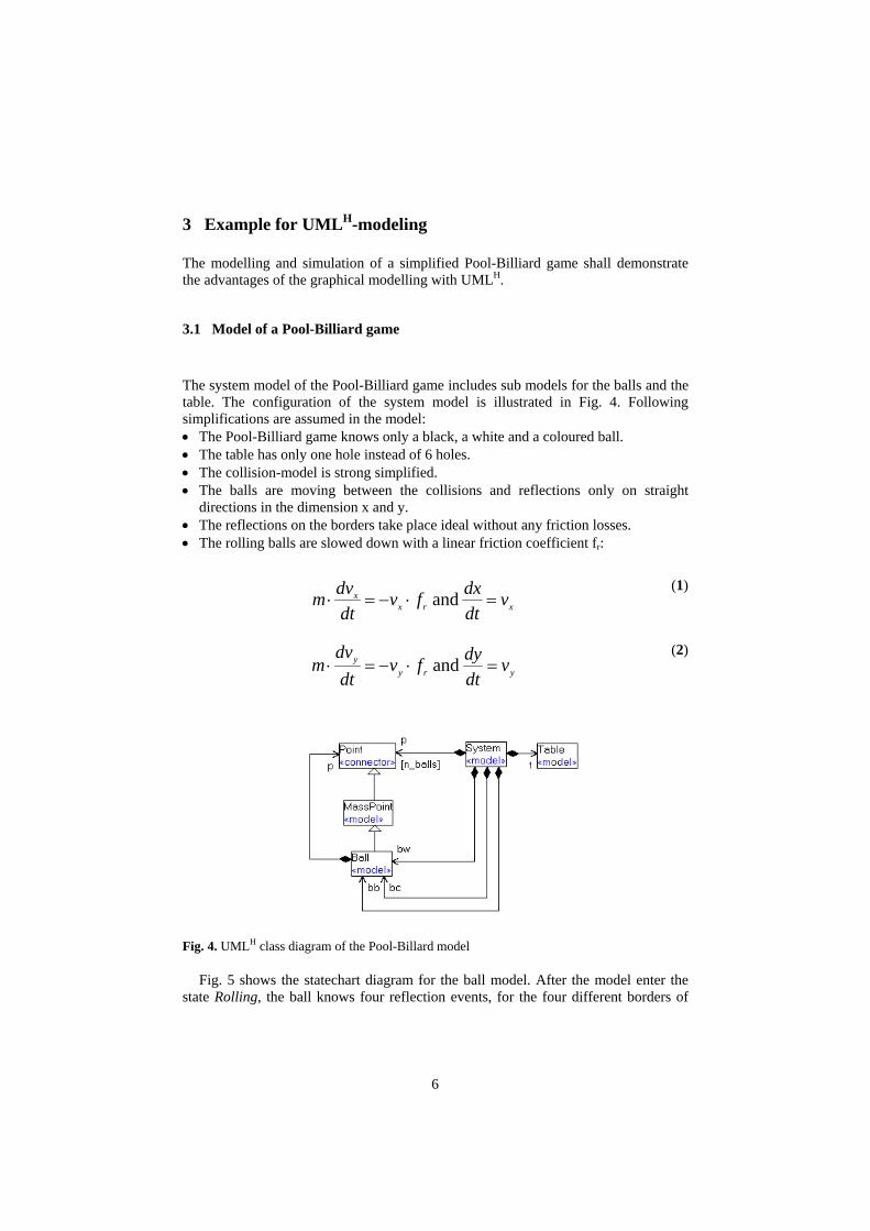
The system model of the Pool-Billiard game includes sub models for the balls and the table. The configuration of the system model is illustrated in Fig. 4. Following simplifications are assumed in the model: • The Pool-Billiard game knows only a black, a white and a coloured ball. • The table has only one hole instead of 6 holes. • The collision-model is strong simplified. • The balls are moving between the collisions and reflections only on straight

directions in the dimension x and y. • The reflections on the borders take place ideal without any friction losses. • The rolling balls are slowed down with a linear friction coefficient fr:

xrxx v

dtdxfv

dtdvm =⋅−=⋅ and

(1)

yryy v

dtdyfv

dtdv

m =⋅−=⋅ and (2)

Fig. 4. UMLH class diagram of the Pool-Billard model

Fig. 5 shows the statechart diagram for the ball model. After the model enter the state Rolling, the ball knows four reflection events, for the four different borders of

6

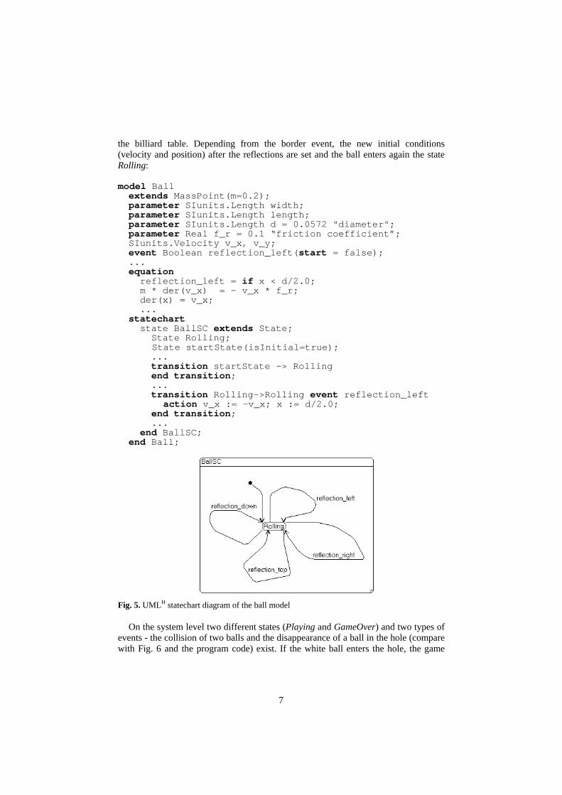
the billiard table. Depending from the border event, the new initial conditions (velocity and position) after the reflections are set and the ball enters again the state Rolling:

model Ball extends MassPoint(m=0.2); parameter SIunits.Length width; parameter SIunits.Length length; parameter SIunits.Length d = 0.0572 "diameter"; parameter Real f_r = 0.1 “friction coefficient”; SIunits.Velocity v_x, v_y; event Boolean reflection_left(start = false); ... equation reflection_left = if x < d/2.0; m * der(v_x) = - v_x * f_r; der(x) = v_x; ... statechart state BallSC extends State; State Rolling;

State startState(isInitial=true); ... transition startState -> Rolling end transition; ... transition Rolling->Rolling event reflection_left

action v_x := -v_x; x := d/2.0; end transition;

... end BallSC; end Ball;

Fig. 5. UMLH statechart diagram of the ball model

On the system level two different states (Playing and GameOver) and two types of events - the collision of two balls and the disappearance of a ball in the hole (compare with Fig. 6 and the program code) exist. If the white ball enters the hole, the game

7

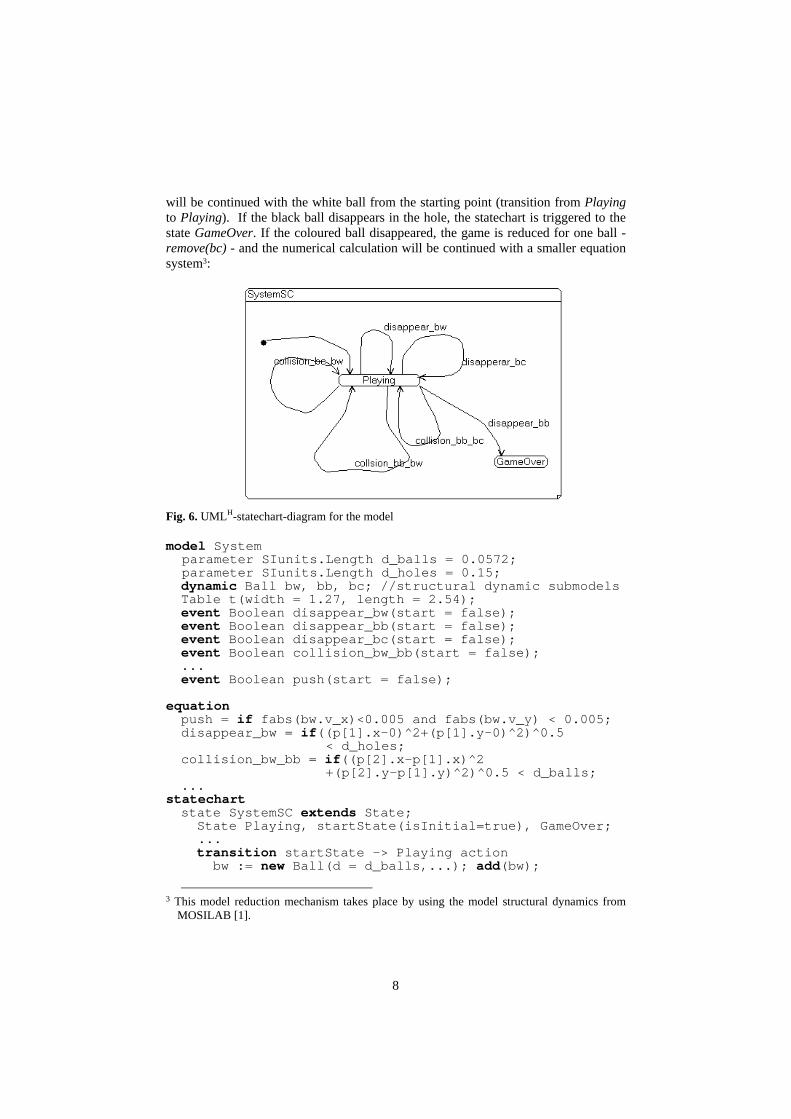
will be continued with the white ball from the starting point (transition from Playing to Playing). If the black ball disappears in the hole, the statechart is triggered to the state GameOver. If the coloured ball disappeared, the game is reduced for one ball - remove(bc) - and the numerical calculation will be continued with a smaller equation system3:

Fig. 6. UMLH-statechart-diagram for the model

model System parameter SIunits.Length d_balls = 0.0572; parameter SIunits.Length d_holes = 0.15; dynamic Ball bw, bb, bc; //structural dynamic submodels Table t(width = 1.27, length = 2.54); event Boolean disappear_bw(start = false); event Boolean disappear_bb(start = false); event Boolean disappear_bc(start = false); event Boolean collision_bw_bb(start = false); ... event Boolean push(start = false);

equation push = if fabs(bw.v_x)<0.005 and fabs(bw.v_y) < 0.005; disappear_bw = if((p[1].x-0)^2+(p[1].y-0)^2)^0.5

< d_holes; collision_bw_bb = if((p[2].x-p[1].x)^2

+(p[2].y-p[1].y)^2)^0.5 < d_balls; ...

statechart state SystemSC extends State; State Playing, startState(isInitial=true), GameOver;

... transition startState -> Playing action bw := new Ball(d = d_balls,...); add(bw);

3 This model reduction mechanism takes place by using the model structural dynamics from

MOSILAB [1].

8

bb := new Ball(...); add(bb); bc := new Ball(...); add(bc); end transition;

transition Playing->Playing event disappear_bw action ... remove(bw); bw := new Ball(x(start=1.27/2.9), y(start=0.6)); end transition;

transition Playing->Playing event disappear_bc action ... remove(bb); end transition;

transition Playing -> GameOver event disappear_bb end transition;

transition Playing->Playing event collision_bw_bb action v_x := bw.v_x; v_y := bw.v_y; bw.v_x := bb.v_x; bw.v_y := bb.v_y; bb.v_x := v_x; bb.v_y := v_y; end transition; end SystemSC;

end System;

3.1 Simulation experiment

The following simulation experiment illustrates the previous explained behaviour of the Pool-Billiard game. The parameter of the model are set in a manner, that all different types of events (1: collision of two balls, 2: reflection on a border, 3: disappearing in the hole) are present during the simulation experiment (see Fig. 7).

11

22

33

Fig. 7. Event types in the Pool-Billiard game Figure 8 show the positions and the Figures 9 and 10 the reflection and collision

events of the white and the black ball during a simulation period of 4 seconds.

9

Fig. 8. x- and y-positions of the white and the black ball

Fig. 9. Collision events of the white and the black ball

10

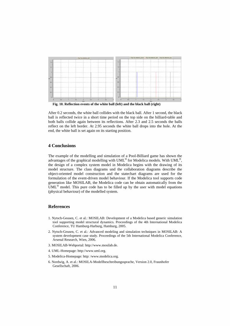
Fig. 10. Reflection events of the white ball (left) and the black ball (right)

After 0.2 seconds, the white ball collides with the black ball. After 1 second, the black ball is reflected twice in a short time period on the top side on the billiard-table and both balls collide again between its reflections. After 2.3 and 2.5 seconds the balls reflect on the left border. At 2.95 seconds the white ball drops into the hole. At the end, the white ball is set again on its starting position.

4 Conclusions

The example of the modelling and simulation of a Pool-Billiard game has shown the advantages of the graphical modelling with UMLH for Modelica models. With UMLH, the design of a complex system model in Modelica begins with the drawing of its model structure. The class diagrams und the collaboration diagrams describe the object-oriented model construction and the statechart diagrams are used for the formulation of the event-driven model behaviour. If the Modelica tool supports code generation like MOSILAB, the Modelica code can be obtain automatically from the UMLH model. This pure code has to be filled up by the user with model equations (physical behaviour) of the modelled system.

References

1. Nytsch-Geusen, C. et al.: MOSILAB: Development of a Modelica based generic simulation tool supporting model structural dynamics. Proceedings of the 4th International Modelica Conference, TU Hamburg-Harburg, Hamburg, 2005.

2. Nytsch-Geusen, C. et al.: Advanced modeling and simulation techniques in MOSILAB: A system development case study. Proceedings of the 5th International Modelica Conference, Arsenal Research, Wien, 2006.

3. MOSILAB-Webportal: http://www.mosilab.de. 4. UML-Homepage: http://www.uml.org. 5. Modelica-Homepage: http: /www.modelica.org. 6. Nordwig, A. et al.: MOSILA-Modellbeschreibungssprache, Version 2.0, Fraunhofer

Gesellschaft, 2006.

11

Towards Unified System Modeling with the ModelicaML UML Profile

Adrian Pop, David Akhvlediani, Peter Fritzson

Programming Environments Lab, Department of Computer and Information Science

Linköping University, SE-581 83 Linköping, Sweden adrpo, petfr@ida.liu.se

Abstract. In order to support the development of complex products, modeling tools and processes need to support co-design of software and hardware in an integrated way. Modelica is the major object-oriented mathematical modeling language for component-oriented modeling of complex physical systems and UML is the dominant graphical modeling notation for software. In this paper we propose ModelicaML UML profile as an integration of Modelica and UML. The profile combines the major UML diagrams with Modelica graphic connec-tion diagrams and is based on the System Modeling Language (SysML) profile.

1 Introduction

The development in system modeling has come to the point where complete modeling of systems is possible, e.g. the complete propulsion system, fuel system, hydraulic actuation system, etc., including embedded software can be modeled and simulated concurrently. This does not mean that all components are dealt with down to the very smallest details of their behavior. It does, however, mean that all functionality is mod-eled, at least qualitatively.

In this paper, a UML profile for Modelica, named ModelicaML, is proposed. The ModelicaML UML profile is based on the OMG SysML™ (Systems Modeling Lan-guage) profile and reuses its artifacts required for system specification. SysML dia-grams are also extended to support all Modelica constructs. We argue that with Mode-licaML system engineers are able to specify entire systems, starting from require-ments, continuing with behavior and finally perform system simulations.

2 SysML and Modelica

The Unified Modeling Language (UML) has been created to assist software develop-ment processes by providing means to capture software system structure and behav-ior. This evolved into the main standard for Model Driven Development [5].

The System Modeling Language (SysML) [4] is a graphical modeling language for systems engineering applications. SysML was developed by systems engineering ex-

13

perts, and was adopted by OMG in 2006. SysML is built on top of UML and tailored to the needs of system engineers by supporting specification, analysis, design, verifi-cation and validation of broad range of systems and system-of-systems.

The main goal behind SysML is to unify and replace different document-centric approaches in the system engineering field with a single systems modeling language. A single model-centric approach improves communication, assists to manage com-plex system design and allows its early validation and verification.

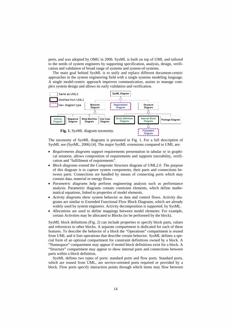
The taxonomy of SysML diagrams is presented in Fig. 1. For a full description of SysML see (SysML, 2006) [4]. The major SysML extensions compared to UML are:

• Requirements diagrams support requirements presentation in tabular or in graphi-cal notation, allows composition of requirements and supports traceability, verifi-cation and “fulfillment of requirements”.

• Block diagrams extend the Composite Structure diagram of UML2.0. The purpose of this diagram is to capture system components, their parts and connections be-tween parts. Connections are handled by means of connecting ports which may contain data, material or energy flows.

• Parametric diagrams help perform engineering analysis such as performance analysis. Parametric diagrams contain constraint elements, which define mathe-matical equations, linked to properties of model elements.

• Activity diagrams show system behavior as data and control flows. Activity dia-grams are similar to Extended Functional Flow Block Diagrams, which are already widely used by system engineers. Activity decomposition is supported. by SysML.

• Allocations are used to define mappings between model elements: For example, certain Activities may be allocated to Blocks (to be performed by the block).

SysML block definitions (Fig. 2) can include properties to specify block parts, values and references to other blocks. A separate compartment is dedicated for each of these features. To describe the behavior of a block the “Operations” compartment is reused from UML and it lists operations that describe certain behavior. SysML defines a spe-cial form of an optional compartment for constraint definitions owned by a block. A “Namespace” compartment may appear if nested block definitions exist for a block. A “Structure” compartment may appear to show internal parts and connections between parts within a block definition.

SysML defines two types of ports: standard ports and flow ports. Standard ports, which are reused from UML, are service-oriented ports required or provided by a block. Flow ports specify interaction points through which items may flow between

Fig. 1. SysML diagram taxonomy.

14

blocks, and between blocks and environment. A flow port definition may include sin-gle item specification or complex flow specification through the FlowSpecification interface; flow ports define what “can” flow between the block and its environment. Flow direction can be specified for a flow port in SysML. SysML also defines a no-tion of Item flows that specify “what” does flow in a particular usage context.

Fig. 2. SysML block definitions.

2.1 Modelica

Modelica [2] [3] is a modern language for equation-based object-oriented mathemati-cal modeling primarily of physical systems. Several tools, ranging from open-source as OpenModelica [1], to commercial like Dymola [11] or MathModelica [10] support the Modelica specification.

The language allows defining models in a declarative manner, modularly and hier-archically and combining various formalisms expressible in the more general Mode-lica formalism. The multidomain capability of Modelica allows combining electrical, mechanical, hydraulic, thermodynamic, etc., model components within the same ap-plication model. In short, Modelica has improvements in several important areas:

• Object-oriented mathematical modeling. This technique makes it possible to create model components, which are employed to support hierarchical structuring, reuse, and evolution of large and complex models covering multiple technology domains.

• Physical modeling of multiple application domains. Model components can corre-spond to physical objects in the real world, in contrast to established techniques that require conversion to “signal” blocks with fixed input/output causality. In Modelica the structure of the model naturally correspond to the structure of the physical system in contrast to block-oriented modeling tools.

• Acausal modeling. Modeling is based on equations instead of assignment state-ments as in traditional input/output block abstractions. Direct use of equations sig-nificantly increases re-usability of model components, since components adapt to the data flow context in which they are used.

15

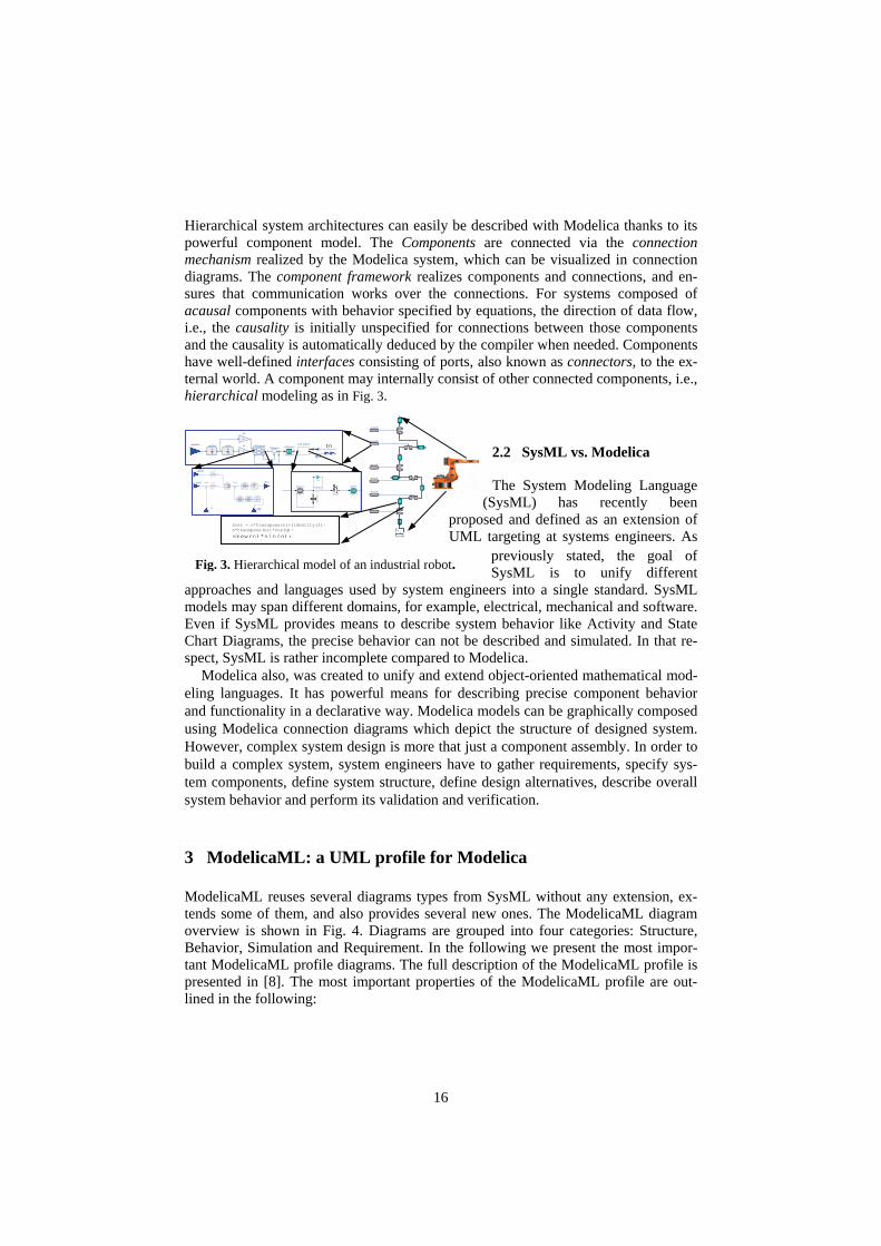
Fig. 3. Hierarchical model of an industrial robot.

inertialx

y

axis1

axis2

axis3

axis4

axis5

axis6

r3Drive1

1r3Motor

r3ControlqdRef1

S

qRef1

S

k2

i

k1

i

qddRef cut joint

l

qd

tn

rate2

b(s)

a(s)

rate3

340.8

S

rate1

b(s)

a(s)

tacho1

PT1

Kd

0.03

w Sum

-

sum

+1

+1

pSum

-

Kv

0.3

tacho2

b(s)

a(s)

q qd

iRefqRef

qdRef

Jmotor=J

gear=i

spring=c

fric

=Rv0

Srel

joint=0

S

Srel = n*transpose(n)+(identity(3)- n*transpose(n))*cos(q)-

skew(n)*sin(q);

Hierarchical system architectures can easily be described with Modelica thanks to its powerful component model. The Components are connected via the connection mechanism realized by the Modelica system, which can be visualized in connection diagrams. The component framework realizes components and connections, and en-sures that communication works over the connections. For systems composed of acausal components with behavior specified by equations, the direction of data flow, i.e., the causality is initially unspecified for connections between those components and the causality is automatically deduced by the compiler when needed. Components have well-defined interfaces consisting of ports, also known as connectors, to the ex-ternal world. A component may internally consist of other connected components, i.e., hierarchical modeling as in Fig. 3.

2.2 SysML vs. Modelica

The System Modeling Language (SysML) has recently been

proposed and defined as an extension of UML targeting at systems engineers. As

previously stated, the goal of SysML is to unify different

approaches and languages used by system engineers into a single standard. SysML models may span different domains, for example, electrical, mechanical and software. Even if SysML provides means to describe system behavior like Activity and State Chart Diagrams, the precise behavior can not be described and simulated. In that re-spect, SysML is rather incomplete compared to Modelica.

Modelica also, was created to unify and extend object-oriented mathematical mod-eling languages. It has powerful means for describing precise component behavior and functionality in a declarative way. Modelica models can be graphically composed using Modelica connection diagrams which depict the structure of designed system. However, complex system design is more that just a component assembly. In order to build a complex system, system engineers have to gather requirements, specify sys-tem components, define system structure, define design alternatives, describe overall system behavior and perform its validation and verification.

3 ModelicaML: a UML profile for Modelica

ModelicaML reuses several diagrams types from SysML without any extension, ex-tends some of them, and also provides several new ones. The ModelicaML diagram overview is shown in Fig. 4. Diagrams are grouped into four categories: Structure, Behavior, Simulation and Requirement. In the following we present the most impor-tant ModelicaML profile diagrams. The full description of the ModelicaML profile is presented in [8]. The most important properties of the ModelicaML profile are out-lined in the following:

16

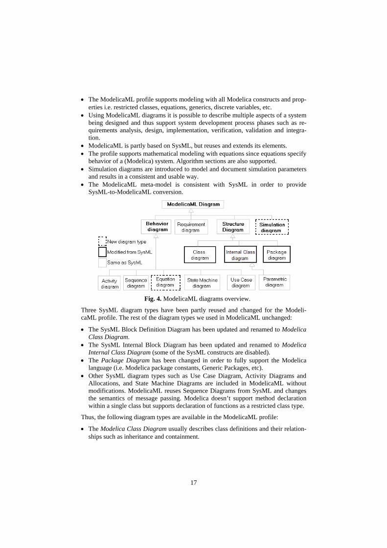
• The ModelicaML profile supports modeling with all Modelica constructs and prop-erties i.e. restricted classes, equations, generics, discrete variables, etc.

• Using ModelicaML diagrams it is possible to describe multiple aspects of a system being designed and thus support system development process phases such as re-quirements analysis, design, implementation, verification, validation and integra-tion.

• ModelicaML is partly based on SysML, but reuses and extends its elements. • The profile supports mathematical modeling with equations since equations specify

behavior of a (Modelica) system. Algorithm sections are also supported. • Simulation diagrams are introduced to model and document simulation parameters

and results in a consistent and usable way. • The ModelicaML meta-model is consistent with SysML in order to provide

SysML-to-ModelicaML conversion.

Fig. 4. ModelicaML diagrams overview.

Three SysML diagram types have been partly reused and changed for the Modeli-caML profile. The rest of the diagram types we used in ModelicaML unchanged:

• The SysML Block Definition Diagram has been updated and renamed to Modelica Class Diagram.

• The SysML Internal Block Diagram has been updated and renamed to Modelica Internal Class Diagram (some of the SysML constructs are disabled).

• The Package Diagram has been changed in order to fully support the Modelica language (i.e. Modelica package constants, Generic Packages, etc).

• Other SysML diagram types such as Use Case Diagram, Activity Diagrams and Allocations, and State Machine Diagrams are included in ModelicaML without modifications. ModelicaML reuses Sequence Diagrams from SysML and changes the semantics of message passing. Modelica doesn’t support method declaration within a single class but supports declaration of functions as a restricted class type.

Thus, the following diagram types are available in the ModelicaML profile:

• The Modelica Class Diagram usually describes class definitions and their relation-ships such as inheritance and containment.

17

• The Modelica Internal Class Diagram describes the internal class structure and interconnections between parts.

• The Package Diagram groups logically connected user defined elements into pack-ages. In ModelicaML the primarily purpose of this diagram is to support the specif-ics of the Modelica packages.

• Activity, Sequence, State Machine, Use Case, Parametric and Requirements dia-grams have been reused without modification from SysML.

• Two new diagrams, Simulation Diagram and Equation Diagram, not present in SysML, have been included in the ModelicaML profile.

3.1 Package Diagram

A UML Package is a general purpose model element for grouping other elements within a separate namespace. With a help of packages, designers are able group ele-ments to correspond to different structures/views of a system. ModelicaML extends UML packages in order to support Modelica packaging features, in particular: pack-age inheritance, generic packages, constant declaration within a package, package “instantiation” and renaming import (see [2] for Modelica packages details).

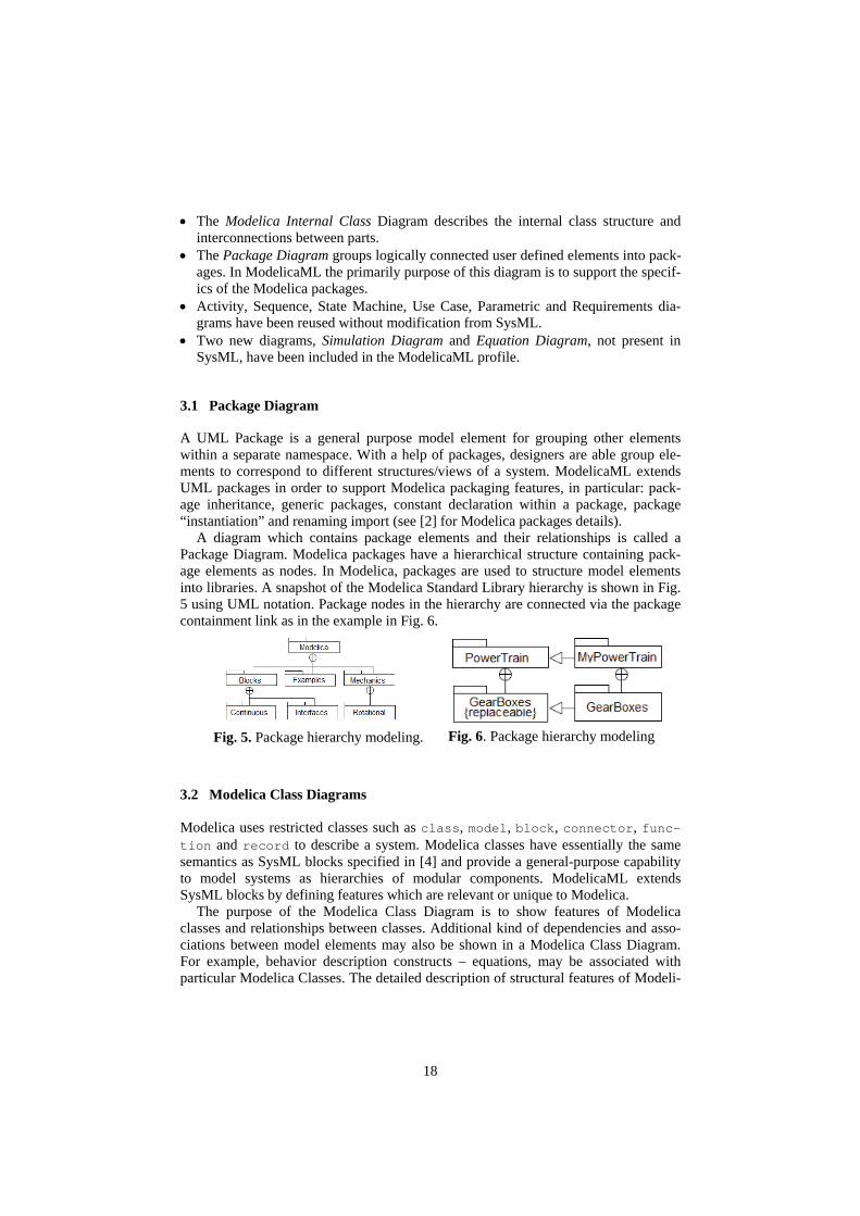
A diagram which contains package elements and their relationships is called a Package Diagram. Modelica packages have a hierarchical structure containing pack-age elements as nodes. In Modelica, packages are used to structure model elements into libraries. A snapshot of the Modelica Standard Library hierarchy is shown in Fig. 5 using UML notation. Package nodes in the hierarchy are connected via the package containment link as in the example in Fig. 6.

Fig. 5. Package hierarchy modeling.

Fig. 6. Package hierarchy modeling

3.2 Modelica Class Diagrams

Modelica uses restricted classes such as class, model, block, connector, func-tion and record to describe a system. Modelica classes have essentially the same semantics as SysML blocks specified in [4] and provide a general-purpose capability to model systems as hierarchies of modular components. ModelicaML extends SysML blocks by defining features which are relevant or unique to Modelica.

The purpose of the Modelica Class Diagram is to show features of Modelica classes and relationships between classes. Additional kind of dependencies and asso-ciations between model elements may also be shown in a Modelica Class Diagram. For example, behavior description constructs – equations, may be associated with particular Modelica Classes. The detailed description of structural features of Modeli-

18

caML is provided below. ModelicaML structural extensions are defined based on the SysML block definition outlined in section 2.

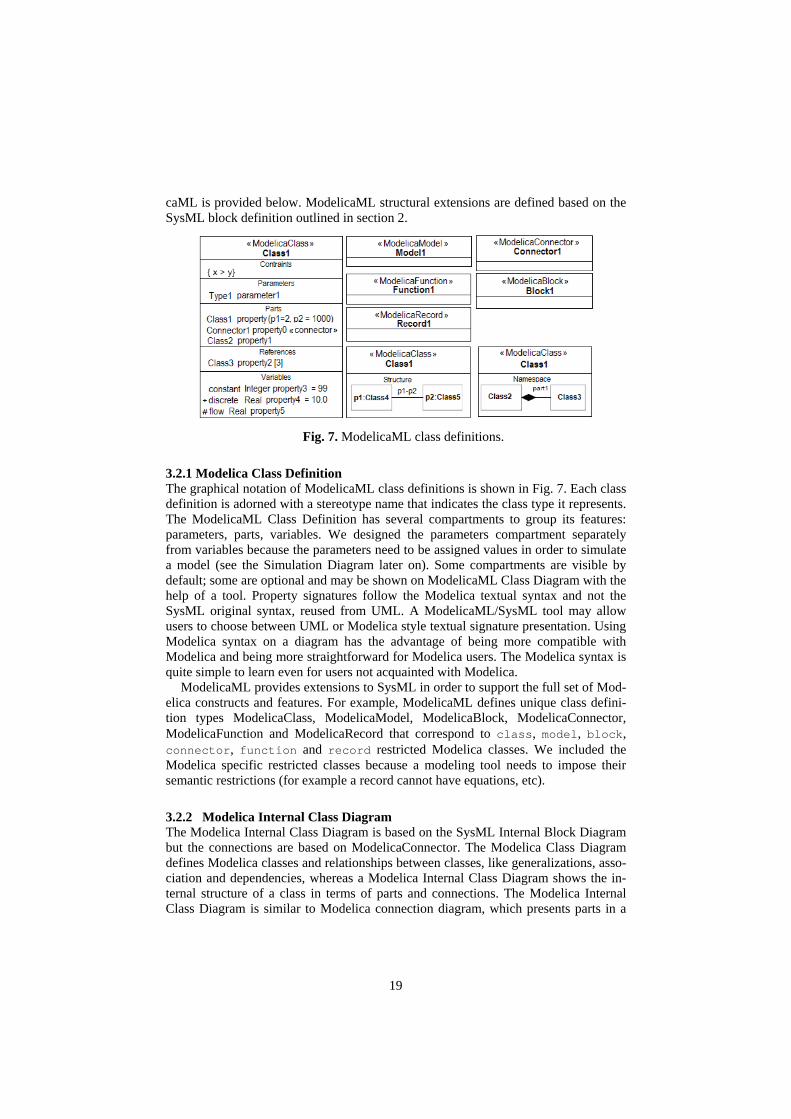
Fig. 7. ModelicaML class definitions.

3.2.1 Modelica Class Definition The graphical notation of ModelicaML class definitions is shown in Fig. 7. Each class definition is adorned with a stereotype name that indicates the class type it represents. The ModelicaML Class Definition has several compartments to group its features: parameters, parts, variables. We designed the parameters compartment separately from variables because the parameters need to be assigned values in order to simulate a model (see the Simulation Diagram later on). Some compartments are visible by default; some are optional and may be shown on ModelicaML Class Diagram with the help of a tool. Property signatures follow the Modelica textual syntax and not the SysML original syntax, reused from UML. A ModelicaML/SysML tool may allow users to choose between UML or Modelica style textual signature presentation. Using Modelica syntax on a diagram has the advantage of being more compatible with Modelica and being more straightforward for Modelica users. The Modelica syntax is quite simple to learn even for users not acquainted with Modelica.

ModelicaML provides extensions to SysML in order to support the full set of Mod-elica constructs and features. For example, ModelicaML defines unique class defini-tion types ModelicaClass, ModelicaModel, ModelicaBlock, ModelicaConnector, ModelicaFunction and ModelicaRecord that correspond to class, model, block, connector, function and record restricted Modelica classes. We included the Modelica specific restricted classes because a modeling tool needs to impose their semantic restrictions (for example a record cannot have equations, etc).

3.2.2 Modelica Internal Class Diagram The Modelica Internal Class Diagram is based on the SysML Internal Block Diagram but the connections are based on ModelicaConnector. The Modelica Class Diagram defines Modelica classes and relationships between classes, like generalizations, asso-ciation and dependencies, whereas a Modelica Internal Class Diagram shows the in-ternal structure of a class in terms of parts and connections. The Modelica Internal Class Diagram is similar to Modelica connection diagram, which presents parts in a

19

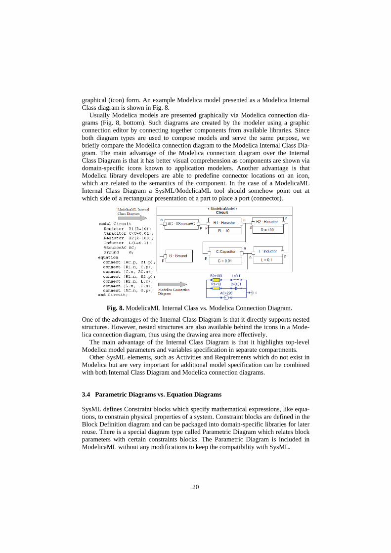
graphical (icon) form. An example Modelica model presented as a Modelica Internal Class diagram is shown in Fig. 8.

Usually Modelica models are presented graphically via Modelica connection dia-grams (Fig. 8, bottom). Such diagrams are created by the modeler using a graphic connection editor by connecting together components from available libraries. Since both diagram types are used to compose models and serve the same purpose, we briefly compare the Modelica connection diagram to the Modelica Internal Class Dia-gram. The main advantage of the Modelica connection diagram over the Internal Class Diagram is that it has better visual comprehension as components are shown via domain-specific icons known to application modelers. Another advantage is that Modelica library developers are able to predefine connector locations on an icon, which are related to the semantics of the component. In the case of a ModelicaML Internal Class Diagram a SysML/ModelicaML tool should somehow point out at which side of a rectangular presentation of a part to place a port (connector).

Fig. 8. ModelicaML Internal Class vs. Modelica Connection Diagram.

One of the advantages of the Internal Class Diagram is that it directly supports nested structures. However, nested structures are also available behind the icons in a Mode-lica connection diagram, thus using the drawing area more effectively.

The main advantage of the Internal Class Diagram is that it highlights top-level Modelica model parameters and variables specification in separate compartments.

Other SysML elements, such as Activities and Requirements which do not exist in Modelica but are very important for additional model specification can be combined with both Internal Class Diagram and Modelica connection diagrams.

3.4 Parametric Diagrams vs. Equation Diagrams

SysML defines Constraint blocks which specify mathematical expressions, like equa-tions, to constrain physical properties of a system. Constraint blocks are defined in the Block Definition diagram and can be packaged into domain-specific libraries for later reuse. There is a special diagram type called Parametric Diagram which relates block parameters with certain constraints blocks. The Parametric Diagram is included in ModelicaML without any modifications to keep the compatibility with SysML.

20

The Modelica class behavior is usually described by equations, which also constrain Modelica class parameters, and have a domain-specific usage. SysML constraint blocks are less powerful means of domain model description than Modelica equations. Modelica equations include some type of equations, which cannot be modeled using Constraint blocks, i.e.: if, for, when equations. Also, modeling complexity is an issue, as for example in Fig. 9 there are only four equations, and the diagram is al-ready quite complex. However, grouping constraint blocks into libraries can be useful for system engineers who use Modelica and SysML. SysML Parametric diagram may be used during the initial design phase, when equations related to a class are being identified using Parametric Diagrams and finally associated (via an Equation Dia-gram) with a Modelica class or set of classes.

Fig. 9. Parametric Diagram Example

partial class TwoPin Pin p, n; Voltage v; Current i; equation v = p.v – n.v; 0 = p.i + n.i; i = p.i; end TwoPin; class Resistor extends TwoPin; parameter Real R(unit = "Ohm"); equation R * I = v; end Resistor;

Fig. 10. Equation modeling example with a Modelica Class Diagram.

In Fig. 10, Fig. 11 we present examples of behavior specification via Equation Dia-grams in ModelicaML. Equations do not prescribe a certain data flow direction which means that the order in which equations appear in a model do not influence their meaning and semantics. The only requirement for a system of equations is to be solv-able. For further details about Modelica equations, see [2]. Besides simple equality equations, Modelica allows other kind of equations be presented within a model. For each of such kind of equations (i.e. when/if/initial equations) ModelicaML defines a graphical construct. It’s up to designer to decide whether to use simple equations block representation or specific construct for equation modeling. Algorithm sections are modeled similar to equations, as text.

21

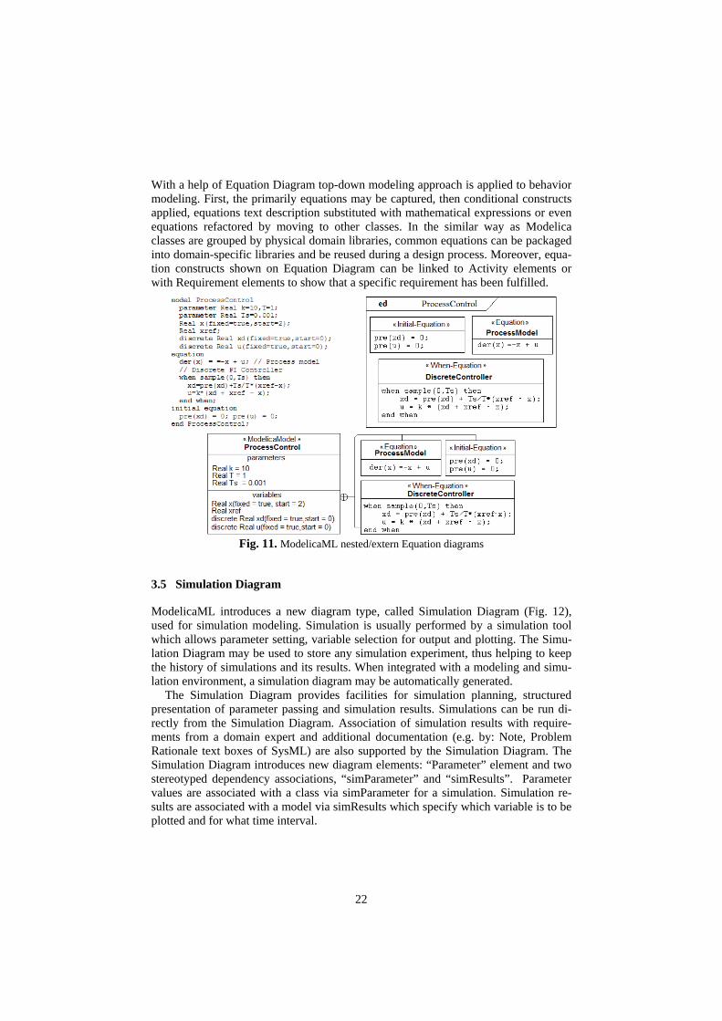
With a help of Equation Diagram top-down modeling approach is applied to behavior modeling. First, the primarily equations may be captured, then conditional constructs applied, equations text description substituted with mathematical expressions or even equations refactored by moving to other classes. In the similar way as Modelica classes are grouped by physical domain libraries, common equations can be packaged into domain-specific libraries and be reused during a design process. Moreover, equa-tion constructs shown on Equation Diagram can be linked to Activity elements or with Requirement elements to show that a specific requirement has been fulfilled.

Fig. 11. ModelicaML nested/extern Equation diagrams

3.5 Simulation Diagram

ModelicaML introduces a new diagram type, called Simulation Diagram (Fig. 12), used for simulation modeling. Simulation is usually performed by a simulation tool which allows parameter setting, variable selection for output and plotting. The Simu-lation Diagram may be used to store any simulation experiment, thus helping to keep the history of simulations and its results. When integrated with a modeling and simu-lation environment, a simulation diagram may be automatically generated.

The Simulation Diagram provides facilities for simulation planning, structured presentation of parameter passing and simulation results. Simulations can be run di-rectly from the Simulation Diagram. Association of simulation results with require-ments from a domain expert and additional documentation (e.g. by: Note, Problem Rationale text boxes of SysML) are also supported by the Simulation Diagram. The Simulation Diagram introduces new diagram elements: “Parameter” element and two stereotyped dependency associations, “simParameter” and “simResults”. Parameter values are associated with a class via simParameter for a simulation. Simulation re-sults are associated with a model via simResults which specify which variable is to be plotted and for what time interval.

22

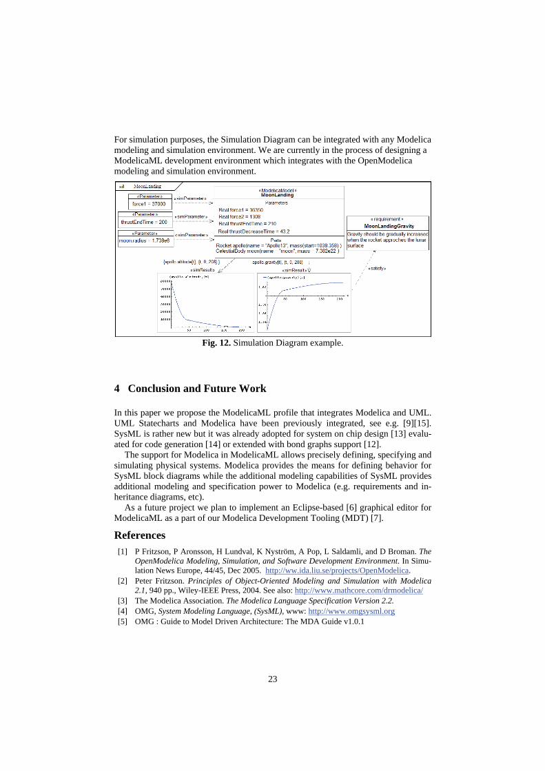
For simulation purposes, the Simulation Diagram can be integrated with any Modelica modeling and simulation environment. We are currently in the process of designing a ModelicaML development environment which integrates with the OpenModelica modeling and simulation environment.

Fig. 12. Simulation Diagram example.

4 Conclusion and Future Work

In this paper we propose the ModelicaML profile that integrates Modelica and UML. UML Statecharts and Modelica have been previously integrated, see e.g. [9][15]. SysML is rather new but it was already adopted for system on chip design [13] evalu-ated for code generation [14] or extended with bond graphs support [12].

The support for Modelica in ModelicaML allows precisely defining, specifying and simulating physical systems. Modelica provides the means for defining behavior for SysML block diagrams while the additional modeling capabilities of SysML provides additional modeling and specification power to Modelica (e.g. requirements and in-heritance diagrams, etc).

As a future project we plan to implement an Eclipse-based [6] graphical editor for ModelicaML as a part of our Modelica Development Tooling (MDT) [7].

References [1] P Fritzson, P Aronsson, H Lundval, K Nyström, A Pop, L Saldamli, and D Broman. The

OpenModelica Modeling, Simulation, and Software Development Environment. In Simu-lation News Europe, 44/45, Dec 2005. http://ww.ida.liu.se/projects/OpenModelica.

[2] Peter Fritzson. Principles of Object-Oriented Modeling and Simulation with Modelica 2.1, 940 pp., Wiley-IEEE Press, 2004. See also: http://www.mathcore.com/drmodelica/

[3] The Modelica Association. The Modelica Language Specification Version 2.2. [4] OMG, System Modeling Language, (SysML), www: http://www.omgsysml.org [5] OMG : Guide to Model Driven Architecture: The MDA Guide v1.0.1

23

[6] Eclipse.Org, www: http://www.eclipse.org/ [7] A Pop, P Fritzson, A Remar, E Jagudin, and D Akhvlediani. OpenModelica Development

Environment with Eclipse Integration for Browsing, Modeling, and Debugging. In Proc of the Modelica'2006, Vienna, Austria, Sept. 4-5, 2006.

[8] David Akhvlediani. Design and implementation of a UML profile for Modelica/SysML. Final Thesis, LITH-IDA-EX--06/061—SE, April 2007.

[9] J.Ferreira, J. Estima, Modeling hybrid systems using Statechars and Modelica”. 7th IEEE Intl. Conf. on Emerging Technologies and Factory Automation, October 1999, Spain.

[10] MathCore Engineering AB, MathModelica http://www.mathcore.com [11] Dynasim AB, Dymola, http://www.dynasim.com [12] Skander Turki, Thierry Soriano, A SysML Extension for Bond Graphs Support, Proc. of

the International Conference on Technology and Automation (ICTA), Greece, 2005 [13] Yves Vanderperren, Wim Dehane, SysML and Systems Engineering Applied to UML-

Based SoC Design, Proc. of the 2nd UML-SoC Workshop at 42nd DAC, USA, 2005. [14] Yves Vanderperren, Wim Dehane, From UML/SysML to Matlab/Simulink, Proceedings

of the Conference on Design, Automation and Test in Europe (DATE), Munich, 2006. [15] André Nordwig. Formal Integration of Structural Dynamics into the Object-Oriented

Modeling of Hybrid Systems. ESM 2002: 128-134.

24

Developing Dependable Automotive Embedded Systems using the EAST-ADL; representing continuous time

systems in SysML

Carl-Johan Sjöstedt1, De-Jiu Chen1, Phillipe Cuenot2, Patrick Frey3, Rolf Johansson4, Henrik Lönn5, David Servat6, Martin Törngren1

1 Royal Institute of Technology, SE-100 44 Stockholm, Sweden

2 Siemens VDO, 1 Avenue Paul Ourliac, BP 1149 31036 Toulouse Cedex 1, France 3 ETAS GmbH, Borsigstr. 14, 70469 Stuttgart, Germany

4 Mentor Graphics, Theres Svenssons Gata 15, SE-417 55 Gothenburg, Sweden 5 Volvo Technology Corporation, Electronics and Software, SE-405 08 Gothenburg, Sweden

6 CEA List, Comtmissariat à l'Énergie Atomique Saclay, F-91191 Gif sur Yvette Cedex, France

1 carlj, chen, martin@md.kth.se 2 philippe.cuenot@siemens.com

3 patrick.frey@etas.de 4 rolf_johansson@mentor.com

5 henrik.lonn@volvo.com 6 david.servat@cea.fr

Abstract. The architectural description language for automotive embedded systems EAST-ADL is presented in this paper. The aim of the EAST-ADL language is to provide a comprehensive systems modeling approach as a means to keep the engineering information within one structure. This facilitates systems integration and enables consistent systems analysis. The EAST-ADL encompasses structural information at different abstraction levels, requirements and variability modeling. The EAST-ADL is implemented as a UML2 profile and is harmonized with AUTOSAR and a subset of SysML. Currently, different ways to model behavior natively in the language are investigated. An approach for using SysML parametric diagrams to describe equations in composed physical systems is proposed. An example system is modeled and discussed. It is highlighted that parametric diagrams lacks support for separation between effort and flow variables, and why this separation would be desired in order to model composed physical systems. An alternative approach by use of SysML activity diagrams is also discussed. Keywords: EAST-ADL, automotive embedded systems, UML, SysML, parametric diagrams, physical modeling, continuous systems, Modelica

1 Introduction and goals

New functionality in automotive systems is increasingly realized by software and electronics. A system level function, such as an adaptive cruise controller will then be

25

partitioned into functions that are realized by software and electronics (the vehicle embedded system), and other functions realized in mechanical subsystems. The complexity of embedded systems calls for a more rigorous approach to system development compared to current state of practice. A critical issue is the management of the engineering information that defines the embedded system. This issue should be understood in the light of current development practice which is characterized by the involvement of a very large number of specialists/groups/companies: all participants are working on the same system but using different tools, models, information formats, and subsets of the complete information. In current practices, integration of artifacts from different parties takes place at a very late stage of the development process where electronic control units are integrated into the overall embedded system of a vehicle. There is a need to shift this hardware level integration to model level integration [2]. Model based development has the potential to improve the cost efficiency of the products including their quality.

In this paper, we will discuss one aspect of model based development, the modeling of the environment to the developed system. Environment models serve several purposes in an architecture description language (ADL). An environment model defines implicitly the context and relevant use of the systems and functions in the embedded systems architecture. Validation activities such as simulation, interface consistency, formal verification all benefit from an environment model. The environment of an automotive embedded system may include all kinds of systems and behaviors that are part of the embedded system itself. The focus here is on physical continuous time systems. In particular we investigate the representation of continuous systems in SysML parametric diagrams, using Modelica [6] compatible constructs.

The presented approach is a part of an effort to refine an architecture description language for automotive embedded systems. An initial version of this language, EAST-ADL, was developed in the EAST-EEA project [19]. Further work on the the language is pursued in the ATESST project [17]. For other aspects of the EAST-ADL, see [3].

2 Overview of the EAST-ADL

The EAST-ADL is intended to support the development of automotive embedded software by capturing all the related engineering information. The scope is the embedded system (hardware and software) of a vehicle and its environment. The EAST-ADL system model is organized in parts representing different levels of abstraction and thus reflects different views and details of the architecture. The levels implicitly reflect different stages of an engineering process, but the detailed process definition is company specific.

The EAST-ADL language constructs support: • vehicle feature modeling including concepts to support product families • concepts for defining variability in all parts of a model • vehicle environment modeling to define context and perform validation

26

• structural and behavioral modeling of software and hardware entities in the context of distributed systems.

• requirements modeling and tracing with all modeling entities • other information part of the system description, such as a definition of component

timing and failure modes, necessary for design space exploration and system verification purposes

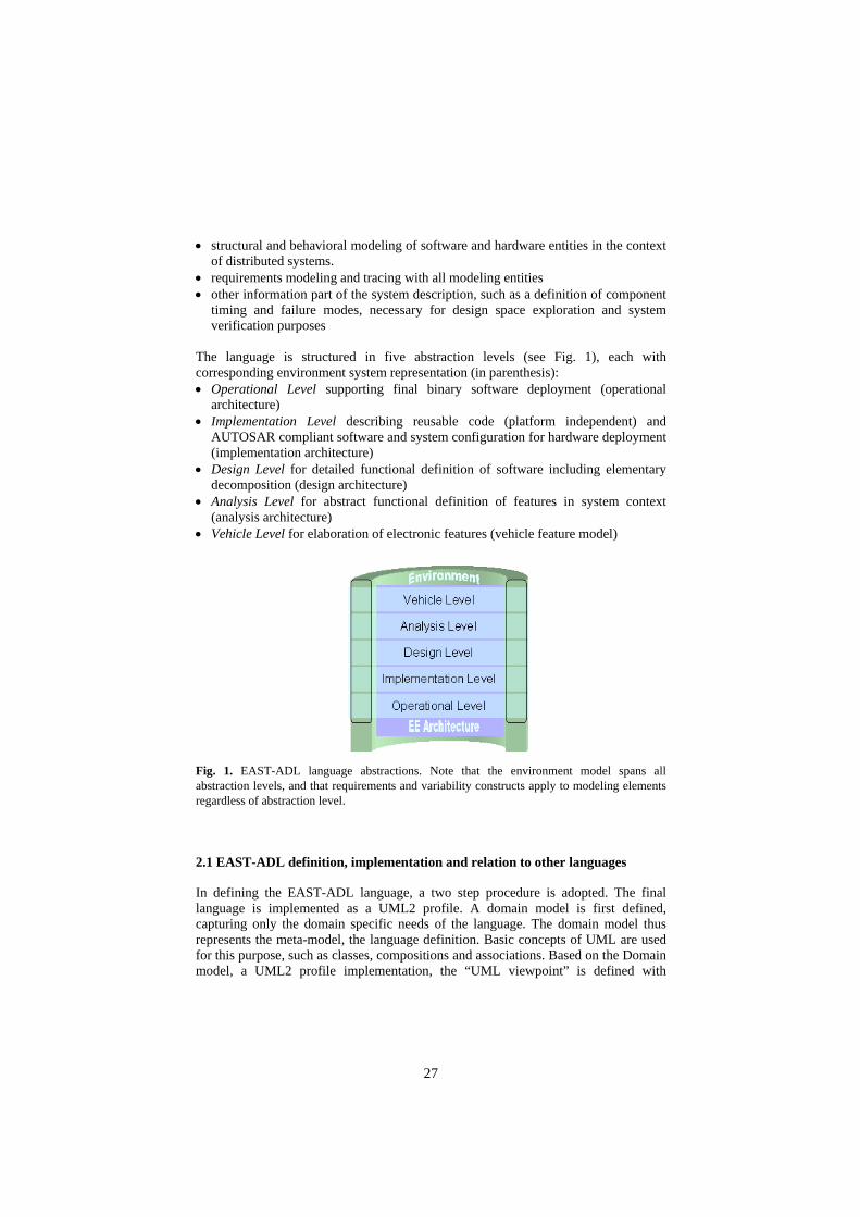
The language is structured in five abstraction levels (see Fig. 1), each with corresponding environment system representation (in parenthesis): • Operational Level supporting final binary software deployment (operational

architecture) • Implementation Level describing reusable code (platform independent) and

AUTOSAR compliant software and system configuration for hardware deployment (implementation architecture)

• Design Level for detailed functional definition of software including elementary decomposition (design architecture)

• Analysis Level for abstract functional definition of features in system context (analysis architecture)

• Vehicle Level for elaboration of electronic features (vehicle feature model)

Fig. 1. EAST-ADL language abstractions. Note that the environment model spans all abstraction levels, and that requirements and variability constructs apply to modeling elements regardless of abstraction level.

2.1 EAST-ADL definition, implementation and relation to other languages

In defining the EAST-ADL language, a two step procedure is adopted. The final language is implemented as a UML2 profile. A domain model is first defined, capturing only the domain specific needs of the language. The domain model thus represents the meta-model, the language definition. Basic concepts of UML are used for this purpose, such as classes, compositions and associations. Based on the Domain model, a UML2 profile implementation, the “UML viewpoint” is defined with

27

stereotypes, tags and constraints. This implementation is delivered as an XMI file ready for use in UML2 tools. As a proof-of-concept, an Eclipse based prototype tool with supporting analysis features, Papyrus [20], has been implemented. The EAST-ADL language also incorporates relevant aspects from SysML [14] and MARTE [9]. SysML is a modeling language that supports the specification, analysis, design, verification and validation of systems which may include hardware, software, information, processes, personnel, and facilities. SysML is defined in terms of a UML2 profile. MARTE is an ongoing effort to define a UML profile for Modeling and Analysis of Real-Time and Embedded systems, initiated to overcome the UML limitations of modeling such systems. The EAST-ADL is also being harmonized with the new automotive domain standardization AUTOSAR [18]. AUTOSAR focuses mainly on the implementation level of abstraction, whereas the EAST-ADL supports the overall comprehensive systems modeling.

Inspiration in the development of the EAST-ADL is also gathered from the SAE Architecture and Analysis Description Language (AADL) [16] and safety standards such as the ISO 26262 Functional Safety (committed draft planned for beginning 2008).

Considering the multitude of languages that in different ways address embedded systems, a relevant question is how the EAST-ADL relates to other modeling language efforts. This was partly elaborated in the previous text, but the main reasons for introducing “yet another language” are summarized here for clarity:

• EAST-ADL vs. UML: UML is a general modeling language for software engineering, which contains no specifics for automotive embedded systems. The EAST-ADL provides a tailoring of UML2 through a profile dedicated for such systems.

• EAST-ADL vs. SysML: SysML is a UML2 profile for systems engineering. EAST-ADL incorporates several SysML concepts and specializes them as needed for automotive embedded systems.

• EAST-ADL vs. AUTOSAR: AUTOSAR focuses on software and hardware implementation. The EAST-ADL complements AUTOSAR with e.g. functional specifications and requirements and reuses AUTOSAR concepts for the implementation level abstractions.

• Why not proven proprietary tools and languages such as MATLAB/Simulink [13], ASCET [5] or Modelica? The very fragmentation into multiple domain/discipline tools that target different aspects of the system is a key driver for developing the EAST-ADL. The EAST-ADL language provides an information structure for the engineering data required as a basis for automotive embedded systems development. In the ATESST project, interfaces in terms of model transformations and tool interfaces for the prototype tool Papyrus are developed to domain tools/languages.

• Why not information management tools such as product data management tools (PDM)? Such tools lack an information model for automotive embedded systems and the connections to external domain tools. The EAST-ADL domain model could be used as a basis for information management in existing PDM-like tools. Moreover, the use of UML2 allows native behavior to be defined. The fact that UML2 is a standard allows the EAST-ADL to be used with several UML tools.

28

2.2 Behavior modeling approach in EAST-ADL

With respect to behavior the goal of the EAST-ADL is to provide native behavior descriptions, for primitive components, as well as for compositions. Native behavior is useful for example to describe the desired overall behavior of the vehicle systems as well as the environment. The objective includes a native behavioral notation that allows simulation and verification within the defined system model, but also concerns the integration of external tools, as part of today’s industrial practice for designing behavior algorithms of vehicle applications. Integration here refers to the ability to import/export models to and from external tools based on model transformations.

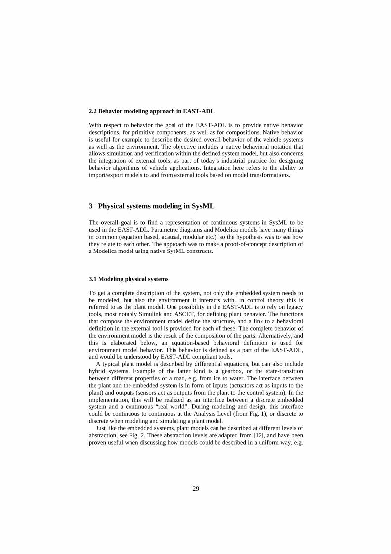
3 Physical systems modeling in SysML

The overall goal is to find a representation of continuous systems in SysML to be used in the EAST-ADL. Parametric diagrams and Modelica models have many things in common (equation based, acausal, modular etc.), so the hypothesis was to see how they relate to each other. The approach was to make a proof-of-concept description of a Modelica model using native SysML constructs.

3.1 Modeling physical systems

To get a complete description of the system, not only the embedded system needs to be modeled, but also the environment it interacts with. In control theory this is referred to as the plant model. One possibility in the EAST-ADL is to rely on legacy tools, most notably Simulink and ASCET, for defining plant behavior. The functions that compose the environment model define the structure, and a link to a behavioral definition in the external tool is provided for each of these. The complete behavior of the environment model is the result of the composition of the parts. Alternatively, and this is elaborated below, an equation-based behavioral definition is used for environment model behavior. This behavior is defined as a part of the EAST-ADL, and would be understood by EAST-ADL compliant tools.

A typical plant model is described by differential equations, but can also include hybrid systems. Example of the latter kind is a gearbox, or the state-transition between different properties of a road, e.g. from ice to water. The interface between the plant and the embedded system is in form of inputs (actuators act as inputs to the plant) and outputs (sensors act as outputs from the plant to the control system). In the implementation, this will be realized as an interface between a discrete embedded system and a continuous “real world”. During modeling and design, this interface could be continuous to continuous at the Analysis Level (from Fig. 1), or discrete to discrete when modeling and simulating a plant model.

Just like the embedded systems, plant models can be described at different levels of abstraction, see Fig. 2. These abstraction levels are adapted from [12], and have been proven useful when discussing how models could be described in a uniform way, e.g.

29

are the models on the same abstraction level, and can they be integrated on that level? There are also levels orthogonal to this, e.g. more or less advanced models, more or less validated models etc. These abstraction levels are not directly correlated to the EAST-ADL abstraction levels of the embedded system.

Fig. 2. Different levels of abstractions of environment models

Acausal models. At the highest level of abstraction for environment models, there are acausal models, where models are described by one or several differential or algebraic equations, possibly combined with state machines to model hybrid systems. The acausal Modelica components are on this level of abstraction, where equations and their relation to the outside world are modeled. Acausal models are generally more flexible and reusable than models at a lower abstraction level [6].

Causal models. At the causal level of abstraction, it is defined what is input, and what is output inside the system, and between components in a composed system. Typical causal models include bond graph representations [11], or block diagrams, like continuous Simulink models.

Time-discretized models. To solve a differential equation numerically it is typically discretized in time. A discretized model is an algorithmic representation in the sense that it generates a defined output for a certain input and internal state. A model can be discretized in different ways, e.g. using forward/backward Euler.

Simulation behavior. To perform the calculations of the discretized models, a solver and a scheduler is needed as part of the simulation engine. The simulation engine can decide the time-step, execution order, triggering, communication, etc. of the model. Typical numerical tools to solve differential equations are Simulink and ASCET [5]. Here, the simulation behavior of the continuous time model can be described using the same Model Of Computation (MOC) as for the model components of the embedded system.

Proceeding to lower abstraction levels means that the model gets more sophisticated, in the sense that the model can produce simulation results. On the other hand, the models get more specialized and differ more from the original system. Moreover, numerical errors could be introduced at all transformations. Tools and methods could use many of these abstraction levels, and hide some from the user. For example, a continuous Simulink model is modeled as a causal model. The choice of solver provides a way of (indirectly) discretizing the model since it implies a discrete-time implementation through the simulation behavior built into the tool. The Dymola [4] tool makes a point of taking the equations from the highest abstraction level to the

30

lowest, while ASCET uses models close to the lowest level, and letting the user have control over the real-time hardware-in-the-loop simulation.

3.2 SysML parametric diagrams

SysML consists of four behavioral and five structural diagrams. Seven of these diagrams are partially reused from UML, while two are new: the requirement diagrams and the parametric diagrams [14]. The parametric diagrams’ conceptual foundation is the composable objects representation (COBs), developed at Georgia Institute of Tecnology [10], the academic partner of the SysML team [14]. COBs provide five basic views of a system, Shape Schematic, Relations, Constraint Schematic, Lexical COB structure and Subsystem, of which Relations, Constraint Schematic and Subsystems have equivalent representation in parametric diagrams.

Parametric diagrams describe constraints between variables, like equations, and how they are related to each other. The SysML specification gives an example of Newtons equation, which can be modeled in continuous time [14]. The constraints are acausal, and by combining many modular subsystems, acausal relationships for a large system can be achieved. In addition, state machines can tell which equations to be used in the parametric diagrams, to be able to describe hybrid systems.

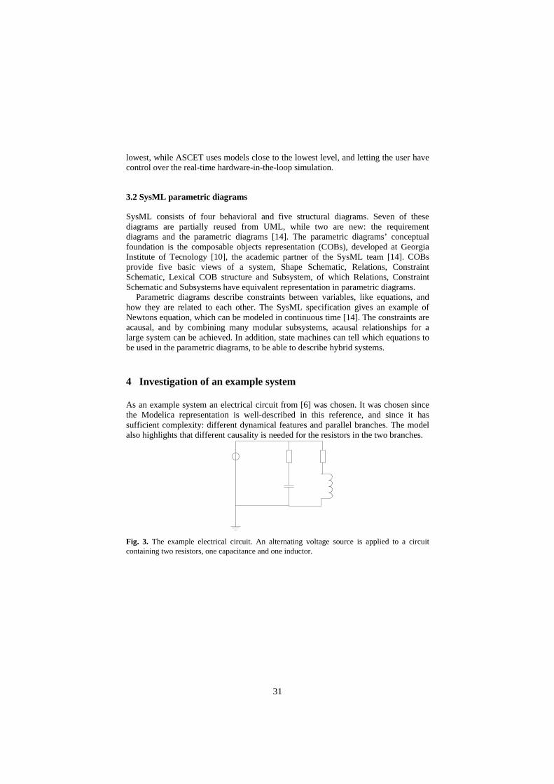
4 Investigation of an example system

As an example system an electrical circuit from [6] was chosen. It was chosen since the Modelica representation is well-described in this reference, and since it has sufficient complexity: different dynamical features and parallel branches. The model also highlights that different causality is needed for the resistors in the two branches.

Fig. 3. The example electrical circuit. An alternating voltage source is applied to a circuit containing two resistors, one capacitance and one inductor.

31

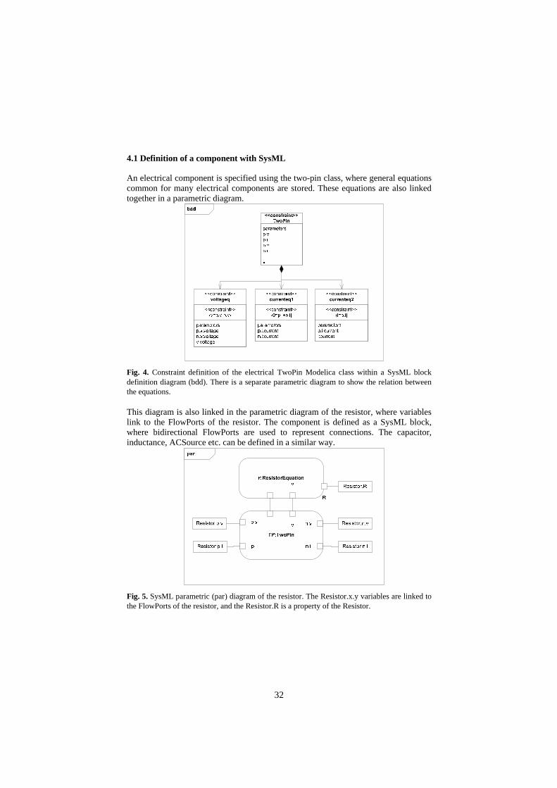
4.1 Definition of a component with SysML

An electrical component is specified using the two-pin class, where general equations common for many electrical components are stored. These equations are also linked together in a parametric diagram.

Fig. 4. Constraint definition of the electrical TwoPin Modelica class within a SysML block definition diagram (bdd). There is a separate parametric diagram to show the relation between the equations.

This diagram is also linked in the parametric diagram of the resistor, where variables link to the FlowPorts of the resistor. The component is defined as a SysML block, where bidirectional FlowPorts are used to represent connections. The capacitor, inductance, ACSource etc. can be defined in a similar way.

Fig. 5. SysML parametric (par) diagram of the resistor. The Resistor.x.y variables are linked to the FlowPorts of the resistor, and the Resistor.R is a property of the Resistor.

32

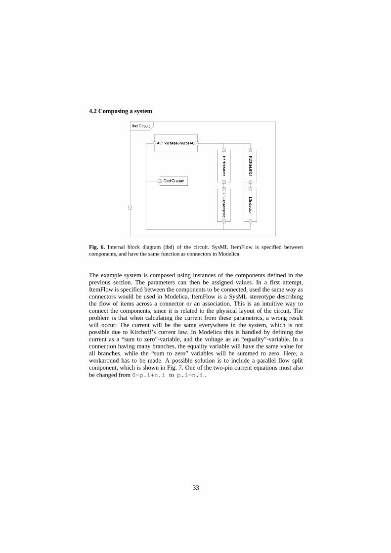
4.2 Composing a system

Fig. 6. Internal block diagram (ibd) of the circuit. SysML ItemFlow is specified between components, and have the same function as connectors in Modelica

The example system is composed using instances of the components defined in the previous section. The parameters can then be assigned values. In a first attempt, ItemFlow is specified between the components to be connected, used the same way as connectors would be used in Modelica. ItemFlow is a SysML stereotype describing the flow of items across a connector or an association. This is an intuitive way to connect the components, since it is related to the physical layout of the circuit. The problem is that when calculating the current from these parametrics, a wrong result will occur: The current will be the same everywhere in the system, which is not possible due to Kirchoff’s current law. In Modelica this is handled by defining the current as a “sum to zero”-variable, and the voltage as an “equality”-variable. In a connection having many branches, the equality variable will have the same value for all branches, while the “sum to zero” variables will be summed to zero. Here, a workaround has to be made. A possible solution is to include a parallel flow split component, which is shown in Fig. 7. One of the two-pin current equations must also be changed from 0=p.i+n.i to p.i=n.i .

33

ibd Circuit

AC: VoltageSourceAC

Gnd:Ground

Fl1:FlowSplit

Fl1:FlowSplit

Fig. 7. An acausal representation of the system, where the equations are fully

described by the underlying parametric diagrams

4.3 Block diagram model expressed as an activity diagram

The system could also be described at the causal level of abstraction. The circuit could be transferred to a bond graph representation. There are systematic approaches for electrical circuits, see for example [8]. Bond graphs could be described using SysML activity diagrams [15]. A bond graph model can also be converted to a block diagram [11], which could be expressed as an activity diagram, as described in [1]. This representation is shown in Fig. 8. To execute this diagram, initial values are needed on both “Add”-actions. When simulating a model in Simulink, the execution order is however typically not from input to output, it is decided by which blocks have direct-feed through and those that have internal state, see [13] for more information on this.

act

Voltagefunction

Add

Divide

R1Divide

C

Integrateover time

Negative

Add

Divide

LDivide

R2

Integrateover time

Negative

Output I1

Fig. 8. An activity diagram describing the circuit. This is similar to the Simulink representation, although the sequencing of the actions differ

34

5 Discussion and Conclusions

An attempt to make modular simulation models of physical systems using SysML has been tested and evaluated. The concepts includes internal block diagrams with attached parametric diagrams, bi-directional FlowPorts, and ItemFlow, The approach is maybe not the intended way to use these diagrams. The intention in SysML is to connect parametric diagrams to each other to generate a composed parametric diagram for the system. Then, the governing equations in this parametric diagram are separated from the structure in the internal block diagrams.

Although parametric diagrams are acausal, they do not contain any separation between effort and flow variables, which is fundamental when modeling physical systems [11]. Both Modelica (using flow) [6] and VHDL-AMS (using across/through) [7] contain such constructs. The solution of introducing the flow-split block is not an appealing solution; the point of using acausal diagrams is then somehow lost. Another solution would be to introduce stereotypes for flow variables, to show that they are to be summed to zero. A parametric diagram could be manually generated, or in principle automatically generated, based on the properties of the internal block diagram.

The behavior of the composed system could of course also be modeled using a non-modular parametric diagram. An optimized system model of the example system contains seven equations [6], which could easily be modeled using a single parametric diagram.

Using activity diagrams it is possible to model a block model version of the system. The activity diagram is a behavioral diagram, as opposed to the parametric diagrams (which are structural). This is a way to capture the structure of a Simulink model which is the causal representation of the system. This is an interesting path and will be further investigated in the ATESST project.

The compatibility between Modelica and UML representations needs further investigation. The advantage of having a Modelica compatible description is that it could be translated to Modelica models, and then simulated in existing Modelica tools.

Acknowledgements. This work has been carried out within the ATESST project, 2004-026976 in the EC 6th Framework Programme.

References

1. Bock, C., SysML and UML 2 Support for Activity Modeling, Wiley Interscience (2005) 2. Chen, D-J., Törngren, M., Shi, J., Årzen, K-E., Lönn, H., Gérard, S., Strömberg, M.,

Servat, D.. Model Based Integration in the Development of Embedded Control Systems – a Characterization of Current Research Efforts. In Proc. of the IEEE International Symposium on Computer-Aided Control Systems Design, Technische Universität München, Munich, Germany (2006)

3. Cuenot, P. Chen, D-J., Gérard, S., Lönn, H., Reiser, M-O., Servat, D., Tavakoli Kolagari, R., Törngren, M., Weber, M., Improving Dependability by Using an Architecture

35

Description Language. Accepted book chapter contribution for the forthcoming book /Architecting Dependable Systems IV/. Editors: Rogerio de Lemos, Cristina Gacek, Alexander Romanovsky. To be published by Springer, Lecture Notes in Computer Science series.

4. Dymola user manual, Dynasim AB, Lund, Sweden (2005) 5. ETAS Product and Service Catalog 2006/2007, ETAS GmbH, Stuttgart, Germany (2007) 6. Fritzson, P., Principles of Object-Oriented Modeling and Simulation with Modelica 2.1,

IEEE Press, Wiley-Interscience (2004) 7. Heinkeel, U. et al., The VHDL Reference, John Wiley, England (2000) 8. Ljung, L. & Glad, T., Modellbygge och simulering, Studentlitteratur, Lund, Sweden

(1991) 9. Object Management Group: UML Profile for Modeling and Analysis of Real-Time and

Embedded systems (MARTE), RFP. (2005) 10. Peak, R.S., Burkhart, R.M., Friedenthal, S.A., Wilson, M.W., Bajaj, M., Kim, I.,

Simulation-Based Design Using SysML—Part 1: A Parametrics Primer. INCOSE Intl. Symposium, San Diego (2007)

11. Rosenberg, D.L., Margolis, D.L., Karnopp, D.C, System dynamics : modeling and simulation of mechatronic systems, Wiley, New York, N.Y. (2000)

12. Sen, S., Vangheluwe, H., Multi-Domain Physical System Modeling and Control Based on Meta-Modeling and Graph Rewriting, proceedings of the 2006 IEEE Conference on Computer Aided Control Systems Design, Munich, Germany (2006)

13. Simulink user manual, MATLAB release 2006b, Mathworks (2006) 14. SysML Specification v1.0, SysML partners (2006) 15. Turki, S. & Soriano, T., A SysML extension for Bond Graphs support, 5th International

Conference on Technology and Automation (ICTA’05) (2005) 16. www.aadl.info 17. www.atesst.org 18. www.autosar.org 19. www.east-eaa.net 20. www.papyrusuml.org

36

Hybrid Dynamics in Modelica: Should all Events be

Considered Synchronous

Ramine Nikoukhah

INRIA-Rocquencourt, BP 105, 78153 Le Chesnay Cedex.

Email: ramine.nikoukhah@inria.fr

Abstract. The Modelica specification is ambiguous as to whether all the events

are synchronous are not. Different interpretations are possible leading to

considerable differences in the ways models should be constructed and

compilers developed. In this paper we examine this issue and show that there

exists an interpretation that is more appropriate than others leading to more

efficient compilers. It turns out that this interpretation is not the one currently

adopted by Dymola but it is closely related to the Scicos formalism.

Keywords: Modelica, Synchronous language, Scicos, modeling and simulation.

1 Introduction

Modelica (www.modelica.org) is a language for modeling physical systems. It has been

originally developed for modeling systems obtained from the interconnection of

components from different disciplines such as electrical circuits, hydraulic and

thermodynamics systems, etc. These components are represented symbolically in the

language providing the compiler the ability to perform symbolic manipulations on the

resulting system of differential equations. This allows the usage of acausal components

(equation based) without loss of performance.

But Modelica is not limited to continuous-time models [1]; it can be used to construct

hybrid systems, i.e., systems in which continuous-time and discrete-time components

interact. Modelica specification [2] tries to define the way these interactions should be

interpreted and does so by inspiring from the formalism of synchronous languages.

Synchronous languages however deal with events, i.e., discrete-time dynamics. So in the

context of Modelica, the concept of synchronism had to be extended to encompass

continuous-time dynamics as well. It is exactly this extension which is the subject of

this paper.

Scicos (www.scicos.org) is a modeling and simulation environment for hybrid systems.

It is free software, included in the scientific software package Scilab (www.scilab.org).

Scicos formalism is based on the extension of synchronous languages, in particular

Signal [3], to the hybrid environment. The class of models that Scicos is designed for is

almost the same as that of Modelica. So it is not a surprise that Modelica and Scicos

37

have many similar features and confront similar problems. Modelica has many

advantages for modeling continuous-time dynamics, especially thanks to its ability to

represent models in symbolic form, whereas the Scicos formalism has been specifically

designed to allow high performance code generation of discrete-time dynamics.

In this paper, we examine the specification of hybrid dynamics in Modelica and propose

an interpretation that is fully compatible with the Scicos formalism. This interpretation,

which is not contradictory with the official specification, allows us to obtain an efficient

compiler/code generator for Modelica inspired by the Scicos compiler.

Here we start with a flat model (obtained from the application of a front-end compiler),

and consider only the problems concerning the design of the phase one of a back-end

compiler. This phase breaks down the code into independent asynchronous parts each of

which can be compiled separately in phase two. Phase two will be presented in a

subsequent paper.

2 Conditioning and Sub-sampling in Modelica

If a model contains no conditioning and all of its parts function at the same rate, then

back-end compilation would be a simple task. But in most real life applications, models

contain different dynamics resulting from the inter-connection of heterogeneous

systems. A model of such a system would often include conditioning and sub-sampling.

We use the term conditioning for a change in the model conditioned on the value of a

variable (for example if a>0 then) and the term sub-sampling for the construction of a

new, not necessarily regular, clock from a faster clock.

The when-elsewhen and if-then-else clauses are the basic language constructs in

Modelica for performing conditioning and sub-sampling. The description of the ways

these constructs function is ambiguous in the Modelica specification. Comparing with

the Scicos formalism, we can consider that Modelica’s if-then-else clause does

conditioning and when does sub-sampling. But the situation is somewhat more complex

because when plays two different roles. And, we need to distinguish these two different

types of when clauses. But before, we need to examine the notion of synchronism in

Modelica.

2.1. Synchronous versus Simultaneous

In our interpretation of the Modelica specification, two events are considered

synchronous only if they can be traced back to a single event source. For example in the

following model:

when sample(0,1) then

d=pre(d)+1;

end when;

when d>3 then

a=pre(a)+1;

end when;

the event d>3 is synchronous with the event sample(0,1). The former is the source of

the latter. But in

38

der(x)=x ;

when sample(0,1) then

d=pre(d)+1;

end when;

when x>3 then

a=pre(a)+1;

end when;

the two events are not synchronous. There is no unique source of activation at the origin

of these events. So these events are considered asynchronous even if the two events are

activated simultaneously; even if we can prove mathematically that they always occur

simultaneously.

Our basic assumption is that events detected by the zero-crossing mechanism of the

numerical solver (or an equivalent mechanism used to improve performance) are always

asynchronous. So even if they are detected simultaneously by the solver, by default they

are treated sequentially in an arbitrary order. In particular, in the model:

when sample(0,1) then

b=a;

end when;

when sample(0,1) then

a=b+1;

end when;

the variables a and b can be evaluated in any order.

Dymola on the other hand assumes that all events are synchronous. In particular it

assumes that all the equations in both when clauses may have to be satisfied

simultaneously. That is why Dymola finds an algebraic loop in this example.

To see the way Dymola proceeds, consider the following example:

equation

der(x)=1;

der(y)=1;

when (x>2) then

z=pre(z)+3;

v=u+1;

end when;

when (y>2) then

u=z+1;

end when;

The simulation shows that the equations (assignments) are ordered as follows:

z=pre(z)+3;u=z+1;v=u+1;

this means that the content of a when clause is split into separate conditional clauses. In

stark contrast, in our interpretation of the Modelica specification, the code within an

asynchronous when clause is treated synchronously and never broken up. Both

interpretations are valid and consistent; however our interpretation has many advantages

as we will try to show here.

At first glance, the non determinism that may be encountered in our approach when two

zero-crossing events occur simultaneously may seem unacceptable. However, treating

two simultaneous zero-crossings as synchronous is not a solution because it is not

robust. Indeed, when dealing with nonlinear and complex models, there is no guarantee

that the numerical solver would detect two zero-crossings simultaneously even if

39

theoretically they are simultaneous. In general one is detected slightly before or after

the other. And in any case, in most cases treating such an accidental synchronism is not

of any use for the construction of the model. Even if the model depends for some reason

on the simultaneous detection of two events by the solver, a mechanism should be

provided by the language to specify explicitly what should be done in that case. One

way would be to introduce a switchwhen clause [4], which can be used to explicitly

specify what equations are activated in every possible case. The possible cases when we

have, for example, two zero-crossings are: the first surface has crossed but not the

second, the second has crossed but not the first and finally both surfaces have crossed

zero together.

Dymola’s interpretation imposes constraints, which in most cases are useless. Moreover,

when all zero-crossing events are considered synchronous, the complexity of static

scheduling increases with the number of zero-crossings. The solution based on using the

switchwhen clause allows the user to specify explicitly what possible synchronisms must

be considered. It turns out that in most cases, no synchronism is to be considered.

2.2. Primary and Secondary when Clauses

So far we have seen two types of when clauses, or more specifically when clauses based

on two types of events: events depending on variables evolving continuously in time

such as time>3 or x<2 where x is a continuous variable; and events depending on

discrete variables. when clauses conditioned on events of the former type are called

primary, the latter ones are called secondary.

An event associated with a secondary when clause is necessarily synchronous with

events associated to one or more primary when clauses. These primary clauses are

those in which the discrete variables involved in the definition of the event are defined.

But not all when clauses can easily be classified as primary or secondary. Let us

consider a simple example:

when sample(0,1) then

d=pre(d)+j;

c=b;

end when;

when time>d then

b=a;

end when;

The question is whether or not the above two when clauses are primary or not. Clearly

the first one is, but the second hides in reality two distinct when clauses that is because

the event time>d can be activated in two different ways:

• time increases and crosses d continuously (zero-crossing event so asynchronous),

• at a sample time d jumps, activating the time>d condition; this event is clearly

synchronized with sample(0,1).

We call such when clauses mixed. We handle this situation by implementing the

simulation in such a way that time>d is activated only when time crosses continuously d

and placing a duplicate of the content of this when where d is defined within a condition

that guarantees that the content is activated only if time>d is activated due to a jump:

when sample(0,1) then

40

d=pre(d)+j;

c=b;

if ((time>d) and not(time>pre(d))) then

b=a ;

end if ;

end when;

when time>d then

b=a;

end when;

The second solution amounts to considering that a clause such as when c>0 where c is a

continuous variable is activated only if c crosses zero continuously (the way that is

detected by zero-crossing mechanisms built into numerical solvers such as LSODAR or

DASKR). This seems to be an appropriate way to handle mixed when clauses, however

to stay compatible with the Modelica specification, at a pre-compilation phase, the

content of these clauses must be duplicated as explained above.

Note that the code we obtain after the pre-compilation phase is not correct according to

the Modelictcification (because b is defined twice). This however is not a problem

because this code is only used within the compiler. But in any case, we consider this

restriction too restrictive and we think it should be relaxed. This will be discussed later.

There still remains a situation that needs clarification. Consider the following example:

discrete Real a(start=0);

Real x(start=0);

equation

der(x)=0;

when x>3 then

a=pre(a)+1;

end when;

when time>2 then

reinit(x,x+4);

end when;

Here x is a continuous variable, but it is also discrete because at time 2 it jumps from 0

to 4 (activation of reinit). This jump activates the content of the first when. The reinit

primitive in this case must be considered as a definition of “discrete” x, so following the

rule discussed previously, the content of the clause when x>3 must be copied inside the

other when:

discrete Real a(start=0);

Real x(start=0);

equation

der(x)=0;

when x>3 then

a=pre(a)+1;

end when;

when time>2 then

reinit(x,x+4);

if edge(x>3) then

a=pre(a)+1;

end if ;

end when;;

This transformation is just a special case of the situation we have considered previously.

To see this more clearly, note that

41

when time>2 then

reinit(x,x+4);

end when;

should really be expressed as follows:

when time>2 then

x=pre(x)+4;

end when;

2.3. Restrictions on the Use of when and if

Modelica imposes hard constraints on the usage of when and if-then-else clauses.

In the case of when, a variable is not allowed to be defined in two when clauses. For

example the following code is not allowed in an equation section:

when sample(0,1) then

b=pre(b)+1 ;

end when ;

when time>3.5 then

b=0 ;

end when ;

According to the specification, this can lead to a contradiction if the two when clauses

are activated at the same time. This statement would make sense if the two when clauses

were synchronous but not in this case. Lifting this restriction, in the case of primary

when clauses, is without danger and facilitates the task of modeling in many situations.

However, it creates an important difference as far some interpretation of the primitive

pre is concerned. With the current restriction, we are sure that in the following code:

when sample(0,1) then

b=pre(b)+1 ;

end when;

pre(b) is the previous value of b defined by b=pre(b)+1 the last time this when clause

was activated, i.e. one unit of time before. So without even having to examine the rest

of the code, we can be sure that b indicates the time. This will no longer be true if the

constraint is lifted; consider:

when sample(0,1) then

b=pre(b)+1 ;

end when;

when sample(.5,1) then

b=pre(b)+1 ;

end when;

In this case the value of b used to update it in each clause is computed by the instruction

in the other clause. But this is not a problem as long as the rules are clear.

We thus propose the following modifications: this restriction be lifted for primary when

clauses and this restriction be lifted in all when clauses as long as the equations defining

common variables are identical (such identical equations can arise in transformations

applied by the compiler which includes duplicating parts of the code). For example for

all conditions c1, c2 (synchronous or not), accept:

equation

42

when c1 then

b=a;

end when;

when c2 then

b=a;

end when;

The second modification may seem strange. Indeed why would a model contain

identical statements in synchronous when clauses. The reason is that our Modelica

compiler performs a series of transformations each one generating a new Modelica code

from a Modelica code in which such a situation may come up (this happens in particular

when processing the union of events construct, see Section 2.6). By lifting this

restriction, we make sure that we obtain a valid Modelica code at every stage. But a

specific test must be applied to the original model to issue at least a warning to the user

for such cases.

Another important restriction concerns the use of elsewhen. The Modelica specification

states that all the branches of a when-elsewhen clause must define the same set of

variables. We don’t believe this constraint is justified. This constraint is probably a

consequence of a similar condition on the use of if-then-else clauses. Indeed Modelica

imposes that the number of equations in different branches of such a clause be identical.

This may be acceptable as far as continuous-time variables are concerned1, but it is not

for discrete variables. So we propose to lift this restriction and accept models including

for example the following code:

equation

when sample(0,1) then

if u>0 then

v=1;

end if;

end when;

Normally in Modelica we should have an else branch defining v. Note that our proposal

is not just an editing facility (i.e., a way to avoid writing code which can be added in

automatically later); this code is not equivalent to

equation

when sample(0,1) then

if u>0 then

v=1;

else

v=pre(v) ;

end if;

end when;

In the absence of the else branch, the variable v is sub-sampled. This would not be the

case if v=pre(v) were used. Even if the simulation result would be the same, the

construction by sub-sampling leads to the generation of more efficient code. Lifting this

restriction is again important for transformed models. A specific test can be used on the

original model to impose the constraint if desired.

1 Removing the restriction in the continuous case makes it possible to model Simulink’s

enabled Super Blocks in Modelica.

43

2.4. Continuous-Time Dynamics

Our objective is to reduce the Modelica code into a number of asynchronous when

clauses each of which can be treated separately. The continuous dynamics is no

exception. What we call continuous dynamics includes everything within the equation

section but outside when clauses. These equations are always active (Scicos

terminology) even when a when clause is activated. So these equations are synchronous

with all the when clauses.

The way this situation is handled in Scicos is to introduce a fictitious clock generating a

continuous activation signal. To do the same in Modelica amounts to defining a special

when clause:

when continuous then

the content of which would be active all the time except at event instances associated to

other when clauses. Doing so allows us to consider the “continuous” event as

asynchronous with the rest and treat this when clause as primary. To preserve the

dynamics of the original model, the continuous dynamic equations must also be copied

inside all the when clauses. For example:

equation

y=sin(time) ;

der(x)=y ;

when x<.2 then

a=y ;

end when ;

becomes

equation

when continuous then

y=sin(time) ;

der(x)=y ;

end when ;

when x<.2 then

y=sin(time) ;

der(x)=y ;

a=y ;

end when ;

During the simulation, the content of the when continuous clause is used to respond to

the queries of the numerical solver, and in particular to generate the value of der(x) in

this case. In other when clauses, the equations defining derivative values can be

dropped, especially in the explicit case. In the implicit case (DAE case), the

computation of the derivatives can be used to help the re-initialization of the solver.

The point to retain from this section is that the clause when continuous is primary and

that its content can be treated like any other.

2.5. Initial Conditions

In Modelica, variables can be initialized in different ways but in a flat model (after the

application of the front end), they should all be grouped within a single when clause:

when initial then

44

a=0 ;

d=3 ;

…

end when ;

This would be a primary when clause and would contain the initialization of all discrete

and continuous variables.

A when terminal clause can similarly be used to specify whatever needs to be done at

the end of the simulation.

2.6. Union of Events

The when and elsewhen clauses can be activated at the union of events. In Modelica the

syntax is as follows:

when c1,c2,c3 then

< eq1 >

< eq2 >

end when;

In this case, c1, c2, c3 may be synchronous or not. Note that the content of synchronous

when clauses should not be executed more than once. For example in:

when sample(0,1) then

d=pre(d)+1;

end when;

when d>2,2*d>4 then

a=pre(a)+1 ;

end when;

a must be incremented only once, passing from zero to one. But in:

when sample(0,1) then

d=pre(d)+1;

end when;

when sample(0,1) then

e=pre(e)+1;

end when;

when d>2,e>2 then

a=pre(a)+1 ;

end when;

a is incremented twice (its value must jump from zero to two). But Dymola considers

the d>2 and e>2 synchronous and increments a just once in this case. Similarly in:

when sample(0,3) then

d=pre(d)+1;

end when;

when time>=3 then

e=pre(e)+1;

end when;

when d>1,e>0 then

a=pre(a)+1 ;

end when;

in Dymola d>1, e>0 are synchronous (a is incremented only once at time 3). As we

have said previously, we think that this interpretation must be avoided.

45

The counterpart of the union of events is the sum of activation signals in Scicos. The

two formalisms coincide perfectly in this case.

In one of the early phases of the compilation of Modelica code, we propose the

following transformation which removes all event unions. For example the first when

clause presented in this section would be transformed as follows:

when c1 then

< eq1 >

< eq2 >

end when;

when c2 then

< eq1 >

< eq2 >

end when;

when c3 then

< eq1 >

< eq2 >

end when;

This code is correct if we take into account all the modifications suggested previously

whether the ci, i=1,2,3, are synchronous or not.

3 Back-end Compiler

The back-end compiler can be divided into two phases. The objective of the first phase

is to transform the model into one in which all the when clauses are primary. This will

allow us to generate, in phase two, static code for each one independently of the others.

Consider the following example:

when time>3 then

d=pre(d)+1;

end when;

when d>3 then

a=pre(a)+1;

end when;

when a>3 then

b=a;

end when;

We want to remove the secondary when clauses. Clearly in this case we have to remove

the last two when clauses. We pick one (say when a>3) and copy its content everywhere

the variables involved in the definition of the corresponding event are computed. In this

case the only variable involved is a, which is defined in the second when clause:

when time>3 then

d=pre(d)+1;

end when;

when d>3 then

a=pre(a)+1;

if edge(a>3) then

b=a;

end if ;

46

end when;

and then

when time>3 then

d=pre(d)+1;

if edge(d>3) then

a=pre(a)+1;

if edge(a>3) then

b=a;

end if ;

end if ;

end when;

This example shows how secondary when clauses can be removed to obtain a single

primary when clause at the end. If the model contains more than one primary when

clause, the procedure would still be the same as illustrated in the following example:

when time>2 then

a=1 ;

end when ;

when time>3 then

b=pre(b)+1 ;

end when ;

when a>b then

c=1 ;

end when ;

In this case the first two when clauses are primary. We now remove the secondary when:

when time>2 then

a=1 ;

if edge (a>b) then

c=1 ;

end if ;

end when ;

when time>3 then

b=pre(b)+1 ;

if edge (a>b) then

c=1 ;

end if ;

end when ;

In this example, a variable is defined twice in two different primary (so asynchronous)

when clauses. Clearly, this is not a problem. But the application of the transformation,

can also lead to a variable being defined more than once in the same when clause. Let us

examine the following example:

when time>2 then

a=pre(a)+1 ;

end when ;

when a>d then

b=pre(b)+1 ;

end when ;

when a>2,b>2 then

n=pre(n)+1 ;

end when ;

47

We start by removing the operator “union of events. Then we remove the secondary

clauses as previously described. We obtain (in two steps):

when time>2 then

a=pre(a)+1 ;

if edge(a>d) then

n=pre(n)+1 ;

end if ;

if edge(a>2) then

b=pre(b)+1 ;

if edge(b>2) then

n=pre(n)+1 ;

end if ;

end if ;

end when ;

This code, once edge replaced with its definition, may seem to be ordered properly and

usable as a sequential code. But this is not the case since n=pre(n)+1, in some cases,

can be executed twice instead of once. As discussed in the previous section, it is

allowed to have a variable defined twice synchronously as long as the equations

defining it are identical. This is of course the case here (this is the case in general when

it happens because of the application of our transformations).The second phase of the

compilation will transform the code into a sequential code correctly.

4 Conclusion

We have examined the notion of synchronism in Modelica and have shown that by

abandoning the fully synchronous assumption, it is possible to design more efficient

compilers without loss of rigor in the language specification. We have done that by

proposing a methodology to implement the first phase of a back-end compiler. The

second phase, which is closely related to the second phase of the Scicos compiler, will

be presented in a future.

References

1 M. Otter, H. Elmqvist, S. E. Mattsson, “Hybrid Modeling in Modelica based on the

Synchronous Data Flow Principle”, CACSD’99, Aug; 1999, Hawaii, USA.

2 Modelica Association, “Modelica - A Unified Object-Oriented Language for Physical

Systems Modeling. Language Specification, version 2.2”, 2005, available from

www.modelica.org/.

3 A. Benveniste, P. Le Guernic, C. Jacquemot.,"Synchronous programming with events and

relations : the Signal language and its semantics", Science of Computer Programming, 16,

1991, p. 103-149.

4 R. Nikoukhah, “Extensions to Modelica for efficient code generation and separate

compilation”, in Proc. EOOLT Workshop at ECOOP’07, Berlin, 2007.

5 P. Fritzson - “Principles of Object-Oriented Modeling and Simulation with Modelica 2.1”,

Wiley-IEEE Press, 2003.

6 S. L. Campbell, Jean-Philippe Chancelier and Ramine Nikoukhah, “Modeling and

Simulation in Scilab/Scicos”, Springer, 2005.

48

Extensions to Modelica for efficient code generation and

separate compilation

Ramine Nikoukhah

1 INRIA-Rocquencourt, BP 105, 78153 Le Chesnay Cedex.

Email: ramine.nikoukhah@inria.fr

Abstract. In the current Modelica specification, the only admitted external

entities are memory-less functions. We propose an extension to allow parts of

the model containing internal states, conditioning and discrete dynamics, to be

definable as external functions. This opens the door to separate compilation of

Modelica code. For this purpose, we introduce the language construct

switchwhen and the type Event. These extensions are directly inspired by the

Scicos formalism.

1 Introduction

Modelica (www.modelica.org) is a language for modeling physical systems. It has been

originally developed for modeling systems obtained from the interconnection of

components from different disciplines such as electrical circuits, hydraulic and

thermodynamics systems, etc. Modelica can also be used to construct hybrid systems,

i.e., systems in which continuous-time and discrete-time components interact. With that

respect, Modelica is similar to Scicos (www.scicos.org), a modeling and simulation

environment for hybrid systems. Scicos is included in the free open-source scientific

software package Scilab (www.scilab.org). Modelica specifications are provided in an

official document; the current version is available in [1].

Unlike Scicos, in which model components are defined as grey-box modules (blocks),

the Modelica language requires that the complete model be expressed in the Modelica

language (except for simple memory-less external functions). It is currently virtually

impossible to isolate a sub-model and compile it separately or develop it in a different

language. But this is exactly what is needed when simulation environments are used to

design, validate and generate code for real-time applications.

This limitation in Modelica may seem surprising, especially when compared to Scicos.

Contrary to Modelica, the Scicos compiler requires only some macroscopic information

about each block (direct input/output dependency, presence of state, etc.; see [4] for

more information on Scicos block structure). The detail of the algorithm used within

each block is irrelevant to the compiler; the internal of each block is fully isolated from

the outside. A similar mechanism to isolate a sub-model does not exist in Modelica. In

this paper, inspired by the Scicos formalism, we propose a solution to this problem. This

is particularly important for applications where real-time code generation is sought. In

addition, it allows a harmonious integration of the two environments Modelica and

Scicos.

49

2 Language Extensions

The when-elsewhen and if-then-else clauses are the language constructs in Modelica for

performing conditioning and sub-sampling. We present extensions to these clauses,

which not only facilitate programming in Modelica, but also in conjunction with the

introduction of a new type, Event, allows for module isolation and separate compilation.

2.1. switch and swithwhen

The switch construct is a very natural extension of if-then-else:

switch (n)

case 1 :

< eq1 >

< eq2 >

…..

case 2 :

< eq3 >

< eq4 >

…..

case default:

< eq5 >

< eq6 >

…..

end switch;

One and only one case is active depending on the value of the integer n. The counterpart

in Scicos of this construct is realized with the ESelect block.

The switchwhen construct generalizes when-elsewhen.

switchwhen c1,c2,c3

case ‘001’ :

< eq1 >

< eq2 >

…..

case ‘010’ :

< eq3 >

< eq4 >

…..

case ‘111’:

< eq5 >

< eq6 >

…..

end switchwhen;

The content of one and only one case is activated depending on what combination of

events c1, c2 and c3 is generated. For example if events c1 and c3 are simultaneously

generated but not c2, then the case ‘101’ is activated. For this to happen, c1 and c2 must

be synchronous or be time events which are simultaneously detected (for example by the

zero-crossing mechanism of the numerical solver).

50

In most cases, simultaneous detection of time events (e.g. zero-crossings) needs not be

considered as a special case. By default, time events are considered asynchronous, in

case of “accidental” simultaneous detection, one event can usually be activated after

another (no specified order). For special cases where simultaneous detection does

matter, the switchwhen construct allows us to take advantage of this additional

information. This is useful in some applications as we shall see in the next example:

Example of Usage of switchwhen

Consider the problem of contact between three balls:

Ignoring the possibility of simultaneous contact, the dynamics of this system can be

modeled as a 1D problem as follows:

equation

der(x1)=v1;der(x2)=v2;der(x3)=v3;

der(v1)=0;der(v2)=0;der(v3)=0;

when x3-x1<=1 then

reinit(v1,pre(v3));

reinit(v3,pre(v1));

end when;

when x3-x2<=1 then

reinit(v2,pre(v3));

reinit(v3,pre(v2));

end when;

Here xi, i=1,2,3, denote the positions of the balls and we suppose that the balls 1 and 2

situated on left come into contact with the ball number 3 positioned on the right.

The simulation result shows that in the case of simultaneous contact, the model is

incorrect. The reason is that after a double contact, after treating one, the jump in the

speeds of the balls make it so that the second contact never happens. But this contact is

already detected and must be treated. This problem can be avoided by adding a test to

make sure that after treating the first contact, the result is taken into account before

treating the second:

when x3-x1<=1 then

if v1>v3 then

reinit(v1,pre(v3));

reinit(v3,pre(v1));

end if;

end when;

when x3-x2<=1 then

if v2>v3 then

reinit(v2,pre(v3));

reinit(v3,pre(v2)); end if;

51

end when;

This solution is consistent but it is not very flexible. In particular, it does not allow us to

specify explicitly what should happen in the case of a double contact. Using

switchwhen, the dynamics of simultaneous contact can be explicitly expressed:

equation

der(x1)=v1;der(x2)=v2;der(x3)=v3;

der(v1)=0;der(v2)=0;der(v3)=0;

switchwhen x3-x1<=1,x3-x2<=1 then

case “10”:

reinit(v1,pre(v3));

reinit(v3,pre(v1));

case “01”:

reinit(v2,pre(v3));

reinit(v3,pre(v2));

case “11”:

<TO DO IN CASE OF SIMULATANEOUS CONTACT>

end switchwhen;

We are not suggesting that switchwhen is a universal solution to the problem of contacts

in mechanics, which is a difficult problem in general. This example was simply chosen

to illustrate the usage of switchwhen in case of time events.

The most important use of switchwhen is for module isolation and applies to the case of

synchronous events as we shall see later.

2.2. Type Event and Primitive event

Currently events in Modelica are coded by Booleans:

e=edge(time>2) ; e=sample(0,1) ;

But these Booleans are not “normal” Booleans: they are of impulsive type. We can

consider then that events are coded by this type of Booleans. However, the edge

operator, which is usually used to generate events, does not always generate this type of

Boolean. For example if k is a discrete variable, then

when k>0 then

c=edge(b) ;

generates a “standard” Boolean. This shows that the edge does not always produce an

impulsive Boolean (as the name suggests). In fact, edge(b) is not just a function of b, it

depends on the argument of the when clause in which it is placed.

We see that there is no real distinction between a “standard” Boolean and one that is

used as an event. This can be very confusing as it can be seen in the following example:

discrete Real d,k;

Boolean b,c;

52

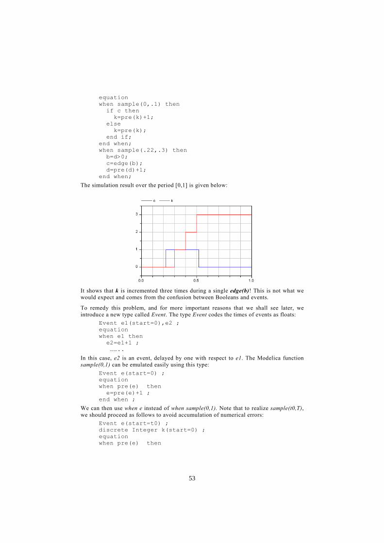
equation

when sample(0,.1) then

if c then

k=pre(k)+1;

else

k=pre(k);

end if;

end when;

when sample(.22,.3) then

b=d>0;

c=edge(b);

d=pre(d)+1;

end when;

The simulation result over the period [0,1] is given below:

It shows that k is incremented three times during a single edge(b)! This is not what we

would expect and comes from the confusion between Booleans and events.

To remedy this problem, and for more important reasons that we shall see later, we

introduce a new type called Event. The type Event codes the times of events as floats:

Event e1(start=0),e2 ;

equation

when e1 then

e2=e1+1 ;

……..

In this case, e2 is an event, delayed by one with respect to e1. The Modelica function

sample(0,1) can be emulated easily using this type:

Event e(start=0) ; equation

when pre(e) then

e=pre(e)+1 ;

end when ;

We can then use when e instead of when sample(0,1). Note that to realize sample(t0,T),

we should proceed as follows to avoid accumulation of numerical errors:

Event e(start=t0) ;

discrete Integer k(start=0) ;

equation

when pre(e) then

53

k=pre(k)+1 ;

e=k*T+t0 ;

end when ;

Events can also be generated from zero-crossings. We need a mechanism to generate

such Events. We have seen that the edge operator is not fully appropriate, that is why we

propose a new operator: event.

Event e1,e2;

……

equation

der(x)=sin(x);

e1=event(x>.2) ;

when e1 then

d=pre(d)+1 ;

e2=event(d>4);

end when ;

when e2 then

<xxx>

end when ;

Note that the two event operators in the above code both generate Events, but the

mechanism by which they do it is very different. The first one is used outside a when

clause, so it is realized in the compiler/simulator by the zero-crossing detection

mechanism of the numerical solver. The second on the other hand is inside a when, it is

synchronous and will be removed in the compilation phase. In this case this is done as

follows:

Event e1;

……

equation

der(x)=sin(x);

e1=event(x>.2) ;

when e1 then

d=pre(d)+1 ;

if (d>4) and not (pre(d)>4) then

<xxx>

end if ;

end when ;

The use of the type Event clarifies the situation to a point that we propose that only

Events be allowed as arguments of when clauses1. For example the 3 ball problem

introduced previously would be expressed as follows:

equation

der(x1)=v1;der(x2)=v2;der(x3)=v3;

der(v1)=0;der(v2)=0;der(v3)=0;

E1= event(x3-x1<=1);

E2=event(x3-x2<=1);

switchwhen E1,E2 then

case “10”:

….

1 This can be done gradually to reduce the problems of backward compatibility.

54

3 Applications

In this section we examine the applications of using the proposed extensions.

3.1. Compiler/Simulator Simplification

The ability to manipulate event times explicitly simplifies model construction. In

particular there is no need to use artificial tests against time. For example, consider the

problem of modeling the propagation delay in a digital circuit, which requires a variable

dependent event delay. This type of delaying operation can be realized as follows:

when time>c_time then

d_time=c_time+u;

end when;

when time>d_time then

…..

But using Event, the code can be made simpler:

when c_time then

d_time=c_time+u;

end when;

when d_time then

…..

But representing events explicitly, also simplifies the job of the compiler. In particular,

the compiler no longer needs to “figure out” what “tests” are simple enough to be

implemented without using the solver’s zero-crossing mechanism.

Another simplification comes from the canonical representation of the model when

Events are explicitly identified (declared) and used in conditioning of the when

statements. Consider the following example:

Event e1,e2,e3,…;

…….

equation

……

e1=event(…

when initial then

….

end when;

when e1 then

k=pre(k)+1;

e2=event(k>1);

….

when e2 then

e3=time+1;

….

end when;

…..

In this model, we can readily identify the Events and their types. Clearly e1 and e3 are

asynchronous Events; the first one is of type zero-crossing. But e2 is synchronous and

thus can be eliminated. This simplifies the task of the compiler, which in the first phase

55

of the compilation, removes e2 yielding a model containing only primary when clauses

(see [2] for the definition of a primary when clause):

Event e1,e3,…;

…….

equation

when continuous then

e1=event(…

….

end when;

when initial then

…. end when;

when e1 then

k=pre(k)+1;

if (k>1) and not(pre(k)>1) then

e3=time+1;

….

end when;

…..

The important thing to note here is that at the end of the first phase of the compilation,

we end up with a model that contains only asynchronous Events. Note also that

asynchronous events, explicitly declared as Event, are of two types:

• Zero-crossing: implemented using zero-crossing mechanism of the numerical solver

• Predictable: e.g., e2=e1+1;

The type of Event is coded in the model by the user, not guessed by the compiler (we

may consider allowing the compiler to switch type from zero-crossing to predictable

when possible).

The phase two of the compilation performs static scheduling independently for the

codes associated with each Event, and for sections: “continuous”, “initial” and

“terminal” (see [2] for the definition of these sections). The simulator interacts with the

code through these Events. It uses an “Event Scheduler” on run-time.

3.2. Separate Compilation

Currently there is no mechanism in Modelica that allows us to isolate a part of a model

and compile it separately. But being able to isolate a module has many applications. For

example in control applications, often the user models the plant and the controller to

validate the performance by simulation and then wants to generate code for the

controller part only.

We think that module isolation can be realized using input/output Events. Consider the

following example, which is a counter that slows down as time advances:

model SlowDownCounter

event_delay BB;

Event E(start=0);

discrete Real U(start=1);

discrete Integer k(start=1);

equation

56

when pre(E) then

k=pre(k)+1;

(E)=BB(pre(E),U);

end when;

end SlowDownCounter

where event_delay is considered as an external function that can be expressed in C,

Java, Modelica, etc. For that, we consider an extension of the current notion of function,

which currently allows only immediate functions with no states, no sub-sampling, etc.

The Modelica program for this function could be the following:

function event_delay

input Event e1;

output Event e2;

input Real u;

equation

when e1 then

e2=e1+u;

end when;

end event_delay;

In this case SlowDownCounter can be compiled without any knowledge of the content

of the event_delay function. This function can be compiled separately too or written in

C (the Scicos block routine of the Event-delay block does exactly this). The use of

“function” may not be the best solution. We may consider using block instead of

function, and declare it as external in SlowDownCounter.

To see why we need input Event in this case, note that without it, flattening the model

yields a when clause within another when clause. Nested when clauses are not accepted

in Modelica and it is not obvious to see how they can be interpreted if they are allowed.

Isolated modules can be a lot more general than in this example; they can have

input/output Events, internal states (der and pre), conditioning (if-then-else and switch)

and sub-sampling under the isolation condition: all Events within the module must

either come from input or be of asynchronous type (for example of type zero-

crossing).

The isolation condition guarantees that the calling environment knows when to call the

external module. Specifically it avoids nested when clauses which are meaningless.

Note that some information concerning module must be provided to the calling

environment so that it can be compiled separately. These information are needed for

proper scheduling (finding the right order of execution) but also for proper interfacing

with the numerical solver:

• what inputs affect the outputs directly (direct feedthrough),

• is block always active (contains continuous variables),

• if the module contains der(), the continuous state and its derivative must be part of

the input and the output.

These conditions are exactly the block properties provided to the compiler in Scicos.

They are enough for separate compilation and code generation. In Scicos, the internal

function of the block is not known to the compiler; its code is in general provided as a

dll. What the simulator does is to call the “black box” routines associated with the

blocks in the right order. This is exactly what the Modelica simulator would do with

external modules.

57

An isolated Modelica module can be represented as follows:

As stated previously, the routines of the block can be written in C (such as a Scicos

block, or a Simulink block) or in Modelica. Note that in such a block, output events are

never synchronous with input events. Input events however can be synchronized, that is

why the Swtichwhen clause is sometimes needed inside the block.

Under certain conditions, a sub-model obtained from connected blocks can be converted

to a single block:

This construction is very similar to that of a Super Block in Scicos compiled into a

block using the code generation mechanism.

3.3. Scicos Interface

As we have seen, the Scicos formalism and the Modelica language become very similar

when the type Event is introduced in Modelica. It is then natural to consider developing

an interface between the two so that:

• Scicos blocks can be used in a Modelica model,

• Modelica isolated modules can be used as Scicos blocks (this has been the subject

of the Simpa Project [5]).

The routines associated to blocks in Scicos have a specific prototype:

void my_block(scicos_block *block,int flag)

where scicos_block is a structure containing block data and flag indicates the task that

the function must realize. The following table indicates the tasks that the function may

have to realize:

Event inputs

Event outputs

regular

inputs

regular

outputs

58

Flag Job

0 Compute state derivative

1 Compute outputs

2 Update states

3 Output event dates

4 Initialization

5 Ending

9 Compute zero crossings and

modes

The simulation engine interacts with the block by calling the functions associated with

the blocks, with different flags, to advance time. This is exactly the way we implement

the Modelica simulator. This implementation separates completely the simulation engine

from the model. It also allows the use of both Modelica and Scicos components in the

same model.

Conclusion

We have introduced extensions to the Modelica language that would allow for model

isolation and separate compilation. Besides obvious advantages, this allows Modelica

programs to be interfaced with other simulation environments such as Scicos and

Simulink.

References

1 Modelica Association, “Modelica - A Unified Object-Oriented Language for Physical

Systems Modeling. Language Specification, version 2.2”, 2005, available from

www.modelica.org/.

2 Ramine Nikoukhah, “Hybrid dynamics in Modelica: Should all events be considered

synchronous”, in Proc. EOOLT Workshop at ECOOP’07, Berlin, 2007.

3 Peter Fritzson - “Principles of Object-Oriented Modeling and Simulation with Modelica

2.1”, Wiley-IEEE Press, 2003.

4 Stephen L. Campbell, Jean-Philippe Chancelier and Ramine Nikoukhah, “Modeling and

Simulation in Scilab/Scicos”, Springer, 2005.

5 http://www.rntl.org/projet/resume2005/simpa2.htm

59

Enhancing Modelica towards variable structure

systems

Dirk Zimmer

Institute of Computational Science, ETH Zürich,

CH-8092 Zürich, Switzerland

dzimmer@inf.ethz.ch

Abstract. This paper explains the motivation behind variable structure systems

and analyses the current Modelica language with respect to those concerns. The

major flaws and shortcomings are discussed to raise the awareness for the most

relevant problem sets. Furthermore we sketch our current research activity in

broad terms and explain our approach that consists of a new modeling

language. Finally, a small example is presented.

Keywords: object-oriented modeling, variable structure systems.

1 Motivation

Many contemporary models contain structural changes at simulation run time. These

systems are typically denoted by the collective term: variable structure systems. The

motivations that lead to the generation of such systems are manifold:

• The structural change is caused by ideal switching processes. Classic

examples are ideal switching processes in electric circuits, rigid mechanical

elements that can break apart, e.g. a breaking pendulum or the

reconfiguration of robot models [4].

• The model features a variable number of variables: This issue typically

concerns social or traffic simulations that feature a variable number of agents

or entities, respectively.

• The variability in structure is to be used for reasons of efficiency: A bent

beam should be modeled in more detail at the point of the buckling and more

sparsely in the remaining regions.

• The variability in structure results from user interaction: When the user is

allowed to create or connect certain components at run time, this usually

reflects a structural change.

The term variable structure system turns out to be a rather general term that applies to

a number of different modeling paradigms, such as adaptive meshes in finite

elements, discrete communication models of flexible computer networks, etc. We

focus on the paradigm that is represented by Modelica: declarative models that are

based on DAEs with hybrid extensions. Within such a paradigm, a structural change

61

is typically reflected by a change in the set of variables, and by a change in the set of

relations (i.e., equations) between these time-dependent variables. These changes may

lead to severe changes in the model structure. This concerns the causalization of the

equation system, as well as the perturbation index of the DAE system.

A general modeling language supporting variable structure systems offers a number

of important benefits. Such a potential language incorporates a general modeling

methodology that enables the convenient capture of knowledge concerning variable

structure systems, and provides means for organizing and sharing that knowledge

both by industry and science. A corresponding simulator is a valuable tool for

engineering and science education.

In concrete terms, our research is intended to aid the further extension of the Modelica

framework. This benefits primarily the prevalent application areas of mechanics and

electronics.

• Ideal switching processes in electronic circuits (resulting from ideal

switches, diodes, and thyristors) can be more generally modeled. Occurring

structural singularities can be handled at run time.

• The modeling of ideal transitions in mechanical models, like breaking

processes or the transition from friction to stiction, become a more amenable

task.

Additional applications may occur in domains that are currently foreign to Modelica.

This might concern for instance:

• Hybrid economic or social simulations that contain a variable number of

entities or agents, respectively.

• Traffic simulations.

Finally, more elaborate modeling techniques become feasible. For instance multi-

level models can be developed, whereby the appropriate level of detail is chosen at

simulation run time in response to computational demands and/or level of interest.

2 Analysis of Modelica

Unfortunately, the modeling of variable structure systems within the current Modelica

framework is very limited. This is partly due to a number of technical restrictions that

mostly originate from the static treatment of the DAEs. Specific techniques, like

inline-integrations [2] can help in certain situations, but they do not provide a general

solution. Although the technical restrictions represent a major limiting factor, other

issues need to be concerned as well. An important problem is the lack of

expressiveness in the Modelica-language.

To get a better understanding, we analyze the Modelica language with respect to the

modeling of structural changes and list the most problematic points in the following

subsections.

62

2.1 Lack of Conditional Declarations

Modelica is a declarative language that is based upon the declaration of equations,

basic variables and sub-models. Modelica offers conditional blocks (i. e.: if, when)

that enable the convenient formulation of changes in the system-equations. However,

the declaration of variables or sub-models is kept away from these conditional blocks

and is restricted to the unconditional header-section. Hence there is no mechanism for

instance creation or removal at run-time. 1

2.2 No Dynamic Linking

The linking of an identifier to its instance is always static in Modelica. To

conveniently handle objects that are created at run time, a dynamic linking of

identifiers to their instances becomes desirable. Consequently, the linking must be

assigned by the use of appropriate operators. Sub-models have now to be treatable as

an entity.

2.3 Nontransparent type-system

Such assignments that operate on complete model-instances also increase the

emphasis on the type analysis like type-compatibility. Modelica is based on a

structural type system [1] that represents a powerful and yet simple approach. Sadly,

the actual type is not made evident in the language for a human reader since type-

members and non-type members mix in the header-section. Also the header section

itself might be partitioned in different parts. Hence it becomes hard to identify the

type of sub-models just by reading its declaration. This becomes a crucial issue when

objects need to be treated dynamically.

2.4 Accessing the Environment

Each model in Modelica is defined as a closed entity that cannot access by itself any

outside variables. Whereas such a restriction is meaningful in most of the cases, it is

inappropriate for certain tasks. One of these tasks is for instance the automatic

connection of mass-holding objects to a gravity field. Modelica offers the concept of

outer-models for this purpose. Unfortunately this approach is quite limited and

represents not a feasible approach for more complex data-structures. At most, outer-

models could be used to create pools for mutual gravitational attraction [8] or

potential collisions [3]. But to enable such pools, the single-pool members had to be

manually assigned to an appropriate integer-ID. This is not a convenient solution.

1 In fact, there exists a small mechanism for conditional declaration in Modelica that is

supported by Dymola, but the conditions are based upon parameters and the way it is done

restricts the access on such a conditional object to connect-statements.

63

The dynamic creation of sub-models increases the importance of a feasible solution

for this task. When objects are created dynamically, they also need to be connected to

other objects in their environment. Connections to other sub-models need to be

established automatically at simulation time.

2.5 Insufficient Handling of Discrete-Events

Processes for the creation, removal and handling of dynamic instances represent

discrete processes. Hence a powerful support for discrete-event handling is necessary.

Modelica offers hybrid extension for such modeling tasks that are inspired by the

synchronous data-flow principle [5]. However, for larger systems the current

implementation may lead to an computational overkill and hence more elaborated

concepts are needed.

The creation and connection have to be managed by discrete events. During such a

construction process, singular equation systems may temporarily occur. However,

they are not meant to be evaluated. Thus, a synchronous evaluation of the complete

system represents an infeasible approach for such tasks, since it can lead to the

inappropriate evaluation of intermittent singular systems.

In addition, the discrete event handling is insufficiently specified in the Modelica-

language definition. There is a clear lack of specification for describing what is

supposed to happen exactly if one event is subsequently causing (or canceling) other

events during the same point of simulation time.2

2.6 Tedious complexity

In the attempt to enhance the Modelica-language with regard to certain application-

specific tasks, the original language has lost some of its original beauty and clarity.

An increasing amount of specific elements have been added to the language that come

with rather small advantages. Several of these small add-ons are potential sources for

problems when structural variability is concerned. Thus, a clean-up of the language is

an inevitable prerequisite for any further development in this field. Furthermore the

language is subverted in daily practice by foreign elements, i.e., so-called annotations.

2.7 Summary

To express structural changes, a corresponding modeling language has to meet certain

requirements. The language must support discrete events and hence support hybrid

modeling, since structural changes clearly represent a discrete event. Furthermore, it

2 This concerns for example the MultiBondLib [8] and its impulse-models. The correctness of

these models cannot be proven on the basis of the language-specification. Indeed, the correct

simulation of these models is bound to the specific implementation in Dymola.

64

must be allowed to state relations between variables or sub-models in a conditional

form, so that the structure can change depending on time and state. In addition,

variables and sub-models should be dynamically declarable, so that the corresponding

instances can be created, handled, and deleted at run time. Modelica meets these

requirements only partly and provides only very limited means for the description of

such models.

2.8 MOSILAB

MOSILAB[7] offers a first approach to handling variable structure systems in a more

general sense. It combines an extensive subset of Modelica with a description

language for statecharts to handle the transition between different modeling modes.

MOSILAB features the dynamic creation of sub-model instances, although it does so

in a limited way. For us, the use of statecharts represents a practical but limited

solution. However, statecharts do not integrate too well into the object-oriented and

declarative framework of Modelica. Hence the complexity of the language had to be

increased significantly and the beauty and clarity of the original Modelica language

suffered in the process of extending the language.

3 Sol - a Derivative Language of Modelica

In attempting an enhancement of Modelica's capabilities with respect to variable

structure systems, one arrives at the conclusion that a straight-forward extension of

the language will not lead to a persistent solution. The introduction of additional

dynamics inevitably violates some of the fundamental assumptions of the original

language design and of its corresponding translation and simulation mechanisms.

Hence we have taken the decision to design a new language, optimized to suit the new

set of demands. This language is called Sol. In the design process, we intend to

maintain as much of the essence of Modelica as possible. To this end, we review the

major strengths of Modelica:

• Modelica owns natural readable, intuitive syntax. Models can be understood

even by outsiders, and beginners are enabled to quickly acquaint themselves

with the language.

• The declarative, equation-based modeling approach enables the modeler to

concentrate on what should be modeled, rather than forcing him or her to

consider, how precisely the model is to be simulated.

• Modelica offers convenient object-oriented means for the organization of

knowledge and type-generation. This makes large projects feasible and eases

the knowledge transfer.

• The structural type-system of Modelica separates type-generation and

implementation. Thus, even separate implementations can be compatible and

exchangeable. The generic connection mechanism enables an intuitive and

convenient modeling.

65

3.1 Sol – a New Language for Variable Structure Systems

All those considerations of the previous sections have been taken into account for the

design process of Sol. The decision to design a new language enables us to take a

more radical, conceptually stronger approach. Hence, Sol attempts to be a language of

low complexity that still enables a high degree of expressiveness.

Like Modelica, Sol provides means for declaring synchronous, non-causal relations

between variables (i.e., equations). As an extension to Modelica, we furthermore offer

a convenient way for declaring asynchronous, causal transmissions from one variable

(or sub-model) to another. All of these declarations can be grouped in an almost

arbitrary fashion. These groups of declarations may be activated or deactivated in

accordance with conditions, events or predetermined sequences.

Unlike in Modelica, also the declaration of variables and sub-models can occur at the

beginning of each group or subgroup. Since these groups can be stated in a

conditional form, variables and sub-models may be dynamically created and deleted

at run time. Hence instance creation and deletion does not need to be stated in the

(typical) imperative form. It results from the activation and deactivation of declarative

groups. The dynamically created objects can be handled in an unambiguous way by

the declaration of asynchronous transmissions. Identifiers can also link dynamically to

an instance.

Hence systems that are expressed in Sol are described in a constructive way, where

the path of construction and the corresponding interrelations might change in

dependence on the current system’s state or on current evaluations. Conditional

declarations enable a high degree of variability in structure. The constructive

approach avoids memory leaks and the description of error-prone update-processes.

The new language will be well-structured, easily readable, and intuitive to understand.

The language will provide various object-oriented tools that enable the efficient

handling of complex systems. The syntax and grammar of Sol is significantly stricter

than the grammar of Modelica. Alternative writings have been discarded and the

different sections of a model must obey a given order. This strictness unifies the

writing and intends to guide towards a clear and understandable modeling style.

3.2 Example

Without going into the details concerning Sol’s grammar and semantics, we provide a

small, introductory example to show its potential usage. Due to Sol’s similarity to

Modelica and its intuitive syntax, the example should be understandable in its main

functionality. In addition to classic equations Sol features copy-transmission (<<) and

move-transmissions (<-). We model a simple machine, consisting of an engine that

drives a fly-wheel. Two models are provided for the engine: The first model

“Engine1” applies a constant torque on the flange. In the second model “Engine2”,

the torque is dependent on the positional state similar to a piston-engine. The

66

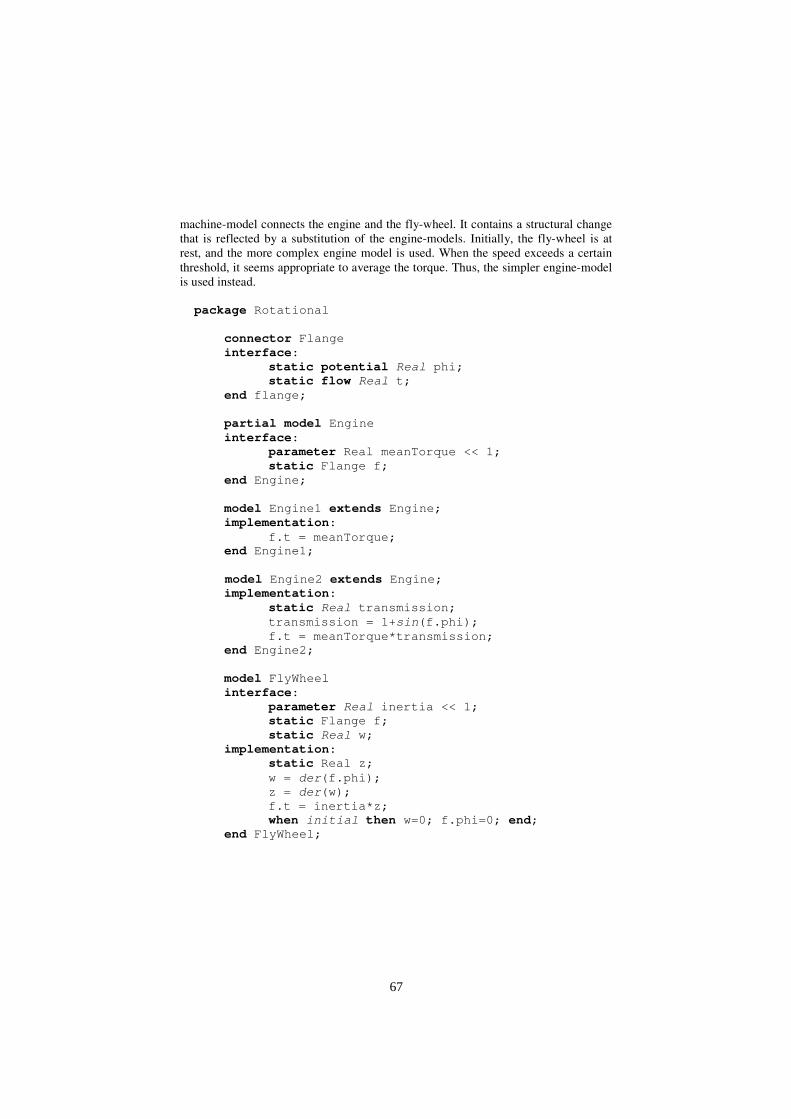
machine-model connects the engine and the fly-wheel. It contains a structural change

that is reflected by a substitution of the engine-models. Initially, the fly-wheel is at

rest, and the more complex engine model is used. When the speed exceeds a certain

threshold, it seems appropriate to average the torque. Thus, the simpler engine-model

is used instead.

package Rotational

connector Flange

interface:

static potential Real phi;

static flow Real t;

end flange;

partial model Engine

interface:

parameter Real meanTorque << 1;

static Flange f;

end Engine;

model Engine1 extends Engine;

implementation:

f.t = meanTorque;

end Engine1;

model Engine2 extends Engine;

implementation:

static Real transmission;

transmission = 1+sin(f.phi);

f.t = meanTorque*transmission;

end Engine2;

model FlyWheel

interface:

parameter Real inertia << 1;

static Flange f;

static Real w;

implementation:

static Real z;

w = der(f.phi);

z = der(w);

f.t = inertia*z;

when initial then w=0; f.phi=0; end;

end FlyWheel;

67

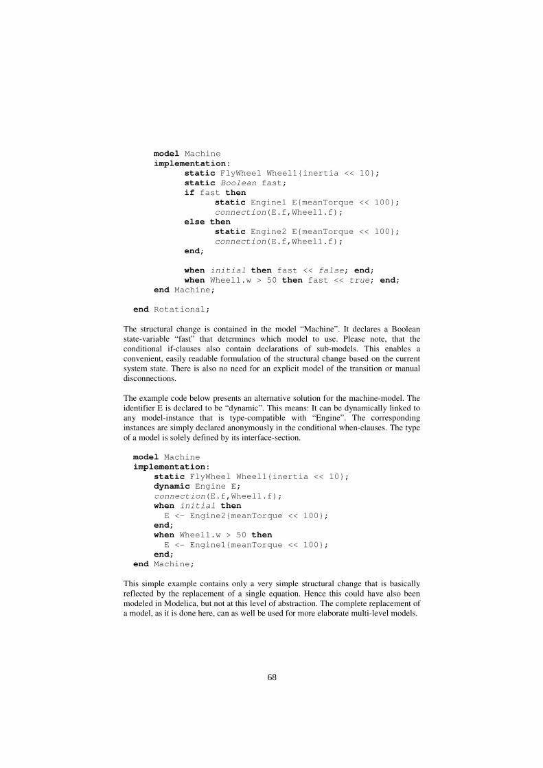
model Machine

implementation:

static FlyWheel Wheel1inertia << 10;

static Boolean fast;

if fast then

static Engine1 EmeanTorque << 100;

connection(E.f,Wheel1.f);

else then

static Engine2 EmeanTorque << 100;

connection(E.f,Wheel1.f);

end;

when initial then fast << false; end;

when Wheel1.w > 50 then fast << true; end;

end Machine;

end Rotational;

The structural change is contained in the model “Machine”. It declares a Boolean

state-variable “fast” that determines which model to use. Please note, that the

conditional if-clauses also contain declarations of sub-models. This enables a

convenient, easily readable formulation of the structural change based on the current

system state. There is also no need for an explicit model of the transition or manual

disconnections.

The example code below presents an alternative solution for the machine-model. The

identifier E is declared to be “dynamic”. This means: It can be dynamically linked to

any model-instance that is type-compatible with “Engine”. The corresponding

instances are simply declared anonymously in the conditional when-clauses. The type

of a model is solely defined by its interface-section.

model Machine

implementation:

static FlyWheel Wheel1inertia << 10;

dynamic Engine E;

connection(E.f,Wheel1.f);

when initial then

E <- Engine2meanTorque << 100;

end;

when Wheel1.w > 50 then

E <- Engine1meanTorque << 100;

end;

end Machine;

This simple example contains only a very simple structural change that is basically

reflected by the replacement of a single equation. Hence this could have also been

modeled in Modelica, but not at this level of abstraction. The complete replacement of

a model, as it is done here, can as well be used for more elaborate multi-level models.

68

4 Implementation and Ongoing Development

A first version of the language definition of Sol has been written down in the form of

an internal report. It forms the fundamentals for a corresponding implementation that

is currently under development. This implementation will be represented by an

interpreter that parses the model-file, instantiates a selected model and starts

simulation. In addition to its main task, the interpreter will provide various tools for

the analysis of the object-hierarchy, type-structure, etc.

Whereas the pair of a compiler and a simulator is the preferred choice for high-end

simulation tasks, an interpreter is an appropriate tool for research work on language

design. The development process becomes much easier, faster and more flexible.

Hence the development of the interpreter can proceed in parallel with a further

refinement of the language. Also, new debugging techniques will be needed that can

be better provided by an interpreter, since all necessary meta-information is available.

Of course, any interpreter (even if it is well written) suffers from a certain

computational overhead that may prevent its usage for highly demanding simulation

applications. Hence an important aspect will be to sketch the development of a

corresponding compiler.

4.1 Future goals

Sol is a language primarily conceived for research purposes. We want to explore the

full power of a declarative modeling approach and how it can handle potential, future

problem fields. Some of our goals and motivations are similar to [6], although we are

coming from a different direction. The implementation of Sol will be a small and

open project that should enable other researchers to test and validate their ideas with a

moderate effort. The longer term goal of our research is to significantly extend

Modelica’s expressiveness and range of application. Furthermore, the Sol-project

gives us a development-platform for technical solutions that concerns the handling of

structurally changing equation systems. This includes solutions for dynamic

recausalization or the dynamic handling of structural singularities.

It is not our target to immediately change the Modelica standard or to establish an

alternative modeling language. Our scientific work is intended to merely offer

suggestions and guidance for future development. This will primarily benefit the

future development of Modelica, but our results may also prove useful to other

modeling communities and researchers.

5. Conclusion

The development of a new modeling language should be a well considered step, since

it incorporates a lot of effort. This does not only concern the developers of the

language and the corresponding software, it includes as well the potential modelers

69

and users that are expected to get themselves acquainted with the new methodology.

However, the continuous progress of modeling technology generates a new set of

demands. This makes such a step finally inevitable.

In this workshop-paper, we offered a first glance of Sol, our new modeling language.

Sol has been designed to enable the modeling of variable-structure systems using an

equation-based framework. While its development is currently still at the beginning,

we expect to make significant progress in the near future. In the longer term, we hope

that our research will benefit Modelica’s future development.

References

1. Broman, D., Fritzson, P., Furic, S.: Types in the Modelica Language. In: Proceedings of the

Fifth International Modelica Conference, Vienna, Austria (2006) Vol. 1, 303-315

2. Cellier, F.E., Krebs, M.: Analysis and Simulation of Variable Structure Systems Using Bond

Graphs and Inline Integration. In: Proc. ICBGM’07, 8th SCS Intl. Conf. on Bond Graph

Modeling and Simulation, San Diego, CA, (2007) 29-34.

3. Elmqvist, H., Otter, M., Díaz López, D.: Collision Handling for the Modelica MultiBody

Library. In: Proc. 4th International Modelica Conference, Hamburg, Germany (2006) 45-53

4. Höpler, R., Otter, M.: A Versatile C++ Toolbox for Model Based, Real Time Control

Systems of Robotic Manipulators. In: Proc. of 2001 IEEE/RSJ International Conference on

Intelligent Robots and Systems, Maui, USA, (2001) 2208-2214

5. Otter, M., Elmqvist, H., Mattsson, S.E.: Hybrid Modeling in Modelica Based on the

Synchronous Data Flow Principle. In: Proc. IEEE International Symposium on Computer

Aided Control System Design, Hawaii. (1999) 151-157

6. Nilsson, H., Peterson J., Hudak, P.: Functional Hybrid Modeling. In: Proceedings of the 5th

International Workshop on Practical Aspects of Declarative Languages, New Orleans, LA

(2003) 376—390

7. Nytsch-Geusen, C. et. al.: Advanced modeling and simulation techniques in MOSILAB: A

system development case study. In: Proceedings of the Fifth International Modelica

Conference, Vienna, Austria (2006) Vol. 1, 63-71

8. Zimmer, D., Cellier, F.E., The Modelica Multi-bond Graph Library. In: Proc. 5th Intl.

Modelica Conference, Vienna, Austria (2006) Vol. 2, 559-568

70

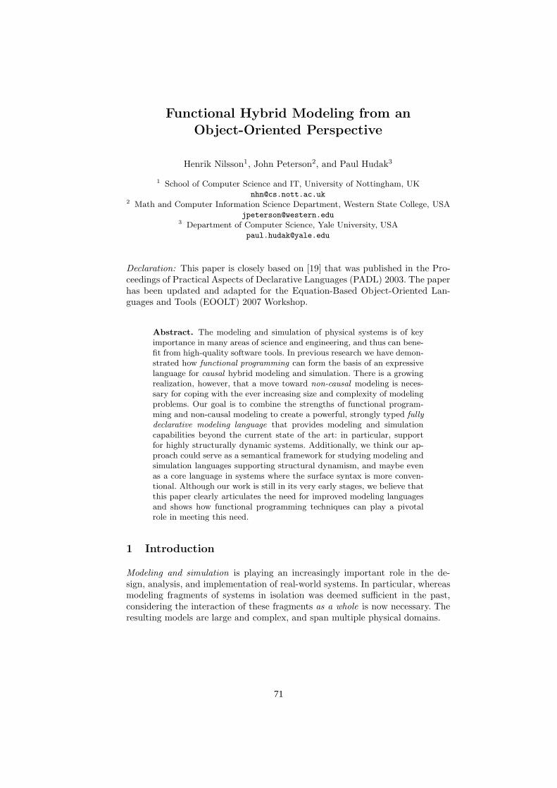
Functional Hybrid Modeling from an

Object-Oriented Perspective

Henrik Nilsson1, John Peterson2, and Paul Hudak3

1 School of Computer Science and IT, University of Nottingham, UKnhn@cs.nott.ac.uk

2 Math and Computer Information Science Department, Western State College, USAjpeterson@western.edu

3 Department of Computer Science, Yale University, USApaul.hudak@yale.edu

Declaration: This paper is closely based on [19] that was published in the Pro-ceedings of Practical Aspects of Declarative Languages (PADL) 2003. The paperhas been updated and adapted for the Equation-Based Object-Oriented Lan-guages and Tools (EOOLT) 2007 Workshop.

Abstract. The modeling and simulation of physical systems is of keyimportance in many areas of science and engineering, and thus can bene-fit from high-quality software tools. In previous research we have demon-strated how functional programming can form the basis of an expressivelanguage for causal hybrid modeling and simulation. There is a growingrealization, however, that a move toward non-causal modeling is neces-sary for coping with the ever increasing size and complexity of modelingproblems. Our goal is to combine the strengths of functional program-ming and non-causal modeling to create a powerful, strongly typed fullydeclarative modeling language that provides modeling and simulationcapabilities beyond the current state of the art: in particular, supportfor highly structurally dynamic systems. Additionally, we think our ap-proach could serve as a semantical framework for studying modeling andsimulation languages supporting structural dynamism, and maybe evenas a core language in systems where the surface syntax is more conven-tional. Although our work is still in its very early stages, we believe thatthis paper clearly articulates the need for improved modeling languagesand shows how functional programming techniques can play a pivotalrole in meeting this need.

1 Introduction

Modeling and simulation is playing an increasingly important role in the de-sign, analysis, and implementation of real-world systems. In particular, whereasmodeling fragments of systems in isolation was deemed sufficient in the past,considering the interaction of these fragments as a whole is now necessary. Theresulting models are large and complex, and span multiple physical domains.

71

Furthermore, these models are almost invariably hybrid : they exhibit bothcontinuous-time and discrete-time behaviors. In fact, the very structure of themodeled system changes over time. Such models are known as structurally dy-

namic. In general, the total number of structural configurations, or modes, canbe enormous, or even unbounded. We refer to systems whose number of modescannot be practically predetermined as highly structurally dynamic. While sup-porting structural dynamism is hard, supporting highly structurally dynamicsystems is even harder as this necessitates comprehensive and flexible solutionsof a number of important subproblems: see Sect. 5.

There are two broad language categories of modeling and simulation lan-guages. Causal (or block-oriented) languages are most popular; languages suchas Simulink and Ptolemy II [13] represent this style of modeling. In causal mod-eling, the equations that represent the physics of the system must be writtenso that the direction of signal flow, the causality, is explicit. The second, butless populated, class of language is non-causal, where the model focuses on theinterconnection of the components of the system being modeled, from whichcausality is then inferred. Such languages often support an object-oriented ap-proach to modeling. Examples include Dymola [5] and Modelica [15].

The main drawback of causal languages is the need to explicitly specify thecausality. This hampers modularity and reuse [2]. Non-causal languages addressthis problem by allowing the user to describe a model in a way which doesnot commit to any specific causality. The appropriate causality constraints arethen inferred using both symbolic and numerical methods depending on how themodel is being used. Unfortunately, current non-causal modeling languages tendto sacrifice generality when it comes to hybrid modeling: in particular, we arenot aware of any declarative non-causal modeling language that supports highlystructurally dynamic models, even if recent efforts like MOSILAB [20] and Sol[28] are important steps in that direction.

In previous research at Yale, we have developed a framework called Func-

tional Reactive Programming (FRP) [26], which is suited for causal hybrid mod-eling. This framework is embodied in a language called Yampa.4 as an extensionof Haskell. Yampa permits highly structurally dynamic hybrid systems to bedescribed clearly and concisely [18].5 In addition, because the full power of afunctional language is available, it exhibits a high degree of modularity, allowingreuse of components and design patterns. It also employs Haskell’s polymorphictype system to ensure that signals are connected consistently, even as the systemtopology changes. The semantic foundations of Yampa are well defined and un-derstood, making models expressed using Yampa suited for formal manipulationand reasoning. Yampa and its predecessors have been used in robotics simula-tion and control as well as a number of related domains [23, 24]. It has evenbeen used for video games [4, 3]. We are currently investigating biological cellpopulation modeling, where Yampa’s support for highly structurally dynamic

4 See http://haskell.org/yampa.5 However, at present, Yampa lacks integration with sophisticated numerical solvers,

and its applicability for serious simulation work is thus limited

72

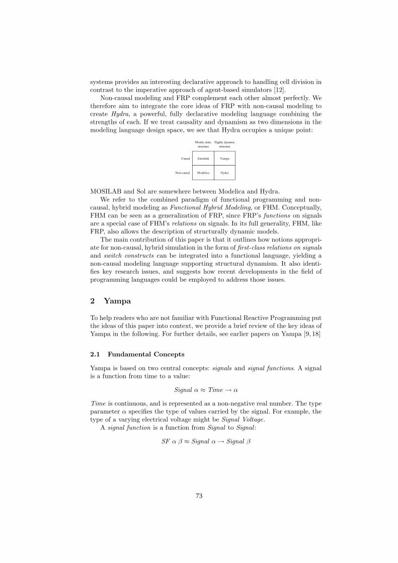
systems provides an interesting declarative approach to handling cell division incontrast to the imperative approach of agent-based simulators [12].

Non-causal modeling and FRP complement each other almost perfectly. Wetherefore aim to integrate the core ideas of FRP with non-causal modeling tocreate Hydra, a powerful, fully declarative modeling language combining thestrengths of each. If we treat causality and dynamism as two dimensions in themodeling language design space, we see that Hydra occupies a unique point:

MOSILAB and Sol are somewhere between Modelica and Hydra.We refer to the combined paradigm of functional programming and non-

causal, hybrid modeling as Functional Hybrid Modeling, or FHM. Conceptually,FHM can be seen as a generalization of FRP, since FRP’s functions on signalsare a special case of FHM’s relations on signals. In its full generality, FHM, likeFRP, also allows the description of structurally dynamic models.

The main contribution of this paper is that it outlines how notions appropri-ate for non-causal, hybrid simulation in the form of first-class relations on signals

and switch constructs can be integrated into a functional language, yielding anon-causal modeling language supporting structural dynamism. It also identi-fies key research issues, and suggests how recent developments in the field ofprogramming languages could be employed to address those issues.

2 Yampa

To help readers who are not familiar with Functional Reactive Programming putthe ideas of this paper into context, we provide a brief review of the key ideas ofYampa in the following. For further details, see earlier papers on Yampa [9, 18]

2.1 Fundamental Concepts

Yampa is based on two central concepts: signals and signal functions. A signalis a function from time to a value:

Signal α ≈ Time → α

Time is continuous, and is represented as a non-negative real number. The typeparameter α specifies the type of values carried by the signal. For example, thetype of a varying electrical voltage might be Signal Voltage.

A signal function is a function from Signal to Signal :

SF α β ≈ Signal α→ Signal β

73

When a value of type SF α β is applied to an input signal of type Signal α,it produces an output signal of type Signal β. Signal functions are first class

entities in Yampa. Signals, however, are not: they only exist indirectly throughthe notion of signal function. In general, the output of a signal function at timet is uniquely determined by the input signal on the interval [0, t]. If a signalfunction is such that the output at time t only depends on the input at the verysame time instant t, it is called stateless. Otherwise it is stateful.

2.2 Composing Signal Functions

(a) arr f (b) f ≫ g (c) f &&& g (d) loop f

Fig. 1: Basic signal function combinators.

Programming in Yampa consists of defining signal functions compositionallyusing Yampa’s library of primitive signal functions and a set of combinators.Yampa’s signal functions are an instance of the arrow framework proposed byHughes [10]. Three combinators from that framework are arr , which lifts anordinary function to a stateless signal function, and the two signal functioncomposition combinators ≪ and &&& :

arr :: (a → b)→ SF a b

(≪) :: SF b c → SF a b → SF a c

( &&& ) :: SF a b → SF a c → SF a (b, c)

We can think of signals and signal functions using a simple flow chart anal-ogy. Boxes represent signal functions, with one signal flowing in to the box’sinput port and another signal flowing out of the box’s output port. Figure 1illustrates some of the central arrow combinators using this analogy. The simi-larity to a block-oriented modeling language like Simulink is hopefully clear. Themain difference is that the notion of composing blocks into larger blocks has beenformalized through a handful of composition combinators, which is helpful froma semantical perspective, in contrast to the more unstructured approach of con-necting outputs to inputs in an arbitrary fashion.

2.3 Arrow Syntax

While the arrow framework provides a useful semantical structure, it is notconvenient for expressing large networks. It is much easier to simply connectwhatever needs to be connected Simulink style, e.g. by naming nodes and then

74

explicitly stating the connection topology. Fortunately, it is easy to provide alayer of syntax that allows this, and then translate this into a network descriptionin terms of the core arrow combinators. Paterson’s arrow notation [22] doesexactly that. An expression denoting a signal function has the form:

proc pat → do

pat1 ← sfexp1−≺ exp1

pat2 ← sfexp2−≺ exp2

. . .pat

n← sfexp

n−≺ exp

n

returnA−≺ exp

The keyword proc is analogous to the λ in λ-expressions, pat and pati

arepatterns binding signal variables pointwise by matching on instantaneous signalvalues, exp and exp

iare expressions defining instantaneous signal values, and

sfexpiare expressions denoting signal functions. The idea is that the signal being

defined pointwise by each expi

is fed into the corresponding signal functionsfexp

i, whose output is bound pointwise in pat

i. The overall input to the signal

function denoted by the proc-expression is bound by pat , and its output signalis defined by the expression exp. The signal variables bound in the patterns mayoccur in the signal value expressions, but not in the signal function expressionssfexp

i). An optional keyword rec, applied to a group of definitions, permits

signal variables to occur in expressions that textually precede the definition ofthe variable, allowing recursive definitions (feedback loops).

For a concrete example, consider the following:

sf = proc (a, b)→ do

(c1 , c2 )← sf1 &&& sf2−≺ a

d ← sf3 ≪ sf4−≺ (c1 , b)rec

e ← sf5−≺ (c2 , d , e)returnA−≺ (d , e)

Note the use of the tuple pattern for splitting sf ’s input into two “named signals”,a and b. Also note the use of tuple expressions and patterns for pairing andsplitting signals in the body of the definition; for example, for splitting theoutput from sf1 &&& sf2 . Also note how the arrow notation may be freely mixedwith the use of basic arrow combinators.

2.4 Events

While some aspects of a program are naturally modeled as continuous signals,other aspects are more naturally modeled as discrete events. To this end, Yampaintroduces the Event type, isomorphic to Haskell’s Maybe type:

data Event a = NoEvent | Event a

75

The instantaneous value of signal of type Event T for some type T is eitherNoEvent or Event x for some value x of type T , thus mimicking a discrete-timesignal that is only defined at discrete points in time.

2.5 Switching

The structure of a Yampa system may evolve over time. These structural changesare known as mode switches. This is accomplished through a family of switching

primitives that use events to trigger changes in the connectivity of a system. Thesimplest such primitive is switch:

switch :: SF a (b,Event c)→ (c → SF a b)→ SF a b

The switch combinator switches from one subordinate signal function into an-other when a switching event occurs. Its first argument is the signal functionthat initially is active. It outputs a pair of signals. The first defines the overalloutput while the initial signal function is active. The second signal carries theevent that will cause the switch to take place. Once the switching event occurs,switch applies its second argument to the value of the event and switches intothe resulting signal function.

Thus, note that the second argument of switch is a function of type c →SF a b, that, when given the value of type c carried by the event, dynamically

computes a new signal function to switch into. Using a Simulink analogy, switch

in principle rips out a block, and then dynamically instantiates a parameterizedblock as a replacement. The design of switch thus exploits the fact that signalfunctions (“blocks”) are first class entities in Yampa.

Yampa also includes parallel switching constructs that maintain dynamic

collections of signal functions connected in parallel [18]. Signal functions can beadded to or removed from such a collection at runtime in response to events,while preserving any internal state of all other signal functions in the collection;see Fig. 2. The first class status of signal functions in combination with switchingover dynamic collections of signal functions makes Yampa an unusually flexiblelanguage for describing hybrid systems. For example, this makes it possible tohandle systems where the number of modeled entities varies over time, like cellpopulation models as mentioned earlier (Sect. 1).

Fig. 2: System of interconnected signal functions with varying structure

76

l

φ

m

u

mg

(a) Pendulum

model BreakingPendulum

parameter Real m=1, g=9.81, L=0.5;

parameter Boolean Broken;

input Real u;

Real pos[2], vel[2];

Real phi(start=PI/4), phid;

equation

vel = der(pos);

if not Broken then

// Equations of pendulum.

pos = L*sin(phi), -L*cos(phi);phid = der(phi);

m*L*L*der(phid) + m*g*L*sin(phi) = u;

else

// Equations of free-flying mass.

m*der(vel) = m*0, -g;end if;

end BreakingPendulum;

(b) Modelica model

Fig. 3: A pendulum, subject to externally applied torque and gravity.

3 Non-Causal and Hybrid Modeling

While the simulation of pure continuous systems is relatively well understood,hybrid systems pose a number of unique challenges [16, 1]. Problems includehandling a large number of modes, event detection, and consistent initializationof state variables. The integration of hybrid modeling with non-causal modelingraises further problems. Indeed, current non-causal modeling languages are quitelimited in their ability to express hybrid systems. Many of the limitations arerelated to the symbolic and numerical methods that must be used in the non-causal approach. But another important reason is that most such systems insiston performing all symbolic manipulations before simulation begins [16]. Avoidingthese limitations is an important part of our approach, see Sec. 5.

Since Modelica is representative of state-of-the-art, non-causal, hybrid model-ing languages, we illustrate the limitations of present languages with an examplefrom the Modelica documentation [14, pp. 31–33]. The system is a pendulum inthe form of a mass m at the end of a rigid, mass-less rod, subject to gravitymg and an externally applied torque u at the point of suspension; see Fig. 3(a).Additionally, the rod could break at some point, causing the mass to fall freely.

Figure 3(b) shows a Modelica model of this system that, on the surface,looks like it achieves the desired result. Note that it has two modes, described byconditional equations. In the non-broken mode, the position pos and velocity vel

of the mass are calculated from the state variables phi and phid. In the brokenmode, pos and vel become the new state variables. This implies that stateinformation has to be transferred between the non-broken and broken mode.Furthermore, the causality of the system is different in the two modes. When

77

non-broken, the equation relating vel and pos is used to compute vel from pos.When broken, the situation is reversed.

These facts make simulation hard. Modelica attempts to simplify matters byavoiding too radical structural changes. To that end, Modelica either requiresthe condition for selecting between two sets of equation to be a parameter, andthus unchanging during simulation, or else that the number of equations in eachset are the same. In this case, as the number of equations is not the same, Brokenhas to be declared a parameter. Therefore the model above does not really solvethe hybrid simulation problem at all! In order to actually model a pendulumthat dynamically breaks at some point in time, the model must be expressed insome other way. The Modelica documentation suggests a causal, block-orientedformulation with explicit state transfer. Unsurprisingly, the result is considerablymore verbose, nullifying the advantage of working in a non-causal language.

Moreover, even if Broken were allowed to be a dynamic variable, a funda-mental problem would remain: once the pendulum has broken, it cannot becomewhole again. Modelica provides no way to declaratively express the irreversibil-

ity of this structural change. The best that can be done is to capture this factindirectly through a state machine model that control the value of Broken.

4 Integrating Functional Programming and Non-Causal

Modeling

In the preceding sections we discussed the advantages of non-causal modeling andthe importance of hybrid modeling. We also pointed out serious shortcomingsin current modeling languages with respect to these features. In this section, wedescribe a new way to combine non-causal and hybrid modeling techniques thataddresses these issues. Inspired by FRP and Yampa, the two key ideas are togive first-class status to relations on signals and to provide constructs for discreteswitching between relations. The result is Hydra, a functional hybrid modelinglanguage capable of representing structurally dynamic systems.

While we, based on our experience of Yampa, believe that a language like Hy-dra would be a very expressive and powerful modeling and simulation languagein its own right, we would like to emphasize that we also think our approachcould serve as a valuable semantical framework for general study of modelingand simulation languages that supports structural dynamism, and maybe evenas a core language in systems where the surface syntax is more conventional.Thus, what is important in the following is not the syntax (which is tentativeand likely lacking in many ways), but the underlying principles.

4.1 First-Class Signal Relations

A natural mathematical description of a continuous signal function is that of anODE in explicit form. A function is just a special case of the more general conceptof a relation. While functions usually are given a causal interpretation, relationsare inherently non-causal. Differential Algebraic Equations (DAEs), which are

78

at the heart of non-causal modeling, express dependences among signals withoutimposing a causality on the signals in the relation. Thus it is natural to viewthe meaning of a DAE as a non-causal signal relation, just as the meaning ofan ODE in explicit form can be seen as a causal signal function. Since signalfunctions and signal relations are closely connected, this view offers a clean wayof integrating non-causal modeling into an Yampa-like setting.

In the following, first-class signal relations are made concrete by proposing a(tentative) system for integrating them into a polymorphically typed functionallanguage. Signal functions are also useful, but since they are just relations withexplicit causality, we need not consider them in detail in the following.

Similarly to the signal function type SF of Yampa (Sect. 2.1), we introducethe type SR α for a relation on a signal of type Signal α. Specific relations usea more refined type; e.g., for the derivative relation der we have the typing:

der :: SR (Real , Real)

Since a signal carrying pairs is isomorphic to a pair of signals, we can understandder as a binary relation on two real-valued signals.

Next we need a notation for defining relations. Inspired by the arrow notation(Sect. 2.3), we introduce the following to denote a signal relation:

sigrel pattern where equations

The pattern introduces signal variables that at each point in time are bound tothe instantaneous value of the corresponding signal. Given p :: t, we have:

sigrel p where . . . :: SR t

Consequently, the equations express relationships between instantaneous sig-nal values. This resembles the standard notation for differential equations inmathematics. For example, consider x′ = f(y), which means that the instanta-neous value of the derivative of (the signal) x at every time instant is equal tothe value obtained by applying the function f to the instantaneous value of y.

We introduce two styles of equations:

e1 = e2

sr ⋄ e3

where ei are expressions (possibly introducing new signal variables), and sr isan expression denoting a signal relation. We require equations to be well-typed.Given ei :: ti, this is the case iff t1 = t2 and sr :: SR t3.

The first kind of equation requires the values of the two expressions to beequal at all points in time. For example:

f(x) = g(y)

where f and g are functions.The second kind allows an arbitrary relation to be used to enforce a relation-

ship between signals. The symbol ⋄ can be thought of as relation application;

79

the result is a constraint which must hold at all times. The first kind of equationis just a special case of the second in that it can be seen as the application ofthe identity relation.

For another example, consider a differential equation like x′ = f(x, y). Usingour notation, this equation could be written:

der ⋄ (x, f(x, y))

where der is the relation relating a signal to its derivative. For convenience, anotation closer to the mathematical tradition should be supported as well:

der(x) = f(x, y)

The meaning is exactly as in the first version.

i

+

R1 R2

C L

G

uL

i2

uR2

uC

i1

R1u

uin

Fig. 4: A simple electrical circuit.

We illustrate our language by modeling the electrical circuit in Fig. 4.1(adapted from [14]). The type Pin is a record type describing an electrical con-nection. It has fields v for voltage and i for current.6

twoPin :: SR (Pin , Pin, Voltage)twoPin = sigrel (p, n, u) where

u = p.v − n.vp.i + n.i = 0

resistor :: Resistance → SR (Pin , Pin)resistor(r) = sigrel (p, n) where

twoPin ⋄ (p, n, u)r · p.i = u

6 The name Pin is perhaps a bit misleading since it just represents a pair of physicalquantities, not a physical “pin component”; i.e., Pin is the type of signal variablesrather than signal relations.

80

inductor :: Inductance → SR (Pin , Pin)inductor(l) = sigrel (p, n) where

twoPin ⋄ (p, n, u)l · der(p.i) = u

capacitor :: Capacitance → SR (Pin , Pin)capacitor (c) = sigrel (p, n) where

twoPin ⋄ (p, n, u)c · der(u) = p.i

As in Modelica, the resistor, inductor and capacitor models are defined as exten-sions of the twoPin model. However, we accomplish this directly with functionalabstraction rather than the Modelica class concept. Note how parameterizedmodels are defined through functions returning relations. Since the parametersare normal function arguments, not signal variables, their values remain un-changed throughout the lifetime of the returned relations.7

To assemble these components into the full model, we adopt a Modelica-like connect-notation as a convenient abbreviation for connection equations.This is syntactic sugar which is expanded to proper connection equations, i.e.equality constraints or sum-to-zero equations depending on what kind of physicalquantity is being connected. We assume that a voltage source model vSourceAC

and a ground model ground are available in addition to the component modelsdefined above. Moreover, we are only interested in the total current through thecircuit, and, as there are no inputs, the model thus becomes a unary relation:

simpleCircuit :: SR Current

simpleCircuit = sigrel i where

resistor(1000) ⋄ (r1p, r1n)resistor(2200) ⋄ (r2p, r2n)capacitor (0.00047) ⋄ (cp, cn)inductor(0.01) ⋄ (lp, ln)vSourceAC (12) ⋄ (acp, acn)ground ⋄ gp

connect acp, r1p, r2pconnect r1n, cpconnect r2n, lpconnect acn, cn, ln, gpi = r1p.i + r2p.i

4.2 Modeling Systems with Dynamic Structure

In order to describe structurally dynamic systems we need to represent an evolv-ing structure. To this end, we introduce two Yampa-inspired switching con-structs: the recurring switch and the progressing switch. The recurring switch

7 Compare to Modelica’s parameter-variables mentioned in Sect. 3.

81

allows repeated switching between equation groups. In contrast, the progressingswitch expresses that one group of equations first is in force, and then, once theswitching condition has been fulfilled, another group, thus irreversibly progress-ing to a new structural configuration. For either sort of switching, difficult issuessuch as state transfer and proper initialization have to be considered.

We revisit the breaking pendulum example from Sect. 3 to illustrate theseswitching constructs. To deal with initialization and state transfer, we introducespecial initialization equations that are only active at the time of switching, thatis, during events, and we allow such equations to refer to the values of signalvariables just prior to the event through a special pre-construct devised for thatpurpose. The initialization equations describe the initial conditions of the DAEafter a switch. Mathematically, these equations must yield an initial value forevery state variable in the new continuous equations. It is important that eachbranch of a switch can be associated with its own initialization equations, sinceeach such branch may introduce its proper set of state variables. Initializationequations typically state continuity assumptions, like pos and vel below.

First, consider a direct transliteration of the equation part of the Modelicamodel using a recurring switch. The necessary initialization equations have alsobeen added:

vel = der(pos)switch broken

when False then

init phi = pi/4init phid = 0pos = l · sin (phi),−l · cos (phi)phid = der(phi)m · l · l · der(phid ) + m · g · l · sin (phi) = u

when True then

init vel = pre(vel)init pos = pre(pos)m · der(vel) = m · 0,−g

A recurring switch has one or more when-branches. The idea is that the equa-tions in a when-branch are in force whenever the pattern after when (whichmay bind variables) matches the value of the expression after switch. Thus,whenever that value changes, we have an event and a switch occurs (this issimilar to case in a functional language).

To express the fact that the pendulum cannot become whole once it hasbroken, we refine the model by changing to a progressing switch:

vel = der(pos)switch broken

first

. . .once True then

. . .

82

A progressing switch has one first-branch and one or more once-branches.Initially, the equations in the first-branch are in force, but as soon as the valueof the expression after switch matches one of the once-patterns, a switch occursto the equations in the corresponding branch, after which no further switchingoccurs (for that particular instance of the switch).

By combining recursively-defined relations and progressing switches, it ispossible to express very general sequences of structural changes over time, fromsimple mode transitions to making and breaking of connections between objects.A simple example of a recursively defined relation parameterized on a discretestate variable n is shown below. Initially, the relation behaves according to theequations in the first-branch, which may depend on n. Whenever the switchingcondition is fulfilled, the relation switches to a new instance of itself with theparameter n increased by one. In functional parlance, this is a form of tail call.

sysWithCntr :: Int → SR (Real , Real)sysWithCntr(n) = sigrel (x, y) where

switch . . .first

. . .once . . . then

sysWithCntr(n + 1) ⋄ (x, y)

As explained in Sect. 2.5, Yampa supports even more radical structural changes,including dynamic addition and deletion of objects. Our goal is to carry over asmuch as possible of that functionality to Hydra.

5 Implementation Issues

There are a number of challenges that must be addressed in an implementationof a language like Hydra. The primary issues are ensuring model correctness,simulation in the presence of dynamic mode changes, and mode initialization.

It is critical that dynamic changes in the model should should not weaken thestatic checking of the model, i.e. we want to ensure compositional correctness.A Haskell-like polymorphic type system, as in Yampa, ensures that the systemintegrity is preserved. In addition we would like to find at least necessary con-ditions for statically ensuring that causality analysis can always be carried out,that the equations at least could have a solution, and so on, regardless of howrelations are composed dynamically. An example of a necessary but not sufficientcondition is that the number of equations and number of variables agree, andthat each variable can be paired with one equation. Since it will be necessaryto keep track of the balance between equations and variables across relationboundaries, it is natural to integrate this aspect into the type system. Similarconsiderations apply to the number of initialization equations and continuousstate variables. Recent work on dependent types is relevant here [27]. We alsoaim at extending the type system to handle physical dimensions [11].

83

In a highly structurally dynamic language, it is impossible to identify allpossible operating modes and then factor them out as separate systems. Modesthus have to be generated dynamically during simulation as follows. Whenever aswitch occurs, a new, global, “flattened” DAE has to be generated. The DAE isobtained by first carrying out the necessary discrete processing, which amountsto standard functional evaluation, including evaluation of the relational expres-

sions in the equations that are to be active after the switch. The evaluation ofrelational expression is what creates new instances of relations, and carrying outthe instantiation dynamically when switching occurs is what enables modelingof highly structurally dynamic systems. Once the new flattened DAE has beengenerated, it is subjected to causality analysis and other symbolic manipula-tions in preparation for simulation using suitable numerical methods [21, 6, 7].The result is causal simulation code.

The hybrid bond graph simulator HyBrSim has demonstrated the feasibilityof this dynamic approach, and that it indeed allows some difficult cases to behandled [17]. However, HyBrSim is an interpreted system. Simulation is thusslowed down both by occasional symbolic processing and by the interpretiveoverhead. To avoid interpretive overhead, we intend to leverage recent workon run-time code generation, such as ‘C [8] or Cyclone [25]. We will need toadapt the sophisticated mathematical techniques used in existing non-causalmodeling languages [21, 6, 7] to this setting. In part, it may be possible to dothis systematically by staging the existing algorithms in a language like Cyclone.

The initial conditions of the (new) differential equations must be determinedon transitions from one mode to another. However, arriving at consistent initialconditions is, in general, hard. Some state variables in the continuous part ofthe system may exhibit discontinuities at the time of switching while others willnot: simply preserving the old value is not always the right solution. Structuralchanges could change the set of state variables, and the relationship between thenew and old states may be difficult to determine. One approach is to requirethe modeler to provide a function that maps the old state to the new one foreach possible mode transition [1]. However, the declarative formulation of non-causal models means that the simulator sometimes has a choice regarding whichcontinuous variables should be treated as state variables. Requiring the user toprovide a state mapping function is therefore not always reasonable.

A key to the success of HyBrSim is that bond graphs are based on physicalnotions such as energy and energy exchange, which are subject to continuity andconservation principles. We intend to generalize this idea by exploring the use ofdeclarations for stating such principles, along the lines illustrated in Sec. 4.2. Itmay also be possible to infer continuity and conservation constraints automati-cally based on physical dimension types.

6 Related Work

There has been substantial interest in supporting structural dynamism withinthe non-causal modeling community recently. The most advanced effort at present

84

is probably MOSILAB [20]. Similarly to what is proposed here, MOSILAB sup-ports dynamic addition and deletion of behavioral objects. The switching is con-trolled through a form statecharts. A modern, sophisticated DAE solver, withsupport for computing consistent initial conditions, is used.

However, the statechart approach implies an explicit enumeration of themodes, and even if the number of modes could be large due to combinatorial ef-fects, this rules out a Yampa-style, truly dynamic number of simulation objects,which is the ultimate goal of Hydra.

Another aspect of MOSILAB is the use of Python for various meta-modelingtasks, such as writing “experiment scripts”. We think that Hydra in itself, thanksto being a general-purpose functional language with first-class signal relationsand functions, should be expressive enough to mostly provide equivalent meta-modeling capabilities, all in a uniform, declarative setting, without resorting toexternal imperative languages.

Sol [28] is another effort to create a non-causal modeling and simulationlanguage supporting structural dynamism. It expressively avoids the statechartapproach to retain more of the declarative clarity of languages like Modelica. It isalso claimed that the Sol approach to dynamism scales better. A key aspect of theSol approach is the capability to dynamically determine model instances. Thisidea seems to be somewhat similar to the notion of first-class signal functionsand relations in Hydra. Like MOSILAB, Sol seems to stop short of the Hydragoal of supporting systems with a dynamic number of objects.

7 Conclusions

Hybrid modeling is a domain in which the techniques of declarative programminglanguages have the potential to greatly advance the state of the art. The model-ing community has traditionally been concerned more with the mathematics ofmodeling than language issues. As a result, present modeling languages do notscale in a number of ways, particularly in hybrid systems that undergo significantstructural changes. Hydra uses functional programming techniques to describedynamically changing systems in a way that preserves the non-causal structureof the system specification and allows arbitrary switching among modes, yieldingexpressive power beyond current non-causal modeling languages.

Although we have not completed an implementation of Hydra, this paperdemonstrates our basic design approach and maps out the design landscape. Weexpect that further research into the links between declarative languages andhybrid modeling will produce significant advances in this field.

Acknowledgments The authors would like to thank the anonymous EOOLTreviewers for many useful suggestions for adapting the paper to this venue.

References

1. Paul I. Barton and Cha Kun Lee. Modeling, simulation, sensitivity analysis, andoptimization of hybrid systems. Submitted to ACM Transactions on Modelling

85

and Computer Simulation: Special Issue on Multi-Paradigm Modeling, September2001.

2. Francois E. Cellier. Object-oriented modelling: Means for dealing with systemcomplexity. In Proceedings of the 15th Benelux Meeting on Systems and Control,Mierlo, The Netherlands, pages 53–64, 1996.

3. Mun Hon Cheong. Functional programming and 3D games. BEng thesis, Universityof New South Wales, Sydney, Australia, November 2005.

4. Antony Courtney, Henrik Nilsson, and John Peterson. The Yampa arcade. InProceedings of the 2003 ACM SIGPLAN Haskell Workshop (Haskell’03), pages7–18, Uppsala, Sweden, August 2003. ACM Press.

5. Hilding Elmqvist, Francois E. Cellier, and Martin Otter. Object-oriented modelingof hybrid systems. In Proceedings of ESS’93 European Simulation Symposium,pages xxxi–xli, Delft, The Netherlands, 1993.

6. Hilding Elmqvist and Martin Otter. Methods for tearing systems of equations inobject-oriented modeling. In Proceedings of ESM’94, European Simulation Multi-conference, pages 326–332, Barcelona, Spain, June 1994.

7. Hilding Elmqvist, Martin Otter, and Francois E. Cellier. Inline integration: A newmixed symbolic/numeric approach. In Proceedings of ESM’95, European Simula-tion Multiconference, pages xxiii–xxxiv, Prague, Czech Republic, June 1995.

8. Dawson R. Engler, Wilson C. Hsieh, and M. Frans Kaashoek. ‘C: A languagefor high-level, efficient, and machine-independent dynamic code generation. InProceedings of the 23rd ACM Symposium on Principles of Programming Languages(POPL’96), pages 131–144, January 1996.

9. Paul Hudak, Antony Courtney, Henrik Nilsson, and John Peterson. Arrows, robots,and functional reactive programming. In Johan Jeuring and Simon Peyton Jones,editors, Advanced Functional Programming, 4th International School 2002, volume2638 of Lecture Notes in Computer Science, pages 159–187. Springer-Verlag, 2003.

10. John Hughes. Generalising monads to arrows. Science of Computer Programming,37:67–111, May 2000.

11. Andrew Kennedy. Programming Languages and Dimensions. PhD thesis, Uni-versity of Cambridge, Computer Laboratory, April 1996. Published as TechnicalReport No. 391.

12. John King, Michael Lees, and Brian Logan. Agent-based and continuum modellingof populations of cells. Technical report, University of Nottingham, December 2006.

13. Edward A. Lee. Overview of the Ptolemy project. Technical memorandumUCB/ERLM01/11, Electronic Research Laboratory, University of California,Berkeley, March 2001.

14. The Modelica Association. Modelica – A Unified Object-Oriented Lan-guage for Physical Systems Modeling: Tutorial version 1.4, December 2000.http://www.modelica.org/documents/ModelicaTutorial14.pdf.

15. The Modelica Association. Modelica – A Unified Object-Oriented Language forPhysical Systems Modeling: Language Specification version 2.2, February 2005.http://www.modelica.org/documents/ModelicaSpec22.pdf.

16. Pieter J. Mosterman. An overview of hybrid simulation phenomena and theirsupport by simulation packages. In Fritz W. Vaadrager and Jan H. van Schuppen,editors, Hybrid Systems: Computation and Control ’99, number 1569 in LectureNotes in Computer Science, pages 165–177, 1999.

17. Pieter J. Mosterman, Gautam Biswas, and Martin Otter. Simulation of disconti-nuities in physical system models based on conservation principles. In Proceedingsof SCS Summer Conference 1998, pages 320–325, July 1998.

86

18. Henrik Nilsson, Antony Courtney, and John Peterson. Functional reactive pro-gramming, continued. In Proceedings of the 2002 ACM SIGPLAN Haskell Work-shop (Haskell’02), pages 51–64, Pittsburgh, Pennsylvania, USA, October 2002.ACM Press.

19. Henrik Nilsson, John Peterson, and Paul Hudak. Functional hybrid modeling.In Proceedings of PADL’03: 5th International Workshop on Practical Aspects ofDeclarative Languages, volume 2562 of Lecture Notes in Computer Science, pages376–390, New Orleans, Lousiana, USA, January 2003. Springer-Verlag.

20. Christoph Nytsch-Geusen et al. MOSILAB: Development of a Modelica basedgeneric simulation tool supporting model structural dynamics. In Proceedings of the4th International Modelica Conference, Hamburg, Germany, March 2005. ModelicaAssociation.

21. Constantinos C. Pantelides. The consistent initialization of differential-algebraicsystems. SIAM Journal on Scientific and Statistical Computing, 9(2):213–231,March 1988.

22. Ross Paterson. A new notation for arrows. In Proceedings of the 2001 ACMSIGPLAN International Conference on Functional Programming, pages 229–240,Firenze, Italy, September 2001.

23. John Peterson, Greg Hager, and Paul Hudak. A language for declarative roboticprogramming. In Proceedings of IEEE Conference on Robotics and Automation,May 1999.

24. John Peterson, Paul Hudak, Alastair Reid, and Greg Hager. FVision: A declar-ative language for visual tracking. In Proceedings of PADL’01: 3rd InternationalWorkshop on Practical Aspects of Declarative Languages, pages 304–321, January2001.

25. Frederick Smith, Dan Grossman, Greg Morrisett, Luke Hornof, and Trevor Jim.Compiling for run-time code generation. Submitted for publication to JFP SAIG.

26. Zhanyong Wan and Paul Hudak. Functional reactive programming from first prin-ciples. In Proceedings of PLDI’01: Symposium on Programming Language Designand Implementation, pages 242–252, June 2000.

27. Hongwei Xi and Frank Pfenning. Dependent types in practical programming. InProceedings of ACM SIGPLAN Symposium on Principles of Programming Lan-guages, pages 214–227, San Antonio, January 1999.

28. Dirk Zimmer. Enhancing Modelica towards variable structure systems. In Proceed-ings of 1st International Workshop on Equation-Based Object-Oriented Languagesand Tools (EOOLT 2007), Berlin, Germany, July 2007. LiU E-Press.

87

Important Characteristics of VHDL-AMS and Modelica with Respect to Model Exchange

Olaf Enge-Rosenblatt, Joachim Haase, Christoph Clauß

Fraunhofer Institute for Integrated Circuits, Design Automation Division, Zeunerstr. 38

D-01069 Dresden, Germany Olaf.Enge, Joachim.Haase, Christoph.Clauss @eas.iis.fraunhofer.de

Abstract. Modeling and simulation have been established as fundamental facilities in the development of analog and analog-digital systems. Essential advances have been achieved by the usage of behavioral modeling languages. These languages can be considered as a link between the technical problem and the mathematical model that can be evaluated by computational methods. The paper outlines the various possibilities that are offered by the language VHDL-AMS – standardized by the IEEE to describe analog and mixed-signal systems – and the language Modelica. The underlying modeling approaches are compared. Last but not least, the potential to transform models written in one language into models of the other language is discussed.

Keywords: VHDL-AMS, Modelica, model exchange

1 Introduction

A multitude of behavioral modeling languages has been developed during recent years [1, 2, 3, 4]. They provide among other things a link between the mathematical description of an object and a representation that can be used by a simulation engine. Currently it can not be expected that all languages are supported by all simulation tools. On the other hand, large efforts have been spent on developing model libraries. Possibilities and limitations of the transformation of models written in VHDL-AMS [1] and Modelica [2] are discussed in the paper.

VHDL-AMS is a behavioral modeling language that is an extension of VHDL for the analysis of analog and mixed-signal systems. The language is standardized by IEEE. VHDL was originally developed to describe and model digital electronic circuits. The analog and mixed signal extensions were partly based on the experiences with the program Spice [5]. This is a program to simulate Kirchhoffian networks. Spice-like simulation tools have been available for more than thirty years. The first implementations of tool-specific behavioral languages to describe the analog behavior include for instance MAST [6] which is one of the ancestors of VHDL-AMS.

Modelica is a modeling language that allows the specification of complex systems. Especially it is widely used to describe non-electrical systems. The description of analog systems is supported as well as discrete, hybrid, and concurrency modeling.

89

A very active community has developed many models and libraries during recent years.

From a general point of view, both languages have a lot of similarities. Modeling is primarily based on equations. A system description can be established by connecting subsystems in a hierarchical way. A system of equations that considers the restrictions of the unknowns with respect to the terminal behavior of the subsystems, the topology of the final system, and some augmentation sets (for example to describe initial conditions) are generated. Both languages support the modeling of time-continuous conservative systems (based on a network approach), non-conservative systems (described by signal-flow blocks), and time-discrete systems. Modeling of multidomain systems that consist of electrical and non-electrical components is possible.

The time-continuous part of a well-established analysis problem is described by a differential algebraic system of equations [7] of form

0)),('),(( =ttxtxF (1)

with nnn RRRRF →×× +: and nRRx →+:

The solution method is not defined by the language descriptions. The VHDL-AMS language reference manual [1] defines characteristic equations

that must be fulfilled by the solution. The structural set of these equations considers the Kirchhoff laws and represents the equality of quantities at the connection points of non-conservative ports. The explicit set is given by the simultaneous statements of the models. In the case of a conservative network, these equations describe the branch constitutive relations. Additional restrictions that must be considered in the initialization phase and at discontinuities are established by the augmentation set. It has to be considered during modeling that these equations must be fulfilled by a solution of the simulation problem [8]. A solvability check is done at the design unit level. Roughly spoken, the number of essential unknowns that are contributed by a model to the characteristic equations of the entire system must match the number of explicitly added model equations. In the case of VHDL-AMS simulators, the unknowns that fulfill the characteristic expressions are determined using a modified nodal analysis approach [9]. In this way, the dimension n of the system of form (1) that is solved by the simulator is reduced compared to the number of characteristic equations. The time-discrete part is solved by event-driven simulation approaches. Besides time domain simulation, small signal frequency and noise domain simulation are supported by VHDL-AMS. The language reference manual describes how to establish the characteristic expressions in these cases. They base on a linearization of (1) around the operating point.

A similar mechanism is used in Modelica. For each connection point of instances of an entire system connection equations contribute to the system (1). These equations correspond to the structural set in VHDL-AMS. The non-flow variables are set equal and the flow variables are summed to zero. The equations of each instance are included to build up (1). They represent the explicit set in VHDL-AMS. Additional requirements can be expressed to initialize unknowns in the initialization phase or to reinitialize values after discontinuities. This is similar to the augmentation set in VHDL-AMS. In contrast to VHDL-AMS, violations of these augmented equations

90

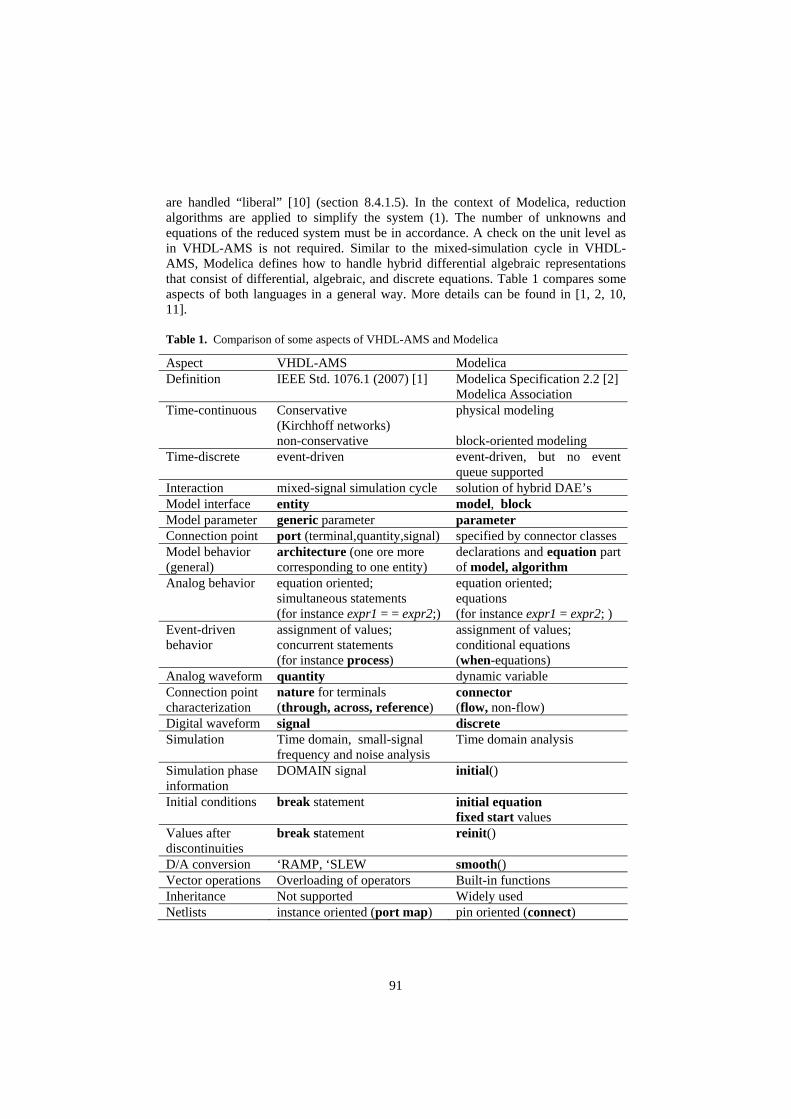
are handled “liberal” [10] (section 8.4.1.5). In the context of Modelica, reduction algorithms are applied to simplify the system (1). The number of unknowns and equations of the reduced system must be in accordance. A check on the unit level as in VHDL-AMS is not required. Similar to the mixed-simulation cycle in VHDL-AMS, Modelica defines how to handle hybrid differential algebraic representations that consist of differential, algebraic, and discrete equations. Table 1 compares some aspects of both languages in a general way. More details can be found in [1, 2, 10, 11].

Table 1. Comparison of some aspects of VHDL-AMS and Modelica

Aspect VHDL-AMS Modelica Definition IEEE Std. 1076.1 (2007) [1] Modelica Specification 2.2 [2]

Modelica Association Time-continuous Conservative

(Kirchhoff networks) non-conservative

physical modeling block-oriented modeling

Time-discrete event-driven event-driven, but no event queue supported

Interaction mixed-signal simulation cycle solution of hybrid DAE’s Model interface entity model, block Model parameter generic parameter parameter Connection point port (terminal,quantity,signal) specified by connector classes Model behavior (general)

architecture (one ore more corresponding to one entity)

declarations and equation part of model, algorithm

Analog behavior equation oriented; simultaneous statements (for instance expr1 = = expr2;)

equation oriented; equations (for instance expr1 = expr2; )

Event-driven behavior

assignment of values; concurrent statements (for instance process)

assignment of values; conditional equations (when-equations)

Analog waveform quantity dynamic variable Connection point characterization

nature for terminals (through, across, reference)

connector (flow, non-flow)

Digital waveform signal discrete Simulation Time domain, small-signal

frequency and noise analysis Time domain analysis

Simulation phase information

DOMAIN signal initial()

Initial conditions break statement initial equation fixed start values

Values after discontinuities

break statement reinit()

D/A conversion ‘RAMP, ‘SLEW smooth() Vector operations Overloading of operators Built-in functions Inheritance Not supported Widely used Netlists instance oriented (port map) pin oriented (connect)

91

The classes of problems that can be described with both languages seem to be very similar. Thus, it is obvious to check the possibilities to use models described in both languages together or to transform from one language into the other. In the following, aspects of the transformation of Modelica models into VHDL-AMS models are especially considered.

2 Modeling Approaches in VHDL-AMS and Modelica

Fig. 1. Terminal behavior of conservative (electrical) systems in Modelica and VHDL-AMS (examples)

A physical Modelica model describes the relation between pin flow and pin potential variables (see for example in Fig. 1 p.i and p.v resp.) by a set of equations. Additional variables can be introduced. Usually the number of equations equals the sum of the number of pins and additional variables. This is not strictly required but usually fulfilled. It is only required that the final system (1) is well-defined. In VHDL-AMS, an internal graph structure is declared. The constitutive relations between branch across (non-flow) and through (flow) quantities are described by simultaneous statements. Additional free quantities can be declared to establish the constitutive relations. Without considering all details, it is in principle strictly required that the number of branches and free quantities equals the number of simultaneous statements.

Fig. 2. Internal branch structure of a Modelica model (example)

A branch structure can be assigned to a Modelica model in a direct way - see Fig. 2. The associated model descriptions of a resistor using Modelica and VHDL-AMS are shown in Table 2.

p m

m.v

p.i m.i

p.v

m.v

p.i m.i p m

p.v

92

Table 2. Example of a Modelica model and the associated VHDL-AMS model

Modelica VHDL-AMS

partial model OnePort "Component with two pins" ….Voltage v "p.v - n.v"; ….Current i "from p to n"; ….PositivePin p; ….NegativePin n; equation v = p.v - n.v; 0 = p.i + n.i; i = p.i; end OnePort; model Resistor "Ideal resistor" extends ….OnePort; parameter ….Resistance R=1; equation R*i = v; end Resistor;

library IEEE; use IEEE.ELECTRICAL_SYSTEMS.all; entity RESISTOR is generic(R : RESISTANCE := 1.0); port (terminal P: ELECTRICAL; terminal N: ELECTRICAL); end entity RESISTOR; architecture MODELICA of RESISTOR is quantity P_V across P_I through P; quantity N_V across N_I through N; quantity V : REAL; quantity I : REAL; begin V == P_V – N_V; 0.0 == P_I + N_I; I == P_I; R*I == V; end architecture MODELICA;

architecture IDEAL of RESISTOR is quantity VNOR across INOR through P to N; begin VNOR == R*INOR; end architecture A0;

The architecture MODELICA of the VHDL-AMS model is a direct transformation

of the corresponding Modelica model on the left side of Table 2. This description is correct from a formal point of view. The better description with a reduced set of internal quantities and branches is given by the architecture A0. This simple example shows the limits of a formal straight forward transformation of a Modelica model into VHDL-AMS. In section 4, we will discuss a way to handle this problem. By the way, constructing an appropriate internal branch structure is not only helpful in the model transformation process. It produces also a better understanding of existing models (in any case from an electrical engineer’s point of view) - see for example Fig. 3.

Fig. 3. Internal branch structure of the sliding mass model of the Translational Modelica Mechanics Standard Library (see [10])

L / 2.0

Position s

L / 2.0

93

Facilities to handle finite state machines are available in both, Modelica and VHDL-AMS. The associated statements allow establishing event-driven analog models. The equations used in a time-continuous analog model depend on the value of a digital STATE. The STATE is updated by evaluating the transition conditions.

Fig. 4. Finite State Machine for event-driven analog modeling (example)

Handling finite state machines and time-discrete simulation problems is well supported in VHDL-AMS. It must be qualified how the translation of the constructs for hybrid simulation in Modelica (in VHDL-AMS named as mixed-signal simulation) into VHDL-AMS and vice versa can be done. A simple example of an event-driven analog model is shown in Fig. 5. The corresponding Modelica description can be found in [10] (chapter 13).

library IEEE; use IEEE.MECHANICAL_SYSTEMS.all; entity SIMPLE_ELASTOBACKSLASH is generic ( B : REAL ; C : REAL := 1.0E5; PHI_REL0 : REAL := 0.0 ); port ( terminal FLANGE_A : ROTATIONAL; terminal FLANGE_B : ROTATIONAL); end entity SIMPLE_ELASTOBACKSLASH; architecture BASIC of SIMPLE_ELASTOBACKSLASH is -- STATE declaration for finite state automaton type STATE_TYPE is (SLACK, FORWARD, BACKWARD); signal STATE : STATE_TYPE; quantity PHI_REL across TAU through FLANGE_B to FLANGE_A; quantity PHI_DEV : REAL; begin -- angle deviation from zero position PHI_DEV == PHI_REL - PHI_REL0; -- finite state automaton

BACKWARD SLACK FORWARD

PHI_DEV>=B/2

-B/2<PHI_DEV<B/2

-B/2<PHI_DEV<B/2

PHI_DEV<=-B/2

PHI_DEV>=B/2

PHI_DEV

TAU FORWARD

SLACK

BACKWARD

PHI_DEV<=-B/2

94

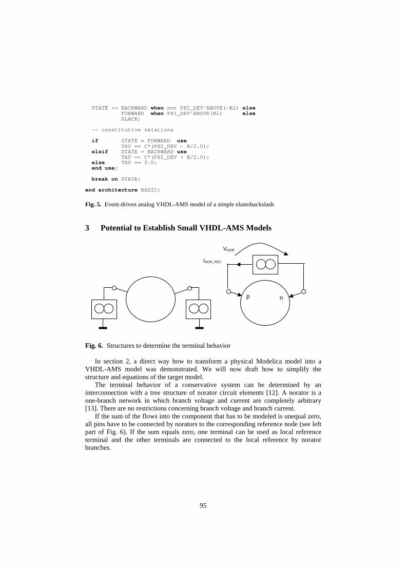
STATE <= BACKWARD when not PHI_DEV'ABOVE(-B2) else FORWARD when PHI_DEV'ABOVE(B2) else SLACK; -- constitutive relations if STATE = FORWARD use TAU == C*(PHI_DEV – B/2.0); elsif STATE = BACKWARD use TAU == C*(PHI_DEV + B/2.0); else TAU == 0.0; end use; break on STATE; end architecture BASIC;

Fig. 5. Event-driven analog VHDL-AMS model of a simple elastobackslash

3 Potential to Establish Small VHDL-AMS Models

Fig. 6. Structures to determine the terminal behavior

In section 2, a direct way how to transform a physical Modelica model into a VHDL-AMS model was demonstrated. We will now draft how to simplify the structure and equations of the target model.

The terminal behavior of a conservative system can be determined by an interconnection with a tree structure of norator circuit elements [12]. A norator is a one-branch network in which branch voltage and current are completely arbitrary [13]. There are no restrictions concerning branch voltage and branch current.

If the sum of the flows into the component that has to be modeled is unequal zero, all pins have to be connected by norators to the corresponding reference node (see left part of Fig. 6). If the sum equals zero, one terminal can be used as local reference terminal and the other terminals are connected to the local reference by norator branches.

VNOR

INOR_REV

p n

95

The structure of the final model is the same as the structure of the norator tree(s). The analysis of the test structure delivers the model equations that are expressed with the branch quantities of the norator branches.

Example

Let us have a look at the Modelica model from Table 2. The sum of the currents p.i and n.i is 0.0 (see the equations of the partial model OnePort). Thus, we can use a test circuit similar to the right part of Fig. 6. The network equations are given by

⎟⎟⎟⎟⎟⎟⎟⎟⎟⎟⎟

⎠

⎞

⎜⎜⎜⎜⎜⎜⎜⎜⎜⎜⎜

⎝

⎛

=

⎟⎟⎟⎟⎟⎟⎟⎟⎟⎟⎟

⎠

⎞

⎜⎜⎜⎜⎜⎜⎜⎜⎜⎜⎜

⎝

⎛

⋅

⎟⎟⎟⎟⎟⎟⎟⎟⎟⎟

⎠

⎞

⎜⎜⎜⎜⎜⎜⎜⎜⎜⎜

⎝

⎛

−−−

−−

−−

00000000

....

1...1...1....1...1....11..1......1..1......11.....1..11

_ REVNOR

NOR

IV

ivinipvnvp

R (2)

The first four equations represent the equation part of the Modelica model from Table 2. The last three equations result from the Kirchhoff laws. There is no additional constitutive relation that restricts branch voltage and current of the norator. Thus, there are fewer equations than unknowns.

These equations (2) can easily be transformed (for instance using a row echelon algorithm) into the following form

⎟⎟⎟⎟⎟⎟⎟⎟⎟⎟⎟

⎠

⎞

⎜⎜⎜⎜⎜⎜⎜⎜⎜⎜⎜

⎝

⎛

=

⎟⎟⎟⎟⎟⎟⎟⎟⎟⎟⎟

⎠

⎞

⎜⎜⎜⎜⎜⎜⎜⎜⎜⎜⎜

⎝

⎛

⋅

⎟⎟⎟⎟⎟⎟⎟⎟⎟⎟

⎠

⎞

⎜⎜⎜⎜⎜⎜⎜⎜⎜⎜

⎝

⎛

−−−

−−−

00000000

....

........1......

1.1.......1....

1...1...1....1..

.....11

_ REVNOR

NOR

IV

ivinipvnvp

R

R

R

(3)

The constitutive relation of the model only depends on the equations that now

restrict the branch voltage and current VNOR and INOR_REV resp. in the norator branch

0_ =⋅− REVNORNOR IRV (4)

This equation and the used norator structure are the basis of the architecture A0 of the VHDL-AMS model in Table 2.

We will try to outline the general procedure that was applied in the example:

96

1. Starting point is a physical (conservative) Modelica model. 2. Combine pins in one group if the sum of the associated flows equals zero. 3. Select a local reference pin in each group. Connect all other pins of the group with

the associated reference pin by norator branches. Connect the remaining pins by norator branches with the associated global reference node. In the norator branches, voltages and currents are contrarily counted.

4. Establish the network equations of the designed test circuit 0),)'(),(( =ttxtxF (5)

with mnn RRRRF →×× +: and nRRx →+:

5. Try to transform this equations into

0)),('),('),('),(),(),(( 3213211 =ttxtxtxtxtxtxF (6.1) 0)),('),('),(),(( 32322 =ttxtxtxtxF (6.2)

with 1321321:1mnnnnnn RRRRRRRRF →×××××× +

23232:2mnnnn RRRRRRF →×××× +

1:1nRRx →+ , 2:2

nRRx →+ , 3:3nRRx →+

All norator branch voltages and currents are summarized in x3.

6. If 23

22n

nm += , a VHDL-AMS model can be established. The internal branch

structure of the model is given by the structure of the norator branches and their voltage directions. Additional free quantities that represent the x2 waveforms must be declared in the architecture. The simultaneous statements of the model are given by F2.

7. In a final step the VHDL-AMS model has to be checked against the Modelica model.

The procedure cannot only be applied to a basic model but also to an

interconnection of models. It can be simplified if the transformation of the equations (5) into (6.1) and (6.2) can make use of the facilities of a simulator. This requires access to the reduced equations created by the simulator.

The transformation from VHDL-AMS to Modelica can be done in a similar way.

4 Conclusions

Some aspects of the transformation of Modelica models into VHDL-AMS descriptions were discussed.

A pure code-based transformation will not deliver the expected quality in a lot of cases. A method was prototyped how the transformation could be supported by analyzing appropriated test circuits. This could be a basis for a model transformation process if the reduced equations are available as a result of the evaluation of a Modelica description. The availability of differential algebraic equations that are

97

established by the simulation program would offer a lot of opportunities concerning model transformation. This is also valid for a transformation from VHDL-AMS to Modelica.

Many other aspects of model transformation could not be taken into consideration in this paper in detail. A special problem is the handling of initial values for instance. There are a lot of facilities in Modelica (for instance based on the experiences with index problems of mechanical system analysis). VHDL-AMS offers a solution based on the experiences with operating point analysis of electronic circuits.

An exchange of models between the two languages should not bring up problems in principle. However, a full automatic transformation of models seems only possible under special conditions.

Acknowledgement

The authors would like to thank the referees for helpful comments.

References

1. IEEE standard VHDL analog and mixed-signal extensions. IEEE DASC, December 1999 (revised May 2007). Online: http://www.designers-guide.org/Modeling

2. Modelica – A Unified Object-Oriented Language for Physical Systems Modeling. Language Specification. Version 2.2, Modelica Association, February 2005. Online:

http://www.modelica.org 3. Verilog-AMS Language Reference Manual. Version 2.2. Accellera, November 2004.

Online: http://www.eda.org/verilog-ams 4. Vachoux, A.; Grimm, C.; Einwich, K.: SystemC-AMS Requirements, Design Objects and

Rationale. Proc. DATE ’03, Munich, March 2003, pp. 388-393. Online: http://www.systemc-ams.org

5. Nagel, L. W.; Pederson D. O: SPICE2 – Simulation program with integrated circuits emphasis. Univ. of California, ERL-Memo M520, 1975.

6. Vlach, M.: Modeling And Simulation with Saber. Proc. 3rd Annual IEEE ASIC Seminar, September 1990, pp. 17-21.

7. Brenan, K.E.; Campbell, S.L.; Petzold, L.R.: Numerical Solution of Initial-Value Problems in Differential-Algebraic Equations. North-Holland, 1989.

8. Haase, J.: Rules for Analog and Mixed-Signal VHDL-AMS Modeling. In Grimm, C. (ed.): Languages for System Specification. Kluwer Academic Publishers, 2004, pp. 169 – 182.

9. Ho, C.-W.; Ruehli, A.; Brennan, P.: The modified nodal approach to network analysis. IEEE Trans. Circ. Syst. 22(1975)6, pp. 504-509.

10. Fritzson, P.: Principles of Object-Oriented Modeling and Simulation with Modelica 2.1. IEEE Press, 2004.

11. Lallement, C.; Pecheux, F.; Vachoux, A.; Prégaldiny, F. : Compact Modeling of the MOSFET in VHDL-AMS. In Grabinski, W.; Nauwelaers, B.; Schruers, D.: Transistor Level Modeling for Analog/RF IC Design. Springer-Verlag, 2006, pp. 243-269. Online: http://lsmwww.epfl.ch/models/compact/

12. Reibiger, A.: On the terminal behavior of networks. Proc. ECTD ’85, Prague, 1985, pp. 224-227.

13. Carlin, H. J.; Youla, D. C.: Network synthesis with negative resistors. Proc. IRE 49 (1961) 5, pp. 907-920.

98

Modeling Structural - Dynamics Systems in MODELICA/Dymola,

MODELICA/Mosilab and AnyLogic

Günther Zauner1,2, Daniel Leitner3, Felix Breitenecker1

1Vienna University of Technology, Wiedner Hauptstr. 8-10, 1040 Vienna, Austria

2Drahtwarenhandlung – Simulation Services, Neustiftgasse 57-59, 1070 Vienna 3Austrian Research Centers GmbH – ARC, Biomedical Engineering,

Donau-City Straße 1/8, 1220 Vienna guenther.zauner@drahtwarenhandlung.at

Abstract. With the progress in modeling dynamic systems new extensions in model coupling are needed. The models in classical engineering are described by differential equations. Depending on the general condition of the system the description of the model and thereby the state space is altered. This change of system behavior can be implemented in different ways. In this work we focus on three state-of-the-art DAE simulation environments, Dymola, Mosilab and AnyLogic, and compare the possibilities of coupling of different state spaces. This can be done either using a parallel model setup, a serial model setup, or a combined model setup. The analogies and discrepancies are figured out on the basis of the classical constrained pendulum as defined in ARGESIM comparison C7.

Keywords: Structural dynamics, state charts, Dymola, Mosilab, AnyLogic

1 Introduction

In the last decade the increase of computer power and the apace growth of model complexity leads to a new generation of simulation environments. Concurrently ambitions pointed towards establishing standardization. Especially the Modelica organization develops a wide range of syntax description and standard libraries.

This paper will compare the solutions of the constrained pendulum as an easy to model example, implemented in the most common Modelica simulator Dymola, Mosilab, a product from six Fraunhofer Institutes which uses Modelica syntax with extensions for state charts, and the simulator AnyLogic from Xjtek in St.Petersburg. This simulator also has object oriented structure and is fully implemented in JAVA.

We will focus on how the model can be implemented and we will have a look in which time slot the state events are and if there is a significant difference referring to the implementation method.

99

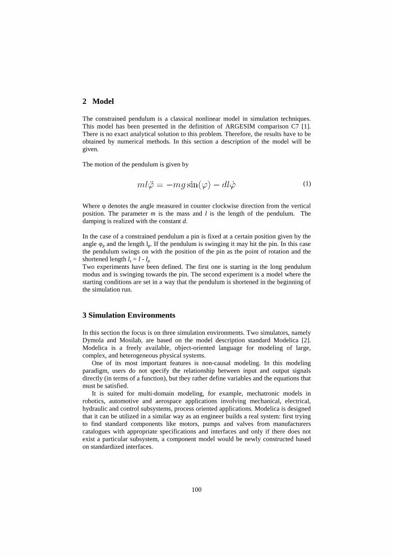
2 Model

The constrained pendulum is a classical nonlinear model in simulation techniques. This model has been presented in the definition of ARGESIM comparison C7 [1]. There is no exact analytical solution to this problem. Therefore, the results have to be obtained by numerical methods. In this section a description of the model will be given.

The motion of the pendulum is given by

(1)

Where φ denotes the angle measured in counter clockwise direction from the vertical position. The parameter m is the mass and l is the length of the pendulum. The damping is realized with the constant d. In the case of a constrained pendulum a pin is fixed at a certain position given by the angle φp and the length lp. If the pendulum is swinging it may hit the pin. In this case the pendulum swings on with the position of the pin as the point of rotation and the shortened length ls = l - lp.

Two experiments have been defined. The first one is starting in the long pendulum modus and is swinging towards the pin. The second experiment is a model where the starting conditions are set in a way that the pendulum is shortened in the beginning of the simulation run.

3 Simulation Environments

In this section the focus is on three simulation environments. Two simulators, namely Dymola and Mosilab, are based on the model description standard Modelica [2]. Modelica is a freely available, object-oriented language for modeling of large, complex, and heterogeneous physical systems.

One of its most important features is non-causal modeling. In this modeling paradigm, users do not specify the relationship between input and output signals directly (in terms of a function), but they rather define variables and the equations that must be satisfied.

It is suited for multi-domain modeling, for example, mechatronic models in robotics, automotive and aerospace applications involving mechanical, electrical, hydraulic and control subsystems, process oriented applications. Modelica is designed that it can be utilized in a similar way as an engineer builds a real system: first trying to find standard components like motors, pumps and valves from manufacturers catalogues with appropriate specifications and interfaces and only if there does not exist a particular subsystem, a component model would be newly constructed based on standardized interfaces.

100

The actual version of the Modelica Standard Library is 2.2.1, which has been released in April 2006.

3.1 Dymola

Dymola, DYnamic MOdeling LAboratory, is an environment for modeling and simulation of integrated and complex systems. It has unique multi-engineering capabilities which mean that models can consist of components from many engineering domains.

The basic structure of the simulator is divided into two separate parts: the Modeling layer and the Simulation layer. Thereby the modeling layer is separated in three parts. One part, the so called ICON layer, is used to define the shape of the new defined blocks. The DIAGRAM layer is the interface for graphical modeling. The third plane is the MODELICA TEXT part where the Modelica source code can be implemented directly. Dymola has a strong focus on using symbolic methods for mass-matrix inversion and equation sorting.

Integration algorithms for non-real-time simulation typically handle discontinuities by detecting when certain variables cross a boundary. They then calculate the time of the event by iteration and then change the step size to advance the time exactly to the time of the event (crossing) [3].

The default integration method is the Dassl code as defined by Petzold. The method can also be freely chosen out of 15 standard solvers, including algorithms for stiff systems. There is until now no possibility implemented to make graphical model switching for subsystems with different state space dimension.

3.2 Mosilab

The simulator Mosilab (MOdeling and SImulation LABoratory) is an environment developed from the Fraunhofer-Institutes FIRST, IIS/EAS, ISE, IBP, IWU and IPK in the research project GENSIM.

It has been developed for time-continuous and time-discrete analysis of heterogeneous technical systems. The main innovation from point of simulation techniques view in this simulator is the illustration of condition-based changes in the model structure (model structure dynamics). With this mechanism it is possible develop and simulate models with different modeling depth.

The model description in general is done in the Modelica standard. Additional features to assure high flexibility during modeling and the concept of structural dynamics is implemented. This is done by extending the Modelica standard with state charts, controlling dynamic models. The extended object-oriented model description language resulting is called MOSILA [1,4] Moreover simulator coupling with standard tools (e.g. MATLAB / Simulink, FEMLAB) is realized.

101

Code generation is done in a quite similar way as in Dymola/Modelica. This makes sense, because this relatively new simulator will also be able to simulate problems defined in the standard Modelica notation with other tools, which use the same syntax. The main difference is the extension for graphical representation of state charts. This is solved with an interface where the user can define UML state charts.

The analysis part of the model is split into two layers: the simulation and the post

processing layer. The defined code is translated into C++. The default integration method is the so called idadassl. Other implemented methods are for example the implicit trapeze method and the explicit or implicit euler.

3.3 AnyLogic

AnyLogic is a multiparadigm simulator supporting Agent Based modeling as well as Discrete Event modeling, which is flowchart-based, and System Dynamics, which is a stock-and-flow kind of description. Due to its very high flexibility AnyLogic is capable of capturing arbitrary complex logic, intelligent behavior, spatial awareness and dynamically changing structures. It is possible to combine different modeling approaches making AnyLogic a hybrid simulator. AnyLogic is highly object oriented and based on the Java programming language. To a certain degree this ensures a compatibility and reusability of the resulting models. The development of AnyLogic in the last years has been towards business simulation. In version 6 of AnyLogic it is possible to calculate problems from engineering, but there are certain restrictions. For example the integration method cannot be chosen freely and there is no state event finder. When a model starts, the equations are assembled into the main differential equation system. During the simulation, this DES is solved by one of the numerical methods built in AnyLogic. AnyLogic provides a set of numerical methods for solving ordinal differential equations (ODE), algebraic-differential equations (DAE), or algebraic equations (NAE). AnyLogic chooses the numerical solver automatically at runtime in accordance to the behavior of the system. When solving ordinal differential equations, it starts integration with forth-order Runge-Kutta method with fixed step. Otherwise, AnyLogic plugs in another solver – Newton method. This method changes the integration step to achieve the given accuracy.

102

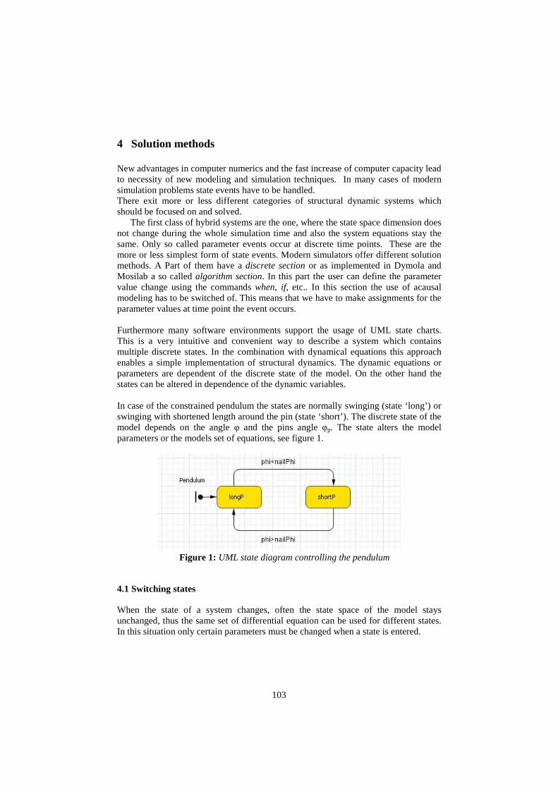
4 Solution methods

New advantages in computer numerics and the fast increase of computer capacity lead to necessity of new modeling and simulation techniques. In many cases of modern simulation problems state events have to be handled. There exit more or less different categories of structural dynamic systems which should be focused on and solved.

The first class of hybrid systems are the one, where the state space dimension does not change during the whole simulation time and also the system equations stay the same. Only so called parameter events occur at discrete time points. These are the more or less simplest form of state events. Modern simulators offer different solution methods. A Part of them have a discrete section or as implemented in Dymola and Mosilab a so called algorithm section. In this part the user can define the parameter value change using the commands when, if, etc.. In this section the use of acausal modeling has to be switched of. This means that we have to make assignments for the parameter values at time point the event occurs.

Furthermore many software environments support the usage of UML state charts. This is a very intuitive and convenient way to describe a system which contains multiple discrete states. In the combination with dynamical equations this approach enables a simple implementation of structural dynamics. The dynamic equations or parameters are dependent of the discrete state of the model. On the other hand the states can be altered in dependence of the dynamic variables. In case of the constrained pendulum the states are normally swinging (state ‘long’) or swinging with shortened length around the pin (state ‘short’). The discrete state of the model depends on the angle φ and the pins angle φp. The state alters the model parameters or the models set of equations, see figure 1.

Figure 1: UML state diagram controlling the pendulum

4.1 Switching states

When the state of a system changes, often the state space of the model stays unchanged, thus the same set of differential equation can be used for different states. In this situation only certain parameters must be changed when a state is entered.

103

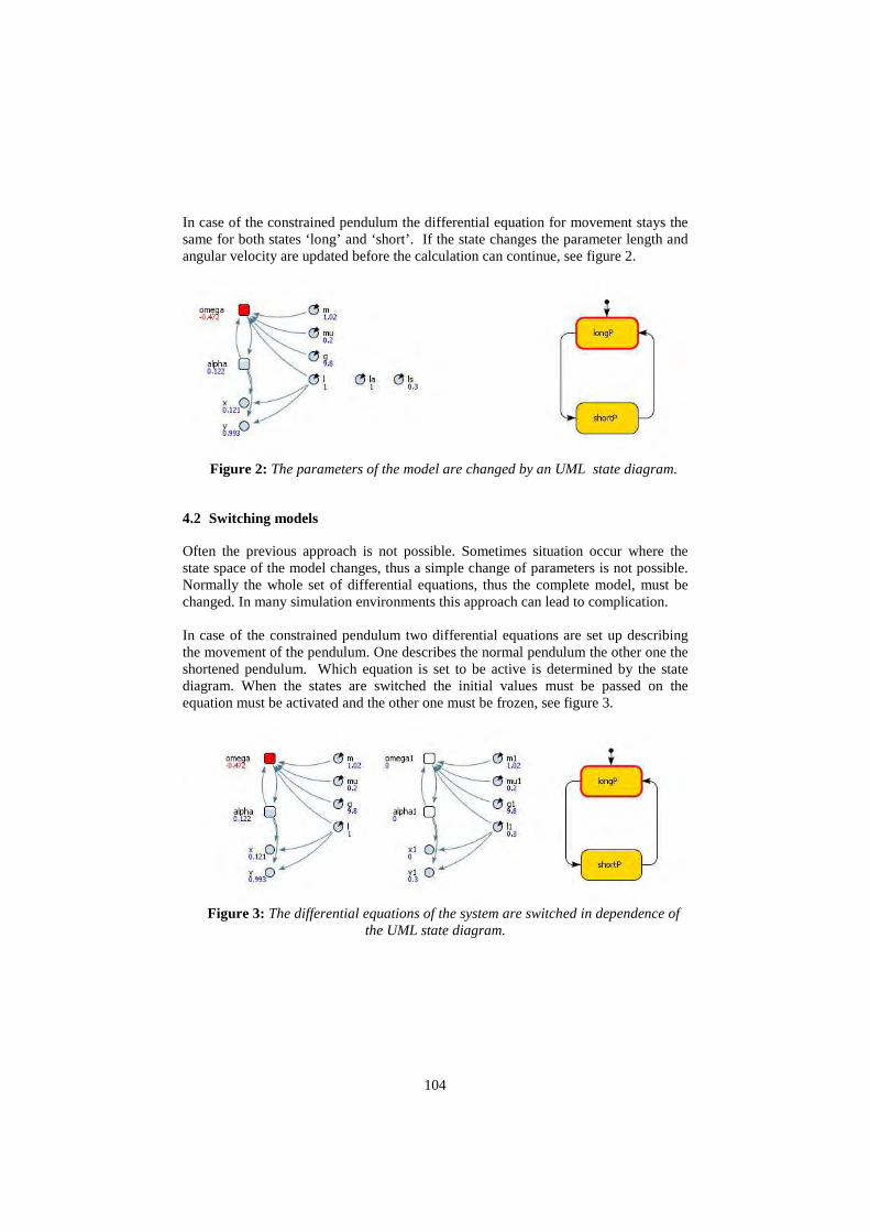
In case of the constrained pendulum the differential equation for movement stays the same for both states ‘long’ and ‘short’. If the state changes the parameter length and angular velocity are updated before the calculation can continue, see figure 2.

Figure 2: The parameters of the model are changed by an UML state diagram.

4.2 Switching models

Often the previous approach is not possible. Sometimes situation occur where the state space of the model changes, thus a simple change of parameters is not possible. Normally the whole set of differential equations, thus the complete model, must be changed. In many simulation environments this approach can lead to complication. In case of the constrained pendulum two differential equations are set up describing the movement of the pendulum. One describes the normal pendulum the other one the shortened pendulum. Which equation is set to be active is determined by the state diagram. When the states are switched the initial values must be passed on the equation must be activated and the other one must be frozen, see figure 3.

Figure 3: The differential equations of the system are switched in dependence of

the UML state diagram.

104

5 Dymola

The implementation of the constrained pendulum has been done in two more or less different ways. As Dymola does not support the UML – notation for state charts and there is in the moment no method implemented to switch between two or more independent models during one simulation run, the solution methods described in section 4.1 and 4.2 can not be used. In our example the state event, which appears every time when the rope of the pendulum hits the pin or looses the connection to it, is modeled in an algorithm section. This can be done with the following code digest:

algorithm

if (phi<=phipin) then

length:=ls;

end if;

if (phi>phipin) then

length:=l1;

end if;

Another method for implementing the constrained pendulum in Dymola is the use of standard blocks in combination with a predefined model which includes the equations or using only the Modelica.Blocks components.

In this example the solution is made by using standard blocks with little extension. Figure 4 shows a screenshot of the Diagram layer of this model.

Figure 4: The screenshot of the Diagram layer in Dymola/Modelica

The main difference is that no algorithm section is used in the model. The lower

part of the system shown in figure 4 is solved with Modelica.StateGraph library.

105

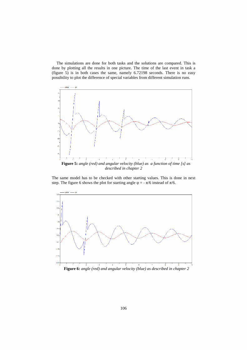
The simulations are done for both tasks and the solutions are compared. This is done by plotting all the results in one picture. The time of the last event in task a (figure 5) is in both cases the same, namely 6.72198 seconds. There is no easy possibility to plot the difference of special variables from different simulation runs.

Figure 5: angle (red) and angular velocity (blue) as a function of time [s] as

described in chapter 2

The same model has to be checked with other starting values. This is done in next step. The figure 6 shows the plot for starting angle φ = - π/6 instead of π/6.

Figure 6: angle (red) and angular velocity (blue) as described in chapter 2

106

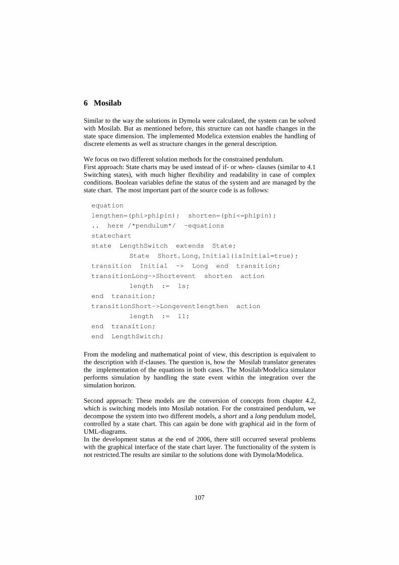
6 Mosilab

Similar to the way the solutions in Dymola were calculated, the system can be solved with Mosilab. But as mentioned before, this structure can not handle changes in the state space dimension. The implemented Modelica extension enables the handling of discrete elements as well as structure changes in the general description. We focus on two different solution methods for the constrained pendulum. First approach: State charts may be used instead of if- or when- clauses (similar to 4.1 Switching states), with much higher flexibility and readability in case of complex conditions. Boolean variables define the status of the system and are managed by the state chart. The most important part of the source code is as follows: equation

lengthen=(phi>phipin); shorten=(phi<=phipin);

.. here /*pendulum*/ -equations

statechart

state LengthSwitch extends State;

State Short,Long,Initial(isInitial=true);

transition Initial -> Long end transition;

transitionLong->Shortevent shorten action

length := ls;

end transition;

transitionShort->Longeventlengthen action

length := l1;

end transition;

end LengthSwitch;

From the modeling and mathematical point of view, this description is equivalent to the description with if-clauses. The question is, how the Mosilab translator generates the implementation of the equations in both cases. The Mosilab/Modelica simulator performs simulation by handling the state event within the integration over the simulation horizon. Second approach: These models are the conversion of concepts from chapter 4.2, which is switching models into Mosilab notation. For the constrained pendulum, we decompose the system into two different models, a short and a long pendulum model, controlled by a state chart. This can again be done with graphical aid in the form of UML-diagrams. In the development status at the end of 2006, there still occurred several problems with the graphical interface of the state chart layer. The functionality of the system is not restricted.The results are similar to the solutions done with Dymola/Modelica.

107

7 AnyLogic

The implementation of the constrained pendulum has been done in two different ways. In the first approach only the parameter states have been switched corresponding to section 4.1, in the second approach the whole differential equation is switched corresponding to section 4.2. Both examples from chapter 2 have been calculated with both approaches. The results in AnyLogic are identical in both methods because the times of the state transitions are the same. In the first approach the model consists of two ordinary differential equations describing the movement of the pendulum. In these equations four parameters are used length l, mass m, damping d, and gravity g. Further a state diagram with states ‘long’ and ‘short’ and two transitions are used to update the equations. When the state changes length l and angular velocity ω are updated. The results calculated by AnyLogic 6 are plotted in figure 7 and figure 8.

Figure 7: Results for example 1: angle (red), angular velocity (blue)

The second approach uses two separate models. The implemented model consists of two times two ordinary differential equations. Both equations have four parameters separately: length l, mass m, damping d, and gravity g. A state diagram is implemented analog to the first approach. If the state changes the right differential equations are activated and their initial values are set, while the other differential equation is frozen.

108

Figure 8: Results for example 2: angle (red), angular velocity (blue)

8 Discussion

For this nonlinear model, there exists no exact solution. For this reason we can only calculate the numerical solutions and compare, for example, the time points where the last state event appears. This is the moment when the rope of the pendulum looses the connection to the pin the last time. In the first model under investigation, this happens after the fourth time shortening the pendulum, which means after eight state events all together. In the second simulation run, this occurs earlier, namely already after two times lengthening the rope, which means after three state events, because of the special initial condition (pendulum is in short modus at starting time).

The solutions are calculated with the default simulation method, if possible. With this approach we try to test the simulation environments from the user’s point of view. Many programmers and modelers do not care that much about the implemented integration methods. For this reason the standard method has to produce reliable results in an appropriate calculation time.

The solution in the Mosilab simulator with standard Modelica components cannot be calculated with the standard method (Dassl code), because during simulation of this task a numerical error occurs and therefore the calculation is interrupted. The integration method pins at the time point of the first state event. Because of this reason the Implicit Trapez method was chosen. The other results are all done with the standard integration method and the given step sizes/number of intervals.

109

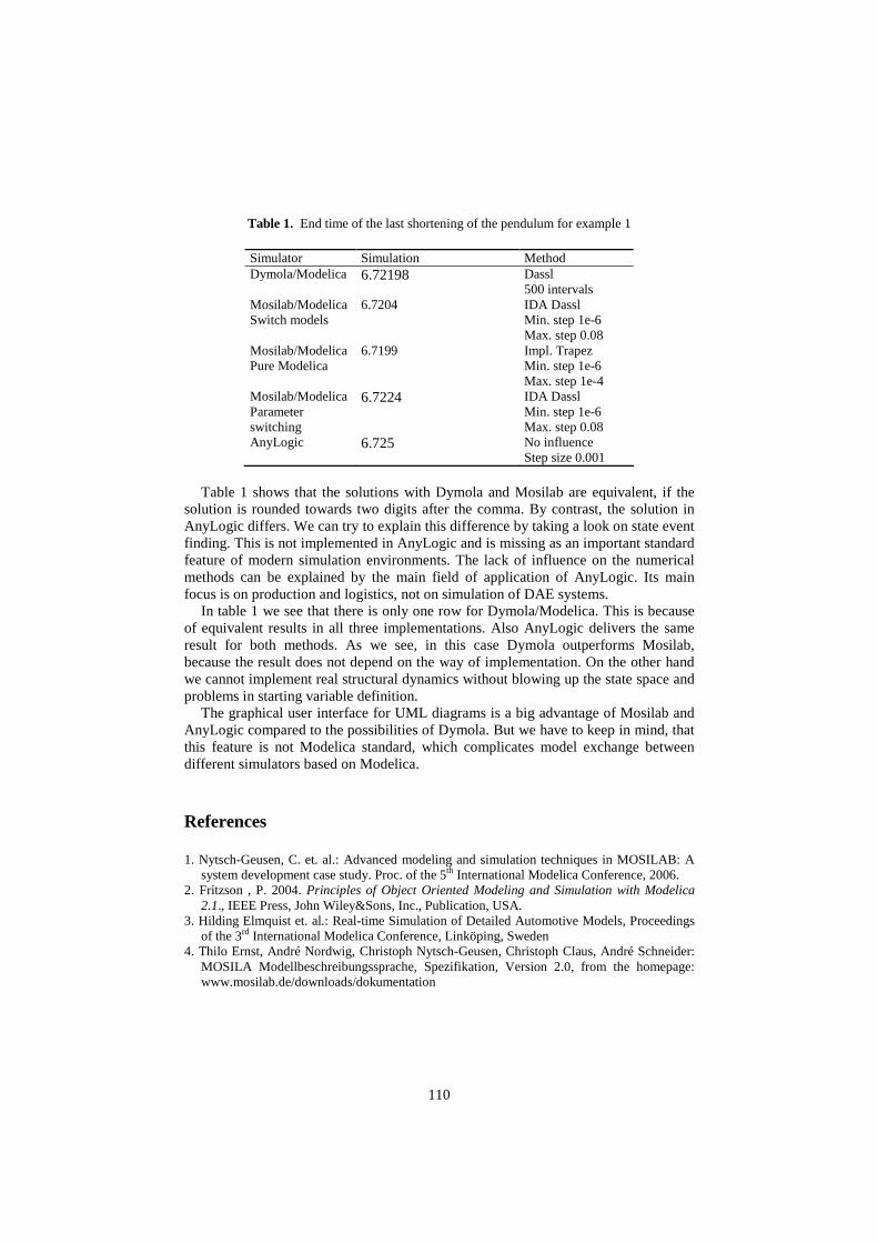
Table 1. End time of the last shortening of the pendulum for example 1

Simulator Simulation Method Dymola/Modelica 6.72198 Dassl

500 intervals Mosilab/Modelica Switch models

6.7204 IDA Dassl Min. step 1e-6 Max. step 0.08

Mosilab/Modelica Pure Modelica

6.7199 Impl. Trapez Min. step 1e-6 Max. step 1e-4

Mosilab/Modelica Parameter switching

6.7224 IDA Dassl Min. step 1e-6 Max. step 0.08

AnyLogic 6.725 No influence Step size 0.001

Table 1 shows that the solutions with Dymola and Mosilab are equivalent, if the

solution is rounded towards two digits after the comma. By contrast, the solution in AnyLogic differs. We can try to explain this difference by taking a look on state event finding. This is not implemented in AnyLogic and is missing as an important standard feature of modern simulation environments. The lack of influence on the numerical methods can be explained by the main field of application of AnyLogic. Its main focus is on production and logistics, not on simulation of DAE systems.

In table 1 we see that there is only one row for Dymola/Modelica. This is because of equivalent results in all three implementations. Also AnyLogic delivers the same result for both methods. As we see, in this case Dymola outperforms Mosilab, because the result does not depend on the way of implementation. On the other hand we cannot implement real structural dynamics without blowing up the state space and problems in starting variable definition.

The graphical user interface for UML diagrams is a big advantage of Mosilab and AnyLogic compared to the possibilities of Dymola. But we have to keep in mind, that this feature is not Modelica standard, which complicates model exchange between different simulators based on Modelica.

References

1. Nytsch-Geusen, C. et. al.: Advanced modeling and simulation techniques in MOSILAB: A system development case study. Proc. of the 5th International Modelica Conference, 2006.

2. Fritzson , P. 2004. Principles of Object Oriented Modeling and Simulation with Modelica 2.1., IEEE Press, John Wiley&Sons, Inc., Publication, USA.

3. Hilding Elmquist et. al.: Real-time Simulation of Detailed Automotive Models, Proceedings of the 3rd International Modelica Conference, Linköping, Sweden

4. Thilo Ernst, André Nordwig, Christoph Nytsch-Geusen, Christoph Claus, André Schneider: MOSILA Modellbeschreibungssprache, Spezifikation, Version 2.0, from the homepage: www.mosilab.de/downloads/dokumentation

110

Abstract Syntax Can Makethe Definition of Modelica Less Abstract

David Broman and Peter Fritzson

Department of Computer and Information ScienceLinkoping University, Sweden

davbr,petfr@ida.liu.se

Abstract. Modelica is an open standardized language used for model-ing and simulation of complex physical systems. The language specifi-cation defines a formal concrete syntax, but the semantics is informallydescribed using natural language. The latter makes the language hardto interpret, maintain and reason about, which affect both tool develop-ment and language evolution. Even if a completely formal semantics ofthe Modelica language can be seen as a natural goal, it is a well-knownfact that defining understandable and concise formal semantics specifi-cations for large and complex languages is a very hard problem. In thispaper, we will discuss different aspects of formulating a Modelica specifi-cation; both in terms of what should be specified and how it can be done.Moreover, we will further argue that a ”middle-way” strategy can makethe specification both clearer and easier to reason about. A proposalis outlined, where the current informally specified semantics is comple-mented with several grammars, specifying intermediate representationsof abstract syntax. We believe that this kind of evolutionary strategy iseasier to gain acceptance for, and is more realistic in the short-term, thana revolutionary approach of using a fully formal semantics definition ofthe language.

1 Introduction

Modelica is an open standard language aimed primarily at modeling and sim-ulation of complex physical systems. The first language specification 1.0 [19]was released in September 1997. Since then, the current specification 2.2[20] hasevolved to be large and complex with many constructs.

During these past ten years, the user community has grown fairly large andthe Modelica Standard Library has evolved to include several physical domains.The dominating Modelica tool has for a long time been the commercial toolDymola [4]. However, during recent years, alternative tools have emerged; bothopen source (OpenModelica [7, 21]) and commercial environments (e.g., Math-Modelica System Designer [16], MOSILAB [5], and SimulationX[12]).

The rapidly growing user community and increasing number of tool vendorsaugment the demand of the language specification being precise so that different

111

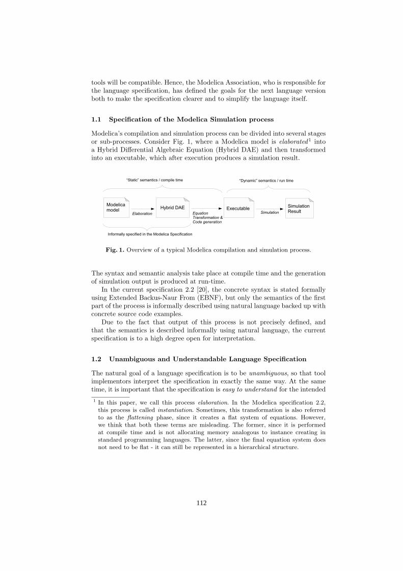
tools will be compatible. Hence, the Modelica Association, who is responsible forthe language specification, has defined the goals for the next language versionboth to make the specification clearer and to simplify the language itself.

1.1 Specification of the Modelica Simulation process

Modelica’s compilation and simulation process can be divided into several stagesor sub-processes. Consider Fig. 1, where a Modelica model is elaborated1 intoa Hybrid Differential Algebraic Equation (Hybrid DAE) and then transformedinto an executable, which after execution produces a simulation result.

Fig. 1. Overview of a typical Modelica compilation and simulation process.

The syntax and semantic analysis take place at compile time and the generationof simulation output is produced at run-time.

In the current specification 2.2 [20], the concrete syntax is stated formallyusing Extended Backus-Naur From (EBNF), but only the semantics of the firstpart of the process is informally described using natural language backed up withconcrete source code examples.

Due to the fact that output of this process is not precisely defined, andthat the semantics is described informally using natural language, the currentspecification is to a high degree open for interpretation.

1.2 Unambiguous and Understandable Language Specification

The natural goal of a language specification is to be unambiguous, so that toolimplementors interpret the specification in exactly the same way. At the sametime, it is important that the specification is easy to understand for the intended

1 In this paper, we call this process elaboration. In the Modelica specification 2.2,this process is called instantiation. Sometimes, this transformation is also referredto as the flattening phase, since it creates a flat system of equations. However,we think that both these terms are misleading. The former, since it is performedat compile time and is not allocating memory analogous to instance creating instandard programming languages. The latter, since the final equation system doesnot need to be flat - it can still be represented in a hierarchical structure.

112

audience. Unfortunately, it is not that easy to meet both of these goals whendescribing a large and complex modeling language such as Modelica. There areseveral specification approaches with different pros and cons. Hence, the overallproblem is to find an approach that satisfies the specification goals in the bestpossible way.

If the language is described using formal semantics, e.g., structured opera-tional semantics [25], the language semantics is precise and can in some casesbe proved to have certain properties, such as type safety [24, 26]. However, tounderstand and interpret a formal language specification require a rigorous the-oretical computer science knowledge. Furthermore, even if great effort has beenspent during the last decades in formalizing mainstream programing languages,only a few, e.g., Standard ML [18], are actually fully formally specified. Accord-ingly, it turns out to be a very hard task to specify an understandable and conciseformal specification of an existing complex language.

Alternatively, if the language semantics is described using natural languages,e.g., plain English text describing the semantics, it might be easy for softwareengineers to understand the specification. Many languages are described in thisway, for example Java [9], C++ [11], and Modelica [20]. However, ease of un-derstanding does not imply that different individuals interpret the specificationin the same way. It is a well known fact that it is very hard to write unam-biguous natural language specifications, and perhaps even harder to verify theirconsistency.

1.3 Previous Specification Attempts

Several previous attempts have been made to formalize and improve the spec-ification of the Modelica language. The most obvious one is the further devel-opment of the official language specification itself, conducted by the ModelicaAssociation. The work on the next language specification includes substantialrestructuring and a more detailed description of the semantics of the language.However, it is not planned to include any formal descriptions, apart from anappendix containing one possible definition of Modelica abstract syntax.

Natural Semantics. Already in 1998 Kagedal and Fritzson [14, 15], createda formal specification for a subset of the Modelica language, influenced by thelanguage specification examples described in the 1997 version of [6]. The speci-fication was using Natural Semantics [13] and the executable specification lan-guage Relational Meta Language (RML) [22]. This work influenced the designof the language and the official Modelica specification. The executable specifi-cation has gradually evolved and is now the code basis for the OpenModelicaproject[21]. In 2006, the code base was converted from RML to Meta-Modelica[8]with the purpose of making it more accessible for software engineers in the Mod-elica community. Hence, today the project is more intended to be a completeimplementation of the language than a specification itself. One lesson learnedfrom this specification project was that for an almost complete specification of

113

an early Modelica language version, the formal specification became hard to getan overview of, since it grew to be very large.

Elaboration. Jakob Mauss has made several contributions to formally describethe elaboration process (called instance creation in his work) of a subset of Mod-elica, i.e., the translation process from a Modelica model into a system of equa-tions. The published work [17] describes an algorithmic specification approach,which focuses on Modelica’s complex lookup rules and modification semantics;including redeclaration of classes and components. Semantics for describing re-strictions on validity of a model, such as types, restricted classes, and mostprefixes are not considered. It exists also a refined version of this work, whichuses a more compact notation. However, this work is still unpublished.

Modelica Types. In our previous work on types in the Modelica language[2],we concluded that the type concept is only implicitly defined in the Modelicalanguage specification. In that work, we proposed a concrete syntax of specifyingModelica types and gave a suggestion for constraining information of elementprefixes in the types. Furthermore, it was emphasized that Modelica has a struc-tural type system, which implies that a class and a type are two separate languageconcepts. In this paper, we will not cover types, even though parts of a specifi-cation can also be described using type rules.

A common dominator for all these isolated formal specification attempts is thatthey have been conducted in parallel with the official language specification. Evenif a proposed alternative specification covers large portions of the language, itwill not be used as a specification by the community if it is not replacing theofficial specification. If there are two specifications of the same concept, how dowe then know which one is valid if they are not consistent? Nevertheless, theseformal specification attempts are still very important to promote understandingand discussion about the informal semantics. It is of great importance that theseworks gradually find their way into the official specification. The question is howto make this possible in practice, since all attempts so far only model subsets ofthe real language.

1.4 Abstract Syntax as a Middle-Way Strategy

Improving the natural language description of the Modelica specification is anobvious way of increasing the understandability and removing ambiguity. How-ever, since this process is tedious and error prone, it is very hard to ensure thatthe ambiguity decreases. Moreover, previous work on formalization of the com-plete semantics of subsets of the language has shown to be complex and resultingin very large specifications. Hence, there is a concrete and practical need to finda ”middle-way” strategy to improve the clarity of the complete language, not justsubsets. This strategy must be simple enough to not require in depth theoreti-cal computer science knowledge of the reader, but still precise enough to avoidambiguities.

114

When a compiler parses a model, the result is normally stored internally asan Abstract Syntax Tree (AST). Hence, one particular model results in a specificAST, which can be seen as an instance of the language’s abstract syntax. Theabstract syntax can be specified using a context-free grammar, and an AST canalso have a corresponding textual representation.

The internal representation of an AST is often seen as a tool implementationissue, and not as something that is defined in a language specification. Neverthe-less, in this paper we propose that the intermediate representations between thetransformation steps (recall Fig. 1) should be described by specifying its abstractsyntax.

However, specifying different forms of abstract syntax cannot replace thesemantic specification need in the transformation process, since the syntax onlydescribes the structure of a model, while the semantics states the meaning ofit. Hence, in the short term, this specification complements the current informalspecification, by clarifying exactly what both the input and the output structureof a transformation are.

By following this evolutionary strategy, the semantic description may then begradually more described using techniques such as Syntax-Directed TranslationSchemes (SDT)[1] or different forms of operational semantics. However, as earlierdescribed, this is not straight forward when considering the whole Modelicalanguage. The main purposes of including abstract syntax definitions in thespecification can be summarized to be:

1. Specifying Valid Input. Increase the clarity of what valid Modelica actu-ally is, i.e, to make sure that different tools reject the same models.

2. Specifying Expected Output. Remove confusion of what the actual out-come of executing a Modelica model is.

3. Promoting Language Simplification. The Modelica language has beenidentified to be sometimes more complicated than necessary (e.g., relationsbetween the general class and restricted classes). An abstract syntax for-mulation can be used as a guidance tool for identifying the most usefulreformulations needed.

Part of the first item is already specified using the concrete grammar. To increasethe level of details that can be specified of the abstract syntax, we will later in thepaper suggest an informal approach to include context-sensitive information inthe abstract grammar specification. This rules out parts of the informal semanticsused for rejecting invalid models. However, great parts of the rejecting semanticsmust still be described using another semantic specification form.

In the following sections, we will gradually introduce more motivations anddescriptions of the abstract syntax approach. Section 2 gives an overview ofdifferent aspects of specifying a language specification in the context of Modelica.The discussion on different specification alternatives and aspects forms the basisfor Section 3, which more concretely elaborates on our proposal. Finally, inSection 4 concluding remarks are stated and future work is outlined.

115

2 Specifying the Modelica Specification

Defining a new language from scratch with an unambiguous and understand-able language specification is a difficult and time consuming task. Developingand enhancing a language over many years and still being able to keep thelanguage backwards compatible and the specification clear, is perhaps an evenmore challenging mission. In the previous section, we described this problemwith the current specification, motivated the need for improvement, and brieflyintroduced a proposed strategy. In the beginning of this section, we will focus onthe question what should actually be specified in the Modelica specification. Atthe end of the section, we will discuss how this specification can be achieved bysurveying some different specification approaches and compare how they relateto the abstract syntax approach.

At a high level, the syntax and semantics of Modelica can be divided intotwo main aspects:

– Transformation, i.e., the process of transforming a Modelica source codemodel into a well defined result. Depending on the purpose, the result caneither be an intermediate form of a Hybrid Differential Algebraic Equations(Hybrid DAE), or the final simulation result.

– Rejection, i.e., rules describing what a valid Modelica model actually is.These rules should unambiguously describe when a tool should reject theinput model as invalid.

Both these aspects are important for a clear-cut result, so that tool vendors cancreate compatible tools.

2.1 Transformation Aspects - What is Actually the Result of anExecution?

In the introduction section of the Modelica specification 2.2 [20], it is statedthat the scope of the specification is to define the semantics of the translationto a flat Hybrid DAE and that it does not define the result of a simulation. Amathematical notation of the hybrid DAE is given, but no precise and completeoutput is defined.

However, many constructs given in the specification are not handled duringthis translation to a Hybrid DAE. Hence, the semantics of these constructs (e.g.,when-equations, algorithm sections), are implicitly defined, even if the specifica-tion states that this should not be the case.

So, the questions arise: what is actually the transformation process? What isthe expected result of the execution? We would argue that the answer to thesequestions would differ depending on who you ask, since the current specifica-tion is open for interpretation. In this subsection, we give our view of a typicalModelica transformation process.

Recall Fig. 1, where the high-level view of a typical Modelica compilationand simulation process is outlined. The translation process is divided into threesub-processes, each having an artifact as input and output.

116

Elaboration. The elaboration process (also called instantiation and sometimesflattening) takes as input a source code Modelica model and transforms it into aHybrid DAE. This is the main part described in the Modelica specification, whichincludes among other things parsing, type checking, redeclarations, connectionelaboration, and generation of equations. The output is the Hybrid DAE, whichincludes items such as equations, function calls, algorithm sections, declarationof variables etc.

Equation Transformation and Code Generation The Hybrid DAE is sim-plified and transformed (index reduction, generation of Block Lower Triangularform (BLT)). Finally, target code is generated (typically C-code), which is linkedtogether with a numerical solver, such as DASSL[23].

Simulation The final transformation step is basically running the executable,where the actual simulation takes place. During this step, numerical integrationof the continuous system and discrete event handling occurs.

Static vs. Dynamic. In the example above, it was assumed that the processwas compiled and not interpreted. This is not a specification requirement, evenif it is common that tools are implemented as compilers. The definitions of sta-tic and dynamic semantics are often confusing in relation to compile-time andsimulation-time. Some people will argue that the dynamic semantics is only thesimulation sub-process and that the elaboration and equation transformation aswell as the code generation phases are the static semantics. If the tool is imple-mented as an interpreter, the distinction becomes less clear. In such a case, itis natural to view all three processes as the dynamic semantics. Even if this isonly a matter of definitions, it becomes significantly important when reasoningabout type checking and separate compilation.

From the discussion above, it is clear that we need to have a precise definitionof the input and the output of the elaboration process. Whether the two lastsub-processes should be part of the specification is an open design issue, butit is obviously important that the decision is made if it should be completelyincluded or removed.

2.2 Rejection Aspects - What is actually a Valid Modelica Model?

In the current specification, it is hard to interpret what valid Modelica inputis, i.e., it is difficult for a tool implementor to know which models that shouldbe rejected as invalid Modelica. A restrictive abstract syntax definition can helpclarifying several issues.

Besides specifying the translation semantics of a model, a language specifica-tion typically describes which models that should be treated as valid, and which

117

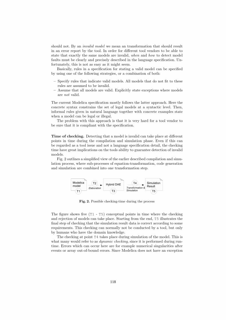
should not. By an invalid model we mean an transformation that should resultin an error report by the tool. In order for different tool vendors to be able tostate that exactly the same models are invalid, when and how to detect modelfaults must be clearly and precisely described in the language specification. Un-fortunately, this is not as easy as it might seem.

Basically, rules in a specification for stating a valid model can be specifiedby using one of the following strategies, or a combination of both:

– Specify rules that indicate valid models. All models that do not fit to theserules are assumed to be invalid.

– Assume that all models are valid. Explicitly state exceptions where modelsare not valid.

The current Modelica specification mostly follows the latter approach. Here theconcrete syntax constrains the set of legal models at a syntactic level. Then,informal rules given in natural language together with concrete examples statewhen a model can be legal or illegal.

The problem with this approach is that it is very hard for a tool vendor tobe sure that it is compliant with the specification.

Time of checking. Detecting that a model is invalid can take place at differentpoints in time during the compilation and simulation phase. Even if this canbe regarded as a tool issue and not a language specification detail, the checkingtime have great implications on the tools ability to guarantee detection of invalidmodels.

Fig. 2 outlines a simplified view of the earlier described compilation and simu-lation process, where sub-processes of equation-transformation, code generationand simulation are combined into one transformation step.

Fig. 2. Possible checking-time during the process

The figure shows five (T1 - T5) conceptual points in time where the checkingand rejection of models can take place. Starting from the end, T5 illustrates thefinal step of checking that the simulation result data is correct according to somerequirements. This checking can normally not be conducted by a tool, but onlyby humans who have the domain knowledge.

The checking at point T4 takes place during simulation of the model. This iswhat many would refer to as dynamic checking, since it is performed during run-time. Errors which can occur here are for example numerical singularities afterevents or array out-of-bound errors. Since Modelica does not have an exception

118

handling mechanism, it is implicitly assumed that the tool exits with an errorstatement. Checking point T3 is performed after the elaboration phase. This canfor example concern the control that the number of equations equals the numberof unknowns.

Even if it is not stated in the Modelica specification, T2 is our interpretationof the specification where the type checking takes place. Here, the naming ofthis kind of checking is often a source of confusion. If the elaboration phaseis regarded as the static semantics, some people call this static type checking.However, since the elaboration phase is the major part of the semantics describedin the specification, and it involves complex transformation semantics, this canbe viewed as something dynamic from an interpretive semantics point of view,or as something static from a translational semantics point of view. Using aninterpretive semantics style, T2 would involve dynamic type checking.

Following this argumentation, then T1 would represent static type checking,i.e., the types in the language are checked before elaboration. This reasoning isanalogous to dynamic checking in languages such as PHP and Common LISP,compared to static type checking in Haskell, Standard ML, or Java. Even if theModelica specification does not currently support this kind of static checking, ithas a major impact on the ability to detect and isolate for example over- andunder-constrained systems of equations[3] or to enable separate compilation.

2.3 Specification Approaches - How can we state what it’s allabout?

When it is clear what to specify, the next obvious question is how to specify it.There are several specification approaches, and we have briefly mentioned someof them earlier in this paper.

As evaluation criteria, it is natural to use the specification goals of under-standability2 and unambiguity. Furthermore, it is also of interest to estimate theexpressiveness of the approach, i.e., how much of the intended specification taskcan be covered by the approach.

In the following table, a number of possible specification approaches arelisted, with our judgements of the evaluation criteria.A natural language specification can be understandable and expressive, depend-ing on the size and quality of the text, but easily leads as we have discussed earlierto ambiguous specifications. Using a formal type system together with formalsemantics [24] is here seen as having low understandability, since it requires hightechnical training. It is however very precise and fairly expressive.

The expressiveness of the abstract syntax is stated as higher than the concretesyntax, since we can introduce context dependent information in the grammarusing meta-variables. An example of this will be given in the next section.

2 Understandability is of course a very subjective measurement. In this context, wehave chosen to also include the level of needed knowledge to understand the concept,i.e., a concept requiring an extensive computer science or mathematical backgroundresults in lower understandability rating.

119

Approach Understandability Expressiveness Unambiguous

Natural language description High-Medium High LowFormal semantics Low Medium HighAbstract Syntax Grammar Medium Medium HighConcrete Syntax Grammar Medium Low HighTest suite High High LowReference Implementation Low High High

Table 1. Possible specification approaches with estimated evaluation criteria.

We have also, for the sake of completeness, included related approaches such asthe use of a test suite and reference implementation. The approach to use a testsuite as a specification can be an interesting complement to abstract syntax andinformal semantics. However, it is very important to state which description thathas precedence if ambiguities are discovered. Finally, a reference implementationcan also be seen as a specification, even if it is hard to get an good overview andreason about it.

3 An Abstract Syntax Specification Approach

In the following section we will go into more details about the proposal to use ab-stract syntax as part of the Modelica specification. Initially, the different abstractsyntax representations are outlined in relation to the transformation process de-scribed in Section 2.1, followed by a discussion about the specification and rep-resentation of the syntax. Finally a small example of abstract syntax grammaris given and discussed.

3.1 Specifying the Elaboration Process

An Abstract Syntax Tree (AST) can be seen as a specific instance of an abstractsyntax. Transformation processes inside an compiler can be defined as transfor-mations from one intermediate representation to another. ASTs are a naturalform of intermediate representation.

Consider Fig. 3, where the elaboration process is shown with surroundingASTs. The first step in the process is the ordinary scanning and parsing step,

Fig. 3. Modelica’s compilation process divided into intermediate representations in theform of abstract syntax trees (ASTs).

120

which is formally defined in the specification using lexical definitions and concretesyntax definitions using Extended BNF.

Complete AST (C-AST). This step transforms into the first tree called Com-plete AST (C-AST), which is a direct mapping of the concrete syntax. Althoughthis is a natural step in a compiler implementation, it is of minor interest froma specification perspective.

Simplified AST (S-AST). From the C-AST, a simplification transformationtranslates the C-AST into a simplified form called Simplified AST (S-AST). Thistransformation’s goals are:

– Desugaring : The process of removing so called syntactic sugar, which is aconvenient syntactic extension for the modeling engineer, but with no directimplication on the semantics. Example of such desugaring of a model is tocollect all equation sections into one list, since the Modelica syntax allowsseveral algorithm and equation sections to be defined in a model.

– Canonical Transformations Minor transformations and operations that helpthe S-AST to be a canonical form which is more suitable as input to theelaboration process. For example assigning correct prefixes to subelements(e.g., Section 3.2.2.1 in [20]).

– Checking model validity. One of the purposes with S-AST is that it is morerestrictive than the C-AST. Hence, some C-AST are not valid S-AST. Thisrestriction gives the possibility to ensure certain model properties, which inthe current Modelica specification is described using informal natural lan-guages. For example, which kind of restricted classes is the record class al-lowed to contain as its elements?

The S-AST can be seen as a simplified internal language analogously to the barelanguage of Standard ML[18]. However, initially, we do not see a similar shortand precise way of specifying the transformation from C-AST to S-AST, as thetransformation rules are given in the Standard ML specification.

Hybrid DAE AST (HDAE-AST). Besides S-AST, the output of the elabo-ration phase called Hybrid DAE AST (HDAE-AST) is proposed to be specifiedformally in the specification. The HDAE-AST must not just be a high-levelmathematical description of an Hybrid DAE, but an explicit syntax descriptiondescribing a complete specification of what the actual output of the elaborationphase is. This does not only include equations and variables, but function def-initions, algorithm sections, when-equations and when-statements. Even if thisinformation is possible to derive from the current specification, it would be a

121

great help for the reader to actually know what the output is, not just assumeit.

Note that our approach suggests that the language specification should ini-tially include a precise description of the possible structures of the ASTs; spec-ifying input and output to the transformation process. The semantics of thetransformation must still be described using another approach.

3.2 Specifying the Abstract Syntax

The specification of the syntax must be described using some kind of gram-mar, or data type construct in a language such as in Haskell, Standard ML, orMetaModelica [8].

The syntax can be specified using a context-free grammar, e.g. in Backus-Naur Form (BNF). However, we propose a more abstract definition of a grammar,where certain meta-variables range over names and identifiers. The notation hasto some extent similarities to and is inspired by the abstract syntax definitionof Featherweight Java[10].

For example, by stating that a meta variable Rr ranges over names (iden-tifiers with possible dot-notation) referencing a record , we have introduced acontextual dependency in the grammar. The grammar declaratively states therequirement that this name must after lookup be a record, without stating howthe name lookup should be performed. The latter must of course also be de-scribed in the specification, but in this way the different issues are separated.Consequently, this grammar is not intended to be used directly by a parser gen-erator tool such as Yacc, but as a high-level specification which is less open forinterpretation.

3.3 The Structure of an Abstract Syntax

Depending on the purpose and language for an abstract syntax, the structure ofthe syntax itself can be very different.

When specifying a simple functional languages, it is common that the gram-mar of the abstract syntax only has one non-terminal, namely a term [24]. Hence,all evaluation semantics is performed on this node type only, and all terms can benested into each other. This gives a very expressive language, but the constrain-ing rules ensuring the validity of an input program must be given in anotherform. This form is normally a formal type system, describing allowed terms.

Another method is to describe the abstract syntax with many non-terminals;more than needed for a production compiler. In for example the Modelica case,the different restricted classes: model, block, connector, package, andrecord would not be represented as one non-terminal class, but as differentnon-terminals. This structure would be more verbose, but also give the possibil-ity of more precisely describing relations between restricted classes.

Somewhere inbetween those two extremes is for example the SCODErepresen-tation used in the earlier RML specification[14] and the current OpenModelicaimplementation.

122

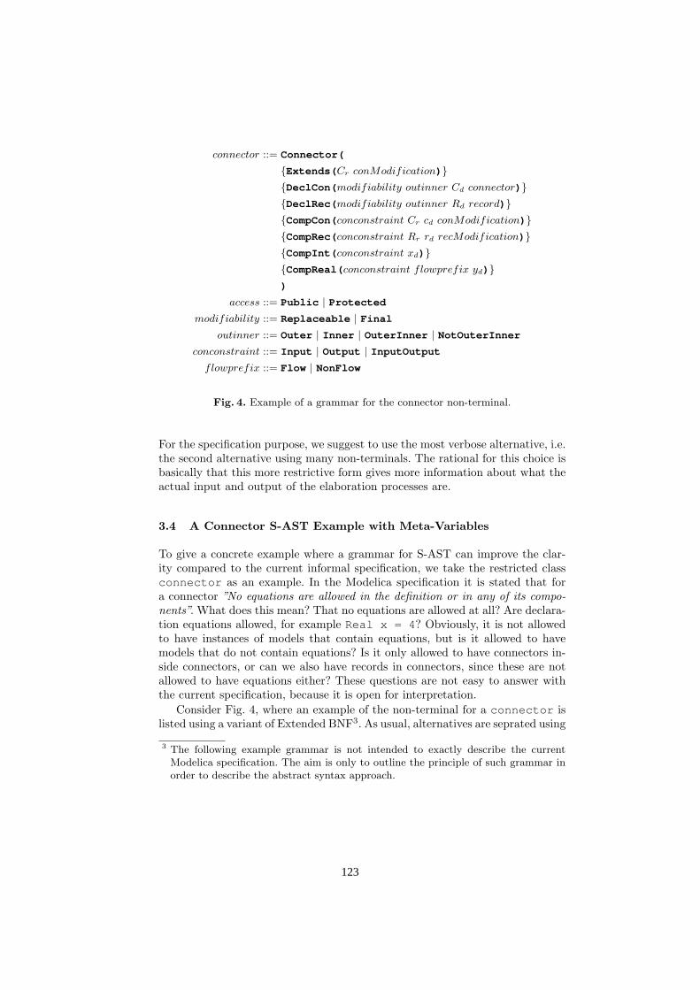
connector ::= Connector(

Extends( Cr conModification) DeclCon( modifiability outinner Cd connector)DeclRec( modifiability outinner Rd record)CompCon(conconstraint Cr cd conModification)CompRec(conconstraint Rr rd recModification)CompInt( conconstraint xd)CompReal( conconstraint flowprefix yd))

access ::= Public | Protected

modifiability ::= Replaceable | Final

outinner ::= Outer | Inner | OuterInner | NotOuterInner

conconstraint ::= Input | Output | InputOutput

flowprefix ::= Flow | NonFlow

Fig. 4. Example of a grammar for the connector non-terminal.

For the specification purpose, we suggest to use the most verbose alternative, i.e.the second alternative using many non-terminals. The rational for this choice isbasically that this more restrictive form gives more information about what theactual input and output of the elaboration processes are.

3.4 A Connector S-AST Example with Meta-Variables

To give a concrete example where a grammar for S-AST can improve the clar-ity compared to the current informal specification, we take the restricted classconnector as an example. In the Modelica specification it is stated that fora connector ”No equations are allowed in the definition or in any of its compo-nents”. What does this mean? That no equations are allowed at all? Are declara-tion equations allowed, for example Real x = 4? Obviously, it is not allowedto have instances of models that contain equations, but is it allowed to havemodels that do not contain equations? Is it only allowed to have connectors in-side connectors, or can we also have records in connectors, since these are notallowed to have equations either? These questions are not easy to answer withthe current specification, because it is open for interpretation.

Consider Fig. 4, where an example of the non-terminal for a connector islisted using a variant of Extended BNF3. As usual, alternatives are seprated using

3 The following example grammar is not intended to exactly describe the currentModelica specification. The aim is only to outline the principle of such grammar inorder to describe the abstract syntax approach.

123

the ’|’ symbol, and curly brackets (. . . ) denote that the enclosing elements canbe repeated zero or more times.

The grammar is extended with a more abstract notation of metavariables,which range over names or identifiers. Metavariables Cd and Rd range over iden-tifiers declaring a new connector respectively record; Cr and Rr range over con-nector and record names referencing an already declared connector or record.Metavariables cd, rd, xd, and yd range over component identifiers having thetype of connector, record, Integer, and Real. All bold strings denote a node inthe AST. If the AST is given in a concrete textual representation, these keywordsare used when performing a pre-order traversal of the tree.

In the example, connector can hold zero or many extends nodes, referencingthe meta-variable Cr, denoting all names that reference a declared connector.Hence, using this meta-variable notation, this rule states that a connector is onlyallowed to inherit from another connector.

Furthermore, the example shows that a connector is allowed to have twokinds of local classes: Connector and Record (nodes DeclCon and DeclRec ).CompConand CompRec state that a connector can have both connector andrecord components.

For each of the different kinds of elements, it is stated exactly which prefixesthat are allowed. This description is more restrictive than the concrete syntax,which basically allows any prefix. In the current specification these restrictionsare stated in natural languages, spread out over the specification. For example,on one page it is stated ”Variables declared with the flow type prefix shall be asubtype of Real”. Such a text is superfluous when the grammar for S-AST isspecified (note that flowprefix is only available in the CompReal node).

3.5 What can and should be specified by the abstract syntax?

In the previous sections we have briefly outlined how an abstract syntax grammarcan specify the structure of input and output of a transformation, but also as amethod for specifying context-dependent information about rejection of illegalmodels. The question then arise: what should be specified using this grammarapproach, and what should be addressed with other semantic rules?

The proposed grammar approach with meta-variables is declarative in thesense that it does not state information about how the rejecting rules shouldbe implemented. Hence, it is less formal compared to e.g. a formal type system.However, it is still more precise than giving the rules using natural languages.

We believe that as long as the alternative semantic description is using nat-ural languages, the abstract syntax approach can both be easier to understandand less ambiguous. Furthermore, if it can be complemented with aspects whichare more precisely described, e.g. the lookup-process, it can clarify the specifi-cation even more. However, several parts of the rejection aspect, e.g. subtypingrules, cannot be described with the abstract syntax grammar. The other aspectof transformation semantics can of course not be specified with this approach.

The concept is still at a very early stage, and further investigations need tobe performed, to see if this approach can cover the current Modelica language.

124

4 Conclusion

In this paper we have given an overview of different aspects of defining a modelinglanguage; using the Modelica language’s syntax and semantics.

Furthermore, we have argued that an approach which uses abstract syntaxto describe both the input to Modelica’s elaboration process (S-AST) as well asits output (HDAE-AST) can both clarify the transformation process as well asthe rejection of invalid models. Furthermore, while developing the language, thisapproach promotes the focus on semantic issues, to avoid getting trapped in thecommon syntax pitfall.

The obvious next step for future work would be to design and implement theS-AST and HDAE-AST, and to verify that the ASTs meets most of the currentcode base publicly available.

We have described this as an evolutionary approach, which is intended to bepractical in the short-term. However, in the long term, we still think that it isimportant that a formal semantics is given for the Modelica language.

Acknowledgments

We would like to thank the anonymous reviewers for their suggestions and JohanAkesson and Asa Broman for useful comments and feedback.

This research work was funded by CUGS (the Swedish National GraduateSchool in Computer Science), by SSF under the VISIMOD project, and by Vin-nova under the NETPROG Safe and Secure Modeling and Simulation on theGRID project.

References

1. Alfred V. Aho, Monica S. Lam, Ravi Sethi, and Jeffrey D. Ullman. Compilers:Principles, Techniques, and Tools. Addison-Wesley, 2nd edition.

2. David Broman, Peter Fritzson, and Sebastien Furic. Types in the Modelica Lan-guage. In Proceedings of the Fifth International Modelica Conference, Vienna,Austria, 2006.

3. David Broman, Kaj Nystrom, and Peter Fritzson. Determining Over- and Under-Constrained Systems of Equations using Structural Constraint Delta. In Pro-ceedings of the Fifth International Conference on Generative Programming andComponent Engineering (GPCE’06), Portland, Oregon, USA, 2006. ACM Press.

4. Dynasim. Dymola - Dynamic Modeling Laboratory with Modelica (Dynasim AB).http://www.dynasim.se/ [Last accessed: 22 June 2007].

5. Christoph Nytsch-Geusen et. al. MOSILAB: Development of a Modelica basedgeneric simulation tool supporting model structural dynamics. In Proceedings ofthe 4th International Modelica Conference, Hamburg, Germany, 2005.

6. Peter Fritzson. Developing Efficient Language Implementations from Structuraland Natural Semantics - Draft Version 0.97. 2006. Book draft available from:http://www.ida.liu.se/~pelab/rml/ .

125

7. Peter Fritzson, Peter Aronsson, Adrian Pop, Hakan Lundvall, Kaj Nystrom, LevonSaldamli, David Broman, and Anders Sandholm. OpenModelica - A Free Open-Source Environment for System Modeling, Simulation, and Teaching. In IEEEInternational Symposium on Computer-Aided Control Systems Design, Munich,Germany, 2006.

8. Peter Fritzson, Adrian Pop, and Peter Aronsson. Towards Comprehensive Meta-Modeling and Meta-Programming Capabilities in Modelica. In Proceedings of the4th International Modelica Conference, Hamburg, Germany, 2005.

9. James Gosling, Bill Joy, Guy Steele, and Gilad Bracha. The Java Language Spec-ification, 3rd Edition. Prentice Hall, 2005.

10. Atsushi Igarashi, Benjamin C. Pierce, and Philip Wadler. Featherweight Java:a minimal core calculus for Java and GJ. ACM Trans. Program. Lang. Syst.,23(3):396–450, 2001.

11. ISO/IEC. ISO/ IEC 14882 : Programming language C++. ANSI, New York, USA,1998.

12. ITI. SimulationX. http://www.iti.de/ [Last accessed: 22 June 2007].13. Gilles Kahn. Natural semantics. In 4th Annual Symposium on Theoretical Aspects

of Computer Sciences on STACS 87, pages 22–39, London, UK, 1987. Springer-Verlag.

14. David Kagedal. A Natural Semantics specification for the equation-based modelinglanguge Modelica. Master’s thesis, Linkoping University, 1998.

15. David Kagedal and Peter Fritzson. Generating a Modelica Compiler from Nat-ural Semantics Specifications. In Proceedings of the Summer Computer SimulationConference, 1998.

16. MathCore. MathModelica System Designer: Model based design ofmulti-engineering systems. http://www.mathcore.com/products/mathmodelica/ [Last accessed: 8 March 2007].

17. Jakob Mauss. Modelica Instance Creation. In Proceedings of the 4th InternationalModelica Conference, Hamburg, Germany, 2005.

18. Robin Milner, Mads Tofte, Robert Harper, and David MacQuee. The Definitionof Standard ML - Revised. The MIT Press, 1997.

19. Modelica Association. Modelica - A Unified Object-Oriented Language for PhysicalSystems Modeling - Version 1, September 1997. Available from: http://www.modelica.org .

20. Modelica Association. Modelica - A Unified Object-Oriented Language for PhysicalSystems Modeling - Language Specification Version 2.2, February 2005. Availablefrom: http://www.modelica.org .

21. OpenModelica. Project. http://www.ida.liu.se/~pelab/modelica/OpenModelica.html [Last accessed: 22 June 2007].

22. Mikael Pettersson. Compiling Natural Semantics. PhD thesis, Linkoping Univer-sity, 1995.

23. Linda R. Petzold. A Description of DASSL: A Differential/Algebraic System Solver.In IMACS Trans. on Scientific Comp., 10th IMACS World Congress on SystemsSimulation and Scientific Comp., Montreal, Canada, 1982.

24. Benjamin C. Pierce. Types and Programming Languages. The MIT Press, 2002.25. Gordon D. Plotkin. A Structural Approach to Operational Semantics. Technical

report, Dept. of Computer Science, University of Aarhus, 1981.26. Andrew K. Wright and Matthias Felleisen. A Syntactic Approach to Type Sound-

ness. Information and Computation, 115(1):38–94, 1994.

126

Physical Modeling with ModelVision, a DAE Simulator

with Features for Hybrid Automata

Abstract for short talk

Yuri Senichenkov1, Felix Breitenecker2, Günther Zauner2 1Technical University St.Petersburg, Dept. for Distributed Computing and Networking

2Vienna University of Technology, Wiedner Hauptstr. 8-10, 1040 Vienna, Austria

senyb@dcn.infos.ru

Abstract. This contribution presents the modeling capabilities of the fully

hybrid simulator ModelVision. Development of ModelVision started in the

1990ies, in autumn 2007 an English version is to be released. Basis of

ModelVision are hybrid statecharts, allowing any parallel, serial, and

conditional combination of continuous models, described by DAEs. State

models itself are objects to be instantiated in various kinds, so that structural-

dynamic systems of any kind can be modeled. DAE modeling is supported by

an editor capable of editing mathematical formula.

Project representation can be done in visual and textual form, respectively. These representations can

be restored from each other.

A subset of UML for Real Time was chosen and extended to incorporate continuous behavior. The

modeling language implemented in our tool supports two types of UML diagrams: collaboration diagrams

and state chart (state machine) diagrams with some changes. In collaboration diagrams we have added

unidirectional continuous connections between objects (capsules in UML-RT) and the corresponding

interface elements – input and output variables. UML state charts are made hybrid: a system of algebraic-

differential equations over variables (interface or object’s internal ones) can be associated with each

simple or composite state. To make such an UML-based model fully executable we have taken Java as a

reasonably high-level language for defining data types and data transformation.

As an example we consider an airplane ejection process. This model has a hybrid structure. The

equations and states can be represented in our notation like in the lower left figure.

The catapulting will start when external signal ‘Eject’ occurs. The first state

of catapulting is track moving with fixed velocity. The second state is free flight

which will start after an arm-chair has left airplane and will stop either by

parachute opening after delay TauP, or by arm-

chair and airplane collision and destruction. The

B-Chart of the device is shown in the left figure.

The solution is calculated following the hybrid

event calendar in the right figure.

Users are recommended to construct a

Behavior-Chart. Thus, the solved system has

fixed structure and smooth right-hand sides.

Three Equation Solvers may be suggested,

which are ODE-solver, DAE-solver and AE-solver. By Equation Solver we

mean a heuristic algorithm that chooses the simplest numerical software for solving a problem with user

prescribed tolerance. All our Solvers are based on numerical software available in the Web, namely

ODEPACK, Hairer, Norsett, Wanner and Hairer, Wanner collection, DASSL and some others programs.

127

An Approach to the Calibration of Modelica

Models

Miguel A. Rubio, Alfonso Urquia, and Sebastian Dormido

Departamento de Informatica y Automatica, UNEDJuan del Rosal 16, 28040 Madrid, Spain

marubio,aurquia,sdormido@dia.uned.es

Abstract. An approach to the calibration of Modelica models using ge-netic algorithms (GA) is presented. The functions required to performthe model calibration have been programmed in the Modelica languageand structured in a Modelica library, called GAPILib. This Modelica li-brary is intended for parameter estimation in any Modelica model, sup-porting simple-objective optimization. Model calibration with GAPILibdoes not require to perform model modifications. During the algorithmrun, the user can interactively change the value of the GA parameters.In addition, GAPILib supports parameter sensitivity analysis, and it iswell suited for parallel computing. GAPILib is a free library (availableon http://www.euclides.dia.uned.es/GAPILib) that can be easily used,modified and extended.The design, implementation and use of GAPILib are discussed in thismanuscript. Its use is illustrated by means of a case study: the estima-tion of electrochemical parameters in fuel cell models, which have beencomposed using FuelCellLib Modelica library.

1 Introduction

Genetic algorithms (GA) are used for model parameter estimation from experi-mental data. The main advantage of this technique lies in its robustness and sim-plicity. GA can be successfully applied for finding solutions in high-dimensionalsearch spaces. The search range of the parameters can be changed during thealgorithm run [1]. In addition, parallel implementations of genetic algorithms,intended to reduce the computation time, have been developed.

The use of GA for parameter estimation in Modelica models has been pre-viously proposed by [2]. However, those authors implemented and ran the GAusing Matlab/Simulink. As a consequence, those author’s approach requires thecombined use of Modelica/Dymola and Matlab/Simulink.

The lack of a freely-available Modelica library implementing GA, suited forparameter estimation in Modelica models, has motivated the implementation ofthe GAPILib library [3]. Two key advantages of GAPILib are its simplicity of useand generality: it can be applied for parameter estimation in any Modelica model,without needing to modify the model. The GAPILib library is freely availableand can be downloaded from http://www.euclides.dia.uned.es/GAPILib

129

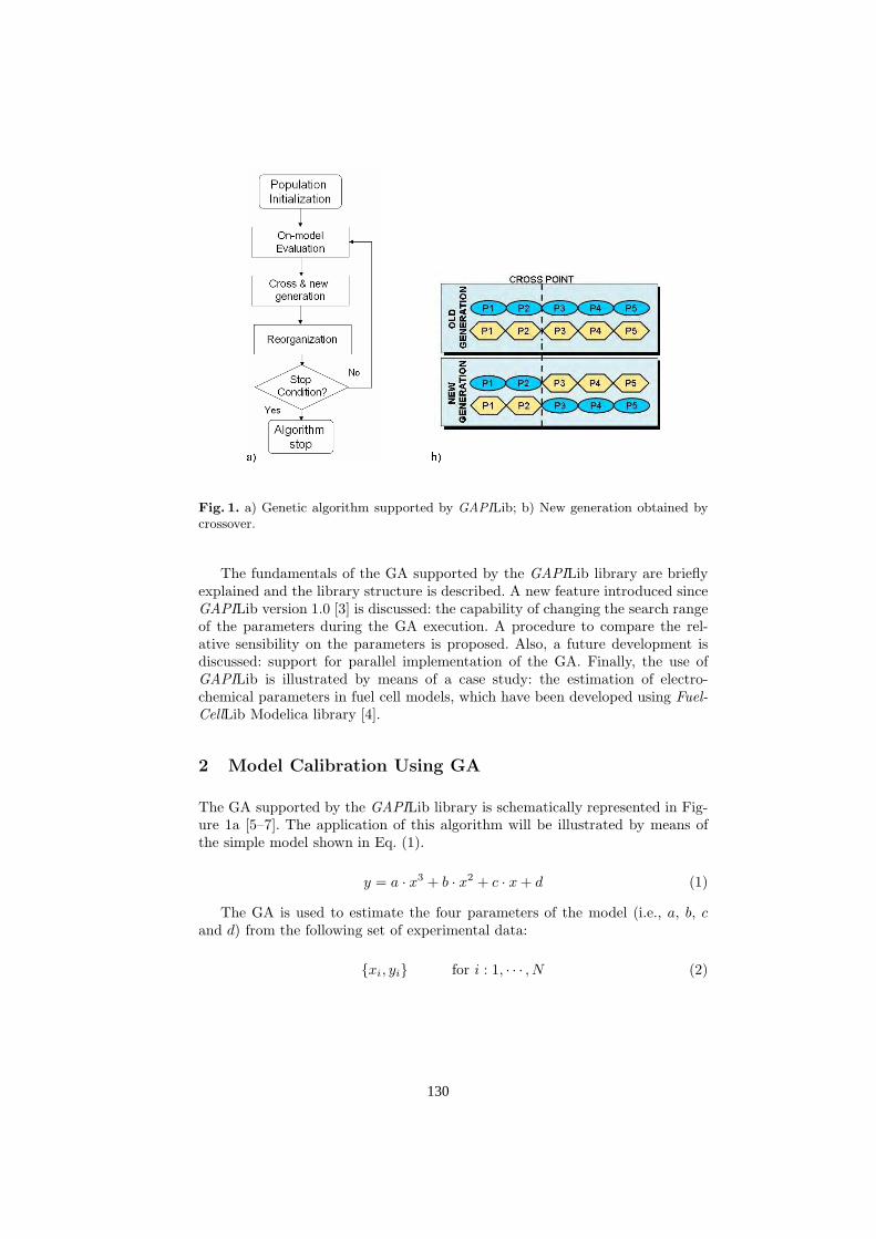
Fig. 1. a) Genetic algorithm supported by GAPILib; b) New generation obtained bycrossover.

The fundamentals of the GA supported by the GAPILib library are brieflyexplained and the library structure is described. A new feature introduced sinceGAPILib version 1.0 [3] is discussed: the capability of changing the search rangeof the parameters during the GA execution. A procedure to compare the rel-ative sensibility on the parameters is proposed. Also, a future development isdiscussed: support for parallel implementation of the GA. Finally, the use ofGAPILib is illustrated by means of a case study: the estimation of electro-chemical parameters in fuel cell models, which have been developed using Fuel-CellLib Modelica library [4].

2 Model Calibration Using GA

The GA supported by the GAPILib library is schematically represented in Fig-ure 1a [5–7]. The application of this algorithm will be illustrated by means ofthe simple model shown in Eq. (1).

y = a · x3 + b · x2 + c · x + d (1)

The GA is used to estimate the four parameters of the model (i.e., a, b, c

and d) from the following set of experimental data:

xi, yi for i : 1, · · · , N (2)

130

The GA starts with an initial population, composed of NPOPULATION in-dividuals, which are randomly selected from the search space. Each individualof the population is formed by a group of chromosomes, which represents a so-lution to the problem. In case of the model shown in Eq. (1), each individualconsists of a specific value of the parameters a, b, c and d. The j-th individual ofthe population is Ij = aj , bj , cj , dj. These initial values are randomly selectedfrom the parameter search ranges.

Each individual of this initial population is evaluated by using a cost function.This function is used to calculate the validity of the population members. Thecost function, evaluated for the j-th individual of the population, is the following:

fj =

N∑

i:1

(yi − yi,j)2

(3)

where

yi,j = ajx3

i + bjx2

i + cjxi + dj (4)

The population members (i.e., Ij, with j = 1, . . ., NPOPULATION ) aresorted according to this criterion (i.e., the smaller fj , the better). The sortedindividuals can be represented as I(1), I(2), . . . , I(NPOPULATION ), where I(1)is the best one (i.e., that with the smallest cost function).

– The NELITISM best individuals (i.e., I(1), I(2), . . . , I(NELITISM)) pass un-changed to the following generation.

– The next NPARENTS individuals (i.e., I(NELITISM + 1), I(NELITISM +2), . . . , I(NELITISM+NPARENTS)) go through the crossover (see Figure 1b)and mutation processes.

– The remaining individuals of the population (i.e., I(NELITISM+NPARENTS+1), . . . , I(NPOPULATION )) are discarded.

The new generation is composed of the NELITISM best individuals of theprevious generation, the NPARENTS individuals obtained from the crossoverand mutation processes, and NPOPULATION − NELITISM − NPARENTS newmembers, which are randomly selected from the search space. The individualsof this new generation are evaluated using the cost function, sorted, etc. Thealgorithm steps are repeated until the stop condition is reached (see Figure 1a).

The GA supported by GAPILib includes several processes intended to im-prove the algorithm performance, such as elitism and mutation.

– Elitism ensures that the most valid individuals pass on to the next genera-tion without being altered by genetic operators. It guarantees that the bestsolution is never lost from one generation to the next.

– Mutation introduces random changes on the individuals, maintaining geneticdiversity from one generation of the population of chromosomes to the next.The purpose of mutation is to allow the algorithm to avoid local minima.

131

Fig. 2. GAPILib library: a) Functions; b) Script files with the function calls signaled.

3 GAPILIB Architecture

GAPILib has been implemented by combining the use of the scripting Model-ica language and the use of functions written in the Modelica language. Thefunctions, which are stored within the GAPILib.Basics package, are listed inFigure 2a. A detailed description of these functions can be found in [3].

GAPILib contains a set of script files, written in scripting Modelica language(.mos files in Figure 2b), that implement the GA. The GA execution is startedby running the script file GAPILib.mos (see Figure 2b). This file contains thesentences required to execute the script files that set the GA initial conditions:

– GAPILib INI.mos carries out the initialization of the GA parameters, includ-ing the number of individuals of the population (NPOPULATION ), elitistindividuals (NELITISM), parents (NPARENTS) and cross points (see Fig-ure 1b). Also, the mutation probability, the stop condition of the GA, thepath of the file containing the experimental data, the Modelica model, thestart and stop times for the Modelica model simulation, etc. are set in thisscript file.

– GAPILib POPINIT.mos randomly generates the initial population.– GAPILib CROSSPOINT.mos randomly sets the initial value of the cross

point, which is used in the crossover process (see Figure 1b).

The Ram Gen ARENA function, which is a pseudo-random number genera-tor, is called by POPINIT and CROSSPOINT script files.

Next, GAPILib.mos executes a loop until the GA stop condition is satisfied.The stop condition shown in Figure 2b is of the type: “N Cycle generations havebeen obtained”. Other stop conditions are possible, e.g., “the calculated fitness

132

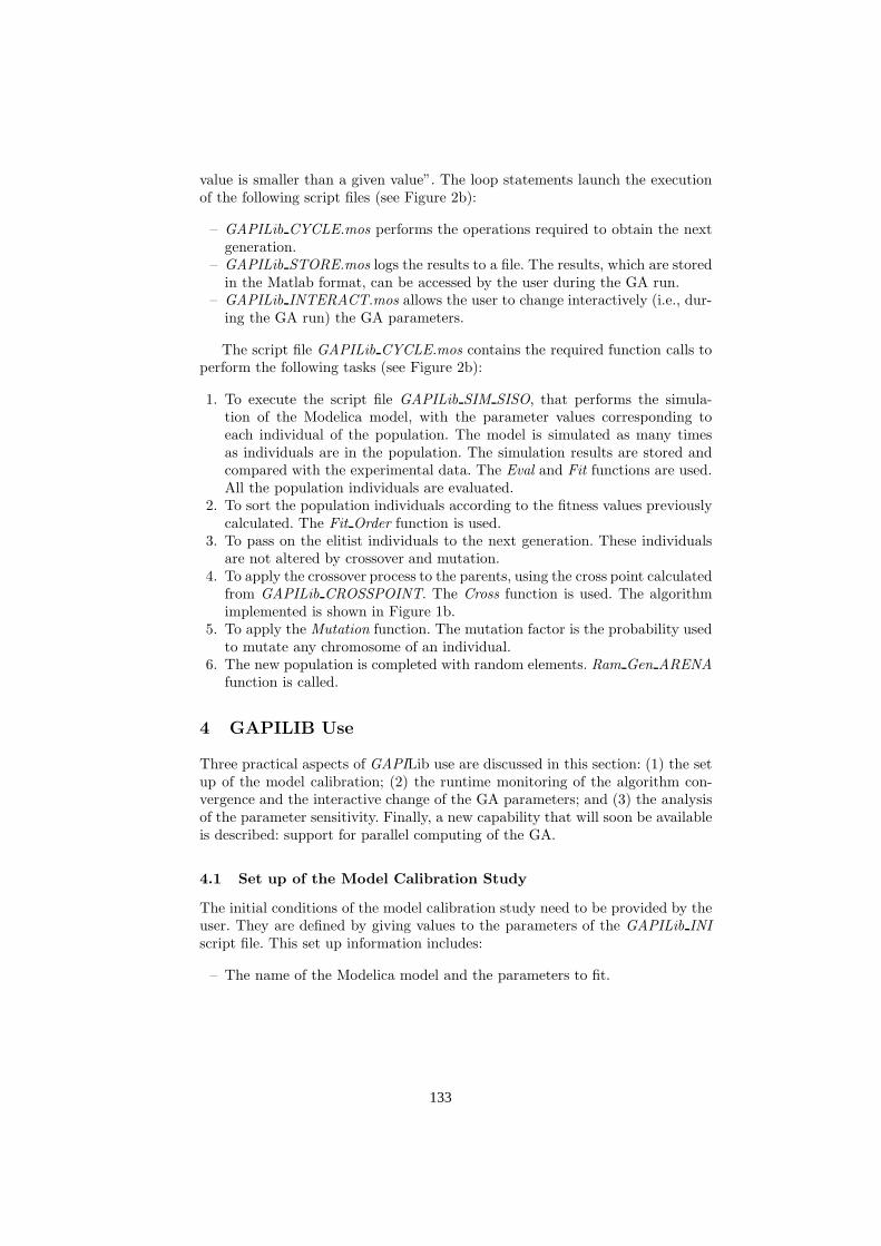
value is smaller than a given value”. The loop statements launch the executionof the following script files (see Figure 2b):

– GAPILib CYCLE.mos performs the operations required to obtain the nextgeneration.

– GAPILib STORE.mos logs the results to a file. The results, which are storedin the Matlab format, can be accessed by the user during the GA run.

– GAPILib INTERACT.mos allows the user to change interactively (i.e., dur-ing the GA run) the GA parameters.

The script file GAPILib CYCLE.mos contains the required function calls toperform the following tasks (see Figure 2b):

1. To execute the script file GAPILib SIM SISO, that performs the simula-tion of the Modelica model, with the parameter values corresponding toeach individual of the population. The model is simulated as many timesas individuals are in the population. The simulation results are stored andcompared with the experimental data. The Eval and Fit functions are used.All the population individuals are evaluated.

2. To sort the population individuals according to the fitness values previouslycalculated. The Fit Order function is used.

3. To pass on the elitist individuals to the next generation. These individualsare not altered by crossover and mutation.

4. To apply the crossover process to the parents, using the cross point calculatedfrom GAPILib CROSSPOINT. The Cross function is used. The algorithmimplemented is shown in Figure 1b.

5. To apply the Mutation function. The mutation factor is the probability usedto mutate any chromosome of an individual.

6. The new population is completed with random elements. Ram Gen ARENAfunction is called.

4 GAPILIB Use

Three practical aspects of GAPILib use are discussed in this section: (1) the setup of the model calibration; (2) the runtime monitoring of the algorithm con-vergence and the interactive change of the GA parameters; and (3) the analysisof the parameter sensitivity. Finally, a new capability that will soon be availableis described: support for parallel computing of the GA.

4.1 Set up of the Model Calibration Study

The initial conditions of the model calibration study need to be provided by theuser. They are defined by giving values to the parameters of the GAPILib INIscript file. This set up information includes:

– The name of the Modelica model and the parameters to fit.

133

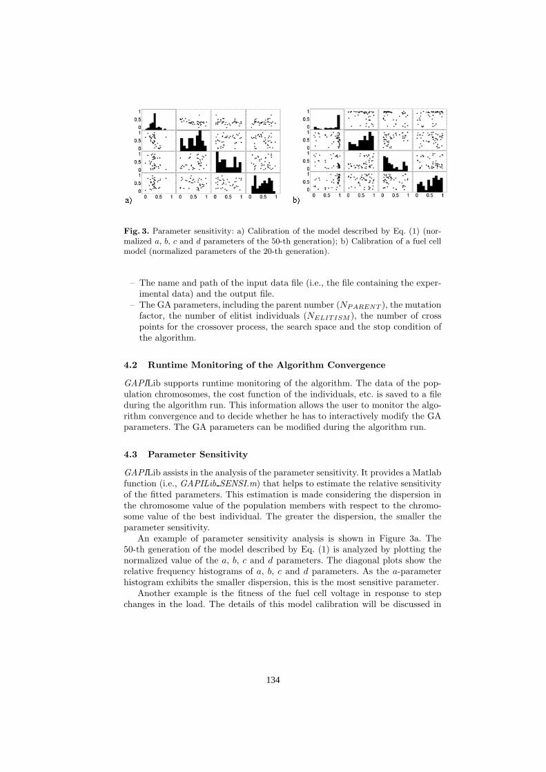
Fig. 3. Parameter sensitivity: a) Calibration of the model described by Eq. (1) (nor-malized a, b, c and d parameters of the 50-th generation); b) Calibration of a fuel cellmodel (normalized parameters of the 20-th generation).

– The name and path of the input data file (i.e., the file containing the exper-imental data) and the output file.

– The GA parameters, including the parent number (NPARENT ), the mutationfactor, the number of elitist individuals (NELITISM), the number of crosspoints for the crossover process, the search space and the stop condition ofthe algorithm.

4.2 Runtime Monitoring of the Algorithm Convergence

GAPILib supports runtime monitoring of the algorithm. The data of the pop-ulation chromosomes, the cost function of the individuals, etc. is saved to a fileduring the algorithm run. This information allows the user to monitor the algo-rithm convergence and to decide whether he has to interactively modify the GAparameters. The GA parameters can be modified during the algorithm run.

4.3 Parameter Sensitivity

GAPILib assists in the analysis of the parameter sensitivity. It provides a Matlabfunction (i.e., GAPILib SENSI.m) that helps to estimate the relative sensitivityof the fitted parameters. This estimation is made considering the dispersion inthe chromosome value of the population members with respect to the chromo-some value of the best individual. The greater the dispersion, the smaller theparameter sensitivity.

An example of parameter sensitivity analysis is shown in Figure 3a. The50-th generation of the model described by Eq. (1) is analyzed by plotting thenormalized value of the a, b, c and d parameters. The diagonal plots show therelative frequency histograms of a, b, c and d parameters. As the a-parameterhistogram exhibits the smaller dispersion, this is the most sensitive parameter.

Another example is the fitness of the fuel cell voltage in response to stepchanges in the load. The details of this model calibration will be discussed in

134

Fig. 4. Parallel computing of the GA using GAPILib.

Section 5. The goal is to fit the four parameters shown in Table 2. The relativefrequency histograms of the 20-th generation chromosomes are plotted in Fig-ure 3b. The first and third parameters (i.e., Rinf and Cdl) exhibit less dispersionthan the other two parameters (i.e., Rsup and ks). As a consequence, Rinf andCdl are more sensitive than Rsup and ks.

4.4 Parallel Computing of the GA

Parallel computing allows reducing the time required to complete the modelcalibration study. Next version of GAPILib will support the parallelization ofthe GA. The architecture is shown in Figure 4. GAPILib needs to be installedin all the computers, which have to be connected (e.g., using TCP/IP).

Initially, the user starts the GAPILib MASTER script file in the mastercomputer. This script file sends random seeds to the other computers, in orderto guarantee that the sequences of pseudo random numbers used in the differentcomputers are independent.

Then, the GA is run independently in each computer during certain numberof generations (N Cycle matrix). Periodically, the chromosomes of the best in-dividuals obtained in each computer are saved in a shared folder (see Figure 4)and they are included in the next generation of all the computers.

5 Case Study: Calibration of Fuel Cell Models using

GAPILib

GAPILib has been successfully applied to the estimation of electrochemical pa-rameters in fuel cell models composed by using FuelCellLib Modelica library [4].The obtained models can be used to simulate the steady-state and the dynamic

135

Fig. 5. Experimental (–), simulated using FuelCellLib (- -): a) Fuel cell polarizationcurve; b) Fuel cell voltage in response to step changes in the load, Voltage [V] vs. Time[s].

behavior of the fuel cells along their complete range of operation [8–10]. Threemodel calibrations have been performed, in order to fit the model to:

1. The experimental polarization curve (I-V) of a fuel cell.2. The experimental data of the fuel cell voltage obtained in response to step

changes in the load.3. The experimental data of the water long-term effect. The fitted model re-

produces:(a) The slow voltage rise due to the membrane hydrate.(b) The voltage fall due to the water flooding of the cathode.

5.1 Fitness of the Polarization Curve

In order to obtain the polarization curve, the model has to be simulated, for eachof the operation points composing the curve, until the steady-state is reached.The parameters estimated and the obtained values are shown in Table 1. Onecross point was used. The fitness function was defined as the sum of the quadraticdifferences between the experimental and the simulated values of the variable.

The GA parameters were set to the following values: the stop condition issatisfied after 5000 generations; the population was composed of 100 individu-als; the mutation factor was 0.25; NPARENT = 70; and NELITISM = 1. Theexperimental data of the fuel cell polarization curve and the simulation resultsof the calibrated model are shown in Figure 5a.

136

Table 1. Model parameters and their fitted values.

Parameter Value Unit

A Tafel Slope 0.0390 V

In Internal current density 1.4 · 10−3A · cm−2

I0 Exchange current density 1.5856 · 10−6A · cm−2

B Mass Transfer slope 0.0918 V

R Internal specific resistance 7.2860 · 10−4Ω · cm−2

Ilim Limiting internal current density 0.2265 A · cm−2

Table 2. Model parameters and their fitted values.

Parameter Value Unit

Rinf Low value of the load 0.03315 Ω · m−2

Rsup High value of the load 5.1 Ω · m−2

Cdl Double layer capacitance 10.12 F · m−2

ks Electrical conductivity of the solid 0.01 S · m−1

5.2 Fitness of the Fuel Cell Voltage in Response to Step Changes in

the Load

GAPILib is used to estimate the values of the four parameters shown in Table2. The GA parameters are set to the following values: the stop condition issatisfied after 200 generations; the population contains 150 individuals; a factorof mutation of 0.25 was applied; NPARENT = 100; and NELITISM = 1. Theexperimental data of the fuel cell response to step changes in the load and thesimulation results of the calibrated model are shown in Figure 5b.

5.3 Fitness of the Long Term Effect of Water on the Fuel Cell

Voltage with Constant Resistance Load

The fuel cell model was modified in order to reproduce the variation of themembrane conductivity. The parameters used to fit the model are shown in Table3. The GA parameters were set to the following values: the stop condition wassatisfied after 700 generations; the population was composed of 70 individuals;a factor of mutation of 0.15 was applied; NPARENT = 50; and NELITISM = 1.The experimental data of the cathode flooding process and the simulation resultsof the calibrated model are shown in Figure 6.

137

Table 3. Model parameters and their fitted values.

Parameter Value Unit

da(Act) Width of active layer 6 · 10−8m

εg Volume fraction of pore 0.05

D12 Binary diffusion coefficient 5 · 10−9m

2 · s−1

da(Mem) Width of membrane layer 1.6 · 10−5m

Rmem Resistance of membrane layer 1.42 · 10−3Ω · m−2

Fig. 6. Experimental (–), simulated using FuelCellLib (- -): long-term effect of thewater with a constant load applied, Voltage [V] vs. Time [s].

6 Conclusions

The design, implementation and use of GAPILib has been discussed. The GAPILiblibrary is an effective tool for parameter identification in Modelica models usingGA. It is completely written in the Modelica language, which facilitates its use,modification and extension. GAPILib can be used for parameter identificationin any Modelica model and the estimation process does not require to performmodel modifications. GAPILib has been successfully applied to the estimationof electrochemical parameters in fuel cell models, which have been composed byusing FuelCellLib library.

Acknowledgements

This work has been supported by the Spanish CICYT, under DPI2004-01804grant, and by the IV PRICIT (Plan Regional de Ciencia y Tecnologia de laComunidad de Madrid, 2005-2008), under S-0505/DPI/0391 grant.

The fuel cell experimental data used in this work has been obtained in theLaboratory of Renewable Energy of the IAI-CSIC in Madrid (Spain).

138

References

1. Stuckman, B., Evans, G., Mollaghasemi, M.: Comparison of Global Search Meth-ods for Design Optimization Using Simulation. In: Proceedings of 1991 WinterSimulation Conference, 1991, pp. 937–944.

2. Hongesombut, K., Mitani, Y., Tsuji, K.: An Incorporated Use of Genetic Algorithmand a Modelica Library for Simultaneous Tuning of Power System Stabilizers. In:Proceedings of the 2nd International Modelica Conference, 2002, pp. 89–98.

3. Rubio, M.A., Urquia, A., Gonzalez, L., Guinea, D., Dormido, S.: GAPILib - AModelica Library for Model Parameter Identification Using Genetic Algorithms,In: Proceedings of 5th International Modelica Conference, 2006, pp. 335–342.

4. Rubio, M.A., Urquia, A., Gonzalez, L., Guinea, D., Dormido, S.: FuelCellLib - AModelica Library for Modeling of Fuel Cells. In: Proceedings of the 4th Interna-tional Modelica Conference, 2005, pp. 75–82.

5. Goldberg, D.E.: Genetic Algorithms in Search, Optimization and Machine Learn-ing, Kluwer Academic Publishers, Boston, MA, 1989.

6. Holland, J.H.:Adaptation in Natural and Artificial Systems, University of MichiganPress, Ann Arbor, 1975.

7. Mitchell, M.: An Introduction to Genetic Algorithms, MIT Press, Cambridge, MA.,1996.

8. Larminie, J., Dicks, A.: Fuel Cell Systems Explained, Wiley, 2000.9. Bevers, D., Wohr, M., Yasuda, K., Oguro, K.: Simulation of Polymer Electrolyte

Fuel Cell Electrode. J. Appl. Electrochem, 27 (1997).10. Broka, K., Ekdunge, P.: Modelling the PEM Fuel Cell Cathode, J. Appl. Elec-

trochem. 27 (1997).

139

Dynamic Optimization of Modelica Models –

Language Extensions and Tools

Johan Akesson

Department of Automatic ControlFaculty of Engineering

Lund UniversitySweden

jakesson@control.lth.se

Abstract. The Modelica language is currently gaining increased inter-est, both in industry and in academia. Modelica is an object-oriented,general purpose modeling language, targeted at modeling of complexphysical systems. While the main usage of models developed in Mod-elica is simulation, several other usages emerge. Examples of such us-ages are dynamic optimization, model reduction, calibration, verificationand code generation for embedded systems. This paper reports the cur-rent status of the JModelica project, in which an extensible, Java-basedModelica compiler is being developed. In addition, an extension of theModelica language directed towards dynamic optimization, Optimica, isdiscussed.

1 Introduction

High-level modeling languages are receiving increased industrial and academicinterest within several domains, such as chemical engineering, thermo-fluid sys-tems and automotive systems. One such modeling language is Modelica, [8].Modelica is an open language, specifically targeted at multi-domain modelingand model re-use. Key features of Modelica include object oriented modeling,declarative equation-based modeling, and a component model enabling acausalconnections of submodels, as well as support for hybrid/discrete behaviour.These features have proven very applicable to large-scale modeling problemsin various fields.

While there exist very efficient software tools for simulation of Modelicamodels, tool support for static and dynamic optimization is generally weak. Fur-thermore, specification of optimization problems is not supported by Modelica.Since Modelica models represent an increasingly important asset for many com-panies, it is of interest to investigate how Modelica models can be used also foroptimization.

This contribution gives an overview of a project, entitled JModelica, tar-geted at i) defining an extension of Modelica, Optimica, which enables high-level formulation of optimization problems, ii) developing prototype tools fortranslating a Modelica model and a complementary Optimica description into a

141

representation suited for numerical algorithms, and iii) performing case studiesdemonstrating the potential of the concept.

The project integrates dynamic modeling and optimization with computerscience and numerical algorithms. One of the main benefits of the suggested ap-proach is that the high-level descriptions are automatically translated into anintermediate representation by the compiler front-end. This intermediate rep-resentation can then be further translated to interface with different numericalalgorithms. The user is therefore relieved from the burden of managing the oftencumbersome API:s of numerical algorithms. The flexibility of the architecturealso enables the user to select the algorithm most suitable for the problem athand.

2 Software Tools

In order to demonstrate the proposed concept, prototype software tools are beingdeveloped. In essence, the task of the software is to read the Modelica and Opti-mica source code and then translate, automatically, the model and optimizationdescriptions into a format which can be used by a numerical algorithm. The coreof the software is a compiler front-end, referred to as the JModelica compiler,which translates a subset of Modelica into a flat model description. In addition,an extended front-end, based on the JModelica compiler, supporting a first pro-totype of the Optimica extension has been developed. The extended compiler isreferred to as the Optimica compiler. In addition, a back-end for generation ofefficient code for dynamic optimization has been developed.

2.1 Development Environment

The JModelica compiler is developed using the Java-based compiler constructiontool JastAdd, [7]. JastAdd is a development environment targeted at implemen-tation of the semantics of computer programming languages, and has also beenexplicitly designed with modular and extensible compiler construction in mind.The core concepts used in JastAdd are object orientation, static aspect orienta-tion, and reference attributed grammars [6].

The JastAdd system is based on an object oriented specification of an ab-stract grammar (AG), from which standard Java classes are generated. Seman-tic behaviour is added in aspects, which are useful for organizing cross-cuttingbehaviour. It is natural to structure the implementation of different semanticfunctions, such as name analysis (the task of binding identifiers to declarations)and type analysis (e.g. computation of the types of expressions), into separatemodules. However, since the implementation of, for example, name analysis, typ-ically affects a large number of classes, the object-oriented paradigm does notinherently offer support for this kind of modularization. In JastAdd, this prob-lem is overcome by allowing definition of behaviour, in the form of inter-typedeclarations, in separate aspects, which are then woven into the AG classes. The

142

resulting classes contain only Java code, and can be compiled by a standard Javacompiler.

The choice of JastAdd is natural in this project, since its main focus isextensions of the Modelica language. In particular, the methodology adoptedby JastAdd enables the implementations of the core language compiler and theextensions to be separated. It is then possible to build the core compiler alone,or with one or more extensions. As a notable example, a full Java 1.4 compiler,and a fully modular extension to also support Java 1.5 have been implementedin JastAdd, [3]. For an overview of the JModelica compiler implementation,including some performance benchmarks, see [1].

2.2 Code Generation to AMPL

Currently, the front-end of the JModelica/Optimica compiler supports a sub-set of Modelica and a basic version of Optimica. In addition, a code-generationback-end for AMPL, [4], has been developed. AMPL is a language intendedfor formulation of algebraic optimization problems. Accordingly, the compilerperforms automatic transcription of the original continuous-time problem intoan algebraic formulation which can be encoded in AMPL. In the transcriptionprocedure, the problem is discretized by means of a simultaneous optimizationapproach based on collocation over finite elements, see for example., [2] for anoverview. Finally, the automatically generated AMPL description may be exe-cuted and solved by a numerical NLP algorithm. For this purpose we have usedIPOPT, [9].

2.3 Project Status

This paper describes the current status of the JModelica project, as of June 2007.Currently, the JModelica compiler supports a limited subset of Modelica, whichincludes classes, components, inheritance, value modifications, connect-clausesand partial support for arrays. The functionality of the Optimica compiler willbe described in detail in the next section.

3 Optimica

A key issue is the definition of syntax and semantics of the Modelica extension,Optimica. Optimica should provide the user with language constructs that en-able formulation of a wide range of optimization problems, such as parameterestimation, optimal control and state estimation based on Modelica models.

At the core of Optimica are the basic optimization elements such as costfunctions and constraints. It is also possible to specify bounds on variables inthe Modelica model as well as marking variables and parameters as optimizationquantities, i.e., to express what to optimize over. While this type of informationrepresents a canonical optimization formulation, the user is often required tosupply additional information, related to the numerical method which is used to

143

solve the problem. In this category we have e.g., specification of transcriptionmethod, discretization of control variables and initial guesses. Optimica shouldalso enable convenient specification of these quantities.

The current preliminary specification of the Optimica language admits for-mulation of dynamic optimization problems on the following form:

minu(t),p

∫tf

0

L(x(t), u(t), p)dt + φ(x(tf ))

subject to

f(x, x, u, p) = 0

ci(x(t), u(t), p) ≤ 0, ce(x(t), u(t), p) = 0

cfe(x(tf ), u(tf ), p) = 0, cfi(x(tf ), u(tf ), p) ≤ 0

c0e(x(0), u(0), p) = 0, c0i(x(0), u(0), p) ≤ 0

(1)

The dynamic constraint f(x, x, u, p) = 0 is expressed using Modelica, and Opti-mica is used for everything else.

3.1 The Optimica Extension

The anatomy of an Optimica description of an optimization problem is similarto a simple Modelica model, and consists of three sections. In the first section,information relevant for formulation of the optimization problem may be su-perimposed on elements in the Modelica model. For example, variable boundsand initial guesses can be specified. In addition, it is possible to mark Model-ica parameters and initial conditions of dynamic variables as free optimizationvariables. In the second section, referred to as optimization, the cost functionand the optimization horizon can be specified. In the third section, referred toas subject to the constraints of the problem is given.

In the current version of Optimica, the content of a Modelica class is implic-itly assumed to be present in the scope of an Optimica class. This is equivalentto the Optimica class extending from the corresponding Modelica class. In fu-ture versions of Optimica, this implicit assumption will be removed in favor ofallowing explicit extends statements as well as component declarations in theOptimica description.

In essence, Optimica supports four constructs:

– Superimpose information on Modelica variables. Commonly, it is de-sirable to superimpose optimization-related information on variable declara-tions in the Modelica model. For this purpose, a new construct is introduced:

[oq] component_access [modification]

where the name component access binds to a name in the correspondingModelica model. In addition, the optional prefix oq, see below, and a mod-ification construct can be specified. Notice that this is not a componentdeclaration, but should be seen as a mechanism for adding information to

144

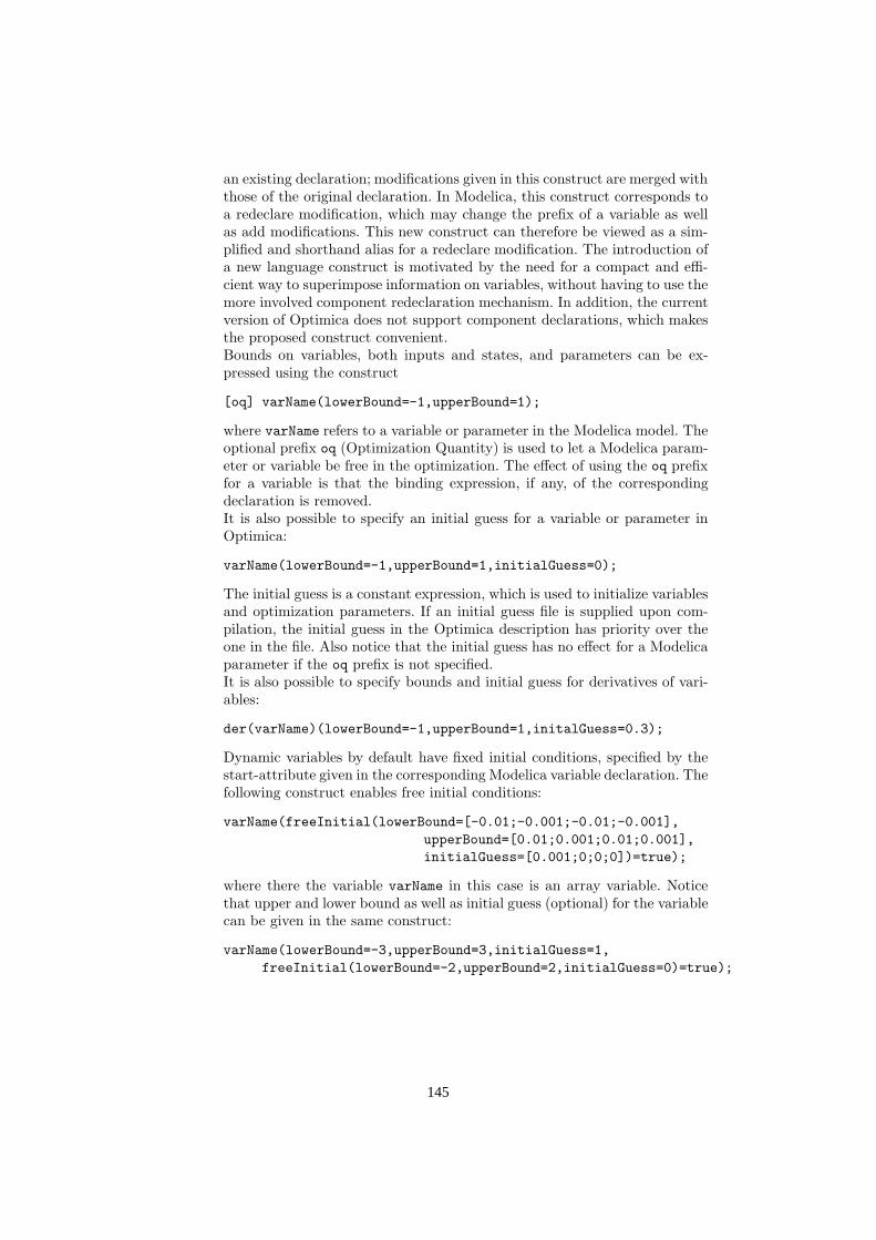
an existing declaration; modifications given in this construct are merged withthose of the original declaration. In Modelica, this construct corresponds toa redeclare modification, which may change the prefix of a variable as wellas add modifications. This new construct can therefore be viewed as a sim-plified and shorthand alias for a redeclare modification. The introduction ofa new language construct is motivated by the need for a compact and effi-cient way to superimpose information on variables, without having to use themore involved component redeclaration mechanism. In addition, the currentversion of Optimica does not support component declarations, which makesthe proposed construct convenient.Bounds on variables, both inputs and states, and parameters can be ex-pressed using the construct

[oq] varName(lowerBound=-1,upperBound=1);

where varName refers to a variable or parameter in the Modelica model. Theoptional prefix oq (Optimization Quantity) is used to let a Modelica param-eter or variable be free in the optimization. The effect of using the oq prefixfor a variable is that the binding expression, if any, of the correspondingdeclaration is removed.It is also possible to specify an initial guess for a variable or parameter inOptimica:

varName(lowerBound=-1,upperBound=1,initialGuess=0);

The initial guess is a constant expression, which is used to initialize variablesand optimization parameters. If an initial guess file is supplied upon com-pilation, the initial guess in the Optimica description has priority over theone in the file. Also notice that the initial guess has no effect for a Modelicaparameter if the oq prefix is not specified.It is also possible to specify bounds and initial guess for derivatives of vari-ables:

der(varName)(lowerBound=-1,upperBound=1,initalGuess=0.3);

Dynamic variables by default have fixed initial conditions, specified by thestart-attribute given in the corresponding Modelica variable declaration. Thefollowing construct enables free initial conditions:

varName(freeInitial(lowerBound=[-0.01;-0.001;-0.01;-0.001],

upperBound=[0.01;0.001;0.01;0.001],

initialGuess=[0.001;0;0;0])=true);

where there the variable varName in this case is an array variable. Noticethat upper and lower bound as well as initial guess (optional) for the variablecan be given in the same construct:

varName(lowerBound=-3,upperBound=3,initialGuess=1,

freeInitial(lowerBound=-2,upperBound=2,initialGuess=0)=true);

145

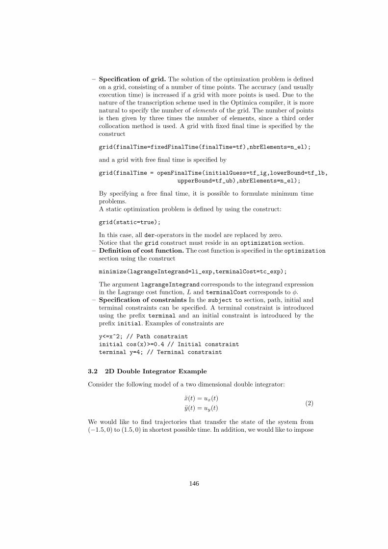
– Specification of grid. The solution of the optimization problem is definedon a grid, consisting of a number of time points. The accuracy (and usuallyexecution time) is increased if a grid with more points is used. Due to thenature of the transcription scheme used in the Optimica compiler, it is morenatural to specify the number of elements of the grid. The number of pointsis then given by three times the number of elements, since a third ordercollocation method is used. A grid with fixed final time is specified by theconstruct

grid(finalTime=fixedFinalTime(finalTime=tf),nbrElements=n_el);

and a grid with free final time is specified by

grid(finalTime = openFinalTime(initialGuess=tf_ig,lowerBound=tf_lb,

upperBound=tf_ub),nbrElements=n_el);

By specifying a free final time, it is possible to formulate minimum timeproblems.A static optimization problem is defined by using the construct:

grid(static=true);

In this case, all der-operators in the model are replaced by zero.Notice that the grid construct must reside in an optimization section.

– Definition of cost function. The cost function is specified in the optimizationsection using the construct

minimize(lagrangeIntegrand=li_exp,terminalCost=tc_exp);

The argument lagrangeIntegrand corresponds to the integrand expressionin the Lagrange cost function, L and terminalCost corresponds to φ.

– Specification of constraints In the subject to section, path, initial andterminal constraints can be specified. A terminal constraint is introducedusing the prefix terminal and an initial constraint is introduced by theprefix initial. Examples of constraints are

y<=x^2; // Path constraint

initial cos(x)>=0.4 // Initial constraint

terminal y=4; // Terminal constraint

3.2 2D Double Integrator Example

Consider the following model of a two dimensional double integrator:

x(t) = ux(t)

y(t) = uy(t)(2)

We would like to find trajectories that transfer the state of the system from(−1.5, 0) to (1.5, 0) in shortest possible time. In addition, we would like to impose

146

−1.5 −1 −0.5 0 0.5 1 1.5−0.2

−0.1

0

0.1

0.2

0.3

0.4

0.5

0.6

0.7

0.8

x

y

States

Constraint

0 0.5 1 1.5 2 2.5 3 3.5 4 4.5−1

−0.8

−0.6

−0.4

−0.2

0

0.2

0.4

0.6

0.8

1

Time [s]

[N]

ux

uy

Fig. 1. Resulting optimization profiles for the minimum time case.

the path constraint y ≥ cosx−0.2 and u2

x+u2

y≤ 1. The latter constraint ensures

that the resulting force has a magnitude equal to or less than 1. This gives usthe following optimal control formulation

minu

∫tf

0

1dt

subject to

x(t) = ux(t)

y(t) = uy(t)

x(0) = −1.5, x(tf ) = 1.5, y(0) = 0, y(tf ) = 0

x(0) = 0, x(tf ) = 0, y(0) = 0, y(tf ) = 0

y(t) ≥ cosx(t) − 0.2

1 ≥ ux(t)2 + uy(t)2

(3)

The dynamics of the double integrator system is given by the following Mod-elica model:

model DoubleIntegrator2d

input Real ux;

input Real uy;

Real x(start=-1.5), vx(start=0);

Real y(start=0), vy(start=0);

equation

der(x)=vx; der(vx)=ux;

der(y)=vy; der(vy)=uy;

end DoubleIntegrator2d;

and the Optimica description of the optimization problem is given by:

147

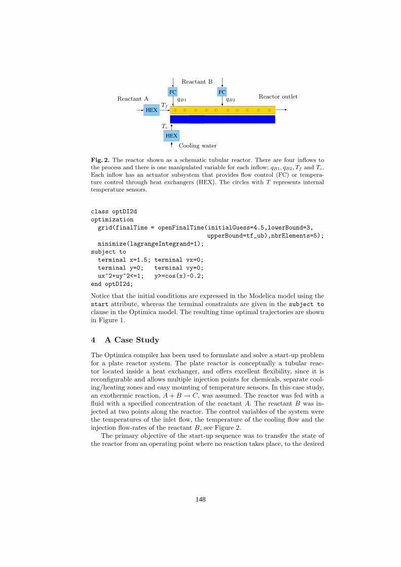
T T T T T T T T T T

FC FC

HEX

HEX

Reactor outletReactant A

Reactant B

Cooling water

qB1 qB2

Tc

Tf

Fig. 2. The reactor shown as a schematic tubular reactor. There are four inflows tothe process and there is one manipulated variable for each inflow; qB1, qB2, Tf and Tc.Each inflow has an actuator subsystem that provides flow control (FC) or tempera-ture control through heat exchangers (HEX). The circles with T represents internaltemperature sensors.

class optDI2d

optimization

grid(finalTime = openFinalTime(initialGuess=4.5,lowerBound=3,

upperBound=tf_ub),nbrElements=5);

minimize(lagrangeIntegrand=1);

subject to

terminal x=1.5; terminal vx=0;

terminal y=0; terminal vy=0;

ux^2+uy^2<=1; y>=cos(x)-0.2;

end optDI2d;

Notice that the initial conditions are expressed in the Modelica model using thestart attribute, whereas the terminal constraints are given in the subject to

clause in the Optimica model. The resulting time optimal trajectories are shownin Figure 1.

4 A Case Study

The Optimica compiler has been used to formulate and solve a start-up problemfor a plate reactor system. The plate reactor is conceptually a tubular reac-tor located inside a heat exchanger, and offers excellent flexibility, since it isreconfigurable and allows multiple injection points for chemicals, separate cool-ing/heating zones and easy mounting of temperature sensors. In this case study,an exothermic reaction, A + B → C, was assumed. The reactor was fed with afluid with a specified concentration of the reactant A. The reactant B was in-jected at two points along the reactor. The control variables of the system werethe temperatures of the inlet flow, the temperature of the cooling flow and theinjection flow-rates of the reactant B, see Figure 2.

The primary objective of the start-up sequence was to transfer the state ofthe reactor from an operating point where no reaction takes place, to the desired

148

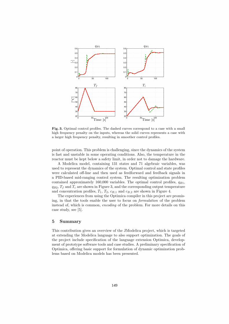
0 50 1000

0.1

0.2

0.3

0.4

0.5

0.6

0 50 1000

0.1

0.2

0.3

0.4

0.5

0.6

0 50 10020

30

40

50

60

70

80

0 50 10020

30

40

50

60

70

80

qB1 qB1

Tf Tc

[C

]

Time [s]Time [s]

[-]

Fig. 3. Optimal control profiles. The dashed curves correspond to a case with a smallhigh frequency penalty on the inputs, whereas the solid curves represents a case witha larger high frequency penalty, resulting in smoother control profiles.

point of operation. This problem is challenging, since the dynamics of the systemis fast and unstable in some operating conditions. Also, the temperature in thereactor must be kept below a safety limit, in order not to damage the hardware.

A Modelica model, containing 131 states and 71 algebraic variables, wasused to represent the dynamics of the system. Optimal control and state profileswere calculated off-line and then used as feedforward and feedback signals ina PID-based mid-ranging control system. The resulting optimization problemcontained approximately 160,000 variables. The optimal control profiles, qB1,qB2, Tf and Tc are shown in Figure 3, and the corresponding output temperatureand concentration profiles, T1, T2, cB,1 and cB,2 are shown in Figure 4.

The experiences from using the Optimica compiler in this project are promis-ing, in that the tools enable the user to focus on formulation of the probleminstead of, which is common, encoding of the problem. For more details on thiscase study, see [5].

5 Summary

This contribution gives an overview of the JModelica project, which is targetedat extending the Modelica language to also support optimization. The goals ofthe project include specification of the language extension Optimica, develop-ment of prototype software tools and case studies. A preliminary specification ofOptimica, offering basic support for formulation of dynamic optimization prob-lems based on Modelica models has been presented.

149

0 50 10020

40

60

80

100

120

140

160

0 50 10020

40

60

80

100

120

140

160

0 50 1000

100

200

300

400

0 50 1000

100

200

300

400

T1 T2

cB,1 cB,2

[C

]

Time [s]Time [s][m

ol/

m3]

[mol/

m3]

Fig. 4. Optimal profiles profiles for reactor temperature and concentration of sub-stance B. The left plots correspond to the first injection point, whereas the right plotscorrespond to the second injection point.

References

1. Johan Akesson, Torbjorn Ekman, and Gorel Hedin. Development of a Modelicacompiler using JastAdd. In Seventh Workshop on Language Descriptions, Toolsand Applications, Braga, Portugal, March 2007.

2. L.T. Biegler, A.M. Cervantes, and A Wchter. Advances in simultaneous strategiesfor dynamic optimization. Chemical Engineering Science, 57:575–593, 2002.

3. T. Ekman and G Hedin. The jastadd extensible java compiler. In Proceedingsof the 22nd Annual ACM SIGPLAN Conference on Object-Oriented Programming,Systems, Languages, and Applications, OOPSLA 2007, Montreal, Canada, October2007. To appear.

4. R. Fourer, D. Gay, and B. Kernighan. AMPL – A Modeling Language for Mathe-matical Programming. Brooks/Cole — Thomson Learning, 2003.

5. Staffan Haugwitz, Johan Akesson, and Per Hagander. Dynamic optimization of aplate reactor start-up supported by Modelica-based code generation software. InProceedings of 8th International Symposium on Dynamics and Control of ProcessSystems, Cancun, Mexico, June 2007.

6. G. Hedin. Reference Attributed Grammars. In Informatica (Slovenia), 24(3), pages301–317, 2000.

7. G. Hedin and E. Magnusson. JastAdd: an aspect-oriented compiler constructionsystem. Science of Computer Programming, 47(1):37–58, 2003.

8. The Modelica Association, 2006. http://www.modelica.org.9. Andreas Wachter and Lorenz T. Biegler. On the implementation of an interior-point

filter line-search algorithm for large-scale nonlinear programming. MathematicalProgramming, 106(1):25–58, 2006.

150

Robust Initialization of Differential Algebraic Equations

Bernhard Bachmann, Peter Aronsson*, Peter Fritzson+

Dept. Mathematics and Engineering, University of Applied Sciences, D-33609 Bielefeld, Germany

bernhard.bachmann@fh-bielefeld.de

* MathCore Engineering AB, Teknikringen 1F, SE-583 30 Linköping, Sweden peter.aronsson@mathcore.com

+ PELAB Programming Environments Lab, Department of Computer Science Linköping University, SE-581 83 Linköping, Sweden

petfr@ida.liu.se

(Previously published in Modelica'2006, Vienna, Sept 4-5, 2006. www.modelica.org)

Abstract. This paper describes a new solution method applied to the problem initializing DAEs using the Modelica lan-guage. Modelica is primarily an ob-ject-oriented equa-tion-based modeling language that allows specification of mathematical models of complex natural or man-made systems. Major features of Modelica are the mul-tidomain modeling capability and the reusability of model components corresponding to physical objects, which allow to build and simulate highly complex sys-tems. However, initializing such models has been quite cumbersome, since initial equations have to be pro-vided at the system level, where the user needs to know details on the underlying transformation and index-reduction algorithms, that in general are applied to simulate a Mode-lica model. .

1 Introduction

So far, using model initialization in Modelica has only been possible for higher-index problems if the user formulates the initial equations globally. This was also the case, e.g. when using the OpenModelica OpenModelica compiler which is an open source implementation developed at PELAB, Linköping University. In order to do such a global formulation successfully, the user needs to know about index reduction, at least the number of freedom left after applying the dummy derivative method is necessary. Therefore, only advanced users have been able to use this feature in the Modelica lan-guage, when higher index problems occur (which is very common). In order to pro-vide a more complete simulation environment, we have started to add robust initiali-zation techniques to the OpenModelica compiler.

151

2 Flattening of a Modelica Model to a Hybrid DAE

A Modelica model is typically translated to a basic mathematical representation in terms of a flat system of differential and algebraic equations (DAEs) before being able to simulate the model. This translation process elaborates on the internal model representation by performing analysis and type checking, inheritance and expansion of base classes, modifications and redeclarations, conversion of connect-equations to basic equations, etc. The result of this analysis and translation process is a flat set of equations, including conditional equations, as well as constants, variables, and func-tion definitions. By the term flat is meant that the object-oriented structure has been broken down to a flat representation where no trace of the object hierarchy remains apart from dot notation (e.g. Class.Subclass.variable) within names.

3 Mathematical Formulation of Hybrid DAEs

3.1 Summary of notation

Below we summarize the notation used in the equations that follow, with time de-pendencies stated explicitly for all time-dependent variables by the arguments t or te:

• ,...,, 21 ppp = a vector containing the Modelica variables declared as parame-ter or constant i.e., variables without any time dependency.

• ,t the Modelica variable time, the independent variable of type Real implicitly occurring in all Modelica models.

• )(tx , the vector of state variables of the model, i.e., variables of type Real that also appear differentiated, meaning that der() is applied to them somewhere in the model.

• )(tx , the differentiated vector of state variables of the model. • )(tu , a vector of input variables, i.e., not dependent on other variables, of type Real. These also belong to the set of algebraic variables since they do not appear differentiated.

• )(ty , a vector of Modelica variables of type Real which do not fall into any other category. Output variables are included among these, which together with )(tu are algebraic variables since they do not appear differentiated.

• )( etq , a vector of discrete-time Modelica variables of type discrete Real, Boolean, Integer or String. These variables change their value only at event instants, i.e., at points te in time.

• )( epre tq , the values of q immediately before the current event occurred, i.e., at time te.

• )( etc , a vector containing all Boolean condition expressions evaluated at the most recent event at time te. This includes conditions from all if-equations/statements and if-expressions from the original model as well as those generated during the conversion of when-equations and when-statements.

152

• ))),(),(,,,,,,1(())(( ptqtqtyuxxcatreltvrel epree= , a Boolean vector val-ued function containing the relevant elementary relational expressions from the model, excluding relations enclosed by noEvent(). The argument v(t) = v1,v2,... is a vector containing all elements in the vectors

ptqtqtyuxx epree ),(),(,,,,, . This can be expressed using the Modelica con-catenation function cat applied to these vectors; rel(v(t)) = v1 > v2, v3 >= 0, v4<5, v6<=v7, v12=133 is one possible example.

• (...)f , the function that defines the differential equations 0(...) =f in (1a) of the system of equations.

• (...)g , the function that defines the algebraic equations 0(...) =g in (1b) of the system of equations.

• (...)qf , the function that defines the difference equations for the discrete vari-ables (...): qfq = , i.e., (2) in the system of equations.

• (...)ef , the function that defines the event conditions (...): efc = , i.e., (3) in the system of equations.

• (...)xf , the function that defines the reinitialization values for the continuous vari-ables (...):)( xe ftx = at events.

In the context of hybrid DAE:s the state of a system is not only made up of the values of the set of variables that occur differentiated in the model. The overall state of a system may also include values of discrete variables. In this paper the word state is used in this sense, including the state of the discrete part of the system.

3.2 Continuous-Time Behavior

Now we want to formulate the continuous part of the hybrid DAE system of equations including discrete variables. This is done by adding a vector q(te) of discrete-time variables and the corresponding predecessor variable vector qpre(te) denoted by pre(q) in Modelica. For discrete variables we use te instead of t to indicate that such variables may only change value at event time points denoted te, i.e., the variables q(te) and qpre(te) behave as constants between events.

We also make the constant vector p of parameters and constants explicit in the equations, and make the time t explicit. The vector c(te) of condition expressions, e.g. from the conditions of if constructs and when constructs, evaluated at the most recent event at time te is also included since such conditions are referenced in condi-tional equations. We obtain the following continuous DAE system of equations that describe the system behavior between events:

0))(,),(),(,),(),(),((

0))(,),(),(,),(),(),(),((

=

=

eepree

eepree

tcptqtqttytutxgtcptqtqttytutxtxf

)()(

ba

(1)

153

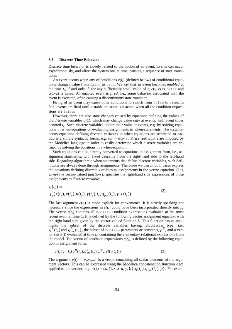
3.3 Discrete-Time Behavior

Discrete time behavior is closely related to the notion of an event. Events can occur asynchronously, and affect the system one at time, causing a sequence of state transi-tions.

An event occurs when any of conditions c(te) (defined below) of conditional equa-tions changes value from false to true. We say that an event becomes enabled at the time te, if and only if, for any sufficiently small value of ε, c(te-ε) is false and c(te+ε) is true. An enabled event is fired, i.e., some behavior associated with the event is executed, often causing a discontinuous state transition.

Firing of an event may cause other conditions to switch from false to true. In fact, events are fired until a stable situation is reached when all the condition expres-sions are false.

However, there are also state changes caused by equations defining the values of the discrete variables q(te), which may change value only at events, with event times denoted te. Such discrete variables obtain their value at events, e.g. by solving equa-tions in when-equations or evaluating assignments in when-statements. The instanta-neous equations defining discrete variables in when-equations are restricted to par-ticularly simple syntactic forms, e.g. var = expr;. These restrictions are imposed by the Modelica language in order to easily determine which discrete variables are de-fined by solving the equations in a when-equation.

Such equations can be directly converted to equations in assignment form, i.e., as-signment statements, with fixed causality from the right-hand side to the left-hand side. Regarding algorithmic when-statements that define discrete variables, such defi-nitions are always done through assignments. Therefore we can in both cases express the equations defining discrete variables as assignments in the vector equation (1a), where the vector-valued function fq specifies the right-hand side expressions of those assignments to discrete variables.

( ) :( ( ), ( ), ( ), ( ), , ( ), , ( ))e

q e e e e e pre e e

q tf x t x t u t y t t q t p c t

= (2)

The last argument c(te) is made explicit for convenience. It is strictly speaking not necessary since the expressions in c(te) could have been incorporated directly into fq. The vector c(te) contains all Boolean condition expressions evaluated at the most recent event at time te. It is defined by the following vector assignment equation with the right-hand side given by the vector-valued function fe. This function has as argu-ments the subset of the discrete variables having Boolean type, i.e.,

)( eB tq and )( e

Bpre tq , the subset of Boolean parameters or constants, Bp , and a vec-

tor rel(v(t)) evaluated at time te, containing the elementary relational expressions from the model. The vector of condition expressions c(te) is defined by the following equa-tion in assignment form:

)))((,),(),((:)( eB

eBpree

Bee tvrelptqtqftc = (3)

The argument v(t) = v1,v2,... is a vector containing all scalar elements of the argu-ment vectors. This can be expressed using the Modelica concatenation function cat applied to the vectors, e.g. )),(),(,,,,,,1()( ptqtqtyuxxcattv epree= . For exam-

154

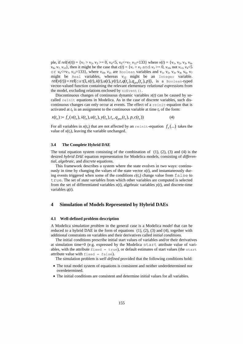
ple, if rel(v(t)) = v1 > v2, v3 >= 0, v4<5, v6<=v7, v12=133 where v(t) = v1, v2, v3, v4, v6, v7, v12, then it might be the case that c(t) = v1 > v2 and v3 >= 0, v10, not v11, v4<5 or v6<=v7, v12=133, where v10, v11 are Boolean variables and v1, v2, v3, v4, v6, v7 might be Real variables, whereas v12 might be an Integer variable.

))),(),(,),(),(),(),(,1(())(( ptqtqttytutxtxreltvrel epreecat= , is a Boolean-typed vector-valued function containing the relevant elementary relational expressions from the model, excluding relations enclosed by noEvent().

Discontinuous changes of continuous dynamic variables x(t) can be caused by so-called reinit equations in Modelica. As in the case of discrete variables, such dis-continuous changes can only occur at events. The effect of a reinit-equation that is activated at te is an assignment to the continuous variable at time te of the form:

))(,),(,),(),(),(),((:)( eepreeeeeexe tcptqttytutxtxftx = (4)

For all variables in x(te) that are not affected by an reinit-equation (...)xf takes the value of x(te), leaving the variable unchanged..

3.4 The Complete Hybrid DAE

The total equation system consisting of the combination of (1), (2), (3) and (4) is the desired hybrid DAE equation representation for Modelica models, consisting of differen-tial, algebraic, and discrete equations.

This framework describes a system where the state evolves in two ways: continu-ously in time by changing the values of the state vector x(t), and instantaneously dur-ing events triggered when some of the conditions c(te) change value from false to true. The set of state variables from which other variables are computed is selected from the set of differentiated variables x(t), algebraic variables y(t), and discrete-time variables q(t).

4 Simulation of Models Represented by Hybrid DAEs

4.1 Well-defined problem description

A Modelica simulation problem in the general case is a Modelica model that can be reduced to a hybrid DAE in the form of equations (1), (2), (3) and (4), together with additional constraints on variables and their derivatives called initial conditions.

The initial conditions prescribe initial start values of variables and/or their derivatives at simulation time=0 (e.g. expressed by the Modelica start attribute value of vari-ables, with the attribute fixed = true), or default estimates of start values (the start attribute value with fixed = false).

The simulation problem is well defined provided that the following conditions hold:

• The total model system of equations is consistent and neither underdetermined nor overdetermined.

• The initial conditions are consistent and determine initial values for all variables.

155

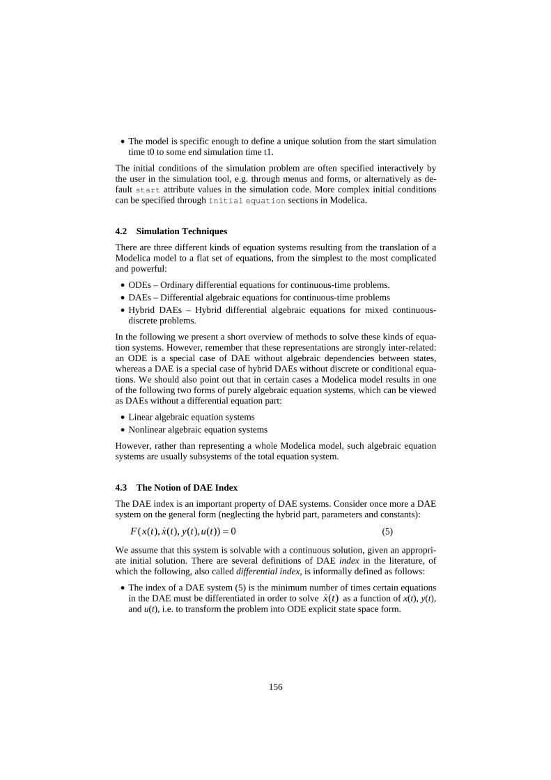
• The model is specific enough to define a unique solution from the start simulation time t0 to some end simulation time t1.

The initial conditions of the simulation problem are often specified interactively by the user in the simulation tool, e.g. through menus and forms, or alternatively as de-fault start attribute values in the simulation code. More complex initial conditions can be specified through initial equation sections in Modelica.

4.2 Simulation Techniques

There are three different kinds of equation systems resulting from the translation of a Modelica model to a flat set of equations, from the simplest to the most complicated and powerful:

• ODEs – Ordinary differential equations for continuous-time problems. • DAEs – Differential algebraic equations for continuous-time problems • Hybrid DAEs – Hybrid differential algebraic equations for mixed continuous-

discrete problems.

In the following we present a short overview of methods to solve these kinds of equa-tion systems. However, remember that these representations are strongly inter-related: an ODE is a special case of DAE without algebraic dependencies between states, whereas a DAE is a special case of hybrid DAEs without discrete or conditional equa-tions. We should also point out that in certain cases a Modelica model results in one of the following two forms of purely algebraic equation systems, which can be viewed as DAEs without a differential equation part:

• Linear algebraic equation systems • Nonlinear algebraic equation systems

However, rather than representing a whole Modelica model, such algebraic equation systems are usually subsystems of the total equation system.

4.3 The Notion of DAE Index

The DAE index is an important property of DAE systems. Consider once more a DAE system on the general form (neglecting the hybrid part, parameters and constants):

0))(),(),(),(( =tutytxtxF (5)

We assume that this system is solvable with a continuous solution, given an appropri-ate initial solution. There are several definitions of DAE index in the literature, of which the following, also called differential index, is informally defined as follows:

• The index of a DAE system (5) is the minimum number of times certain equations in the DAE must be differentiated in order to solve )(tx as a function of x(t), y(t), and u(t), i.e. to transform the problem into ODE explicit state space form.

156

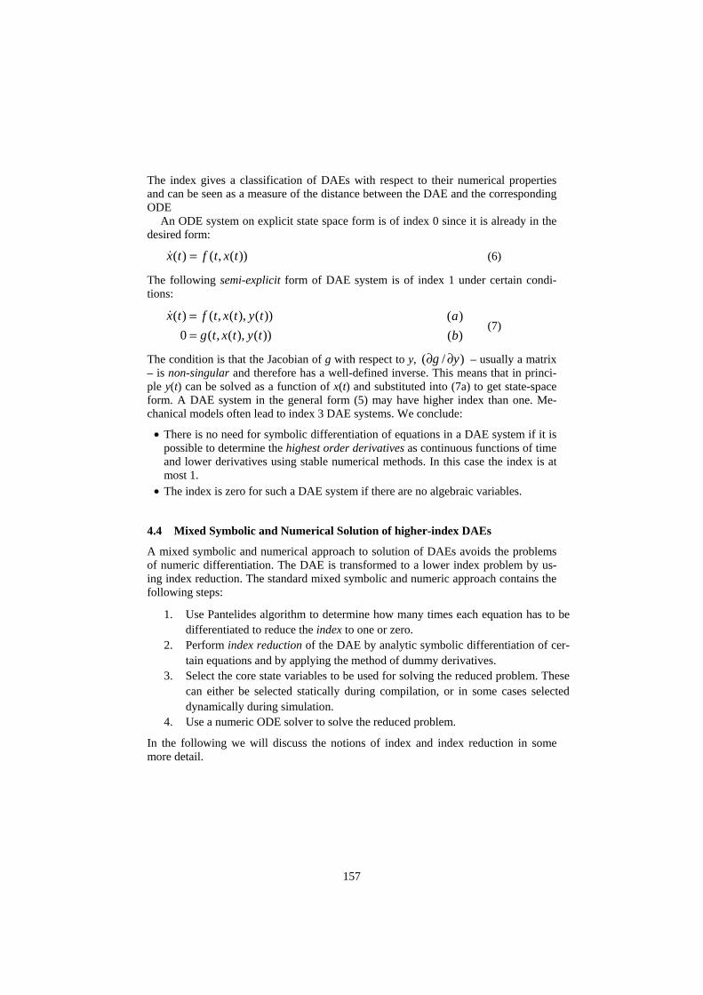
The index gives a classification of DAEs with respect to their numerical properties and can be seen as a measure of the distance between the DAE and the corresponding ODE

An ODE system on explicit state space form is of index 0 since it is already in the desired form:

))(,()( txtftx = (6)

The following semi-explicit form of DAE system is of index 1 under certain condi-tions:

))(),(,(0))(),(,()(

tytxtgtytxtftx

==

)()(

ba

(7)

The condition is that the Jacobian of g with respect to y, )/( yg ∂∂ – usually a matrix – is non-singular and therefore has a well-defined inverse. This means that in princi-ple y(t) can be solved as a function of x(t) and substituted into (7a) to get state-space form. A DAE system in the general form (5) may have higher index than one. Me-chanical models often lead to index 3 DAE systems. We conclude:

• There is no need for symbolic differentiation of equations in a DAE system if it is possible to determine the highest order derivatives as continuous functions of time and lower derivatives using stable numerical methods. In this case the index is at most 1.

• The index is zero for such a DAE system if there are no algebraic variables.

4.4 Mixed Symbolic and Numerical Solution of higher-index DAEs

A mixed symbolic and numerical approach to solution of DAEs avoids the problems of numeric differentiation. The DAE is transformed to a lower index problem by us-ing index reduction. The standard mixed symbolic and numeric approach contains the following steps:

1. Use Pantelides algorithm to determine how many times each equation has to be differentiated to reduce the index to one or zero.

2. Perform index reduction of the DAE by analytic symbolic differentiation of cer-tain equations and by applying the method of dummy derivatives.

3. Select the core state variables to be used for solving the reduced problem. These can either be selected statically during compilation, or in some cases selected dynamically during simulation.

4. Use a numeric ODE solver to solve the reduced problem.

In the following we will discuss the notions of index and index reduction in some more detail.

157

4.5 Higher Index Problems are Natural in Component-Based Models

The index of a DAE system is not a property of the modeled system but the property of a particular model representation, and therefore a function of the modeling meth-odology. A natural object-oriented component-based methodology with reuse and connections between physical objects leads to high index in the general case. The rea-son is the constraint equations resulting from setting variables equal across connec-tions between separate objects.

Since the index is not a property of the modeled system it is possible to reduce the index by symbolic manipulations. High index indicates that the model has algebraic relations between differentiated state variables implied by algebraic relations between those state variables. By using knowledge about the particular modeling domain it is often possible to manually eliminate a number of differentiated variables, and thus reduce the index. However, this violates the object-oriented component-based model-ing methodology for physical modeling that is intended to be supported by the Mode-lica language.

We conclude that high index models are natural, and that automatic index reduc-tion is necessary to support a general object-oriented component-based modeling methodology with a high degree of reuse.

5 Finding Consistent Initial Values at Start or Restart

As we have stated briefly above, at the start of the simulation, or at restart after han-dling an event, it is required to find a consistent set of initial values or restart values of the variables of the hybrid DAE equation system before starting continuous DAE so-lution process.

At the start of the simulation these conditions are given by the initial conditions of the problems (including start attribute equations, equations in initial equation sections, etc., together with the system of equations defined by (1), (2), and (3). The user specifies the initial time of the simulation, t0, and initial values or guesses of ini-tial values of some of the continuous variables, derivatives, and discrete-time vari-ables so that the algebraic part of the equation system can be solved at the initial time t=t0 for all the remaining unknown initial values. In some application examples it is even necessary to calculate initial values of parameters (fixed = false), that af-terwards be kept constant during simulation.

At restart after an event, the conditions are given by the new values of variables that have changed at the event, together with the current values of the remaining vari-ables, and the system of equations (5), (6), and (7). The goal is the same as in the ini-tial case, to solve for the new values of the remaining variables. In the initial case, however, the causality can be different since initial equations are included to calculate start values for the state variables, whereas at restart the state variables are always known.

158

6 Robust Initialization of Higher-Index DAEs

Initializing DAEs using the Modelica language has been quite cumbersome in the past, since initial equations have to be provided on the system level, where the user needs to know details on the underlying transformation and index-reduction algo-rithms, that are in general applied to simulate a Modelica model. Especially, when higher-index DAEs are involved the number of locally defined state variables no longer coincide with the number of state variables of the overall system. Although, one can influence the index-reduction algorithm by setting some attribute values (stateSelect=always,prefer,…), cases can be constructed which don’t allow the straight forward prediction of the number of state variables left after transforma-tion.

In order to make the initialization procedure more convenient a new concept is necessary, which allows to define the initial equations locally in each relevant compo-nent where the corresponding states appear, even if these states are eliminated during index-reduction. Naturally, this leads to an overdetermined system of equations, which has to be solved during the initialization process. In this context, we call a higher-index problem “well-posed” if enough equations of the system are redundant so that initial values can be determined which fulfill the whole set of initial equations. The main idea of the new approach is to reformulate the problem of finding roots of the set of non-linear equations to an equivalent optimization problem.

Considering the general mathematical description of the initialization problem:

1 1

1

( , ..., ) 0

( ,..., ) 0

n

m n

f z z

f z z

=

=

(8)

Cases where m n≥ means that more equations (m) than variables (n) are given. Every solution to (8) minimizes the problem:

( ) 21 1

1,..., ( ,..., ) min

m

n i ni

F z z f z z=

= →∑ (9)

On the other hand, every global minimum of (9) is a solution to (8). In order to solve (9) a number of different algorithms have been developed during the past. The algo-rithm can be categorized depending on the order of derivatives needed during the so-lution process. In the OpenModelica environment the Simplex-method of Nelder and Mead as well as the Brent’s method are currently implemented, only working with the minimization function F. The OpenModelica prototype already shows reliable results for the evaluated examples.

Further improvements can be achieved as soon as the Jacobian of F with regards to the unknown is available. In that case, more advanced algorithms like the method of Fletcher-Reeves, Quasi-Newton, and/or Levenberg-Marquardt methods can be applied which would provide a speed-up in convergence. We regard this as a quality of im-plementation, since the described approach is working in principle already.

159

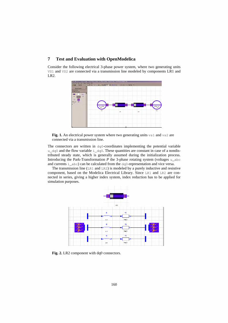
7 Test and Evaluation with OpenModelica

Consider the following electrical 3-phase power system, where two generating units VS1 and VS2 are connected via a transmission line modeled by components LR1 and LR2.

Fig. 1. An electrical power system where two generating units vs1 and vs2 are connected via a transmission line.

The connectors are written in dq0-coordinates implementing the potential variable u_dq0 and the flow variable i_dq0. These quantities are constant in case of a nondis-tributed steady state, which is generally assumed during the initialization process. Introducing the Park-Transformation P the 3-phase rotating system (voltages u_abc and currents i_abc) can be calculated from the dq0-representation and vice versa.

The transmission line (LR1 and LR2) is modeled by a purely inductive and resistive component, based on the Modelica Electrical Library. Since LR1 and LR2 are con-nected in series, giving a higher index system, index reduction has to be applied for simulation purposes.

Fig. 2. LR2 component with dq0 connectors.

160

The voltage source is described similarly using the Modelica Standard Library com-bined with the dq0-connectors.

Fig. 3. Voltage source.

In order to initialize the model correctly to steady state the following initial equations have been added to the local components LR1 and LR2. model LR ... equation ... initial equation der(dq0_1.i_dq0)=0,0,0; end LR;

Due to the higher-index of the overall system, index-reduction is applied. The system finally is determined by 3 state variables LR1.I1.i, LR1.I2.i, LR1.I3.i. The cor-responding initial equation system has 3 equations more than number of unknowns, but these equations are redundant and could be eliminated. Due to the involvement of the Park-transformation, redundancy is not easy to detect. However, applying the con-cept described above correct initialization of the system is performed.

8 Conclusions and Future work

In this paper we have presented an overview of our implementation of initializing Modelica models in the OpenModelica compiler. A new concept has been developed to describe the initial equations locally in the relevant component where the corre-sponding states appear, that also works for arbitrary well-posed higher-index prob-lems. Due to the necessary index reduction some of the states get changed to dummy states that means that they will be algebraic during the simulation of the model. The

161

corresponding initial equations are therefore redundant, but can be handled correctly by the new initialization process, if they are consistent. If not, an error/warning is is-sued to the user.

The described method has been implemented in the OpenModelica compiler. In the future we also wish to implement calculation of the Jacobian matrix of the equation system with regards to the state variables. This gives the possibility to implement more advanced and robust numerical algorithms in order to solve the corresponding optimization (minimization) problem during initialization of the DAE.

9 Acknowledgements

This work was supported by the University of Applied Sciences in Bielefeld, by MathCore Engineering AB, by the Swedish Research Council (VR), and by SSF in the VISIMOD project.

References [1] Peter Fritzson, et al. The Open Source Modelica Project. In Proceedings of The 2nd In-

ternational Modelica Conference, 18-19 March, 2002. Munich, Germany See also: http://www.ida.liu.se/projects/OpenModelica.

[2] Peter Fritzson. Principles of Object-Oriented Modeling and Simulation with Modelica 2.1, 940 pp., ISBN 0-471-471631, Wiley-IEEE Press, 2004.

[3] The Modelica Association. The Modelica Language Specification Version 2.2, March 2005. http://www.modelica.org.

[4] The OpenModelica Users Guide, version 0.6, June 2005. www.ida.liu.se/projects/OpenModelica

[5] The OpenModelica System Documentation, version 0.6, June 2006. www.ida.liu.se/projects/OpenModelica

[6] K. E. Brenan, S. L. Campbell, and L. R. Petzold, Numerical Solution of Initial-Value Problems in Differential-Algebraic Equations, Elsevier, New York, 1989.

[7] B. Bachmann et. al. (Modelica Association): Modelica - A Unified Object-Oriented Lan-guage for Physical Systems Modeling - Language Specification. 2002.

[8] P. Fritzson, P. Aronsson, P. Bunus, V. Engelson, L. Saldamli, H. Johansson, A. Kar-ström: The Open Source Modelica Project. In: 2nd Modelica Conference 2002, Oberpfaf-fenhofen, 2002

[9] S.-E. Mattson, H. Olson, H. Elmqvist: Dynamic Selection of States in Dymola. In: 1st Modelica Workshop 2000, Lund, Sweden, 2000

[10] M. Otter: Objektorientierte Modellierung Physikalischer Systeme (Teil 4) – Transforma-tionsalgorithmen. In: at Automatisierungstechnik, Oldenbourg Verlag München, 1999

[11] M. Otter, B. Bachmann: Objektorientierte Modellierung Physikalischer Systeme (Teil 5,6) – Singuläre Systeme. In: at Automatisierungstechnik, Oldenbourg Verlag München, 1999

[12] R. Fletcher: Practical Methods of Optimization John Wiley & Sons, 1995 [13] J. Stoer, R. Burlisch: Einführung in die numerische Mathematik. Springer Verlag, 1994 [14] S.E. Mattsson, G. Söderlind: Index reduction in differential-algebraic equations using

dummy derivatives. SIAM Journal of Scientific and Statistical Computing, Vol. 14, 1993.

162

[15] K.E. Brenan., S.L. Campbell, L.R. Petzold: Numerical Solution of Initial Value Problems in Differential Algebraic Equations. North-Holland, Amsterdam, 1989

[16] C.C. Pantelides: The Consistent Initialization of Differential-Algebraic Systems, SIAM Journal of Scientific and Statistical Computing, 1988.

[17] L.R. Petzold: A description of DASSL: A differential / algebraic system solver. Sandia National Laboratories, Albuquerque, 1982

[18] H. Elmqvist: A Structured Model Language for Large Continuous Systems, PhD disserta-tion, Department of Automatic Control, Lund Institute of Technology, Lund, Schweden, 1978

[19] R.E. Tarjan: Depth First Search and Linear Graph Algorithms. SIAM Journal of Comp., Nr. 1, 1972

163