Mixed Domain Modeling in Modelica -...
47
1 FDL‘2002, Marseille, September 24 – 27 Mixed Domain Modeling in Modelica C. Clauss 1 , H. Elmqvist 3 , S. E. Mattsson 3 , M. Otter 2 , P. Schwarz 1 1 Fraunhofer Institute for Integrated Circuits, Design Automation Department, EAS, Dresden, Germany 2 German Aerospace Center (DLR), Oberpfaffenhofen, Germany 3 Dynasim AB, Lund, Sweden
-
Upload
nguyenkien -
Category
Documents
-
view
228 -
download
2
Transcript of Mixed Domain Modeling in Modelica -...
1FDL‘2002, Marseille, September 24 – 27
Mixed Domain Modeling in Modelica
C. Clauss1, H. Elmqvist3, S. E. Mattsson3, M. Otter2, P. Schwarz1
1 Fraunhofer Institute for Integrated Circuits, Design Automation Department, EAS, Dresden, Germany
2 German Aerospace Center (DLR), Oberpfaffenhofen, Germany
3 Dynasim AB, Lund, Sweden

2FDL‘2002, Marseille, September 24 – 27
1. Motivation
2. Modelica Fundamentals
3. Modelica Language Elements
4. Simulation Algorithm – Related to the Dymola Simulator
5. Modelica Libraries
6. Application Examples
7. Comparison: VHDL-AMS and Modelica
8. Conclusions
Contents

3FDL‘2002, Marseille, September 24 – 27
Modelica – yet another modeling language: why?
VHDL-AMS, Verilog-AMS, SystemC-AMS have their roots in digital electronics,with extensions to heterogeneous systems:- analog/digital, mixed-signal- HW/SW, digital signal processing- multi-domain capabilities
(e.g., in VHDL-AMS: THROUGH and ACROSS quantities instead of currents andvoltages, NATURE attribute)
Modelica combines some of their features, together with - object-oriented modeling and object-oriented programming- orientation on advanced simulation algorithms, e.g., to avoid index problems
( but this is not part of language definition )
Other languages:Dymola, gPROMS, NMF, ObjectMath, Omola, Smile, U.L.M, EcoSim, ...have their roots in control systems, robotics, hydraulics, and mechatronics
1. Motivation

4FDL‘2002, Marseille, September 24 – 27
• Goal: Technique for multi-domain modeling of complex systems.
• Development started in 1978 by Hilding Elmqvist at Lund Institute of Technology(Sweden).
Summary of some features
Standardisation with the freely available modeling language
• Developed by the (non-profit) Modelica Association since 1996,
• differential, algebraic and discrete equations,
• declarative (= mathematical equations) and procedural (optional) ,
• many Modelica libraries available (mostly public domain):1D/3D Mechanics, electronics, hydraulics, power systems, heat transfer,thermo-fluid pipe flow, flight dynamics, input/output, ... .
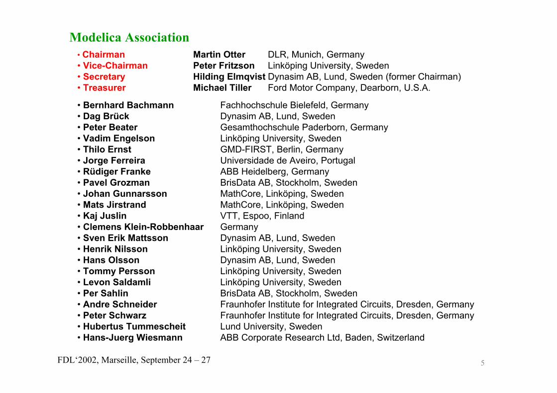
5FDL‘2002, Marseille, September 24 – 27
Modelica Association• Chairman Martin Otter DLR, Munich, Germany• Vice-Chairman Peter Fritzson Linköping University, Sweden • Secretary Hilding Elmqvist Dynasim AB, Lund, Sweden (former Chairman) • Treasurer Michael Tiller Ford Motor Company, Dearborn, U.S.A.
• Bernhard Bachmann Fachhochschule Bielefeld, Germany• Dag Brück Dynasim AB, Lund, Sweden• Peter Beater Gesamthochschule Paderborn, Germany• Vadim Engelson Linköping University, Sweden • Thilo Ernst GMD-FIRST, Berlin, Germany• Jorge Ferreira Universidade de Aveiro, Portugal• Rüdiger Franke ABB Heidelberg, Germany• Pavel Grozman BrisData AB, Stockholm, Sweden• Johan Gunnarsson MathCore, Linköping, Sweden• Mats Jirstrand MathCore, Linköping, Sweden• Kaj Juslin VTT, Espoo, Finland• Clemens Klein-Robbenhaar Germany• Sven Erik Mattsson Dynasim AB, Lund, Sweden• Henrik Nilsson Linköping University, Sweden• Hans Olsson Dynasim AB, Lund, Sweden• Tommy Persson Linköping University, Sweden• Levon Saldamli Linköping University, Sweden • Per Sahlin BrisData AB, Stockholm, Sweden• Andre Schneider Fraunhofer Institute for Integrated Circuits, Dresden, Germany• Peter Schwarz Fraunhofer Institute for Integrated Circuits, Dresden, Germany• Hubertus Tummescheit Lund University, Sweden• Hans-Juerg Wiesmann ABB Corporate Research Ltd, Baden, Switzerland

6FDL‘2002, Marseille, September 24 – 27
Homepage: www.Modelica.org
Tutorial: www.Modelica.org/current/ModelicaTutorial14.pdf
Formal specification: www.Modelica.org/current/ModelicaSpecification14.pdf
Model libraries: www.Modelica.org/library/library.html
Publications: www.Modelica.org/workshop2000/proceedings
www.Modelica.org/workshop2002/proceedings
Tools (simulators): www.Modelica.org/tools.shtml
Dymola (www.Dynasim.se)MathModelica (www.MathCore.se)
7FDL‘2002, Marseille, September 24 – 27
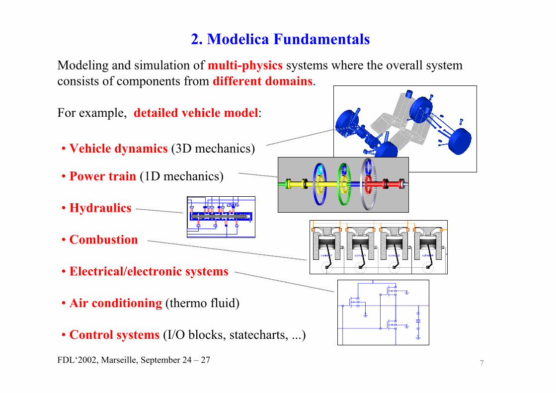
Modeling and simulation of multi-physics systems where the overall system consists of components from different domains.
For example, detailed vehicle model:
• Vehicle dynamics (3D mechanics)
• Power train (1D mechanics)
• Hydraulics
• Combustion
• Electrical/electronic systems
• Air conditioning (thermo fluid)
• Control systems (I/O blocks, statecharts, ...)
2. Modelica Fundamentals

8FDL‘2002, Marseille, September 24 – 27
Composition Diagrams of Modelica (= object diagrams)
component
• Every Icon represents a physical component.e.g. electrical resistance, mechanical gear, pump
connection
• The connection lines represent the actual physical connection.E.g.: electrical line, rigid mechanical connection, heat flow between components.
Interface
• Variables in the interface points define the couplingwith other objects
• A component consists of a connection of components(= hierarchical structure) and/or is described by equations
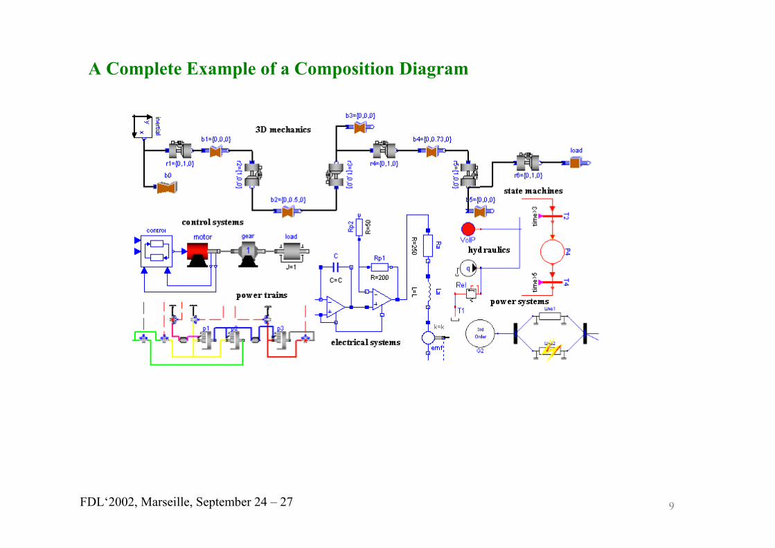
9FDL‘2002, Marseille, September 24 – 27
A Complete Example of a Composition Diagram
10FDL‘2002, Marseille, September 24 – 27
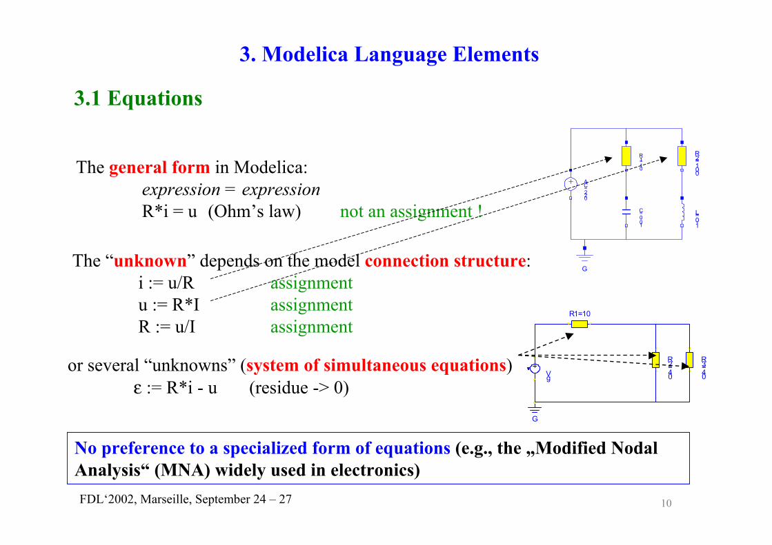
The general form in Modelica:expression = expressionR*i = u (Ohm’s law) not an assignment !
3. Modelica Language Elements
3.1 Equations
R1=10
AC=220
C=0.01
G
R2=100
L=0.1
The “unknown” depends on the model connection structure:i := u/R assignmentu := R*I assignmentR := u/I assignment
Vg
R1=10
R2=40
G
R3=40
or several “unknowns” (system of simultaneous equations)ε := R*i - u (residue -> 0)
No preference to a specialized form of equations (e.g., the „Modified NodalAnalysis“ (MNA) widely used in electronics)
11FDL‘2002, Marseille, September 24 – 27
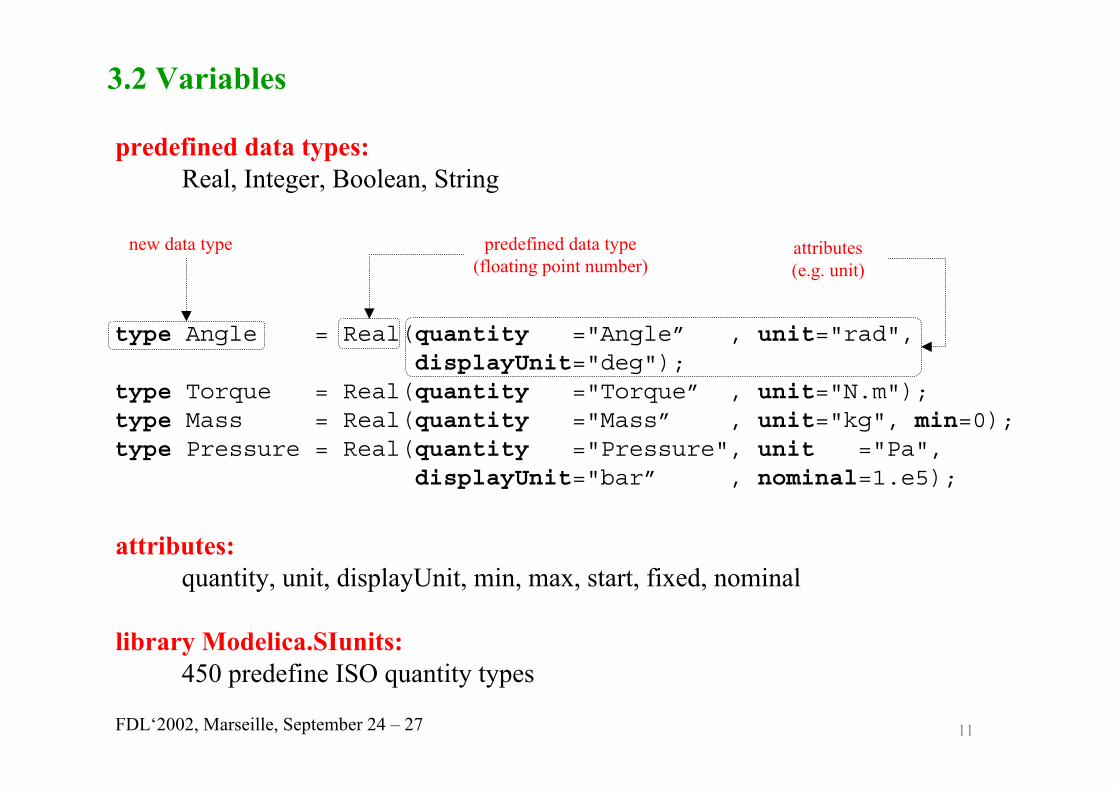
type Angle = Real(quantity ="Angle” , unit="rad",displayUnit="deg");
type Torque = Real(quantity ="Torque” , unit="N.m");type Mass = Real(quantity ="Mass” , unit="kg", min=0);type Pressure = Real(quantity ="Pressure", unit ="Pa",
displayUnit="bar” , nominal=1.e5);
predefined data type(floating point number)
attributes(e.g. unit)
3.2 Variables
attributes:quantity, unit, displayUnit, min, max, start, fixed, nominal
new data type
predefined data types:Real, Integer, Boolean, String
library Modelica.SIunits:450 predefine ISO quantity types
12FDL‘2002, Marseille, September 24 – 27
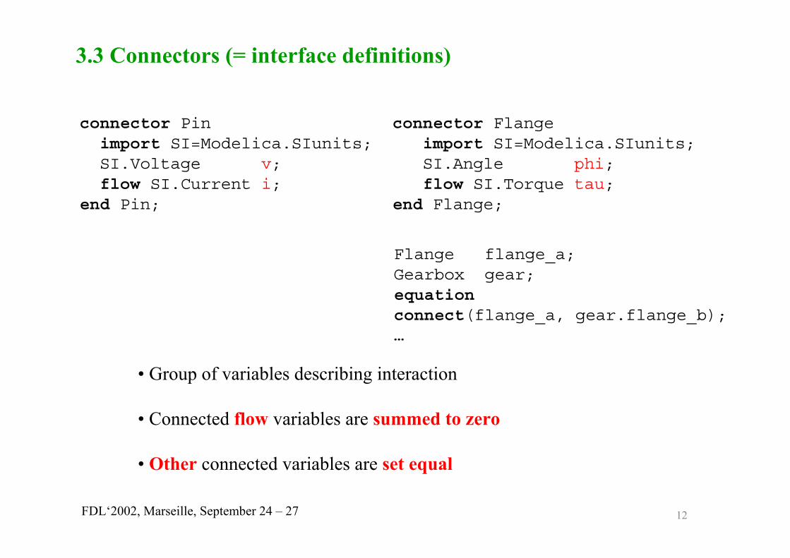
connector Pin connector Flangeimport SI=Modelica.SIunits; import SI=Modelica.SIunits;SI.Voltage v; SI.Angle phi;flow SI.Current i; flow SI.Torque tau;
end Pin; end Flange;
3.3 Connectors (= interface definitions)
Flange flange_a;Gearbox gear;equationconnect(flange_a, gear.flange_b);…
• Group of variables describing interaction
• Connected flow variables are summed to zero
• Other connected variables are set equal

13FDL‘2002, Marseille, September 24 – 27
electrical 1D translational mechanics
321
31
21
0 iiivvvv
++===
321
31
21
0 fffssss
++===
connect(R1.p, R2.p);connect(R1.p, R3.p);
connect(m1.flange_a, m2.flange_a);connect(m1.flange_a, m3.flange_a);
i1
i3
i2
v1v3 v2
R1
R3
R2
f1 f2
f3
s1
s3
s2
m1 m3
m3
Generated statements:
Connectors

14FDL‘2002, Marseille, September 24 – 27
model IdealPlanetaryparameter Real ratio=100/50 ”# ring_teeth/sun_teeth";Flange sun "sun flange";Flange carrier "carrier flange ";Flange ring "ring flange";
equation// kinematic relationshipsun.phi - carrier.phi + ratio*(ring.phi - carrier.phi) = 0;
// torque balance (no inertias)ring.tau = ratio*sun.tau;carrier.tau + sun.tau + ring.tau = 0;
end IdealPlanetary
ideal planetary gear box (no inertias)
3.4 Component models
15FDL‘2002, Marseille, September 24 – 27
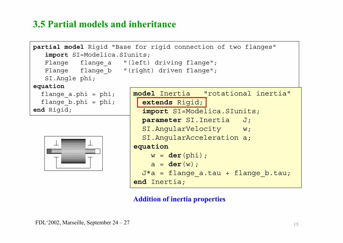
partial model Rigid "Base for rigid connection of two flanges"import SI=Modelica.SIunits;Flange flange_a "(left) driving flange";Flange flange_b "(right) driven flange";SI.Angle phi;
equationflange_a.phi = phi;flange_b.phi = phi;
end Rigid;
3.5 Partial models and inheritance
model Inertia "rotational inertia"extends Rigid;import SI=Modelica.SIunits;parameter SI.Inertia J;SI.AngularVelocity w;SI.AngularAcceleration a;
equationw = der(phi);a = der(w);
J*a = flange_a.tau + flange_b.tau;end Inertia;
Addition of inertia properties

16FDL‘2002, Marseille, September 24 – 27
SingleOutput
Source
SineSource
Function
Sine
f
f
OnePort
VoltageSource
SineVoltage
Inheritance(is-a-relation)
Composition (has-a-relation)
s
s
3.5 Partial models and inheritance (cont‘d)
VoltageSource
Source
time x y o
p
n
vFunction
Example: electrical voltage sources

17FDL‘2002, Marseille, September 24 – 27
3.6 Model composition
model SimpleCarimport Modelica.Mechanics.Translational.Sensors;Car.Driver driver (k=30, T=50);Car.FullGear gearbox(tableFile="ZF4HP22.dat");Car.FullEngine engine (tableFile="engine1.dat");Car.Resistance car(mass=1800, area=2.0, ...);Car.Axle axleSensors.SpeedSensor v;
equationconnect(car.flange_a , v.flange_a);connect(gearbox.flange_a, engine.flange_b);connect(gearbox.flange_b, axle.SteeringWheel);connect(axle.flange_b , car.flange_a);connect(driver.throttle , engine.inPort);connect(v.outPort , driver.speed);connect(driver.throttle , gearbox.inPort);connect(driver.brake , axle.inPort);
end SimpleCar;
annotation(extent=[20, -10; 40, 10]);

18FDL‘2002, Marseille, September 24 – 27
File: ...\Modelica\Electrical\Analog\Basic.mo
within Modelica.Electrical.Analog;package Basic
model Resistor...
end Resistor;
model Capacitor...
end Capacitor;...
end Basic;
\Modelica\Blocks\Electrical
\AnalogBasic.moSemiconductors.moSources.mo
...\Mechanics
Rotational.moTranslational.mo
Constants.moIcons.moMath.moSIunits.mo
...
Modelica libraries are hierarchically structured and are mapped to the same hierarchy of the file system (i.e. file name = model name):
new library
3.7 Component libraries
Example: Modelica.Electrical.Analog.Basic

19FDL‘2002, Marseille, September 24 – 27
• Prozedural sections (algorithm)
• if, for, while
• Functions, including well defined external C function interface
• Multidimensional arrays (similiar to Matlab)
• Multidimensional component arrays (e.g. for PDE discretization)
• Replaceable model components (replaceable/redeclare)
• Discrete equations (when; e.g. sampled data systems)
• Discontinuous equations (time- and state events)
• Variable structure equations (e.g. friction, clutches, ideal diode)
• Very general initialization (if initial() then ... end if)
• Re-initialization at events (impulse(..))
• Graphical annotations and embedding of icons
3.8 Additional language elements of Modelica
20FDL‘2002, Marseille, September 24 – 27
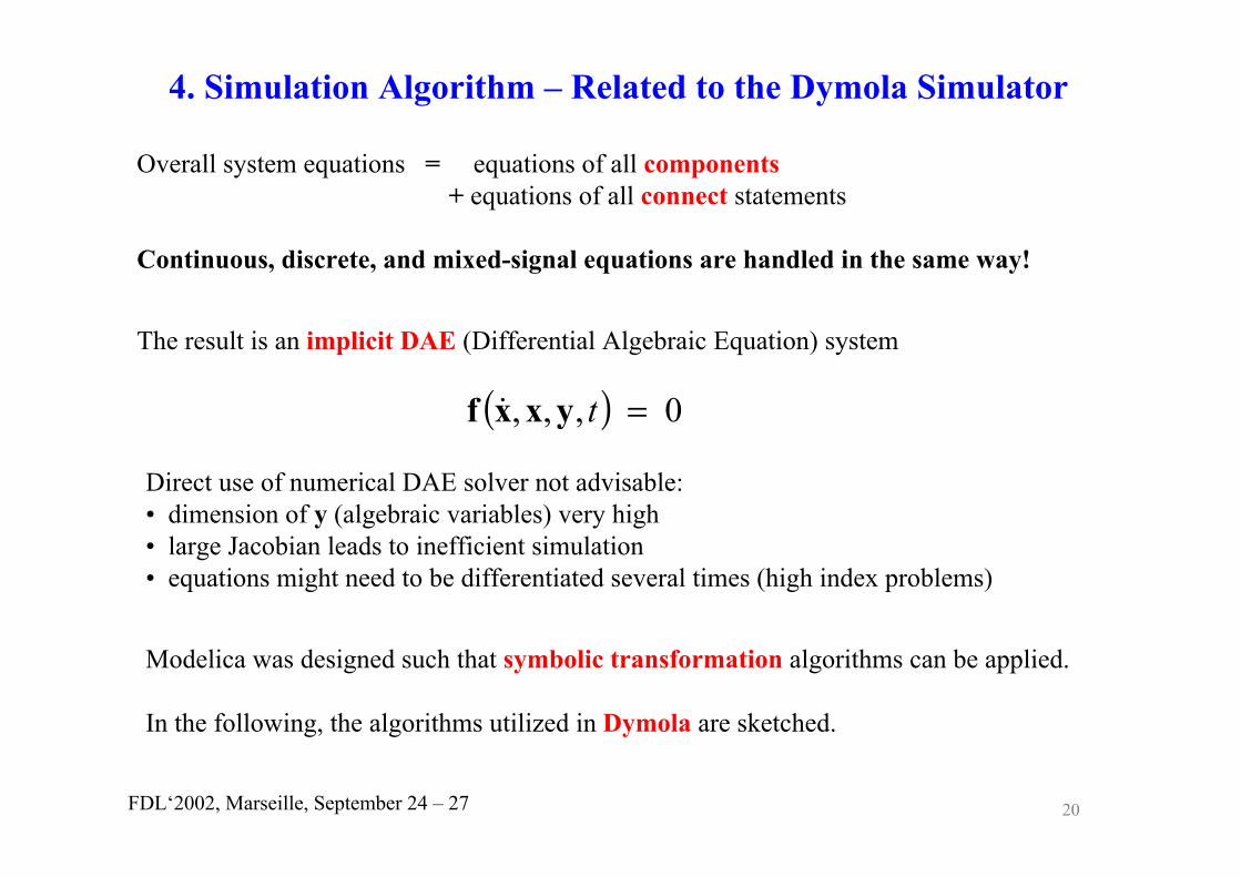
4. Simulation Algorithm – Related to the Dymola Simulator
Overall system equations = equations of all components+ equations of all connect statements
Continuous, discrete, and mixed-signal equations are handled in the same way!
The result is an implicit DAE (Differential Algebraic Equation) system
( ) 0,,, =tyxxf &
Direct use of numerical DAE solver not advisable:• dimension of y (algebraic variables) very high• large Jacobian leads to inefficient simulation • equations might need to be differentiated several times (high index problems)
Modelica was designed such that symbolic transformation algorithms can be applied.
In the following, the algorithms utilized in Dymola are sketched.

21FDL‘2002, Marseille, September 24 – 27
What Dymola Symbolic Solver Does for You:
• Transforms equations to efficient C-code• Sorts and equations• Solves equations symbolically (for reducing their number)• Solves or generates code for algebraic loops• Generates code to handle events• Generates symbolic Jacobians for efficient nonlinear iterations• Handles DAE with constraints (high index DAE’s)• Automatically assigns state variables• Generates code for consistent initialization of DAE
Dymola Symbolic SolverSimulator

22FDL‘2002, Marseille, September 24 – 27
Simulator Dymola
Output
Dymola simulation
C text
symbolical processing
graphical/textual input
OutputOutputOutput
Modelica text

23FDL‘2002, Marseille, September 24 – 27
model rlc Modelica.Electrical.Analog.Basic.Ground Ground1;Modelica.Electrical.Analog.Basic.Resistor R(R=100);Modelica.Electrical.Analog.Basic.Capacitor C;Modelica.Electrical.Analog.Basic.Inductor L;
equationconnect (C.n, L.n);connect (L.n, R.n);connect (C.p, L.p);connect (L.p, R.p);connect (C.p, Ground1.p);
end rlc;
Simulator Dymola
Output
Dymola simulation
C text
symbolical processing
graphical/textual input
OutputOutputOutputOutput
Modelica text
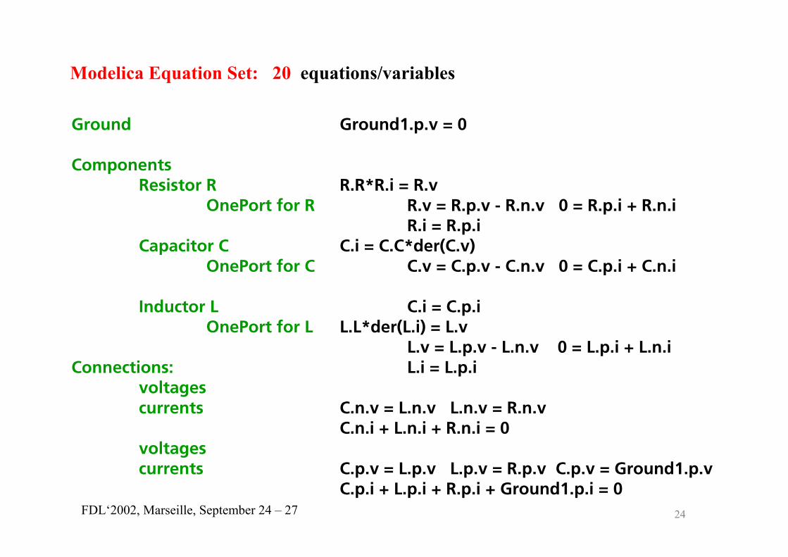
24FDL‘2002, Marseille, September 24 – 27
Ground
ComponentsResistor R
OnePort for R
Capacitor COnePort for C
Inductor LOnePort for L
Connections:voltages currents
voltagescurrents
Ground1.p.v = 0
R.R*R.i = R.v R.v = R.p.v - R.n.v 0 = R.p.i + R.n.iR.i = R.p.i
C.i = C.C*der(C.v)C.v = C.p.v - C.n.v 0 = C.p.i + C.n.i
C.i = C.p.iL.L*der(L.i) = L.v
L.v = L.p.v - L.n.v 0 = L.p.i + L.n.iL.i = L.p.i
C.n.v = L.n.v L.n.v = R.n.v C.n.i + L.n.i + R.n.i = 0
C.p.v = L.p.v L.p.v = R.p.v C.p.v = Ground1.p.vC.p.i + L.p.i + R.p.i + Ground1.p.i = 0
Modelica Equation Set: 20 equations/variables
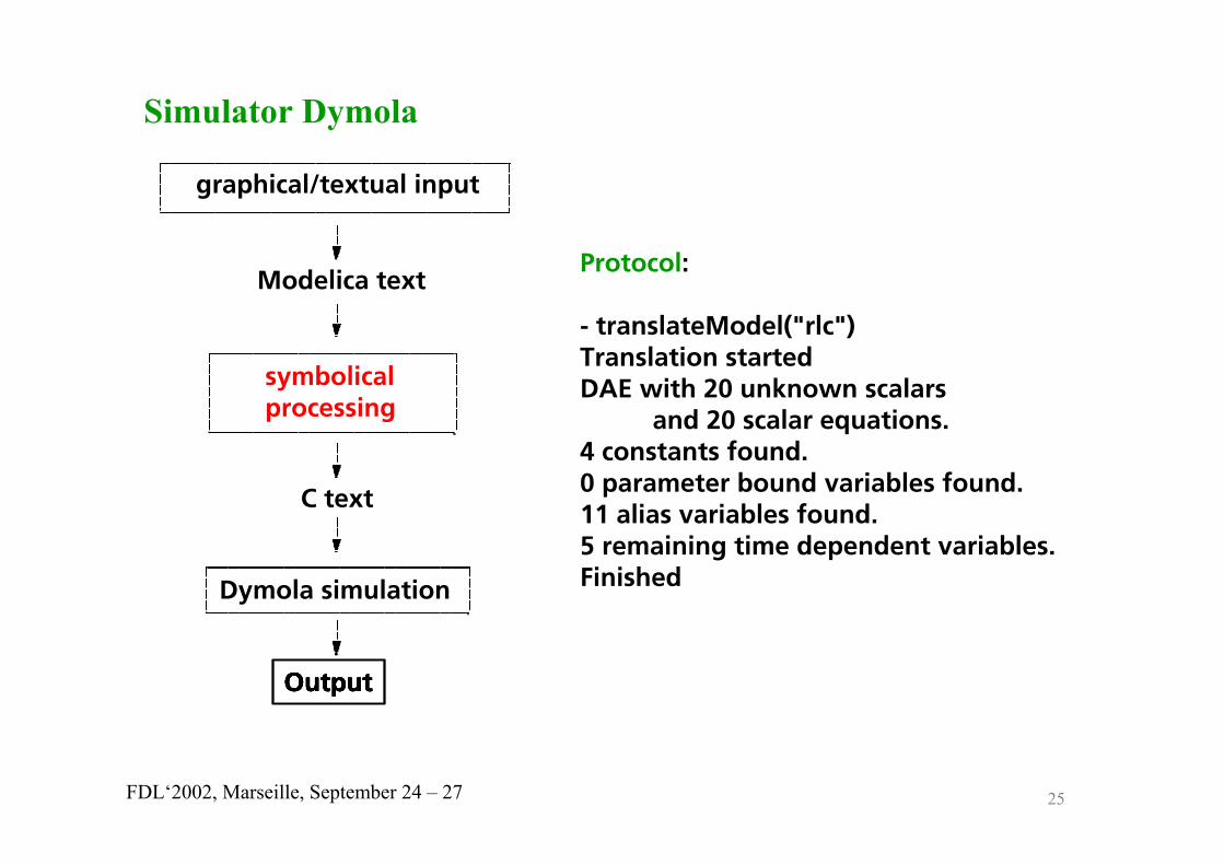
25FDL‘2002, Marseille, September 24 – 27
Protocol:
- translateModel("rlc")Translation startedDAE with 20 unknown scalars
and 20 scalar equations.4 constants found.0 parameter bound variables found.11 alias variables found.5 remaining time dependent variables.Finished
Simulator Dymola
Output
Dymola simulation
C text
symbolical processing
Modelica text
graphical/textual input
OutputOutputOutputOutput

26FDL‘2002, Marseille, September 24 – 27
Ground
ComponentsResistor R
OnePort for R
Capacitor COnePort for C
Inductor LOnePort for L
Connections:voltages currents
voltagescurrents
Ground1.p.v = 0
R.p.i = C.v / R.R R.v = R.p.v - R.n.v 0 = R.p.i + R.n.iR.i = R.p.i
der(C.v) = C.p.i / C.CC.v = C.p.v - C.n.v C.p.i = - (L.i + R.p.i)
C.i = C.p.ider(L.i) = C.v / L.L
L.v = L.p.v - L.n.v 0 = L.p.i + L.n.iL.i = L.p.i
C.n.v = L.n.v L.n.v = R.n.v C.n.i + L.n.i + R.n.i = 0
C.p.v = L.p.v L.p.v = R.p.v C.p.v = Ground1.p.vGround1.p.i = - (C.p.i + L.p.i + R.p.i)
Modelica Equation Set: 5 equations/variables

27FDL‘2002, Marseille, September 24 – 27
Ground
ComponentsResistor R
OnePort for R
Capacitor COnePort for C
Inductor LOnePort for L
Connections:voltages currents
voltagescurrents
Ground1.p.v = 0
R.R*R.i = R.v R.v = R.p.v - R.n.v 0 = R.p.i + R.n.iR.i = R.p.i
C.i = C.C*der(C.v)C.v = C.p.v - C.n.v 0 = C.p.i + C.n.i
C.i = C.p.iL.L*der(L.i) = C.v
L.v = L.p.v - L.n.v 0 = L.p.i + L.n.iL.i = L.p.i
C.n.v = L.n.v L.n.v = R.n.vC.C*der(C.v) + L.i + C.v / R.R
C.p.v = L.p.v L.p.v = R.p.v C.p.v = Ground1.p.vC.p.i + L.p.i + R.p.i + Ground1.p.i = 0
Modified Nodal Analysis Equation Set: 2 equations/variables

28FDL‘2002, Marseille, September 24 – 27
/* DSblock model generated by Dymola ... */#include .../* DSblock C-code: */ .../* Define variable names. */#define Sections_#define Ground1_p_v Variable(0)#define Ground1_p_i Variable(1)#define R_p_v Variable(2)#define L_L Parameter(2) ....
TranslatedEquations ....DynamicsSectionL_der_i = divmacro(C_v,"C.v",L_L,"L.L");R_p_i = divmacro(C_v,"C.v",R_R,"R.R");C_p_i = -(L_i+R_p_i);C_der_v = divmacro(C_p_i,"C.p.i",C_C,"C.C");
Ground1_p_i = -(C_p_i+L_i+R_p_i);EndTranslatedEquations ...
Simulator Dymola
Dymola simulation
C text
symbolical processing
Modelica text
graphical/textual input
Output

29FDL‘2002, Marseille, September 24 – 27
- experiment StopTime=500 NumberOfIntervals=5000- C.v := 5 ;- simulate--------------------------------------------------------------------------Log-file of program .\dymosim(generated: Fri May 03 08:49:01 2002)
dymosim started ...Integration started at T = 0 using integration method DASSL(DAE multi-step solver (dassl/dasslrt of Petzold
modified by Dynasim))Integration terminated successfully at T = 500
CPU-time for integration : 0.13 secondsCPU-time for one GRID interval: 0.026 milli-secondsNumber of result points : 5001Number of GRID points : 5001Number of (successful) steps : 3355Number of F-evaluations : 6733Number of Jacobian-evaluations: 17Number of (model) time events : 0Number of (U) time events : 0
Simulator Dymola
Output
Dymola simulation
C text
symbolical processing
Modelica text
graphical/textual input
OutputOutputOutputOutput

30FDL‘2002, Marseille, September 24 – 27
Simulator Dymola
Dymola simulation
C text
symbolical processing
Modelica text
graphical/textual input
Output

31FDL‘2002, Marseille, September 24 – 27
Two basic ideas for simulation acceleration:
1. New method “mixed mode integration” for real time simulation of systems which have “slow” and “fast” states:
- Slow states xS are discretized with the explicit Euler method.
- Fast states xF are discretized with the implicit Euler method.
2. Discretization formulae are inserted into model („inline integration“) and overall systems of equations are symbolically solved with Dymolas algorithmsto reduce the non-linear system and to generate analytical Jacobians !
Fn
Fn
Fn
Sn
Sn
Sn
nnnn
hh
t
xxx
xxx
yxxf0
&
&
&
⋅+=
⋅+=
=
−
−−
1
11
),,,(
• Local implicit small systems of equations• Automatic procedure for partitioning• Speed-up of 4 (diesel engine) ... 15 (detailed robot model).
Real-time simulation of stiff systems
slow
fast

32FDL‘2002, Marseille, September 24 – 27
5. Modelica librariesModelica Standard Library ( Modelica Association)
Electrical sublibraryBlock sublibraryRotational sublibraryTranslational sublibraryConstantsMathematical functionsSI unit types
HyLibLight Hydraulic Systems (Beater)ObjectStab ModelicaAdditions Library (DLR)Power Systems (Larsson) ExtendedPetriNetSystemDynamicsFuzzyControlATplus (Building simulation and control)Thermo fluid systems (Tummescheit)Electrical motors (Beuschel)Thermal systems (Tiller and DLR)PQLib (power quality analysis in networks)

33FDL‘2002, Marseille, September 24 – 27
Only commercially available:HyLib Hydraulic Systems – full version (Beater)PowerTrain (DLR) Fuel Cells (DLR)Thermal Building Behavior (U Kaiserslautern)Cooling and Heating Systems (U Hamburg-Harburg)TechThermo (DLR)Mass Flow in Process Plants (Zurich)Hybrid Electric Vehicles (U Gothenburg)Tyre Model Library (Royal Institute of Technology, S)Flight Dynamics Library (DLR)
Actual information:http://www.Modelica.org/libraries.html
Modelica libraries (cont’d)

34FDL‘2002, Marseille, September 24 – 27
Modelica.Thermal.Lumped
Modelica libraries (cont’d)

35FDL‘2002, Marseille, September 24 – 27
Modelica.Electrical.Analog
Modelica libraries (cont’d)

36FDL‘2002, Marseille, September 24 – 27
Modelica.Electrical.Analog.Basic
Modelica libraries (cont’d)

37FDL‘2002, Marseille, September 24 – 27
Modelica libraries (cont’d)
Modelica.Electrical.Analog.Ideal
38FDL‘2002, Marseille, September 24 – 27
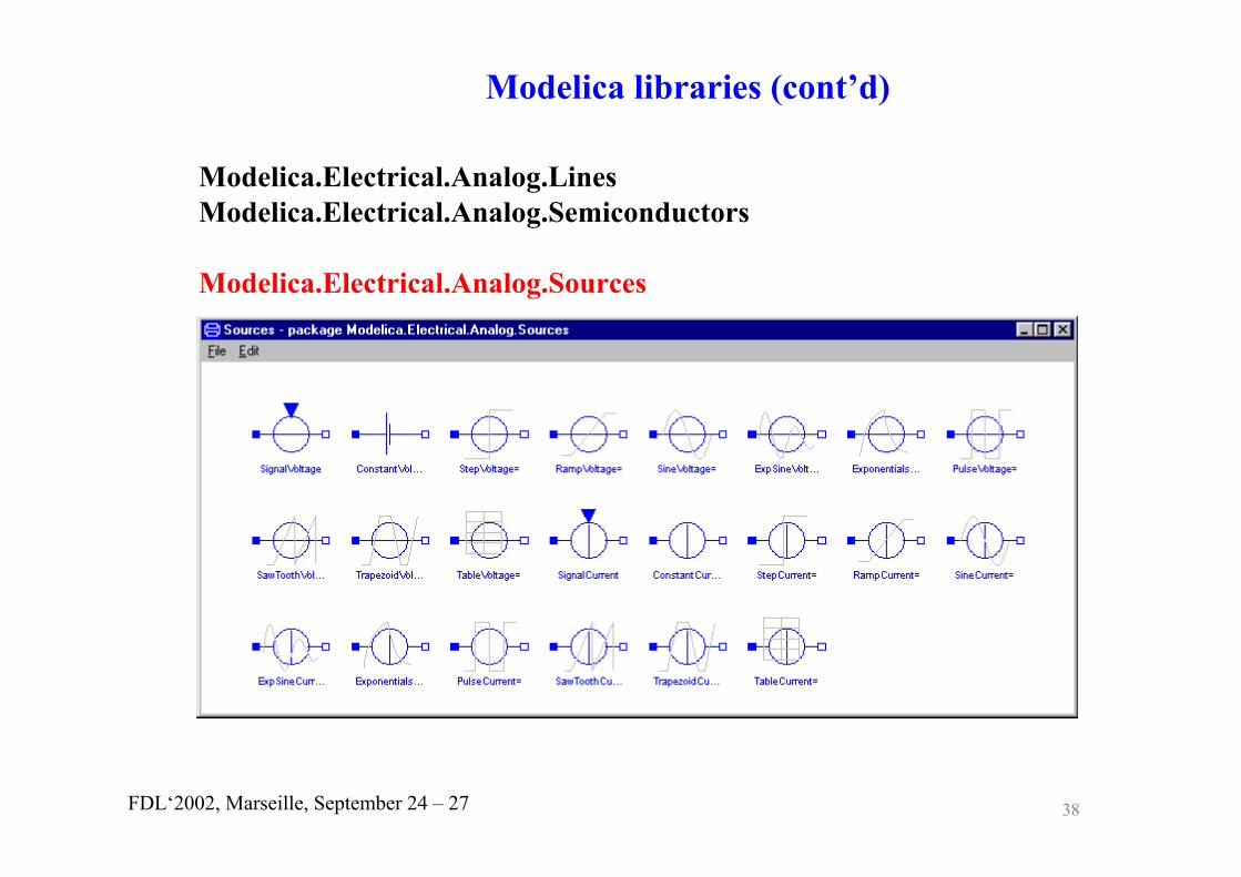
Modelica libraries (cont’d)
Modelica.Electrical.Analog.LinesModelica.Electrical.Analog.Semiconductors
Modelica.Electrical.Analog.Sources

39FDL‘2002, Marseille, September 24 – 27
6. Application Examples

40FDL‘2002, Marseille, September 24 – 27
model Resistorextends OnePort;parameter Real R;
equationv = R*i;
end Resistor;
Example: Industrial robot (DLR, Dynasim, KUKA)
1000 nontrivial algebraic equations, 80 states.With “mixed-mode integration”:
faster as real time on 650 Mhz PC.

41FDL‘2002, Marseille, September 24 – 27
Example: hardware-in-the-loop simulation of automatic gearbox(various car manufacturers)
Electronic Control Unit(Hardware)
+ driver + motor + torque converter + 1D vehicle dynamics
desired clutch pressure
(Simulation)

42FDL‘2002, Marseille, September 24 – 27
Example: Large, detailed vehicle model (Ford Motors, Dynasim, DLR)
• ~ 250.000 equations before reduction
• ~ 25.000 nontrival algebraic equations
• 320 states
3D-Mechanics (60 joints, 70 bodies)
Motor (combustion)
Power train (automatic gear box)
Hydraulics

43FDL‘2002, Marseille, September 24 – 27
Example: Material Testing Machine (U Paderborn, FhG EAS)
Hydraulic machine, controlled by an electronic circuit
Number of Equations/Variables
before aftersymbolic reduction
total 1.031 487
without electronics 309 137

44FDL‘2002, Marseille, September 24 – 27
Different controller models tested, here: operational amplifier
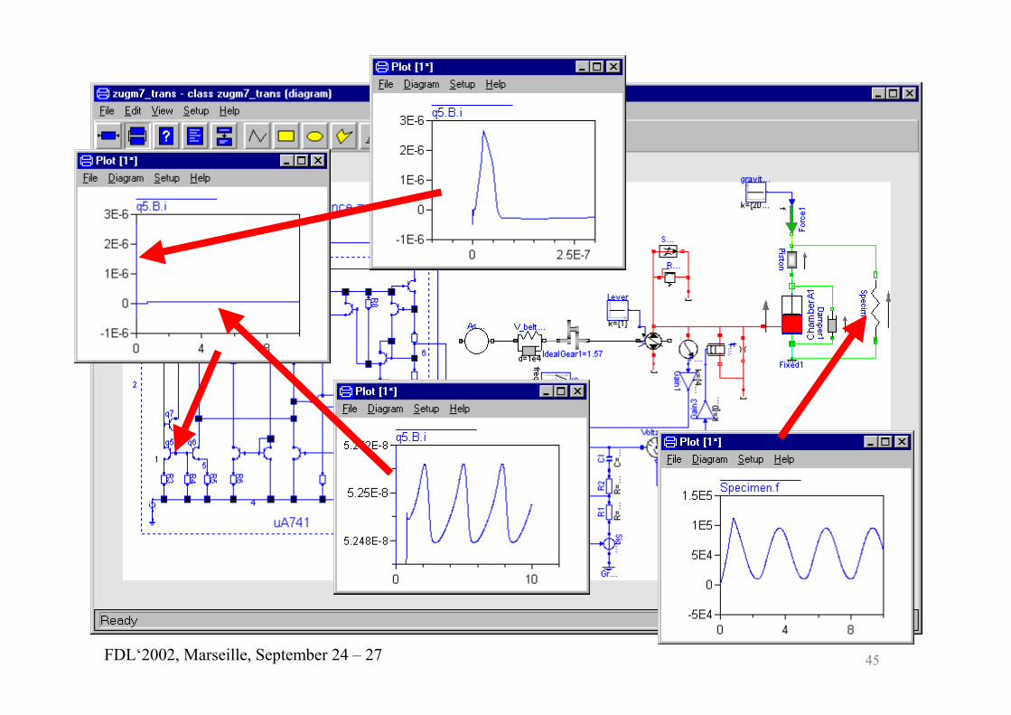
45FDL‘2002, Marseille, September 24 – 27

46FDL‘2002, Marseille, September 24 – 27
7. Comparison: VHDL-AMS and ModelicaDifferences Modelica VHDL-AMS
Origin Control systems, mechatronics Electronics, IC’s
Simulation modes TR, DC TR, DC, AC, Steady-State, Noise
Netlists Components, connection of pins, Components, nodes nodes not explicitely used
Graphics Annotations (for Docum., icons) (via EDA-tools)
Compact data like MATLAB-Syntax, matrices Operator overloading
Model change Composition, configuration, Composition, configuration inheritance
Digital time scale Digital event at any time possible Minimal resolvable time
Delays Not yet elaborated Precisely defined ( MVL9, ... )
Structure of model Cut set law explicitely to formulate Defines internal branches
User’s training For experts of object oriented For VHDL experts: easy to learnlanguages: easy to learn
Graphical input: very simple

47FDL‘2002, Marseille, September 24 – 27
8. Conclusion
• Modelica/Dymola is well suited to model large parts of the physical components,such as 3-dim. vehicle dynamics, power train including automatic gearboxes, hydraulics, combustion, electric/electronics, air conditioning, etc.
• Matlab/Simulink is well suited for signal-flow oriented components (control system / state charts and for the technical infra-structure: download to signal processors / Real Time Workshop; many toolboxes).
• Combination of Modelica and Simulink is very attractive(Dymola can generate Simulink CMEX S-Function of Modelica models).
• VHDL-AMS (e.g. VeriasHDL and AdvanceMS) is very powerful for electronicsubsystems, but perhaps not so strong for other parts of a complex systems, such as 3-dim. mechanics, power train, combustion, ... (lack of libraries!).
• Modelica/Dymola is especially suited for real-time simulation, such ashardware-in-the-loop (HIL); VHDL-AMS/RT in preparation.
• Modelica is supported by many multi-domain libraries, VHDL-AMS by large digital (and, in future, analog electrical) libraries; SPICE compatibility in analog electronics!
How to model and simulate heterogeneous systems?