Problems & Solutions - caos.fs.usb.vecaos.fs.usb.ve/libros/Statistical_Physics/Kardar, M -...
184
Problems & Solutions for Statistical Physics of Fields Updated July 2008 by Mehran Kardar Department of Physics Massachusetts Institute of Technology Cambridge, Massachusetts 02139, USA
Transcript of Problems & Solutions - caos.fs.usb.vecaos.fs.usb.ve/libros/Statistical_Physics/Kardar, M -...

Problems & Solutions
for
Statistical Physics of Fields
Updated July 2008
by
Mehran Kardar
Department of Physics
Massachusetts Institute of Technology
Cambridge, Massachusetts 02139, USA

Table of Contents
1. Collective Behavior, From Particles to Fields . . . . . . . . . . . . . . . . 1
2. Statistical Fields . . . . . . . . . . . . . . . . . . . . . . . . . . . . 18
3. Fluctuations . . . . . . . . . . . . . . . . . . . . . . . . . . . . . . 31
4. The Scaling Hypothesis . . . . . . . . . . . . . . . . . . . . . . . . . 55
5. Perturbative Renormalization Group . . . . . . . . . . . . . . . . . . . 63
6. Lattice Systems . . . . . . . . . . . . . . . . . . . . . . . . . . . . . 90
7. Series Expansions . . . . . . . . . . . . . . . . . . . . . . . . . . 106
8. Beyond Spin Waves . . . . . . . . . . . . . . . . . . . . . . . . . . 132

Solutions to problems from chapter 1- Collective Behavior, From Particles to Fields
1. The binary alloy: A binary alloy (as in β brass) consists of NA atoms of type A, and
NB atoms of type B. The atoms form a simple cubic lattice, each interacting only with its
six nearest neighbors. Assume an attractive energy of −J (J > 0) between like neighbors
A−A and B −B, but a repulsive energy of +J for an A−B pair.
(a) What is the minimum energy configuration, or the state of the system at zero temper-
ature?
• The minimum energy configuration has as little A-B bonds as possible. Thus, at zero
temperature atoms A and B phase separate, e.g. as indicated below.
A B
(b) Estimate the total interaction energy assuming that the atoms are randomly distributed
among the N sites; i.e. each site is occupied independently with probabilities pA = NA/N
and pB = NB/N .
• In a mixed state, the average energy is obtained from
E = (number of bonds) × (average bond energy)
= 3N ·(
−Jp2A − Jp2
B + 2JpApB
)
= −3JN
(
NA −NB
N
)2
.
(c) Estimate the mixing entropy of the alloy with the same approximation. Assume
NA, NB ≫ 1.
• From the number of ways of randomly mixing NA and NB particles, we obtain the
mixing entropy of
S = kB ln
(
N !
NA!NB!
)
.
Using Stirling’s approximation for large N (lnN ! ≈ N lnN−N), the above expression can
be written as
S ≈ kB (N lnN −NA lnNA −NB lnNB) = −NkB (pA ln pA + pB ln pB) .
1
(d) Using the above, obtain a free energy function F (x), where x = (NA−NB)/N . Expand
F (x) to the fourth order in x, and show that the requirement of convexity of F breaks
down below a critical temperature Tc. For the remainder of this problem use the expansion
obtained in (d) in place of the full function F (x).
• In terms of x = pA − pB , the free energy can be written as
F = E − TS
= −3JNx2 +NkBT
(
1 + x
2
)
ln
(
1 + x
2
)
+
(
1 − x
2
)
ln
(
1 − x
2
)
.
Expanding about x = 0 to fourth order, gives
F ≃ −NkBT ln 2 +N
(
kBT
2− 3J
)
x2 +NkBT
12x4.
Clearly, the second derivative of F ,
∂2F
∂x2= N (kBT − 6J) +NkBTx
2,
becomes negative for T small enough. Upon decreasing the temperature, F becomes
concave first at x = 0, at a critical temperature Tc = 6J/kB.
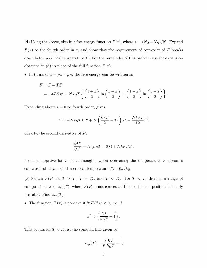
(e) Sketch F (x) for T > Tc, T = Tc, and T < Tc. For T < Tc there is a range of
compositions x < |xsp(T )| where F (x) is not convex and hence the composition is locally
unstable. Find xsp(T ).
• The function F (x) is concave if ∂2F/∂x2 < 0, i.e. if
x2 <
(
6J
kBT− 1
)
.
This occurs for T < Tc, at the spinodal line given by
xsp (T ) =
√
6J
kBT− 1,
2

T>Tc
T=Tc
T<Tc
T=0
F(x)/NJ
x+1-1
xsp(T)
as indicated by the dashed line in the figure below.
(f) The alloy globally minimizes its free energy by separating into A rich and B rich phases
of compositions ±xeq(T ), where xeq(T ) minimizes the function F (x). Find xeq(T ).
• Setting the first derivative of dF (x) /dx = Nx
(kBT − 6J) + kBTx2/3
, to zero yields
the equilibrium value of
xeq (T ) =
±√
3
√
6J
kBT− 1 for T < Tc
0 for T > Tc
.
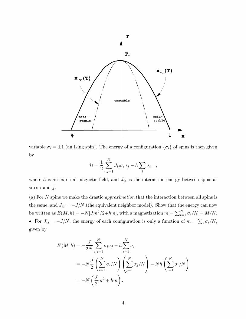
(g) In the (T, x) plane sketch the phase separation boundary ±xeq(T ); and the so called
spinodal line ±xsp(T ). (The spinodal line indicates onset of metastability and hysteresis
effects.)
• The spinodal and equilibrium curves are indicated in the figure above. In the interval
between the two curves, the system is locally stable, but globally unstable. The formation
of ordered regions in this regime requires nucleation, and is very slow. The dashed area is
locally unstable, and the system easily phase separates to regions rich in A and B.
********
2. The Ising model of magnetism: The local environment of an electron in a crystal
sometimes forces its spin to stay parallel or anti-parallel to a given lattice direction. As
a model of magnetism in such materials we denote the direction of the spin by a single
3
x1ÿ1
T
Tc
xeq(T)
x sp(T)
unstable
meta-stable
meta-stable
variable σi = ±1 (an Ising spin). The energy of a configuration σi of spins is then given
by
H =1
2
N∑
i,j=1
Jijσiσj − h∑
i
σi ;
where h is an external magnetic field, and Jij is the interaction energy between spins at
sites i and j.
(a) For N spins we make the drastic approximation that the interaction between all spins is
the same, and Jij = −J/N (the equivalent neighbor model). Show that the energy can now
be written as E(M,h) = −N [Jm2/2+hm], with a magnetizationm =∑N
i=1 σi/N = M/N .
• For Jij = −J/N , the energy of each configuration is only a function of m =∑
i σi/N ,
given by
E (M,h) = − J
2N
N∑
i,j=1
σiσj − h
N∑
i=1
σi
= −N J
2
(
N∑
i=1
σi/N
)
N∑
j=1
σj/N
−Nh
(
N∑
i=1
σi/N
)
= −N(
J
2m2 + hm
)
.
4

(b) Show that the partition function Z(h, T ) =∑
σi exp(−βH) can be re-written as
Z =∑
M exp[−βF (m, h)]; with F (m, h) easily calculated by analogy to problem (1). For
the remainder of the problem work only with F (m, h) expanded to 4th order in m.
• Since the energy depends only on the number of up spins N+, and not on their config-
uration, we have
Z (h, T ) =∑
σiexp (−βH)
=
N∑
N+=0
(number of configurations with N+ fixed) · exp [−βE (M,h)]
=N∑
N+=0
[
N !
N+! (N −N+)!
]
exp [−βE (M,h)]
=N∑
N+=0
exp
−β[
E (M,h) − kBT ln
(
N !
N+! (N −N+)!
)]
=∑
M
exp [−βF (m, h)] .
By analogy to the previous problem (N+ ↔ NA, m↔ x, J/2 ↔ 3J),
F (m, h)
N= −kBT ln 2 − hm+
1
2(kBT − J)m2 +
kBT
12m4 + O
(
m5)
.
(c) By saddle point integration show that the actual free energy F (h, T ) = −kT lnZ(h, T )
is given by F (h, T ) = min[F (m, h)]m. When is the saddle point method valid? Note that
F (m, h) is an analytic function but not convex for T < Tc, while the true free energy
F (h, T ) is convex but becomes non-analytic due to the minimization.
• Let m∗ (h, T ) minimize F (m, h), i.e. min [F (m, h)]m = F (m∗, h). Since there are N
terms in the sum for Z, we have the bounds
exp (−βF (m∗, h)) ≤ Z ≤ N exp (−βF (m∗, h)) ,
or, taking the logarithm and dividing by −βN ,
F (m∗, h)N
≥ F (h, T )
N≥ F (m∗, h)
N+
lnN
N.
5

Since F is extensive, we have therefore
F (m∗, h)N
=F (h, T )
N
in the N → ∞ limit.
(d) For h = 0 find the critical temperature Tc below which spontaneous magnetization
appears; and calculate the magnetization m(T ) in the low temperature phase.
• From the definition of the actual free energy, the magnetization is given by
m = − 1
N
∂F (h, T )
∂h,
i.e.
m = − 1
N
dF (m, h)
dh= − 1
N
∂F (m, h)
∂h+∂F (m, h)
∂m
∂m
∂h
.
Thus, if m∗ minimizes F (m, h), i.e. if ∂F (m, h)/∂m|m∗ = 0, then
m = − 1
N
∂F (m, h)
∂h
∣
∣
∣
∣
m∗
= m∗.
For h = 0,
m∗2 =3 (J − kBT )
kBT,
yielding
Tc =J
kB,
and
m =
±√
3 (J − kBT )
kBTif T < Tc
0 if T > Tc
.
(e) Calculate the singular (non-analytic) behavior of the response functions
C =∂E
∂T
∣
∣
∣
∣
h=0
, and χ =∂m
∂h
∣
∣
∣
∣
h=0
.
• The hear capacity is given by
C =∂E
∂T
∣
∣
∣
∣
h=0,m=m∗
= −NJ2
∂m∗2
∂T=
3NJTc
2T 2if T < Tc
0 if T > Tc
,
6

i.e. α = 0, indicating a discontinuity. To calculate the susceptibility, we use
h = (kBT − J)m+kBT
3m3.
Taking a derivative with respect to h,
1 =(
kBT − J + kBTm2) ∂m
∂h,
which gives
χ =∂m
∂h
∣
∣
∣
∣
h=0
=
1
2kB (Tc − T )if T < Tc
1
kB (T − Tc)if T > Tc
.
From the above expression we obtain γ± = 1, and A+/A− = 2.
********
3. The lattice–gas model: Consider a gas of particles subject to a Hamiltonian
H =
N∑
i=1
~pi2
2m+
1
2
∑
i,j
V(~ri − ~rj), in a volume V.
(a) Show that the grand partition function Ξ can be written as
Ξ =
∞∑
N=0
1
N !
(
eβµ
λ3
)N ∫ N∏
i=1
d3~ri exp
−β2
∑
i,j
V(~ri − ~rj)
.
• The grand partition function is calculated as
Ξ =
∞∑
N=0
eNβµ
N !ZN
=
∞∑
N=0
eNβµ
N !
∫ N∏
i=1
d3pid3ri
h3e−βH
=
∞∑
N=0
eNβµ
N !
(
N∏
i=1
∫
d3pi
h3e−βp2
i /2m
)
∫ N∏
i=1
d3ri exp
−β2
∑
i,j
Vij
=∞∑
N=0
1
N !
(
eNβ
λ3
)N ∫ N∏
i=1
d3ri exp
−β2
∑
i,j
Vij
,
7

where λ−1 =√
2πmkBT/h.
(b) The volume V is now subdivided into N = V/a3 cells of volume a3, with the spacing a
chosen small enough so that each cell α is either empty or occupied by one particle; i.e. the
cell occupation number nα is restricted to 0 or 1 (α = 1, 2, · · · ,N ). After approximating
the integrals∫
d3~r by sums a3∑N
α=1, show that
Ξ ≈∑
nα=0,1
(
eβµa3
λ3
)
∑
αnα
exp
−β2
N∑
α,β=1
nαnβV(~rα − ~rβ)
.
• Since
∫ N∏
i=1
d3ri exp
−β2
∑
i,j
Vij
≈ a3N′∑
exp
−β2
N∑
α,β=1
nαnβV (~rα − ~rβ)
·N !,
where the primed sum is over the configurations nα = 0, 1 with fixed N , and
N =N∑
α=1
nα,
we have
Ξ ≈∑
nα=0,1
(
eβµa3
λ3
)
∑
αnα
exp
−β2
N∑
α,β=1
nαnβV (~rα − ~rβ)
.
(c) By setting nα = (1 + σα)/2 and approximating the potential by V(~rα − ~rβ) = −J/N ,
show that this model is identical to the one studied in problem (2). What does this imply
about the behavior of this imperfect gas?
• With nα = (1 + σα) /2, and V (~rα − ~rβ) = −J/N ,
Ξ =∑
nα=0,1exp
(
βµ+ 3 lna
λ
)
N∑
α=1
(
1 + σα
2
)
+βJ
2NN∑
α,β=1
(
1 + σα
2
)(
1 + σβ
2
)
.
Setting m ≡ ∑
α σα/N , h′ = 12
(
µ+ 3β ln a
λ + J2
)
, and J ′ = J/4, the grand partition
function is written
Ξ = const.∑
nα=0,1exp
Nβ(
J ′m2/2 + h′m)
.
8

The phase diagram of the lattice-gas can thus be mapped onto the phase diagram of the
Ising model of problem 2. In particular, at a chemical potential µ such that h′ = 0, there
is a continuous “condensation” transition at a critical temperature Tc = J/4kB. (Note
that
m =∑
α
σα/N =∑
α
(2nα − 1) /N = 2a3ρ− 1,
where ρ = N/V is the density of the gas.)
• The manifest equivalence between these three systems is a straightforward consequence
of their mapping onto the same (Ising) Hamiltonian. However, there is a more subtle
equivalence relating the critical behavior of systems that cannot be so easily mapped onto
each other due to the Universality Principle.
********
4. Surfactant condensation: N surfactant molecules are added to the surface of water
over an area A. They are subject to a Hamiltonian
H =
N∑
i=1
~pi2
2m+
1
2
∑
i,j
V(~ri − ~rj),
where ~ri and ~pi are two dimensional vectors indicating the position and momentum of
particle i.
(a) Write down the expression for the partition function Z(N, T,A) in terms of integrals
over ~ri and ~pi, and perform the integrals over the momenta.
• The partition function is obtained by integrating the Boltzmann weight over phase space,
as
Z(N, T,A) =
∫∏N
i=1 d2~pid
2~qiN !h2N
exp
−βN∑
i=1
p2i
2m− β
∑
i<j
V(~qi − ~qj)
,
with β = 1/(kBT ). The integrals over momenta are simple Gaussians, yielding
Z(N, T,A) =1
N !
1
λ2N
∫ N∏
i=1
d2~qi exp
−β∑
i<j
V(~qi − ~qj)
,
where as usual λ = h/√
2πmkBT denotes the thermal wavelength.
The inter–particle potential V(~r) is infinite for separations |~r | < a, and attractive for
|~r | > a such that∫∞
a2πrdrV(r) = −u0.
9

(b) Estimate the total non–excluded area available in the positional phase space of the
system of N particles.
• To estimate the joint phase space of particles with excluded areas, add them to the
system one by one. The first one can occupy the whole area A, while the second can
explore only A − 2Ω, where Ω = πa2. Neglecting three body effects (i.e. in the dilute
limit), the area available to the third particle is (A− 2Ω), and similarly (A− nΩ) for the
n-th particle. Hence the joint excluded volume in this dilute limit is
A(A− Ω)(A− 2Ω) · · · (A− (N − 1)Ω) ≈ (A−NΩ/2)N ,
where the last approximation is obtained by pairing terms m and (N −m), and ignoring
order of Ω2 contributions to their product.
(c) Estimate the total potential energy of the system, assuming a uniform density n = N/A.
Using this potential energy for all configurations allowed in the previous part, write down
an approximation for Z.
• Assuming a uniform density n = N/A, an average attractive potential energy, U , is
estimated as
U =1
2
∑
i,j
Vattr.(~qi − ~qj) =1
2
∫
d2~r1d2~r2n(~r1)n(~r2)Vattr.(~r1 − ~r2)
≈n2
2A
∫
d2~r Vattr.(~r ) ≡ −N2
2Au0.
Combining the previous results gives
Z(N, T,A) ≈ 1
N !
1
λ2N(A−NΩ/2)N exp
[
βu0N2
2A
]
.
(d) The surface tension of water without surfactants is σ0, approximately independent of
temperature. Calculate the surface tension σ(n, T ) in the presence of surfactants.
• Since the work done is changing the surface area is dW = σdA, we have dF = −TdS +
σdA + µdN , where F = −kBT lnZ is the free energy. Hence, the contribution of the
surfactants to the surface tension of the film is
σs = − ∂ lnZ
∂A
∣
∣
∣
∣
T,N
= − NkBT
A−NΩ/2+u0N
2
2A2,
10

which is a two-dimensional variant of the familiar van der Waals equation. Adding the
(constant) contribution in the absence of surfactants gives
σ(n, T ) = σ0 −∂ lnZ
∂A
∣
∣
∣
∣
T,N
= − NkBT
A−NΩ/2+u0N
2
2A2.
(e) Show that below a certain temperature, Tc, the expression for σ is manifestly incorrect.
What do you think happens at low temperatures?
• Thermodynamic stability requires δσδA ≥ 0, i.e. σ must be a monotonically increasing
function of A at any temperature. This is the case at high temperatures where the first
term in the equation for σs dominates, but breaks down at low temperatures when the term
from the attractive interactions becomes significant. The critical temperature is obtained
by the usual conditions of ∂σs/∂A = ∂2σs/∂A2 = 0, i.e. from
∂σs
∂A
∣
∣
∣
∣
T
=NkBT
(A−NΩ/2)2− u0N
2
A3= 0
∂2σs
∂A2
∣
∣
∣
∣
T
= − 2NkBT
(A −NΩ/2)3+
3u0N2
A4= 0
,
The two equations are simultaneously satisfied for Ac = 3NΩ/2, at a temperature
Tc =8u0
27kBΩ.
As in the van der Waals gas, at temperatures below Tc, the surfactants separate into a
high density (liquid) and a low density (gas) phase.
(f) Compute the heat capacities, CA and write down an expression for Cσ without explicit
evaluation, due to the surfactants.
• The contribution of the surfactants to the energy of the film is given by
Es = −∂ lnZ
∂β= 2N × kBT
2− u0N
2
2A.
The first term is due to the kinetic energy of the surfactants, while the second arises from
their (mean-field) attraction. The heat capacities are then calculated as
CA =dQ
dT
∣
∣
∣
∣
A
=∂E
∂T
∣
∣
∣
∣
A
= NkB,
11

and
Cσ =dQ
dT
∣
∣
∣
∣
σ
=∂E
∂T
∣
∣
∣
∣
σ
− σ∂A
∂T
∣
∣
∣
∣
σ
.
********
5. Critical behavior of a gas: The pressure P of a gas is related to its density n = N/V ,
and temperature T by the truncated expansion
P = kBTn− b
2n2 +
c
6n3 ,
where b and c are assumed to be positive, temperature independent constants.
(a) Locate the critical temperature Tc below which this equation must be invalid, and
the corresponding density nc and pressure Pc of the critical point. Hence find the ratio
kBTcnc/Pc.
• Mechanical stability of the gas requires that any spontaneous change in volume should be
opposed by a compensating change in pressure. This corresponds to δPδV < 0, and since
δn = −(N/V 2)δV , any equation of state must have a pressure that is an increasing func-
tion of density. The transition point between pressure isotherms that are monotonically
increasing functions of n, and those that are not (hence manifestly incorrect) is obtained
by the usual conditions of dP/dn = 0 and d2P/dn2 = 0. Starting from the cubic equation
of state, we thus obtaindP
dn=kBTc − bnc +
c
2n2
c = 0
d2P
dn2= − b+ cnc = 0
.
From the second equation we obtain nc = b/c, which substituted in the first equation
gives kBTc = b2/(2c). From the equation of state we then find Pc = b3/(6c2), and the
dimensionless ratio ofkBTcnc
Pc= 3.
(b) Calculate the isothermal compressibility κT = − 1V
∂V∂P
∣
∣
T, and sketch its behavior as a
function of T for n = nc.
• Using V = N/n, we get
κT (n) = − 1
V
∂V
∂P
∣
∣
∣
∣
T
=1
n
∂P
∂n
∣
∣
∣
∣
−1
T
=[
n(
kBT − bn+ cn2/2)]−1
.
12

For n = nc, κT (nc) ∝ (T − Tc)−1, and diverges at Tc.
(c) On the critical isotherm give an expression for (P − Pc) as a function of (n− nc).
• Using the coordinates of the critical point computed above, we find
P − Pc = − b3
6c2+b2
2cn− b
2n2 +
c
6n3
=c
6
(
n3 − 3b
cn2 + 3
b2
c2n− b3
c3
)
=c
6(n− nc)
3.
(d) The instability in the isotherms for T < Tc is avoided by phase separation into a liquid
of density n+ and gas of density n−. For temperatures close to Tc, these densities behave
as n± ≈ nc (1 ± δ). Using a Maxwell construction, or otherwise, find an implicit equation
for δ(T ), and indicate its behavior for (Tc − T ) → 0. (Hint: Along an isotherm, variations
of chemical potential obey dµ = dP/n.)
• According to the Gibbs–Duhem relation, the variations of the intensive variables are
related by SdT − V dP + Ndµ = 0, and thus along an isotherm (dT = 0) dµ = dP/n =
∂P/∂n|Tdn/n. Since the liquid and gas states are in coexistence they should have the
same chemical potential. Integrating the above expression for dµ from n− to n+ leads to
the so-called Maxwell construction, which reads
0 = µ(n+) − µ(n−) =
∫ n+
n−
dP
n=
∫ nc(1+δ)
nc(1−δ)
dn
(
kBT − bn+ cn2/2
n
)
.
Performing the integrals gives the equation
0 = kBT ln
(
1 + δ
1 − δ
)
− bnc(2δ) +c
4n2
c
[
(1 + δ)2 − (1 − δ)2]
= kBT ln
(
1 + δ
1 − δ
)
− 2kBTcδ,
where for the find expression, we have used nc = b/c and kBTc = b2/(2c). The implicit
equation for δ is thus
δ =T
2Tcln
(
1 + δ
1 − δ
)
≈ T
Tc
(
δ − δ3 + · · ·)
.
The leading behavior as (Tc − T ) → 0 is obtained by keeping up to the cubic term, and
given by
δ ≈√
1 − Tc
T.
13

(e) Now consider a gas obeying Dieterici’s equation of state:
P (v − b) = kBT exp
(
− a
kBTv
)
,
where v = V/N . Find the ratio Pv/kBT at its critical point.
• The critical point is the point of inflection, described by
∂P
∂v
∣
∣
∣
∣
Tc,N
= 0, and∂2P
∂v2
∣
∣
∣
∣
Tc,N
= 0.
pres
sure
volume
1 2
4 3
coldQ
hot Qgasliq.
T
T-dT
P
P-dPV
The first derivative of P is
∂P
∂v
∣
∣
∣
∣
Tc,N
=∂
∂v
[
kBT
v − bexp
(
− a
kBTv
)]
=kBT
v − bexp
(
− a
kBTv
)(
a
kBTv2− 1
v − b
)
=P
(
a
kBTv2− 1
v − b
)
,
while a second derivative gives
∂2P
∂v2
∣
∣
∣
∣
Tc,N
=∂
∂v
[
P
(
a
kBTv2− 1
v − b
)]
=∂P
∂v
(
a
kBTv2− 1
v − b
)
− P
(
2a
kBTv3− 1
(v − b)2
)
.
Therefore vc and Tc are determined by
a
kBTcv2c
− 1
vc − b= 0, and
2a
kBTcv3c
− 1
(vc − b)2= 0,
14

with the solutions
vc = 2b, and kBTc =a
4b.
The critical pressure is
Pc =kBTc
vc − bexp
(
− a
kBTcvc
)
=a
4b2e−2,
resulting in the ratioPcvc
kBTc= 2e−2 ≈ 0.27.
Note that for the van der Waals gas
Pcvc
kBTc=
3
8= 0.375,
while for some actual gases
(
Pcvc
kBTc
)
water
= 0.230, and
(
Pcvc
kBTc
)
Argon
= 0.291.
(f) Calculate the isothermal compressibility κT for v = vc as a function of T − Tc for the
Dieterici gas.
• The isothermal compressibility is defined by
κT ≡ −1
v
∂v
∂P
∣
∣
∣
∣
T,N
,
and from part (a), given by
∂P
∂v
∣
∣
∣
∣
Tc,N
= P
(
a
kBTv2− 1
v − b
)
.
Expanding this expression, at v = vc, in terms of t ≡ kBT − kBTc (for T > Tc), yields
∂P
∂v
∣
∣
∣
∣
Tc,N
≈ Pc
(
a
(a/4b+ t) 4b2− 1
b
)
≈ −Pc
b
4bt
a= − 2Pc
vckBTct,
and thus
κT =kBTc
2Pc
1
t=
be2
2kB(T − Tc).
Note that expanding any analytic equation of state will yield the same simple pole for the
divergence of the compressibility.
15

(g) On the Dieterici critical isotherm expand the pressure to the lowest non-zero order in
(v − vc).
• Perform a Taylor–series expansion along the critical isotherm T = Tc, as
P (v, Tc) = Pc +∂P
∂v
∣
∣
∣
∣
Tc,vc
(v − vc) +1
2!
∂2P
∂v2
∣
∣
∣
∣
Tc,vc
(v − vc)2 +
1
3!
∂3P
∂v3
∣
∣
∣
∣
Tc,vc
(v − vc)3 + · · · .
The first two terms are zero at the critical point, and
∂3P
∂v3
∣
∣
∣
∣
Tc,vc
= −Pc∂
∂v
(
2a
kBTcv3− 1
(v − b)2
)
= −Pc
(
6a
kBTcv4c
− 2
(vc − b)3
)
= − Pc
2b3.
Substituting this into the Taylor expansion for P (v, Tc), results in
P (v, Tc) = Pc
(
1 − (v − vc)3
12b3
)
,
which is equivalent to
P
Pc− 1 =
2
3
(
v
vc− 1
)3
.
********
6. Magnetic thin films: A crystalline film (simple cubic) is obtained by depositing a
finite number of layers n. Each atom has a three component (Heisenberg) spin, and they
interact through the Hamiltonian
−βH =n∑
α=1
∑
<i,j>
JH~sαi · ~sα
j +n−1∑
α=1
∑
i
JV ~sαi · ~sα+1
i .
(The unit vector ~sαi indicates the spin at site i in the αth layer. The subscript < i, j >
indicates that the spin at i interacts with its 4 nearest-neighbors, indexed by j on the square
lattice on the same layer.) A mean–field approximation is obtained from the variational
density ρ0 ∝ exp (−βH0), with the trial Hamiltonian
−βH0 =n∑
α=1
∑
i
~hα · ~sαi .
16

(Note that the most general single–site Hamiltonian may include the higher order terms
Lαc1,···,cp
sαc1· · · sα
c1, where sc indicates component c of the vector ~s.)
(a) Calculate the partition function Z0
(
~hα)
, and βF0 = − lnZ0.
• The partition function Z0 is obtained by integrating over all angles as
Z0 =∏
i,α
[∫
d~sαi e
~h α·~s αi
]
=∏
i,α
[∫ 2π
0
dφ
∫ π
0
d cos θehα cos θ
]
=∏
i,α
[
2π
∫ 1
−1
dxehαx
]
=∏
i,α
[
2πehα − e−hα
hα
]
=
(
4π sinhhα
hα
)N
,
where N is the number of sites in each layer.
(b) Obtain the magnetizations mα =∣
∣〈~sαi 〉0∣
∣, and 〈βH0〉0, in terms of the Langevin func-
tion L(h) = coth(h) − 1/h.
• From the partition function, we easily obtain the magnetizations as
~mα = 〈~sαi 〉0 =
1
N
∂ lnZ0
∂~hα= hα ∂
∂hαln
sinhhα
hα= hα [cothhα − 1/hα] = hαL(hα).
(c) Calculate 〈βH〉0, with the (reasonable) assumption that all the variational fields(
~hα)
are parallel.
• For the zeroth order weight the spins at different sites are independent random variables,
and
〈βH〉0 = JH
n∑
α=1
∑
<i,j>
〈~sαi 〉0 ·
⟨
~sαj
⟩
0+ JV
n−1∑
α=1
∑
i
〈~sαi 〉0 ·
⟨
~sα+1i
⟩
0.
Noting that 〈~sαi 〉0 = mαh with all spins on average pointing in the same direction, and
that each spin has 4 neighbors in the plane on a square lattice, we obtain
〈βH〉0 = JH4N
2
n∑
α=1
mαmα + JV N
n−1∑
α=1
mαmα+1
= N
n∑
α=1
(
2JHm2α + JVmαmα+1
)
,
with mn+1 = 0.
17

(d) The exact free energy, βF = − lnZ, satisfies the Gibbs inequality (see below), βF ≤βF0 + 〈βH− βH0〉0. Give the self-consistent equations for the magnetizations mα that
optimize βH0. How would you solve these equations numerically?
• According to the Gibbs inequality βF ≤ NΨ(mα), with
Ψ(mα) =∑
α
[
− ln
(
4π sinhhα
hα
)
+ hαmα − 2JHm2α − JV mαmα+1
]
,
with mα = L(hα). The best variational choice for hα is obtained by minimizing Ψ, and
thus
∂Ψ
∂mα= −L(hα)
dhα
dmα+mα
dhα
dmα+ hα − 4JHmα − JV (mα+1 +mα−1) = 0.
After canceling the first two terms, the above equation can be re-written as
hα = L−1(mα) = 4JHmα + JV (mα+1 +mα−1) ,
which is the effective field acting on a site in layer α.
(e) Find the critical temperature, and the behavior of the magnetization in the bulk by
considering the limit n→ ∞. (Note that limm→0 L−1(m) = 3m+ 9m3/5 + O(m5).)
• When examining the bulk, we can drop the index α, and using the expansion of L−1(m)
we obtain
3m+9
5m3 + · · · = (4JH + JV )m.
The condition for criticality is the equality of the linear terms, i.e. 4JH +2JV = 3. Setting
JH = JH/kBT , and JV = JV /kBT , this gives kBTc = (4JH + 2JV )/3. For T < Tc, we
have9
5m3 = 3
(
Tc
T− 1
)
≡ 3t, =⇒ m = ±√
5t/3,
i.e. the usual saddle-point exponent of β = 1/2 is recovered.
(f) By linearizing the self-consistent equations, show that the critical temperature of film
depends on the number of layers n, as kTc(n≫ 1) ≈ kTc(∞) − JV π2/(3n2).
• For a finite number of layers, the linearized recursion relations are
L−1(mα) = 3mα + O(m3) = 4JHmα + JV (mα+1 +mα−1) .
18

These equations have to be supplemented by boundary conditions m0 = mn+1 = 0. The
solution to the linearized equations takes the form
mα = µ sin
(
απ
n+ 1
)
,
which gives the profile of magnetization at the critical point. It can be checked that this
is a solution to the linearized equations, by noting that
3µ sin
(
απ
n+ 1
)
+ · · · = 4JHµ sin
(
απ
n+ 1
)
+ JV µ
[
sin
(
(α+ 1)π
n+ 1
)
+ sin
(
(α− 1)π
n+ 1
)]
= 4JHµ sin
(
απ
n+ 1
)
+ JV µ
[
2 sin
(
απ
n+ 1
)
cos
(
π
n+ 1
)]
.
Thus the linear terms match is
4JH + 2JV cos
(
π
n+ 1
)
= 3,
giving the critical temperature of the finite system as
kBTc(n) =
[
JH + 2JV cos
(
π
n+ 1
)]
/3 ≈ kBTc(∞) − π2Jv
3n2+ · · · ,
where the last expression is obtained by expanding the cosine for large n.
(g) Derive a continuum form of the self-consistent equations, and keep terms to cubic order
in m. Show that the resulting non-linear differential equation has a solution of the form
m(x) = mbulk tanh(kx). What circumstances are described by this solution?
• The continuum limit is obtained by replacing the discrete layer number α with a contin-
uous coordinate z, such that mα → m(x), and
(mα+1 +mα−1) ≈ 2m(x) +d2m
dx2+ · · · .
In this limit the discrete set of equations are replaced with the differential equation
(4JH + 2JV )m(x) + JVd2m
dx2+ · · · = 3m+
9
5m3 + · · · .
To get the profile of a large system close to criticality the leading terms included above are
sufficient. It is in general not possible to give closed form solutions to non-linear equations.
However, it is easy to check that m(x) = mbulk tanh(kx) satisfies this equation, using
dm
dx= mbulkk
(
1 − tanh2 kx)
, andd2m
dx2= −2mbulkk
2 tanh(kx)(
1 − tanh2 kx)
.
19

Substituting in the differential equation gives
(4JH + 2JV )mbulk tanh(kx) − 2mbulkk2JV
(
tanh kx− tanh3 kx)
= 3mbulk tanh(kx) +9
5m3
bulk tanh3 kx.
Since the equality must hold irrespective of x, we must equate the coefficients of tanh kx
and tanh3 kx at each point. From the terms of order tanh kx, we get
(4JH + 2JV ) − 2k2JV = 0, =⇒ k2 =3 − (4JH + 2JV )
2JV,
while at order of tanh3 kx, we get
m2bulk =
10
9k2JV =
5
9[3 − (4JH + 2JV )] .
The latter agrees with the bulk magnetization obtained earlier, validating the consistency
of this solution. This profile corresponds to a domain wall in the system, located at
x = 0, separating a down magnetized phase at x → −∞, and an up magnetized phase at
x→ +∞.
(h) How can the above solution be modified to describe a semi–infinite system? Obtain
the critical behaviors of the healing length λ ∼ 1/k.
• As a first approximation to a semi–infinite system, we can take one half of the above
solution, say for x > 0. The magnetization is small (almost zero) at the surface, and
recovers to the bulk value over a distance λ ∼ 1/k ∝ t−1/2. Note that the divergence of
the healing length is precisely the same as the bulk correlation length.
(i) Show that the magnetization of the surface layer vanishes as |T − Tc|.• A more accurate answer is obtained by noting that in the discrete system, the coupling
to neighboring layers comes from mα−1 + mα+1. For the equation at the surface layer,
we have m−1 +m1, and we must set m−1 = 0. Thus a more accurate solution is actually
shifted by one lattice spacing, as m(x ≥ 0) = mbulk tanh[k(x+ a)] for a lattice spacing a.
Expanding the tanh gives
m0 = msurface ≈ mbulkka ∝ t.
The result in (f) illustrates a quite general result that the transition temperature
of a finite system of size L, approaches its asymptotic (infinite–size) limit from below,
as Tc(L) = TC(∞) − A/L1/ν , where ν is the exponent controlling the divergence of the
correlation length. However, some liquid crystal films appeared to violate this behavior.
In fact, in these films the couplings are stronger on the surface layers, which thus order
before the bulk. For a discussion of the dependence of Tc on the number of layers in this
case, see H. Li, M. Paczuski, M. Kardar, and K. Huang, Phys. Rev. B 44, 8274 (1991).
********
20

Solutions to problems from chapter 2- Statistical Fields
1. Cubic invariants: When the order parameter m, goes to zero discontinuously, the
phase transition is said to be first order (discontinuous). A common example occurs in
systems where symmetry considerations do not exclude a cubic term in the Landau free
energy, as in
βH =
∫
ddx
[
K
2(∇m)2 +
t
2m2 + cm3 + um4
]
(K, c, u > 0).
(a) By plotting the energy density Ψ(m), for uniform m at various values of t, show that
as t is reduced there is a discontinuous jump to m 6= 0 for a positive t in the saddle–point
approximation.
• To simplify the algebra, let us rewrite the energy density Ψ(m), for uniform m, in terms
of the rescaled quantity
mr =u
cm.
In this way, we can eliminate the constant parameters c, and u, to get the expression of
the energy density as
Ψr(mr) =1
2trm
2r +m3
r +m4r,
where we have defined
Ψr =
(
c4
u3
)
Ψ, and tr =( u
c2
)
t.
To obtain the extrema of Ψr, we set the first derivative with respect to mr to zero, i.e.
dΨr(mr)
dmr= mr
(
tr + 3mr + 4m2r
)
= 0.
The trivial solution of this equation is m∗r = 0. But if tr ≤ 9/16, the derivative vanishes
also at m∗r = (−3 ± √
9 − 16tr)/8. Provided that tr > 0, m∗r = 0 is a minimum of the
function Ψr(mr). In addition, if tr < 9/16, Ψr(mr) has another minimum at
m∗r = −3 +
√9 − 16tr8
,
and a maximum, located in between the two minima, at
m∗r =
−3 +√
9 − 16tr8
.
21

Fr
m r
1 2 3 412
3
4
The accompanying figure depicts the behavior of Ψr(mr) for different values of tr.
1. For tr > 9/16, there is only one minimum m∗r = 0 .
2. For 0 < tr < tr < 9/16, there are two minima, but Ψr(m∗r) > Ψr(0) = 0.
3. For 0 < tr = tr, Ψr(m∗r) = Ψr(0) = 0.
4. For 0 < tr < tr, Ψr(m∗r) < Ψr(0) = 0.
The discontinuous transition occurs when the local minimum at m∗r < 0 becomes the
absolute minimum. There is a corresponding jump of mr, from m∗r = 0 to m∗
r = mr, where
mr = m∗r(tr = tr).
(b) By writing down the two conditions that m and t must satisfy at the transition, solve
for m and t.
• To determine mr and tr, we have to simultaneously solve the equations
dΨr(mr)
dmr= 0, and Ψr(mr) = Ψr(0) = 0.
Excluding the trivial solution m∗r = 0, from
tr + 3mr + 4m2r = 0
tr2
+mr +m2r = 0
,
we obtain tr = −mr = 1/2, or in the original units,
t =c2
2u, and m = − c
2u.
22

tt
ξ
ξ max
(c) Recall that the correlation length ξ is related to the curvature of Ψ(m) at its minimum
by Kξ−2 = ∂2Ψ/∂m2|eq.. Plot ξ as a function of t.
•Likewise, the equilibrium value of m = meq in the original units equals to
meq =
0 for t > t =c2
2u,
−( c
u
) 3 +√
9 − 16ut/c2
8for t < t.
The correlation length ξ, is related to the curvature of Ψ(m) at its equilibrium minimum
by
Kξ−2 =∂2Ψ
∂m2
∣
∣
∣
∣
meq
= t+ 6cmeq + 12um2eq,
which is equal to
ξ =
(
K
t
)1/2
if t > t,
(
− K
2t+ 3cmeq
)1/2
if t < t.
(To arrive to the last expression, we have useddΨ(m)/dm|m=meq= 0.)
ξmax = ξ(t) =
√2Ku
c.
23

A plot of ξ as a function of t is presented here. Note that the correlation length ξ, is finite
at the discontinuous phase transition, attaining a maximum value of
********
2. Tricritical point: By tuning an additional parameter, a second order transition can be
made first order. The special point separating the two types of transitions is known as a
tricritical point, and can be studied by examining the Landau–Ginzburg Hamiltonian
βH =
∫
ddx
[
K
2(∇m)2 +
t
2m2 + um4 + vm6 − hm
]
,
where u can be positive or negative. For u < 0, a positive v is necessary to ensure stability.
(a) By sketching the energy density Ψ(m), for various t, show that in the saddle–point
approximation there is a first-order transition for u < 0 and h = 0.
• If we consider h = 0, the energy density Ψ(m), for uniform m, is
Ψ(m) =t
2m2 + um4 + vm6.
As in the previous problem, to obtain the extrema of Ψ, let us set the first derivative with
respect to m to zero. Again, provided that t > 0, Ψ(m) has a minimum at m∗ = 0. But
the derivative also vanishes for other nonzero values of m as long as certain conditions are
satisfied. In order to find them, we have to solve the following equation
t+ 4um2 + 6vm4 = 0,
from which,
m∗2 = − u
3v±
√4u2 − 6tv
6v.
Thus, we have real and positive solutions provided that
u < 0, and t <2u2
3v.
Under these conditions Ψ(m) has another two minima at
m∗2 =|u|3v
+
√4u2 − 6tv
6v,
and two maxima at
m∗2 =|u|3v
−√
4u2 − 6tv
6v,
24

F
m
12
3
4
12
3
4
as depicted in the accompanying figure.
The different behaviors of the function Ψ(m) are as follows:
1. For t > 2u2/3v, there is only one minimum m∗ = 0.
2. For 0 < t < t < 2u2/3v, there are three minima, but Ψ(±m∗) > Ψ(0) = 0.
3. For 0 < t = t, Ψ(±m∗) = Ψ(0) = 0.
4. For 0 < t < t, Ψ(±m∗) < Ψ(0) = 0.
There is a thus discontinuous phase transition for u < 0, and t = t(u).
(b) Calculate t and the discontinuity m at this transition.
• To determine t, and m = m∗(t = t), we again have to simultaneously solve the equations
dΨ(m)
dm2= 0, and Ψ(m2) = Ψ(0) = 0,
or equivalently,
t
2+ 2um2 + 3vm4 = 0
t
2+ um2 + vm4 = 0
,
from which we obtain
t =u2
2v, and m2 = − u
2v=
|u|2v.
25

(c) For h = 0 and v > 0, plot the phase boundary in the (u, t) plane, identifying the phases,
and order of the phase transitions.
• In the (u, t) plane, the line t = u2/2v for u < 0, is a first-order phase transition
boundary. In addition, the line t = 0 for u > 0, defines a second-order phase transition
boundary, as indicated in the accompanying figure.
second orderboundary
disorderedphase
tricriticalpoint
ordered
phase
first orderboundary
t
u
(d) The special point u = t = 0, separating first– and second–order phase boundaries, is
a tricritical point. For u = 0, calculate the tricritical exponents β, δ, γ, and α, governing
the singularities in magnetization, susceptibility, and heat capacity. (Recall: C ∝ t−α;
m(h = 0) ∝ tβ ; χ ∝ t−γ ; and m(t = 0) ∝ h1/δ.)
• For u = 0, let us calculate the tricritical exponents α, β, γ, and δ. In order to calculate
α and β, we set h = 0, so that
Ψ(m) =t
2m2 + vm6.
Thus from∂Ψ
∂m
∣
∣
∣
∣
m
= m(
t+ 6vm4)
= 0,
26

we obtain,
m =
0 for t > t = 0,(
− t
6v
)1/4
for t < 0,
resulting in,
m(h = 0) ∝ tβ , with β =1
4.
The corresponding free energy density scales as
Ψ(m) ∼ m 6 ∝ (−t)3/2.
The tricritical exponent α characterizes the non-analytic behavior of the heat capacity
C ∼ (∂2Ψ/∂T 2)|h=0,m, and since t ∝ (T − Tc),
C ∼ ∂2Ψ
∂t2
∣
∣
∣
∣
h=0,m
∝ t−α, with α =1
2.
To calculate the tricritical exponent δ, we set t = 0 while keeping h 6= 0, so that
Ψ(m) = vm6 − hm.
Thus from∂Ψ
∂m
∣
∣
∣
∣
m
= 6vm5 − h = 0,
we obtain,
m ∝ h1/δ, with δ = 5.
Finally, for h 6= 0 and t 6= 0,
∂Ψ
∂m
∣
∣
∣
∣
m
= tm+ 6vm5 − h = 0,
so that the susceptibility scales as
χ =∂m
∂h
∣
∣
∣
∣
h=0
∝ |t|−1, for both t < 0 and t > 0,
i.e. with the exponents γ± = 1.
********
3. Transverse susceptibility: An n–component magnetization field ~m(x) is coupled to an
external field ~h through a term −∫
ddx ~h · ~m(x) in the Hamiltonian βH. If βH for ~h = 0
27

is invariant under rotations of ~m(x); then the free energy density (f = − lnZ/V ) only
depends on the absolute value of ~h; i.e. f(~h) = f(h), where h = |~h|.(a) Show that mα = 〈
∫
ddxmα(x)〉/V = −hαf′(h)/h.
• The magnetic work is the product of the magnetic field and the magnetization density,
and appears as the argument of the exponential weight in the (Gibbs) canonical ensemble.
We can thus can “lower” the magnetization M =∫
ddxmα (x) “inside the average” by
taking derivatives of the (Gibbs) partition function with respect to hα, as
mα =1
V
⟨∫
ddxmα (x)
⟩
=1
V
∫
Dm (x)(∫
ddx′mα (x′))
e−βH∫
Dm (x) e−βH
=1
V
1
Z
1
β
∂
∂hα
∫
Dm (x) e−βH =1
βV
∂
∂hαlnZ = − ∂f
∂hα.
For an otherwise rotationally symmetric system, the (Gibbs) free energy depends only on
the magnitude of h, and using
∂h
∂hα=∂√
hβhβ
∂hα=
1
2
2δαβhβ√
hβhβ
=hα
h,
we obtain
mα = − ∂f
∂hα= − df
dh
∂h
∂hα= −f ′hα
h.
(b) Relate the susceptibility tensor χαβ = ∂mα/∂hβ , to f ′′(h), ~m, and ~h.
• The susceptibility tensor is now obtained as
χαβ =∂mα
∂hβ=
∂
∂hβ
(
−hα
hf ′ (h)
)
= −∂hα
∂hβ
1
hf ′ − ∂h−1
∂hβhαf
′ − hα
h
∂f ′
∂hβ
= −(
δαβ − hαhβ
h2
)
f ′
h− hαhβ
h2f ′′.
In order to express f ′ in terms of the magnetization, we take the magnitude of the result
of part (a),
m = |f ′ (h)| = −f ′ (h) ,
from which we obtain
χαβ =
(
δαβ − hαhβ
h2
)
m
h+hαhβ
h2
dm
dh.
(c) Show that the transverse and longitudinal susceptibilities are given by χt = m/h and
χℓ = −f ′′(h); where m is the magnitude of ~m.
28

• Since the matrix(
δαβ − hαhβ/h2)
removes the projection of any vector along the mag-
netic field, we conclude
χℓ = −f ′′ (h) =dm
dh
χt =m
h
.
Alternatively, we can choose the coordinate system such that hi = hδi1 (i = 1, . . . , d), to
get
χℓ = χ11 =
(
δ11 −h1h1
h2
)
m
h− h1h1
h2f ′′ (h) =
dm
dh
χt = χ22 =
(
δ11 −h2h2
h2
)
m
h− h2h2
h2f ′′ (h) =
m
h
.
(d) Conclude that χt diverges as ~h → 0, whenever there is a spontaneous magnetization.
Is there any similar a priori reason for χℓ to diverge?
• Provided that limh→0m 6= 0, the transverse susceptibility clearly diverges for h → 0.
There is no similar reason, on the other hand, for the longitudinal susceptibility to diverge.
In the saddle point approximation of the Landau–Ginzburg model, for example, we have
tm+ 4um3 + h = 0,
implying (since 4um2 = −t at h = 0, for t < 0) that
χℓ|h=0 =
(
dh
dm
)−1∣
∣
∣
∣
∣
h=0
= (t− 3t)−1, i .e. χℓ =
1
2 |t| ,
at zero magnetic field, in the ordered phase (t < 0).
NOTE: Another, more pictorial approach to this problem is as follows. Since the Hamil-
tonian is invariant under rotations about h, m must be parallel to h, i.e.
mα =hα
hϕ (h) ,
where ϕ is some function of the magnitude of the magnetic field. For simplicity, let h = he1,
with e1 a unit vector, implying that
m = me1 = ϕ (h) e1.
The longitudinal susceptibility is then calculated as
χℓ =∂m1
∂h1
∣
∣
∣
∣
h=he1
=dm
dh= ϕ′ (h) .
29

To find the transverse susceptibility, we first note that if the system is perturbed by a
small external magnetic field δhe2, the change in m1 is, by symmetry, the same for δh > 0
and δh < 0, implying
m1 (he1 + δhe2) = m1 (he1) + O(
δh2)
.
Hence∂m1
∂h2
∣
∣
∣
∣
h=he1
= 0.
Furthermore, since m and h are parallel,
m1 (he1 + δhe2)
h=m2 (he1 + δhe2)
δh,
from which
m2 (he1 + δhe2) =m1 (he1)
hδh+ O
(
δh3)
,
yielding
χt =∂m2
∂h2
∣
∣
∣
∣
h=he1
=m
h.
********
4. Superfluid He4–He3 mixtures: The superfluid He4 order parameter is a complex
number ψ(x) . In the presence of a concentration c(x) of He3 impurities, the system has
the following Landau–Ginzburg energy
βH[ψ, c] =
∫
ddx
[
K
2|∇ψ|2 +
t
2|ψ|2 + u |ψ|4 + v |ψ|6 +
c(x)2
2σ2− γc(x)|ψ|2
]
,
with positive K, u and v.
(a) Integrate out the He3 concentrations to find the effective Hamiltonian, βHeff [ψ], for
the superfluid order parameter, given by
Z =
∫
Dψ exp (−βHeff [ψ]) ≡∫
DψDc exp (−βH[ψ, c]) .
• The integration over c(x) is merely a Gaussian integral, which at each point gives
∫
dc(x) exp
(
−c(x)2
2σ2+ γc(x)|ψ|2
)
∝ exp
(
+1
2γ2σ2|ψ|4
)
.
30

This modifies the quartic term in the Hamiltonian, resulting in
−βHeff [ψ] =
∫
ddx
[
K
2|∇ψ|2 +
t
2|ψ|2 +
(
u− γ2σ2
2
)
|ψ|4 + v |ψ|6]
.
(b) Obtain the phase diagram for βHeff [ψ] using a saddle point approximation. Find the
limiting value of σ∗ above which the phase transition becomes discontinuous.
• As long as the quartic term is positive, in the saddle point approximation there is a
continuous phase transition at t = 0, separating a disordered phase for t > 0, and a
superfluid phase for t < 0. The fourth order term becomes negative for σ > σ∗ =√
2u/γ,
and the phase transition is then discontinuous.
(c) The discontinuous transition is accompanied by a jump in the magnitude of ψ. How
does this jump vanish as σ → σ∗?
• The saddle point solution minimizes the above energy, leading to
tψ + 4uψ 3 + 6vψ 5 = 0,
where u = u− γ2σ2/2 ∝ (σ∗ − σ). At the first order boundary, the resulting energy must
equal to that of the disordered phase with ψ = 0, resulting in a second equation
t
2ψ 2 + uψ 4 + vψ 6 = 0.
Eliminating t between the above two equations gives
ψ 2 = − u
2v∝ (σ − σ∗) ,
i.e. the discontinuity in ψ along the boundary vanishes as√σ − σ∗.
(d) Show that the discontinuous transition is accompanied by a jump in He3 concentration.
• From the initial Gaussian Hamiltonian for c(x), it is easy to see that
〈c(x)〉 = γσ2|ψ|2.
Hence a discontinuity in ψ is necessarily accompanied by a discontinuity in the density
c(x). (Note that the ensemble for He3 is grand canonical, thus allowing this change in
density.)
(e) Sketch the phase boundary in the (t, σ) coordinates, and indicate how its two segments
join at σ∗.
31

t
Normal Fluid
Superfluid
s* s
• Using the above value of Ψ2
in one of the equations determining the transition point,
one finds
t = −4
(
u− σ2γ2
2
)
Ψ2 − 6vΨ
4=γ4
8v
(
σ2 − σ∗2)2 ,
i.e. the discontinuous line joins the continuous portion quadratically, as illustrated in the
figure
(f) Going back to the original joint probability for the fields c(x) and Ψ(x), show that
〈c(x) − γσ2|Ψ(x)|2〉 = 0.
• By grouping the quadratic forms involving c(x), the joint probability can be written as
e−βH = e−∫
ddx
[
K2 |∇Ψ|2+ t
2 |Ψ|2+(
u−σ2γ2
2
)
|Ψ|4+v|Ψ|6+ (c(x)−γσ2|Ψ(x)|2)2
2σ2
]
.
We can change variables to c′(x) = c(x) − γσ2|Ψ(x)|2, whose average is clearly zero by
symmetry, and hence
〈c(x)〉 = γσ2〈|Ψ(x)|2〉.
(g) Show that 〈c(x)c(y)〉 = γ2σ4〈|Ψ(x)|2|Ψ(y)|2〉, for x 6= y.
• Since the field c′(x) is not coupled to any other field at a different location in space,
〈c′(x)c′(y)〉 = 0, and 〈c′(x)|Ψ(y)2|〉 = 0. Hence,
〈c(x)c(y)〉 = 〈(
c′(x) + γσ2|Ψ(x)|2) (
c′(y) + γσ2|Ψ(y)|2)
〉 = γ2σ4〈|Ψ(x)|2|Ψ(y)|2〉.
(h) Qualitatively discuss how 〈c(x)c(0)〉 decays with x = |x| in the disordered phase.
32

• In the disordered phase 〈Ψ(x)Ψ(0)〉 decays exponentially, as e−x/ξ . From the result of
the previous part, we expect
〈c(x)c(0)〉 ∼ γ2σ4 exp
(
−2x
ξ
)
.
(i) Qualitatively discuss how 〈c(x)c(0)〉 decays to its asymptotic value in the ordered phase.
• In the ordered phase, 〈Ψ(x)Ψ(0)〉 ∼ 1/xd−2 due to the Goldstone mode. Hence in d = 3
dimensions,
〈c(x)c(0)〉 ∼ 1/x2.
********
5. Crumpled surfaces: The configurations of a crumpled sheet of paper can be described
by a vector field ~r(x), denoting the position in three dimensional space, ~r = (r1, r2, r3), of
the point at location x = (x1, x2) on the flat sheet. The energy of each configuration is
assumed to be invariant under translations and rotations of the sheet of paper.
(a) Show that the two lowest order (in derivatives) terms in the quadratic part of a Landau–
Ginzburg Hamiltonian for this system are:
βH0[~r] =∑
α=1,2
∫
d2x
[
t
2∂α~r · ∂α~r +
K
2∂2
α~r · ∂2α~r
]
.
• Since the energy in the sheet is invariant under translations, it cannot depend on
the vector ~r, but only on its gradients such as ∂α~r, and ∂α∂β~r. To ensure rotational
invariance, each component ri must be contracted (paired and summed over) with another
ri. Similarly to ensure isotropy in x = (x1, x2), each derivative ∂α must be paired with
another one. Taking advantage of contractions is a good way to find invariants. Thus
using the summation notation, and ensuring proper contractions, the lowest order terms
in the effective Hamiltonian are
βH0[~r] =
∫
d2x
[
t
2∂αri∂αri +
K
2∂α∂αri∂β∂βri
]
.
(b) Write down the lowest order terms (there are two) that appear at the quartic level.
33

• The same procedure allows us to construct 4-th order terms in ~r: There should be two
ri, two rj and derivatives that are contracted. The two possible terms are
βH′[~r] =
∫
d2x [u∂αri∂αri∂βrj∂βrj + v∂αri∂βri∂αrj∂βrj ] .
(c) Discuss what happens when t changes sign, assuming that quartic terms provide the
required stability (and K > 0).
• The above theory has the same structure as the Landau-Ginzburg Hamiltonian, which
a more complicated order parameter (∂αri in place of mi). As in the Landau-Ginzburg
model, when t become negative, the order parameter is no longer zero, but the weight is
maximized for a finite value of ∂αri. This implies that the sheet of paper gets stretched
along a specific direction. This is known as the crumpling (or uncrumpling) transition.
The sheet of paper is in a crumpled state for t > 0, while for t < 0, it opens up in some
arbitrary direction.
********
34

Solutions to problems from chapter 3 - Fluctuations
1. Spin waves: In the XY model of n = 2 magnetism, a unit vector ~s = (sx, sy) (with
s2x + s2y = 1) is placed on each site of a d–dimensional lattice. There is an interaction that
tends to keep nearest–neighbors parallel, i.e. a Hamiltonian
−βH = K∑
<ij>
~si · ~sj .
The notation < ij > is conventionally used to indicate summing over all nearest–neighbor
pairs (i, j).
(a) Rewrite the partition function Z =∫∏
i d~si exp(−βH), as an integral over the set of
angles θi between the spins ~si and some arbitrary axis.
• The partition function is
Z =
∫
∏
i
d2~si exp
K∑
〈ij〉~si · ~sj
δ(
~si2 − 1
)
.
Since ~si · ~sj = cos (θi − θj), and d2~si = dsidθisi = dθi, we obtain
Z =
∫
∏
i
dθi exp
K∑
〈ij〉cos (θi − θj)
.
(b) At low temperatures (K ≫ 1), the angles θi vary slowly from site to site. In this
case expand −βH to get a quadratic form in θi.• Expanding the cosines to quadratic order gives
Z = eNbK
∫
∏
i
dθi exp
−K2
∑
〈ij〉(θi − θj)
2
,
where Nb is the total number of bonds. Higher order terms in the expansion may be
neglected for large K, since the integral is dominated by |θi − θj | ≈√
2/K.
(c) For d = 1, consider L sites with periodic boundary conditions (i.e. forming a closed
chain). Find the normal modes θq that diagonalize the quadratic form (by Fourier trans-
formation), and the corresponding eigenvalues K(q). Pay careful attention to whether the
modes are real or complex, and to the allowed values of q.
35

• For a chain of L sites, we can change to Fourier modes by setting
θj =∑
q
θ (q)eiqj
√L.
Since θj are real numbers, we must have
θ (−q) = θ (q)∗,
and the allowed q values are restricted, for periodic boundary conditions, by the require-
ment of
θj+L = θj , ⇒ qL = 2πn, with n = 0,±1,±2, . . . ,±L2.
Using
θj − θj−1 =∑
q
θ (q)eiqj
√L
(
1 − e−iq)
,
the one dimensional Hamiltonian, βH = K2
∑
j (θj − θj−1)2, can be rewritten in terms of
Fourier components as
βH =K
2
∑
q,q′
θ (q) θ (q′)∑
j
ei(q+q′)j
L
(
1 − e−iq)
(
1 − e−iq′)
.
Using the identity∑
j ei(q+q′)j = Lδq,−q′, we obtain
βH = K∑
q
|θ (q)|2 [1 − cos (q)] .
(d) Generalize the results from the previous part to a d–dimensional simple cubic lattice
with periodic boundary conditions.
• In the case of a d dimensional system, the index j is replaced by a vector
j 7→ j = (j1, . . . , jd) ,
which describes the lattice. We can then write
βH =K
2
∑
j
∑
α
(
θj − θj+eα
)2,
36

where eα’s are unit vectors e1 = (1, 0, · · · , 0) , · · · , ed = (0, · · · , 0, 1), generalizing the one
dimensional result to
βH =K
2
∑
q,q′
θ (q) θ (q′)∑
α
∑
j
ei(q+q′)·j
Ld
(
1 − e−iq·eα)
(
1 − e−iq′·eα
)
.
Again, summation over j constrains q and −q′ to be equal, and
βH = K∑
q
|θ (q)|2∑
α
[1 − cos (qα)] .
(e) Calculate the contribution of these modes to the free energy and heat capacity. (Eval-
uate the classical partition function, i.e. do not quantize the modes.)
• With K (q) ≡ 2K∑
α [1 − cos (qα)],
Z =
∫
∏
q
dθ (q) exp
[
−1
2K (q) |θ (q)|2
]
=∏
q
√
2π
K (q),
and the corresponding free energy is
F = −kBT lnZ = −kBT
[
constant − 1
2
∑
q
lnK (q)
]
,
or, in the continuum limit (using the fact that the density of states in q space is (L/2π)d),
F = −kBT
[
constant − 1
2Ld
∫
ddq
(2π)d
lnK (q)
]
.
As K ∼ 1/T at T → ∞, we can write
F = −kBT
[
constant′ +1
2Ld lnT
]
,
and the heat capacity per site is given by
C = −T ∂2F
∂T 2· 1
Ld=kB
2.
This is because there is one degree of freedom (the angle) per site that can store potential
energy.
37

(f) Find an expression for 〈~s0 · ~sx〉 = ℜ〈exp[iθx − iθ0]〉 by adding contributions from
different Fourier modes. Convince yourself that for |x| → ∞, only q → 0 modes contribute
appreciably to this expression, and hence calculate the asymptotic limit.
• We have
θx − θ0 =∑
q
θ (q)eiq·x − 1
Ld/2,
and by completing the square for the argument of the exponential in⟨
ei(θx−θ0)⟩
, i.e. for
−1
2K (q) |θ (q)|2 + iθ (q)
eiq·x − 1
Ld/2,
it follows immediately that
⟨
ei(θx−θ0)⟩
= exp
− 1
Ld
∑
q
∣
∣eiq·x − 1∣
∣
2
2K (q)
= exp
−∫
ddq
(2π)d
1 − cos (q · x)
K (q)
.
For x larger than 1, the integrand has a peak of height ∼ x2/2K at q = 0 (as it is
seen by expanding the cosines for small argument). Furthermore, the integrand has a first
node, as q increases, at q ∼ 1/x. From these considerations, we can obtain the leading
behavior for large x:
• In d = 1, we have to integrate ∼ x2/2K over a length ∼ 1/x, and thus
⟨
ei(θx−θ0)⟩
∼ exp
(
− |x|2K
)
.
• In d = 2, we have to integrate ∼ x2/2K over an area ∼ (1/x)2. A better approximation,
at large x, than merely taking the height of the peak, is given by
∫
ddq
(2π)d
1 − cos (q · x)
K (q)≈∫
dqdϕq
(2π)2
1 − cos (qx cosϕ)
Kq2
=
∫
dqdϕ
(2π)2
1
Kq−∫
dqdϕ
(2π)2
cos (qx cosϕ)
Kq,
or, doing the angular integration in the first term,
∫
ddq
(2π)d
1 − cos (q · x)
K (q)≈∫ 1/|x| dq
2π
1
Kq+ subleading in x,
resulting in⟨
ei(θx−θ0)⟩
∼ exp
(
− ln |x|2πK
)
= |x|− 12πK , as x→ ∞.
38

• In d ≥ 3, we have to integrate ∼ x2/2K over a volume ∼ (1/x)3. Thus, as x → ∞, the
x dependence of the integral is removed, and
⟨
ei(θx−θ0)⟩
→ constant,
implying that correlations don’t disappear at large x.
The results can also be obtained by noting that the fluctuations are important only for
small q. Using the expansion of K(q) ≈ Kq2/2, then reduces the problem to calculation
of the Coulomb Kernel∫
ddqeiq·x/q2, as described in the preceding chapter.
(g) Calculate the transverse susceptibility from χt ∝∫
ddx〈~s0 · ~sx〉c. How does it depend
on the system size L?
• We have⟨
ei(θx−θ0)⟩
= exp
−∫
ddq
(2π)d
1 − cos (q · x)
K (q)
,
and, similarly,⟨
eiθx⟩
= exp
−∫
ddq
(2π)d
1
2K (q)
.
Hence the connected correlation function
〈~sx · ~s0〉c =⟨
ei(θx−θ0)⟩
c=⟨
ei(θx−θ0)⟩
−⟨
eiθx⟩ ⟨
eiθ0⟩
,
is given by
〈~sx · ~s0〉c = e−∫
ddq
(2π)d1
K(q)
exp
[
∫
ddq
(2π)d
cos (q · x)
K (q)
]
− 1
.
In d ≥ 3, the x dependent integral vanishes at x→ ∞. We can thus expand its exponential,
for large x, obtaining
〈~sx · ~s0〉c ∼∫
ddq
(2π)d
cos (q · x)
K (q)≈∫
ddq
(2π)d
cos (q · x)
Kq2=
1
KCd(x) ∼
1
K |x|d−2.
Thus, the transverse susceptibility diverges as
χt ∝∫
ddx 〈~sx · ~s0〉c ∼L2
K.
(h) In d = 2, show that χt only diverges for K larger than a critical value Kc = 1/(4π).
39

• In d = 2, there is no long range order, 〈~sx〉 = 0, and
〈~sx · ~s0〉c = 〈~sx · ~s0〉 ∼ |x|−1/(2πK).
The susceptibility
χt ∼∫ L
d2x |x|−1/(2πK),
thus converges for 1/(2πK) > 2, for K below Kc = 1/(4π). For K > Kc, the susceptibility
diverges as
χt ∼ L2−2Kc/K .
********
2. Capillary waves: A reasonably flat surface in d–dimensions can be described by its
height h, as a function of the remaining (d − 1) coordinates x = (x1, ...xd−1). Convince
yourself that the generalized “area” is given by A =∫
dd−1x√
1 + (∇h)2. With a surface
tension σ, the Hamiltonian is simply H = σA.
(a) At sufficiently low temperatures, there are only slow variations in h. Expand the energy
to quadratic order, and write down the partition function as a functional integral.
• For a surface parametrized by the height function
xd = h (x1, . . . , xd−1) ,
an area element can be calculated as
dA =1
cosαdx1 · · ·dxd−1,
where α is the angle between the dth direction and the normal
~n =1
√
1 + (∇h)2
(
− ∂h
∂x1, . . . ,− ∂h
∂xd−1, 1
)
to the surface (n2 = 1). Since, cosα = nd =[
1 + (∇h)2]−1/2
≈ 1 − 12 (∇h)2, we obtain
H = σA ≈ σ
∫
dd−1x
1 +1
2(∇h)2
,
40

and, dropping a multiplicative constant,
Z =
∫
Dh (x) exp
−β σ2
∫
dd−1x (∇h)2
.
(b) Use Fourier transformation to diagonalize the quadratic Hamiltonian into its normal
modes hq (capillary waves).
• After changing variables to the Fourier modes,
h (x) =
∫
dd−1q
(2π)d−1
h (q) eiq·x,
the partition function is given by
Z =
∫
Dh (q) exp
−β σ2
∫
dd−1q
(2π)d−1
q2 |h (q)|2
.
(c) What symmetry breaking is responsible for these Goldstone modes?
• By selecting a particular height, the ground state breaks the translation symmetry in
the dth direction. The transformation h (x) → h (x) + ξ (x) leaves the energy unchanged
if ξ (x) is constant. By continuity, we can have an arbitrarily small change in the energy
by varying ξ (x) arbitrarily slowly.
(d) Calculate the height–height correlations 〈(
h(x) − h(x′))2〉.
• From
h (x) − h (x′) =
∫
dd−1q
(2π)d−1
h (q)(
eiq·x − eiq·x′)
,
we obtain
⟨
(h (x) − h (x′))2⟩
=
∫
dd−1q
(2π)d−1
dd−1q′
(2π)d−1
〈h (q) h (q′)〉(
eiq·x − eiq·x′)(
eiq′·x − eiq′·x′)
.
The height-height correlations thus behave as
G (x− x′) ≡⟨
(h (x) − h (x′))2⟩
=2
βσ
∫
dd−1q
(2π)d−1
1 − cos [q · (x − x′)]q2
=2
βσCd−1 (x − x′) .
(e) Comment on the form of the result (d) in dimensions d = 4, 3, 2, and 1.
41

• We can now discuss the asymptotic behavior of the Coulomb Kernel for large |x − x′|,either using the results from problem 1(f), or the exact form given in lectures.
• In d ≥ 4, G (x− x′) → constant, and the surface is flat.
• In d = 3, G (x − x′) ∼ ln |x − x′|, and we come to the surprising conclusion that there
are no asymptotically flat surfaces in three dimensions. While this is technically correct,
since the logarithm grows slowly, very large surfaces are needed to detect appreciable
fluctuations.
• In d = 2, G (x − x′) ∼ |x − x′|. This is easy to comprehend, once we realize that the
interface h(x) is similar to the path x(t) of a random walker, and has similar (x ∼√t)
fluctuations.
• In d = 1, G (x − x′) ∼ |x − x′|2. The transverse fluctuation of the ‘point’ interface are
very big, and the approximations break down as discussed next.
(f) By estimating typical values of ∇h, comment on when it is justified to ignore higher
order terms in the expansion for A.
• We can estimate (∇h)2 as
⟨
(h (x) − h (x′))2⟩
(x− x′)2∝ |x − x′|1−d
.
For dimensions d ≥ dℓ = 1, the typical size of the gradient decreases upon coarse-graining.
The gradient expansion of the area used before is then justified. For dimensions d ≤ dℓ,
the whole idea of the gradient expansion fails to be sensible.
********
3. Gauge fluctuations in superconductors: The Landau–Ginzburg model of supercon-
ductivity describes a complex superconducting order parameter Ψ(x) = Ψ1(x) + iΨ2(x),
and the electromagnetic vector potential ~A(x), which are subject to a Hamiltonian
βH =
∫
d3x
[
t
2|Ψ|2 + u|Ψ|4 +
K
2DµΨD∗
µΨ∗ +L
2(∇× A)
2
]
.
The gauge-invariant derivative Dµ ≡ ∂µ − ieAµ(x), introduces the coupling between the
two fields. (In terms of Cooper pair parameters, e = e∗c/h, K = h2/2m∗.)
(a) Show that the above Hamiltonian is invariant under the local gauge symmetry:
Ψ(x) 7→ Ψ(x) exp (iθ(x)) , and Aµ(x) 7→ Aµ(x) +1
e∂µθ.
42

• Under a local gauge transformation, βH 7−→∫
d3x
t
2|Ψ|2 + u |Ψ|4 +
K
2
[
(∂µ − ieAµ − i∂µθ)Ψeiθ] [
(∂µ + ieAµ + i∂µθ)Ψ∗e−iθ]
+L
2
(
∇× ~A+ ∇× 1
e∇θ)2
.
But this is none other than βH again, since
(∂µ − ieAµ − i∂µθ)Ψeiθ = eiθ (∂µ − ieAµ) Ψ = eiθDµΨ,
and
∇× 1
e∇θ = 0.
(b) Show that there is a saddle point solution of the form Ψ(x) = Ψ, and ~A(x) = 0, and
find Ψ for t > 0 and t < 0.
• The saddle point solutions are obtained from
δHδΨ∗ = 0, =⇒ t
2Ψ + 2uΨ |Ψ|2 − K
2DµDµΨ = 0,
andδHδAµ
= 0, =⇒ K
2
(
−ieΨD∗µΨ∗ + ieΨ∗DµΨ
)
− Lǫαβµǫαγδ∂β∂γAδ = 0.
The ansatz Ψ (x) = Ψ, ~A = 0, clearly solves these equations. The first equation then
becomes
tΨ + 4uΨ∣
∣Ψ∣
∣
2= 0,
yielding (for u > 0) Ψ = 0 for t > 0, whereas∣
∣Ψ∣
∣
2= −t/4u for t < 0.
(c) For t < 0, calculate the cost of fluctuations by setting
Ψ(x) =(
Ψ + φ(x))
exp (iθ(x)) ,
Aµ(x) = aµ(x), (with ∂µaµ = 0 in the Coulomb gauge)
and expanding βH to quadratic order in φ, θ, and ~a.
• For simplicity, let us choose Ψ to be real. From the Hamiltonian term
DµΨD∗µΨ∗ =
[
(∂µ − ieaµ)(
Ψ + φ)
eiθ] [
(∂µ + ieaµ)(
Ψ + φ)
e−iθ]
,
43

we get the following quadratic contribution
Ψ2(∇θ)2 + (∇φ)
2 − 2eΨ2aµ∂µθ + e2Ψ
2 |~a|2 .
The third term in the above expression integrates to zero (as it can be seen by integrating
by parts and invoking the Coulomb gauge condition ∂µaµ = 0). Thus, the quadratic terms
read
βH(2) =
∫
d3x
(
t
2+ 6uΨ
2)
φ2 +K
2(∇φ)
2+K
2Ψ
2(∇θ)2
+K
2e2Ψ
2 |~a|2 +L
2(∇× ~a)2
.
(d) Perform a Fourier transformation, and calculate the expectation values of⟨
|φ(q)|2⟩
,⟨
|θ(q)|2⟩
, and⟨
|~a(q)|2⟩
.
• In terms of Fourier transforms, we obtain
βH(2) =∑
q
(
t
2+ 6uΨ
2+K
2q2)
|φ (q)|2 +K
2Ψ
2q2 |θ (q)|2
+K
2e2Ψ
2 |~a (q)|2 +L
2(q × ~a)2
.
In the Coulomb gauge, q ⊥ ~a (q), and so [q× ~a (q)]2
= q2 |~a (q)|2. This diagonal form
then yields immediately (for t < 0)
⟨
|φ (q)|2⟩
=(
t+ 12uΨ2
+Kq2)−1
=1
Kq2 − 2t,
⟨
|θ (q)|2⟩
=(
KΨ2q2)−1
= − 4u
Ktq2,
⟨
|~a (q)|2⟩
= 2(
Ke2Ψ2
+ Lq2)−1
=2
Lq2 −Ke2t/4u(~a has 2 components).
Note that the gauge field, “mass-less” in the original theory, acquires a “mass” Ke2t/4u
through its coupling to the order parameter. This is known as the Higgs mechanism.
********
4. Fluctuations around a tricritical point: As shown in a previous problem, the Hamilto-
nian
βH =
∫
ddx
[
K
2(∇m)2 +
t
2m2 + um4 + vm6
]
,
44

with u = 0 and v > 0 describes a tricritical point.
(a) Calculate the heat capacity singularity as t→ 0 by the saddle point approximation.
• As already calculated in a previous problem, the saddle point minimum of the free
energy ~m = meℓ, can be obtained from
∂Ψ
∂m
∣
∣
∣
∣
m
= m(
t+ 6vm 4)
= 0,
yielding,
m =
0 for t > t = 0(
− t
6v
)1/4
for t < 0.
The corresponding free energy density equals to
Ψ(m) =t
2m 2 + vm 6 =
0 for t > 0
−1
3
(−t)3/2
(6v)1/2for t < 0
.
Therefore, the singular behavior of the heat capacity is given by
C = Cs.p. ∼ −Tc∂2Ψ
∂t2
∣
∣
∣
∣
m
=
0 for t > 0
Tc
4(−6vt)−1/2 for t < 0
,
as sketched in the figure below.
t
C
(b) Include both longitudinal and transverse fluctuations by setting
~m(x) =(
m+ φℓ(x))
eℓ +
n∑
α=2
φαt (x)eα,
45

and expanding βH to quadratic order in φ.
• Let us now include both longitudinal and transversal fluctuations by setting
~m(x) = (m+ φℓ(x))eℓ +
n∑
α=2
φαt (x)eα,
where eℓ and eα form an orthonormal set of n vectors. Consequently, the free energy βHis a function of φℓ and φt. Since meℓ is a minimum, there are no linear terms in the
expansion of βH in φ. The contributions of each factor in the free energy to the quadratic
term in the expansion are
(∇~m)2 =⇒ (∇φℓ)2 +
n∑
α=2
(∇φαt )2,
(~m)2 =⇒ (φℓ)2 +
n∑
α=2
(φαt )2,
(~m)6 = ((~m)2)3 = (m2 + 2mφℓ + φ2ℓ +
n∑
α=2
(φαt )2)3 =⇒ 15m 4(φℓ)
2 + 3m 4n∑
α=2
(φαt )2.
The expansion of βH to second order now gives
βH(φℓ, φαt ) = βH(0, 0) +
∫
ddx
[
K
2(∇φℓ)
2 +φ2
ℓ
2
(
t+ 30vm4)
]
+
n∑
α=2
[
K
2(∇φα
t )2 +(φα
t )2
2
(
t+ 6vm4)
]
.
We can formally rewrite it as
βH(φℓ, φαt ) = βH(0, 0) + βHℓ(φℓ) +
n∑
α=2
βHtα(φα
t ),
where βHi(φi), with i = ℓ, tα, is in general given by
βHi(φi) =K
2
∫
ddx
[
(∇φi)2 +
φ2i
ξ2i
]
,
with the inverse correlation lengths
ξ−2ℓ =
t
Kfor t > 0
−4t
Kfor t < 0
,
46

and
ξ−2tα
=
t
Kfor t > 0
0 for t < 0.
As shown in the lectures for the critical point of a magnet, for t > 0 there is no difference
between longitudinal and transverse components, whereas for t < 0, there is no restoring
force for the Goldstone modes φαt due to the rotational symmetry of the ordered state.
(c) Calculate the longitudinal and transverse correlation functions.
• Since in the harmonic approximation βH turns out to be a sum of the Hamiltonians
of the different fluctuating components φℓ, φαt , these quantities are independent of each
other, i.e.
〈φℓφαt 〉 = 0, and 〈φγ
t φαt 〉 = 0 for α 6= γ.
To determine the longitudinal and transverse correlation functions, we first express the
free energy in terms of Fourier modes, so that the probability of a particular fluctuation
configuration is given by
P(φℓ, φαt ) ∝
∏
q,α
exp
−K2
(
q2 + ξ−2ℓ
)
|φℓ,q|2
· exp
−K2
(
q2 + ξ−2tα
)
|φαt,q
|2
.
Thus, as it was also shown in the lectures, the correlation function is
〈φα(x)φβ(0)〉 =δα,β
V K
∑
q
eiq·x(
q2 + ξ−2α
) = −δα,β
KId(x, ξα),
therefore,
〈φℓ(x)φℓ(0)〉 = − 1
KId(x, ξℓ),
and
〈φαt (x)φβ
t (0)〉 = −δα,β
KId(x, ξtα
).
(d) Compute the first correction to the saddle point free energy from fluctuations.
• Let us calculate the first correction to the saddle point free energy from fluctuations.
The partition function is
Z = e−βH(0,0)
∫
Dφ(x) exp
−K2
∫
ddx[
(∇φ)2 + ξ−2φ2]
= e−βH(0,0)
∫
∏
q
dφq exp
−K2
∑
q
(
q2 + ξ−2)
φqφ∗q
=∏
q
[
K(
q2 + ξ−2)]−1/2
= exp
−1
2
∑
q
(
Kq2 +Kξ−2)
,
47

and the free energy density equals to
βf =βH(0, 0)
V+
n
2
∫
ddq
(2π)dln(
Kq2 + t)
for t > 0
1
2
∫
ddq
(2π)dln(
Kq2 − 4t)
+n− 1
2
∫
ddq
(2π)dln(
Kq2)
for t < 0
.
Note that the first term is the saddle point free energy, and that there are n contributions
to the free energy from fluctuations.
(e) Find the fluctuation correction to the heat capacity.
• As C = −T (d2f/dT 2), the fluctuation corrections to the heat capacity are given by
C − Cs.p. ∝
n
2
∫
ddq
(2π)d
(
Kq2 + t)−2
for t > 0
16
2
∫
ddq
(2π)d
(
Kq2 − 4t)−2
for t < 0
.
These integrals change behavior at d = 4. For d > 4, the integrals diverge at large q,
and are dominated by the upper cutoff ∆ ≃ 1/a. That is why fluctuation corrections to
the heat capacity add just a constant term on each side of the transition, and the saddle
point solution keeps its qualitative form. On the other hand, for d < 4, the integrals are
proportional to the corresponding correlation length ξ4−d. Due to the divergence of ξ, the
fluctuation corrections diverge as
Cfl. = C − Cs.p. ∝ K−d/2|t|d/2−2.
(f) By comparing the results from parts (a) and (e) for t < 0 obtain a Ginzburg criterion,
and the upper critical dimension for validity of mean–field theory at a tricritical point.
• To obtain a Ginzburg criterion, let us consider t < 0. In this region, the saddle point
contribution already diverges as Cs.p. ∝ (−vt)−1/2, so that
Cfl.
Cs.p.∝ (−t) d−3
2
( v
Kd
)1/2
.
Therefore at t < 0, the saddle point contribution dominates the behavior of this ratio
provided that d > 3. For d < 3, the mean field result will continue being dominant far
enough from the critical point, i.e. if
(−t)d−3 ≫(
Kd
v
)
, or |t| ≫(
Kd
v
)1/(d−3)
.
48

Otherwise, i.e. if
|t| <(
Kd
v
)1/(d−3)
,
the fluctuation contribution to the heat capacity becomes dominant. The upper critical
dimension for the tricritical point is then d = 3.
(g) A generalized multicritical point is described by replacing the term vm6 with u2nm2n.
Use simple power counting to find the upper critical dimension of this multicritical point.
• If instead of the term vm6 we have a general factor of the form u2nm2n, we can easily
generalize our results to
m ∝ (−t)1/(2n−2), Ψ(m) ∝ (−t)n/(n−1), Cs.p. ∝ (−t)n/(n−1)−2.
Moreover, the fluctuation correction to the heat capacity for any value of n is the same as
before
Cfl. ∝ (−t)d/2−2.
Hence the upper critical dimension is, in general, determined by the equation
d
2− 2 =
n
n− 1− 2, or du =
2n
n− 1.
********
5. Coupling to a ‘massless’ field: Consider an n-component vector field ~m(x) coupled to
a scalar field A(x), through the effective Hamiltonian
βH =
∫
ddx
[
K
2(∇~m)2 +
t
2~m2 + u(~m2)2 + e2 ~m2A2 +
L
2(∇A)2
]
,
with K, L, and u positive.
(a) Show that there is a saddle point solution of the form ~m(x) = meℓ and A(x) = 0, and
find m for t > 0 and t < 0.
• The saddle point solution, assuming uniform ~m(x) = meℓ and A(x) = A, is
lnZ = −Vmin
[
t
2m2 + um4 + e2m2A
2]
.
49

Since the last term is non-negative, it is minimized for A = 0, while minimizing with
respect to m yields
m =
0 for t > 0√
−t/4u for t < 0.
(b) Sketch the heat capacity C = ∂2 lnZ/∂t2, and discuss its singularity as t → 0 in the
saddle point approximation.
• From the saddle point free energy
f(t) = − lnZ
V=
0 for t > 0
−t2/16u for t < 0,
we obtain a heat capacity
C ∝ ∂2f
∂t2=
0 for t > 0
1/8u for t < 0.
The heat capacity has a discontinuity at the transition, corresponding to α = 0.
t
C
0
(c) Include fluctuations by setting
~m(x) =(
m+ φℓ(x))
eℓ + φt(x)et,
A(x) = a(x),
and expanding βH to quadratic order in φ and a.
• From ~m(x) = (m+ φℓ(x))eℓ + φt(x)et, we obtain
m2 = m2 + 2mφℓ + φ2ℓ + φ2
t ,
m4 = m4 + 4m3φℓ + 6m2φ2ℓ + 2m2φ2
t + O(
φ3)
.
50

After substituting the above (and A = a) in βH, the linear terms vanish at the minimum,
and the second order terms give
βH2 =
∫
ddx
[
K
2(∇φℓ)
2 +t+ 12um2
2φ2
ℓ
]
+
∫
ddx
[
K
2(∇φt)
2 +t+ 4um2
2φ2
t
]
+
∫
ddx
[
L
2(∇a)2 +
2e2m2
2a2
]
+ O(
φ3)
.
(d) Find the correlation lengths ξℓ, and ξt, for the longitudinal and transverse components
of φ, for t > 0 and t < 0.
• The longitudinal and transverse correlation lengths are given by
ξ−2ℓ =
t+ 12um2
K, =⇒ ξℓ =
√
K
tfor t > 0
√
−K2t
for t < 0
,
and
ξ−2t =
t+ 4um2
K, =⇒ ξt =
√
K
tfor t > 0
∞ for t < 0
.
(e) Find the correlation length ξa for the fluctuations of the scalar field a, for t > 0 and
t < 0.
• The correlation length for the scalar field is
ξ−2a =
2e2m2
L, =⇒ ξa =
∞ for t > 0√
−2uL
e2tfor t < 0
.
(f) Calculate the correlation function 〈a(x)a(0)〉 for t > 0.
• Since the gauge field has no correlation length for t > 0, we have
〈a(x)a(0)〉 =
∫
ddq
(2π)deiq·x ⟨|a(q)|2
⟩
=
∫
ddq
(2π)deiq·x 1
Lq2= − 1
LCd(x).
The function Cd(x) satisfies the Coulomb relation ∇2Cd = δd(x). Integrating the above
relation over a sphere of radius x in d-dimensions yields
Sdxd−1 dCd
dx= 1, Cd(x) =
x2−d
Sd(2 − d)+ c,
51

where Sd = 2πd/2/(d/2 − 1)! is the d-dimensional solid angle, and c is a constant of
integration. Up to this unknown constant, we thus get
〈a(x)a(0)〉 = − x2−d
LSd(2 − d).
(g) Compute the correction to the saddle point free energy lnZ, from fluctuations. (You
can leave the answer in the form of integrals involving ξℓ, ξt, and ξa.)
• The fluctuation corrections due to the three terms in βH2 are independent, and adding
them up (after performing the Gaussian integrals) yields
− lnZ
V=t
2m2 + um4 +
1
2
∫
ddq
(2π)dln[
K(
q2 + ξ−2ℓ
)]
+1
2
∫
ddq
(2π)dln[
K(
q2 + ξ−2t
)]
+1
2
∫
ddq
(2π)dln[
L(
q2 + ξ−2a
)]
.
(h) Find the fluctuation corrections to the heat capacity in (b), again leaving the answer
in the form of integrals.
• For t > 0, the fluctuation corrections to the saddle point come from the 2 components
of the field m ∼ φ, and the field a, resulting in
− lnZ(t > 0)
V=
2
2
∫
ddq
(2π)dln(
Kq2 + t)
+1
2
∫
ddq
(2π)dln(
Lq2)
.
For t < 0, the various terms can be summed to
− lnZ(t < 0)
V= − t2
16u+
1
2
∫
ddq
(2π)dln(
Kq2 − 2t)
+1
2
∫
ddq
(2π)dln(
Kq2)
+1
2
∫
ddq
(2π)dln
(
Lq2 − te2
2u
)
.
After taking two derivatives with respect to t, we obtain
C ∝ 1
V
∂2 lnZ
∂t2=
∫
ddq
(2π)d
1
(Kq2 + t)2 for t > 0
1
8u+ 2
∫
ddq
(2π)d
1
Kq2 − 2t+
e4
8u2
∫
ddq
(2π)d
1(
Lq2 − te2
2u
)2 for t < 0
.
52

(i) Discuss the behavior of the integrals appearing above schematically, and state their
dependence on the correlation length ξ, and cutoff Λ, in different dimensions.
• The corrections to the heat capacity depend on the integral
Id(ξ) ≡∫
ddq
(2π)d
1
(q2 + ξ−2)2 ,
which has dimensions of [q]d−4. In dimensions d > 4, the integral is dominated by the
upper cut-off Λ, and its leading behavior is proportional to Λd−4. For 2 < d < 4, the
integral is convergent as Λ → ∞ for finite ξ, and its most singular part scales as ξ4−d,
which diverges as t→ 0.
(j) What is the critical dimension for the validity of saddle point results, and how is it
modified by the coupling to the scalar field?
• In dimensions d ≤ 4, the fluctuation corrections to the saddle point diverge as ξ → ∞.
The scalar field fluctuations make an additional contribution, which also diverges for d ≤ 4,
and thus does not modify the upper critical dimension.
********
6. Random magnetic fields: Consider the Hamiltonian
βH =
∫
ddx
[
K
2(∇m)2 +
t
2m2 + um4 − h(x)m(x)
]
,
where m(x) and h(x) are scalar fields, and u > 0. The random magnetic field h(x)
results from frozen (quenched) impurities that are independently distributed in space. For
simplicity h(x) is assumed to be an independent Gaussian variable at each point x, such
that
h(x) = 0, and h(x)h(x′) = ∆δd(x − x′), (1)
where the over-line indicates (quench) averaging over all values of the random fields. The
above equation implies that the Fourier transformed random field h(q) satisfies
h(q) = 0, and h(q)h(q′) = ∆(2π)dδd(q + q′). (2)
(a) Calculate the quench averaged free energy, fsp = minΨ(m)m, assuming a saddle
point solution with uniform magnetization m(x) = m. (Note that with this assumption,
the random field disappears as a result of averaging and has no effect at this stage.)
53

• Assuming a uniform solution m(x) = m to the saddle point of the weight, we obtain
fsp = − lnZ
V= min
[
t
2m2 + um4 −mh(x)
]
m
.
Since the random field averages to zero, the saddle point magnetization is obtained as in
the case without random fields as
tm+4um 3 = 0, ⇒ m =
0 for t > 0±√
−t/4u for t > 0, ⇒ fsp =
0 for t > 0−t2/16u for t > 0
.
(b) Include fluctuations by setting m(x) = m + φ(x), and expanding βH to second order
in φ.
• To second order, we find
βH = V fsp +
∫
ddx
[
K
2(∇φ)
2+t+ 12um 2
2φ2 − h(x)φ(x)
]
.
(c) Express the energy cost of the above fluctuations in terms of the Fourier modes φ(q).
• In terms of Fourier modes
βH = V fsp +K
2
∫
ddq
(2π)d
[(
q2 + ξ−2)
|φ(q)|2 − h(q)φ(−q)]
,
where we have introduced a correlation length ξ such that
K
ξ2=
t for t > 0−2t for t > 0
.
(d) Calculate the mean 〈φ(q)〉, and the variance⟨
|φ(q)|2⟩
c, where 〈· · ·〉 denotes the usual
thermal expectation value for a fixed h(q).
• For fixed h(q), the probability for fluctuations in amplitudes of the independent Fourier
mode is given as a product of Gaussian forms
P[φ(q)] =∏
q
exp
−K(q2 + ξ−2)
2|φ(q)|2 − h(q)φ(−q)
.
Hence we can read off the mean and variance of the fluctuations as
〈φ(q)〉 =h(q)
K (q2 + ξ−2), and
⟨
|φ(q)|2⟩
c=
1
K (q2 + ξ−2).
54

(e) Use the above results, in conjunction with Eq.(2), to calculate the quench averaged
scattering line shape S(q) = 〈|φ(q)|2〉.• From the definitions of S(q) and the variance, we get
S(q) = |〈φ(q)〉|2 + 〈|φ(q)|2〉c =|h(q)|2
K2 (q2 + ξ−2)2 +
1
K (q2 + ξ−2)
=∆
K2 (q2 + ξ−2)2 +
1
K (q2 + ξ−2).
Note that the result is the sum of a Lorentzian and a squared–Lorentzian. This is a
common signature of scattering from random systems.
(f) Perform the Gaussian integrals over φ(q) to calculate the fluctuation corrections,
δf [h(q)], to the free energy.
(
Reminder :
∫ ∞
−∞dφdφ∗ exp
(
−K2|φ|2 + h∗φ+ hφ∗
)
=2π
Kexp
( |h|22K
) )
• Including the Gaussian fluctuations, the partition function is given by
Z[h] = e−V fsp
∏
q≥0
∫
dφ(q)dφ(q)∗ exp
[
−K(
q2 + ξ−2)
2|φ(q)|2 + h(−q)φ(q) + h(q)φ(q)∗
]
where φ(q)∗ = φ(−q). Hence, for a given configuration of the field h, the fluctuation–
corrected free energy is
f [h] = − lnZ[h]
V= fsp +
∑
q
−1
2ln[
K(
q2 + ξ−2)]
+|h(q)|2
2K (q2 + ξ−2)
.
(g) Use Eq.(2) to calculate the corrections due to the fluctuations in the previous part to
the quench averaged free energy f . (Leave the corrections in the form of two integrals.)
• Taking the average of the last result over h gives
f = fsp −1
2
∫
ddq
(2π)dln[
K(
q2 + ξ−2)]
+∆
2
∫
ddq
(2π)d
1
K (q2 + ξ−2).
55

(h) Estimate the singular t dependence of the integrals obtained in the fluctuation correc-
tions to the free energy.
• The first integral has dimensions of [q]d, and since the relevant t-dependent momentum
is qξ ∼ ξ−1 ∝√t, the most singular part of this integral behaves as td/2. The second
integral has dimensions of [qd−2], and by similar reasoning leads to a singular form of
td/2−1.
(i) Find the upper critical dimension, du, for the validity of saddle point critical behavior.
• The singular form of the saddle point solution scales as t2, and we ask if the fluctuation
corrections can dominate this singularity. The fluctuation correction that results from
random fields (proportional to ∆) is always more important than the standard contribution
from thermal fluctuations. The former masks the saddle point singularity if d/2 − 1 ≤ 2,
i.e. for dimensions less that the upper critical dimension of du = 6.
********
7. Long–range interactions: Consider a continuous spin field ~s(x), subject to a long–range
ferromagnetic interaction∫
ddxddy~s(x) · ~s(y)
|x− y|d+σ,
as well as short-range interactions.
(a) How is the quadratic term in the Landau-Ginzburg expansion modified by the presence
of this long-range interaction? For what values of σ is the long-range interaction dominant?
• The Fourier transform of the above interaction gives a quadratic term proportional to
|q|σ. Such a term is relevant, and dominates the standard q2 term that arises from short-
range interactions, provided that σ < 2.
(b) By estimating the magnitude of thermally excited Goldstone modes (or otherwise),
obtain the lower critical dimension dℓ below which there is no long–range order.
• Goldstone modes are ‘massless’, and governed by a quadratic term proportional to
|q|σ|φ(q)|2 in the Fourier transformed Hamiltonian. Hence⟨
|φ(q)|2⟩
∝ |q|−σ, and in
real-space⟨
φ(x)2⟩
∝∫
ddqeiq·x
|q|σ .
The above integral diverges with system size for dimensions d ≤ dℓ = σ. Due to increased
stiffness of the Goldstone modes, the lower critical dimension is reduced from 2.
56

(c) Find the upper critical dimension du, above which saddle point results provide a correct
description of the phase transition.
• From the above analysis, it is apparent that under a change of scale by a factor of b,
the naive dimension of the field is ζ = b(d−σ)/2. The quartic term in the Landau Ginzburg
equation thus scales as
u→ u′ = by0uu+ O(u2), where y0
u = d− 4 × d− σ
2= 2σ − d.
The upper critical dimension is then identified as du = 2σ, below which the quartic term
is relevant, invalidating the results from a Gaussian analysis.
********
8. Ginzburg criterion along the magnetic field direction: Consider the Hamiltonian
βH =
∫
ddx
[
K
2(∇~m)2 +
t
2~m2 + u(~m2)2
]
,
describing an n–component magnetization vector ~m(x), with u > 0.
(a) In the saddle point approximation, the free energy is f = minΨ(m)m. Indicate
the resulting phase boundary in the (h, t) plane, and label the phases. (h denotes the
magnitude of ~h.)
(b) Sketch the form of Ψ(m) for t < 0, on both sides of the phase boundary, and for t > 0
at h = 0.
(c) For t and h close to zero, the spontaneous magnetization can be written as m =
tβgm(h/t∆). Identify the exponents β and ∆ in the saddle point approximation.
For the remainder of this problem set t = 0.
(d) Calculate the transverse and longitudinal susceptibilities at a finite h.
(e) Include fluctuations by setting ~m(x) =(
m+ φℓ(x))
eℓ + ~φt(x)et, and expanding βH to
second order in the φs. (eℓ is a unit vector parallel to the average magnetization, and et
is perpendicular to it.)
(f) Calculate the longitudinal and transverse correlation lengths.
(g) Calculate the first correction to the free energy from these fluctuations. (The scaling
form is sufficient.)
(h) Calculate the first correction to magnetization, and to longitudinal susceptibility from
the fluctuations.
57

(i) By comparing the saddle point value with the correction due to fluctuations, find the
upper critical dimension, du, for the validity of the saddle point result.
(j) For d < du obtain a Ginzburg criterion by finding the field hG below which fluctuations
are important. (You may ignore the numerical coefficients in hG, but the dependances on
K and u are required.)
********
58

Solutions to problems from chapter 4 - The Scaling Hypothesis
1. Scaling in fluids: Near the liquid–gas critical point, the free energy is assumed to take
the scaling form F/N = t2−αg(δρ/tβ), where t = |T − Tc|/Tc is the reduced temperature,
and δρ = ρ− ρc measures deviations from the critical point density. The leading singular
behavior of any thermodynamic parameter Q(t, δρ) is of the form tx on approaching the
critical point along the isochore ρ = ρc; or δρy for a path along the isotherm T = Tc. Find
the exponents x and y for the following quantities:
• Any homogeneous thermodynamic quantity Q(t, δρ) can be written in the scaling form
Q(t, δρ) = txQgQ
(
δρ
tβ
)
.
Thus, the leading singular behavior of Q is of the form txQ if δρ = 0, i.e. along the critical
isochore. In order for any Q to be independent of t along the critical isotherm as t → 0,
the scaling function for a large enough argument should be of the form
limx→∞
gQ(x) = xxQ/β ,
so that
Q(0, δρ) ∝ (δρ)yQ , with yQ =xQ
β.
(a) The internal energy per particle 〈H〉/N , and the entropy per particle s = S/N.
• Let us assume that the free energy per particle is
f =F
N= t2−αg
(
δρ
tβ
)
,
and that T < Tc, so that ∂∂T = − 1
Tc
∂∂t . The entropy is then given by
s = − ∂f
∂T
∣
∣
∣
∣
V
=1
T c
∂f
∂t
∣
∣
∣
∣
ρ
=t1−α
TcgS
(
δρ
tβ
)
,
so that xS = 1 − α, and yS = (1 − α)/β. For the internal energy, we have
f =〈H〉N
− Ts, or〈H〉N
∼ Tc s(1 + t) ∼ t1−αgH
(
δρ
tβ
)
,
therefore, xH = 1 − α and yH = (1 − α)/β.
59

(b) The heat capacities CV = T∂s/∂T |V , and CP = T∂s/∂T |P .
• The heat capacity at constant volume
CV = T∂S
∂T
∣
∣
∣
∣
V
= − ∂s
∂t
∣
∣
∣
∣
ρ
=t−α
TcgCV
(
δρ
tβ
)
,
so that xCV= −α and yCV
= −α/β.
To calculate the heat capacity at constant pressure, we need to determine first the
relation δρ(t) at constant P . For that purpose we will use the thermodynamic identity
∂δρ
∂t
∣
∣
∣
∣
P
= −∂P∂t
∣
∣
ρ
∂P∂δρ
∣
∣
∣
t
.
The pressure P is determined as
P = −∂F∂V
= ρ2 ∂f
∂δρ∼ ρ2
c t2−α−βgP
(
δρ
tβ
)
,
which for δρ≪ tβ goes like
P ∝ t2−α−β
(
1 + Aδρ
tβ
)
, and consequently
∂P
∂t
∣
∣
∣
∣
ρ
∝ t1−α−β
∂P
∂δρ
∣
∣
∣
∣
t
∝ t2−α−2β
.
In the other extreme of δρ≫ tβ ,
P ∝ δρ(2−α−β)/β
(
1 +Bt
δρ1/β
)
, and
∂P
∂t
∣
∣
∣
∣
ρ
∝ δρ(1−α−β)/β
∂P
∂δρ
∣
∣
∣
∣
t
∝ δρ(2−α−2β)/β
,
where we have again required that P does not depend on δρ when δρ → 0, and on t if
t→ 0.
From the previous results, we can now determine
∂δρ
∂t
∣
∣
∣
∣
P
∝
tβ−1 =⇒ δρ ∝ tβ
δρ(β−1)/β =⇒ t ∝ δρ1/β.
From any of these relationships follows that δρ ∝ tβ , and consequently the entropy is
s ∝ t1−α. The heat capacity at constant pressure is then given by
CP ∝ t−α, with xCP= −α and yCP
= −αβ.
60

(c) The isothermal compressibility κT = ∂ρ/∂P |T /ρ, and the thermal expansion coeffi-
cient α = ∂V/∂T |P /V .
Check that your results for parts (b) and (c) are consistent with the thermodynamic
identity CP − CV = TV α2/κT .
• The isothermal compressibility and the thermal expansion coefficient can be computed
using some of the relations obtained previously
κT =1
ρ
∂ρ
∂P
∣
∣
∣
∣
T
=1
ρ c
∂P
∂ρ
∣
∣
∣
∣
T
−1
=1
ρ3c
tα+2β−2gκ
(
δρ
tβ
)
,
with xκ = α+ 2β − 2, and yκ = (α+ 2β − 2)/β. And
α =1
V
∂V
∂T
∣
∣
∣
∣
P
=1
ρTc
∂ρ
∂t
∣
∣
∣
∣
P
∝ tβ−1 ,
with xα = β − 1, and yα = (β − 1)/β. So clearly, these results are consistent with the
thermodynamic identity,
(CP − CV )(t, 0) ∝ t−α, or (CP − CV )(0, δρ) ∝ δρ−α/β,
andα2
κT(t, 0) ∝ t−α, or
α2
κT(0, δρ) ∝ δρ−α/β.
(d) Sketch the behavior of the latent heat per particle L, on the coexistence curve for
T < Tc, and find its singularity as a function of t.
• The latent heat
L = T (s+ − s−)
is defined at the coexistence line, and as we have seen before
Ts± = t1−αgs
(
δρ±tβ
)
.
The density difference between the two coexisting phases is the order parameter, and
vanishes as tβ , as do each of the two deviations δρ+ = ρc − 1/v+ and δρ− = ρc − 1/v−
of the gas and liquid densities from the critical critical value. (More precisely, as seen in
(b), δρ|P=constant ∝ tβ.) The argument of g in the above expression is thus evaluated at
61

L
tt=0
a finite value, and since the latent heat goes to zero on approaching the critical point, we
get
L ∝ t1−α, with xL = 1 − α.
********
2. The Ising model: The differential recursion relations for temperature T , and magnetic
field h, of the Ising model in d = 1 + ǫ dimensions are
dT
dℓ= − ǫ T +
T 2
2,
dh
dℓ=dh .
(a) Sketch the renormalization group flows in the (T, h) plane (for ǫ > 0), marking the
fixed points along the h = 0 axis.
• The fixed points of the flow occur along the h = 0 axis, which is mapped to itself under
RG. On this axis, there are three fixed points: (i) T ∗ = 0, is the stable sink for the low
temperature phase. (ii) T ∗ → ∞, is the stable sink for the high temperature phase. (iii)
There is a critical fixed point at (T ∗ = 2ǫ, h∗ = 0), which is unstable. All fixed points are
unstable in the field direction.
(b) Calculate the eigenvalues yt and yh, at the critical fixed point, to order of ǫ.
• Linearizing T = T ∗ + δT , around the critical fixed point yields
dδT
dℓ= − ǫ δT + T ∗δT = ǫδT
dh
dℓ=(1 + ǫ)h
, =⇒
yt = + ǫ
yh =1 + ǫ.
62

* * *
*
*
T
h
0
− ∞
∞
∞T*
(c) Starting from the relation governing the change of the correlation length ξ under
renormalization, show that ξ(t, h) = t−νgξ
(
h/|t|∆)
(where t = T/Tc − 1), and find the
exponents ν and ∆.
• Under rescaling by a factor of b, the correlation length is reduced by b, resulting in the
homogeneity relation
ξ(t, h) = bξ(bytt, byhh).
Upon selecting a rescaling factor such that bytt ∼ 1, we obtain
ξ(t, h) = t−νgξ
(
h/|t|∆)
,
with
ν =1
yt=
1
ǫ, and ∆ =
yh
yt=
1
ǫ+ 1.
(d) Use a hyperscaling relation to find the singular part of the free energy fsing.(t, h), and
hence the heat capacity exponent α.
• According to hyperscaling
fsing.(t, h) ∝ ξ(t, h)−d = td/ytgf
(
h/|t|∆)
.
Taking two derivatives with respect to t leads to the heat capacity, whose singularity for
h = 0 is described by the exponent
α = 2 − dν = 2 − 1 + ǫ
ǫ= −1
ǫ+ 1.
63

(e) Find the exponents β and γ for the singular behaviors of the magnetization and sus-
ceptibility, respectively.
• The magnetization is obtained from the free energy by
m = − ∂f
∂h
∣
∣
∣
∣
h=0
∼ |t|β, with β =d− yh
yt= 0.
(There will be corrections to β at higher orders in ǫ.) The susceptibility is obtained from
a derivative of the magnetization, or
χ = − ∂2f
∂h2
∣
∣
∣
∣
h=0
∼ |t|−γ , with γ =2yh − d
yt=
1 + ǫ
ǫ=
1
ǫ+ 1.
(f) Starting the relation between susceptibility and correlations of local magnetizations,
calculate the exponent η for the critical correlations (〈m(0)m(x)〉 ∼ |x|−(d−2+η)).
• The magnetic susceptibility is related to the connected correlation function via
χ =
∫
ddx 〈m(0)m(x)〉c .
Close to criticality, the correlations decay as a power law 〈m(0)m(x)〉 ∼ |x|−(d−2+η), which
is cut off at the correlation length ξ, resulting in
χ ∼ ξ(2−η) ∼ |t|−(2−η)ν .
From the corresponding exponent identity, we find
γ = (2 − η)ν, =⇒ η = 2 − ytγ = 2 − 2yh + d = 2 − d = 1 − ǫ.
(g) How does the correlation length diverge as T → 0 (along h = 0) for d = 1?
• For d = 1, the recursion relation for temperature can be rearranged and integrated, i.e.
1
T 2
dT
dℓ=
1
2, =⇒ d
(
− 2
T
)
= dℓ.
64

We can integrate the above expression from a low temperature with correlation length
ξ(T ) to a high temperature where 1/T ≈ 0, and at which the correlation length is of the
order of the lattice spacing, to get
− 2
T= ln
(
ξ
a
)
=⇒ ξ(T ) = a exp
(
2
T
)
.
********
3. The nonlinear σ model describes n component unit spins. As we shall demonstrate
later, in d = 2 dimensions, the recursion relations for temperature T , and magnetic field
h, are
dT
dℓ=
(n− 2)
2πT 2 ,
dh
dℓ=2h .
(a) How does the correlation length diverge as T → 0?
• We can solve for dℓ in the above two recursion relations, and integrate to obtain ℓ as
dℓ =2π
(n− 2)
dT
T 2, ℓ =
2π
(n− 2)
(
1
T− 1
T (ℓ)
)
dℓ =dh
2h, ℓ =
1
2ln
(
h(ℓ)
h
) , ⇒
T (ℓ)−1 = T−1 − (n− 2)ℓ
2πh(ℓ) = he2ℓ
.
The correlation length is then obtained from (b = eℓ)
ξ(T, h) = eℓξ [T (ℓ), h(ℓ)] .
Starting from T and h close to zero, renormalize until a value of T (ℓ∗) ∼ 1, which occurs
for ℓ∗ = 2π/[(n− 2)T ], leading to
ξ(T, h) = exp
[
2π
(n− 2)T
]
g1
(
h exp
[
4π
(n− 2)T
])
.
(b) Write down the singular form of the free energy as T, h→ 0.
• Since d = 2, the singular part of the free energy scales as ξ−2, i.e.
fsing(T, h) ∝ ξ−2 = exp
[
− 4π
(n− 2)T
]
g2
(
h exp
[
4π
(n− 2)T
])
.
65

(c) How does the susceptibility χ, diverge as T → 0 for h = 0?
• The susceptibility is obtained from the second derivative of the free energy as
χ =∂2f
∂h2
∣
∣
∣
∣
h=0
∼ exp
[
4π
(n− 2)T
]
.
********
4. Coupled scalars: Consider the Hamiltonian
βH =
∫
ddx
[
t
2m2 +
K
2(∇m)2 − hm+
L
2(∇2φ)2 + v∇m.∇φ
]
,
coupling two one component fields m and φ.
(a) Write βH in terms of the Fourier transforms m(q) and φ(q).
• Since all terms are quadratic, and∫
ddxA(x)B(x) =∫
ddq
(2π)dA(q)B(−q), we can imme-
diately write down
βH =
∫ Λ
0
ddq
(2π)d
[
t+Kq2
2|m(q)|2 +
Lq4
2|φ(q)|2 + vq2m(q)φ(−q)
]
− hm(q = 0).
(b) Construct a renormalization group transformation as in the text, by rescaling distances
such that q′ = bq; and the fields such that m′(q′) = m(q)/z and φ′(q′) = φ(q)/y. Do not
evaluate the integrals that just contribute a constant additive term.
• For an RG transformation, we subdivide the modes in Fourier space into two parts: One
set with Λ/b < |q| ≤ Λ which we integrate over, and a second set with 0 < |q| ≤ Λ/b which
we keep. Since for this Gaussian Hamiltonian the two sets of modes are not coupled, the
integration in trivial, and apart from a constant V δfb, we obtain the same Hamiltonian for
the retained modes (m(q) and φ(q)) as in the previous part, except that the integration
range is now up to Λ/b. The second step of the RG transformation is to remove this
difference by the rescaling q = q′/b. In the third step of RG, we shall renormalize the
fields according to m′(q′) = m(q′)/z, and φ′(q) = φ(q′)/y, to get the final renormalized
Hamiltonian
βH′ = V δfb +
∫ Λ
0
ddq′
(2π)d
[
z2b−dt+Kz2b−d−2q′2
2|m′(q′)|2 +
Ly2b−d−4q′4
2|φ′(q′)|2
+vzyb−d−2q′2m′(q′)φ′(−q′)
]
− hzm′(q′ = 0).
66

The resulting recursion relations are
t′ = z2b−dt
K ′ = z2b−d−2K
L′ = y2b−d−4L
v′ = zyb−d−2v
h′ = zh
.
(c) There is a fixed point such that K ′ = K and L′ = L. Find yt, yh and yv at this fixed
point.
• We can choose z2 = bd+2 such that K ′ = K, and y2 = bd+4 such that L′ = L. The
recursion relations then become
t′ = b2t
v′ = bv
h′ = b1+d/2h
, =⇒
yt = 2
yv = 1
yh = 1 + d/2
.
(d) The singular part of the free energy has a scaling from f(t, h, v) = t2−αg(h/t∆, v/tω)
for t, h, v close to zero. Find α,∆, and ω.
• The RG transformation preserves the partition function, and thus
lnZ(t, h, v) = lnZ(t′, h′, v′), =⇒ V f(t, h, v) = V ′f(t′, h′, v′).
Since V ′ = V/bd, we get the homogeneous form
f(t, h, v) = b−df(bytt,yh h,yv v).
Setting bytt = 1 with b = t−1/yt , yields
f(t, h, v) = t−d/ytf(
1, h/tyh/yt , v/tyv/yt
)
≡ t2−αg(
h/t∆, v/tω)
,
with
α = 2 − d
yt= 2 − d
2
∆ =yh
yt=
1
2+d
4
ω =yv
yt=
1
2
.
67

(e) There is another fixed point such that t′ = t and L′ = L. What are the relevant
operators at this fixed point, and how do they scale?
• We can choose z2 = bd such that t′ = t, and y2 = bd+4 such that L′ = L. The recursion
relations then become
K ′ = b−2K
v′ = v
h′ = bd/2h
, =⇒
yK = −2 (irrelevant)
yv = 0 (marginal)
yh = d/2 (relevant)
.
********
68

Solutions to problems from chapter 5 - Perturbative Renormalization Group
1. Longitudinal susceptibility: While there is no reason for the longitudinal susceptibility
to diverge at the mean-field level, it in fact does so due to fluctuations in dimensions d < 4.
This problem is intended to show you the origin of this divergence in perturbation theory.
There are actually a number of subtleties in this calculation which you are instructed to
ignore at various steps. You may want to think about why they are justified.
Consider the Landau–Ginzburg Hamiltonian:
βH =
∫
ddx
[
K
2(∇~m)2 +
t
2~m2 + u(~m2)2
]
,
describing an n–component magnetization vector ~m(x), in the ordered phase for t < 0.
(a) Let ~m(x) =(
m+φℓ(x))
eℓ+~φt(x)et, and expand βH keeping all terms in the expansion.
• With ~m (x) = (m+ φℓ (x)) eℓ + ~φt (x) et, and m the minimum of βH,
βH =V
(
t
2m2 + um4
)
+
∫
ddx
K
2
[
(∇φℓ)2
+(
∇~φt
)2]
+
(
t
2+ 6um2
)
φ2ℓ
+
(
t
2+ 2um2
)
~φt2 + 4um
(
φ3ℓ + φℓ
~φt2)
+ u
[
φ4ℓ + 2φ2
ℓ~φt
2 +(
~φt2)2]
.
Since m2 = −t/4u in the ordered phase (t < 0), this expression can be simplified, upon
dropping the constant term, as
βH =
∫
ddx
K
2
[
(∇φℓ)2
+(
∇~φt
)2]
− tφ2ℓ + 4um
(
φ3ℓ + φℓ
~φt2)
+u
[
φ4ℓ + 2φ2
ℓ~φt
2 +(
~φt2)2]
.
(b) Regard the quadratic terms in φℓ and ~φt as an unperturbed Hamiltonian βH0, and the
lowest order term coupling φℓ and ~φt as a perturbation U ; i.e.
U = 4um
∫
ddxφℓ(x)~φt(x)2.
Write U in Fourier space in terms of φℓ(q) and ~φt(q).
69

• We shall focus on the cubic term as a perturbation
U = 4um
∫
ddxφℓ (x) ~φt (x)2,
which can be written in Fourier space as
U = 4um
∫
ddq
(2π)d
ddq′
(2π)dφℓ (−q − q′) ~φt (q) · ~φt (q′) .
(c) Calculate the Gaussian (bare) expectation values 〈φℓ(q)φℓ(q′)〉0 and 〈φt,α(q)φt,β(q′)〉0,
and the corresponding momentum dependent susceptibilities χℓ(q)0 and χt(q)0.
• From the quadratic part of the Hamiltonian,
βH0 =
∫
ddx1
2
K
[
(∇φℓ)2
+(
∇~φt
)2]
− 2tφ2ℓ
,
we read off the expectation values
〈φℓ (q)φℓ (q′)〉0 =(2π)
dδd (q + q′)
Kq2 − 2t
〈φt,α (q)φt,β (q′)〉0 =(2π)
dδd (q + q′) δαβ
Kq2
,
and the corresponding susceptibilities
χℓ (q)0 =1
Kq2 − 2t
χt (q)0 =1
Kq2
.
(d) Calculate 〈~φt(q1) · ~φt(q2) ~φt(q′1) · ~φt(q
′2)〉0 using Wick’s theorem. (Don’t forget that
~φt is an (n− 1) component vector.)
• Using Wick’s theorem,
⟨
~φt (q1) · ~φt (q2) ~φt (q′1) · ~φt (q′
2)⟩
0≡ 〈φt,α (q1)φt,α (q2)φt,β (q′
1)φt,β (q′2)〉0
= 〈φt,α (q1)φt,α (q2)〉0 〈φt,β (q′1)φt,β (q′
2)〉0 + 〈φt,α (q1)φt,β (q′1)〉0 〈φt,α (q2)φt,β (q′
2)〉0+ 〈φt,α (q1)φt,β (q′
2)〉0 〈φt,α (q2)φt,β (q′1)〉0 .
70

Then, from part (c),
⟨
~φt (q1) · ~φt (q2) ~φt (q′1) · ~φt (q′
2)⟩
0=
(2π)2d
K2
(n− 1)2 δ
d (q1 + q2) δd (q′
1 + q′2)
q21q′21
+(n− 1)δd (q1 + q′
1) δd (q2 + q′
2)
q21q22
+ (n− 1)δd (q1 + q′
2) δd (q′
1 + q2)
q21q22
,
since δααδββ = (n− 1)2, and δαβδαβ = (n− 1).
(e) Write down the expression for 〈φℓ(q)φℓ(q′)〉 to second-order in the perturbation U .
Note that since U is odd in φℓ, only two terms at the second order are non–zero.
• Including the perturbation U in the calculation of the correlation function, we have
〈φℓ (q)φℓ (q′)〉 =
⟨
φℓ (q)φℓ (q′) e−U⟩
0
〈e−U 〉0=
⟨
φℓ (q)φℓ (q′)(
1 − U + U2/2 + · · ·)⟩
0
〈(1 − U + U2/2 + · · ·)〉0.
Since U is odd in φℓ, 〈U〉0 = 〈φℓ (q)φℓ (q′)U〉0 = 0. Thus, after expanding the denomina-
tor to second order,
1
1 + 〈U2/2〉0 + · · · = 1 −⟨
U2
2
⟩
0
+ O(
U3)
,
we obtain
〈φℓ (q)φℓ (q′)〉 = 〈φℓ (q)φℓ (q′)〉0 +1
2
(⟨
φℓ (q)φℓ (q′)U2⟩
0− 〈φℓ (q)φℓ (q′)〉0
⟨
U2⟩
0
)
.
(f) Using the form of U in Fourier space, write the correction term as a product of two
4–point expectation values similar to those of part (d). Note that only connected terms
for the longitudinal 4–point function should be included.
• Substituting for U its expression in terms of Fourier transforms from part (b), the
fluctuation correction to the correlation function reads
GF (q,q′) ≡ 〈φℓ (q)φℓ (q′)〉 − 〈φℓ (q)φℓ (q′)〉0
=1
2(4um)
2∫
ddq1
(2π)d
ddq2
(2π)d
ddq′1(2π)
d
ddq′2(2π)
d
⟨
φℓ (q)φℓ (q′)φℓ (−q1 − q2) ~φt (q1) · ~φt (q2)
× φℓ (−q′1 − q′
2)~φt (q′
1) · ~φt (q′2)⟩
0− 1
2〈φℓ (q)φℓ (q′)〉0
⟨
U2⟩
0,
71

i.e. GF (q,q′) is calculated as the connected part of
1
2(4um)
2∫
ddq1
(2π)d
ddq2
(2π)d
ddq′1(2π)
d
ddq′2(2π)
d〈φℓ (q)φℓ (q′)φℓ (−q1 − q2)φℓ (−q′
1 − q′2)〉0
×⟨
~φt (q1) · ~φt (q2) ~φt (q′1) · ~φt (q′
2)⟩
0,
where we have used the fact that the unperturbed averages of products of longitudinal and
transverse fields factorize. Hence
GF (q,q′) =1
2(4um)
2∫
ddq1
(2π)d
ddq2
(2π)d
ddq′1(2π)
d
ddq′2(2π)
d
⟨
~φt (q1) · ~φt (q2) ~φt (q′1) · ~φt (q′
2)⟩
0
×
〈φℓ (q)φℓ (−q1 − q2)〉0 〈φℓ (q′)φℓ (−q′1 − q′
2)〉0+ 〈φℓ (q)φℓ (−q′
1 − q′2)〉0 〈φℓ (q′)φℓ (−q1 − q2)〉0
= 2 × 1
2(4um)
2∫
ddq1
(2π)d
ddq2
(2π)d
ddq′1(2π)
d
ddq′2(2π)
d
⟨
~φt (q1) · ~φt (q2) ~φt (q′1) · ~φt (q′
2)⟩
0
× 〈φℓ (q)φℓ (−q1 − q2)〉0 〈φℓ (q′)φℓ (−q′1 − q′
2)〉0 .
Using the results of parts (c) and (d) for the two and four points correlation functions,
and since u2m2 = −ut/4, we obtain
GF (q,q′) = 4u (−t)∫
ddq1
(2π)d
ddq2
(2π)d
ddq′1(2π)
d
ddq′2(2π)
d
(2π)2d
K2
(n− 1)2 δ
d (q1 + q2) δd (q′
1 + q′2)
q21q′21
+ (n− 1)δd (q1 + q′
1) δd (q2 + q′
2) + δd (q1 + q′2) δ
d (q′1 + q2)
q21q22
× (2π)dδd (q − q1 − q2)
Kq2 − 2t
(2π)dδd (q′ − q′
1 − q′2)
Kq2 − 2t,
which, after doing some of the integrals, reduces to
GF (q,q′) =4u (−t)K2
(n− 1)2 δ
d (q) δd (q′)4t2
(∫
ddq1q21
)2
+ 2 (n− 1)δd (q + q′)
(Kq2 − 2t)2
∫
ddq1
q21 (q + q1)2
.
(g) Ignore the disconnected term obtained in (d) (i.e. the part proportional to (n− 1)2),
and write down the expression for χℓ(q) in second order perturbation theory.
72

• From the dependence of the first term (proportional to δd (q) δd (q′)), we deduce that
this term is actually a correction to the unperturbed value of the magnetization, i.e.
m→ m
[
1 − 2(n− 1)u
Kt
(∫
ddq1q21
)]
,
and does not contribute to the correlation function at non-zero separation. The spatially
varying part of the connected correlation function is thus
〈φℓ (q)φℓ (q′)〉 =(2π)
dδd (q + q′)
Kq2 − 2t+
8u (−t)K2
(n− 1)δd (q + q′)
(Kq2 − 2t)2
∫
ddq1
q21 (q + q1)2 ,
leading to
χℓ (q) =1
Kq2 − 2t+
8u (−t)K2
(n− 1)
(Kq2 − 2t)2
∫
ddq1
(2π)d
1
q21 (q + q1)2 .
(h) Show that for d < 4, the correction term diverges as qd−4 for q → 0, implying an
infinite longitudinal susceptibility.
• In d > 4, the above integral converges and is dominated by the large q cutoff Λ. In
d < 4, on the other hand, the integral clearly diverges as q → 0, and is thus dominated
by small q1 values. Changing the variable of integration to q′1 = q1/q, the fluctuation
correction to the susceptibility reads
χℓ (q)F ∼ qd−4
∫ Λ/q
0
ddq′1(2π)
d
1
q′21 (q + q′1)
2 = qd−4
∫ ∞
0
ddq′1(2π)
d
1
q′21 (q + q′1)
2 + O(
q0)
,
which diverges as qd−4 for q → 0.
NOTE: For a translationally invariant system,
〈φ (x)φ (x′)〉 = ϕ (x− x′) ,
which implies
〈φ (q)φ (q′)〉 =
∫
ddxddx′eiq·x+iq′·x′ 〈φ (x)φ (x′)〉
=
∫
dd (x− x′) ddx′eiq·(x−x′)+i(q+q′)·x′
ϕ (x− x′)
= (2π)dδd (q + q′)ψ (q) .
73

Consider the Hamiltonian
−βH′ = −βH +
∫
ddxh (x)φ (x) = −βH +
∫
ddq
(2π)dh (q)φ (−q) ,
where −βH is a translationally invariant functional of φ (a one-component field for sim-
plicity), independent of h (x). We have
m (x = 0) = 〈φ (0)〉 =
∫
ddq
(2π)d〈φ (q)〉 ,
and, taking a derivative,
∂m
∂h (q)=
∫
ddq′
(2π)d〈φ (q′)φ (q)〉 .
At h = 0, the system is translationally invariant, and
∂m
∂h (q)
∣
∣
∣
∣
h=0
= ψ (q) .
Also, for a uniform external magnetic field, the system is translationally invariant, and
−βH′ = −βH + h
∫
ddxφ (x) = −βH + hφ (q = 0) ,
yielding
χ =∂m
∂h=
∫
ddq′
(2π)d〈φ (q′)φ (q = 0)〉 = ψ (0) .
********
2. Crystal anisotropy: Consider a ferromagnet with a tetragonal crystal structure. Cou-
pling of the spins to the underlying lattice may destroy their full rotational symmetry. The
resulting anisotropies can be described by modifying the Landau–Ginzburg Hamiltonian
to
βH =
∫
ddx
[
K
2(∇~m)2 +
t
2~m2 + u
(
~m2)2
+r
2m2
1 + v m21 ~m
2
]
,
where ~m ≡ (m1, · · · , mn), and ~m2 =∑n
i=1m2i (d = n = 3 for magnets in three dimensions).
Here u > 0, and to simplify calculations we shall set v = 0 throughout.
(a) For a fixed magnitude |~m|; what directions in the n component magnetization space
are selected for r > 0, and for r < 0?
74

• r > 0 discourages ordering along direction 1, and leads to order along the remaining
(n− 1) directions.
r < 0 encourages ordering along direction 1.
(b) Using the saddle point approximation, calculate the free energies (lnZ) for phases
uniformly magnetized parallel and perpendicular to direction 1.
• In the saddle point approximation for ~m(x) = me1, we have
lnZsp = −Vmin
[
t+ r
2m2 + um4
]
m
,
where V =∫
ddx, is the system volume. The minimum is obtained for
(t+ r)m+ 4um 3 = 0, =⇒ m =
0 for t+ r > 0√
−(t+ r)/4u for t+ r < 0.
For t+ r < 0, the free energy is given by
fsp = − lnZsp
V= −(t+ r)2
16u.
When the magnetization is perpendicular to direction 1, i.e. for ~m(x) = mei for i 6= 1, the
corresponding expressions are
lnZsp = −Vmin
[
t
2m2 + um4
]
m
, tm+ 4um 3 = 0, m =
0 for t > 0√
−t/4u for t < 0,
and the free energy for t < 0 is
fsp = − t2
16u.
(c) Sketch the phase diagram in the (t, r) plane, and indicate the phases (type of order),
and the nature of the phase transitions (continuous or discontinuous).
• The saddle point phase diagram is sketched in the figure.
(d) Are there Goldstone modes in the ordered phases?
• There are no Goldstone modes in the phase with magnetization aligned along direction
1, as the broken symmetry in this case is discrete. However, there are (n − 2) Goldstone
modes in the phase where magnetization is perpendicular to direction 1.
(e) For u = 0, and positive t and r, calculate the unperturbed averages 〈m1(q)m1(q′)〉0
and 〈m2(q)m2(q′)〉0, where mi(q) indicates the Fourier transform of mi(x).
75

continuousphase transitions
disorderedphase
r
t
discontinuousphase transition
1
1
• The Gaussian part of the Hamiltonian can be decomposed into Fourier modes as
βH0 =
∫
ddq
(2π)d
[
K
2q2|~m(q)|2 +
t+ r
2|m1(q)|2 +
n∑
i=2
t
2|mi(q)|2
]
.
From this form we can easily read off the covariances
〈m1(q)m1(q′)〉0 =
(2π)dδd(q + q′)t+ r +Kq2
〈m2(q)m2(q′)〉0 =
(2π)dδd(q + q′)t+Kq2
.
(f) Write the fourth order term U ≡ u∫
ddx(~m2)2, in terms of the Fourier modes mi(q).
• Substituting mi(x) =∫
ddq
(2π)d exp(iq · x)mi(q) in the quartic term, and integrating over
x yields
U = u
∫
ddx(
~m2)2
= u
∫
ddq1ddq2d
dq3(2π)3d
n∑
i,j=1
mi(q1)mi(q2)mj(q3)mj(−q1 − q2 − q3).
(g) Treating U as a perturbation, calculate the first order correction to 〈m1(q)m1(q′)〉.
(You can leave your answers in the form of some integrals.)
76

• In first order perturbation theory 〈O〉 = 〈O〉0 − (〈OU〉0 − 〈O〉0 〈U〉0), and hence
〈m1(q)m1(q′)〉 = 〈m1(q)m1(q
′)〉0 − u
∫
ddq1ddq2d
dq3(2π)3d
n∑
i,j=1(
〈m1(q)m1(q′)mi(q1)mi(q2)mj(q3)mj(−q1 − q2 − q3)〉c0
)
=(2π)dδd(q + q′)t+ r +Kq2
1 − u
t+ r +Kq2
∫
ddk
(2π)d
[
4(n− 1)
t+Kk2+
4
t+ r +Kk2+
8
t+ r +Kk2
]
The last result is obtained by listing all possible contractions, and keeping track of how
many involve m1 versus mi6=1. The final result can be simplified to
〈m1(q)m1(q′)〉 =
(2π)dδd(q + q′)t+ r +Kq2
1 − u
t+ r +Kq2
∫
ddk
(2π)d
[
n− 1
t+Kk2+
3
t+ r +Kk2
]
(h) Treating U as a perturbation, calculate the first order correction to 〈m2(q)m2(q′)〉.
• Similar analysis yields
〈m2(q)m2(q′)〉 = 〈m2(q)m2(q
′)〉0 − u
∫
ddq1ddq2d
dq3(2π)3d
n∑
i,j=1(
〈m2(q)m2(q′)mi(q1)mi(q2)mj(q3)mj(−q1 − q2 − q3)〉c0
)
=(2π)dδd(q + q′)
t+Kq2
1 − u
t+Kq2
∫
ddk
(2π)d
[
4(n− 1)
t+Kk2+
4
t+ r +Kk2+
8
t+Kk2
]
=(2π)dδd(q + q′)
t+Kq2
1 − u
t+Kq2
∫
ddk
(2π)d
[
n+ 1
t+Kk2+
1
t+ r +Kk2
]
.
(i) Using the above answer, identify the inverse susceptibility χ−122 , and then find the
transition point, tc, from its vanishing to first order in u.
• Using the fluctuation–response relation, the susceptibility is given by
χ22 =
∫
ddx 〈m2(x)m2(0)〉 =
∫
ddq
(2π)d〈m2(q)m2(q = 0)〉
=1
t
1 − u
t
∫
ddk
(2π)d
[
n+ 1
t+Kk2+
1
t+ r +Kk2
]
.
Inverting the correction term gives
χ−122 = t+ 4u
∫
ddk
(2π)d
[
n+ 1
t+Kk2+
1
t+ r +Kk2
]
+O(u2).
77

The susceptibility diverges at
tc = −4u
∫
ddk
(2π)d
[
n+ 1
Kk2+
1
r +Kk2
]
+O(u2).
(j) Is the critical behavior different from the isotropic O(n) model in d < 4? In RG
language, is the parameter r relevant at the O(n) fixed point? In either case indicate the
universality classes expected for the transitions.
• The parameter r changes the symmetry of the ordered state, and hence the universality
class of the disordering transition. As indicated in the figure, the transition belongs to
the O(n − 1) universality class for r > 0, and to the Ising class for r < 0. Any RG
transformation must thus find r to be a relevant perturbation to the O(n) fixed point.
********
3. Cubic anisotropy– Mean-field treatment: Consider the modified Landau–Ginzburg
Hamiltonian
βH =
∫
ddx
[
K
2(∇~m)2 +
t
2~m2 + u(~m2)2 + v
n∑
i=1
m4i
]
,
for an n–component vector ~m(x) = (m1, m2, · · · , mn). The “cubic anisotropy” term∑n
i=1m4i , breaks the full rotational symmetry and selects specific directions.
(a) For a fixed magnitude |~m|; what directions in the n component magnetization space
are selected for v > 0 and for v < 0? What is the degeneracy of easy magnetization axes
in each case?
• In the figures below, we indicate the possible directions of the magnetization which are
selected depending upon the sign of the coefficient v, for the simple case of n = 2:
e1e2v > 0 diagonal order
e1e2v < 0 cubic axis order
m mmm
mm mm78

This qualitative behavior can be generalized for an n-component vector: For v > 0,
m lies along the diagonals of a n-dimensional hypercube, which can be labelled as
m =m√n
(±1,±1, . . . ,±1),
and are consequently 2n-fold degenerate. Conversely, for v < 0, m can point along any of
the cubic axes ei, yielding
m = ±mei,
which is 2n-fold degenerate.
(b) What are the restrictions on u and v for βH to have finite minima? Sketch these
regions of stability in the (u, v) plane.
• The Landau-Ginzburg Hamiltonian for each of these cases evaluates to
βH =t
2m 2 + um 4 +
v
nm 4, if v > 0
βH =t
2m 2 + um 4 + vm 4, if v < 0
,
implying that there are finite minima provided that
u+v
n> 0, for v > 0,
u+ v > 0, for v < 0.
Above, we represent schematically the distinct regions in the (u, v) plane.
unphysicalu+ v = 0 allowed
u+ vn = 0u v
79

(c) In general, higher order terms (e.g. u6(~m2)3 with u6 > 0) are present and ensure
stability in the regions not allowed in part (b); (as in case of the tricritical point discussed
in earlier problems). With such terms in mind, sketch the saddle point phase diagram in
the (t, v) plane for u > 0; clearly identifying the phases, and order of the transition lines.
• We need to take into account higher order terms to ensure stability in the regions not
allowed in part b). There is a tricritical point which can be obtained after simultaneously
solving the equations
t+ 4(u+ v)m2 + 6u6m4 = 0
t+ 2(u+ v)m2 + 2u6m4 = 0
, =⇒ t∗ =(u+ v)2
2u6, m2 = −(u+ v)2
2u6.
The saddle point phase diagram in the (t, v) plane is then as follows:
(d) Are there any Goldstone modes in the ordered phases?
• There are no Goldstone modes in the ordered phases because the broken symmetry
is discrete rather than continuous. We can easily calculate the estimated value of the
transverse fluctuations in Fourier space as
〈φt(q)φt(−q)〉 =(2π)d
Kq2 + vtu+v
,
from which we can see that indeed these modes become massless only when v = 0, i.e.,
when we retrieve the O(n) symmetry.
80

********
4. Cubic anisotropy– ε–expansion:
(a) By looking at diagrams in a second order perturbation expansion in both u and v show
that the recursion relations for these couplings are
du
dℓ=εu− 4C
[
(n+ 8)u2 + 6uv]
dv
dℓ=εv − 4C
[
12uv + 9v2]
,
where C = KdΛd/(t+KΛ2)2 ≈ K4/K
2, is approximately a constant.
• Let us write the Hamiltonian in terms of Fourier modes
βH =
∫
ddq
(2π)d
t+Kq2
2~m(q) · ~m(−q)
+u
∫
ddq1ddq2d
dq3
(2π)3dmi(q1)mi(q2) mj(q3)mj(−q1 − q2 − q3)
+v
∫
ddq1ddq2d
dq3
(2π)3dmi(q1)mi(q2) mi(q3)mi(−q1 − q2 − q3),
where, as usual, we assume summation over repeated indices. In analogy to problem set
6, after the three steps of the RG transformation, we obtain the renormalized parameters:
t′ =b−dz2t
K ′ =b−d−2z2K
u′ =b−3dz4u
v′ =b−3dz4v
,
with t, K, u, and v, are the parameters in the coarse grained Hamiltonian. The depen-
dence of u and v, on the original parameters can be obtained by looking at diagrams in
a second order perturbation expansion in both u and v. Let us introduce diagrammatic
representations of u and v, asii jj iiiiu v81

qq1 + q2 qq q4q4q1 + q2 qqq1 + q2 q
q1q2q1q2q2q1
q3q3q4q3q1q2 q3q4q1 + q2 qq
i ji jii ji jl lm ii jj
Contributions to vqq1 + q2 qqq1 + q2 q q3q4q1q2 q4q3q1q2
ii ii j jjlContributions to u
2242u22 Kdd(t+K2)2 l4 4 2u22 Kdd(t+K2)2 l2 6 2uv Kdd(t+K2)2 l
2 2 2nu22 Kdd(t+K2)2 l 6 6 2v22 Kdd(t+K2)2 l6 4 2uv Kdd(t+K2)2 l
where, again we have set b = eδℓ. The new coarse grained parameters are
u = u− 4C[(n+ 8)u2 + 6uv]δℓ
v = v − 4C[9v2 + 12uv]δℓ,
which after introducing the parameter ǫ = 4 − d, rescaling, and renormalizing, yield the
recursion relations
du
dℓ=ǫu− 4C[(n+ 8)u2 + 6uv]
dv
dℓ=ǫv − 4C[9v2 + 12uv]
.
(b) Find all fixed points in the (u, v) plane, and draw the flow patterns for n < 4 and
n > 4. Discuss the relevance of the cubic anisotropy term near the stable fixed point in
each case.
• From the recursion relations, we can obtain the fixed points (u∗, v∗). For the sake of
simplicity, from now on, we will refer to the rescaled quantities u = 4Cu, and v = 4Cv, in
terms of which there are four fixed points located at
u∗ = v∗ = 0 Gaussian fixed point
u∗ = 0 v∗ =ǫ
9Ising fixed point
u∗ =ǫ
(n+ 8)v∗ = 0 O(n) fixed point
u∗ =ǫ
3nv∗ =
ǫ(n− 4)
9nCubic fixed point
.
82

Linearizing the recursion relations in the vicinity of the fixed point gives
A =d
dℓ
(
δu
δv
)
u∗,v∗
=
(
ǫ− 2(n+ 8)u∗ − 6v∗ − 6u∗
−12v∗ ǫ− 12u∗ − 18v∗
)(
δu
δv
)
.
As usual, a positive eigenvalue corresponds to an unstable direction, whereas negative ones
correspond to stable directions. For each of the four fixed points, we obtain:
1. Gaussian fixed point: λ1 = λ2 = ǫ, i.e., this fixed point is doubly unstable for ǫ > 0, as
A =
(
ǫ 0
0 ǫ
)
.
2. Ising fixed point: This fixed point has one stable and one unstable direction, as
A =
ǫ
30
−4ǫ
3− ǫ
,
corresponding to λ1 = ǫ/3 and λ2 = −ǫ. Note that for u = 0, the system decouples into n
noninteracting 1-component Ising spins.
3. O(n) fixed point: The matrix
A =
−ǫ − 6ǫ
(n+ 8)
0(n− 4)
(n+ 8)ǫ
,
has eigenvalues λ1 = −ǫ, and λ2 = ǫ(n− 4)/(n+ 8). Hence for n > 4 this fixed point has
one stable an one unstable direction, while for n < 4 both eigendirections are stable. This
fixed point thus controls the critical behavior of the system for n < 4.
4. Cubic fixed point: The eigenvalues of
A =
−(n+ 8)
3− 2
−4(n− 4)
34 − n
ǫ
n,
are λ1 = ǫ(4 − n)/3n, λ2 = −ǫ. Thus for n < 4, this fixed point has one stable and one
unstable direction, and for n > 4 both eigendirections are stable. This fixed point controls
critical behavior of the system for n > 4.
83
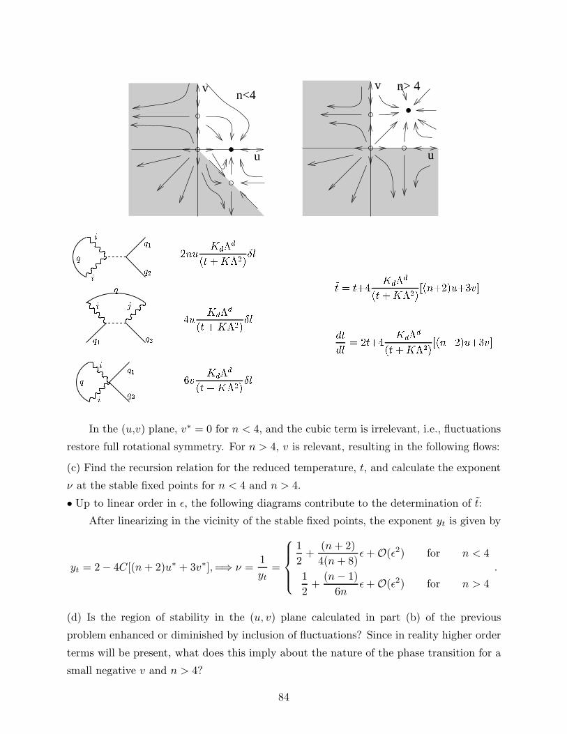
u
vn<4
u
v n> 4
q q2q1q1q2ii i jq
q1q ii q2~t = t+4 Kdd(t+K2)[(n+2)u+3v]dtdl = 2t+4 Kdd(t+K2) [(n+2)u+3v]
2nu Kdd(t+K2)l4u Kdd(t+K2)l6v Kdd(t +K2)l
In the (u,v) plane, v∗ = 0 for n < 4, and the cubic term is irrelevant, i.e., fluctuations
restore full rotational symmetry. For n > 4, v is relevant, resulting in the following flows:
(c) Find the recursion relation for the reduced temperature, t, and calculate the exponent
ν at the stable fixed points for n < 4 and n > 4.
• Up to linear order in ǫ, the following diagrams contribute to the determination of t:
After linearizing in the vicinity of the stable fixed points, the exponent yt is given by
yt = 2 − 4C[(n+ 2)u∗ + 3v∗],=⇒ ν =1
yt=
1
2+
(n+ 2)
4(n+ 8)ǫ+ O(ǫ2) for n < 4
1
2+
(n− 1)
6nǫ+ O(ǫ2) for n > 4
.
(d) Is the region of stability in the (u, v) plane calculated in part (b) of the previous
problem enhanced or diminished by inclusion of fluctuations? Since in reality higher order
terms will be present, what does this imply about the nature of the phase transition for a
small negative v and n > 4?
84

• All fixed points are located within the allowed region calculated in 1b). However, not
all flows starting in classically stable regions are attracted to stable fixed point. If the RG
flows take a point outside the region of stability, then fluctuations decrease the region of
stability. The domains of attraction of the fixed points for n < 4 and n > 4 are indicated
in the following figures: u+ v = 0u+ vn = 0
u vdomain of attractionunphysicaln > 4Flows which are not originally located within these domains of attraction flow into
the unphysical regions. The coupling constants u and v become more negative. This is
the signal of a fluctuation induced first order phase transition, by what is known as the
Coleman–Weinberg mechanism. Fluctuations are responsible for the change of order of the
transition in the regions of the (u,v) plane outside the domain of attraction of the stable
fixed points.
(e) Draw schematic phase diagrams in the (t, v) plane (u > 0) for n > 4 and n < 4,
identifying the ordered phases. Are there Goldstone modes in any of these phases close to
the phase transition?
• From the recursion relation obtained in 2c) for the parameter t, we obtain the following
non-trivial t∗
t∗ = −1
2[(n+ 2)u∗ + 3v∗] ∝ −ǫ
Therefore, the phase diagrams in the (t,v) plane is schematically represented as
As mentioned above, only when n < 4 fluctuations restore the full rotational symme-
try. The parameter v is renormalized to zero, and there are Goldstone modes at the (u,v)
plane, but only near the second order phase transition, where Kξ−2t = tv/(u+ v) → 0. In
the ordered phases, the renormalized value of v is finite, albeit small, indicating that there
are no Goldstone modes.
85

tvisotropic order
rst order boundarycubic axis orderdisordered phase
second order boundaryn < 4 t
vrst order boundarysecond order boundarydisordered phasediagonal order
cubic axis order n > 4********
5. Exponents: Two critical exponents at second order are,
ν =1
2+
(n+ 2)
4(n+ 8)ǫ+
(n+ 2)(n2 + 23n+ 60)
8(n+ 8)3ǫ2 ,
η =(n+ 2)
2(n+ 8)2ǫ2 .
Use scaling relations to obtain ǫ–expansions for two or more of the remaining exponents
α, β, γ, δ and ∆. Make a table of the results obtained by setting ǫ = 1, 2 for n = 1, 2
and 3; and compare to the best estimates of these exponents that you can find by other
sources (series, experiments, etc.).
********
6. Anisotropic criticality: A number of materials, such as liquid crystals, are anisotropic
and behave differently along distinct directions, which shall be denoted parallel and per-
pendicular, respectively. Let us assume that the d spatial dimensions are grouped into n
parallel directions x‖, and d− n perpendicular directions x⊥. Consider a one–component
field m(x‖,x⊥) subject to a Landau–Ginzburg Hamiltonian, βH = βH0 + U , with
βH0 =
∫
dnx‖dd−nx⊥
[
K
2(∇‖m)2 +
L
2(∇2
⊥m)2 +t
2m2 − hm
]
,
and U = u
∫
dnx‖dd−nx⊥ m4 .
86

(Note that βH depends on the first gradient in the x‖ directions, and on the second
gradient in the x⊥ directions.)
(a) Write βH0 in terms of the Fourier transforms m(q‖,q⊥).
• In terms of the Fourier modes m(q) =∫
ddxeiq·xm(x),
βH0 =
∫
dnq‖dd−nq⊥(2π)d
(
Kq2‖ + Lq4⊥ + t
2
)
|m(q)|2 − hm(q = 0).
(b) Construct a renormalization group transformation for βH0, by rescaling coordinates
such that q′‖ = b q‖ and q′
⊥ = c q⊥ and the field as m′(q′) = m(q)/z. Note that parallel
and perpendicular directions are scaled differently. Write down the recursion relations for
K, L, t, and h in terms of b, c, and z. (The exact shape of the Brillouin zone is immaterial
at this stage, and you do not need to evaluate the integral that contributes an additive
constant.)
• The unperturbed Hamiltonian describes a set of independent modes labelled by a wave-
vector q. We can integrate out the modes that correspond to short distance fluctuations,
and then rescale the parameters as suggested above to get
(βH0)′ = δf0
b +∫ dnq′
‖dd−nq′
⊥(2π)d
b−nc−(d−n)
(
Kb−2q′2‖ + Lc−4q′4⊥ + t
2
)
z2|m′(q′)|2 − zhm′(q′ = 0).
The renormalized bare Hamiltonian has the same form as βH0, with the renormalized
parameters
K ′ = b−(n+2)c−(d−n)z2K
L′ = b−nc−(d−n+4)z2L
t′ = b−nc−(d−n)z2t
h′ = zh
.
(c) Choose c(b) and z(b) such that K ′ = K and L′ = L. At the resulting fixed point
calculate the eigenvalues yt and yh for the rescalings of t and h.
• The requirements of K ′ = K and L′ = L lead to z2 = bn+2cd−n and z2 = bncd−n+4,
respectively. Consistency of these equations requires
c = b1/2, and z = b1+d+n
4 .
87

Inserting these results for c and z in the recursion relations for t and h, we find
t′ = b−n− d−n2 +2+ d+n
2 t = b2t
h′ = zh = b1+d+n
4 h, =⇒
yt = 2
hh = 1 +d+ n
4
.
(d) Write the relationship between the (singular parts of) free energies f(t, h) and f ′(t′, h′)
in the original and rescaled problems. Hence write the unperturbed free energy in the
homogeneous form f(t, h) = t2−αgf (h/t∆), and identify the exponents α and ∆.
• The RG transformation preserves the partition function Z, and the free energy density is
f ∼ lnZ/V . Under the rescaling transformation the volume changes to V ′ = b−nc−(d−n)V ,
and hence
f(t, h) = b−n− d−n2 f(t′, h′) = b−
d+n2 f
(
b2t, b1+d+n
4 h)
.
We can now rescale to a point at which b2t ∼ 1, at which point
f(t, h) = td+n
4 g
(
h
t12+ d+n
8
)
,
corresponding to
α = 2 − d+ n
4, and ∆ =
1
2+d+ n
8.
(e) How does the unperturbed zero–field susceptibility χ(t, h = 0), diverge as t→ 0?
• Taking two derivatives of the above free energy with respect to h, we obtain
χ ∼ ∂2f
∂h2∼ t
d+n4
(
t12+ d+n
8
)2
gχ
(
h
t12+ d+n
8
)
∼ t−1 (for h = 0) .
The zero-field susceptibility diverges with an exponent γ = 1 at t = 0. (The same result
can also be obtained by examining the two point correlation function.)
In the remainder of this problem set h = 0, and treat U as a perturbation.
(f) In the unperturbed Hamiltonian calculate the expectation value 〈m(q)m(q′)〉0, and the
corresponding susceptibility χ0(q) = 〈|mq|2〉0, where q stands for (q‖,q⊥).
• By examining the variance of the unperturbed Gaussian weight, we observe that
〈m(q)m(q′)〉0 = (2π)dδd(q + q′)χ0(q), with χ0(q) =1
t+Kq2‖ + Lq4⊥.
88

(g) Write the perturbation U , in terms of the normal modes m(q).
• After writing each of the four factors of m(x) in U in terms of m(q), and integrating
over all x, we obtain
U = u
∫
dq1dq2dq3m(q1)m(q2)m(q3)m(−q1 − q2 − q3),
where dq ≡ dnq‖dd−nq⊥/(2π)d.
(h) Using RG, or any other method, find the upper critical dimension du, for validity of
the Gaussian exponents.
• Under the rescaling steps outlined in the earlier parts of the problem, the coefficient of
the quartic perturbation changes to lowest order as
u′ = u(bc)−3z4 = ub−3nb−32 (d−n)b4+(d+n) ≡ ubyu , with yu = 4 − d+ n
2.
The upper critical dimension is identified as the point at which yu = 0, and thus
du = 8 − n.
(i) Write down the expansion for 〈m(q)m(q′)〉, to first order in U , and reduce the correction
term to a product of two point expectation values.
• Averages in perturbation theory are calculated as 〈O〉 = 〈O〉0−(〈OU〉0 − 〈O〉0〈U〉0)+· · ·.Using the expression for U in terms of Fourier modes, we find
〈m(q)m(q′)〉 =〈m(q)m(q′)〉0
− u
∫
dq1dq2dq3〈m(q)m(q′)m(q1)m(q2)m(q3)m(−q1 − q2 − q3)〉c0 +O(u2),
where the superscript ‘c’ in the first order correction stands for the cumulant. Using
Wick’s theorem the average of the six factors of m can be reduced to 12 equivalent pairwise
contractions, such that
〈m(q)m(q′)〉 =〈m(q)m(q′)〉0
−12u
∫
dq1dq2dq3〈m(q)m(q1)〉0〈m(q′)m(q2)〉0〈m(q3)m(−q1 − q2 − q3)〉0 +O(u2).
(j) Write down the expression for χ(q), in first order perturbation theory, and identify the
transition point tc at order of u. (Do not evaluate any integrals explicitly.)
89

• The two point expectation value has the form 〈m(q)m(q′)〉 = (2π)dδd(q + q′)χ(q), with
χ(q) =1
t+Kq2‖ + Lq4⊥− 12u
(t+Kq2‖ + Lq4⊥)2
∫
dk1
t+Kk2‖ + Lk4
⊥+O(u2)
=
[
t+Kq2‖ + Lq4⊥ + 12u
∫
dk1
t+Kk2‖ + Lk4
⊥+O(u2)
]−1
.
The inverse susceptibility χ(q = 0) should diverge at the critical point, t = tc, which is
thus identified as
tc = −12u
∫
dnk‖dd−nk⊥(2π)d
1
Kk2‖ + Lk4
⊥+O(u2).
********
7. Long–range interactions between spins can be described by adding a term∫
ddx
∫
ddyJ(|x− y|)~m(x) · ~m(y),
to the usual Landau–Ginzburg Hamiltonian.
(a) Show that for J(r) ∝ 1/rd+σ, the Hamiltonian can be written as
βH =
∫
ddq
(2π)d
t+K2q2 +Kσq
σ + · · ·2
~m(q) · ~m(−q)
+u
∫
ddq1ddq2d
dq3
(2π)3d~m(q1) · ~m(q2) ~m(q3) · ~m(−q1 − q2 − q3) .
• After changing variables to R = (x+y)/2, r = (x−y)/2, and writing the coarse-grained
spin as a sum of Fourier modes, the long-range interaction term becomes
∫
ddxddy~m(x) · ~m(y)
|x− y|d+σ=
∫
ddRddr1
rd+σ
∫ Λ ddq1ddq2
(2π)2d~m(q1) · ~m(q2)e
iq1·(R+r)eiq2·(R−r)
=
∫ Λ ddq
(2π)d~m(q) · ~m(−q)
∫
ddr1
|r|d+σe2iq·r = I
∫ Λ ddq
(2π)dqσ ~m(q) · ~m(−q).
The final expression is obtained by a rescaling of r = x/|q|, and I =∫
ddxe2ix1/|x|d+σ is
independent of q = |q|. Including the ever-present short-range parts, we can write the full
Hamiltonian as
βH =
∫
ddq
(2π)d
t+K2q2 +Kσq
σ + . . .
2~m(q) · ~m(−q)
+u
∫
ddq1ddq2d
dq3
(2π)3d~m(q1) · ~m(q2) ~m(q3) · ~m(−q1 − q2 − q3)
.
90

(b) For u = 0, construct the recursion relations for (t,K2, Kσ) and show that Kσ is
irrelevant for σ > 2. What is the fixed Hamiltonian in this case?
• For u = 0, the Gaussian integral over the outer-most shell will give us an additive
constant. Subsequent length q′ = bq, and spin m′ = m/z, rescalings lead to the following
recursion relations
t′ = b−dz2t
K ′2 = b−d−2z2K2
K ′σ = b−d−σz2Kσ
.
If σ > 2, the fixed point (t∗, K∗2 , K
∗σ) = (0, 0, Kσ) (obtained by choosing K ′
σ = Kσ) has no
basin of attraction, as
t′ = bσt
K ′2 = bσ−2K2
indicate two relevant directions; consequently, this fixed point does not describe the usual
critical point of the system. On the other hand, the fixed point (t∗, K∗2 , K
∗σ) = (0, K2, 0),
for which z2 = bd+2, leads to
t′ = b2t
K ′σ = b2−σKσ
,
i.e., it has one relevant and one irrelevant direction, and is therefore, the fixed point con-
trolling standard critical behavior of the system. In conclusion, if σ > 2, Kσ is irrelevant,
and the fixed Hamiltonian in this case is
βH∗ =K2
2
∫
ddq
(2π)dq2 ~m(q) · ~m(−q).
(c) For σ < 2 and u = 0, show that the spin rescaling factor must be chosen such that
K ′σ = Kσ, in which case K2 is irrelevant. What is the fixed Hamiltonian now?
• Conversely, for σ < 2, Kσ is the only relevant parameter at the fixed point (t∗, K∗2 , K
∗σ) =
(0, 0, Kσ), which is the one controlling the critical behavior in this case. At this point, the
spin scaling factor z, is chosen such that z2 = bd+σ, and the fixed Hamiltonian is
βH∗ =Kσ
2
∫
ddq
(2π)dqσ ~m(q) · ~m(−q).
(d) For σ < 2, calculate the generalized Gaussian exponents ν, η, and γ from the recursion
relations. Show that u is irrelevant, and hence the Gaussian results are valid, for d > 2σ.
91

• The divergence of the correlation length ξ, is controlled by the exponent ν = 1/yt. Since
ξ′ = ξot′ −ν = b−ytνξ, and ξ′ = ξ/b, the exponent ν is then
ν = 1/σ.
For σ < 2, the Gaussian correlation function in Fourier space is
χ(q) = (t+Kσqσ)−1,
and consequently,
χ = limq→0
χ(q) = t−1, with γ = 1.
In addition, at the critical point
χ(q) ∼ 1
q2−η, so η = 2 − σ.
If u 6= 0, at first order it will be renormalized to
u′ = b−3dz4u = b2σ−du,
indicating that u is irrelevant and the Gaussian results are valid provided that d > 2σ.
(e) For σ < 2, use a perturbation expansion in u to construct the recursion relations for
(t,Kσ, u) as in the text.
• Let us obtain the recursion relations for (t,Kσ, u). As shown in the text, the first order
diagrams and are zero; and contributes an additive constant. q
q2q1q1q2q u 2n Z =b ddq(2)d 1(t+Kq) = 2nu Kdd(t+K)l
u 4 Z =b ddq(2)d 1(t+Kq) = 4u Kdd(t+K)l92

The above two diagrams contribute to the coarse-grained parameter t. Their respective
contributions are obtained after considering b = eδl, and expanding the exponential to
linear order in the infinitesimal δl. The coarse-grained parameter t is then
t = t+ 2(2n+ 4)uKdΛ
d
t+KσΛσδl + O(u2).
At this order, the other parameters in the coarse grained Hamiltonian remain unchanged
(u = u, K2 = K2).
Taking into account the results of section 1.(b)-(c), after the usual steps 2 and 3
of the RG transformation, we obtain the following differential recursion relations for the
infinitesimal rescaling factor b ∼ 1 + δl:
t′ = bσ t
K ′2 = bσ−2K2
u′ = b2σ−du
, =⇒
dt
dl= σt+ 4u
(n+ 2)KdΛdδl
t+KσΛσ+ O(u2)
dK2
dl= (σ − 2)K2 + O(u2)
du
dl= (2σ − d)u+ O(u2)
.
For σ < 2 and d > 2σ, the Gaussian fixed point, which is the only solution of these equa-
tions, has only one relevant direction, describing correctly the phase transition. However,
if d < 2σ, there are two relevant directions, and we have to calculate the recursion relations
at the next order to find other non-trivial fixed points.
At second order in u, there are several new interactions proportional to m2, m4, m2q2,
which will appear in the coarse grained Hamiltonian. But of all these, we are essentially
interested in the second order diagrams which contribute to the renormalization of ~m4. As
shown in the text, these are:qq1 + q2 qq q4 00 q4q1 + q2 qqq1 + q2 q
q1q2q1q2q2q1
q3q3q4q3 u22 2 2 2nZ =b ddq(2)d 1(t+Kq)(t+Kjq1 + q2 qj) = 4nu2 Kdd(t+K)2 lu22 2 2 4 2Z =b ddq(2)d 1(t+Kq)(t+Kjq1 + q2 qj) = 16u2 Kdd(t+K)2 lu22 4 4 2Z =b ddq(2)d 1(t+Kq)(t+Kjq1 + q2 qj) = 16u2 Kdd(t+K)2 l
93

so that the new coarse grained parameters are
t = t+ 4u(n+ 2)KdΛ
d
t+KσΛσδl − u2Ct
K2 = K2 − u2CK2
Kσ = Kσ
u = u− 4u2 (n+ 8)KdΛd
(t+KσΛσ)2δl
.
Let us introduce the parameter ǫ = 2σ − d. After rescaling and renormalizing, we obtain
the following recursion relations:
dt
dl=σt+ 4u
(n+ 2)KdΛd
t+KσΛσ− u2Ct
du
dl=ǫu− 4u2 (n+ 8)KdΛ
d
(t+KσΛσ)2
.
(f) For d < 2σ, calculate the critical exponents ν and η to first order in ǫ = d− 2σ.
[See M.E. Fisher, S.-K. Ma and B.G. Nickel, Phys. Rev. Lett. 29, 917 (1972).]
• From the recursion relations, we can now obtain the non-trivial fixed point (t∗, u∗), which
satisfies dt/dl = du/dl = 0, as
u∗ =K2
σΛǫ
4(n+ 8)Kdǫ ≈ K2
σ
4(n+ 8)Kd=2σǫ
t∗ = −KσΛσ(n+ 2)
σ(n+ 8)ǫ
,
where, up to linear order in ǫ, we have set t = 0 in the denominators of both dt/dl and
du/dl, and performed other similar simplifications.
Linearizing the recursion relations in the vicinity of the non-trivial fixed point gives
d
dl
(
δt
δu
)
=
σ − (n+ 2)
(n+ 8)ǫ . . .
O(ǫ2) − ǫ
(
δt
δu
)
.
Hence the eigenvalues can be read directly from the diagonal elements of the matrix. The
first one is positive and controls the critical behavior, whereas the second is negative and
consequently irrelevant for d < 2σ.
94

The new exponent ν is then
ν =1
yt=
(
σ − (n+ 2)
(n+ 8)ǫ
)−1
=1
σ+
(n+ 2)
(n+ 8)σ2ǫ+ O(ǫ2),
and the exponent η remains the same as before, η = 2 − σ + O(ǫ2), since the parameter
Kσ has not been renormalized at linear order in ǫ. In fact, it can be shown that the RG
procedure only generates analytic corrections, and hence the coefficient of the non-analytic
term Kσ is unrenormalized to all orders, resulting in η = 2 − σ, exactly.
(g) What is the critical behavior if J(r) ∝ exp(−r/a)? Explain!
• A short-range interaction term of the form J(r) ∝ exp(−r/a) will modify the actual
value of the critical temperature Tc, and other non-universal quantities, but it will not
change the value of the critical exponents, since its Fourier transform is analytic:
∫
ddxddy~m(x) · ~m(y)e−|x−y|
a =
∫ Λ ddq
(2π)d~m(q) · ~m(−q)
∫
ddr e−ra e2iq·r
=
∫ Λ ddq
(2π)dC(q)~m(q) · ~m(−q),
where
C(q) = 2πad
∫ ∞
0
dxxd−1e−xJo(aqx) = ad∞∑
n=0
cn(qa)2n.
********
95

Solutions to problems from chapter 6- Lattice Systems
1. Cumulant method: Apply the Niemeijer–van Leeuwen first order cumulant expansion
to the Ising model on a square lattice with −βH = K∑
<ij> σiσj , by following these steps:
(a) For an RG with b = 2, divide the bonds into intra–cell components βH0; and inter–cell
components U .
• The N sites of the square lattice are partitioned into N/4 cells as indicated in the
figure below (the intra-cell and inter-cell bonds are represented by solid and dashed lines
respectively).
intra-cell bonds
inter-cell bonds
boundary ofnew unit blocks
The renormalized Hamiltonian βH′[σ′α] is calculated from
βH′ [σ′α] = − lnZ0 [σ′
α] + 〈U〉0 −1
2
(
⟨
U2⟩
0− 〈U〉20
)
+ O(
U3)
,
where 〈〉0 indicates expectation values calculated with the weight exp(−βH0) at fixed [σ′α].
(b) For each cell α, define a renormalized spin σ′α = sign(σ1
α + σ2α + σ3
α + σ4α). This choice
becomes ambiguous for configurations such that∑4
i=1 σiα = 0. Distribute the weight of
these configurations equally between σ′α = +1 and −1 (i.e. put a factor of 1/2 in addition
to the Boltzmann weight). Make a table for all possible configurations of a cell, the internal
probability exp(−βH0), and the weights contributing to σ′α = ±1.
96

+
+ +
+
+ +
+ +
+
+
+- -
-
-
-
Weighte4K
Weight4 1
4 1 12 2e4K 12
0 = 1
+ + +
+- -
-
-
- -
- -
+ -
- -
Weighte4K
Weight4 1
4 1 12 2e4K 12
0 = 1
• The possible intracell configurations compatible with a renormalized spin σ′α = ±1, and
their corresponding contributions to the intra-cell probability exp(−βH0), are given below,
resulting in
Z0 [σ′α] =
∏
α
(
e4K + 6 + e−4K)
=(
e4K + 6 + e−4K)N/4
.
(c) Express 〈U〉0 in terms of the cell spins σ′α; and hence obtain the recursion relation
K ′(K).
• The first cumulant of the interaction term is
−〈U〉0 = K∑
〈α,β〉〈σα2σβ1 + σα3σβ4〉0 = 2K
∑
〈α,β〉〈σα2〉0 〈σβ1〉0,
α β
1 12
34
2
34
97

where, for σ′α = 1,
〈σαi〉0 =e4K + (3 − 1) + 0 + 0
(e4K + 6 + e−4K)=
e4K + 2
(e4K + 6 + e−4K).
Clearly, for σ′α = −1 we obtain the same result with a global negative sign, and thus
〈σαi〉0 = σ′α
e4K + 2
(e4K + 6 + e−4K).
As a result,
−βH′ [σ′α] =
N
4ln(
e4K + 6 + e−4K)
+ 2K
(
e4K + 2
e4K + 6 + e−4K
)2∑
〈α,β〉σ′
ασ′β ,
corresponding to the recursion relation K ′(K),
K ′ = 2K
(
e4K + 2
e4K + 6 + e−4K
)2
.
(d) Find the fixed point K∗, and the thermal eigenvalue yt.
• To find the fixed point with K ′ = K = K∗, we introduce the variable x = e4K∗
. Hence,
we have to solve the equation
x+ 2
x+ 6 + x−1=
1√2, or
(√2 − 1
)
x2 −(
6 − 2√
2)
x− 1 = 0,
whose only meaningful solution is x ≃ 7.96, resulting in K∗ ≃ 0.52.
To obtain the thermal eigenvalue, let us linearize the recursion relation around this
non-trivial fixed point,
∂K ′
∂K
∣
∣
∣
∣
K∗
= byt , ⇒ 2yt = 1 + 8K∗[
e4K∗
e4K∗ + 2− e4K∗ − e−4K∗
e4K∗ + 6 + e−4K∗
]
, ⇒ yt ≃ 1.006.
(e) In the presence of a small magnetic field h∑
i σi , find the recursion relation for h; and
calculate the magnetic eigenvalue yh at the fixed point.
• In the presence of a small magnetic field, we will have an extra contribution to the
Hamiltonian
h∑
α,i
〈σα,i〉0 = 4he4K + 2
(e4K + 6 + e−4K)
∑
α
σ′α .
98

Therefore,
h′ = 4he4K + 2
(e4K + 6 + e−4K).
(f) Compare K∗, yt, and yh to their exact values.
• The cumulant method gives a value of K∗ = 0.52, while the critical point of the Ising
model on a square lattice is located at Kc ≈ 0.44. The exact values of yt and yh for the two
dimensional Ising model are respectively 1 and 1.875, while the cumulant method yields
yt ≈ 1.006 and yh ≈ 1.5. As in the case of a triangular lattice, yh is lower than the exact
result. Nevertheless, the thermal exponent yt is fortuitously close to its exact value.
********
2. Migdal–Kadanoff method: Consider Potts spins si = (1, 2, · · · , q), on sites i of a
hypercubic lattice, interacting with their nearest neighbors via a Hamiltonian
−βH = K∑
<ij>
δsi,sj.
(a) In d = 1 find the exact recursion relations by a b = 2 renormalization/decimation
process. Indentify all fixed points and note their stability.
• In d = 1, if we average over the q possible values of s1, we obtainq∑
s1=1
eK(δσ1s1+δs1σ2
) =
q − 1 + e2K if σ1 = σ2
q − 2 + 2eK if σ1 6= σ2
= eg′+K′δσ1σ2 ,
from which we arrive at the exact recursion relations:
eK′
=q − 1 + e2K
q − 2 + 2eK, eg′
= q − 2 + 2eK .
To find the fixed points we set K ′ = K = K∗. As in the previous problem, let us
introduce the variable x = eK∗
. Hence, we have to solve the equation
x =q − 1 + x2
q − 2 + 2x, or x2 + (q − 2)x− (q − 1) = 0,
whose only meaningful solution is x = 1, resulting in K∗ = 0. To check its stability, we
consider K ≪ 1, so that
K ′ ≃ ln
(
q + 2K + 2K2
q + 2K +K2
)
≃ K2
q≪ K,
which indicates that this fixed point is stable.
In addition, K∗ → ∞ is also a fixed point. If we consider K ≫ 1,
eK′ ≃ 1
2eK , =⇒ K ′ = K − ln 2 < K,
which implies that this fixed point is unstable.
**99

(b) Write down the recursion relation K ′(K) in d–dimensions for b = 2, using the Migdal–
Kadanoff bond moving scheme.
• In the Migdal-Kadanoff approximation, moving bonds strengthens the remaining bonds
by a factor 2d−1. Therefore, in the decimated lattice we have
eK′
=q − 1 + e2×2d−1K
q − 2 + 2e2d−1K.
(c) By considering the stability of the fixed points at zero and infinite coupling, prove the
existence of a non–trivial fixed point at finite K∗ for d > 1.
• In the vicinity of the fixed point K∗ = 0, i.e. for K ≪ 1,
K ′ ≃ 22d−2K2
q≪ K,
and consequently, this point is again stable. However, for K∗ → ∞, we have
eK′ ≃ 1
2exp
[(
2d − 2d−1)
K]
, =⇒ K ′ = 2d−1K − ln 2 ≫ K,
which implies that this fixed point is now stable provided that d > 1.
• As a result, there must be a finite K∗ fixed point, which separates the flows to the other
fixed points.
***(d) For d = 2, obtain K∗ and yt, for q = 3, 1, and 0.
• Let us now discuss a few particular cases in d = 2. For instance, if we consider q = 3,
the non-trivial fixed point is a solution of the equation
x =2 + x4
1 + 2x2, or x4 − 2x3 − x+ 2 = (x− 2)(x3 − 1) = 0,
which clearly yields a non-trivial fixed point at K∗ = ln 2 ≃ 0.69. The thermal exponent
for this point
∂K ′
∂K
∣
∣
∣
∣
K∗
= 2yt = 4
[
e4K∗
e4K∗ + 2− e2K∗
1 + 2e2K∗
]
=16
9, =⇒ yt ≃ 0.83,
which can be compared to the exact values, K∗ = 1.005, and yt = 1.2.
100

By analytic continuation for q → 1, we obtain
eK′
=e4K
−1 + 2e2K.
The non-trivial fixed point is a solution of the equation
x =x4
−1 + 2x2, or (x3 − 2x2 + 1) = (x− 1)(x2 − x− 1) = 0,
whose only non-trivial solution is x = (1 +√
5)/2 = 1.62, resulting in K∗ = 0.48. The
thermal exponent for this point
∂K ′
∂K
∣
∣
∣
∣
K∗
= 2yt = 4[
1 − e−K∗]
, =⇒ yt ≃ 0.61.
As discussed in the next problem set, the Potts model for q → 1 can be mapped onto the
problem of bond percolation, which despite being a purely geometrical phenomenon, shows
many features completely analogous to those of a continuous thermal phase transition.
And finally for q → 0, relevant to lattice animals (see PS#9), we obtain
eK′
=−1 + e4K
−2 + 2e2K,
for which we have to solve the equation
x =−1 + x4
−2 + 2x2, or x4 − 2x3 + 2x− 1 = (x− 1)3(x+ 1) = 0,
whose only finite solution is the trivial one, x = 1. For q → 0, if K ≪ 1, we obtain
K ′ ≃ K +K2
2> K,
indicating that this fixed point is now unstable. Note that the first correction only indicates
marginal stability (yt = 0). Nevertheless, for K∗ → ∞, we have
eK′ ≃ 1
2exp[2K], =⇒ K ′ = 2K − ln 2 ≫ K,
which implies that this fixed point is stable.
* *101

********
3. The Potts model: The transfer matrix procedure can be extended to Potts model,
where the spin si on each site takes q values si = (1, 2, · · · , q); and the Hamiltonian is
−βH = K∑N
i=1 δsi,si+1+KδsN ,s1
.
(a) Write down the transfer matrix and diagonalize it. Note that you do not have to solve
a qth order secular equation as it is easy to guess the eigenvectors from the symmetry of
the matrix.
• The partition function is
Z =∑
si< s1|T |s2 >< s2|T |s3 > · · · < sN−1|T |sN >< sN |T |s1 >= tr(TN ),
where < si|T |sj >= exp(
Kδsi,sj
)
is a q× q transfer matrix. The diagonal elements of the
matrix are eK , while the off-diagonal elements are unity. The eigenvectors of the matrix
are easily found by inspection. There is one eigenvectors with all elements equal; the
corresponding eigenvalue is λ1 = eK +q−1. There are also (q−1) eigenvectors orthogonal
to the first, i.e. the sum of whose elements is zero. This corresponding eigenvalues are
degenerate and equal to eK − 1. Thus
Z =∑
α
λNα =
(
eK + q − 1)N
+ (q − 1)(
eK − 1)N
.
(b) Calculate the free energy per site.
• Since the largest eigenvalue dominates for N ≫ 1,
lnZ
N= ln
(
eK + q − 1)
.
(c) Give the expression for the correlation length ξ (you don’t need to provide a detailed
derivation), and discuss its behavior as T = 1/K → 0.
• Correlations decay as the ratio of the eigenvalues to the power of the separation. Hence
the correlation length is
ξ =
[
ln
(
λ1
λ2
)]−1
=
[
ln
(
eK + q − 1
eK − 1
)]−1
.
102

In the limit of K → ∞, expanding the above result gives
ξ ≃ eK
q=
1
qexp
(
1
T
)
.
********
4. The spin–1 model: Consider a linear chain where the spin si at each site takes on
three values si = −1, 0, +1. The spins interact via a Hamiltonian
−βH =∑
i
Ksisi+1.
(a) Write down the transfer matrix 〈s|T |s′〉 = eKss′
explicitly.
• The explicit form of the 3x3 transfer matrix is
T =
eK 1 e−K
1 1 1e−K 1 eK
.
(b) Use symmetry properties to find the largest eigenvalue of T and hence obtain the
expression for the free energy per site (lnZ/N).
• Because of the symmetry of T , we guess an eigenvector of the form v1 =
1r1
. For an
eigenvalue λ, we then obtain the pair of equations
(
eK + e−K)
+ r = λ
2 + r = rλ, =⇒ r =
2
λ− 1= λ− 2 coshK.
This leads to the quadratic equation
λ2 − λ (1 + 2 coshK) − 2 (1 − coshK) = 0,
which has solutions
2λ± = 1 + 2 coshK ±√
1 + 4 coshK + 4 cosh2K + 8 − 8 coshK.
The partition function is related to the largest eigenvalue in the limit of large N , and hence
lnZ
N= lnλ+ = ln
[
1 + 2 coshK +√
1 + 4 coshK + 4 cosh2K + 8 − 8 coshK]
− ln 2.
103

(c) Obtain the expression for the correlation length ξ, and note its behavior as K → ∞.
• The second largest eigenvalue corresponds to the eigenvector v2 =
10−1
, and is equal
to
λ2 = eK − e−K = 2 sinhK.
The ratio of eigenvalues is related to the correlation length by
ξ =1
ln(λ1/λ2)= ln−1
[
1 + 2 coshK +√
1 + 4 coshK + 4 cosh2K + 8 − 8 coshK
4 sinhK
]
.
In the limit of large K,
λ1 ≃ eK(
1 + 4e−2K + · · ·)
, and λ2 ≃ eK(
1 − 2e−2K + · · ·)
,
such that the correlation length diverges as
limK→∞
ξ(K) ≃ e2K
5.
(d) If we try to perform a renormalization group by decimation on the above chain we find
that additional interactions are generated. Write down the simplest generalization of βHwhose parameter space is closed under such RG.
• The only symmetry present in the Hamiltonian is inversion, si → −si, and the
most general spin-1 Hamiltonian consistent with this symmetry is
B(s, s′) = g +Kss′ +µ
2
(
s2 + s′2)
+ ∆(ss′)2.
********
ectionClock model: Each site of the lattice is occupied by a q-valued spin si ≡1, 2, · · · , q, with an underlying translational symmetry modulus q, i.e. the system is in-
variant under si → (si + n)modq. The most general Hamiltonian subject to this symmetry
with nearest–neighbor interactions is
βHC = −∑
<i,j>
J(|si − sj|modq),
104

where J(n) is any function, e.g. J(n) = J cos(2πn/q). Potts models are a special case of
Clock models with full permutation symmetry, and Ising model is obtained in the limit of
q = 2.
(e) For a closed linear chain of N clock spins subject to the above Hamiltonian show that
the partition function Z = tr [exp(−βH)] can be written as
Z = tr [〈s1|T |s2〉〈s2|T |s3〉 · · · 〈sN |T |s1〉] ;
where T ≡ 〈si|T |sj〉 = exp [J(si − sj)] is a q × q transfer matrix.
• This is a simple generalization of the previous examples, and again the partition function
for N sites with period boundary conditions is Z = trTN , with the q × q matrix whose
elements are T ≡ 〈si|T |sj〉 = exp [J(si − sj)].
(f) Write down the transfer matrix explicitly and diagonalize it. Note that you do not
have to solve a qth order secular equation; because of the translational symmetry, the
eigenvalues are easily obtained by discrete Fourier transformation as
λ(k) =
q∑
n=1
exp
[
J(n) +2πink
q
]
.
• Because of the symmetry T ≡ 〈si|T |sj〉 = T (|s−s′|modq), we anticipate that eigenvectors
of the matrix have the simple form
vk =1√q
1ωk
ω2k
...ω(q−1)k
, where ω = e2πi/q is a qth root of unity.
It can then be explicitly verified that Tvk = λkvk, with
λk =
q∑
n=1
exp
[
J(n) +2πink
q
]
.
(g) Show that Z =∑q
k=1 λ(k)N ≈ λ(0)N for N → ∞. Write down the expression for the
free energy per site βf = − lnZ/N .
105

• For periodic boundary conditions
Z = trTN = λN0 + λN
1 + · · · = λN0
[
1 +
q−1∑
k=1
(
λk
λ0
)N]
.
For N → ∞, since λ0 is the largest eigenvalue, we obtain
βf = − lnZ
N= − lnλ0 = − ln
[
q−1∑
k=0
eJ(k)
]
.
(h) Show that the correlation function can be calculated from
⟨
δsi,si+ℓ
⟩
=1
Z
q∑
α=1
tr[
ΠαTℓΠαT
N−ℓ]
,
where Πα is a projection matrix. Hence show that⟨
δsi,si+ℓ
⟩
c∼ [λ(1)/λ(0)]ℓ. (You do not
have to explicitly calculate the constant of proportionality.)
• Consider the matrix Πα that has zero elements everywhere, except for a 1 for its (α, α)
element. Then⟨
δsi,si+ℓ
⟩
=1
Z
q∑
α=1
tr[
ΠαTℓΠαT
N−ℓ]
.
Evaluating the trace in the basis of (Fourier) eigenvectors gives
⟨
δsi,si+ℓ
⟩
=1
Z
q∑
α=1
∑
k,k′
< k′|Πα|k > λℓk < k|Πα|k′ > λN−ℓ
k′ .
The main contributions to the sum come from the the two largest eigenvalues, λ0 and λ1;
hence
⟨
δsi,si+ℓ
⟩
=1
λN0
q∑
α=1
[
λN0
1
q2+ λN−ℓ
0 λℓ1
(ωω∗)α
q2
]
=1
q
[
1 +
(
λ1
λ0
)ℓ]
≃ 1
qe−ℓ/ξ .
(Note that if the second eigenvalue is degenerate, there will also be a degeneracy factor.)
The correlation length is given as
ξ = ln−1
(
λ1
λ0
)
.
********
106

5. XY model: Consider two component unit spins ~si = (cos θi, sin θi) in one dimension,
with the nearest neighbor interactions described by −βH = K∑N
i=1 ~si · ~si+1.
(a) Write down the transfer matrix 〈θ|T |θ′〉, and show that it can be diagonalized with
eigenvectors fm(θ) ∝ eimθ for integer m.
• In the basis of the angles θi,
〈θ|T |θ′〉 = exp [K cos (θ − θ′)] .
The above transfer ‘matrix’ is diagonalized in the Fourier basis with 〈θ|m〉 = eimθ (not
normalized), as it is easily checked that
〈θ|T |θ′〉 〈θ′|m〉 =
∫ 2π
0
dθ′
2πeK cos(θ−θ′)+imθ′
= eimθ
∫ 2π
0
dφ
2πeK cos(φ)+imφ = λm〈θ|m〉,
with
λm =
∫ 2π
0
dφ
2πeK cos(φ)+imφ.
(b) Calulate the free energy per site, and comment on the behavior of the heat capacity
as T ∝ K−1 → 0.
• For large K the eigenvalues can be approximated by the saddle point method as
λm ≃ eK
2π
∫ ∞
−∞e−Kθ2/2+imθ =
eK
√2πK
e−m2
2K .
They are ordered with λ0 being the largest, and thus
lnZ
N≃ lnλ0 ≈ K − 1
2ln(2πK) + · · · .
The dimensionless parameter K can be related to a bond energy J by K = βJ , where
β = 1/(kBT ). Thus the energy of the chain in the limit of low temperatures is given by
E = −∂ lnZ
∂β= J
∂ lnZ
∂K= −NJ
(
1 − 1
2K+ ·)
= −NJ +NkBT
2+ · · · .
The first term is just the energy of the perfectly ordered chain. The second is the energy of
excitations into the harmonic modes. Since there areN such quadratic modes, the potential
energy of excitations is N × (kBT )/2. Note that since quantum effects are ignored, there
is no quenching of the oscillator energies, and a finite heat capacity of NkB/2 at zero
temperature.
107

(c) Find the correlation length ξ, and note its behavior as K → ∞.
• As usual, the correlation length is related to the ratio of the two largest eigenvalues as
ξ = − ln−1
(
λ1
λ0
)
≈(K→∞) 2K ∝ 1
T.
Note that the divergence of the correlation length as T → 0 is very different for cases where
there is a gap in the excitation energy (above the ground state), and when there is none.
********
6. One dimensional gas: The transfer matrix method can also be applied to a one
dimensional gas of particles with short-range interactions, as described in this problem.
(a) Show that for a potential with a hard core that screens the interactions from further
neighbors, the Hamiltonian for N particles can be written as
H =
N∑
i=1
p2i
2m+
N∑
i=2
V(xi − xi−1).
The (indistinguishable) particles are labeled with coordinates xi such that
0 ≤ x1 ≤ x2 ≤ · · · ≤ xN ≤ L,
where L is the length of the box confining the particles.
• Each particle i interacts only with adjacent particles i− 1 and i+ 1, as the hard cores
from these nearest neighbors screen the interactions with any other particle. Thus we
need only consider nearest neighbor interactions, and, included the kinetic energies, the
Hamiltonian is given by
H =
N∑
i=1
p2i
2m+
N∑
i=2
V(xi − xi−1), for 0 ≤ x1 ≤ x2 ≤ · · ·xN ≤ L.
(b) Write the expression for the partition function Z(T,N, L). Change variables to δ1 =
x1, δ2 = x2 − x1, · · · , δN = xN − xN−1, and carefully indicate the allowed ranges of
integration and the constraints.
108

• The partition function is
Z(T,N, L) =1
hN
∫ L
0
dx1
∫ L
x1
dx2 · · ·∫ L
xN−1
dxN exp
[
−βN∑
i=2
V(xi − xi−1)
]
·∫ ∞
−∞dp1 · · ·
∫ ∞
−∞dpN exp
[
−β∑
i=1
Np2
i
2m
]
=1
λN
∫ L
0
dx1
∫ L
x1
dx2 · · ·∫ L
xN−1
dxN exp
[
−βN∑
i=2
V(xi − xi−1)
]
,
where λ = h/√
2πmkBT . (Note that there is no N ! factor, as the ordering of the particles
is specified.) Introducing a new set of variables
δ1 = x1, δ2 = x2 − x1, · · · δn = xN − xN−1,
or equivalently
x1 = δ1, x2 = δ1 + δ2, · · · xN =
N∑
i=1
δi,
the integration becomes
Z(T,N, L) =1
λN
∫ L
0
dδ1
∫ L−δ1
0
dδ2
∫ L−(δ1+δ2)
0
dδ3 · · ·∫ L−
∑
N
i=1δi
0
dδNe−β∑N
i=2V(δi).
This integration can also be expressed as
Z(T,N, L) =1
λN
[∫
dδ1dδ2 · · ·dδN]′
exp
[
−βN∑
i=2
V(δi)
]
,
with the constraint
0 ≤N∑
i=1
δi ≤ L.
This constraint can be put into the equation explicitly with the use of the step function
Θ(x) =
0 for x < 0
1 for x ≥ 0,
as
Z(T,N, L) =1
λN
∫ ∞
0
dδ1
∫ ∞
0
dδ2 · · ·∫ ∞
0
dδN exp
[
−βN∑
i=2
V(δi)
]
Θ
(
L−N∑
i=1
δi
)
.
109

(c) Consider the Gibbs partition function obtained from the Laplace transformation
Z(T,N, P ) =
∫ ∞
0
dL exp(−βPL)Z(T,N, L),
and by extremizing the integrand find the standard formula for P in the canonical ensemble.
• The Gibbs partition function is
Z(T,N, P ) =
∫ ∞
0
dL exp(−βPL)Z(T,N, L).
The saddle point is obtained by extremizing the integrand with respect to L,
∂
∂Lexp(−βPL)Z(T,N, L)
∣
∣
∣
∣
T,N
= 0,
which implies that
βP =∂
∂LlnZ(T,N, L)
∣
∣
∣
∣
T,N
, =⇒ P = kBT∂ lnZ
∂L
∣
∣
∣
∣
T,N
.
From thermodynamics, for a one–dimensional gas we have
dF = −SdT − PdL, =⇒ P = − ∂F
∂L
∣
∣
∣
∣
T,N
.
Further noting that
F = −kBT lnZ,
again results in
Pcanonical = kBT∂ lnZ
∂L
∣
∣
∣
∣
T,N
.
(d) Change variables from L to δN+1 = L−∑Ni=1 δi, and find the expression for Z(T,N, P )
as a product over one-dimensional integrals over each δi.
• The expression for the partition function given above is
Z(T,N, L) =1
λN
∫ ∞
0
dδ1
∫ ∞
0
dδ2 · · ·∫ ∞
0
dδN exp
[
−βN∑
i=2
V(δi)
]
Θ
(
L−N∑
i=1
δi
)
.
110

The Laplace transform of this equation is
Z(T,N, P ) =1
λN
∫ ∞
0
dL exp(−βPL)
∫ ∞
0
dδ1
∫ ∞
0
dδ2 · · ·∫ ∞
0
dδN
· exp
[
−βN∑
i=2
V(δi)
]
Θ
(
L−N∑
i=1
δi
)
=1
λNβP
∫ ∞
0
dδ1
∫ ∞
0
dδ2 · · ·∫ ∞
0
dδN exp
[
−βN∑
i=2
V(δi)
]
exp
[
−βP(
N∑
i=1
δ1
)]
=1
λN (βP )2
∫ ∞
0
dδ2 · · ·∫ ∞
0
dδN exp
−N∑
i=2
[βV(δi) + βPδi]
.
Since the integrals for different δ′is are equivalent, we obtain
Z(T,N, P ) =1
λN (βP )2
∫ ∞
0
dδ exp [−β (V(δ) + Pδ)]
N−1
.
This expression can also be obtained directly, without use of the step function as follows.
Z(T,N, P ) =1
λN
∫ L
0
dδ1
∫ L−δ1
0
dδ2
∫ L−(δ1+δ2)
0
dδ3 · · ·∫ L−
∑
N
i=1δi
0
dδN
·∫ ∞
0
dL exp
[
−βPL− β
(
N∑
i=2
V(δ)
)]
=1
λN
∫ L
0
dδ1
∫ L−δ1
0
dδ2 · · ·∫ L−
∑N
i=1δi
0
dδN
∫ ∞
−∑N
i=1δi
d
(
L−N∑
i=1
δi
)
· exp
−βP[
N∑
i=1
δi +
(
L−N∑
i=1
δi
)]
− β
(
N∑
i=2
V(δi)
)
.
Change variables to δN+1 ≡ L −∑Ni=1 δi, and note that each of the δ′s indicates the
distance between neighboring particles. The size of the gas L, has been extended to any
value, hence each δ can be varied independently from 0 to ∞. Thus the Gibbs partition
111

function is
Z(T,N, P ) =1
λN
∫ ∞
0
dδ1
∫ ∞
0
dδ2 · · ·∫ ∞
0
dδN
∫ ∞
0
dδN+1
· exp
[
−βP(
N+1∑
i=1
δi
)
− β
(
N∑
i=2
V(δi)
)]
=1
λN
(∫ ∞
0
dδ · exp [−βV(δ) − βPδ]
)N−1 ∫ ∞
0
dδ1 exp(−βPδ1)
·∫ ∞
0
dδN+1 exp(−βPδN+1)
=1
λN (βP )2
∫ ∞
0
dδ exp [−β (V(δ) + Pδ)]
N−1
.
(e) At a fixed pressure P , find expressions for the mean length L(T,N, P ), and the density
n = N/L(T,N, P ) (involving ratios of integrals which should be easy to interpret).
• The mean length is
L(T,N, P ) = −kBT∂
∂(βP )lnZ(T,N, P )
∣
∣
∣
∣
T,N
=2
βP+ (N − 1)
∫∞0dδ · δ · exp [−βV(δ) − βPδ]
∫∞0dδ · exp [−βV(δ) − βPδ]
,
and the density n is given by
n =N
L(T,N, P )= N
2kBT
P+ (N − 1)
∫∞0dδ · δ · exp [−β (V(δ) − Pδ)]
∫∞0dδ · exp [−β (V(δ) − Pδ)]
−1
.
Note that for an ideal gas V i.g.(δ) = 0, and
Li.g.(T,N, P ) =(N + 1)kBT
P,
leading to
n(p)i.g. =N
N + 1
P
kBT.
Since the expression for n(T, P ) in part (e) is continuous and non-singular for any
choice of potential, there is in fact no condensation transition for the one-dimensional
gas. By contrast, the approximate van der Waals equation (or the mean-field treatment)
incorrectly predicts such a transition.
112

(f) For a hard sphere gas, with minimum separation a between particles, calculate the
equation of state P (T, n).
• For a hard sphere gas
δi ≥ a, for i = 2, 3, · · · , N,the Gibbs partition function is
Z(T,N, P ) =1
λN (βP )2
[∫ ∞
a
dδ exp (−βV(δ) − βPδ)
]N−1
=1
λN (βP )2
[∫ ∞
a
dδ exp (−βPδ)]N−1
=1
λN
(
1
βP
)N+1
exp (−βPa)N−1.
From the partition function, we can calculate the mean length
L = −kBT∂ lnZ∂P
∣
∣
∣
∣
T,N
=(N + 1)kBT
P+ (N − 1)a,
which after rearrangement yields
βP =(N + 1)
L− (N − 1)a=
n+ 1/L
1 − (n− 1/L)a≈ (n+ 1/l)(1 + (n− 1/L)a+ (n− 1/L)2a2 + · · ·).
For N ≫ 1, n≫ 1/L, and
βP ≈ n(1 + na+ n2a2 + · · ·) = n+ an2 + a2n3 + · · · ,which gives the virial coefficients
Bℓ(T ) = aℓ−1.
The value of B3 = a2 agrees with the result obtained in an earlier problem. Also note
that the exact ‘excluded volume’ is (N − 1)a, as opposed to the estimate of Na/2 used in
deriving the van der Waals equation.
********
7. Potts chain (RG): Consider a one-dimensional array of N Potts spins si = 1, 2, · · · , q,subject to the Hamiltonian −βH = J
∑
i δsi,si+1.
(a) Using the transfer matrix method (or otherwise) calculate the partition function Z,
and the correlation length ξ.
•(b) Is the system critical at zero temperature for antiferromagnetic couplings J < 0?
•
113

(c) Construct a renormalization group (RG) treatment by eliminating every other spin.
Write down the recursion relations for the coupling J , and the additive constant g.
•
(d) Discuss the fixed points, and their stability.
•
(e) Write the expression for lnZ in terms of the additive constants of successive rescalings.
•(f) Show that the recursion relations are simplified when written in terms of t(J) ≡e−1/ξ(J).
•
114

(g) Use the result in (f) to express the series in (e) in terms of t. Show that the answer
can be reduced to that obtained in part (a), upon using the result
∞∑
n=0
1
2n+1ln
(
1 + t2n
1 − t2n
)
= − ln(1 − t).
•
(h) Repeat the RG calculation of part (c), when a small symmetry breaking term h∑
i δsi,1
is added to −βH. You will find that an additional coupling term K∑
i δsi,1δsi+1,1 is gen-
erated under RG. Calculate the recursion relations in the three parameter space (J,K, h).
115

•(i) Find the magnetic eigenvalues at the zero temperature fixed point where J → ∞, and
obtain the form of the correlation length close to zero temperature.
•********
8. Cluster RG: Consider Ising spins on a hexagonal lattice with nearest neighbor interac-
tions J .
(a) Group the sites into clusters of four in preparation for a position space renormalization
group with b = 2.
•(b) How can the majority rule be modified to define the renormalized spin of each cluster.
•
116

(c) For a scheme in which the central site is chosen as the tie–breaker, make a table of all
possible configurations of site–spins for a given value of the cluster–spin.
•(d) Focus on a pair of neighboring clusters. Indicate the contributions of intra–cluster and
inter–cluster bonds to the total energy.
•(e) Show that in zero magnetic field, the Boltzmann weights of parallel and anti-parallel
clusters are given by
R(+,+) = x8 + 2x6 + 7x4 + 14x2 + 17 + 14x−2 + 7x−4 + 2x−6,
and
R(+,−) = 9x4 + 16x2 + 13 + 16x−2 + 9x−4 + x−8,
117

where x = eJ .
• Summing over the contributions in the previous tables gives the answer quoted above.
(f) Find the expression for the resulting recursion relation J ′(J).
•
118

(g) Estimate the critical ferromagnetic coupling Jc, and the exponent ν obtained from this
RG scheme, and compare with the exact values.
• The non-trivial fixed point occurs at J∗ ≈ 1.05, while the exact value of the hexagonal
lattice critical coupling is Jc ≈ 0.66. The value of the eigenvalue yt and hence the exponent
ν = 1/yt is close to the exact value of 1.
(h) What are the values of the magnetic and thermal exponents (yh, yt) at the zero tem-
perature ferromagnetic fixed point?
•
(i) Is the above scheme also applicable for anti-ferromagnetic interactions? What symmetry
of the original problem is not respected by this transformation?
• The distinction between the two sublattices of the hexagonal lattice is not respected by
this RG scheme, and hence it does not reproduce the anti-ferromagnetic phase transition.
********
9. Transition probability matrix: Consider a system of two Ising spins with a coupling
K, which can thus be in one of four states.
(a) Explicitly write the 4 × 4 transition matrix corresponding to single spin flips for a
Metropolis algorithm. Verify that the equilibrium weights are indeed a left eigenvector of
this matrix.
(b) Repeat the above exercise if both single spin and double spin flips are allowed. The
two types of moves are chosen randomly with probabilities p and q = 1 − p.
********
119

Solutions to problems from chapter 7 - Series Expansions
1. Continuous spins: In the standard O(n) model, n component unit vectors are placed
on the sites of a lattice. The nearest neighbor spins are then connected by a bond J~si ·~sj.
In fact, if we are only interested in universal properties, any generalized interaction f(~si ·~sj)
leads to the same critical behavior. By analogy with the Ising model, a suitable choice is
exp [f(~si · ~sj)] = 1 + (nt)~si · ~sj ,
resulting in the so called loop model.
(a) Construct a high temperature expansion of the loop model (for the partition function
Z) in the parameter t, on a two-dimensional hexagonal (honeycomb) lattice.
• The partition function for the loop model has the form
Z =
∫
Dsi∏
〈ij〉[1 + (nt)si · sj ] ,
that we can expand in powers of the parameter t. If the total number of nearest neighbor
bonds on the lattice is NB, the above product generates 2NB possible terms. Each term
may be represented by a graph on the lattice, in which a bond joining spins i and j is
included if the factor si · sj appears in the term considered. Moreover, each included bond
carries a factor of nt. As in the Ising model, the integral over the variables si leaves only
graphs with an even number of bonds emanating from each site, because
∫
ds sα =
∫
ds sαsβsγ = · · · = 0.
In a honeycomb lattice, as plotted below, there are only 1, 2, or 3 bonds emerging
from each site. Thus the only contributing graphs are those with two bonds at each site,
which, as any bond can only appear once, are closed self-avoiding loops.
61
3
2
45
120

While the honeycomb lattice has the advantage of not allowing intersections of loops at a
site, the universal results are equally applicable to other lattices.
We shall rescale all integrals over spin by the n-dimensional solid angle, such that∫
ds = 1. Since sαsα = 1, it immediately follows that∫
ds sαsβ =δαβ
n,
resulting in∫
ds′ (sαs′α)(s′βs
′′β) =
1
nsαs
′′α.
A sequence of such integrals forces the components of the spins around any loop to be the
same, and there is a factor n when integrating over the last spin in the loop, for instance∫
Dsi (s1αs2α)(s2βs3β)(s3γs4γ)(s4δs5δ)(s5ηs6η)(s6νs1ν) =δαβδβγδγδδδηδηνδαν
n6=
n
n6.
Since each bond carrier a factor of nt, each loop finally contributes a factor n× tℓ, where
ℓ is the number of bonds in the loop. The partition function may then be written as
Z =∑
self−avoiding loops
nNℓtNb ,
where the sum runs over distinct disconnected or self-avoiding loops collections with a
bond fugacity t, and Nℓ, Nb are the number of loops, and the number of bonds in the
graph, respectively. Note that, as we are only interested in the critical behavior of the
model, any global analytic prefactor is unimportant.
(b) Show that the limit n→ 0 describes the configurations of a single self–avoiding polymer
on the lattice.
• While Z = 1, at exactly n = 0, one may obtain non-trivial information by considering
the limit n→ 0. The leading term (O(n1)) when n→ 0 picks out just those configurations
with a single self-avoiding loop, i.e. Nℓ = 1.
n
m
121

The correlation function can also be calculated graphically from
Gαβ(n−m) = 〈snαsmβ〉 =1
Z
∫
Dsisnαsmβ
∏
〈ij〉[1 + (nt)si · sj ] .
After disregarding any global prefactor, and taking the limit n → 0, the only surviving
graph consists of a single line going from n to m, and the index of all the spins along
the line is fixed to be the same. All other possible graphs disappear in the limit n → 0.
Therefore, we are left with a sum over self-avoiding walks that go from n to m, each
carrying a factor tℓ, where ℓ indicates the length of the walk. If we denote by Wℓ(R) the
number of self-avoiding walks of length ℓ whose end-to-end distance is R, we can write
that∑
ℓ
Wℓ(R)tℓ = limn→0
G(R).
As in the case of phantom random walks, we expect that for small t, small paths
dominate the behavior of the correlation function. As t increases, larger paths dominate
the sum, and, ultimately, we will find a singularity at a particular tc, at which arbitrarily
long paths become possible.
Although we presented the mapping of self-avoiding walks to the n → 0 limit of
the O(n) model for a honeycomb lattice, the critical behavior should be universal, and
therefore independent of this lattice choice. What is more, various scaling properties of
self-avoiding walks can be deduced from the O(n) model with n→ 0. Let us, for instance,
characterize the mean square end-to-end distance of a self-avoiding walk, defined as
⟨
R2⟩
=1
Wℓ
∑
R
R2Wℓ(R),
where Wℓ =∑
RWℓ(R) is the total number of self-avoiding walks of length ℓ.
The singular part of the correlation function decays with separation R as G ∝|R|−(d−2+η), up to the correlation length ξ, which diverges as ξ ∝ (tc − t)−ν . Hence,
∑
R
R2G(R) ∝ ξd+2−(d−2+η) = (tc − t)−ν(4−η) = (tc − t)−γ−2ν .
We noted above that G(t, R) is the generating function of Wℓ(R), in the sense that∑
ℓWℓ(R)tℓ = G(t, R). Similarly∑
ℓWℓtℓ is the generating function of Wℓ, and is re-
lated to the susceptibility χ, by
∑
ℓ
Wℓtℓ =
∑
R
G(R) = χ ∝ (tc − t)−γ .
122

To obtain the singular behavior of Wℓ from its generating function, we perform a Taylor
expansion of (tc − t)−γ , as
∑
ℓ
Wℓtl = t−γ
c
(
1 − t
tc
)−γ
= t−γc
∑
ℓ
Γ(1 − γ)
Γ(1 + ℓ)Γ(1 − γ − ℓ)
(
t
tc
)ℓ
,
which results in
Wℓ =Γ(1 − γ)
Γ(1 + ℓ)Γ(1 − γ − ℓ)t−ℓ−γc .
After using that Γ(p)Γ(1− p) = π/ sin pπ, considering ℓ→ ∞, and the asymptotic expres-
sion of the gamma function, we obtain
Wℓ ∝Γ(γ + ℓ)
Γ(1 + ℓ)t−ℓc ∝ ℓγ−1t−ℓ
c ,
and, similarly one can estimate∑
RR2Wℓ(R) from
∑
RR2G(R), yielding
⟨
R2⟩
∝ ℓ2ν+γ−1t−ℓc
ℓγ−1t−ℓc
= ℓ2ν .
Setting n = 0 in the results of the ǫ-expansion for the O(n) model, for instance, gives the
exponent ν = 1/2 + ǫ/16 + O(ǫ2), characterizing the mean square end-to-end distance of
a self-avoiding polymer as a function of its length ℓ, rather than ν0 = 1/2 which describes
the scaling of phantom random walks. Because of self-avoidance, the (polymeric) walk is
swollen, giving a larger exponent ν. The results of the first order expansion for ǫ = 1, 2,
and 3, in d = 3, 2, and 1 are 0.56, 0.625, and 0.69, to be compared to 0.59, 3/4 (exact),
and 1 (exact).
********
2. Potts model I: Consider Potts spins si = (1, 2, · · · , q), interacting via the Hamiltonian
−βH = K∑
<ij> δsi,sj.
(a) To treat this problem graphically at high temperatures, the Boltzmann weight for each
bond is written as
exp(
Kδsi,sj
)
= C(K) [1 + T (K)g(si, sj)] ,
with g(s, s′) = qδs,s′ − 1. Find C(K) and T (K).
• To determine the two unknowns C(K) and T (K), we can use the expressions
eK = C [1 + T (q − 1)] if si = sj
1 = C [1 − T ] if si 6= sj
,
123

from which we obtain
T (K) =eK − 1
eK + q − 1, and C(K) =
eK + q − 1
q.
(b) Show that
q∑
s=1
g(s, s′) = 0 ,
q∑
s=1
g(s1, s)g(s, s2) = qg(s1, s2) , and
q∑
s,s′
g(s, s′)g(s′, s) = q2(q − 1).
• Moreover, it is easy to check that
q∑
s=1
g(s, s′) = q − 1 − (q − 1) = 0,
q∑
s=1
g(s1, s)g(s, s2) =
q∑
s=1
[
q2δs1sδs2s − q(δs1s + δs2s) + 1]
= q (qδs1s2− 1) = qg(s1, s2),
q∑
s,s′=1
g(s, s′)g(s, s′) =
q∑
s,s′=1
[
q2δss′δss′ − 2qδss′ + 1]
= q3 − 2q2 + q2 = q2(q − 1).
(c) Use the above results to calculate the free energy, and the correlation function
〈g(sm, sn)〉 for a one–dimensional chain.
• The factor T (K) will be our high temperature expansion parameter. Each bond con-
tributes a factor Tg(si, sj) and, since∑
s g(s, s′) = 0, there can not be only one bond per
any site. As in the Ising case considered in lectures, each bond can only be considered
once, and the only graphs that survive have no dangling bonds. As a result, for a one-
dimensional chain, with for instance open boundary conditions, it is impossible to draw
any acceptable graph, and we obtain
Z =∑
si
∏
〈ij〉C(K) [1 + T (K)g(si, sj)] = C(K)N−1qN = q
(
eK + q − 1)N−1
.
Ignoring the boundary effects, i.e., that there are N −1 bonds in the chain, the free energy
per site is obtained as
−βFN
= ln(
eK + q − 1)
.
124

With the same method, we can also calculate the correlation function 〈g(snsm)〉. To get a
nonzero contribution, we have to consider a graph that directly connects these two sites.
Assuming that n > m, this gives
〈g(snsm)〉 =C(K)N
Z
∑
sig(snsm)
∏
〈ij〉[1 + T (K)g(si, sj)]
=C(K)N
ZT (K)n−m
∑
sig(snsm)g(sm, sm+1) · · · g(sn−1, sn)
=C(K)N
ZT (K)n−mqn−m+1(q − 1)qN−(n−m)−1 = Tn−m(q − 1)
where we have used the relationships obtained in (b).
(d) Calculate the partition function on the square lattice to order of T 4. Also calculate
the first term in the low–temperature expansion of this problem.
• The first term in the high temperature series for a square lattice comes from a square of
4 bonds. There are a total of N such squares. Therefore,
Z =∑
si
∏
〈ij〉C(K) [1 + T (K)g(si, sj)] = C(K)2NqN
[
1 +NT (K)4(q − 1) + · · ·]
.
Note that any closed loop involving ℓ bonds without intersections contributes T ℓqℓ(q− 1).
On the other hand, at low temperatures, the energy is minimized by the spins all
being in one of the q possible states. The lowest energy excitation is a single spin in a
different state, resulting in an energy cost of K × 4 with a degeneracy factor N × (q − 1),
resulting in
Z = qe2NK[
1 +N(q − 1)e−4K + · · ·]
.
(e) By comparing the first terms in low- and high–temperature series, find a duality rule
for Potts models. Don’t worry about higher order graphs, they will work out! Assuming
a single transition temperature, find the value of Kc(q).
• Comparing these expansions, we find the following duality condition for the Potts model
e−K = T (K) =eK − 1
eK + q − 1.
This duality rule maps the low temperature expansion to a high temperature series, or vice
versa. It also maps pairs of points, K ⇔ K, since we can rewrite the above relationship
in a symmetric way(
eK − 1)(
eK − 1)
= q,
125

and consequently, if there is a single singular point Kc, it must be self-dual point,
Kc = Kc, =⇒ Kc = ln (√q + 1) .
(f) How do the higher order terms in the high–temperature series for the Potts model
differ from those of the Ising model? What is the fundamental difference that sets apart
the graphs for q = 2? (This is ultimately the reason why only the Ising model is solvable.)
• As mentioned in lectures, the Potts model with q = 2 can be mapped to the Ising model
by noticing that δss′ = (1 + ss′)/2. However, higher order terms in the high-temperature
series of the Potts model involve, in general, graphs with three or more bonds emanating
from each site. These configurations do not correspond to a random walk, not even a
constrained one as introduced in class for the 2d Ising model on a square lattice. The
quantity
q∑
s1=1
g(s1, s2)g(s1, s3)g(s1, s4) = q3δs2s3δs2s4
− q2(δs2s3+ δs2s4
+ δs3s4) + 2q,
is always zero when q = 2 (as can be easily checked for any possible state of the spins s2, s3
and s4), but is in general different from zero for q > 2. This is the fundamental difference
that ultimately sets apart the case q = 2. Note that the corresponding diagrams in the
low temperature expansion involve adjacent regions in 3 (or more) distinct states.
********
3. Potts model II: An alternative expansion is obtained by starting with
exp [Kδ(si, sj)] = 1 + v(K)δ(si, sj),
where v(K) = eK − 1. In this case, the sum over spins does not remove any graphs, and
all choices of distributing bonds at random on the lattice are acceptable.
(a) Including a magnetic field h∑
i δsi,1, show that the partition function takes the form
Z(q,K, h) =∑
all graphs
∏
clusters c in graph
[
vncb ×
(
q − 1 + ehncs
)]
,
where ncb and nc
s are the numbers of bonds and sites in cluster c. This is known as the
random cluster expansion.
126

• Including a symmetry breaking field along direction 1, the partition function
Z =∑
si
∏
〈ij〉[1 + v(K)δ(si, sj)]
∏
i
ehδsi,1 ,
can be expanded in powers of v(K) as follows. As usual, if there is a total number NB
of nearest neighbor bonds on the lattice, the product over bonds generates 2NB possible
terms. Each term may be represented by a graph on the lattice, in which a bond joining
sites i and j is included if the factor vδ(si, sj) appears in the term considered. Each
included bond carries a factor v(K), as well as a delta function enforcing the equality of
the spins on the sites which it connects. In general, these bonds form clusters of different
sizes and shapes, and within each cluster, the delta functions force the spins at each vertex
to be the same. The sum∑
si therefore gives a factor of (q−1)+ ehncs for each cluster c,
where ncs is the number of point in the cluster. The partition function may then be written
as
Z(q, v, h) =∑
all graphs
∏
clusters in graph
[
v(K)ncb
(
q − 1 + ehnsc
)]
,
where ncb is the number of bonds in cluster c, and the sum runs over all distinct cluster
collections. Note that an isolated site is also included in this definition of a cluster. While
the Potts model was originally defined for integer q, using this expansion, we can evaluate
Z for all values of q.
127

(b) Show that the limit q → 1 describes a percolation problem, in which bonds are randomly
distributed on the lattice with probability p = v/(v+1). What is the percolation threshold
on the square lattice?
• In the problem of bond percolation, bonds are independently distributed on the lattice,
with a probability p of being present. The weight for a given configuration of occupied
and absent bonds bonds is therefore
W (graph) = (1 − p)zN∏
clusters in graph
(
p
1 − p
)ncb
.
The prefactor of (1 − p)zN is merely the weight of the configuration with no bonds. The
above weights clearly become identical to those appearing in the random cluster expansion
of the Potts model for q = 1 (and h = 0). Clearly, we have to set p = v/(v + 1), and
neglect an overall factor of (1+v)N , which is analytic in v, and does not affect any singular
behavior. The partition function itself is trivial in this limit as Z(1, v, h) = (1 + v)zNehN .
On the other hand, we can obtain information on the number of clusters by considering
the limit of q → 1 from
∂ lnZ(q, v)
∂q
∣
∣
∣
∣
q=1
=∑
all graphs
[probablility of graph]∑
clusters in graph
e−hnsc .
Various properties of interest to percolation can then be calculated from the above
generating function. This mapping enables us to extract the scaling laws at the percola-
tion point, which is a continuous geometrical phase transition. The analog of the critical
temperature is played by the percolation threshold pc, which we can calculate using the
expression obtained in problem 2 as pc = 1/2 (after noting that v∗ = 1).
An alternative way of obtaining this threshold is to find a duality rule for the percola-
tion problem itself: One can similarly think of the problem in terms of empty bonds with
a corresponding probability q. As p plays the role of temperature, there is a mapping of
low p to high q or vice versa, and such that q = 1−p. The self-dual point is then obtained
by setting p∗ = 1 − p∗, resulting in p∗ = 1/2.
(c) Show that in the limit q → 0, only a single connected cluster contributes to leading
order. The enumeration of all such clusters is known as listing branched lattice animals.
128

• The partition function Z(q, v, h) goes to zero at q = 0, but again information about
geometrical lattice structure can be obtain by taking the limit q → 0 in an appropriate
fashion. In particular, if we set v = qax, then
Z(q, v = xqa, h = 0) =∑
all graphs
xNbqNc+aNb ,
where Nb and Nc are the total number of bonds and clusters. The leading dependence
on q as q → 0 comes from graphs with the lowest number of Nc + aNb, and depends on
the value of a. For 0 < a < 1, these are the spanning trees, which connect all sites of the
lattice (hence Nc = 1) and that enclose no loops (hence Nb = N − 1). Such spanning trees
have a power of xa(N−1)qaN−a+1, and all other graphs have higher powers of q. For a = 0
one can add bonds to the spanning cluster (creating loops) without changing the power,
as long as all sites remain connected in a single cluster. These have a relation to a problem
referred to as branched lattice animals.
********
4. Ising model in a field: Consider the partition function for the Ising model (σi = ±1)
on a square lattice, in a magnetic field h; i.e.
Z =∑
σiexp
K∑
<ij>
σiσj + h∑
i
σi
.
(a) Find the general behavior of the terms in a low–temperature expansion for Z.
• At low temperatures, almost all the spins are oriented in the same direction; low energy
excitations correspond to islands of flipped spins. The general behavior of the terms in a
low-temperature expansion of the partition function is then of the form
e−2KLe−2hA,
where L is the perimeter of the island, or the number of unsatisfied bonds, and A is the
area of the island, or the number of flipped spins.
- -+
+
+
+
+
+
+ -
+
+
+
L=4, A=1 L=6, A=2
129

(b) Think of a model whose high–temperature series reproduces the generic behavior found
in (a); and hence obtain the Hamiltonian, and interactions of the dual model.
• To reproduce terms that are proportional to the area, we may consider plaquette-like
interactions of the form
h∑
plaquettes
σ1σ2σ3σ4,
where σ is a spin variable defined on each bond of the lattice. Thus, we can define a (lattice
gauge) model whose Hamiltonian is given by
−βH = K∑
bonds
σ + h∑
plaquettes
σ1σ2σ3σ4,
and, as usual, rewrite
eKσ = cosh K(
1 + tanh K)
σ,
ehσ1σ2σ3σ4 = cosh h(
1 + tanh h)
σ1σ2σ3σ4.
The high temperature series of the partition function will be then of the form,
Z ∝∑
bonds
∑
plaquettes
(
tanh K)Nb
(
tanh h)Np
,
where Nb and Np, are the number of bonds and plaquettes involved in each term of the
expansion. Nevertheless, we will only have non-zero contributions when the bond variables
σ, appear an even number of times, either in a plaquette or as a bond. For example, the
lowest order contributions contain 1 plaquette (so that A = 1), and 4 extra bonds (L = 4),
or 2 plaquettes (A = 2), and 6 bonds (L = 6), etc.
L=4, A=1 L=6, A=2
σσσ σ
130

In general, we obtain terms of the form
(
tanh K)L (
tanh h)A
,
with L and A, the perimeter and the area of the graph considered. Hence, as in the Ising
model, we can write the duality relations
e−2K = tanh K, and e−2h = tanh h.
********
5. Potts duality: Consider Potts spins, si = (1, 2, · · · , q), placed on the sites of a square
lattice of N sites, interacting with their nearest-neighbors through a Hamiltonian
−βH = K∑
<ij>
δsi,sj.
(a) By comparing the first terms of high and low temperature series, or by any other
method, show that the partition function has the property
Z(K) = qe2NKΞ[
e−K]
= q−N[
eK + q − 1]2N
Ξ
[
eK − 1
eK + (q − 1)
]
,
for some function Ξ, and hence locate the critical point Kc(q).
• As discussed in problem 3 of this chapter, the low temperature series takes the form
Z = qe2NK[
1 +N(q − 1)e−4K + · · ·]
≡ qe2NKΞ[
e−K]
,
while at high temperatures
Z =
[
eK + q − 1
q
]2N
qN
[
1 +N(q − 1)
(
eK − 1
eK + q − 1
)4
+ · · ·]
≡ q−N[
eK + q − 1]2N
Ξ
[
eK − 1
eK + q − 1
]
.
Both of the above series for Ξ are in fact the same, leading to the duality condition
e−K =eK − 1
eK + q − 1,
131

and a critical (self-dual) point of
Kc = Kc, =⇒ Kc = ln (√q + 1) .
(b) Starting from the duality expression for Z(K), derive a similar relation for the internal
energy U(K) = 〈βH〉 = −∂ lnZ/∂ lnK. Use this to calculate the exact value of U at the
critical point.
• The duality relation for the partition function gives
lnZ(K) = ln q + 2NK + lnΞ[
e−K]
= −N ln q + 2N ln[
eK + q − 1]
+ ln Ξ
[
eK − 1
eK + q − 1
]
.
The internal energy U(K) is then obtained from
−U(K)
K=
∂
∂KlnZ(K) = 2N − e−K ln Ξ′ [e−K
]
= 2NeK
eK + q − 1+
qeK
(eK + q − 1)2 lnΞ′
[
eK − 1
eK + q − 1
]
.
ln Ξ′ is the derivative of lnΞ with respect to its argument, whose value is not known in
general. However, at the critical point Kc, the arguments of lnΞ′ from the high and low
temperature forms of the above expression are the same. Substituting eKc = 1 +√q, we
obtain
2N − ln Ξ′c
1 +√q
=2N√q
+ln Ξ′
c
1 +√q, =⇒ ln Ξ′
c =q − 1√qN,
and,
−U(Kc)
Kc= N
(
2 − q − 1√q + q
)
, =⇒ U(Kc) = NKc
√q + 1√q
.
********
6. Anisotropic random walks: Consider the ensemble of all random walks on a square
lattice starting at the origin (0,0). Each walk has a weight of t ℓxx × t
ℓyy , where ℓx and ℓy
are the number of steps taken along the x and y directions respectively.
(a) Calculate the total weight W (x, y), of all walks terminating at (x, y). Show that W is
well defined only for t = (tx + ty)/2 < tc = 1/4.
132

• Defining 〈0, 0|W (ℓ) |x, y〉 to be the weight of all walks of ℓ steps terminating at (x, y),
we can follow the steps in sec.VI.F of the lecture notes. In the anisotropic case, Eq.(VI.47)
(applied ℓ times) is trivially recast into
〈x, y|T ℓ |qx, qy〉 =∑
x′,y′
〈x, y|T ℓ |x′, y′〉 〈x′, y′| qx, qy〉
=(2tx cos qx + 2ty cos qy)ℓ 〈x, y| qx, qy〉 ,
where 〈x, y| qx, qy〉 = eiqxx+iqyy/√N . Since W (x, y) =
∑
ℓ 〈0, 0|W (ℓ) |x, y〉, its Fourier
transform is calculated as
W (qx, qy) =∑
ℓ
∑
x,y
〈0, 0|T ℓ |x, y〉 〈x, y| qx, qy〉
=∑
ℓ
(2tx cos qx + 2ty cos qy)ℓ=
1
1 − (2tx cos qx + 2ty cos qy).
Finally, Fourier transforming back gives
W (x, y) =
∫ π
−π
d2q
(2π)2W (qx, qy) e−iqxx−iqyy =
∫ π
−π
d2q
(2π)2
e−iqxx−iqyy
1 − (2tx cos qx + 2ty cos qy).
Note that the summation of the series is legitimate (for all q’s) only for 2tx + 2ty < 1, i.e.
for t = (tx + ty) /2 < tc = 1/4.
(b) What is the shape of a curve W (x, y) = constant, for large x and y, and close to the
transition?
• For x and y large, the main contributions to the above integral come from small q’s. To
second order in qx and qy, the denominator of the integrand reads
1 − 2 (tx + ty) + txq2x + tyq
2y .
Then, with q′i ≡√tiqi, we have
W (x, y) ≈∫ ∞
−∞
d2q′
(2π)2 √
txty
e−iq′·v
1 − 2 (tx + ty) + q′2 ,
where we have extended the limits of integration to infinity, and v =
(
x√tx, y√
ty
)
. As the
denominator is rotationally invariant, the integral depends only on the magnitude of the
vector v. In other words, W (x, y) is constant along ellipses
x2
tx+y2
ty= constant.
133

(c) How does the average number of steps, 〈ℓ〉 = 〈ℓx + ℓy〉, diverge as t approaches tc?
• The weight of all walks of length ℓ, irrespective of their end point location, is
∑
x,y
〈0, 0|W (ℓ) |x, y〉 = 〈0, 0|T ℓ |qx = 0, qy = 0〉 = (2tx + 2ty)ℓ= (4t )
ℓ.
Therefore,
〈ℓ〉 =
∑
ℓ ℓ (4t )ℓ
∑
ℓ (4t )ℓ
= 4t∂
∂ (4t )ln
[
∑
ℓ
(4t )ℓ
]
= 4t∂
∂ (4t )ln
1
1 − 4t=
4t
1 − 4t,
i.e.
〈ℓ〉 =t
tc − t,
diverges linearly close to the singular value of t.
********
7. Anisotropic Ising model: Consider the anisotropic Ising model on a square lattice
with a Hamiltonian
−βH =∑
x,y
(
Kxσx,yσx+1,y +Kyσx,yσx,y+1
)
;
i.e. with bonds of different strengths along the x and y directions.
(a) By following the method presented in the text, calculate the free energy for this model.
You do not have to write down every step of the derivation. Just sketch the steps that
need to be modified due to anisotropy; and calculate the final answer for lnZ/N .
• The Hamiltonian
−βH =∑
x,y
(Kxσx,yσx+1,y +Kyσx,yσx,y+1) ,
leads to
Z =∑
(2 coshKx coshKy)Ntℓxx t
ℓyy ,
where ti = tanhKi, and the sum runs over all closed graphs. By extension of the isotropic
case,
f =lnZ
N= ln (2 coshKx coshKy) +
∑
ℓx,ℓy
tℓxx t
ℓyy
ℓx + ℓy〈0|W ∗ (ℓx, ℓy) |0〉 ,
134

where
〈0|W ∗ (ℓx, ℓy) |0〉 =1
2
′∑
(−1)number of crossings
,
and the primed sum runs over all directed (ℓx, ℓy)-steps walks from (0, 0) to (0, 0) with
no U-turns. As in the isotropic case, this is evaluated by taking the trace of powers
of the 4N × 4N matrix described by Eq.(VI.66), which is block diagonalized by Fourier
transformation. However, unlike the isotropic case, in which each element is multiplied by
t, here they are multiplied by tx and ty, respectively, resulting in
f = ln (2 coshKx coshKy) +1
2
∫
d2q
(2π)2 tr ln
[
1 − T (q)∗],
where
tr ln[
1 − T (q)∗]
= ln det[
1 − T (q)∗]
= ln[(
1 + t2x) (
1 + t2y)
− 2tx(
1 − t2y)
cos qx − 2ty(
1 − t2x)
cos qy]
= ln
[
cosh 2Kx cosh 2Ky − sinh 2Kx cos qx − sinh 2Ky cos qycosh 2Kx cosh 2Ky
]
,
resulting in
f = ln 2 +1
2
∫
d2q
(2π)2 ln (cosh 2Kx cosh 2Ky − sinh 2Kx cos qx − sinh 2Ky cos qy) .
(b) Find the critical boundary in the (Kx, Ky) plane from the singularity of the free energy.
Show that it coincides with the condition Kx = Ky, where K indicates the standard dual
interaction to K.
• The argument of the logarithm is minimal at qx = qy = 0, and equal to
cosh 2Kx cosh 2Ky − sinh 2Kx − sinh 2Ky
=1
2
(
eKx√
cosh 2Ky − 1 − e−Kx√
cosh 2Ky + 1)2
.
Therefore, the critical line is given by
e2Kx =
√
cosh 2Ky + 1
cosh 2Ky − 1= cothKy.
Note that this condition can be rewritten as
sinh 2Kx =1
2(cothKy − tanhKy) =
1
sinh 2Ky,
135

i.e. the critical boundary can be described as Kx = Ky, where the dual interactions, K
and K, are related by sinh 2K sinh 2K = 1.
(c) Find the singular part of lnZ/N , and comment on how anisotropy affects critical
behavior in the exponent and amplitude ratios.
• The singular part of lnZ/N for the anisotropic case can be written as
fS =1
2
∫
d2q
(2π)2 ln
(
eKx√
cosh 2Ky − 1 − e−Kx√
cosh 2Ky + 1)2
+∑
i=x,y
q2i2
sinh 2Ki
.
In order to rewrite this expression in a form closer to that of the singular part of the free
energy in the isotropic case, let
qi =
√
2
sinh 2Kiq′i,
and
δt = eKx√
cosh 2Ky − 1 − e−Kx√
cosh 2Ky + 1
(δt goes linearly through zero as (Kx, Ky) follows a curve which intersects the critical
boundary). Then
fS =1
√
sinh 2Kx sinh 2Ky
∫
d2q′
(2π)2 ln
(
δt2 + q′2)
.
Thus, upon approaching the critical boundary (sinh 2Kx sinh 2Ky = 1), the singular part
of the anisotropic free energy coincides more and more precisely with the isotropic one,
and the exponents and amplitude ratios are unchanged by the anisotropy. (The amplitude
itself does vary along the critical line.)
********
8. Muller–Hartmann and Zittartz estimate of the interfacial energy of the d = 2 Ising
model on a square lattice.
(a) Consider an interface on the square lattice with periodic boundary conditions in one
direction. Ignoring islands and overhangs, the configurations can be labeled by heights hn
for 1 ≤ n ≤ L. Show that for an anisotropic Ising model of interactions (Kx, KY ), the
energy of an interface along the x-direction is
−βH = −2KyL− 2Kx
∑
n
|hn+1 − hn| .
136

1 2 N. . .
h1
hN
+ + + + + + + + + + + + + + +++ + + + + + + + + + + + + + +
+ + + + + + + + + + + + + + +
+ + + + + + + + + + + + + +
+
+
+
+
+
+
+
+
+ + +
+
+
+
+
+
+
+
- - - - - - - - --- - - - - - - - - - - - - - -
- - - - - - - - - - - - - -
- - - - -- - -
- - - -- -
--
• For each unsatisfied (+−) bond, the energy is increased by 2Ki from the ground state
energy, with i = x if the unsatisfied bond is vertical, and i = y if the latter is horizontal.
Ignoring islands and overhangs, the number of horizontal bond of the interface is L, while
the number of vertical bonds is∑
n |hn+1 − hn|, yielding
−βH = −2KyL− 2Kx
L∑
n=1
|hn+1 − hn| .
(b) Write down a column–to–column transfer matrix 〈h|T |h′〉, and diagonalize it.
• We can define
〈h|T |h′〉 ≡ exp (−2Ky − 2Kx |h′ − h|) ,
or, in matrix form,
T = e−2Ky
1 e−2Kx e−4Kx · · · e−HKx e−HKx e−2(H2 −1)Kx · · · e−2Kx
e−2Kx 1 e−2Kx · · · e−2(H2 −1)Kx e−2(H
2 +1)Kx e−HKx · · · e−4Kx
· · ·
whereH is the vertical size of the lattice. In theH → ∞ limit, T is easily diagonalized since
each line can be obtained from the previous line by a single column shift. The eigenvectors
of such matrices are composed by the complex roots of unity (this is equivalent to the
statement that a translationally invariant system is diagonal in Fourier modes). To the
eigenvector(
ei 2πk , ei 2π
k ·2, ei 2πk ·3, · · · , ei 2π
k ·(H+1))
,
137

is associated the eigenvalue
λk = e−2Ky
H+1∑
n=1
T1nei 2π
k ·(n−1).
Note that there are H + 1 eigenvectors, corresponding to k = 1, · · · , H + 1.
(c) Obtain the interface free energy using the result in (b), or by any other method.
• One way of obtaining the free energy is to evaluate the largest eigenvalue of T . Since all
elements of T are positive, the eigenvector (1, 1, · · · , 1) has the largest eigenvalue
λ1 = e−2Ky
H+1∑
n=1
T1n = e−2Ky
1 + 2
H/2∑
n=1
e−2Kxn
= e−2Ky
2
H/2∑
n=0
e−2Kxn − 1
= e−2Ky cothKx,
in the H → ∞ limit. Then, F = −LkBT lnλ1.
Alternatively, we can directly sum the partition function, as
Z = e−2KyL∑
hnexp
(
−2Kx
L∑
n=1
|hn+1 − hn|)
= e−2KyL
[
∑
d
exp (−2Kx |d|)]L
=
e−2Ky
2∑
d≥0
e−2Kxd − 1
L
=(
e−2Ky cothKx
)L,
yielding
F = −LkBT [ln (cothKx) − 2Ky] .
(d) Find the condition between Kx and Ky for which the interfacial free energy vanishes.
Does this correspond to the critical boundary of the original 2d Ising model as computed
in the previous problem?
• The interfacial free energy vanishes for
cothKx = e2Ky ,
which coincides with the condition found in problem 2. This illustrates that long wave-
length fluctuations, such as interfaces, are responsible for destroying order at criticality.
********
138

9. Anisotropic Landau theory: Consider an n–component magnetization field ~m(x) in
d–dimensions.
(a) Using the previous problems on anisotropy as a guide, generalize the standard Landau–
Ginzburg Hamiltonian to include the effects of spacial anisotropy.
• Requiring different coupling constants in the different spatial directions, along with
rotational invariance in spin space, leads to the following leading terms of the Hamiltonian,
−βH =
∫
ddx
[
t
2~m (x)
2+
d∑
i=1
Ki
2
∂ ~m
∂xi· ∂ ~m∂xi
+ u~m (x)4
]
.
(b) Are such anisotropies “relevant?”
• Clearly, the apparent anisotropy can be eliminated by the rescaling
x′i =
√
K
Kixi.
In terms of the primed space variables, the Hamiltonian is isotropic. In particular, the
universal features are identical in the anisotropic and isotropic cases, and the anisotropy
is thus “irrelevant” (provided all Ki are non-vanishing).
(c) In La2CuO4, the Cu atoms are arranged on the sites of a square lattice in planes, and
the planes are then stacked together. Each Cu atom carries a spin which we assume to
be classical, and can point along any direction in space. There is a very strong antifer-
romagnetic interaction in each plane. There is also a very weak inter-plane interaction
that prefers to align successive layers. Sketch the low–temperature magnetic phase, and
indicate to what universality class the order–disorder transition belongs.
• For classical spins, this combination of antiferromagnetic and ferromagnetic couplings is
equivalent to a purely ferromagnetic (anisotropic) system, since we can redefine (e.g. in
the partition function) all the spins on one of the two sublattices with an opposite sign.
Therefore, the critical behavior belongs to the d = 3, n = 3 universality class.
Nevertheless, there is a range of temperatures for which the in-plane correlation length
is large compared to the lattice spacing, while the inter-plane correlation length is of the
order of the lattice spacing. The behavior of the system is then well described by a d = 2,
n = 3 theory.
********
10. Energy by duality: Consider the Ising model (σi = ±1) on a square lattice with
−βH = K∑
<ij> σiσj .
139

(a) Starting from the duality expression for the free energy, derive a similar relation for
the internal energy U(K) = 〈H〉 = −∂ lnZ/∂ lnK.
• The low temperature partition function has the form
Z(K) = e2KN∑
islands
e−2KL,
whereas the high temperature expansion looks like
Z(K) =(
2 cosh2K)N ∑
loops
(tanhK)L.
What is more, we found that we can write a duality relation of the form
tanhK = e−2K , or sinh 2K sinh 2K = 1,
which we can use to rewrite the partition function as
Z(K) =(
2 cosh2K)N
e−2KNZ(K) = (sinh 2K)NZ(K),
yielding
−βF (K) = N ln(2 sinh 2K) − βF (K).
The internal energy U(K) is then obtained from
U(K) = −K ∂
∂KlnZ(K) = −NK 2 cosh 2K
sinh 2K−K
(
∂
∂KlnZ(K)
)
∂K
∂K.
After taking the logarithm of the relation sinh 2K sinh 2K = 1, and differentiating it, we
obtain∂K
∂K= −tanh 2K
tanh 2K,
and, as a result
U(K) = −2NK coth 2K − K
KU(K)
tanh 2K
tanh 2K
or, equivalently
U(K)tanh 2K
K+ U(K)
tanh 2K
K= −2N.
(b) Using (a), calculate the exact value of U at the critical point Kc.
140

• Using the last result, we can calculate the exact value of U at the critical point, K∗ =
K = K,
U(K∗) = − NK∗
tanh 2K∗ = −N√
2
2ln(
√2 + 1),
where we have used K∗ = ln(√
2 + 1)/2, and sinh 2K∗ = 1.
********
11. Clock model duality: Consider spins si = (1, 2, · · · , q) placed on the sites of a square
lattice, interacting via the clock model Hamiltonian
βHC = −∑
<i,j>
J (|(si − sj)modq|) ,
(a) Change from the N site variables to the 2N bond variables bij = si − sj. Show
that the difference in the number of variables can be accounted for by the constraint that
around each plaquette (elementary square) the sum of the four bond variables must be
zero modulus q.
• Around any closed loop, e.g. for the four bonds making up an elementary square,
Sp ≡∑
bpij =∑
(si − sj) = 0,
as any si appears once with a positive and once with a negative sign. We may insist that
all bond variables are positive, using bij = (si − sj)modq, in which case the above equality
is also valid modulus q.
(b) The constraints can be implemented by adding “delta–functions”
δ [Sp]modq =1
q
q∑
np=1
exp
[
2πinpSp
q
]
,
for each plaquette. Show that after summing over the bond variables, the partition function
can be written in terms of the dual variables, as
Z = q−N∑
np
∏
〈p,p′〉λ (np − np′) ≡
∑
npexp
∑
〈p,p′〉J (np − np′)
,
where λ(k) is the discrete Fourier transform of eJ(n).
141

• In terms of the constrained bond variables, the partition function is
Z =∑
bij
∏
p
δ [Sp]modq
∏
<ij>
eJ(bij) =∑
bij
∏
p
∑
np
1
qexp
[
2πinp
q
∑
bpij
]
∏
<ij>
eJ(bij).
Now we can do the sum over each bond variable bij independently. Note, however, that a
given bij appears twice in the constraints appropriate to its adjacent plaquettes, say p and
p′, and thus contributes
∑
bij
exp
[
2πibijq
(np − np′) + J (bij)
]
≡ λ(np − np′) ≡ eJ(np−np′).
The difference in the exponent is again meaningful modulus q, and thus
Z = q−N∑
np
∏
〈p,p′〉eJ(np−np′) =
∑
npexp
∑
〈p,p′〉J (np − np′)
.
(c) Calculate the dual interaction parameter of a Potts model, and hence locate the critical
point Jc(q).
• For the Potts model, the discrete Fourier transform has only two values. If np = np′ ,
then
λ(np = np′) = eJ + q − 1,
and otherwise
λ(np 6= np′) = eJ − 1,
since the sum of all roots of unity (excluding one itself) is minus one. The ratio of these
two cases gives the dual Potts interaction as
eJ =eJ + q − 1
eJ − 1.
Assuming that there is only one critical point (which is correct), it has to be at the self-dual
point jc(q) = Jc(q). This leads to a quadratic equation for x = eJc(q),
x2 − 2x− (q − 1) = 0, =⇒ x = 1 +√
q − 1, =⇒ Jc(q) = ln[
1 +√
q − 1]
.
142

(d) Construct the dual of the anisotropic Potts model, with
−βH =∑
x,y
(
Jxδsx,y,sx+1,y+ Jyδsx,y,sx,y+1
)
;
i.e. with bonds of different strengths along the x and y directions. Find the line of self–dual
interactions in the plane (Jx, Jy).
• The dual of the anisotropic square lattice is another anisotropic square lattice with
Jx = lneJy + q − 1
eJy − 1, and Jy = ln
eJx + q − 1
eJx − 1.
It is easy to check that the ˜J = J , and hence Jy = Jx is a line that maps onto itself under
duality. It turns out that this is also the critical line of the anisotropic Potts model on the
square lattice.
********
12. Triangular/hexagonal lattice Ising model: For any planar network of bonds, one
can define a geometrical dual by connecting the centers of neighboring plaquettes. Each
bond of the dual lattice crosses a bond of the original lattice, allowing for a local mapping.
Clearly, the dual of a triangular lattice is a hexagonal (or honeycomb) lattice, and vice
versa.
(a) Consider the Ising models on a hexagonal lattice with nearest neighbor interaction
strength Kh. Note that the hexagonal lattice is bipartite, i.e. can be separated into two
sublattices. In the partition function, do a partial sum over all spins in one sublattice.
Show that the remaining spins form a triangular lattice with nearest neighbor interaction
Kt(Kh). (This is called the star–triangle transformation.)
•
143

(b) Show that the dual of a triangular Ising model is a hexagonal Ising model with the
usual duality relation K(K).
•
144

(c) By combining the previous results, obtain the critical couplingsK∗t andK∗
h of triangular
and hexagonal lattices.
•
********
13. Triangular/hexagonal lattice Potts model: The steps of the previous problem can be
repeated for a general Potts model.
(a) Consider Potts spins (si = 1, 2, · · · , q) on a hexagonal lattice with nearest neighbor
interaction Khδsi,sj. Perform the star-triangle decimation to show that the remaining
spins form a triangular lattice with nearest neighbor interaction Kt(Kh), and a three spin
interaction L(Kh). Why is L absent in the Ising model?
•(b) What is the dual of the Potts model on the triangular lattice?
•
145

(c) Clearly, the model is not self–dual due to the additional interaction. Nonetheless,
obtain the critical value such that Kt(Kc) = Kc. Then check that L(Kc) = 0, i.e. while
the model in general is not self–dual, it is self–dual right at criticality, leading to the exact
value of Kc(q)!
•
146

********
14. Cubic lattice: The geometric concept of duality can be extended to general dimensions
d. However, the dual of a geometric element of dimension D is an entity of dimension d−D.
For example, the dual of a bond (D = 1) in d = 3 is a plaquette (D = 2), as demonstrated
in this problem.
(a) Consider a clock model on a cubic lattice of N points. Change to the 3N bond variables
bij = si − sj . (Note that one must make a convention about the positive directions on the
three axes.) Show that there are now 2N constraints associated with the plaquettes of this
lattice.
147

(b) Implement the constraints through discrete delta-functions by associating an auxiliary
variable np with each plaquette. It is useful to imagine np as defined on a bond of the dual
lattice, perpendicular to the plaquette p.
(c) By summing over the bond variables in Z, obtain the dual Hamiltonian
˜βH =∑
p
J (np12 − np
23 + np34 − np
41) ,
where the sum is over all plaquettes p of the dual lattice, with
npij
indicating the four
bonds around plaquette p.
(d) Note that ˜βH is left invariant if all the six bonds going out of any site are simultaneously
increased by the same integer. Thus unlike the original model which only had a global
translation symmetry, the dual model has a local, i.e. gauge symmetry.
(e) Consider a Potts gauge theory defined on the plaquettes of a four dimensional hyper-
cubic lattice. Find its critical coupling Jc(q).
148

********
Percolation
Fluids do not pass through a solid with a small concentration of holes. However,
beyond a threshold concentration, the holes overlap, and the fluid can percolate through
149

a connected channel in the material. Percolation is a classical geometric phase transition,
and has been used as a model of many breakdown or failure processes. The loss of rigidity
in an elastic network, conductivity in resistor nets, magnetization in diluted magnets are
but a few examples.
In simple models of percolation, elements of a lattice (sites or bonds) are independently
occupied with a probability p. A cluster is defined as a connected (by neighboring bonds)
set of these occupied elements. At small p, only small clusters exist, and the probability
that two sites, separated by a distance r, are connected to each other decays as exp (−r/ξ).The correlation length ξ(p) grows with increasing p, diverging at the percolation threshold
pc as ξ(p) ∼ |pc − p|−ν . An infinite cluster first appears at this threshold, and percolates
through the (infinite) system for all p > pc. The analog of the order parameter is the
probability P (p) that a site belongs to this infinite cluster. On approaching pc from above,
it vanishes as P (p) ∼ |pc − p|β. While the value of pc depends on the details of the model,
the exponents β and ν are universal, varying only with the spatial dimension d.
In the following problems we shall focus on bond percolation, i.e. p denotes the
probability that a bond on the lattice is occupied.
15. Cayley trees: Consider a hierarchical lattice in which each site at one level is connected
to z sites at the level below. Thus the n-th level of the tree has zn sites.
(a) For z = 2, obtain a recursion relation for the probability Pn(p) that the top site of a
tree of n levels is connected to some site at the bottom level.
•
150

(b) Find the limiting behavior of P (p) for infinitely many levels, and give the exponent β
for this tree.
•
(c) In a mean-field approximation, P (p) for a lattice of coordination number z is calculated
self-consistently, in a manner similar to the above. Give the mean-field estimates for pc
and the exponent β.
•
151

(d) The one-dimensional chain corresponds to z = 1. Find the probability that end-points
of an open chain of N + 1 sites are connected, and hence deduce the correlation length ξ.
•********
16. Duality has a very natural interpretation in percolation: If a bond is occupied, its dual
is empty, and vice versa. Thus the occupation probability for dual bonds is p = 1− p ≡ q.
Since, by construction, the original and dual elements do not intersect, one or the other
percolates through the system.
(a) The dual of a chain in which N bonds are connected in series, has N bonds connected
in parallel. What is the corresponding (non-) percolation probability?
• Consider N bonds forming a circle (1d chain with periodic boundary conditions). The
dual system has one point inside the circle and one point outside. While on the original
chain neighboring points are connected in series with probability p, on the dual lattice,
the inside and outside points are connected by N dual bonds in parallel with probability
q = 1 − p, i.e. a connected path on the original chain blocks a possible dual path. The
probability that the original chain is connected is pN . The probability that the two dual
points are not connected is also pN .
(b) The bond percolation problem on a square lattice is self-dual. What is its threshold
pc?
• The dual to the square lattice is another square lattice whose sites are the centers of the
squares of the original lattice. If a bond is not connected on the original lattice, a path
exists between the centers of neighboring squares. Thus p = 1−p = q. The self-dual point,
which is the bond percolation threshold occurs at pc = 1/2.
(c) Bond percolation in three dimensions is dual to plaquette percolation. Is it possible to
percolate while maintaining solid integrity in d = 3?
• Yes, there is an intermediate range of values between pc and pc in which both bonds and
plaquettes percolate.
152

(d) The triangular and hexagonal lattices are dual to each other. Combined with the star–
triangle transformation that also maps the two lattices, this leads to exact values of pc for
these lattices. However, this calculation is not trivial, and it is best to follow the steps for
calculations of the critical couplings of q-state Potts models in an earlier problem.
********
17. Position–space renormalization group (PSRG): In the Migdal–Kadanoff approxima-
tion, a decimation is performed after bonds are moved to connect the remaining sites in a
one-dimensional geometry. For a PSRG rescaling factor b on a d–dimensional hypercubic
lattice, the retained sites are connected by bd−1 strands in parallel, each strand having b
bonds in series. This scheme is naturally exact for d = 1, and becomes progressively worse
in higher dimensions.
(a) Apply the above scheme to b = d = 2, and compare the resulting estimates of pc and
yt = 1/ν to the exact values for the square lattice (pc = 1/2 and yt = 3/4).
•
153

(b) Find the limiting values of pc and yt for large d. (It can be shown that ν = 1/2 exactly,
above an upper critical dimension du = 6.)
•(c) In an alternative PSRG scheme, first bd−1 bonds are connected in parallel, the resulting
groups are then joined in series. Repeat the above calculations with this scheme.
•********
154

Solutions to problems from chapter 8 - Beyond Spin Waves
1. Anisotropic nonlinear σ model: Consider unit n-component spins, ~s(x) = (s1, · · · , sn)
with∑
α s2α = 1, subject to a Hamiltonian
βH =
∫
ddx
[
1
2T(∇~s )
2+ gs21
]
.
For g = 0, renormalization group equations are obtained through rescaling distances by
a factor b = eℓ, and spins by a factor ζ = bys with ys = − (n−1)4π
T , and lead to the flow
equationdT
dℓ= −ǫT +
(n− 2)
2πT 2 + O(T 3),
where ǫ = d− 2.
155

(a) Find the fixed point, and the thermal eigenvalue yT .
• Setting dT/dℓ to zero, the fixed point is obtained as
T ∗ =2πǫ
n− 2+ O(ǫ2).
Linearizing the recursion relation gives
yT = −ǫ+(n− 2)
πT ∗ = +ǫ+ O(ǫ2).
(b) Write the renormalization group equation for g in the vicinity of the above fixed point,
and obtain the corresponding eigenvalue yg.
• Rescalings x→ bx′ and ~s→ ζ~s ′, lead to g → g′ = bdζ2g, and hence
yg = d+ 2ys = d− n− 1
2πT ∗ = 2 + ǫ− n− 1
n− 2ǫ = 2 − 1
n− 2ǫ+ O(ǫ2).
(c) Sketch the phase diagram as a function of T and g, indicating the phases, and paying
careful attention to the shape of the phase boundary as g → 0.
•
continuousphase transitions
disorderedphase
g
T
discontinuousphase transition
1
1
156

The term proportional to g removes full rotational symmetry and leads to a bicritical
phase diagram as discussed in recitations. The phase for g < 0 has order along direction
1, while g > 0 favors ordering along any one of the (n− 1) directions orthogonal to 1. The
phase boundaries as g → 0 behave as g ∝ (δT )φ, with φ = yg/yt ≈ 2/ǫ+ O(1).
********
2. Matrix models: In some situations, the order parameter is a matrix rather than
a vector. For example, in triangular (Heisenberg) antiferromagnets each triplet of spins
aligns at 120, locally defining a plane. The variations of this plane across the system are
described by a 3× 3 rotation matrix. We can construct a nonlinear σ model to describe a
generalization of this problem as follows. Consider the Hamiltonian
βH =K
4
∫
ddx tr[
∇M(x) · ∇MT (x)]
,
where M is a real, N × N orthogonal matrix, and ‘tr’ denotes the trace operation. The
condition of orthogonality is that MMT = MTM = I, where I is the N × N identity
matrix, and MT is the transposed matrix, MTij = Mji. The partition function is obtained
by summing over all matrix functionals, as
Z =
∫
DM(x)δ(
M(x)MT (x) − I)
e−βH[M(x)] .
(a) Rewrite the Hamiltonian and the orthogonality constraint in terms of the matrix ele-
ments Mij (i, j = 1, · · · , N). Describe the ground state of the system.
• In terms of the matrix elements, the Hamiltonian reads
βH =K
4
∫
ddx∑
i,j
∇Mij · ∇Mij ,
and the orthogonality condition becomes
∑
k
MikMjk = δij .
Since ∇Mij · ∇Mij ≥ 0, any constant (spatially uniform) orthogonal matrix realizes a
ground state.
157

(b) Define the symmetric and anti-symmetric matrices
σ =1
2
(
M +MT)
= σT
π =1
2
(
M −MT)
= −πT.
Express βH and the orthogonality constraint in terms of the matrices σ and π.
• As M = σ + π and MT = σ − π,
βH =K
4
∫
ddx tr [∇ (σ + π) · ∇ (σ − π)] =K
4
∫
ddx tr[
(∇σ)2 − (∇π)
2]
,
where we have used the (easily checked) fact that the trace of the cummutator of matrices
∇σ and ∇π is zero. Similarly, the orthogonality condition is written as
σ2 − π2 = I,
where I is the unit matrix.
(c) Consider small fluctuations about the ordered state M(x) = I. Show that σ can be
expanded in powers of π as
σ = I − 1
2ππT + · · · .
Use the orthogonality constraint to integrate out σ, and obtain an expression for βH to
fourth order in π. Note that there are two distinct types of fourth order terms. Do not
include terms generated by the argument of the delta function. As shown for the nonlinear
σ model in the text, these terms do not effect the results at lowest order.
• Taking the square root of
σ2 = I + π2 = I − ππT ,
results in
σ = I − 1
2ππT + O
(
π4)
,
(as can easily be checked by calculating the square of I − ππT/2). We now integrate out
σ, to obtain
Z =
∫
Dπ (x) exp
K
4
∫
ddx tr
[
(∇π)2 − 1
4
(
∇(
ππT))2]
,
where Dπ (x) =∏
j>i Dπij (x), and π is a matrix with zeros along the diagonal, and
elements below the diagonal given by πij = −πji. Note that we have not included the
158

terms generated by the argument of the delta function. Such term, which ensure that the
measure of integration over π is symmetric, do not contribute to the renormalization of K
at the lowest order. Note also that the fourth order terms are of two distinct types, due
to the non-commutativity of π and ∇π. Indeed,
[
∇(
ππT)]2
=[
∇(
π2)]2
= [(∇π)π + π∇π]2
= (∇π)π · (∇π)π + (∇π)π2 · ∇π + π (∇π)2π + π (∇π)π · ∇π,
and, since the trace is unchanged by cyclic permutations,
tr[
∇(
ππT)]2
= 2 tr[
(π∇π)2
+ π2 (∇π)2]
.
(d) For an N -vector order parameter there are N − 1 Goldstone modes. Show that an
orthogonal N ×N order parameter leads to N(N − 1)/2 such modes.
• The anti-symmetry of π imposes N (N + 1) /2 conditions on the N×N matrix elements,
and thus there are N2 − N (N + 1) /2 = N (N − 1) /2 independent components (Gold-
stone modes) for the matrix. Alternatively, the orthogonality of M similarly imposes
N (N + 1) /2 constraints, leading to N (N − 1) /2 degrees of freedom. [Note that in the
analogous calculation for the O (n) model, there is one condition constraining the mag-
nitude of the spins to unity; and the remaining n− 1 angular components are Goldstone
modes.]
(e) Consider the quadratic piece of βH. Show that the two point correlation function in
Fourier space is
〈πij(q)πkl(q′)〉 =
(2π)dδd(q + q′)Kq2
[δikδjl − δilδjk] .
• In terms of the Fourier components πij(q), the quadratic part of the Hamiltonian in (c)
has the form
βH0 =K
2
∑
i<j
∫
ddq
(2π)dq2|πij(q)|2,
leading to the bare expectation values
〈πij (q) πij (q′)〉0 =(2π)
dδd (q + q′)Kq2
,
159

and
〈πij (q) πkl (q′)〉0 = 0, if the pairs (ij) and (kl) are different.
Furthermore, since π is anti-symmetric,
〈πij (q)πji (q′)〉0 = −〈πij (q) πij (q′)〉0 ,
and in particular 〈πii (q) πjj (q′)〉0 = 0. These results can be summarized by
〈πij (q) πkl (q′)〉0 =
(2π)dδd (q + q′)Kq2
(δikδjl − δilδjk) .
We shall now construct a renormalization group by removing Fourier modes M>(q),
with q in the shell Λ/b < |q| < Λ.
(f) Calculate the coarse grained expectation value for 〈tr(σ)〉>0 at low temperatures after
removing these modes. Identify the scaling factor, M ′(x′) = M<(x)/ζ, that restores
tr(M ′) = tr(σ′) = N .
• As a result of fluctuations of short wavelength modes, trσ is reduced to
〈trσ〉>0 =
⟨
tr
(
I +π2
2+ · · ·
)⟩>
0
≈ N +1
2
⟨
trπ2⟩>
0
= N +1
2
⟨
∑
i6=j
πijπji
⟩>
0
= N − 1
2
⟨
∑
i6=j
π2ij
⟩>
0
= N − 1
2
(
N2 −N) ⟨
π2ij
⟩>
0
= N
(
1 − N − 1
2
∫ Λ
Λ/b
ddq
(2π)d
1
Kq2
)
= N
[
1 − N − 1
2KId (b)
]
.
To restore trM ′ = trσ′ = N , we rescale all components of the matrix by
ζ = 1 − N − 1
2KId (b) .
NOTE: An orthogonal matrix M is invertible (M−1 = MT ), and therefore diagonalizable.
In diagonal form, the transposed matrix is equal to the matrix itself, and so its square is
the identity, implying that each eigenvalue is either +1 or −1. Thus, if M is chosen to be
very close to the identity, all eigenvalues are +1, and trM = N (as the trace is independent
of the coordinate basis).
(g) Use perturbation theory to calculate the coarse grained coupling constant K. Evaluate
only the two diagrams that directly renormalize the (∇πij)2 term in βH, and show that
K = K +N
2
∫ Λ
Λ/b
ddq
(2π)d
1
q2.
160

• Distinguishing between the greater and lesser modes, we write the partition function as
Z =
∫
Dπ< Dπ> e−βH<0 −βH>
0 +U[π<,π>] =
∫
Dπ< e−δf0b −βH<
0
⟨
eU⟩>
0,
where H0 denotes the quadratic part, and
U = −K8
∑
i,j,k,l
∫
ddx [(∇πij) πjk · (∇πkl)πli + πij (∇πjk) · (∇πkl) πli]
=K
8
∑
i,j,k,l
∫
ddq1ddq2d
dq3
(2π)3d
[(q1 · q3 + q2 · q3) ·
·πij (q1)πjk (q2)πkl (q3)πli (−q1 − q2 − q3)] .
To first order in U , the following two averages contribute to the renormalization of K:
(i)K
8
∑
i,j,k,l
∫
ddq1ddq2d
dq3
(2π)3d
⟨
π>jk (q2)π
>li (−q1 − q2 − q3)
⟩>
0(q1 · q3) π
<ij (q1)π
<kl (q3)
=K
8
(
∫ Λ
Λ/b
ddq′
(2π)d
1
Kq′2
)
∫ Λ/b
0
ddq
(2π)dq2∑
i,j
π<ij (q) π<
ji (−q)
,
and
(ii)K
8
∑
j,k,l
∫
ddq1ddq2d
dq3
(2π)3d
⟨
∑
i6=j,l
π>ij (q2) π
>li (−q1 − q2 − q3)
⟩>
0
(q2 · q3)π<jk (q2)π
<kl (q3)
=K
8
[
(N − 1)
∫ Λ
Λ/b
ddq′
(2π)d
1
Kq′2
]
∫ Λ/b
0
ddq
(2π)dq2∑
j,k
π<jk (q)π<
kj (−q)
.
Adding up the two contributions results in an effective coupling
K
4=K
4+K
8N
∫ Λ
Λ/b
ddq
(2π)d
1
Kq2, i.e. K = K +
N
2Id (b) .
(h) Using the result from part (f), show that after matrix rescaling, the RG equation for
K ′ is given by:
K ′ = bd−2
[
K − N − 2
2
∫ Λ
Λ/b
ddq
(2π)d
1
q2
]
.
161

• After coarse-graining, renormalizing the fields, and rescaling,
K ′ = bd−2ζ2K = bd−2
[
1 − N − 1
KId (b)
]
K
[
1 +N
2KId (b)
]
= bd−2
[
K − N − 2
2Id (b) + O (1/K)
]
,
i.e., to lowest non-trivial order,
K ′ = bd−2
[
K − N − 2
2
∫ Λ
Λ/b
ddq
(2π)d
1
q2
]
.
(i) Obtain the differential RG equation for T = 1/K, by considering b = 1 + δℓ. Sketch
the flows for d < 2 and d = 2. For d = 2 + ǫ, compute Tc and the critical exponent ν.
• Differential recursion relations are obtained for infinitesimal b = 1 + δℓ, as
K ′ = K +dK
dℓδℓ = [1 + (d− 2) δℓ]
[
K − N − 2
2KdΛ
d−2δℓ
]
,
leading todK
dℓ= (d− 2)K − N − 2
2KdΛ
d−2.
To obtain the corresponding equation for T = 1/K, we divide the above relation by −K2,
to getdT
dℓ= (2 − d)T +
N − 2
2KdΛ
d−2T 2.
For d < 2, we have the two usual trivial fixed points: 0 (unstable) and ∞ (stable). The
system is mapped unto higher temperatures by coarse-graining. The same applies for the
case d = 2 and N > 2.
For d > 2, both 0 and ∞ are stable, and a non-trivial unstable fixed point appears at
a finite temperature given by dT/dℓ = 0, i.e.
T ∗ =2 (d− 2)
(N − 2)KdΛd−2=
4πǫ
N − 2+ O
(
ǫ2)
.
In the vicinity of the fixed point, the flows are described by
δT ′ =
[
1 +d
dT
(
dT
dℓ
)∣
∣
∣
∣
T∗
δℓ
]
δT =
1 +[
(2 − d) + (N − 2)KdΛd−2T ∗] δℓ
δT
= (1 + ǫδℓ) δT.
162

Thus, from
δT ′ = byT δT = (1 + yT δℓ) δT,
we get yT = ǫ, and
ν =1
ǫ.
(j) Consider a small symmetry breaking term −h∫
ddx tr(M), added to the Hamiltonian.
Find the renormalization of h, and identify the corresponding exponent yh.
• As usual, h renormalizes according to
h′ = bdζh = (1 + dδℓ)
(
K − N − 1
2KKdΛ
d−2δℓ
)
h
=
[
1 +
(
d− N − 1
2KKdΛ
d−2
)
δℓ+ O(
δℓ2)
]
h.
From h′ = byhh = (1 + yhδℓ)h, we obtain
yh = d− N − 1
2K∗ KdΛd−2 = d− N − 1
N − 2(d− 2) = 2 − ǫ
N − 2+ O
(
ǫ2)
.
Combining RG and symmetry arguments, it can be shown that the 3×3 matrix model
is perturbatively equivalent to the N = 4 vector model at all orders. This would suggest
that stacked triangular antiferromagnets provide a realization of the O(4) universality class;
see P. Azaria, B. Delamotte, and T. Jolicoeur, J. Appl. Phys. 69, 6170 (1991). However,
non-perturbative (topological aspects) appear to remove this equivalence as discussed in
S.V. Isakov, T. Senthil, Y.B. Kim, Phys. Rev. B 72, 174417 (2005).
********
3. The roughening transition: In an earlier problem we examined a continuum interface
model which in d = 3 is described by the Hamiltonian
βH0 = −K2
∫
d2x (∇h)2 ,
where h(x) is the interface height at location x. For a crystalline facet, the allowed values
of h are multiples of the lattice spacing. In the continuum, this tendency for integer h can
be mimicked by adding a term
−βU = y0
∫
d2x cos (2πh) ,
163

to the Hamiltonian. Treat −βU as a perturbation, and proceed to construct a renormal-
ization group as follows:
(a) Show that
⟨
exp
[
i∑
α
qαh(xα)
]⟩
0
= exp
1
K
∑
α<β
qαqβC(xα − xβ)
for∑
α qα = 0, and zero otherwise. (C(x) = ln |x|/2π is the Coulomb interaction in two
dimensions.)
• The translational invariance of the Hamiltonian constrains 〈exp [i∑
α qαh (xα)]〉0
to
vanish unless∑
α qα = 0, as implied by the following relation
exp
(
iδ∑
α
qα
)⟨
exp
[
i∑
α
qαh (xα)
]⟩
0
=
⟨
exp
i∑
α
qα [h (xα) + δ]
⟩
0
=
⟨
exp
[
i∑
α
qαh (xα)
]⟩
0
.
The last equality follows from the symmetry H [h (x) + δ] = H [h (x)]. Using general
properties of Gaussian averages, we can set
⟨
exp
[
i∑
α
qαh (xα)
]⟩
0
= exp
−1
2
∑
αβ
qαqβ 〈h (xα) h (xβ)〉0
= exp
1
4
∑
αβ
qαqβ
⟨
(h (xα) − h (xβ))2⟩
0
.
Note that the quantity 〈h (xα)h (xβ)〉0 is ambiguous because of the symmetry h(x) →h(x)+ δ. When
∑
α qα = 0, we can replace this quantity in the above sum with the height
difference⟨
(h (xα) − h (xβ))2⟩
0which is independent of this symmetry. (The ambiguity,
or symmetry, results from the kernel of the quadratic form having a zero eigenvalue, which
means that inverting it requires care.) We can now proceed as usual, and
⟨
exp
[
i∑
α
qαh (xα)
]⟩
0
= exp
∑
α,β
qαqβ4
∫
d2q
(2π)2
(
eiq·xα − eiq·xβ) (
e−iq·xα − e−iq·xβ)
Kq2
= exp
∑
α<β
qαqβ
∫
d2q
(2π)2
1 − cos (q · (xα − xβ))
Kq2
= exp
1
K
∑
α<β
qαqβC (xα − xβ)
,
164

where
C (x) =
∫
d2q
(2π)2
1 − cos (q · x)
q2=
1
2πln
|x|a,
is the Coulomb interaction in two dimensions, with a short distance cutoff a.
(b) Prove that⟨
|h(x) − h(y)|2⟩
= − d2
dk2Gk(x − y)
∣
∣
∣
∣
k=0
,
where Gk(x − y) =⟨
exp[
ik(
h(x) − h(y))]⟩
.
• From the definition of Gk (x− y),
d2
dk2Gk (x− y) = −
⟨
[h (x) − h (y)]2exp [ik (h (x) − h (y))]
⟩
.
Setting k to zero results in the identity
⟨
[h (x) − h (y)]2⟩
= − d2
dk2Gk (x− y)
∣
∣
∣
∣
k=0
.
(c) Use the results in (a) to calculate Gk(x − y) in perturbation theory to order of y20 .
(Hint: Set cos(2πh) =(
e2iπh + e−2iπh)
/2. The first order terms vanish according to the
result in (a), while the second order contribution is identical in structure to that of the
Coulomb gas described in this chapter.)
• Following the hint, we write the perturbation as
−U = y0
∫
d2x cos (2πh) =y02
∫
d2x[
e2iπh + e−2iπh]
.
The perturbation expansion for Gk (x − y) = 〈exp [ik (h (x) − h (y))]〉 ≡ 〈Gk (x− y)〉 is
calculated as
〈Gk〉 = 〈Gk〉0 − (〈GkU〉0 − 〈Gk〉0 〈U〉0)
+1
2
(
⟨
GkU2⟩
0− 2 〈GkU〉0 〈U〉0 + 2 〈Gk〉0 〈U〉20 − 〈Gk〉0
⟨
U2⟩
0
)
+ O(
U3)
.
From part (a),
〈U〉0 = 〈GkU〉0 = 0,
and
〈Gk〉0 = exp
[
−k2
KC (x − y)
]
=
( |x− y|a
)− k2
2πK
.
165

Furthermore,
⟨
U2⟩
0=y20
2
∫
d2x′d2x′′ 〈exp [2iπ (h (x′) − h (x′′))]〉0
=y20
2
∫
d2x′d2x′′ 〈G2π (x′ − x′′)〉0 =y20
2
∫
d2x′d2x′′ exp
[
−(2π)2
KC (x′ − x′′)
]
,
and similarly,
⟨
exp [ik (h (x) − h (y))]U2⟩
0=
=y20
2
∫
d2x′d2x′′ exp
− k2
KC (x− y) − (2π)
2
KC (x′ − x′′)
+2πk
K[C (x − x′) + C (y − x′′)] − 2πk
K[C (x− x′′) + C (y − x′)]
.
Thus, the second order part of Gk (x − y) is
y20
4exp
[
−k2
KC (x − y)
]∫
d2x′d2x′′ exp
[
−4π2
KC (x′ − x′′)
]
·
·
exp
[
2πk
K(C (x− x′) + C (y − x′′) − C (x− x′′) − C (y − x′))
]
− 1
,
and
Gk (x − y) = e−k2
K C(x−y)
1 +y20
4
∫
d2x′d2x′′e−4π2
K C(x′−x′′)(
e2πkK D − 1
)
+ O(
y40
)
,
where
D = C (x − x′) + C (y − x′′) − C (x− x′′) − C (y − x′) .
(d) Write the perturbation result in terms of an effective interaction K, and show that
perturbation theory fails for K larger than a critical Kc.
• The above expression for Gk (x− y) is very similar to that of obtained in dealing with
the renormalization of the Coulomb gas of vortices in the XY model. Following the steps
in the lecture notes, without further calculations, we find
Gk (x − y) = e−k2
K C(x−y)
1 +y20
4× 1
2
(
2πk
K
)2
× C (x− y) × 2π
∫
drr3e−2π ln(r/a)
K
= e−k2
K C(x−y)
1 +π3k2
K2y20C (x− y)
∫
drr3e−2π ln(r/a)
K
.
166

The second order term can be exponentiated to contribute to an effective coupling constant
Keff , according to1
Keff=
1
K− π3
K2a2π/Ky2
0
∫ ∞
a
drr3−2π/K.
Clearly, the perturbation theory is inconsistent if the above integral diverges, i.e. if
K >π
2≡ Kc.
(e) Recast the perturbation result in part (d) into renormalization group equations for K
and y0, by changing the “lattice spacing” from a to aeℓ.
• After dividing the integral into two parts, from a to ab and from ab to ∞, respectively,
and rescaling the variable of integration in the second part, in order to retrieve the usual
limits of integration, we have
1
Keff=
1
K− π3
K2a2π/Ky2
0
∫ ab
a
drr3−2π/K − π3
K2a2π/K × y2
0b4−2π/K ×
∫ ∞
a
drr3−2π/K.
(To order y20 , we can indifferently write K or K ′ (defined below) in the last term.) In
other words, the coarse-grained system is described by an interaction identical in form,
but parameterized by the renormalized quantities
1
K ′ =1
K− π3
K2a2π/Ky2
0
∫ ab
a
drr3−2π/K,
and
y′ 20 = b4−2π/Ky2
0 .
With b = eℓ ≈ 1 + ℓ, these RG relations are written as the following differential equations,
which describe the renormalization group flows
dK
dℓ= π3a4y2
0 + O(
y40
)
dy0dℓ
=(
2 − π
K
)
y0 + O(
y30
)
.
(f) Using the recursion relations, discuss the phase diagram and phases of this model.
• These RG equations are similar to those of the XY model, with K (here) playing the
role of T in the Coulomb gas. For non-vanishing y0, K is relevant, and thus flows to larger
and larger values (outside of the perturbative domain) if y0 is also relevant (K > π/2),
suggesting a smooth phase at low temperatures (T ∼ K−1). At small values of K, y0 is
167

irrelevant, and the flows terminate on a fixed line with y0 = 0 and K ≤ π/2, corresponding
to a rough phase at high temperatures.
(g) For large separations |x − y|, find the magnitude of the discontinuous jump in⟨
|h(x) − h(y)|2⟩
at the transition.
• We want to calculate the long distance correlations in the vicinity of the transition.
Equivalently, we can compute the coarse-grained correlations. If the system is prepared at
K = π/2− and y0 ≈ 0, under coarse-graining, K → π/2− and y0 → 0, resulting in
Gk (x− y) → 〈Gk〉0 = exp
[
−2k2
πC (x − y)
]
.
From part (b),
⟨
[h (x) − h (y)]2⟩
= − d2
dk2Gk (x − y)
∣
∣
∣
∣
k=0
=4
πC (x − y) =
2
π2ln |x− y| .
On the other hand, if the system is prepared at K = π/2+, then K → ∞ under the RG
(assuming that the relevance of K holds also away from the perturbative regime), and
⟨
[h (x) − h (y)]2⟩
→ 0.
Thus, the magnitude of the jump in⟨
[h (x) − h (y)]2⟩
at the transition is
2
π2ln |x − y| .
********
4. Roughening and duality: Consider a discretized version of the Hamiltonian in the
previous problem, in which for each site i of a square lattice there is an integer valued
height hi. The Hamiltonian is
βH =K
2
∑
<i,j>
|hi − hj |∞ ,
where the “∞” power means that there is no energy cost for ∆h = 0; an energy cost of
K/2 for ∆h = ±1; and ∆h = ±2 or higher are not allowed for neighboring sites. (This is
known as the restricted solid on solid (RSOS) model.)
(a) Construct the dual model either diagrammatically, or by following these steps:
168

(i) Change from the N site variables hi, to the 2N bond variables nij = hi − hj . Show
that the sum of nij around any plaquette is constrained to be zero.
(ii) Impose the constraints by using the identity∫ 2π
0dθeiθn/2π = δn,0, for integer n.
(iii) After imposing the constraints, you can sum freely over the bond variables nij to
obtain a dual interaction v(θi − θj) between dual variables θi on neighboring plaquettes.
• (i) In terms of bond variables nij = hi − hj , the Hamiltonian is written as
−βH = −K2
∑
〈ij〉|nij |∞ .
Clearly,∑
any closed loop
nij = hi1 − hi2 + hi2 − hi3 + · · ·+ hin−1− hin
= 0,
since hi1 = hinfor a closed path.
(ii) This constraint, applied to the N plaquettes, reduces the number of degrees of freedom
from an apparent 2N (bonds), to the correct figure N , and the partition function becomes
Z =∑
nije−βH∏
α
δ∑〈ij〉
nαij
,0,
where the index α labels the N plaquettes, and nαij is non-zero and equal to nij only if
the bond 〈ij〉 belongs to plaquette α. Expressing the Kronecker delta in its exponential
representation, we get
Z =∑
nije−K
2
∑
〈ij〉|nij |∞ ∏
α
(∫ 2π
0
dθα
2πeiθα
∑
〈ij〉nα
ij
)
.
(iii) As each bond belongs to two neighboring plaquettes, we can label the bonds by αβ
rather than ij, leading to
Z =
(
∏
γ
∫ 2π
0
dθγ
2π
)
∑
nαβexp
∑
〈αβ〉
−K2|nαβ|∞ + i (θα − θβ)nαβ
=
(
∏
γ
∫ 2π
0
dθγ
2π
)
∏
〈αβ〉
∑
nαβ
exp
(
−K2|nαβ|∞ + i (θα − θβ)nαβ
)
.
169

Note that if all plaquettes are traversed in the same sense, the variable nαβ occurs in
opposite senses (with opposite signs) for the constraint variables θα and θβ on neighboring
plaquettes. We can now sum freely over the bond variables, and since
∑
n=0,+1,−1
exp
(
−K2|n| + i (θα − θβ)n
)
= 1 + 2e−K2 cos (θα − θβ) ,
we obtain
Z =
(
∏
γ
∫ 2π
0
dθγ
2π
)
exp
∑
〈αβ〉ln[
1 + 2e−K2 cos (θα − θβ)
]
.
(b) Show that for large K, the dual problem is just the XY model. Is this conclusion
consistent with the renormalization group results of the previous problem? (Also note the
connection with the loop model considered in the problems of the previous chapter.)
• This is the loop gas model introduced earlier. For K large,
ln[
1 + 2e−K2 cos (θα − θβ)
]
≈ 2e−K2 cos (θα − θβ) ,
and
Z =
(
∏
γ
∫ 2π
0
dθγ
2π
)
e
∑
〈αβ〉2e− K
2 cos(θα−θβ).
This is none other than the partition function for the XY model, if we identify
KXY = 4e−K2 ,
consistent with the results of problem 1, in which we found that the low temperature
behavior in the roughening problem corresponds to the high temperature phase in the XY
model, and vice versa.
(c) Does the one dimensional version of this Hamiltonian, i.e. a 2d interface with
−βH = −K2
∑
i
|hi − hi+1|∞ ,
have a roughening transition?
• In one dimension, we can directly sum the partition function, as
Z =∑
hiexp
(
−K2
∑
i
|hi − hi+1|∞)
=∑
niexp
(
−K2
∑
i
|ni|∞)
=∏
i
∑
ni
exp
(
−K2|ni|∞
)
=∏
i
(
1 + 2e−K/2)
=(
1 + 2e−K/2)N
,
170

(ni = hi − hi+1). The expression thus obtained is an analytic function of K (for 0 < K <
∞), in the N → ∞ limit, and there is therefore no phase transition at a finite non-zero
temperature.
********
5. Nonlinear σ model with long–range interactions: Consider unit n-component spins,
~s(x) = (s1, s2, · · · , sn) with |~s(x)|2 =∑
i si(x)2 = 1, interacting via a Hamiltonian
βH =
∫
ddx
∫
ddyK(|x− y|)~s(x) · ~s(y) .
(a) The long-range interaction, K(x), is the Fourier transform of Kqω/2 with ω < 2.
What kind of asymptotic decay of interactions at long distances is consistent with such
decay? (Dimensional analysis is sufficient for the answer, and no explicit integrations are
required.)
• The dependence of the interaction strength on the separation x between spins in real
space is obtained by Fourier transformation, as
K(x) =
∫
ddq
(2π)deiq·x
(
Kqω
2
)
∝ K
|x|d+ωfor |x| → ∞,
where the asymptotic dependence on |x| is obtained by dimensional analysis.
(b) Close to zero temperature we can set ~s (x) = (~π (x), σ(x)) , where ~π (x) is an n− 1 com-
ponent vector representing small fluctuations around the ground state. Find the effective
Hamiltonian for ~π (x) after integrating out σ(x).• Employing the constraint of unit vectors, each integration over ~s can be decomposed as
∫
dn~s δ(
s2 − 1)
→∫
dn−1~π dσ δ(
π2 + σ2 − 1)
→∫
dn−1~π dσ δ[(
σ −√
1 − π2)(
σ +√
1 − π2)]
→∫
dn−1~π dσ
2√
1 − π2δ(
σ −√
1 − π2)
.
The δ-function can now be used to replace the field σ with√
1 − π2. This leads to a final
partition function
Z =
∫
D~π (x) exp [−βHeff(~π )] ,
with the effective Hamiltonian
βHeff =
∫
ddx ddyK(|x− y|)[
~π (x) · ~π (y) +√
1 − π2(x)√
1 − π2(y)]
+
ρ
2
∫
ddx ln(
√
1 − π2(x))
,
171

where ρ = N/V is the density of degrees of freedom.
(c) Fourier transform the quadratic part of the above Hamiltonian focusing only on terms
proportional to K, and hence calculate the expectation value 〈πi(q)πj(q′)〉0.
• To leading order in temperature (K−1), the unperturbed Hamiltonian (after Fourier
transformation) is
βH0 =
∫
ddq
(2π)d
Kqω
2~π (q) · ~π (−q).
From this Gaussian form, we can read
〈πi(q)πj(q′)〉0 =
δij(2π)dδd(q + q′)Kqω
.
We shall now construct a renormalization group by removing Fourier modes, ~π >(q),
with q in the shell Λ/b < |q| < Λ.
(d) Calculate the coarse grained expectation value for 〈σ〉>0 to order of π2 after removing
these modes. Identify the scaling factor, ~s ′(x′) = ~s<(x)/ζ, that restores ~s ′ to unit length.
• Due to thermal fluctuations of the modes ~π >(q), the length of the spin is reduced to
〈σ〉 = 1 − 1
2〈~π · ~π 〉 = 1 − n− 1
2
∫ Λ
Λ/b
ddq
(2π)d
1
Kqω= 1 − n− 1
2
KdΛd−ω
K
1 − bω−d
d− ω.
The renormalized spins must be rescaled by this factor to remain unit vectors. In particular,
for an infinitesimal rescaling b = 1 + δℓ,
ζ = 1 − n− 1
2
KdΛd−ω
Kδℓ.
(e) A simplifying feature of long–range interactions is that the coarse grained coupling
constant is not modified by the perturbation, i.e. K = K to all orders in a perturbative
calculation. Use this information, along simple with dimensional analysis, to express the
renormalized interaction, K ′(b), in terms of K, b, and ζ.
• The parameters of the Hamiltonian are changed as x → bx′ and ~s → ζ~s′, resulting in a
renormalization of the interaction constant to
K ′(b) = Kb2d 1
bd+ωζ2 = ζ2bd−ω K.
172

(f) Obtain the differential RG equation for T = 1/K by considering b = 1 + δℓ.
• Setting b = 1 + δℓ, and expanding to lowest order in δℓ gives
K + δℓdK
dℓ= [1 + (d− ω)δℓ]
[
1 − n− 1
2
KdΛd−ω
Kδℓ
]2
K.
The differential recursion relations are now obtained as
dK
dℓ= (d− ω)K − (n− 1)KdΛ
d−ω, ⇒ dT
dℓ= −(d− ω)T + (n− 1)KdΛ
d−ωT 2.
(g) For d = ω + ǫ, compute Tc and the critical exponent ν to lowest order in ǫ.
• Setting dT/dℓ = 0 gives
T ∗ = Tc =d− ω
(n− 1)KdΛd−ω=
ǫ
(n− 1)Kω+ O(ǫ2).
Linearizing around this fixed point gives
dδT
dℓ= −(d− ω)δT + 2(n− 1)KdΛ
d−ωT ∗δT = +ǫδT.
This corresponds to yt = ǫ to lowest order, and hence ν = 1/yt ≈ 1/ǫ.
(h) Add a small symmetry breaking term, −~h ·∫
ddx~s(x), to the Hamiltonian. Find the
renormalization of h and identify the corresponding exponent yh.
• Under the rescalings x → bx′ and ~s→ ζ~s′, the magnetic field changes (in magnitude) to
h′(b) = bdζ h, and b = 1 + δℓ, we get
dh
dℓ=
(
d− n− 1
2
KdΛd−ω
K
)
h.
Evaluated at the fixed point 1/K∗ = T ∗, this gives
yh = d− d− ω
2=d+ ω
2.
********
6. The XY model in 2 + ǫ dimensions: The recursion relations of the XY model in two
dimensions can be generalized to d = 2 + ǫ dimensions, and take the form:
dT
dℓ= −ǫT + 4π3y2
dy
dℓ=(
2 − π
T
)
y
.
173

(a) Calculate the position of the fixed point for the finite temperature phase transition.
• There is a trivial fixed point at T ∗ = y∗ = 0 which is the sink for flows inside the ordered
phase. Flows in the high temperature phase go towards y → ∞ and T → ∞. In between
there is a fixed point at finite T ∗ and y∗, given by
T ∗ =π
2, and y∗ =
√
ǫ
8π2.
[Note that the location of the fixed point is accurate only to order of√ǫ.
(b) Obtain the eigenvalues at this fixed point to lowest contributing order in ǫ.
• Linearizing the recursion relations in the vicinity of this fixed point gives
d
dℓ
(
δT
δy
)
=
−ǫ 8π3y∗
πy∗
T ∗2 2 − π
T ∗
(
δT
δy
)
=
−ǫ 2π2√
2ǫ√
2ǫ
π20
(
δT
δy
)
.
The eigenvalues satisfy the equation y2 + ǫy − 4ǫ = 0. To lowest order, the eigenvalues
are ±2√ǫ. There is one irrelevant eigenvalue, the positive (relevant) eigevalue is identified
with yT .
(c) Estimate the exponents ν and α for the superfluid transition in d = 3 from these results.
[Be careful in keeping track of only the lowest nontrivial power of ǫ in your expressions.]
• The divergence of the correlation length is controlled by the exponent ν = 1/yT =
1/(2√ǫ), which evaluates to 1/2 for ǫ = 1 in d = 3. The heat capacity is governed by the
exponent α = 2 − dν, whose correct expansion to order of√ǫ gives
α = 2 − 2 + ǫ
yT= − 1√
ǫ+ O(1),
which evaluates to α = −1 for ǫ = 1 in d = 3.
********
7. Symmetry breaking fields: Let us investigate adding a term
−βHp = hp
∫
d2x cos (pθ(x)),
to the XY model. There are a number of possible causes for such a symmetry breaking
field: p = 1 is the usual ‘magnetic field,’ p = 2, 3, 4, and 6 could be due to couplings to an
underlying lattice of rectangular, hexagonal, square, or triangular symmetry respectively.
174

As hp → ∞, the spin becomes discrete, taking one of p possible values, and the model
becomes equivalent to the previously discussed clock models.
(a) Assume that we are in the low temperature phase so that vortices are absent, i.e. the
vortex fugacity y is zero (in the RG sense). In this case, we can ignore the angular nature
of θ and replace it with a scalar field φ, leading to the partition function
Z =
∫
Dφ(x) exp
−∫
d2x
[
K
2(∇φ)2 + hp cos(pφ)
]
.
This is known as the sine–Gordon model, and is equivalent to the roughening transition.
Obtain the recursion relations for hp and K.
• The spin waves are represented by the angle φ(x), which ignoring its angular character
can be integrated over all values. Forgetting the angular character is equivalent to leaving
out vortices by setting their fugacity to y = 0. This leads to the above Sine-Gordon model.
Following the steps of problem 3 of chapter 8, on the roughening transition, we then arrive
to recursion relations
dhp
dℓ=
(
2 − p2
4πK
)
hp,
dK−1
dℓ= −
πp2h2p
2K−2.
(b) Show that once vortices are included, the recursion relations are
dhp
dℓ=
(
2 − p2
4πK
)
hp,
dK−1
dℓ= −πp
2h2p
2K−2 + 4π3y2,
dy
dℓ= (2 − πK) y.
• The usual recursion relation for the XY model (without the symmetry breaking field)
are
dK−1
dℓ= 4π3y2,
dy
dℓ= (2 − πK) y.
When both hp and y are small, we can add the two sets of recursion relations to obtain
the three equations above.
175

(c) Show that the above RG equations are only valid for 8πp2 < K−1 < π
2 , and thus only
apply for p > 4. Sketch possible phase diagrams for p > 4 and p < 4. In fact p = 4 is
rather special as there is a marginal operator h4, and the transition to the 4-fold phase
(cubic anisotropy) has continuously varying critical exponents!
• The above perturbative recursion relations remain valid only if both hp and y asymp-
totically go to zero under RG. Hence, we must require
8π
p2< K−1 <
π
2, or
4
p2< η =
1
2πK<
1
4.
Depending on the value of p, different types of behavior are possible:
(1) For p > 4 (e.g. p = 6), there is a finite range of K−1 over which the above inequalities
hold. In this range, it is possible to have a phase which is controlled by spin-waves. The
spin-correlations in this phase decay algebraically with an exponent that ranges from 4/p2
to 1/4. At higher temperatures vortices appear and the resulting disordered phase has
algebraic decay of correlations. At low-enough temperatures, hp becomes relevant, fixing
the spins along one of p discrete directions. This phase (like the Ising model) has no
Goldstone modes.
(2) For p < 4 (e.g. the Ising model at p = 2) there can be no intermediate phase with
algebraic order. We expect the usual transition from ordered to disordered states (in the
Ising universality for p = 2, and the 3-state Potts universality for p = 4.
(3) The case p = 4 is rather special. The field h4 is a marginal operator and the exponents
vary continuously at the transition between ordered and disordered phases.
********
8. Inverse-square interactions: Consider a scalar field s(x) in one-dimension, subject to
an energy
−βHs =K
2
∫
dxdys(x)s(y)
|x− y|2 +
∫
dxΦ[s(x)].
The local energy Φ[s] strongly favors s(x) = ±1 (e.g. Φ[s] = g(s2 − 1)2, with g ≫ 1).
(a) With K > 0, the ground state is ferromagnetic. Estimate the energy cost of a single
domain wall in a chain of length L. You may assume that the transition from s = +1 to
s = −1 occurs over a short distance cutoff a.
• Let us consider a domain wall at x = 0, separating s = +1 on the left, and s = −1 on
the right. Spins at −x and +y are now connected by a dissatisfied bond at the energy cost
of 2K/|x+y|2. Note that there are two factors of 2 involved: the first occurs because each
176

pair of points is considered once, rather than twice in (K/2)∫
dxdy, the second accounts
for the factor of 2 in the difference of energies of a satisfied and unsatisfied bond. Adding
up all such energies leads to an energy cost of
βE1 = 2K
∫ L/2
a/2
dxdy1
|x+ y|2 ≈ 2K ln
(
L
a
)
,
where we have ignored subleading corrections.
(b) From the probability of the formation of a single kink, obtain a lower bound for the
critical coupling Kc, separating ordered and disordered phases.
• Since the kink can be placed in anyone of approximately (L/a) locations along the chain,
its weight scales as
W1 ∝(
L
a
)
exp
[
−2K ln
(
L
a
)]
∝(
L
a
)1−2K
.
Even if all other excitations are suppressed, a single kink configuration will spontaneously
appear for K < 1/2 due to its large weight for (L/a) → ∞. Since other excitations are
also possible, this is only a lower bound on the critical value of K.
(c) Show that the energy of a dilute set of domain walls located at positions xi is given
by
−βHQ = 4K∑
i<j
qiqj ln
( |xi − xj |a
)
+ ln y0∑
i
|qi|,
where qi = ±1 depending on whether s(x) increases or decreases at the domain wall.
(Hints: Perform integrations by part, and coarse-grain to size a. The function Φ[s] only
contributes to the core energy of the domain wall, which results in the fugacity y0.)
• Performing two integrations by part on the nonlocal part of the Hamiltonian gives
K
2
∫
dxdys(x)s(y)
|x− y|2 =K
2
∫
dxdy∂xs(x)∂ys(y) ln
( |x− y|a
)
.
(The additional factor of ln a makes no difference if s(x) is the same at the edges.) The
function s(x) is mostly constant at low temperatures, except at the domain walls where it
rapidly switches between -1 and +1 over a distance a. Assuming that such domain walls
are well-separated, we can integrate out fluctuations over scales shorter than a. In the
vicinity of a kink at xi, integration gives∫
dx∂xs(x) = 2qi, where qi = ±1. The nonlocal
part then results in an interaction
K
2
∑
i,j
(2qi)(2qj) ln
( |xi − xj |a
)
= 4K∑
i<j
qiqj ln
( |xi − xj |a
)
+ core contributions.
177

There are also contributions to the core energy from the local part Φ[s]. The core energies
are simply proportional to the number of domain walls (irrespective of their sign), resulting
in
−βHQ = 4K∑
i<j
qiqj ln
( |xi − xj |a
)
+ ln y0∑
i
|qi|.
(d) The logarithmic interaction between two opposite domain walls at a large distance L,
is reduced due to screening by other domain walls in between. This interaction can be
calculated perturbatively in y0, and to lowest order is described by an effective coupling
(see later)
K → Keff = K − 2Ky20
∫ ∞
a
drr(a
r
)4K
+ O(y40). (1)
By changing the cutoff from a to ba = (1 + δℓ)a, construct differential recursion relations
for the parameters K and y0.
• Let us break the above integration into two parts, to get
Keff = K − 2Ky20
∫ ba
a
drr(a
r
)4K
− 2Ky20
∫ ∞
ba
drr(a
r
)4K
+ O(y40)
= K ′ − 2K ′y20b
2−4K
∫ ∞
a
dr′r′( a
r′
)4K
+ O(y40),
where r′ = br, and we can identify the renormalized parameters
K ′ = K − 2Ky20
∫ ba
a
drr(a
r
)4K
≈ K − 2Ky20a
2δℓ
y′o = y0b1−2K ≈ y0 + (1 − 2K)y0δℓ
.
The last two equations are obtained by setting b = 1 + δℓ, and result in the differential
recursion relations
dK
dℓ= −2Ky2
0a2
dy0dℓ
= (1 − 2K)y0
.
(e) Sketch the renormalization group flows as a function of T = K−1 and y0, and discuss
the phases of the model.
178

yo
K -1
•The trajectories at low temperature with y0 → 0, correspond to the ferromagnetic
phase, where there are asymptotically no domain walls. (Note that because of the long-
range interactions, it is possible to have an ordered phase even in d = 1.) The high
temperature phase, where y0 becomes large, is disordered.
(f) Derive the effective interaction given above as Eq.(1). (Hint: This is somewhat easier
than the corresponding calculation for the two-dimensional Coulomb gas, as the charges
along the chain must alternate.)
• Consider two domain walls separated by a distance L. The direct interaction between
them can be partly screened by another pair of domain walls. Indicating the distances of
the screening pair of domain walls from the left-most one by R + r/2 and R − r/2, the
effective interaction is calculated as
e−βV (L) = e−4K ln(L/a) ×[
1 + y20
∫
dRdr e−4K ln(r/a)+4KD(R,r) + O(y40)]
[
1 + y20
∫
dRdr e−4K ln(r/a) + O(y40)]
= e−4K ln(L/a)
[
1 + y20
∫ L
a
dRdr e−4K ln(r/a)(
e4KD(R,r) − 1)
+ O(y40)
]
,
with the dipole-dipole interaction
D(R, r) = ln(
R+r
2
)
− ln(
R − r
2
)
− ln(
L−R +r
2
)
+ ln(
L−R− r
2
)
= rd
dR[ln (R) + ln (L−R)] + O(r3).
We next set exp(4KD) − 1 = 4KD + O(D2), and use the above form for D to obtain
e−βV (L) = e−4K ln(L/a)
[
1 + y20
∫ L
a
drdRe−4K ln(r/a)×
(
4Krd
dR[ln (R) + ln (L−R)]
)
+ O(r3) + O(y40)
]
.
179

The integration over R is now easily performed to give
e−βV (L) = e−4K ln(L/a)
[
1 + 8Ky20 ln
(
L
a
)∫ L
a
drre−4K ln(r/a) + O(y40)
]
≈ exp
−4K ln( r
a
)
[
1 − 2y20
∫ L
a
drr(a
r
)4K
+ O(y40)
] ,
from which we can read off the expression for the effective coupling Keff given earlier.
********
9. Melting: The elastic energy cost of a deformation ui(x), of an isotropic lattice is
−βH =1
2
∫
ddx [2µuijuij + λuiiujj ] ,
where uij(x) = (∂iuj + ∂jui) /2, is the strain tensor.
(a) Express the energy in terms of the Fourier transforms ui(q), and find the normal modes
of vibrations.
• In terms of Fourier modes uij(q) = i[qiuj(q) + qjui(q)]/2, and
−βH =1
2
∫
ddq
(2π)d[2µuij(q)uij(−q) + λuii(q)ujj(−q)]
=1
2
∫
ddq
(2π)d
[µ
2(qiuj(q) + qjui(q))
(
qiu∗j (q) + qju
∗i (q)
)
+ λqiui(q)qju∗j (q)
]
=1
2
∫
ddq
(2π)d
[
µq2δij + (µ+ λ)qiqj]
ui(q)u∗j (q) ≡ 1
2
∫
ddq
(2π)dMij(q)ui(q)u∗j (q).
The normal modes are obtained by making the matrix Mij(q) diagonal. The longitudinal
phonons have ~q ‖ ~uℓ, while for transverse phonons have ~q ⊥ ~ut, resulting in
−βH =1
2
∫
ddq
(2π)d
[
(2µ+ λ)q2|~uℓ(q)|2 + µq2|~ut(q)|2]
.
(b) Calculate the expectation value 〈ui(q)uj(q′)〉.
• From the Gaussian form of the interaction we conclude
〈ui(q)uj(q′)〉 = (2π)dδd(q + q′)M−1
ij (q).
180

By symmetry, the inverse matrix must also have the form M−1ij (q) = A(q)δij +B(q)qiqj ,
with the functions A(q) and B(q) obtained from
δik =∑
j
M−1ij (q)Mjk(q) = [A(q)δij +B(q)qiqj ]
[
µq2δjk + (µ+ λ)qjqk]
= µq2Aδik +[
(µ+ λ)A+ µq2B + (µ+ λ)q2B]
qiqk.
Equating the two sides of the above equation gives
A(q) =1
µq2, and B(q) = − (µ+ λ)A
(2µ+ λ)q2= − µ+ λ
µ(2µ+ λ)q4,
resulting in
M−1ij (q) =
1
µq2
[
δij −µ+ λ
2µ+ λ
qiqjq2
]
.
(c) Assuming a short-distance cutoff of the order of the lattice spacing a, calculate U2(x) ≡⟨
(~u(x) − ~u(0))2⟩
.
• Using the above expectation value of Fourier components, we obtain
U2(x) =∑
i
〈(ui(x) − ui(0)) (ui(x) − ui(0))〉
=
∫
ddq
(2π)d
2 − 2 cos(q · x)
µq2
∑
i
(
δii −µ+ λ
2µ+ λ
qiqiq2
)
=2
µ
(
d− µ+ λ
2µ+ λ
)
Cd(x).
The Coulomb potential Cd(x) satisfies ∇2Cd(x) = δd(x), and is given by Cd(x) =
|x|2−d/[Sd(2 − d)] + c0. Choosing the constant of integration such that U2(a) = 0, where
a is the short distance cutoff, leads to
U2(x) =2
µ
(
d− µ+ λ
2µ+ λ
)
x2−d − a2−d
Sd(2 − d).
(d) The (heuristic) Lindemann criterion states that the lattice melts when deformations
grow to a fraction of the lattice spacing, i.e. for lim|x|→∞ U(x) = cLa. Assuming that µ =
µ/(kBT ) and λ = λ/(kBT ), use the above criterion to calculate the melting temperature
Tm. Comment on the behavior of Tm as a function of dimension d.
181
• In dimensions d > 2, the maximum extent of fluctuations is finite, and related to tem-
perature T by
lim|x|→∞
U2(x) =2kBT
µ
(
d− µ+ λ
2µ+ λ
)
a2−d
Sd(d− 2).
According to the Lindemann criterion, the melting temperature is obtained by equating
the above expression to (cLa)2, leading to
Tm =(d− 2)Sdc
2L
2kB
µad
[
d− (µ+ λ)/(2µ+ λ)] .
Note that the melting temperature vanishes at d = 2. This is again a consequence of the
divergence of fluctuations in d ≤ 2 due to proliferation of (phonon) Goldstone modes. The
Lindemann criterion is too crude to account for the quasi-long-range translational order
in d = 2, and its destruction by dislocations.
********
182