Statistical and Computational Inverse Problems with ...

Introduction Hadamard conditions Example: Differentiation Estimation problems Example: SPECT EIT & other diffusive IP

Statistical and Computational InverseProblems with Applications

Part 2:Introduction to inverse problems and example

applications

Aku Seppänen

Inverse Problems GroupDepartment of Applied PhysicsUniversity of Eastern Finland

Kuopio, Finland

Jyväskylä Summer SchoolAugust 11-13, 2014


Forward problem

• The cause is known.• Task: find out the consequence.


The inverse of the forward problem

• The consequence is observed.• Task: Find out the cause.


An ill-posed inverse problem

• If finding out the cause based on the observedconsequence is a very challenging problem...


Hadamard conditions

According to Hadamard (1865-1963),a problem is well-posed if the followingthree conditions hold:

1. A solution exists2. The solution is unique3. The solution depends

continuously on the inputThe third condition is related to sta-bility of the solutions. Solutions ofnumerical problems can be unstable(intolerant to measurement noise andmodeling errors) even if the solutiondepends continuously on data.


Example: Differentiation and the choice ofcomputation grid

• 1D function g(x); denote f (x) = dg(x)dx

• Consider a situation where one observes finite number ofsamples g(xi) (at points x1, . . . , xN ) such that theobservations are corrupted by additive Gaussian noise.

• Thus, the observations are of the form

gδk.

= g(xk ) + nk = gk + nk ,

where Enk = 0 (mean), var(nk ) = δ2 (variance) andEnknm = 0, k 6= m, i.e., errors nk are mutuallyindependent.


• Approximate the derivative f (x) = dg(x)dx by finite difference

approximation f δ` in the same (equispaced) grid y` = xk(h = xk − xk−1). We get

f δk.

= Dgδk = D(gk + nk ) = Dgk + Dnk

=gk − gk−1

xk − xk−1+

nk − nk−1

xk − xk−1.

• The first term has the property→ g′(xk ) = f (xk ) asxk − xk−1 → 0.

• The second term represents the estimation error for f (x).


• This term is random with variance

var(

nk − nk−1

xk − xk−1

)= E

(nk − nk−1

xk − xk−1

)2− E

nk − nk−1

xk − xk−1

2

= (xk − xk−1)−2En2k + n2

k−1 − 2nknk−1= (xk − xk−1)−2(En2

k+ En2k−1

−2Enknk−1)

=2δ2

(xk − xk−1)2

→ ∞ , as xk − xk−1 → 0 .

• Thus, the variance of the estimation error increases w.r.tthe accuracy of the computation grid. Figure 1 shows noisydata gδh, true integral function g(x), true target function f (x)and estimates f δh with three different mesh parametersh = xk − xk−1.


0 0.1 0.2 0.3 0.4 0.5 0.6 0.7 0.8 0.9 1−0.1

0

0.1

0.2

0.3

0.4

0.5

0.6

0.7

a)0 0.1 0.2 0.3 0.4 0.5 0.6 0.7 0.8 0.9 1

−3

−2

−1

0

1

2

3

4

b)

0 0.1 0.2 0.3 0.4 0.5 0.6 0.7 0.8 0.9 1−3

−2

−1

0

1

2

3

4

c)0 0.1 0.2 0.3 0.4 0.5 0.6 0.7 0.8 0.9 1

−3

−2

−1

0

1

2

3

4

d)

Figure 1: a) Integral function g(x) and noisy observation gδh,b)-d) f (x) and estimates f δh , when h = 0.1,0.03,0.01,respectively.


• Clearly, the optimal mesh parameter h with respect theestimation error ‖f − f δk ‖2 depends on the noise level δ. Inthis example, the regularization of the problem was carriedout by tuning the discretization. This is an obsolete,non-recommended approach.


Estimation problems• In this course we mostly consider estimation problems

based on an observation model of the form

g = h(f ,n)

where g = measurable variable, f = primary unknow ofinterest, n = noise, and h(f ,n) = numerical model thatconnects g with the unknown f and n.

• Our aim is to estimate f based on observed g.• In cases of ill-posed inverse problems, conventional

solutions, such as LS-solutions are non-unique and/orextremely intolerant to measurement noise and modelingerrors.

• In deterministic inversion framework, f is considered asdeterministic but unknow variable, while in Bayesian(statistical) inversion framework, f is modeled as a randomvariable.


Two simple examples

• The following two examples are considered in the lectures.Matlab codes are provided.

• Example 2.1: Linear model

g = Kf , where f ,g ∈ R2, K =

(0 1a 1

), a 6= 0.

We demonstrate that the estimate for f becomes intolerantto noise in observations g, when a gets small.

• Example 2.2: In the second example, we consider thetolerance of the estimates in Example 2.1 to modelingerrors.


Notes on the above examples

• The solutions in above examples were unique.• The problems were not numerically unstable (Matlab does

not complain about inverting the matrix K ...)

• What caused the instability?


What caused the instability?• When a << 1, then

K(

10

)=

(0a

)is very small.

• Then, the contribution of f1 to the data is very small, i.e., alarge change in f1 causes only a small change in theobservable variable g.

• "Inversely" thinking (and loosely speaking),accommodating to a small change in the observed data(caused by measurement noise or modeling error),requires a large change in f1 ⇒ Instability.

• Even more loosely speaking, vector (1 0)T is "almost" inthe null-space of K .

• The intolerances with respect to measurement noise andmodeling errors are the characterizing features of ill-posedinverse problems.


Single photon emission computed tomography(SPECT)


• If one projection only, non-uniqueness


• Linear observation model

g = Kf + n

where g = [P1, ...PM ]T ∈ RM , K ∈ RN×M ,f = [f1, ...fM ]T ∈ RM and n ∈ RM .


Experiment with a cylindrical phantom


Projection images at different directions


Reconstruction

• Reconstructed image on one horizontal plane

• The ill-posedness of the SPECT inverse problem dependse.g. on the number (and span) of projections, thecollimator and the attenuation coefficient of the material


Inverse problems related to diffusion phenomena

• In physics, it is difficult to deduce the input of adiffusion-type process based on the measured outcome ofthe process (Kaipio & Somersalo book, Section 1.1."Thermal archaeology" example)

• Similarly, estimating distributions of parameters affectingthe diffusion, based on the outcome of diffusion is difficult.(Ill-posed inverse problems in electrical impedancetomography, optical tomography, thermal diffusiontomography, etc.)

• Closely related: image deblurring problems (anotherclassical inverse problem)


Electrical impedance tomography (EIT)

• In EIT electric currents I are applied to electrodes on thesurface of the object and the resulting potentials V aremeasured using the same electrodes.

• The conductivity distribution σ = σ(x) is reconstructedbased on the potential measurements.

• Diffusive tomography modality


Forward model for EIT

∇ · (σ∇u) = 0 , x ∈ Ω

u + z`σ∂u∂n

= U`, x ∈ e`∫e`

σ∂u∂n

dS = I` , ` = 1,2, ...,L

σ∂u∂n

= 0 , x ∈ ∂Ω\L⋃

`=1

e`


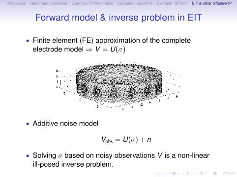
Forward model & inverse problem in EIT

• Finite element (FE) approximation of the completeelectrode model⇒ V = U(σ)

• Additive noise model

Vobs = U(σ) + n

• Solving σ based on noisy observations V is a non-linearill-posed inverse problem.


Example: EIT imaging of concrete

Figure: EIT imaging of concrete (Karhunen et al 2010)


Forward model & inverse problem in EIT

• EIT is a classical inverse problem; has been widely studiedtheoretically.

• Lot of applications:• Process industry (multi-phase flows, single-phase flows)• Geophysis (explosives, archeology, soil water content, ect)• Medical imaging (breast cancer, lungs, brains)• Concrete (cracks, reinforcing bars, humidity, etc)• etc

• In this course, many of the examples on large scaleinverse problems are related to EIT. Note however, thatmany of the methods are directly applicable to other largescale inverse problems.

Statistical and Computational Inverse Problems with ...

Documents

Transcript of Statistical and Computational Inverse Problems with ...