
Problems and Search - SRM · PDF fileProblems and Search ... • Ignorable problems can be...
192
Problems and Search Chapter 2
Transcript of Problems and Search - SRM · PDF fileProblems and Search ... • Ignorable problems can be...

Problems and Search
Chapter 2

Outline
• State space search
• Search strategies
• Problem characteristics
• Design of search programs
2
State Space Search
Problem solving = Searching for a goal state
3
State Space Search: Playing Chess
• Each position can be described by an 8‐by‐8
array.
• Initial position is the game opening position.
• Goal position is any position in which the opponent does not have a legal move and his or her king is under attack.
• Legal moves can be described by a set of rules:− Left sides are matched against the current state.− Right sides describe the new resulting state.
4
State Space Search: Playing Chess
• State space is a set of legal positions.
• Starting at the initial state.
• Using the set of rules to move from one state to another.
• Attempting to end up in a goal state.
5
State Space Search: Water Jug Problem
“You are given two jugs, a 4‐litre one and a 3‐litre one.
Neither has any measuring markers on it. There is a
pump that can be used to fill the jugs with water. How
can you get exactly 2 litres of water into 4‐litre jug.”
6

State Space Search: Water Jug Problem
• State: (x, y)
x = 0, 1, 2, 3, or 4 y = 0, 1, 2, 3
• Start state: (0, 0).
• Goal state: (2, n) for any n.
• Attempting to end up in a goal state.
7
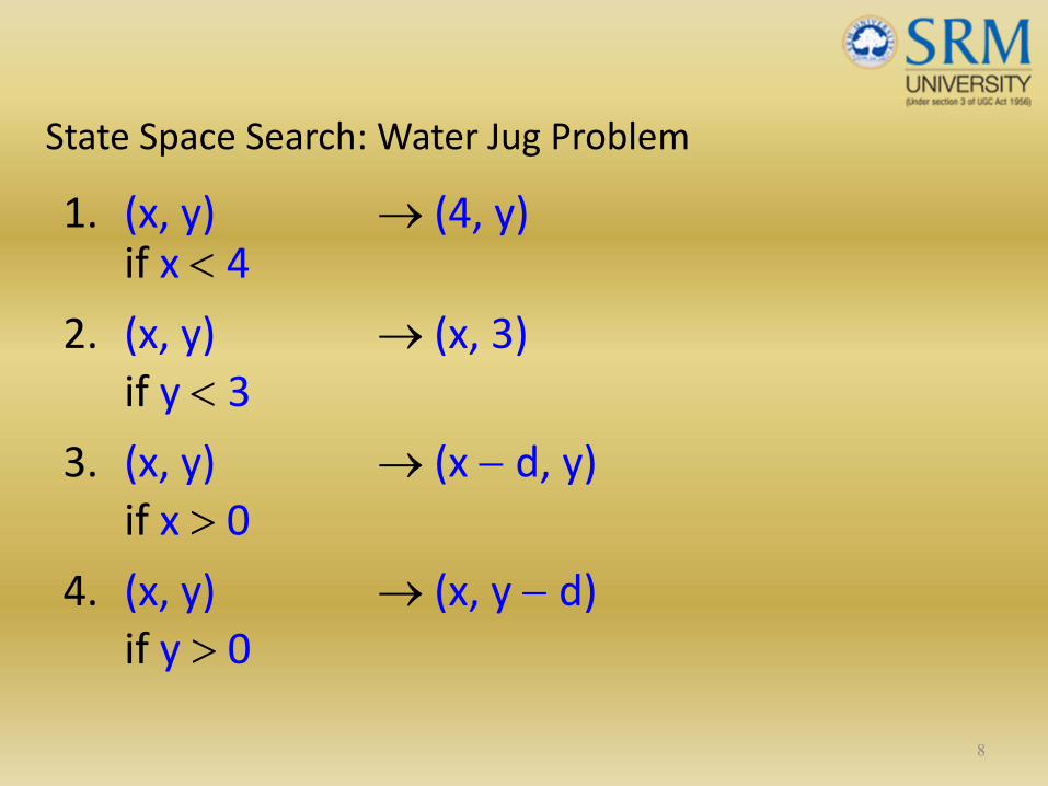
State Space Search: Water Jug Problem
1. (x, y) → (4, y)if x < 4
2. (x, y) → (x, 3)if y < 3
3. (x, y) → (x − d, y)if x > 0
4. (x, y) → (x, y − d)if y > 0
8

State Space Search: Water Jug Problem
5. (x, y) → (0, y)if x > 0
6. (x, y) → (x, 0)if y > 0
7. (x, y) → (4, y − (4 − x))if x + y ≥ 4, y > 0
8. (x, y) → (x − (3 − y), 3)if x + y ≥ 3, x > 0
9

State Space Search: Water Jug Problem
9. (x, y) → (x + y, 0)if x + y ≤ 4, y > 0
10.(x, y) → (0, x + y)if x + y ≤ 3, x > 0
11.(0, 2) → (2, 0)
12.(2, y) → (0, y)
10
State Space Search: Water Jug Problem
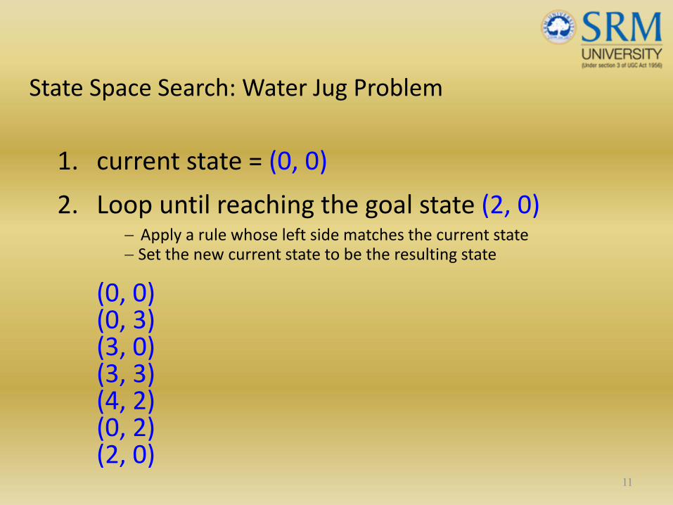
1. current state = (0, 0)
2. Loop until reaching the goal state (2, 0)− Apply a rule whose left side matches the current state− Set the new current state to be the resulting state
(0, 0)(0, 3)(3, 0)(3, 3)(4, 2)(0, 2)(2, 0)
11

State Space Search: Water Jug Problem
The role of the condition in the left side of a rule⇒ restrict the application of the rule⇒ more efficient
1. (x, y) → (4, y)if x < 4
2. (x, y) → (x, 3)if y < 3
12
State Space Search: Water Jug Problem
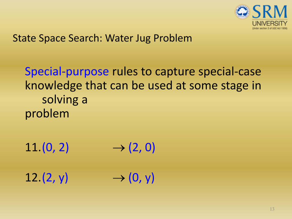
Special‐purpose rules to capture special‐case knowledge that can be used at some stage in
solving a problem
11.(0, 2) → (2, 0)
12.(2, y) → (0, y)
13
State Space Search: Summary
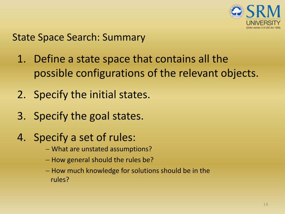
1. Define a state space that contains all the possible configurations of the relevant objects.
2. Specify the initial states.
3. Specify the goal states.
4. Specify a set of rules:− What are unstated assumptions?
− How general should the rules be?
− How much knowledge for solutions should be in the rules?
14

Search Strategies
Requirements of a good search strategy:
1. It causes motionOtherwise, it will never lead to a solution.
2. It is systematicOtherwise, it may use more steps than necessary.
3. It is efficientFind a good, but not necessarily the best, answer.
15

Search Strategies
1. Uninformed search (blind search)Having no information about the number of steps from the current state to the goal.
2. Informed search (heuristic search)More efficient than uninformed search.
16
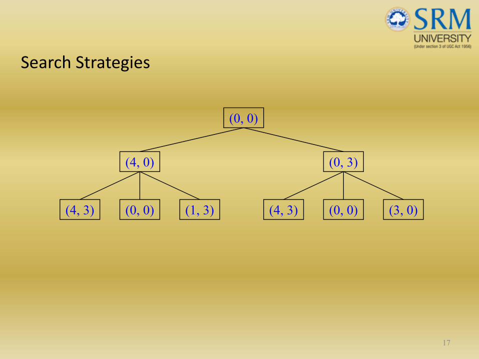
Search Strategies
17
(0, 0)
(4, 0) (0, 3)
(1, 3)(0, 0)(4, 3) (3, 0)(0, 0)(4, 3)
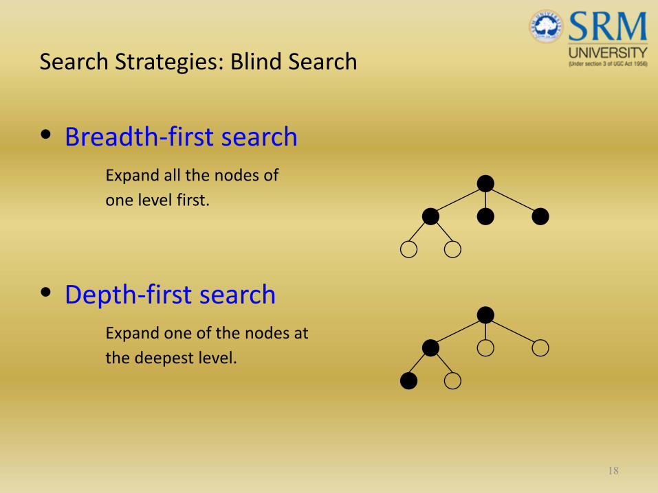
Search Strategies: Blind Search
• Breadth‐first searchExpand all the nodes of one level first.
• Depth‐first searchExpand one of the nodes at the deepest level.
18
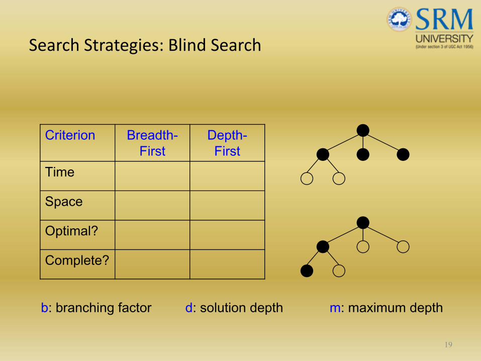
Search Strategies: Blind Search
19
Criterion Breadth-First
Depth-First
Time
Space
Optimal?
Complete?
b: branching factor d: solution depth m: maximum depth
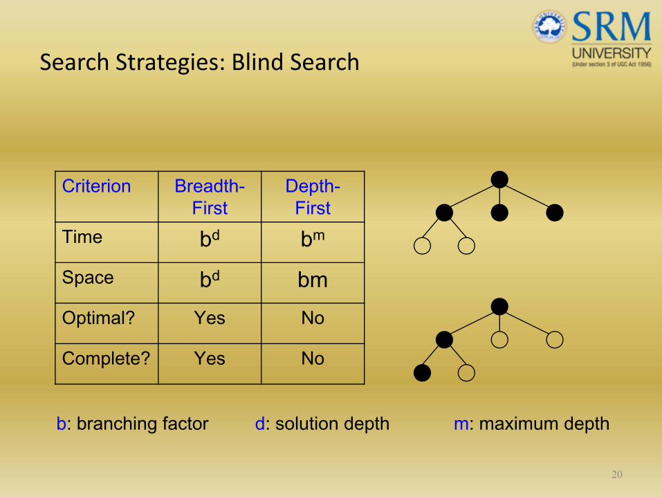
Search Strategies: Blind Search
20
Criterion Breadth-First
Depth-First
Time bd bm
Space bd bmOptimal? Yes No
Complete? Yes No
b: branching factor d: solution depth m: maximum depth
Search Strategies: Heuristic Search
• Heuristic: involving or serving as an aid to learning, discovery, or problem‐solving by experimental and especially trial‐and‐error methods. (Merriam‐Webster’s dictionary)
• Heuristic technique improves the efficiency of a search process, possibly by sacrificing claims of completeness or optimality.
21

Search Strategies: Heuristic Search
• Heuristic is for combinatorial explosion.
• Optimal solutions are rarely needed.
22
Search Strategies: Heuristic Search
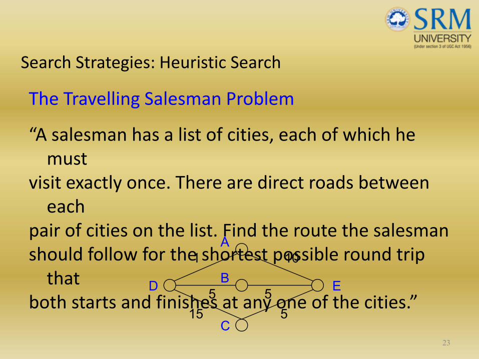
The Travelling Salesman Problem
“A salesman has a list of cities, each of which he must
visit exactly once. There are direct roads between each
pair of cities on the list. Find the route the salesman should follow for the shortest possible round trip that
both starts and finishes at any one of the cities.”
23
A
B
C
D E
1 10
5 5515
Search Strategies: Heuristic Search
Nearest neighbour heuristic:
1. Select a starting city.
2. Select the one closest to the current city.
3. Repeat step 2 until all cities have been visited.
24

Search Strategies: Heuristic Search
Nearest neighbour heuristic:
1. Select a starting city.
2. Select the one closest to the current city.
3. Repeat step 2 until all cities have been visited.
O(n2) vs. O(n!)
25
Search Strategies: Heuristic Search
• Heuristic function:
state descriptions → measures of desirability
26
Problem Characteristics
To choose an appropriate method for a particular problem:• Is the problem decomposable?• Can solution steps be ignored or undone?• Is the universe predictable?• Is a good solution absolute or relative?• Is the solution a state or a path?• What is the role of knowledge?• Does the task require human‐interaction?
27
Is the problem decomposable?
• Can the problem be broken down to smaller problems to be solved independently?
• Decomposable problem can be solved easily.
28
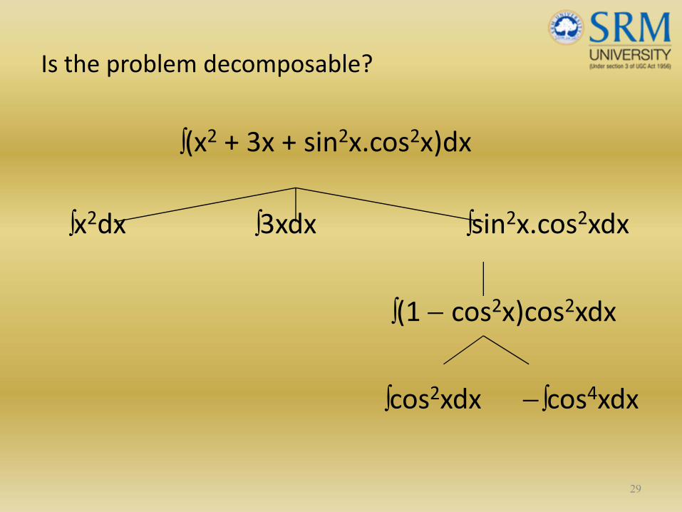
Is the problem decomposable?
∫(x2 + 3x + sin2x.cos2x)dx
∫x2dx ∫3xdx ∫sin2x.cos2xdx
∫(1 − cos2x)cos2xdx
∫cos2xdx −∫cos4xdx
29
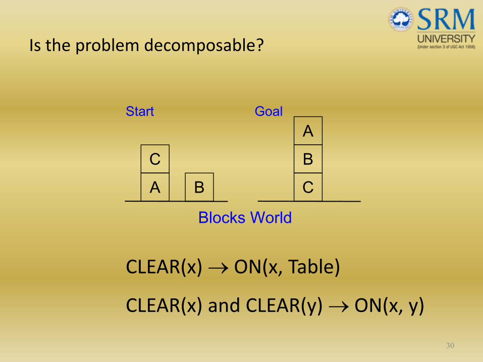
Is the problem decomposable?
CLEAR(x) → ON(x, Table)
CLEAR(x) and CLEAR(y) → ON(x, y)
30
AC
B CBA
Start Goal
Blocks World
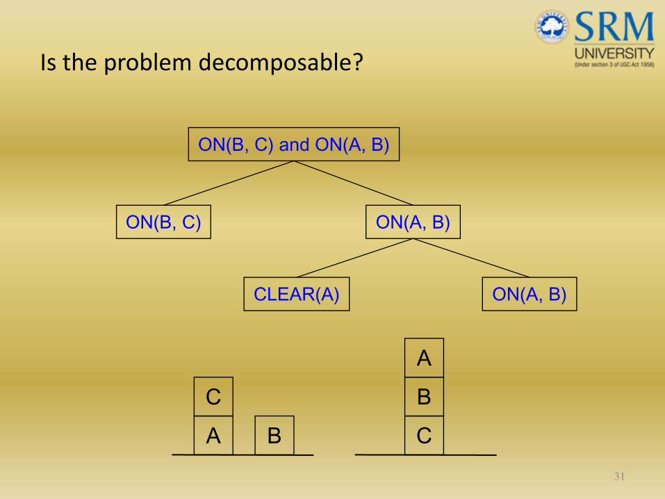
Is the problem decomposable?
31
ON(B, C) and ON(A, B)
ON(B, C) ON(A, B)
CLEAR(A) ON(A, B)
AC
B CBA
Can solution steps be ignored or undone?
Theorem Proving
A lemma that has been proved can be ignored for next
steps.
Ignorable!
32

Can solution steps be ignored or undone?
The 8‐Puzzle
Moves can be undone and backtracked.
Recoverable! 33
2 8 3
1 6 4
7 5
1 2 3
8 4
7 6 5
Can solution steps be ignored or undone?
Playing Chess
Moves cannot be retracted.
Irrecoverable!
34
Can solution steps be ignored or undone?
• Ignorable problems can be solved using a simple control structure that never backtracks.
• Recoverable problems can be solved using backtracking.
• Irrecoverable problems can be solved by recoverable style methods via planning.
35
Is the universe predictable?
The 8‐Puzzle
Every time we make a move, we know exactly what will
happen.
Certain outcome!
36

Is the universe predictable?
Playing Bridge
We cannot know exactly where all the cards are or what
the other players will do on their turns.
Uncertain outcome!
37
Is the universe predictable?
• For certain‐outcome problems, planning can used to generate a sequence of operators that is guaranteed to lead to a solution.
• For uncertain‐outcome problems, a sequence of generated operators can only have a good probability of leading to a solution.
Plan revision is made as the plan is carried out and the necessary feedback is provided.
38
Is a good solution absolute or relative?
1. Marcus was a man.
2. Marcus was a Pompeian.
3. Marcus was born in 40 A.D.
4. All men are mortal.
5. All Pompeians died when the volcano erupted in 79 A.D.
6. No mortal lives longer than 150 years.
7. It is now 2004 A.D.39

Is a good solution absolute or relative?
1. Marcus was a man.
2. Marcus was a Pompeian.
3. Marcus was born in 40 A.D.
4. All men are mortal.
5. All Pompeians died when the volcano erupted in 79 A.D.
6. No mortal lives longer than 150 years.
7. It is now 2004 A.D.
Is Marcus alive?
40
Is a good solution absolute or relative?
1. Marcus was a man.2. Marcus was a Pompeian.3. Marcus was born in 40 A.D.4. All men are mortal.5. All Pompeians died when the volcano
erupted in 79 A.D.6. No mortal lives longer than 150 years.7. It is now 2004 A.D.
Is Marcus alive?Different reasoning paths lead to the answer.
It does not matter which path we follow. 41
Is a good solution absolute or relative?
The Travelling Salesman Problem
We have to try all paths to find the shortest one.
42
Is a good solution absolute or relative?
• Any‐path problems can be solved using heuristics that suggest good paths to explore.
• For best‐path problems, much more exhaustive search will be performed.
43
Is the solution a state or a path?
Finding a consistent intepretation“The bank president ate a dish of pasta salad with
the fork”.
– “bank” refers to a financial situation or to a side of a river?
– “dish” or “pasta salad” was eaten?– Does “pasta salad” contain pasta, as “dog food” does not contain “dog”?
– Which part of the sentence does “with the fork” modify?What if “with vegetables” is there?
44
Is the solution a state or a path?
The Water Jug Problem
The path that leads to the goal must be reported.
45
Is the solution a state or a path?
• A path‐solution problem can be reformulated as a state‐solution problem by describing a state as a partial path to a solution.
• The question is whether that is natural or not.
46
What is the role of knowledge
Playing ChessKnowledge is important only to constrain the search for
a solution.
Reading NewspaperKnowledge is required even to be able to recognize a
solution.
47

Does the task require human‐interaction?
• Solitary problem, in which there is no intermediate communication and no demand for an explanation of the reasoning process.
• Conversational problem, in which intermediate communication is to provide either additional assistance to the computer or additional information to the user.
48

Problem Classification
• There is a variety of problem‐solving methods, but there is no one single way of solving all problems.
• Not all new problems should be considered as totally new. Solutions of similar problems can be exploited.
49

Homework
Exercises 1‐7 (Chapter 2 – AI Rich & Knight)
50

51

Heuristic Search
Chapter 3

Outline
• Generate‐and‐test
• Hill climbing
• Best‐first search
• Problem reduction
• Constraint satisfaction
• Means‐ends analysis
53
Generate‐and‐Test
Algorithm1. Generate a possible solution.
2. Test to see if this is actually a solution.
3. Quit if a solution has been found. Otherwise, return to step 1.
54
Generate‐and‐Test
• Acceptable for simple problems.
• Inefficient for problems with large space.
55
Generate‐and‐Test
• Exhaustive generate‐and‐test.
• Heuristic generate‐and‐test: not consider paths that seem unlikely to lead to a solution.
• Plan generate‐test:− Create a list of candidates.
− Apply generate‐and‐test to that list.
56
Generate‐and‐Test
Example: coloured blocks“Arrange four 6‐sided cubes in a row, with each
side of each cube painted one of four colours, such
that on all four sides of the row one block face of each colour is
showing.”
57

Generate‐and‐Test
Example: coloured blocks
Heuristic: if there are more red faces than other colours
then, when placing a block with several redfaces, use few
of them as possible as outside faces.
58

Hill Climbing
• Searching for a goal state = Climbing to the
top of a hill
59

Hill Climbing
• Generate‐and‐test + direction to move.
• Heuristic function to estimate how close a given state is to a goal state.
60
Simple Hill Climbing
Algorithm1. Evaluate the initial state.
2. Loop until a solution is found or there are no new operators left to be applied:
− Select and apply a new operator− Evaluate the new state:
goal → quitbetter than current state → new current state
61
Simple Hill Climbing
• Evaluation function as a way to inject task‐specific knowledge into the control process.
62

Simple Hill Climbing
Example: coloured blocks
Heuristic function: the sum of the number of different
colours on each of the four sides (solution = 16).
63
Steepest‐Ascent Hill Climbing (Gradient Search)
• Considers all the moves from the current
state.
• Selects the best one as the next state.
64
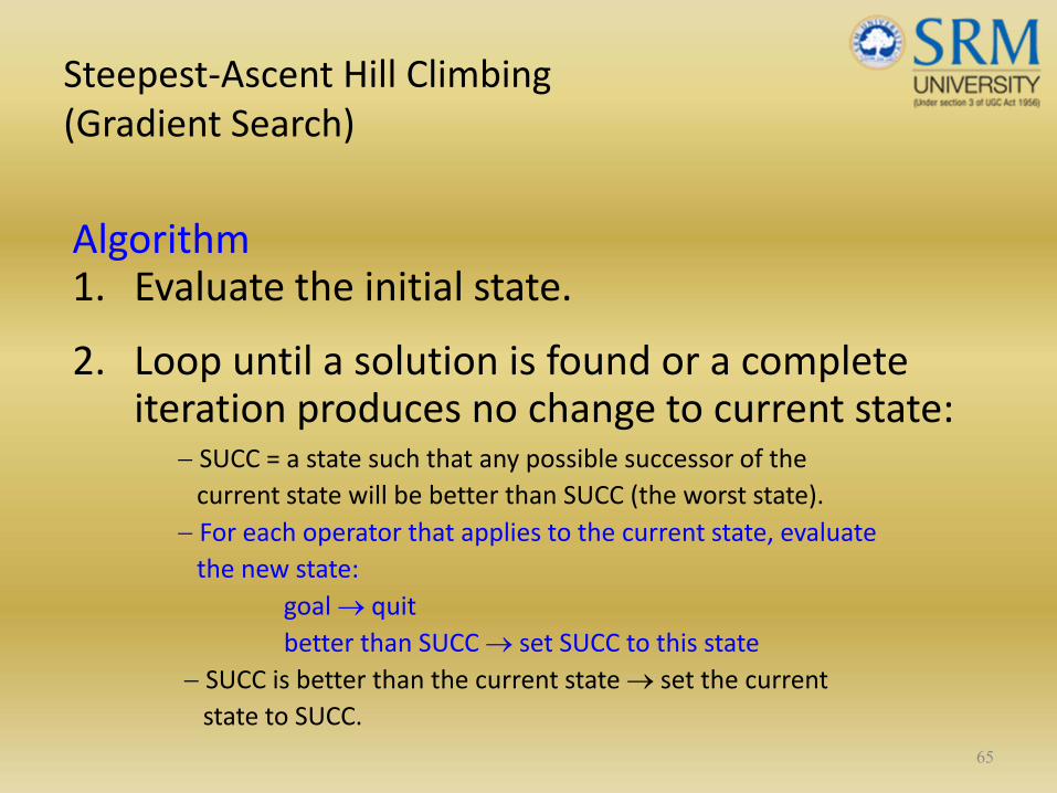
Steepest‐Ascent Hill Climbing (Gradient Search)
Algorithm1. Evaluate the initial state.
2. Loop until a solution is found or a complete iteration produces no change to current state:
− SUCC = a state such that any possible successor of the current state will be better than SUCC (the worst state).
− For each operator that applies to the current state, evaluate the new state:
goal → quitbetter than SUCC → set SUCC to this state
− SUCC is better than the current state → set the current state to SUCC.
65

Hill Climbing: Disadvantages
Local maximumA state that is better than all of its neighbours, but not
better than some other states far away.
66
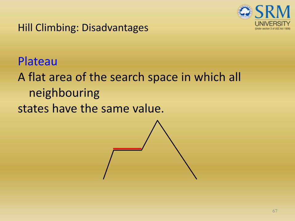
Hill Climbing: Disadvantages
PlateauA flat area of the search space in which all neighbouring
states have the same value.
67

Hill Climbing: Disadvantages
RidgeThe orientation of the high region, compared to the set
of available moves, makes it impossible to climb up.
However, two moves executed serially may increase
the height.
68
Hill Climbing: Disadvantages
Ways Out
• Backtrack to some earlier node and try going in a different direction.
• Make a big jump to try to get in a new section.
• Moving in several directions at once.
69

Hill Climbing: Disadvantages
• Hill climbing is a local method: Decides what to do next by looking only at the “immediate” consequences of its choices.
• Global information might be encoded in heuristic functions.
70

Hill Climbing: Disadvantages
71
BCD
ABC
Start Goal
Blocks World
A D
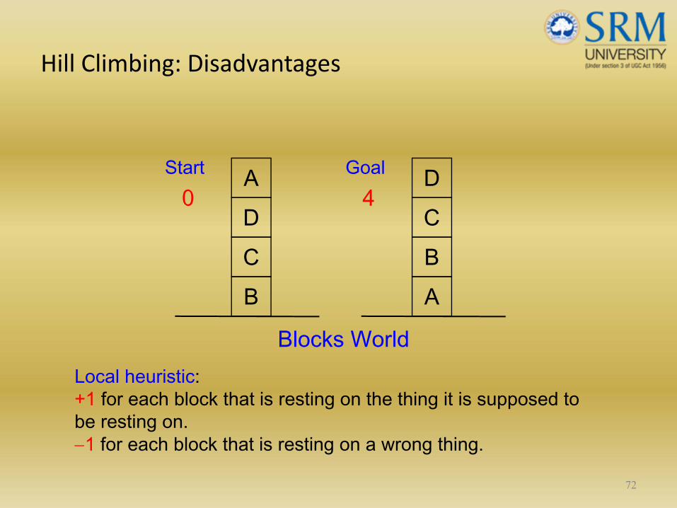
Hill Climbing: Disadvantages
72
BCD
ABC
Start Goal
Blocks World
A D
Local heuristic: +1 for each block that is resting on the thing it is supposed to be resting on. −1 for each block that is resting on a wrong thing.
0 4

Hill Climbing: Disadvantages
73
BCD
BCD
A
A0 2

Hill Climbing: Disadvantages
74
BCDA
BC D
A BC
DA
00
0
BCD
A
2
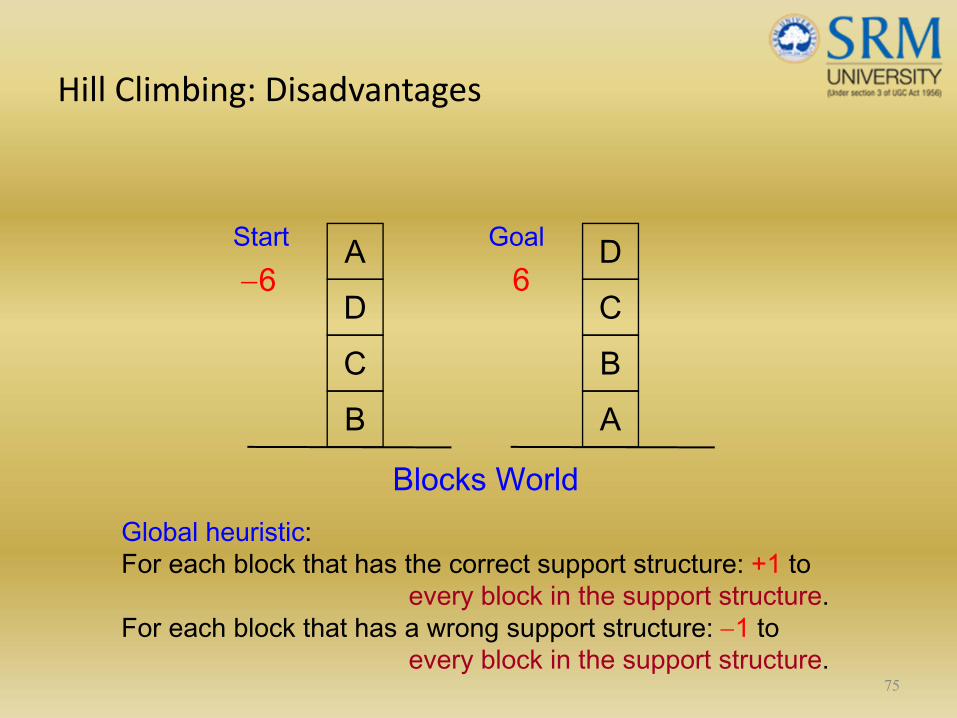
Hill Climbing: Disadvantages
75
BCD
ABC
Start Goal
Blocks World
A D
Global heuristic: For each block that has the correct support structure: +1 to
every block in the support structure. For each block that has a wrong support structure: −1 to
every block in the support structure.
−6 6
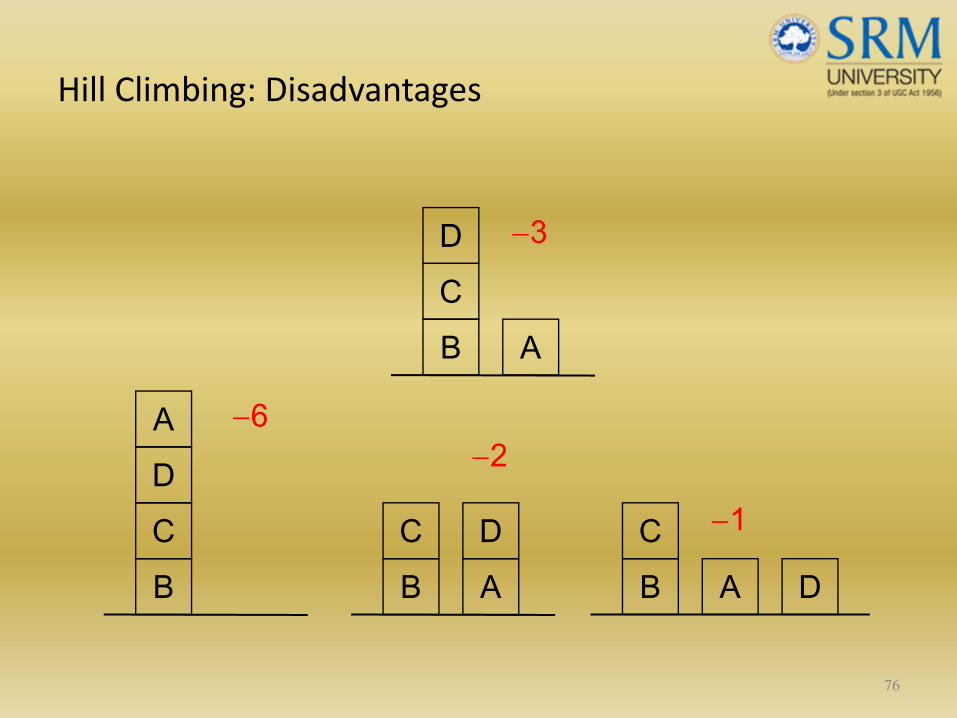
Hill Climbing: Disadvantages
76
BCDA
BC D
A BC
DA
−6−2
−1
BCD
A
−3

Hill Climbing: Conclusion
• Can be very inefficient in a large, rough problem space.
• Global heuristic may have to pay for computational complexity.
• Often useful when combined with other methods, getting it started right in the right general neighbourhood.
77
Simulated Annealing
• A variation of hill climbing in which, at the beginning of the process, some downhill movesmay be made.
• To do enough exploration of the whole spaceearly on, so that the final solution is relatively insensitive to the starting state.
• Lowering the chances of getting caught at a local maximum, or plateau, or a ridge.
78
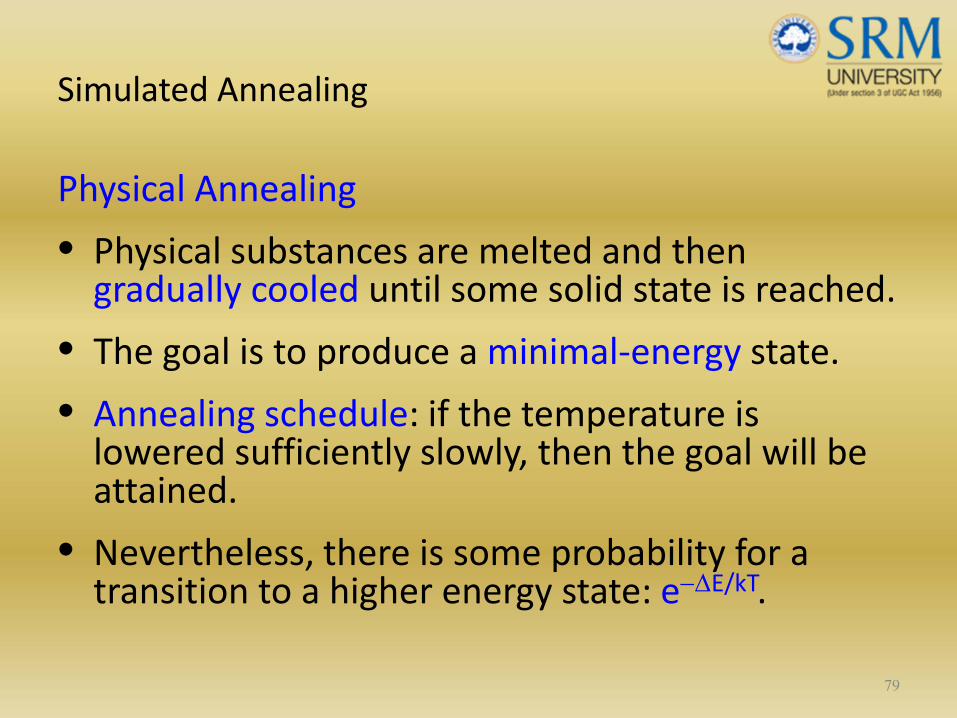
Simulated Annealing
Physical Annealing
• Physical substances are melted and then gradually cooled until some solid state is reached.
• The goal is to produce a minimal‐energy state.
• Annealing schedule: if the temperature is lowered sufficiently slowly, then the goal will be attained.
• Nevertheless, there is some probability for a transition to a higher energy state: e−ΔE/kT.
79

Simulated Annealing
Algorithm1. Evaluate the initial state.
2. Loop until a solution is found or there are no new operators left to be applied:
− Set T according to an annealing schedule
− Selects and applies a new operator
− Evaluate the new state:
goal → quit
ΔE = Val(current state) − Val(new state)
ΔE < 0 → new current state80
Best‐First Search
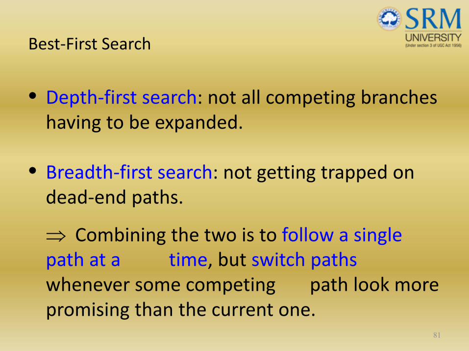
• Depth‐first search: not all competing branches having to be expanded.
• Breadth‐first search: not getting trapped on dead‐end paths.
⇒ Combining the two is to follow a single path at a time, but switch pathswhenever some competing path look more promising than the current one.
81
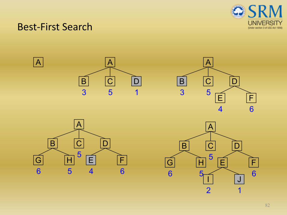
Best‐First Search
82
A
DCB
FEHG
JI
5
66 5
2 1
A
DCB
FEHG5
66 5 4
A
DCB
FE5
6
3
4
A
DCB53 1
A
Best‐First Search
• OPEN: nodes that have been generated, but have not examined.
This is organized as a priority queue.
• CLOSED: nodes that have already been examined.
Whenever a new node is generated, checkwhether it has been generated before.
83
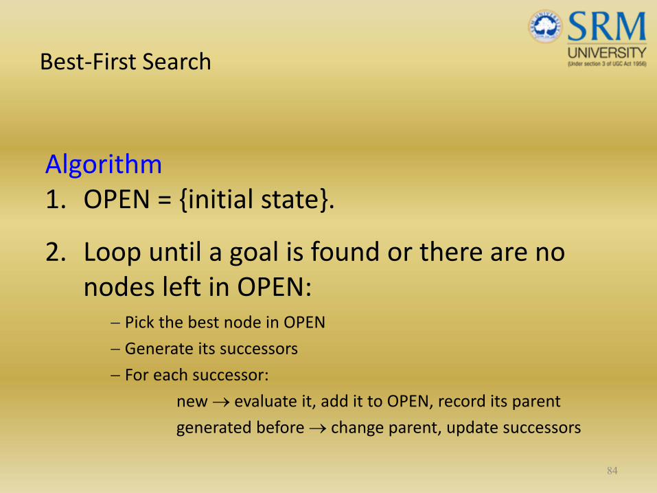
Best‐First Search
Algorithm1. OPEN = {initial state}.
2. Loop until a goal is found or there are no nodes left in OPEN:
− Pick the best node in OPEN
− Generate its successors
− For each successor:
new → evaluate it, add it to OPEN, record its parent
generated before → change parent, update successors
84

Best‐First Search
• Greedy search:h(n) = estimated cost of the cheapest path from node n to a goal state.
85
Best‐First Search
• Uniform‐cost search:g(n) = cost of the cheapest path from the initial state to node n.
86
Best‐First Search
• Greedy search:h(n) = estimated cost of the cheapest path from node n to a goal state.
Neither optimal nor complete
87
Best‐First Search
• Greedy search:h(n) = estimated cost of the cheapest path from node n to a goal state.
Neither optimal nor complete
• Uniform‐cost search:g(n) = cost of the cheapest path from the initial state to node n.
Optimal and complete, but very inefficient88
Best‐First Search
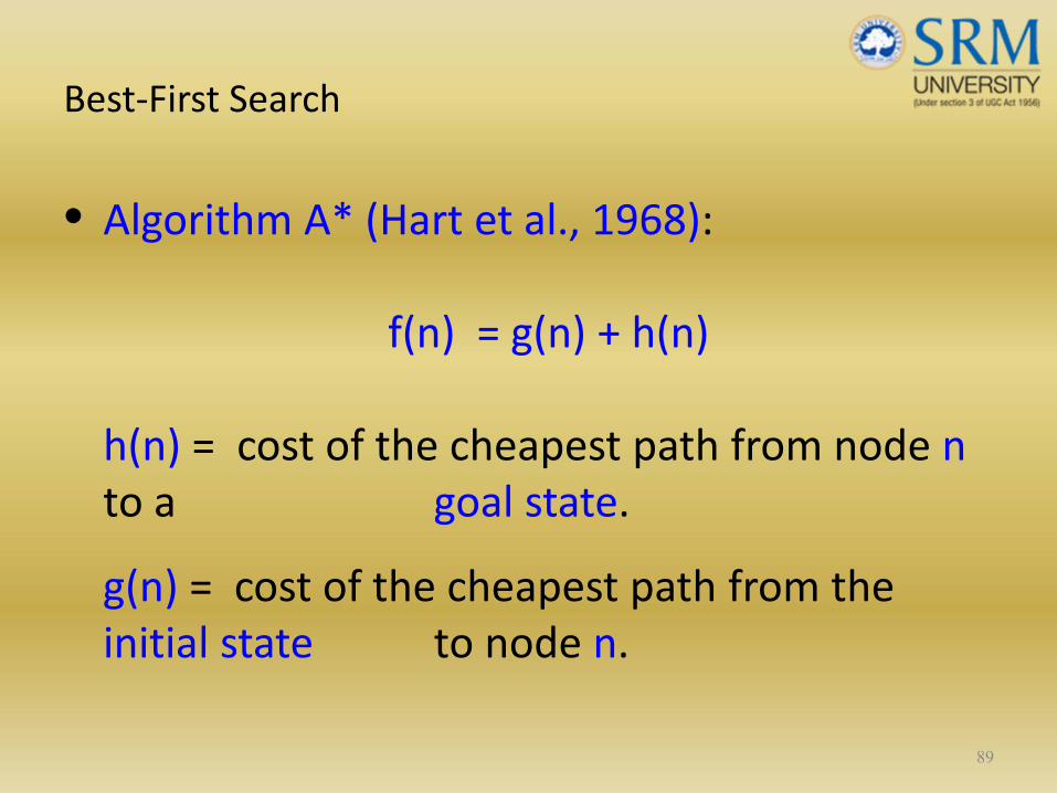
• Algorithm A* (Hart et al., 1968):
f(n) = g(n) + h(n)
h(n) = cost of the cheapest path from node nto a goal state.
g(n) = cost of the cheapest path from the initial state to node n.
89
Best‐First Search
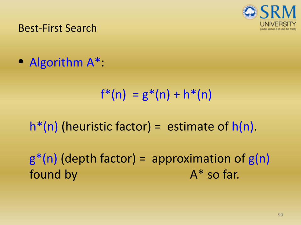
• Algorithm A*:
f*(n) = g*(n) + h*(n)
h*(n) (heuristic factor) = estimate of h(n).
g*(n) (depth factor) = approximation of g(n)found by A* so far.
90

Problem Reduction
91
Goal: Acquire TV set
AND-OR Graphs
Goal: Steal TV set Goal: Earn some money Goal: Buy TV set
Algorithm AO* (Martelli & Montanari 1973, Nilsson 1980)
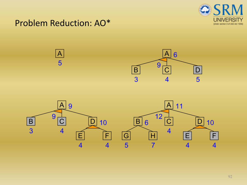
Problem Reduction: AO*
92
A
DCB43 5
A5
6
FE44
A
DCB43
10
9
9
9
FE44
A
DCB4
6 10
1112
HG75

Problem Reduction: AO*
93
A
G
CB 10
5
11
13
ED 65 F 3
A
G
CB 15
10
14
13
ED 65 F 3
H 9Necessary backward propagation
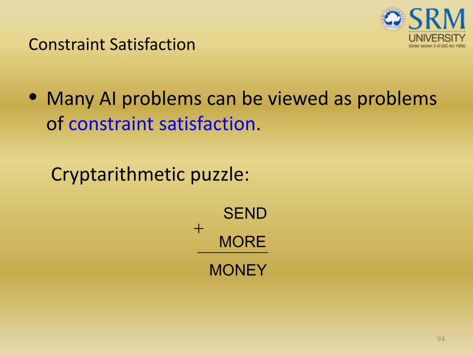
Constraint Satisfaction
• Many AI problems can be viewed as problems of constraint satisfaction.
Cryptarithmetic puzzle:
94
SEND
MORE
MONEY
+

Constraint Satisfaction
• As compared with a straightforard searchprocedure, viewing a problem as one of constraint satisfaction can reduce substantially the amount of search.
95
Constraint Satisfaction
• Operates in a space of constraint sets.
• Initial state contains the original constraintsgiven in the problem.
• A goal state is any state that has been constrained “enough”.
96
Constraint Satisfaction
Two‐step process:
1. Constraints are discovered and propagated as far as possible.
2. If there is still not a solution, then search begins, adding new constraints.
97
98
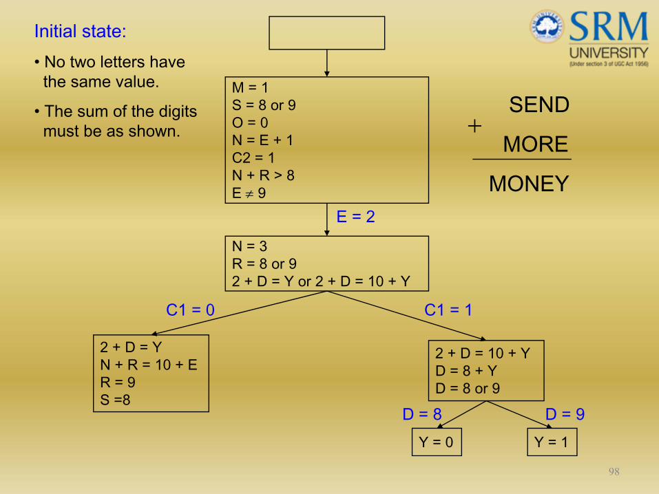
M = 1S = 8 or 9O = 0N = E + 1C2 = 1N + R > 8E ≠ 9
N = 3R = 8 or 92 + D = Y or 2 + D = 10 + Y
2 + D = YN + R = 10 + ER = 9S =8
2 + D = 10 + YD = 8 + YD = 8 or 9
Y = 0 Y = 1
E = 2
C1 = 0 C1 = 1
D = 8 D = 9
Initial state:• No two letters have the same value.
• The sum of the digits must be as shown.
SEND
MORE
MONEY
+
Constraint Satisfaction
Two kinds of rules:
1. Rules that define valid constraint propagation.
2. Rules that suggest guesses when necessary.
99
Homework
Exercises 1‐14 (Chapter 3 – AI Rich & Knight)
Reading Algorithm A*
(http://en.wikipedia.org/wiki/A%2A_algorithm)
100

101

Game Playing
Chapter 8

Outline
• Overview
• Minimax search
• Adding alpha‐beta cutoffs
• Additional refinements
• Iterative deepening
• Specific games
103
Overview
Old beliefs
Games provided a structured task in which it was very easy to measure success or failure.
Games did not obviously require large amounts of knowledge, thought to be solvable by straightforward search.
104
Overview
Chess
The average branching factor is around 35.
In an average game, each player might make 50 moves.
One would have to examine 35100 positions.
105
Overview
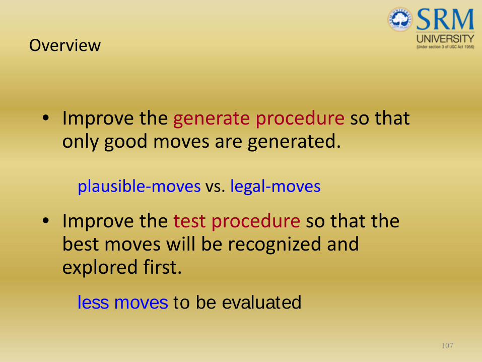
• Improve the generate procedure so that only good moves are generated.
• Improve the test procedure so that the best moves will be recognized and explored first.
106
Overview
• Improve the generate procedure so that only good moves are generated.
plausible‐moves vs. legal‐moves
• Improve the test procedure so that the best moves will be recognized and explored first.
less moves to be evaluated
107
Overview
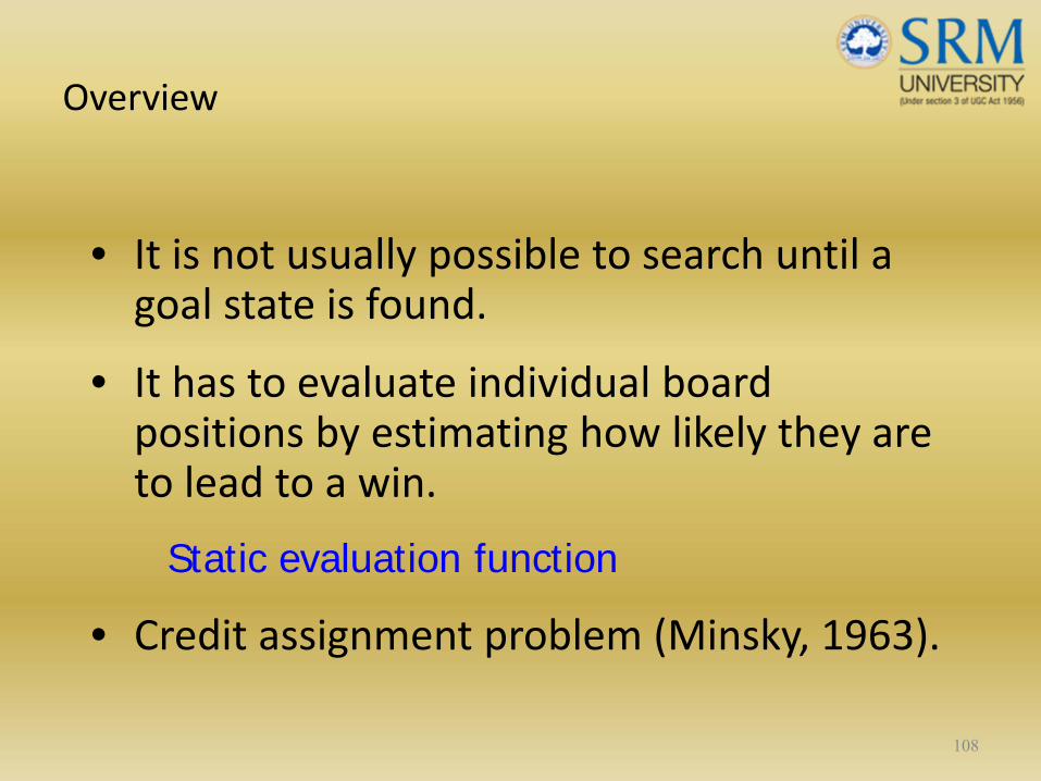
• It is not usually possible to search until a goal state is found.
• It has to evaluate individual board positions by estimating how likely they are to lead to a win.
Static evaluation function
• Credit assignment problem (Minsky, 1963).
108

Overview
• Good plausible‐move generator.
• Good static evaluation function.
109
Minimax Search
• Depth‐first and depth‐limited search.
• At the player choice, maximize the static evaluation of the next position.
• At the opponent choice, minimize the static evaluation of the next position.
110
Minimax Search
111
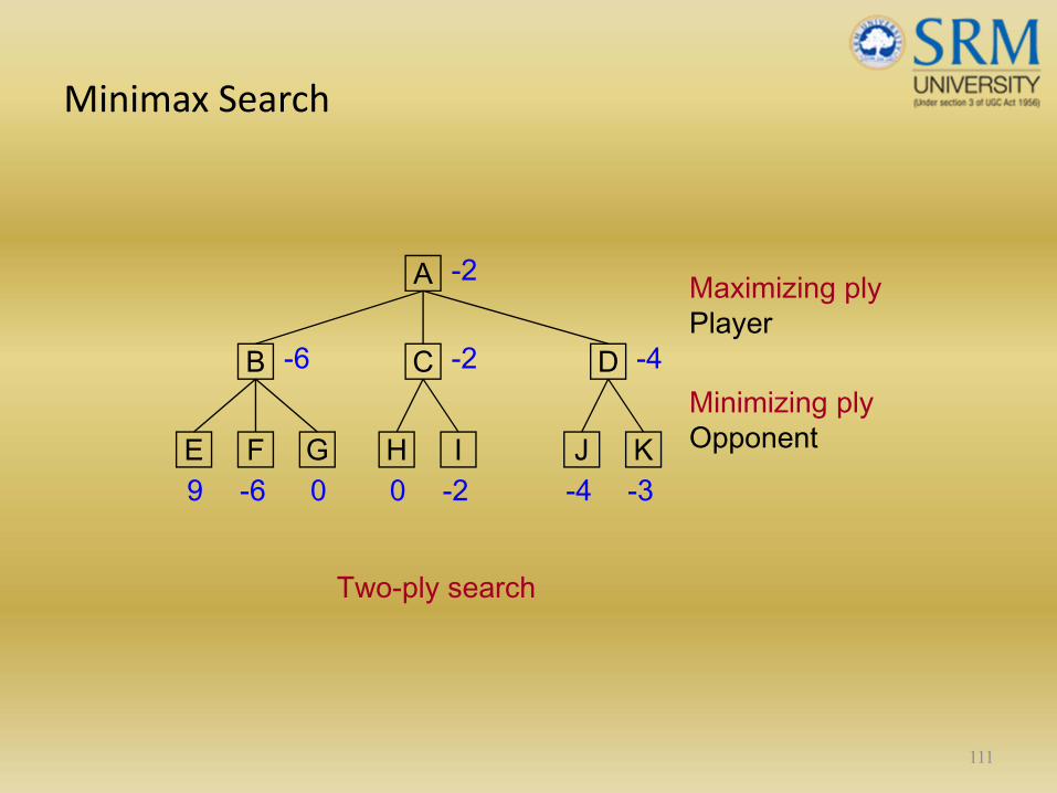
A
DCB
JFE09 -6 0G KH I
-2 -3-4
-6 -2 -4
-2 Maximizing plyPlayer
Minimizing plyOpponent
Two-ply search

Minimax Search
Player(Position, Depth):for each S ∈ SUCCESSORS(Position) do
RESULT = Opponent(S, Depth + 1)
NEW‐VALUE = VALUE(RESULT)
if NEW-VALUE > MAX-SCORE, thenMAX‐SCORE = NEW‐VALUE
BEST‐PATH = PATH(RESULT) + S
returnVALUE = MAX‐SCORE
PATH = BEST‐PATH
112
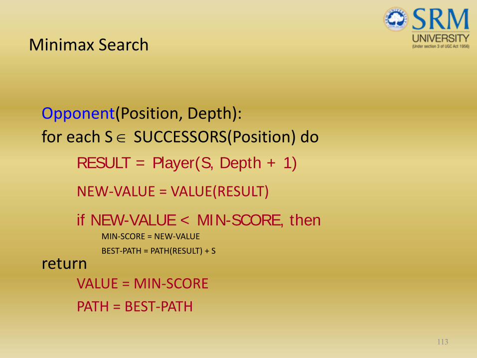
Minimax Search
Opponent(Position, Depth):for each S ∈ SUCCESSORS(Position) do
RESULT = Player(S, Depth + 1)
NEW‐VALUE = VALUE(RESULT)
if NEW-VALUE < MIN-SCORE, thenMIN‐SCORE = NEW‐VALUE
BEST‐PATH = PATH(RESULT) + S
returnVALUE = MIN‐SCORE
PATH = BEST‐PATH
113
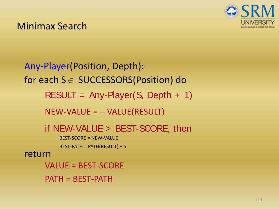
Minimax Search
Any‐Player(Position, Depth):for each S ∈ SUCCESSORS(Position) do
RESULT = Any-Player(S, Depth + 1)
NEW‐VALUE = − VALUE(RESULT)
if NEW-VALUE > BEST-SCORE, thenBEST‐SCORE = NEW‐VALUE
BEST‐PATH = PATH(RESULT) + S
returnVALUE = BEST‐SCORE
PATH = BEST‐PATH
114
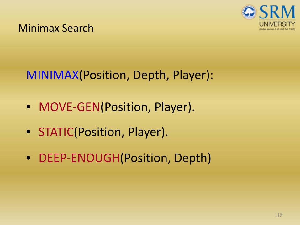
Minimax Search
MINIMAX(Position, Depth, Player):
• MOVE‐GEN(Position, Player).
• STATIC(Position, Player).
• DEEP‐ENOUGH(Position, Depth)
115
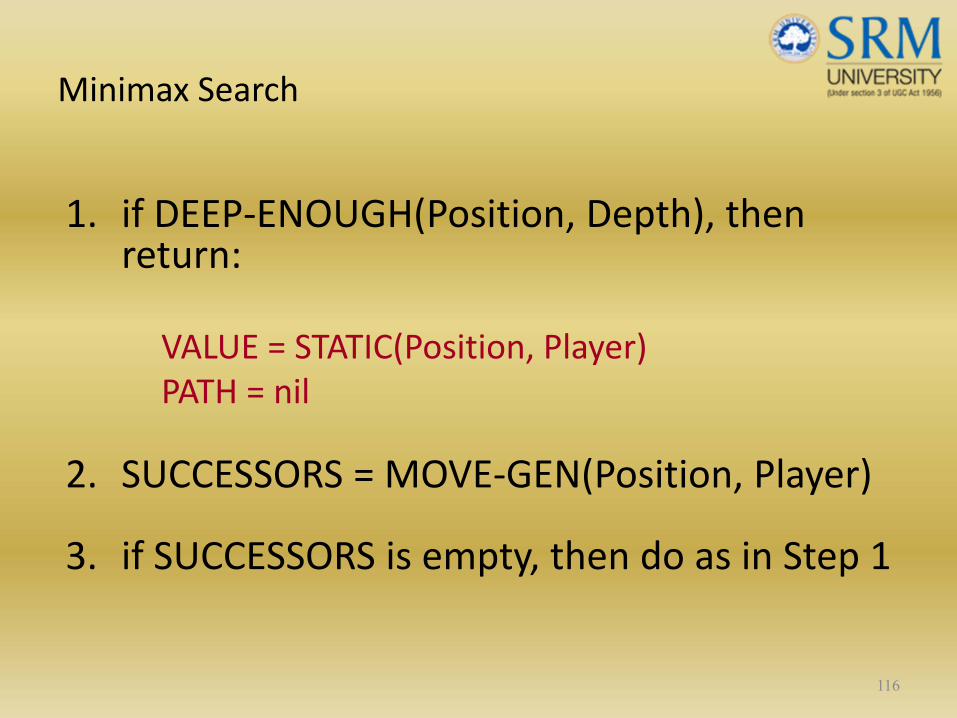
Minimax Search
1. if DEEP‐ENOUGH(Position, Depth), then return:
VALUE = STATIC(Position, Player)PATH = nil
2. SUCCESSORS = MOVE‐GEN(Position, Player)
3. if SUCCESSORS is empty, then do as in Step 1
116

Minimax Search
4. if SUCCESSORS is not empty:RESULT‐SUCC = MINIMAX(SUCC, Depth+1, Opp(Player))
NEW‐VALUE = - VALUE(RESULT‐SUCC)if NEW‐VALUE > BEST‐SCORE, then:
BEST‐SCORE = NEW‐VALUE
BEST‐PATH = PATH(RESULT‐SUCC) + SUCC
5. Return:VALUE = BEST‐SCORE
PATH = BEST‐PATH
117
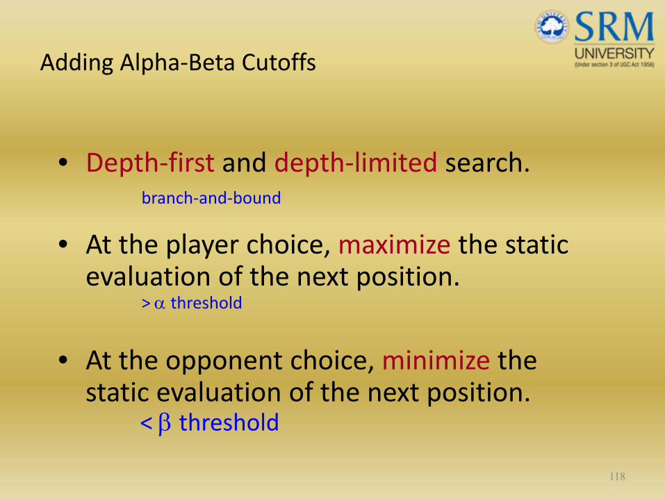
Adding Alpha‐Beta Cutoffs
• Depth‐first and depth‐limited search.branch‐and‐bound
• At the player choice, maximize the static evaluation of the next position.
> α threshold
• At the opponent choice, minimize the static evaluation of the next position.
< β threshold
118

Adding Alpha‐Beta Cutoffs
119
A
CB
ED3 5 -5
F G
3> 3 Maximizing ply
Player
Minimizing plyOpponent
Alpha cutoffs
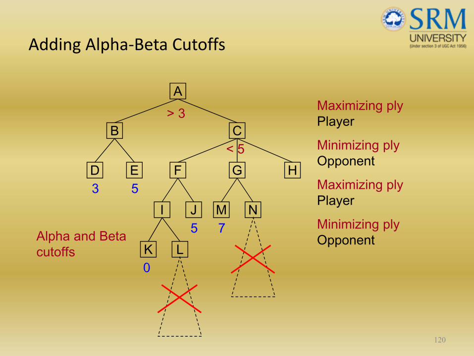
Adding Alpha‐Beta Cutoffs
120
A
CB
ED3 5
> 3
F G
Maximizing plyPlayer
Minimizing plyOpponent
Alpha and Beta cutoffs
H
JI5
NM
LK0
< 5
7
Maximizing plyPlayer
Minimizing plyOpponent
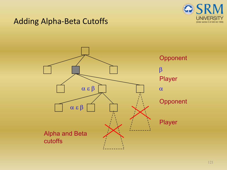
Adding Alpha‐Beta Cutoffs
121
Opponent
Player
Alpha and Beta cutoffs
Opponent
Player
β
α ε β α
α ε β
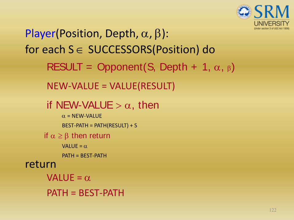
Player(Position, Depth, α, β):for each S ∈ SUCCESSORS(Position) do
RESULT = Opponent(S, Depth + 1, α, β)
NEW‐VALUE = VALUE(RESULT)
if NEW-VALUE > α, thenα = NEW‐VALUE
BEST‐PATH = PATH(RESULT) + S
if α ≥ β then returnVALUE = α
PATH = BEST‐PATH
returnVALUE = αPATH = BEST‐PATH
122
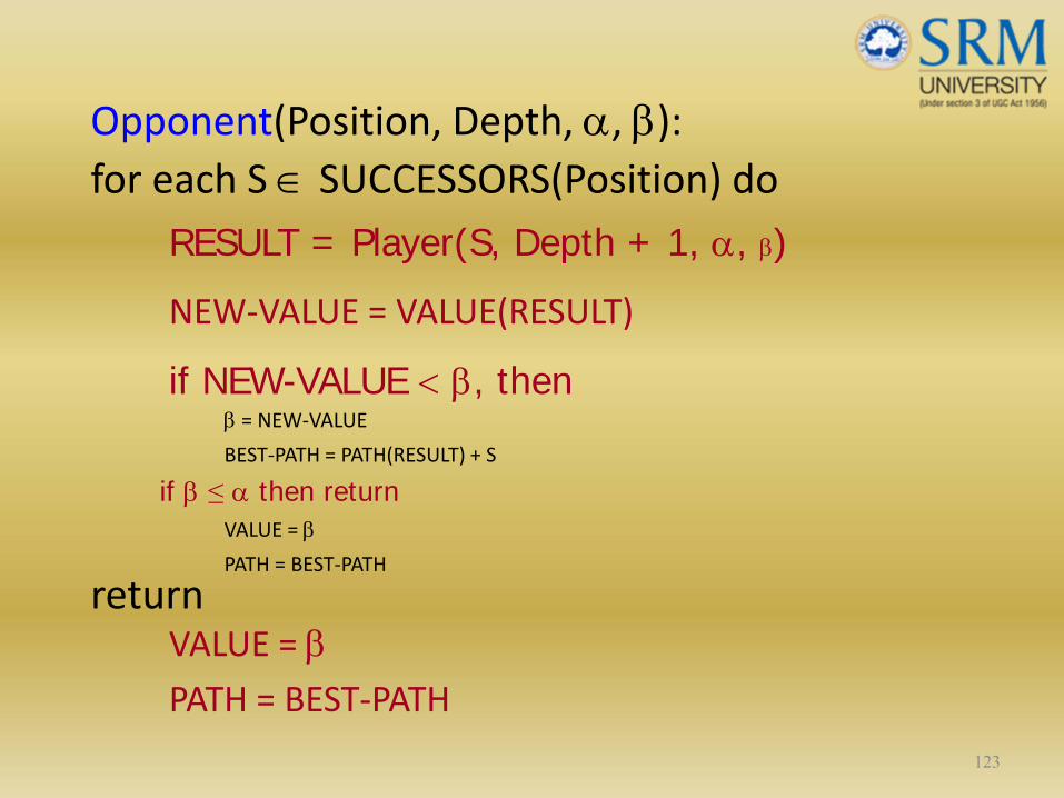
Opponent(Position, Depth, α, β):for each S ∈ SUCCESSORS(Position) do
RESULT = Player(S, Depth + 1, α, β)
NEW‐VALUE = VALUE(RESULT)
if NEW-VALUE < β, thenβ = NEW‐VALUE
BEST‐PATH = PATH(RESULT) + S
if β ≤ α then returnVALUE = β
PATH = BEST‐PATH
returnVALUE = βPATH = BEST‐PATH
123

Any‐Player(Position, Depth, α, β):for each S ∈ SUCCESSORS(Position) do
RESULT = Any-Player(S, Depth + 1, −β, −α)
NEW‐VALUE = − VALUE(RESULT)
if NEW-VALUE > α, thenα = NEW‐VALUE
BEST‐PATH = PATH(RESULT) + S
if α ≥ β then returnVALUE = α
PATH = BEST‐PATH
returnVALUE = αPATH = BEST‐PATH
124
Adding Alpha‐Beta Cutoffs
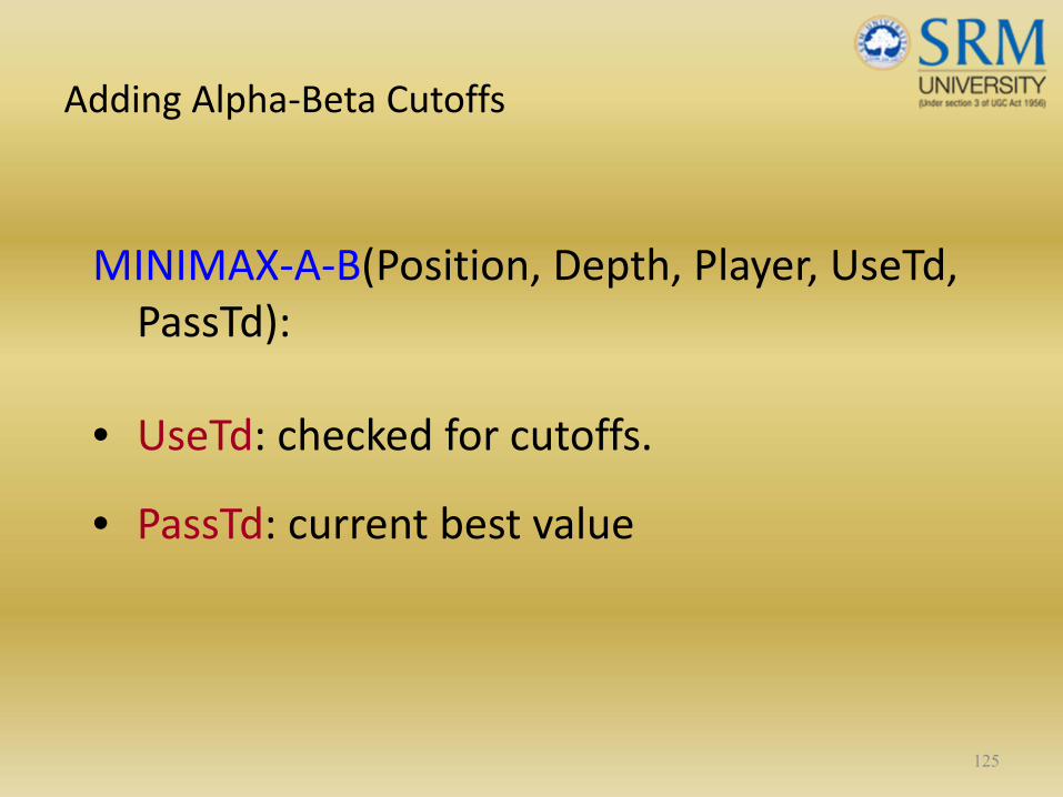
MINIMAX‐A‐B(Position, Depth, Player, UseTd, PassTd):
• UseTd: checked for cutoffs.
• PassTd: current best value
125

Adding Alpha‐Beta Cutoffs
1. if DEEP‐ENOUGH(Position, Depth), then return:
VALUE = STATIC(Position, Player)PATH = nil
2. SUCCESSORS = MOVE‐GEN(Position, Player)
3. if SUCCESSORS is empty, then do as in Step 1
126
Adding Alpha‐Beta Cutoffs
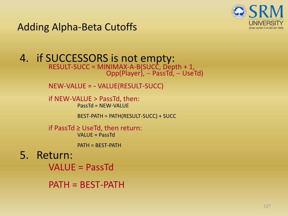
4. if SUCCESSORS is not empty:RESULT‐SUCC = MINIMAX‐A‐B(SUCC, Depth + 1,
Opp(Player), − PassTd, − UseTd)
NEW‐VALUE = - VALUE(RESULT‐SUCC)if NEW‐VALUE > PassTd, then:
PassTd = NEW‐VALUE
BEST‐PATH = PATH(RESULT‐SUCC) + SUCC
if PassTd ≥ UseTd, then return:VALUE = PassTd
PATH = BEST‐PATH
5. Return:VALUE = PassTd
PATH = BEST‐PATH
127

Additional Refinements
• Futility cutoffs
• Waiting for quiescence
• Secondary search
• Using book moves
• Not assuming opponent’s optimal move
128
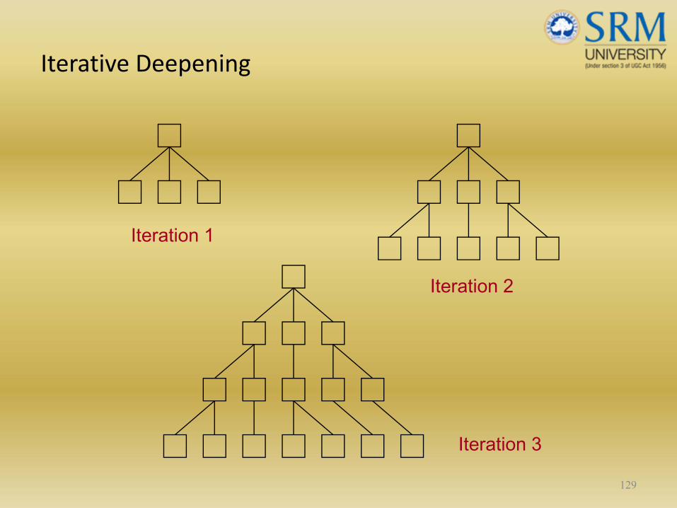
Iterative Deepening
129
Iteration 1
Iteration 2
Iteration 3

Iterative Deepening
• Search can be aborted at any time and the best move of the previous iteration is chosen.
• Previous iterations can provide invaluable move‐ordering constraints.
130
Iterative Deepening
• Can be adapted for single‐agent search.
• Can be used to combine the best aspects of depth‐first search and breadth‐first search.
131
Iterative Deepening
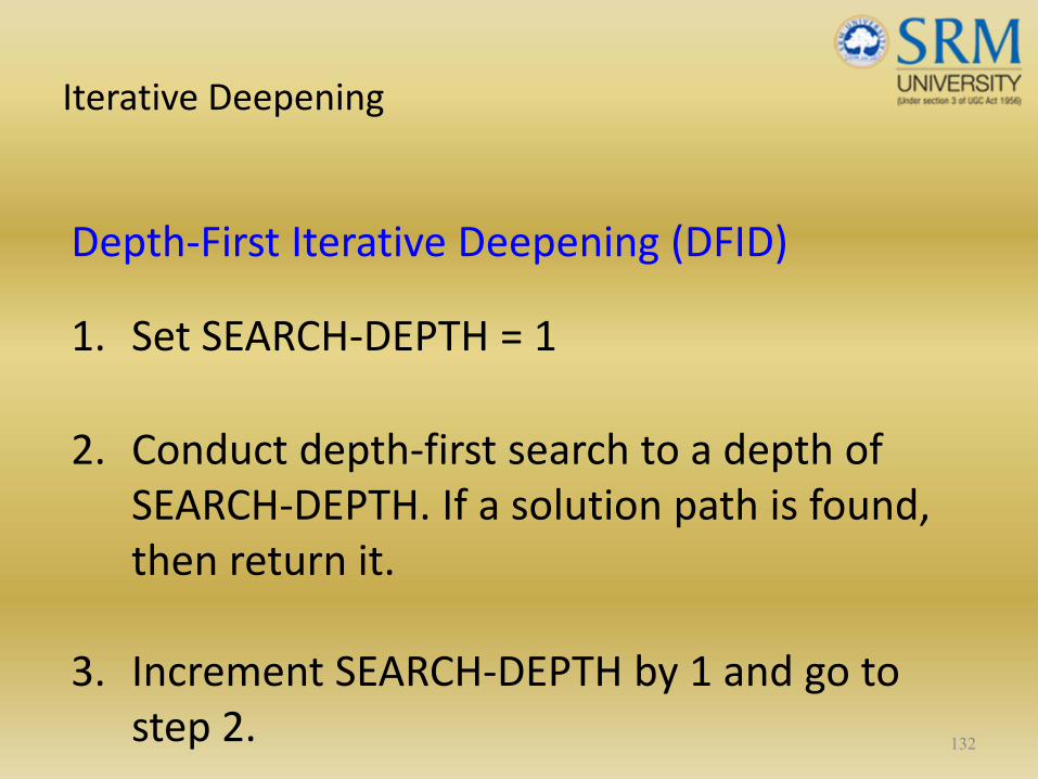
Depth‐First Iterative Deepening (DFID)
1. Set SEARCH‐DEPTH = 1
2. Conduct depth‐first search to a depth of SEARCH‐DEPTH. If a solution path is found, then return it.
3. Increment SEARCH‐DEPTH by 1 and go to step 2. 132
Iterative Deepening
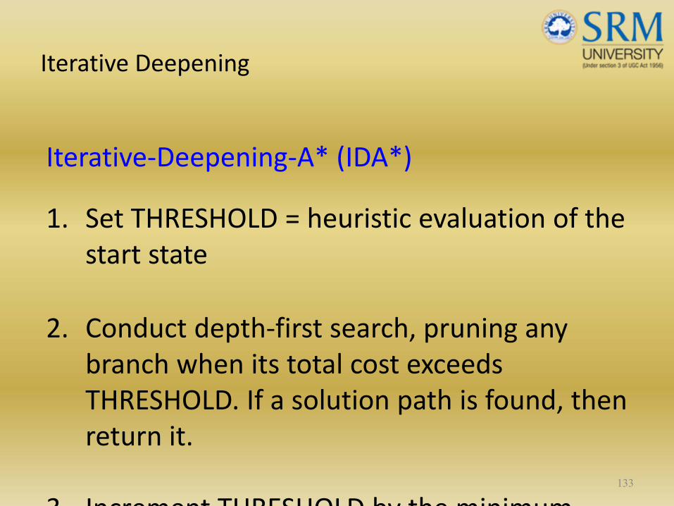
Iterative‐Deepening‐A* (IDA*)
1. Set THRESHOLD = heuristic evaluation of the start state
2. Conduct depth‐first search, pruning any branch when its total cost exceeds THRESHOLD. If a solution path is found, then return it.
3 Increment THRESHOLD by the minimum133

Iterative Deepening
• Is the process wasteful?
134
Homework
Presentations– Specific games: Chess – State of the Art
Exercises 1‐7, 9 (Chapter 12)
135

136
Solving problems by searching
Chapter 3
Outline
• Problem‐solving agents
• Problem types
• Problem formulation
• Example problems
• Basic search algorithms
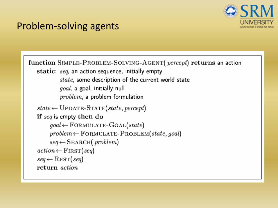
Problem‐solving agents

Example: Romania
• On holiday in Romania; currently in Arad.• Flight leaves tomorrow from Bucharest•• Formulate goal:
– be in Bucharest–
• Formulate problem:– states: various cities– actions: drive between cities–
• Find solution:– sequence of cities, e.g., Arad, Sibiu, Fagaras, Bucharest–

Example: Romania

Problem types
• Deterministic, fully observable single‐state problem– Agent knows exactly which state it will be in; solution is a sequence–
• Non‐observable sensorless problem (conformant problem)– Agent may have no idea where it is; solution is a sequence–
• Nondeterministic and/or partially observable contingency problem– percepts provide new information about current state– often interleave} search, execution–
• Unknown state space exploration problem
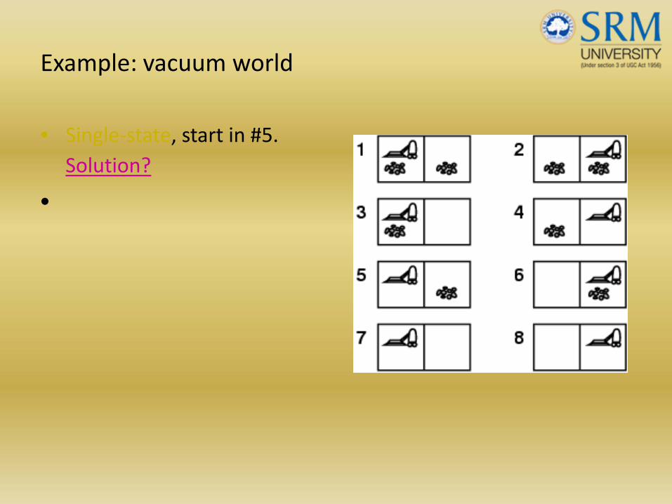
Example: vacuum world
• Single‐state, start in #5. Solution?
•

Example: vacuum world
• Single‐state, start in #5. Solution? [Right, Suck]
•
• Sensorless, start in {1,2,3,4,5,6,7,8} e.g., Right goes to {2,4,6,8} Solution?
•

Example: vacuum world
• Sensorless, start in {1,2,3,4,5,6,7,8} e.g., Right goes to {2,4,6,8} Solution?[Right,Suck,Left,Suck]
•
• Contingency– Nondeterministic: Suckmay
dirty a clean carpet– Partially observable: location, dirt at current location.– Percept: [L, Clean], i.e., start in #5 or #7
Solution?

Example: vacuum world
• Sensorless, start in {1,2,3,4,5,6,7,8} e.g., Right goes to {2,4,6,8} Solution?[Right,Suck,Left,Suck]
•
• Contingency– Nondeterministic: Suckmay
dirty a clean carpet– Partially observable: location, dirt at current location.– Percept: [L, Clean], i.e., start in #5 or #7
Solution? [Right, if dirt then Suck]
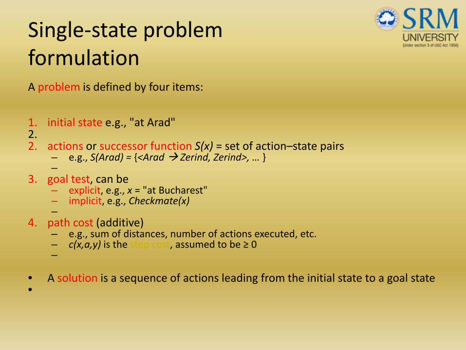
Single‐state problem formulationA problem is defined by four items:
1. initial state e.g., "at Arad"2.2. actions or successor function S(x) = set of action–state pairs
– e.g., S(Arad) = {<Arad Zerind, Zerind>, … }–
3. goal test, can be– explicit, e.g., x = "at Bucharest"– implicit, e.g., Checkmate(x)–
4. path cost (additive)– e.g., sum of distances, number of actions executed, etc.– c(x,a,y) is the step cost, assumed to be ≥ 0–
• A solution is a sequence of actions leading from the initial state to a goal state•

Selecting a state space
• Real world is absurdly complex state space must be abstracted for problem solving
• (Abstract) state = set of real states•• (Abstract) action = complex combination of real actions
– e.g., "Arad Zerind" represents a complex set of possible routes, detours, rest stops, etc.
• For guaranteed realizability, any real state "in Arad“ must get to some real state "in Zerind"
•• (Abstract) solution =
– set of real paths that are solutions in the real world–
• Each abstract action should be "easier" than the original problem•
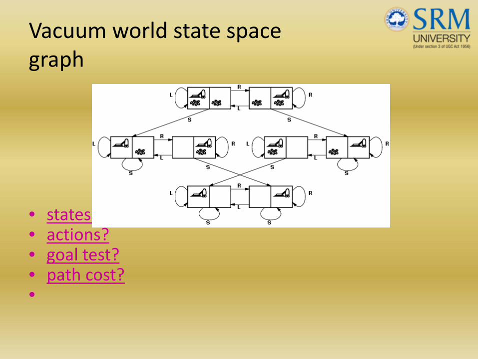
Vacuum world state space graph
• states?• actions?• goal test?• path cost?•
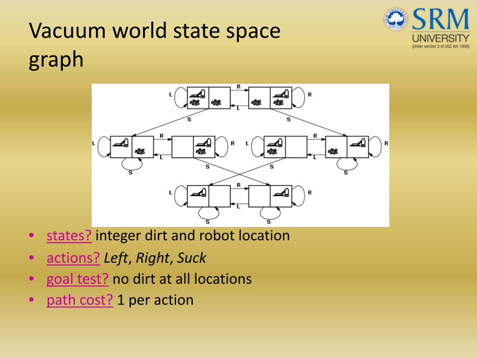
Vacuum world state space graph
• states? integer dirt and robot location• actions? Left, Right, Suck• goal test? no dirt at all locations• path cost? 1 per action

Example: The 8‐puzzle
• states?
• actions?
• goal test?
• path cost?
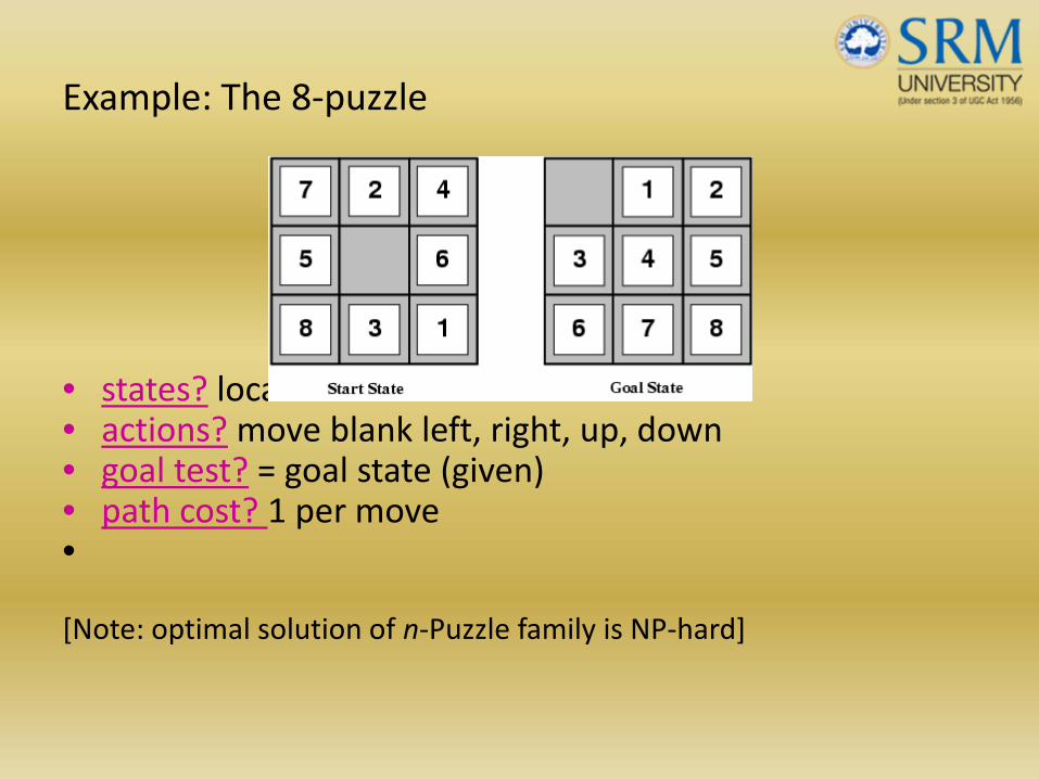
Example: The 8‐puzzle
• states? locations of tiles • actions? move blank left, right, up, down • goal test? = goal state (given)• path cost? 1 per move•
[Note: optimal solution of n‐Puzzle family is NP‐hard]
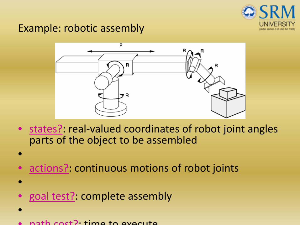
Example: robotic assembly
• states?: real‐valued coordinates of robot joint angles parts of the object to be assembled
•• actions?: continuous motions of robot joints•• goal test?: complete assembly•• path cost?: time to execute
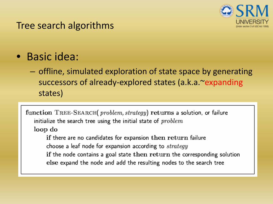
Tree search algorithms
• Basic idea:– offline, simulated exploration of state space by generating successors of already‐explored states (a.k.a.~expandingstates)
–

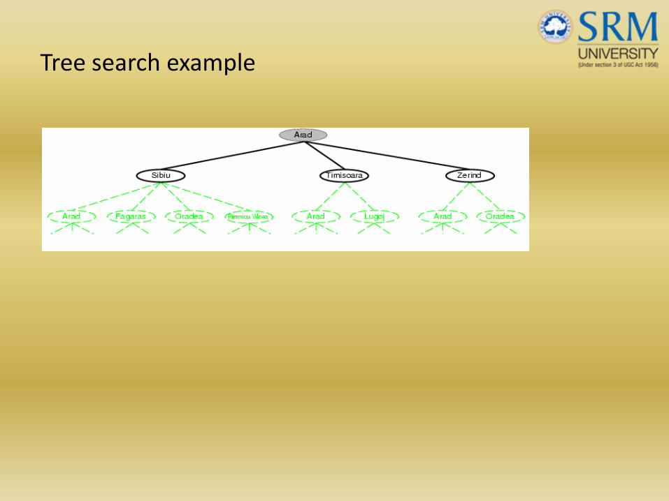
Tree search example
Tree search example
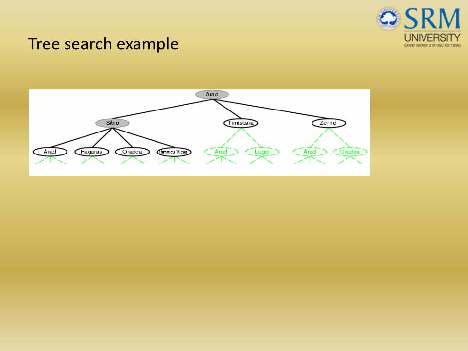
Tree search example
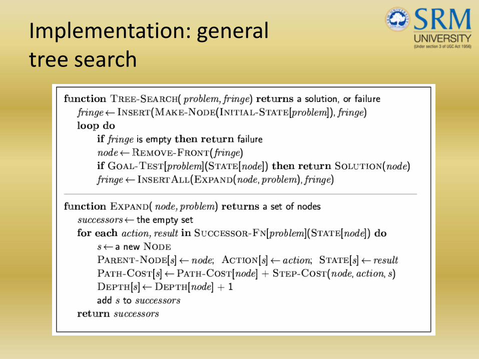
Implementation: general tree search
Implementation: states vs. nodes
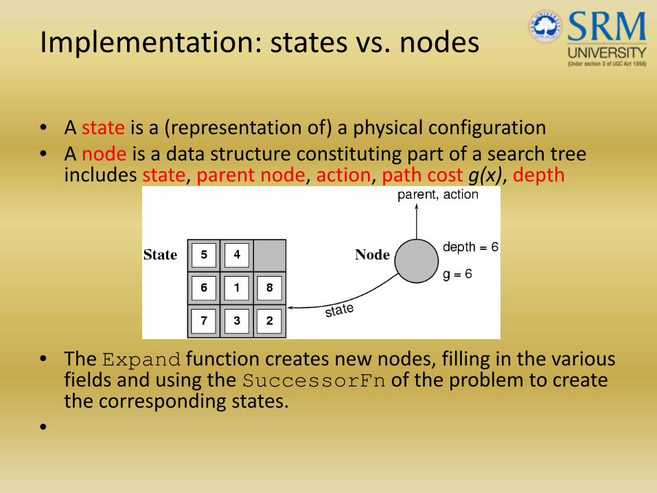
• A state is a (representation of) a physical configuration• A node is a data structure constituting part of a search tree
includes state, parent node, action, path cost g(x), depth
• The Expand function creates new nodes, filling in the various fields and using the SuccessorFn of the problem to create the corresponding states.
•
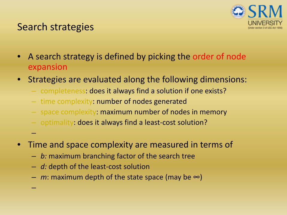
Search strategies
• A search strategy is defined by picking the order of node expansion
• Strategies are evaluated along the following dimensions:– completeness: does it always find a solution if one exists?– time complexity: number of nodes generated– space complexity: maximum number of nodes in memory– optimality: does it always find a least‐cost solution?–
• Time and space complexity are measured in terms of – b:maximum branching factor of the search tree– d: depth of the least‐cost solution– m: maximum depth of the state space (may be ∞)–
Uninformed search strategies
• Uninformed search strategies use only the information available in the problem definition
•• Breadth‐first search
•• Uniform‐cost search
•• Depth‐first search
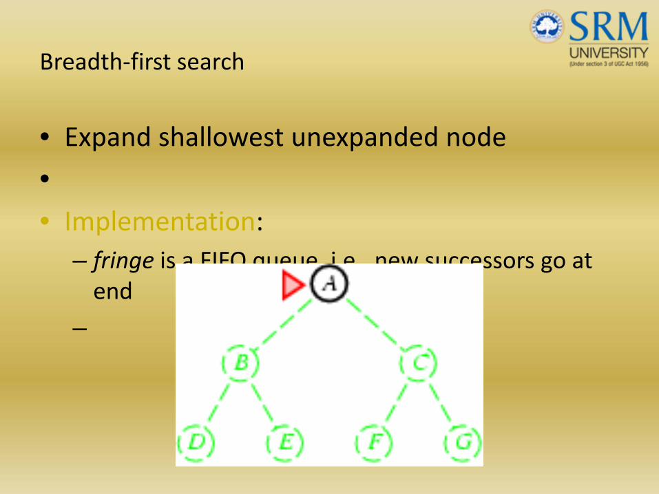
Breadth‐first search
• Expand shallowest unexpanded node
•• Implementation:
– fringe is a FIFO queue, i.e., new successors go at end
–

Breadth‐first search
• Expand shallowest unexpanded node
•• Implementation:
– fringe is a FIFO queue, i.e., new successors go at end
–
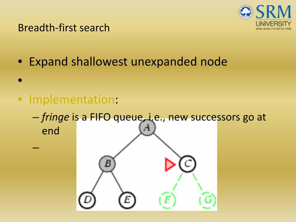
Breadth‐first search
• Expand shallowest unexpanded node
•• Implementation:
– fringe is a FIFO queue, i.e., new successors go at end
–
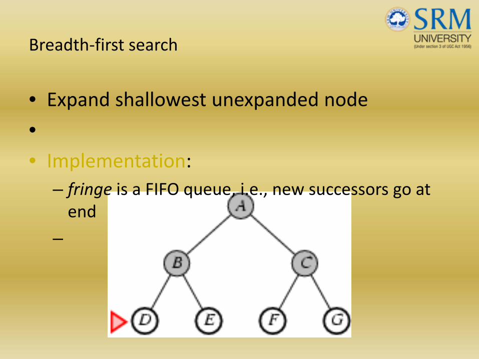
Breadth‐first search
• Expand shallowest unexpanded node
•• Implementation:
– fringe is a FIFO queue, i.e., new successors go at end
–
Properties of breadth‐first search• Complete? Yes (if b is finite)•• Time? 1+b+b2+b3+… +bd + b(bd‐1) = O(bd+1)•• Space? O(bd+1) (keeps every node in memory)•• Optimal? Yes (if cost = 1 per step)•
• Space is the bigger problem (more than time)•

Uniform‐cost search
• Expand least‐cost unexpanded node•• Implementation:
– fringe = queue ordered by path cost–
• Equivalent to breadth‐first if step costs all equal•• Complete? Yes, if step cost ≥ ε•• Time? # of nodes with g ≤ cost of optimal solution, O(bceiling(C*/
ε)) where C* is the cost of the optimal solution• Space? # of nodes with g ≤ cost of optimal solution,
O(bceiling(C*/ ε))•
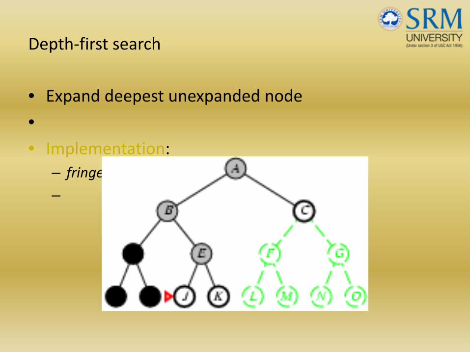
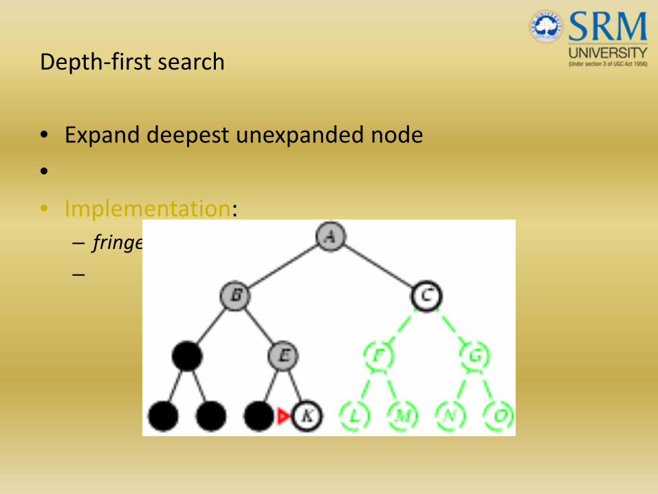
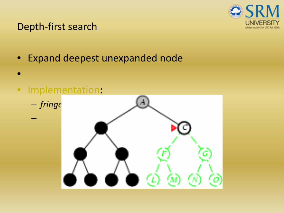
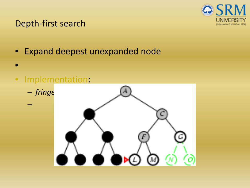
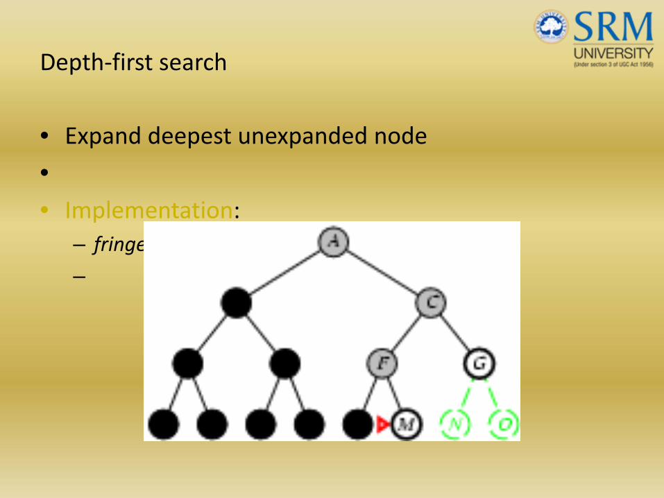
Depth‐first search
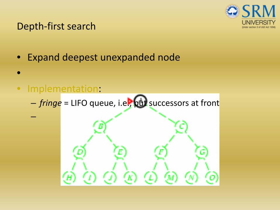
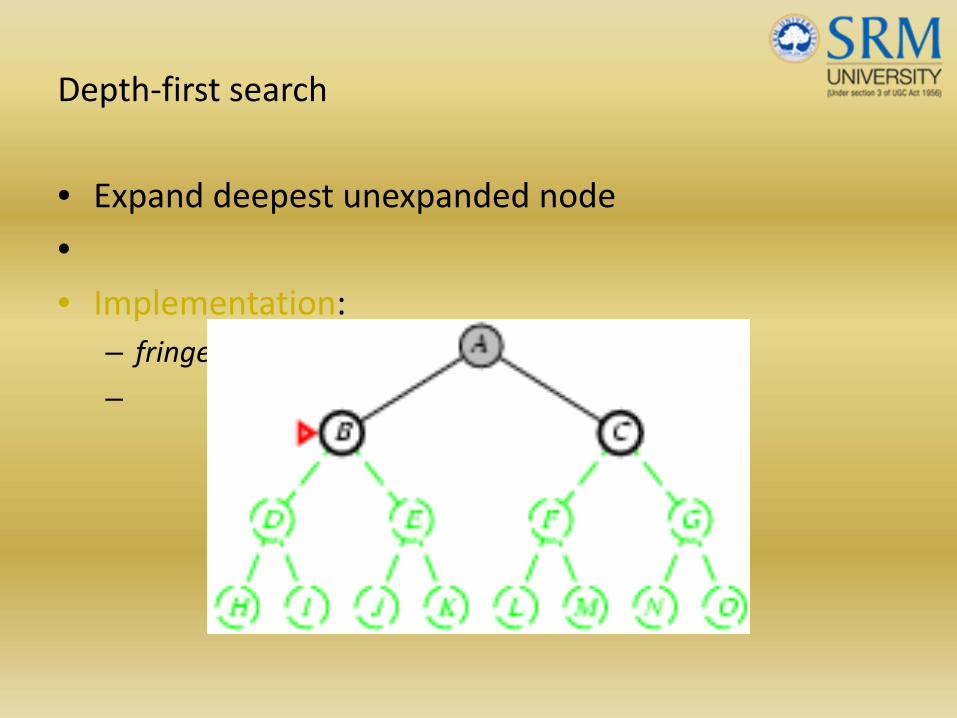
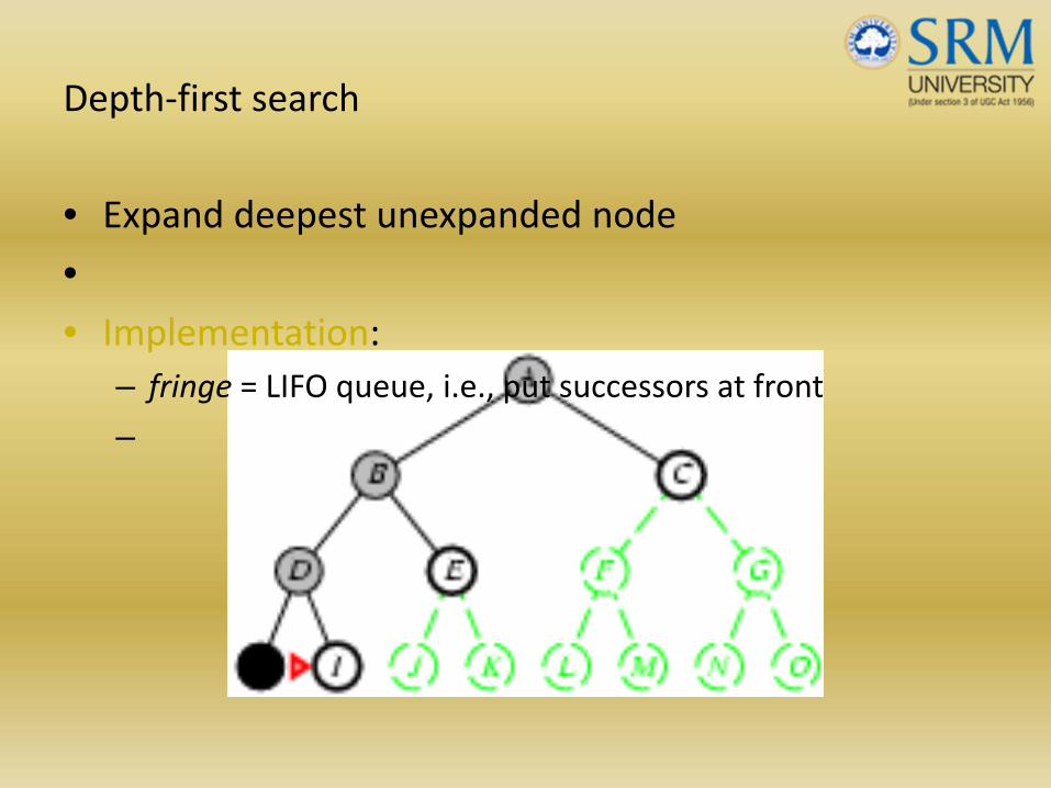
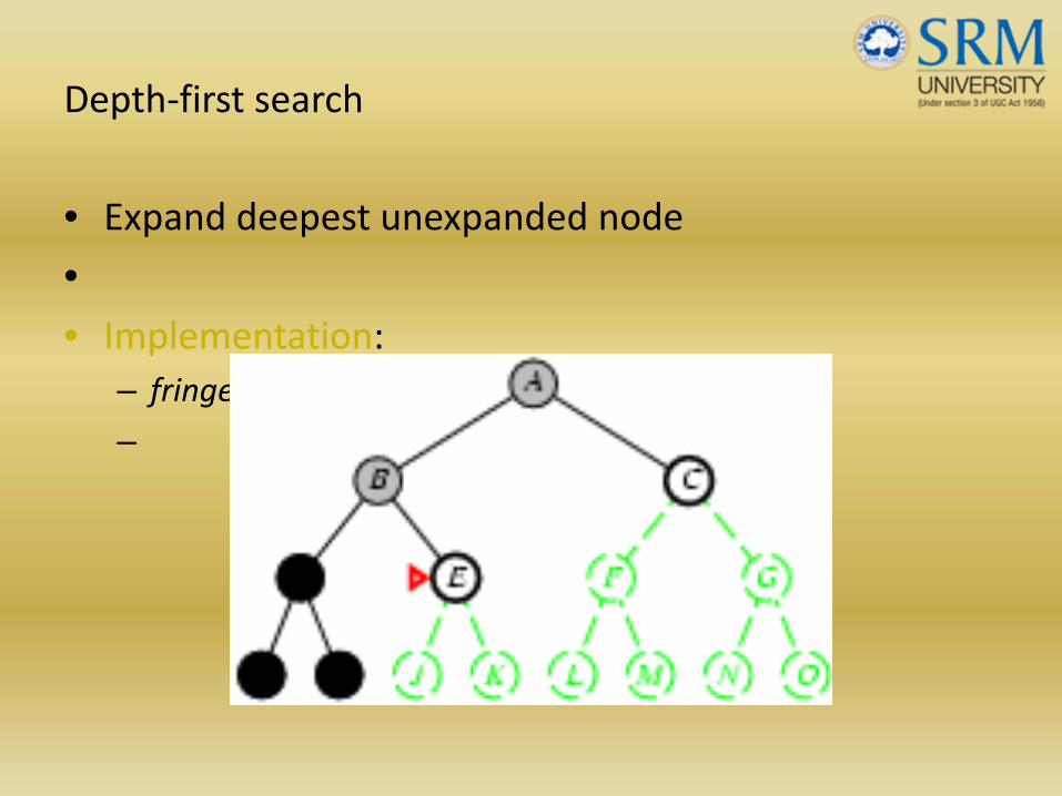
• Expand deepest unexpanded node
•• Implementation:
– fringe = LIFO queue, i.e., put successors at front
–
Depth‐first search
• Expand deepest unexpanded node
•• Implementation:
– fringe = LIFO queue, i.e., put successors at front
–

Depth‐first search
• Expand deepest unexpanded node
•• Implementation:
– fringe = LIFO queue, i.e., put successors at front
–

Depth‐first search
• Expand deepest unexpanded node
•• Implementation:
– fringe = LIFO queue, i.e., put successors at front
–
Depth‐first search
• Expand deepest unexpanded node
•• Implementation:
– fringe = LIFO queue, i.e., put successors at front
–
Depth‐first search
• Expand deepest unexpanded node
•• Implementation:
– fringe = LIFO queue, i.e., put successors at front
–
Depth‐first search
• Expand deepest unexpanded node
•• Implementation:
– fringe = LIFO queue, i.e., put successors at front
–
Depth‐first search
• Expand deepest unexpanded node
•• Implementation:
– fringe = LIFO queue, i.e., put successors at front
–
Depth‐first search
• Expand deepest unexpanded node
•• Implementation:
– fringe = LIFO queue, i.e., put successors at front
–

Depth‐first search
• Expand deepest unexpanded node
•• Implementation:
– fringe = LIFO queue, i.e., put successors at front
–
Depth‐first search
• Expand deepest unexpanded node
•• Implementation:
– fringe = LIFO queue, i.e., put successors at front
–
Depth‐first search
• Expand deepest unexpanded node
•• Implementation:
– fringe = LIFO queue, i.e., put successors at front
–
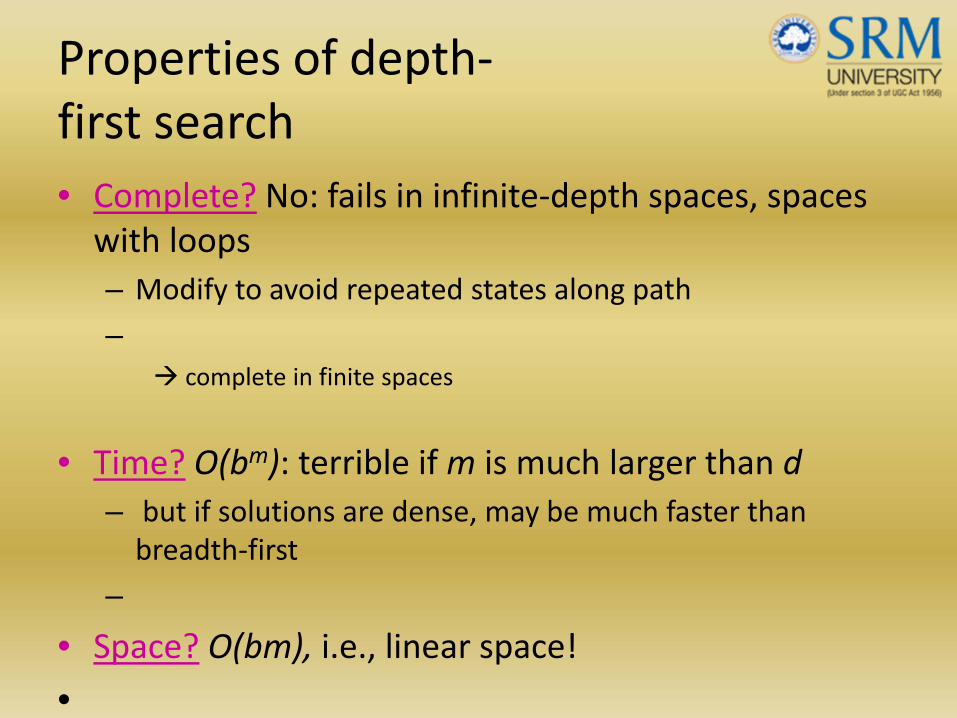
Properties of depth‐first search• Complete? No: fails in infinite‐depth spaces, spaces with loops– Modify to avoid repeated states along path
–complete in finite spaces
• Time? O(bm): terrible if m is much larger than d– but if solutions are dense, may be much faster than breadth‐first
–• Space? O(bm), i.e., linear space!
•
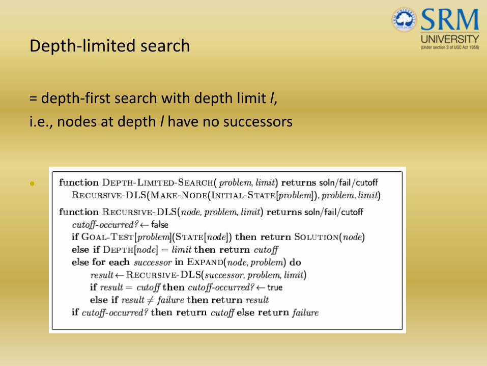
Depth‐limited search
= depth‐first search with depth limit l,
i.e., nodes at depth l have no successors
• Recursive implementation:
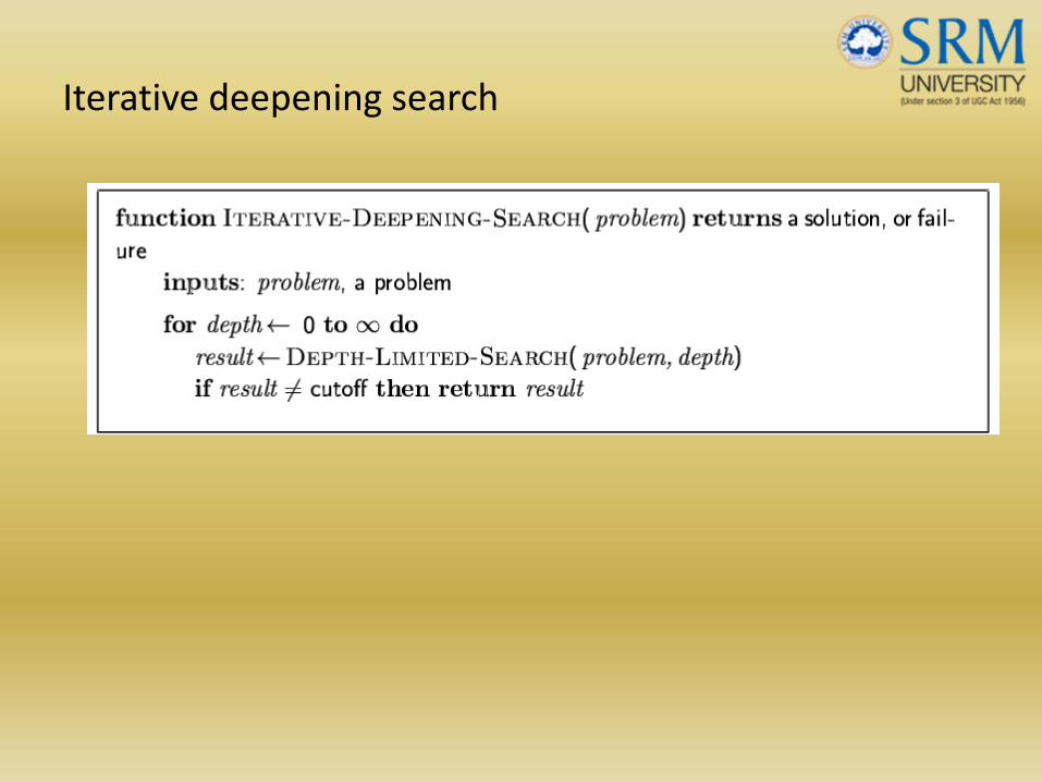
Iterative deepening search

Iterative deepening search l =0
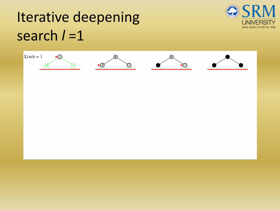
Iterative deepening search l =1
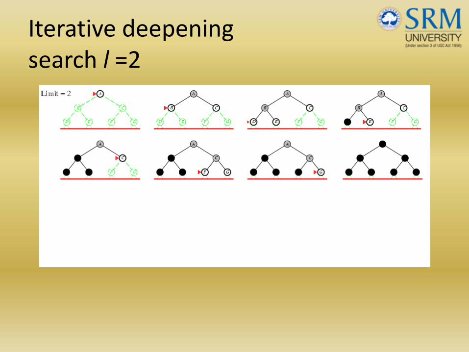
Iterative deepening search l =2
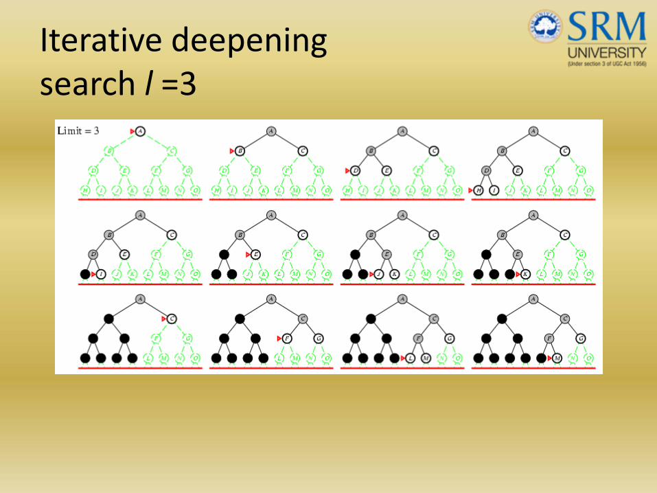
Iterative deepening search l =3
Iterative deepening search
• Number of nodes generated in a depth‐limited search to depth d with branching factor b:
NDLS = b0 + b1 + b2 + … + bd-2 + bd-1 + bd
• Number of nodes generated in an iterative deepening search to depth d with branching factor b: NIDS = (d+1)b0 + d b^1 + (d‐1)b^2 + … + 3bd‐2 +2bd‐1 + 1bd
• For b = 10, d = 5,•
– NDLS = 1 + 10 + 100 + 1,000 + 10,000 + 100,000 = 111,111–– NIDS = 6 + 50 + 400 + 3,000 + 20,000 + 100,000 = 123,456–
• Overhead = (123 456 111 111)/111 111 = 11%
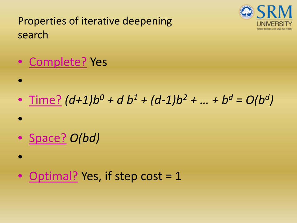
Properties of iterative deepening search
• Complete? Yes
•• Time? (d+1)b0 + d b1 + (d‐1)b2 + … + bd = O(bd)
•• Space? O(bd)
•• Optimal? Yes, if step cost = 1
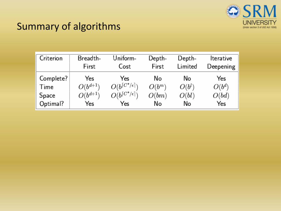
Summary of algorithms
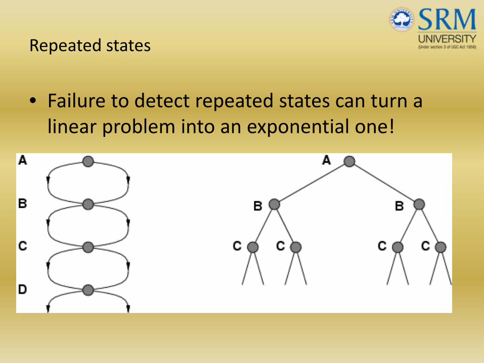
Repeated states
• Failure to detect repeated states can turn a linear problem into an exponential one!
•
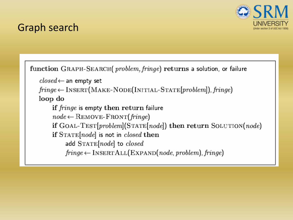
Graph search
Summary
• Problem formulation usually requires abstracting away real‐world details to define a state space that can feasibly be explored
•
• Variety of uninformed search strategies
•
• Iterative deepening search uses only linear space and not much more time than other uninformed algorithms
•


![CS 294-5: Statistical Natural Language Processing · PDF fileAll CS188 materials are available at .] Linear Classifiers. ... Problems with the ... other training examples are ignorable](https://static.fdocuments.in/doc/165x107/5aabcd007f8b9a59658c4cff/cs-294-5-statistical-natural-language-processing-cs188-materials-are-available.jpg)


