Probability - UC3Mhalweb.uc3m.es/esp/Personal/personas/mwiper/docencia/English/PhD... ·...

Probability

Chance is a part of our everyday lives. Everyday we make judgements basedon probability:

• There is a 90% chance Real Madrid will win tomorrow.

• There is a 1/6 chance that a dice toss will be a 3.

Probability Theory was developed from the study of games of chance by Fermatand Pascal and is the mathematical study of randomness. This theory dealswith the possible outcomes of an event and was put onto a firm mathematicalbasis by Kolmogorov.

Statistics and Probability

The Kolmogorov axioms

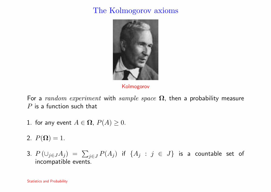
Kolmogorov

For a random experiment with sample space Ω, then a probability measureP is a function such that

1. for any event A ∈ Ω, P (A) ≥ 0.

2. P (Ω) = 1.

3. P (∪j∈JAj) =∑

j∈J P (Aj) if Aj : j ∈ J is a countable set ofincompatible events.


Set theory

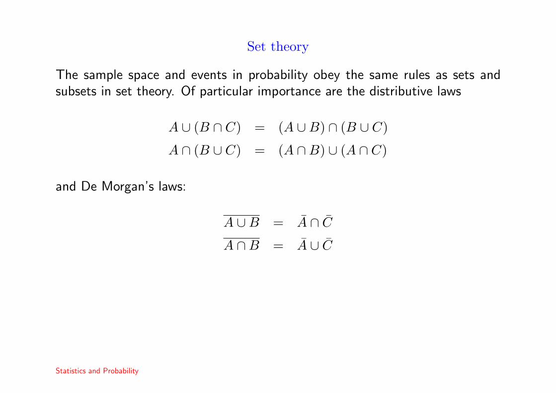
The sample space and events in probability obey the same rules as sets andsubsets in set theory. Of particular importance are the distributive laws

A ∪ (B ∩ C) = (A ∪B) ∩ (B ∪ C)

A ∩ (B ∪ C) = (A ∩B) ∪ (A ∩ C)

and De Morgan’s laws:

A ∪B = A ∩ C

A ∩B = A ∪ C


Laws of probability

The basic laws of probability can be derived directly from set theory and theKolmogorov axioms. For example, for any two events A and B, we have theaddition law,

P (A ∪B) = P (A) + P (B)− P (A ∩B).

Laws of probability

The basic laws of probability can be derived directly from set theory and theKolmogorov axioms. For example, for any two events A and B, we have theaddition law,

P (A ∪B) = P (A) + P (B)− P (A ∩B).

Proof

A = A ∩ Ω

= A ∩ (B ∪ B)

= (A ∩B) ∪ (A ∩ B) by the second distributive law, so

P (A) = P (A ∩B) + P (A ∩ B) and similarly for B.


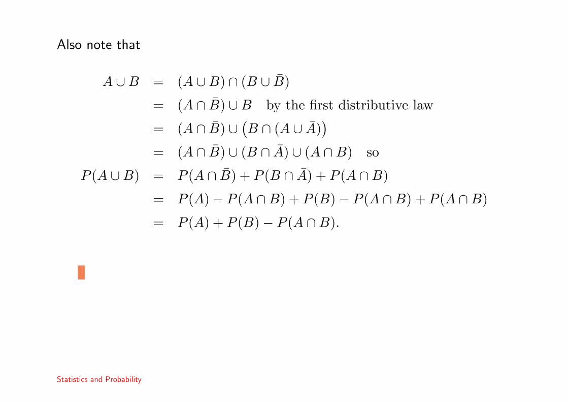
Also note that

A ∪B = (A ∪B) ∩ (B ∪ B)

= (A ∩ B) ∪B by the first distributive law

= (A ∩ B) ∪(B ∩ (A ∪ A)

)= (A ∩ B) ∪ (B ∩ A) ∪ (A ∩B) so

P (A ∪B) = P (A ∩ B) + P (B ∩ A) + P (A ∩B)

= P (A)− P (A ∩B) + P (B)− P (A ∩B) + P (A ∩B)

= P (A) + P (B)− P (A ∩B).


Partitions

The previous example is easily extended when we have a sequence of events,A1, A2, . . . , An, that form a partition, that is

n⋃i=1

Ai = Ω, Ai ∩Aj = φ for all i 6= j.

In this case,

P (∪ni=1Ai) =

n∑i=1

P (Ai)−n∑

j>i=1

P (Ai ∩Aj) +n∑

k>j>i=1

P (Ai ∩Aj ∩Ak) + . . .

+(−1)nP (A1 ∩A2 ∩ . . . ∩An).


Interpretations of probability

The Kolmogorov axioms provide a mathematical basis for probability but don’tprovide for a real life interpretation. Various ways of interpreting probability inreal life situations have been proposed.

• Frequentist probability.

• The classical interpretation.

• Subjective probability.

• Other approaches; logical probability and propensities.


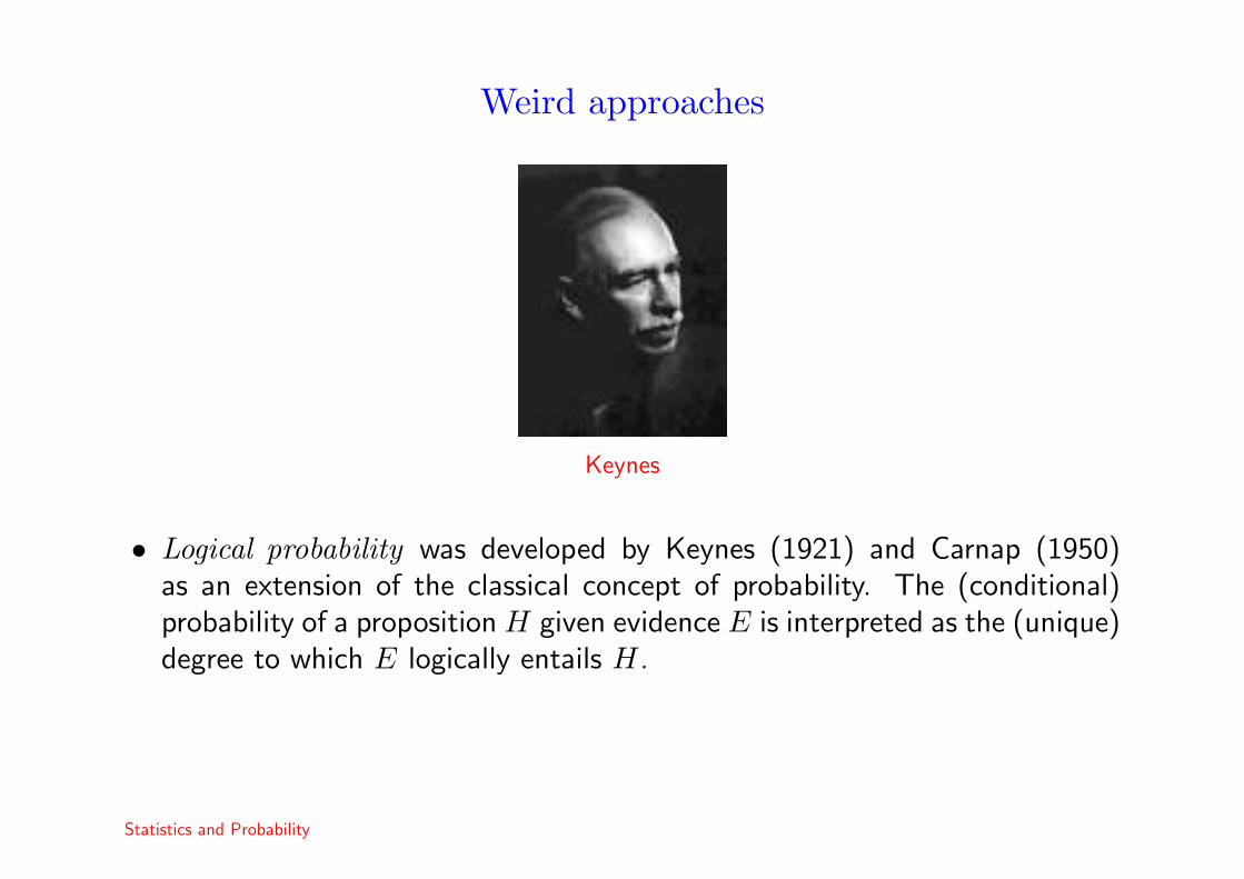
Weird approaches

Keynes

• Logical probability was developed by Keynes (1921) and Carnap (1950)as an extension of the classical concept of probability. The (conditional)probability of a proposition H given evidence E is interpreted as the (unique)degree to which E logically entails H.


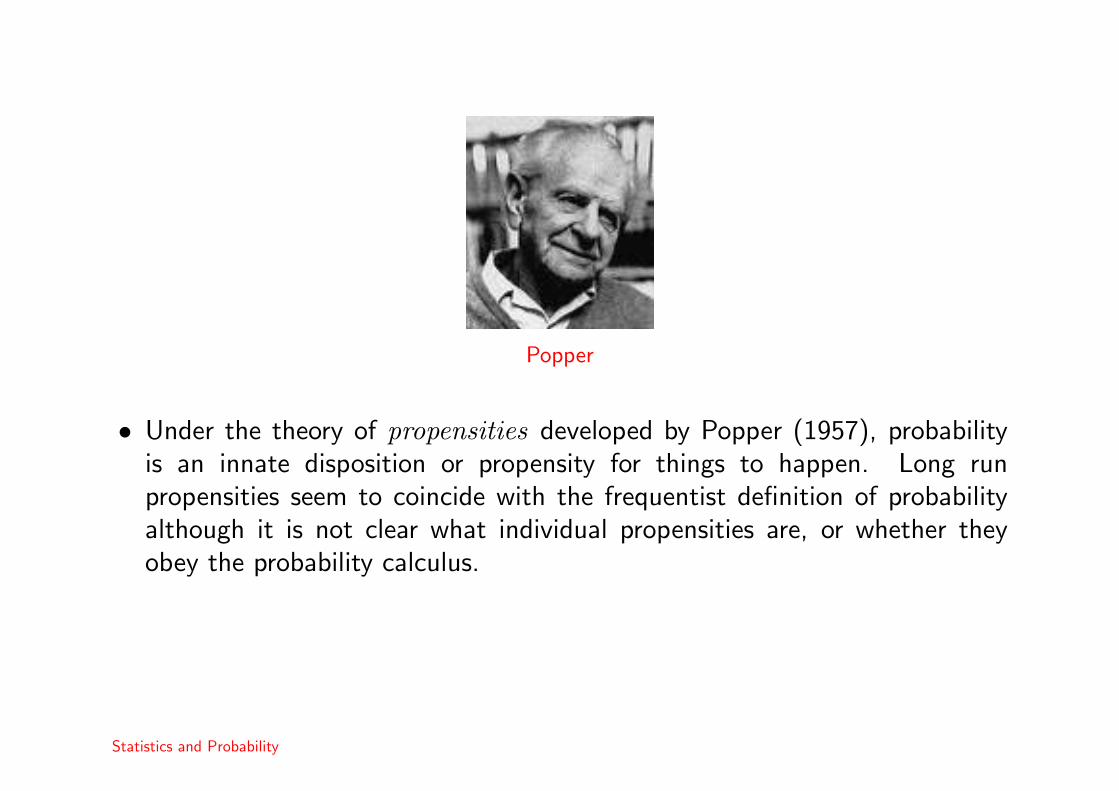
Popper

• Under the theory of propensities developed by Popper (1957), probabilityis an innate disposition or propensity for things to happen. Long runpropensities seem to coincide with the frequentist definition of probabilityalthough it is not clear what individual propensities are, or whether theyobey the probability calculus.


Frequentist probability

Venn Von Mises

The idea comes from Venn (1876) and von Mises (1919).

Given a repeatable experiment, the probability of an event is defined to be thelimit of the proportion of times that the event will occur when the number ofrepetitions of the experiment tends to infinity.

This is a restricted definition of probability. It is impossible to assignprobabilities in non repeatable experiments.


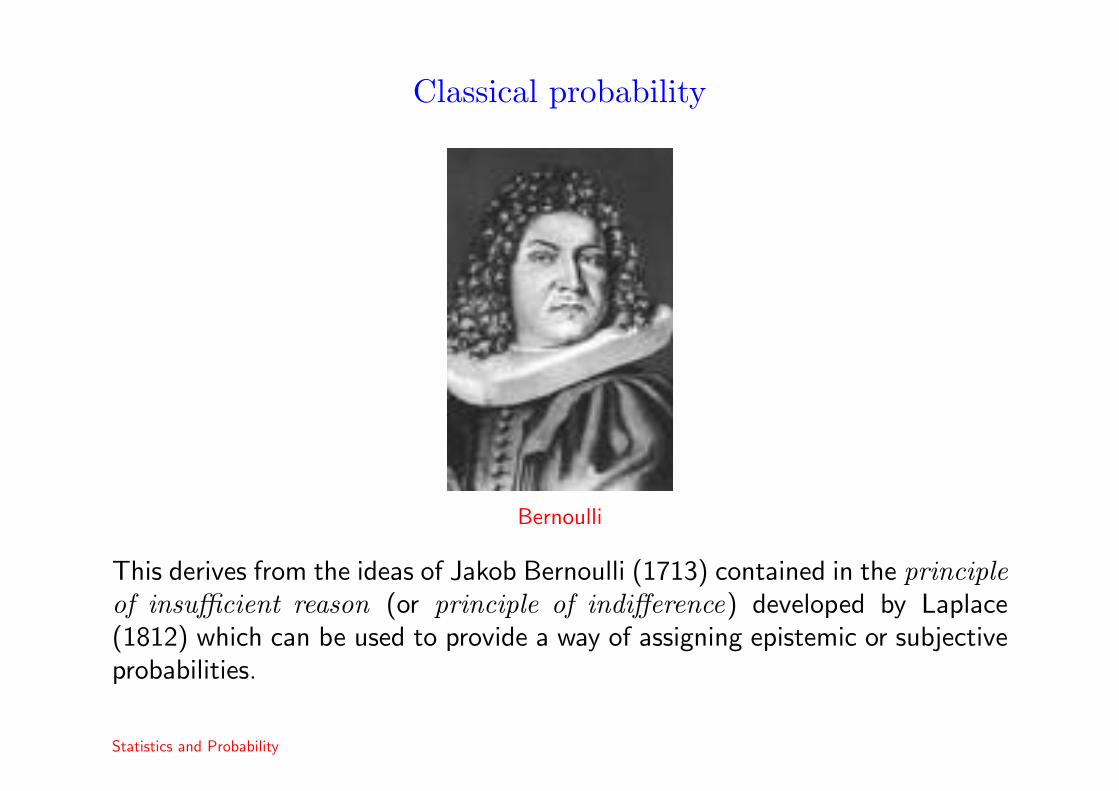
Classical probability

Bernoulli

This derives from the ideas of Jakob Bernoulli (1713) contained in the principleof insufficient reason (or principle of indifference) developed by Laplace(1812) which can be used to provide a way of assigning epistemic or subjectiveprobabilities.


The principle of insufficient reason

If we are ignorant of the ways an event can occur (and therefore have noreason to believe that one way will occur preferentially compared to another),the event will occur equally likely in any way.

Thus the probability of an event, S, is the coefficient between the number offavourable cases and the total number of possible cases, that is

P (S) =|S||Ω|

.


Calculating classical probabilities

The calculation of classical probabilities involves being able to count thenumber of possible and the number of favourable results in the sample space.In order to do this, we often use variations, permutations and combinations.

Variations

Suppose we wish to draw n cards from a pack of size N without replacement,then the number of possible results is

V nN = N × (N − 1)× (N − n + 1) =

N !(N − n)!

.

Note that one variation is different from another if the order in which the cardsare drawn is different.

We can also consider the case of drawing cards with replacement. In this case,the number of possible results is V Rn

N = Nn.


Example: The birthday problem

What is the probability that among n students in a classroom, at least twowill have the same birthday?

Example: The birthday problem

What is the probability that among n students in a classroom, at least twowill have the same birthday?

To simplify the problem, assume there are 365 days in a year and that theprobability of being born is the same for every day.

Let Sn be the event that at least 2 people have the same birthday.

P (Sn) = 1− P (Sn)

= 1− # elementary events where nobody has the same birthday# elementary events

= 1− # elementary events where nobody has the same birthday365n

because the denominator is a variation with repetition.


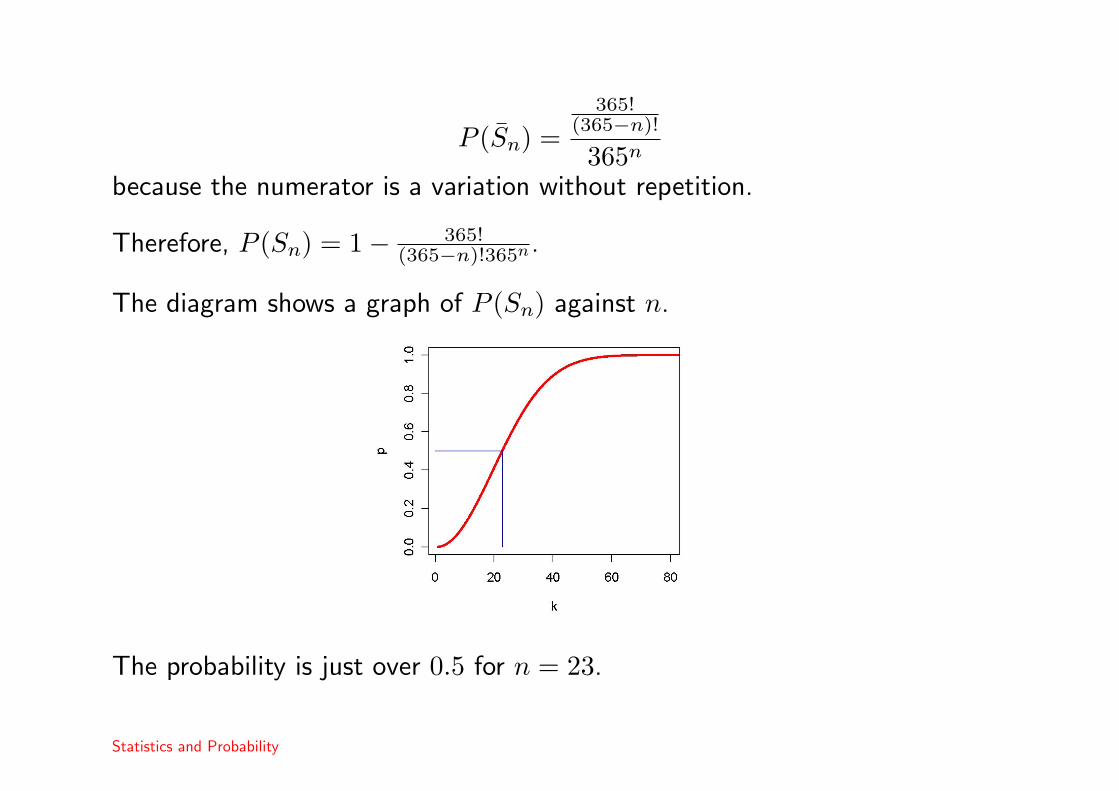
P (Sn) =365!

(365−n)!

365n

because the numerator is a variation without repetition.

Therefore, P (Sn) = 1− 365!(365−n)!365n.

The diagram shows a graph of P (Sn) against n.

The probability is just over 0.5 for n = 23.


Permutations

If we deal all the cards in a pack of size N , then their are PN = N ! possibledeals.

If we assume that the pack contains R1 cards of type one, R2 of suit 2, ... Rk

of type k, then there are

PRR1,...,RkN =

N !R1!× · · · ×Rk!

different deals.Combinations

If we flip a coin N times, how many ways are there that we can get n headsand N − n tails?

CnN =

(Nn

)=

N !n!(N − n)!

.


Example: The probability of winning the Primitiva

In the Primitiva, each player chooses six numbers between one and forty nine.If these numbers all match the six winning numbers, then the player wins thefirst prize. What is the probability of winning?

Example: The probability of winning the Primitiva

In the Primitiva, each player chooses six numbers between one and forty nine.If these numbers all match the six winning numbers, then the player wins thefirst prize. What is the probability of winning?

The game consists of choosing 6 numbers from 49 possible numbers and there

are

(496

)ways of doing this. Only one of these combinations of six numbers

is the winner, so the probability of winning is

1(496

) =1

13983816

or almost 1 in 14 million.


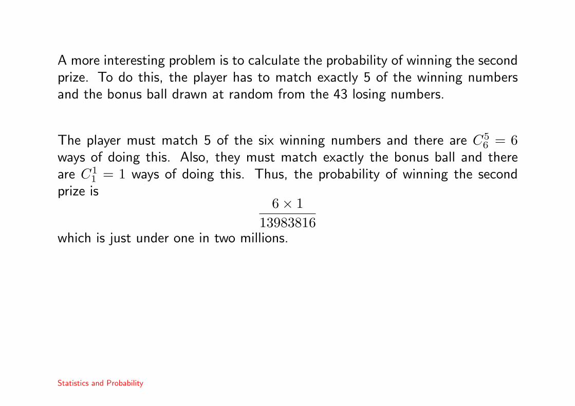
A more interesting problem is to calculate the probability of winning the secondprize. To do this, the player has to match exactly 5 of the winning numbersand the bonus ball drawn at random from the 43 losing numbers.

A more interesting problem is to calculate the probability of winning the secondprize. To do this, the player has to match exactly 5 of the winning numbersand the bonus ball drawn at random from the 43 losing numbers.

The player must match 5 of the six winning numbers and there are C56 = 6

ways of doing this. Also, they must match exactly the bonus ball and thereare C1

1 = 1 ways of doing this. Thus, the probability of winning the secondprize is

6× 113983816

which is just under one in two millions.


Subjective probability

Ramsey

A different approach uses the concept of ones own probability as a subjectivemeasure of ones own uncertainty about the occurrence of an event. Thus,we may all have different probabilities for the same event because we all havedifferent experience and knowledge. This approach is more general than theother methods as we can now define probabilities for unrepeatable experiments.Subjective probability is studied in detail in Bayesian Statistics.


Conditional probability and independence

The probability of an event B conditional on an event A is defined as

P (B|A) =P (A ∩B)

P (A).

This can be interpreted as the probability of B given that A occurs.

Two events A and B are called independent if P (A ∩ B) = P (A)P (B) orequivalently if P (B|A) = P (B) or P (A|B) = P (A).


The multiplication law

A restatement of the conditional probability formula is the multiplication law

P (A ∩B) = P (B|A)P (A).

Example 12What is the probability of getting two cups in two draws from a Spanish packof cards?

Write Ci for the event that draw i is a cup for i = 1, 2. Enumerating allthe draws with two cups is not entirely trivial. However, the conditionalprobabilities are easy to calculate:

P (C1 ∩ C2) = P (C2|C1)P (C1) =939× 10

40=

352

.

The multiplication law can be extended to more than two events. For example,

P (A ∩B ∩ C) = P (C|A,B)P (B|A)P (A).


The birthday problem revisited

We can also solve the birthday problem using conditional probability. Let bi bethe birthday of student i, for i = 1, . . . , n. Then it is easiest to calculate theprobability that all birthdays are distinct

P (b1 6= b2 6= . . . 6= bn) = P (bn /∈ b1, . . . , bn−1|b1 6= b2 6= . . . bn−1)×P (bn−1 /∈ b1, . . . , bn−2|b1 6= b2 6= . . . bn−2)× · · ·×P (b3 /∈ b1, b2|b1 6= b2)P (b1 6= b2)


Now clearly,

P (b1 6= b2) =364365

, P (b3 /∈ b1, b2|b1 6= b2) =363365

and similarly

P (bi /∈ b1, . . . , bi−1|b1 6= b2 6= . . . bi−1) =366− i

365

for i = 3, . . . , n.

Thus, the probability that at least two students have the same birthday is, forn < 365,

1− 364365

× · · · × 366− n

365=

365!365n(365− n)!

.


The law of total probability

The simplest version of this rule is the following.

Theorem 3For any two events A and B, then

P (B) = P (B|A)P (A) + P (B|A)P (A).

We can also extend the law to the case where A1, . . . , An form a partition. Inthis case, we have

P (B) =n∑

i=1

P (B|Ai)P (Ai).


Bayes theorem

Theorem 4For any two events A and B, then

P (A|B) =P (B|A)P (A)

P (B).

Supposing that A1, . . . , An form a partition, using the law of total probability,we can write Bayes theorem as

P (Aj|B) =P (B|Aj)P (Aj)∑ni=1 P (B|Ai)P (Ai)

for j = 1, . . . , n.


The Monty Hall problem

Example 13The following statement of the problem was given in a column by Marilyn vosSavant in a column in Parade magazine in 1990.

Suppose you’re on a game show, and you’re given the choice of three doors:Behind one door is a car; behind the others, goats. You pick a door, say No.1, and the host, who knows what’s behind the doors, opens another door,say No. 3, which has a goat. He then says to you, “Do you want to pickdoor No. 2?” Is it to your advantage to switch your choice?


Simulating the game

Have a look at the following web page.

http://www.stat.sc.edu/~west/javahtml/LetsMakeaDeal.html

Simulating the game

Have a look at the following web page.

http://www.stat.sc.edu/~west/javahtml/LetsMakeaDeal.html

Using Bayes theorem

http://en.wikipedia.org/wiki/Monty_Hall_problem


Random variables

A random variable generalizes the idea of probabilities for events. Formally, arandom variable, X simply assigns a numerical value, xi to each event, Ai,in the sample space, Ω. For mathematicians, we can write X in terms of amapping, X : Ω → R.

Random variables may be classified according to the values they take as

• discrete

• continuous

• mixed


Discrete variables

Discrete variables are those which take a discrete set range of values, sayx1, x2, . . .. For such variables, we can define the cumulative distributionfunction,

FX(x) = P (X ≤ x) =∑

i,xi≤x

P (X = xi)

where P (X = x) is the probability function or mass function.

For a discrete variable, the mode is defined to be the point, x, with maximumprobability, i.e. such that

P (X = x) < P (X = x)for all x 6= x.


Moments

For any discrete variable, X, we can define the mean of X to be

µX = E[X] =∑

i

xiP (X = xi).

Recalling the frequency definition of probability, we can interpret the mean asthe limiting value of the sample mean from this distribution. Thus, this is ameasure of location.

In general we can define the expectation of any function, g(X) as

E[g(X)] =∑

i

g(xi)P (X = xi).

In particular, the variance is defined as

σ2 = V [X] = E[(X − µX)2

]and the standard deviation is simply σ =

√σ2. This is a measure of spread.


Probability inequalities

For random variables with given mean and variance, it is often possible tobound certain quantities such as the probability that the variable lies within acertain distance of the mean.

An elementary result is Markov’s inequality.

Theorem 5Suppose that X is a non-negative random variable with mean E[X] < ∞.Then for any x > 0,

P (X ≥ x) ≤ E[X]x

.


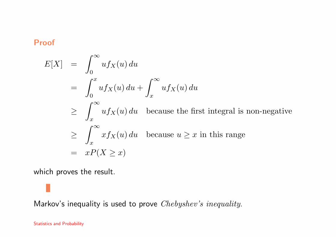
Proof

E[X] =∫ ∞

0

ufX(u) du

=∫ x

0

ufX(u) du +∫ ∞

x

ufX(u) du

≥∫ ∞

x

ufX(u) du because the first integral is non-negative

≥∫ ∞

x

xfX(u) du because u ≥ x in this range

= xP (X ≥ x)

which proves the result.

Markov’s inequality is used to prove Chebyshev’s inequality.


Chebyshev’s inequality

It is interesting to analyze the probability of being close or far away from themean of a distribution. Chebyshev’s inequality provides loose bounds whichare valid for any distribution with finite mean and variance.

Theorem 6For any random variable, X, with finite mean, µ, and variance, σ2, then forany k > 0,

P (|X − µ| ≥ kσ) ≤ 1k2

.

Therefore, for any random variable, X, we have, for example that P (µ− 2σ <X < µ + 2σ) ≥ 3

4.


Proof

P (|X − µ| ≥ kσ) = P((X − µ)2 ≥ k2σ2

)≤

E[(X − µ)2

]k2σ2

by Markov’s inequality

=1k2

Chebyshev’s inequality shows us, for example, that P (µ −√

2σ ≤ X ≤µ +

√2σ) ≥ 0.5 for any variable X.


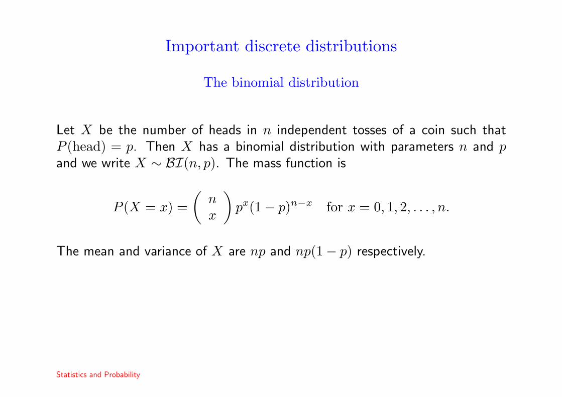
Important discrete distributions

The binomial distribution

Let X be the number of heads in n independent tosses of a coin such thatP (head) = p. Then X has a binomial distribution with parameters n and pand we write X ∼ BI(n, p). The mass function is

P (X = x) =(

nx

)px(1− p)n−x for x = 0, 1, 2, . . . , n.

The mean and variance of X are np and np(1− p) respectively.


An inequality for the binomial distribution

Chebyshev’s inequality is not very tight. For the binomial distribution, a muchstronger result is available.

Theorem 7Let X ∼ BI(n, p). Then

P (|X − np| > nε) ≤ 2e−2nε2.

Proof See Wasserman (2003), Chapter 4.


The geometric distribution

Suppose that Y is defined to be the number of tails observed before the firsthead occurs for the same coin. Then Y has a geometric distribution withparameter p, i.e. Y ∼ GE(p) and

P (Y = y) = p(1− p)y for y = 0, 1, 2, . . .

The mean any variance of X are 1−pp and 1−p

p2 respectively.


The negative binomial distribution

A generalization of the geometric distribution is the negative binomialdistribution. If we define Z to be the number of tails observed beforethe r’th head is observed, then Z ∼ NB(r, p) and

P (Z = z) =(

r + z − 1z

)pr(1− p)z for z = 0, 1, 2, . . .

The mean and variance of X are r1−pp and r1−p

p2 respectively.

The negative binomial distribution reduces to the geometric model for the caser = 1.


The hypergeometric distribution

Suppose that a pack of N cards contains R red cards and that we deal n cardswithout replacement. Let X be the number of red cards dealt. Then X hasa hypergeometric distribution with parameters N,R, n, i.e. X ∼ HG(N,R, n)and

P (X = x) =

(Rx

)(N −Rn− x

)(

Nn

) for x = 0, 1, . . . , n.

Example 14In the Primitiva lottery, a contestant chooses 6 numbers from 1 to 49 and 6numbers are drawn without replacement. The contestant wins the grand prizeif all numbers match. The probability of winning is thus

P (X = x) =

(66

)(430

)(

496

) =6!43!49!

=1

13983816.


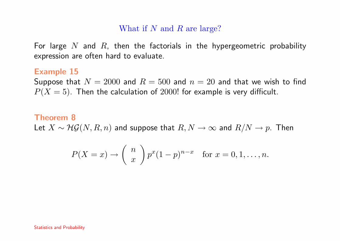
What if N and R are large?

For large N and R, then the factorials in the hypergeometric probabilityexpression are often hard to evaluate.

Example 15Suppose that N = 2000 and R = 500 and n = 20 and that we wish to findP (X = 5). Then the calculation of 2000! for example is very difficult.

What if N and R are large?

For large N and R, then the factorials in the hypergeometric probabilityexpression are often hard to evaluate.

Example 15Suppose that N = 2000 and R = 500 and n = 20 and that we wish to findP (X = 5). Then the calculation of 2000! for example is very difficult.

Theorem 8Let X ∼ HG(N,R, n) and suppose that R,N →∞ and R/N → p. Then

P (X = x) →(

nx

)px(1− p)n−x for x = 0, 1, . . . , n.


Proof

P (X = x) =

(Rx

)(N −Rn− x

)(

Nn

) =

(nx

)(N − nR− x

)(

NR

)=

(nx

)R!(N −R)!(N − n)!

(R− x)!(N −R− n + x)!N !

→(

nx

)Rx(N −R)n−x

Nn→(

nx

)px(1− p)n−x

In the example,p = 500/2000 = 0.25 and using a binomial approximation,

P (X = 5) ≈(

205

)0.2550.7515 = 0.2023. The exact answer, from Matlab

is 0.2024.


The Poisson distribution

Assume that rare events occur on average at a rate λ per hour. Then we canoften assume that the number of rare events X that occur in a time periodof length t has a Poisson distribution with parameter (mean and variance) λt,i.e. X ∼ P(λt). Then

P (X = x) =(λt)xe−λt

x!for x = 0, 1, 2, . . .

The Poisson distribution

Assume that rare events occur on average at a rate λ per hour. Then we canoften assume that the number of rare events X that occur in a time periodof length t has a Poisson distribution with parameter (mean and variance) λt,i.e. X ∼ P(λt). Then

P (X = x) =(λt)xe−λt

x!for x = 0, 1, 2, . . .

Formally, the conditions for a Poisson distribution are

• The numbers of events occurring in non-overlapping intervals areindependent for all intervals.

• The probability that a single event occurs in a sufficiently small interval oflength h is λh + o(h).

• The probability of more than one event in such an interval is o(h).


Continuous variables

Continuous variables are those which can take values in a continuum. For acontinuous variable, X, we can still define the distribution function, FX(x) =P (X ≤ x) but we cannot define a probability function P (X = x). Instead, wehave the density function

fX(x) =dF (x)

dx.

Thus, the distribution function can be derived from the density as FX(x) =∫ x

−∞ fX(u) du. In a similar way, moments of continuous variables can bedefined as integrals,

E[X] =∫ ∞

−∞xfX(x) dx

and the mode is defined to be the point of maximum density.

For a continuous variable, another measure of location is the median, x,defined so that FX(x) = 0.5.


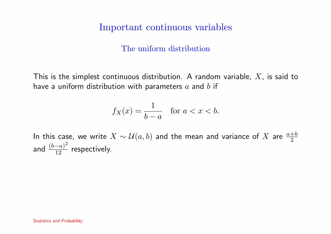
Important continuous variables

The uniform distribution

This is the simplest continuous distribution. A random variable, X, is said tohave a uniform distribution with parameters a and b if

fX(x) =1

b− afor a < x < b.

In this case, we write X ∼ U(a, b) and the mean and variance of X are a+b2

and (b−a)2

12 respectively.


The exponential distribution

Remember that the Poisson distribution models the number of rare eventsoccurring at rate λ in a given time period. In this scenario, consider thedistribution of the time between any two successive events. This is anexponential random variable, Y ∼ E(λ), with density function

fY (y) = λe−λy for y > 0.

The mean and variance of Y are 1λ and 1

λ2 respectively.


The gamma distribution

A distribution related to the exponential distribution is the gamma distribution.If instead of considering the time between 2 random events, we consider thetime between a higher number of random events, then this variable is gammadistributed, that is Y ∼ G(α, λ), with density function

fY (y) =λα

Γ(α)yα−1e−λy for y > 0.

The mean and variance of Y are αλ and α

λ2 respectively.


The normal distribution

This is probably the most important continuous distribution. A randomvariable, X, is said to follow a normal distribution with mean and varianceparameters µ and σ2 if

fX(x) =1

σ√

2πexp

(− 1

2σ2(x− µ)2

)for −∞ < x < ∞.

In this case, we write X ∼ N(µ, σ2

).

• If X is normally distributed, then a + bX is normally distributed. Inparticular, X−µ

σ ∼ N (0, 1).

• P (|X−µ| ≥ σ) = 0.3174, P (|X−µ| ≥ 2σ) = 0.0456, P (|X−µ| ≥ 3σ) =0.0026.

• Any sum of normally distributed variables is also normally distributed.


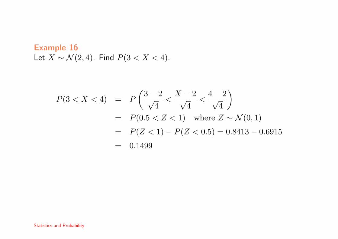
Example 16Let X ∼ N (2, 4). Find P (3 < X < 4).

P (3 < X < 4) = P

(3− 2√

4<

X − 2√4

<4− 2√

4

)= P (0.5 < Z < 1) where Z ∼ N (0, 1)

= P (Z < 1)− P (Z < 0.5) = 0.8413− 0.6915

= 0.1499


The central limit theorem

One of the main reasons for the importance of the normal distribution is thatit can be shown to approximate many real life situations due to the centrallimit theorem.

Theorem 9Given a random sample of size X1, . . . , Xn from some distribution, thenunder certain conditions, the sample mean X = 1

n

∑ni=1 Xi follows a normal

distribution.

Proof See later.

For an illustration of the CLT, see

http://cnx.rice.edu/content/m11186/latest/


Mixed variables

Occasionally it is possible to encounter variables which are partially discreteand partially continuous. For example, the time spent waiting for service bya customer arriving in a queue may be zero with positive probability (as thequeue may be empty) and otherwise takes some positive value in (0,∞).


The probability generating function

For a discrete random variable, X, taking values in some subset of the non-negative integers, then the probability generating function, GX(s) is definedas

GX(s) = E[sX]

=∞∑

x=0

P (X = x)sx.

This function has a number of useful properties:

• G(0) = P (X = 0) and more generally, P (X = x) = 1x!

dxG(s)dsx |s=0.

• G(1) = 1, E[X] = dG(1)ds and more generally, the k’th factorial moment,

E[X(X − 1) · · · (X − k + 1)], is

E

[X!

(X − k)!

]=

dkG(s)dsk

∣∣∣∣s=1


• The variance of X is

V [X] = G′′(1) + G′(1)−G′(1)2.

Example 17Consider a negative binomial variable, X ∼ NB(r, p).

P (X = x) =(

r + x− 1x

)pr(1− p)x for z = 0, 1, 2, . . .

E[sX] =∞∑

x=0

sx

(r + x− 1

x

)pr(1− p)x

= pr∞∑

x=0

(r + x− 1

x

)(1− p)sx =

(p

1− (1− p)s

)r


dE

ds=

rpr(1− p)(1− (1− p)s)r+1

dE

ds

∣∣∣∣s=1

= r1− p

p= E[X]

d2E

ds2=

r(r + 1)pr(1− p)2

(1− (1− p)s)r+2

d2E

ds2

∣∣∣∣s=1

= r(r + 1)(

1− p

p

)2

= E[X(X − 1)]

V [X] = r(r + 1)(

1− p

p

)2

+ r1− p

p−(

r1− p

p

)2

= r1− p

p2.


The moment generating function

For any variable, X, the moment generating function of X is defined to be

MX(s) = E[esX].

This generates the moments of X as we have

MX(s) = E

[ ∞∑i=1

(sX)i

i!

]diMX(s)

dsi

∣∣∣∣s=0

= E[Xi]


Example 18Suppose that X ∼ G(α, β). Then

fX(x) =βα

Γ(α)xα−1e−βx for x > 0

MX(s) =∫ ∞

0

esx βα

Γ(α)xα−1e−βx dx

=∫ ∞

0

βα

Γ(α)xα−1e−(β−s)x dx

=(

β

β − s

)α

dM

ds=

αβα

(β − s)α−1

dM

ds

∣∣∣∣s=0

=α

β= E[X]


Example 19Suppose that X ∼ N (0, 1). Then

MX(s) =∫ ∞

−∞esx 1√

2πe−

x2

2 dx

=∫ ∞

−∞

1√2π

exp(−1

2[x2 − 2s

])dx

=∫ ∞

−∞

1√2π

exp(−1

2[x2 − 2s + s2 − s2

])dx

=∫ ∞

−∞

1√2π

exp(−1

2

[(x− s)2 − s2

])dx

= es2

2 .


Transformations of random variables

Often we are interested in transformations of random variables, say Y = g(X).If X is discrete, then it is easy to derive the distribution of Y as

P (Y = y) =∑

x,g(x)=y

P (X = x).

However, when X is continuous, then things are slightly more complicated.

If g(·) is monotonic so that dydx = g′(x) 6= 0 for all x, then for any y, we can

define a unique inverse function, g−1(y) such that

dg−1(y)dy

=dx

dy=

1dydx

=1

g′(x).


Then, we have ∫fX(x) dx =

∫fX

(g−1(y)

) dx

dydy

and so the density of Y is given by

fY (y) = fX

(g−1(y)

) ∣∣∣∣dx

dy

∣∣∣∣If g does not have a unique inverse, then we can divide the support of X upinto regions, i, where a unique inverse, g−1

i does exist and then

fY (y) =∑

i

fX

(g−1

i (y)) ∣∣∣∣dx

dy

∣∣∣∣i

where the derivative is that of the inverse function over the relevant region.


Derivation of the χ2 distribution

Example 20Suppose that Z ∼ N (0, 1) and that Y = Z2. Then the function g(z) = z2

has a unique inverse for z < 0, that is g−1(z) = −√

z and for z ≥ 0, that isg−1(z) =

√z and in each case, |dg

dz | = |2z| so therefore, we have

fY (y) = 2× 1√2π

exp(−y

2

)× 1

2√

yfor y > 0

=1√2π

y12−1 exp

(−y

2

)Y ∼ G

(12,12

)which is a chi-square distribution with one degree of freedom.


Linear transformations

If Y = aX + b, then immediately, we have dydx = a and that fY (y) =

1|a|fX

(y−b

a

). Also, in this case, we have the well known results

E[Y ] = a + bE[X]

V [Y ] = b2V [X]

so that, in particular, if we make the standardizing transformation, Y = X−µXσX

,then µY = 0 and σY = 1.


Jensen’s inequality

This gives a result for the expectations of convex functions of random variables.

A function g(x) is convex if for any x, y and 0 ≤ p ≤ 1, we have

g(px + (1− p)y) ≤ pg(x) + (1− p)g(y).

(Otherwise the function is concave.) It is well known that for a twicedifferentiable function with g′′(x) ≥ 0 for all x, then g is convex. Also, for aconvex function, the function always lies above the tangent line at any pointg(x).

Theorem 10If g is convex, then

E[g(X)] ≥ g(E[X])and if g is concave, then

E[g(X)] ≤ g(E[X])


Proof Let L(x) = a + bx be a tangent to g(x) at the mean E[X]. If g isconvex, then L(X) ≤ g(X) so that

E[g(X)] ≥ E[L(X)] = a + bE[X] = L(E[X]) = g(E[X]).

One trivial application of this inequality is that E[X2] ≥ E[X]2.


Multivariate distributions

It is straightforward to extend the concept of a random variable to themultivariate case. Full details are included in the course on MultivariateAnalysis.

For two discrete variables, X and Y , we can define the joint probability functionat (X = x, Y = y) to be P (X = x, Y = y) and in the continuous case, wesimilarly define a joint density function fX,Y (x, y) such that∑

x

∑y

P (X = x, Y = y) = 1

∑y

P (X = x, Y = y) = P (X = x)

∑x

P (X = x, Y = y) = P (Y = y)

and similarly for the continuous case.


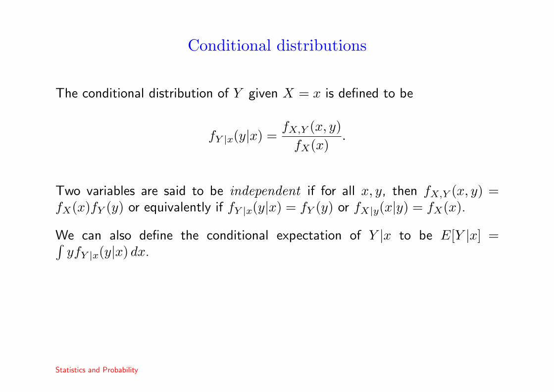
Conditional distributions

The conditional distribution of Y given X = x is defined to be

fY |x(y|x) =fX,Y (x, y)

fX(x).

Two variables are said to be independent if for all x, y, then fX,Y (x, y) =fX(x)fY (y) or equivalently if fY |x(y|x) = fY (y) or fX|y(x|y) = fX(x).

We can also define the conditional expectation of Y |x to be E[Y |x] =∫yfY |x(y|x) dx.


Covariance and correlation

It is useful to obtain a measure of the degree of relation between the twovariables. Such a measure is the correlation.

We can define the expectation of any function, g(X, Y ), in a similar way tothe univariate case,

E[g(X, Y )] =∫ ∫

g(x, y)fX,Y (x, y) dx dy.

In particular, the covariance is defined as

σX,Y = Cov[X, Y ] = E[XY ]− E[X]E[Y ].

Obviously, the units of the covariance are the product of the units of X andY . A scale free measure is the correlation,

ρX,Y = Corr[X, Y ] =σX,Y

σXσY


Properties of the correlation are as follows:

• −1 ≤ ρX,Y ≤ 1

• ρX,Y = 0 if X and Y are independent. (This is not necessarily true inreverse!)

• ρXY= 1 if there is an exact, positive relation between X and Y so that

Y = a + bX where b > 0.

• ρXY= −1 if there is an exact, negative relation between X and Y so that

Y = a + bX where b < 0.


The Cauchy Schwarz inequality

Theorem 11For two variables, X and Y , then

E[XY ]2 ≤ E[X2]E[Y 2].

Proof Let Z = aX − bY for real numbers a, b. Then

0 ≤ E[Z2] = a2E[X2]− 2abE[XY ] + b2E[Y 2]

and the right hand side is a quadratic in a with at most one real root. Thus,its discriminant must be non-positive so that if b 6= 0,

E[XY ]2 − E[X2]E[Y 2] ≤ 0.

The discriminant is zero iff the quadratic has a real root which occurs iffE[(aX − bY )2] = 0 for some a and b.


Example 21A random variable X has a beta distribution, X ∼ B(α, β), if

fX(x) =Γ(α + β)Γ(α)Γ(β)

xα−1(1− x)β−1 for 0 < x < 1.

The mean of X is E[X] = αα+β .

Suppose now that we toss a coin with probability P (heads) = X a total of ntimes and that we require the distribution of the number of heads, Y .

This is the beta-binomial distribution which is quite complicated:


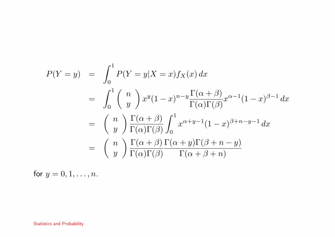
P (Y = y) =∫ 1

0

P (Y = y|X = x)fX(x) dx

=∫ 1

0

(ny

)xy(1− x)n−y Γ(α + β)

Γ(α)Γ(β)xα−1(1− x)β−1 dx

=(

ny

)Γ(α + β)Γ(α)Γ(β)

∫ 1

0

xα+y−1(1− x)β+n−y−1 dx

=(

ny

)Γ(α + β)Γ(α)Γ(β)

Γ(α + y)Γ(β + n− y)Γ(α + β + n)

for y = 0, 1, . . . , n.


We could try to calculate the mean of Y directly using the above probabilityfunction. However, this would be very complicated. There is a much easierway.

We could try to calculate the mean of Y directly using the above probabilityfunction. However, this would be very complicated. There is a much easierway.

E[Y ] = E[E[Y |X]]

= E[nX] because Y |X ∼ BI(n, X)

= nα

α + β.


The probability generating function for a sum of independent variables

Suppose that X1, . . . , Xn are independent with generating functions Gi(s) fors = 1, . . . , n. Let Y =

∑ni=1 Xi. Then

GY (s) = E[sY]

= E[s∑n

i=1 Xi

]=

n∏i=1

E[sXi]

by independence

=n∏

i=1

Gi(s)

Furthermore, if X1, . . . , Xn are identically distributed, with common generatingfunction GX(s), then

GY (s) = GX(s)n.


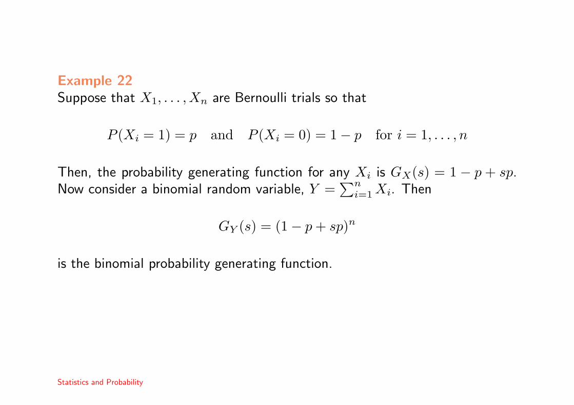
Example 22Suppose that X1, . . . , Xn are Bernoulli trials so that

P (Xi = 1) = p and P (Xi = 0) = 1− p for i = 1, . . . , n

Then, the probability generating function for any Xi is GX(s) = 1 − p + sp.Now consider a binomial random variable, Y =

∑ni=1 Xi. Then

GY (s) = (1− p + sp)n

is the binomial probability generating function.


Another useful property of pgfs

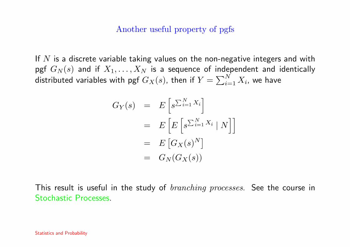
If N is a discrete variable taking values on the non-negative integers and withpgf GN(s) and if X1, . . . , XN is a sequence of independent and identically

distributed variables with pgf GX(s), then if Y =∑N

i=1 Xi, we have

GY (s) = E[s∑N

i=1 Xi

]= E

[E[s∑N

i=1 Xi | N]]

= E[GX(s)N

]= GN(GX(s))

This result is useful in the study of branching processes. See the course inStochastic Processes.


The moment generating function of a sum of independent variables

Suppose we have a sequence of independent variables, X1, X2, . . . , Xn withmgfs M1(s), . . . ,Mn(s). Then, if Y =

∑ni=1 Xi, it is easy to see that

MY (s) =n∏

i=1

Mi(s)

and if the variables are identically distributed with common mgf MX(s), then

MY (s) = MX(s)n.


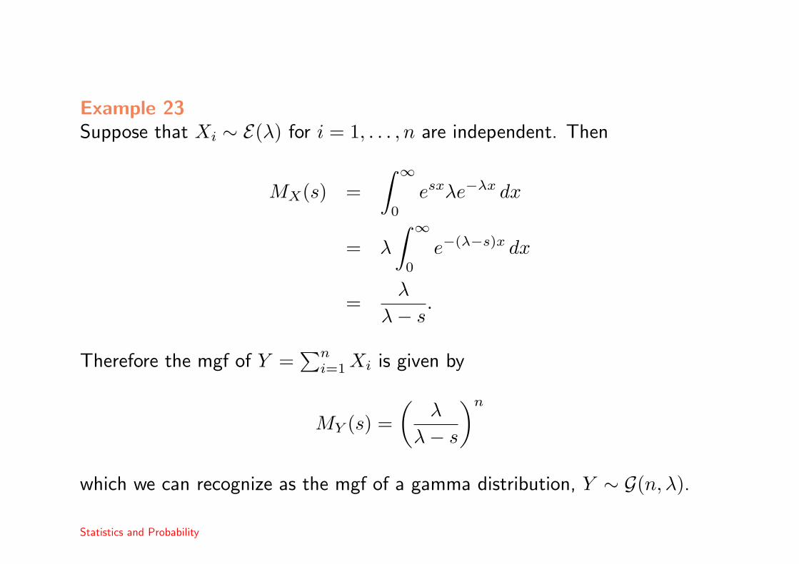
Example 23Suppose that Xi ∼ E(λ) for i = 1, . . . , n are independent. Then

MX(s) =∫ ∞

0

esxλe−λx dx

= λ

∫ ∞

0

e−(λ−s)x dx

=λ

λ− s.

Therefore the mgf of Y =∑n

i=1 Xi is given by

MY (s) =(

λ

λ− s

)n

which we can recognize as the mgf of a gamma distribution, Y ∼ G(n, λ).


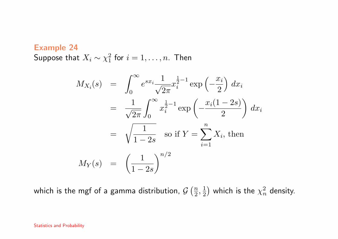
Example 24Suppose that Xi ∼ χ2

1 for i = 1, . . . , n. Then

MXi(s) =

∫ ∞

0

esxi1√2π

x12−1

i exp(−xi

2

)dxi

=1√2π

∫ ∞

0

x12−1

i exp(−xi(1− 2s)

2

)dxi

=

√1

1− 2sso if Y =

n∑i=1

Xi, then

MY (s) =(

11− 2s

)n/2

which is the mgf of a gamma distribution, G(

n2 , 1

2

)which is the χ2

n density.


Proof of the central limit theorem

For any variable, Y , with zero mean and unit variance and such that allmoments exist, then the moment generating function is

MY (s) = E[esY ] = 1 +s2

2+ o(s2).

Now assume that X1, . . . , Xn are a random sample from a distribution withmean µ and variance σ2. Then, we can define the standardized variables,Yi = Xi−µ

σ , which have mean 0 and variance 1 for i = 1, . . . , n and then

Zn =X − µ

σ/√

n=∑n

i=1 Yi√n

Now, suppose that MY (s) is the mgf of Yi, for i = 1, . . . , n. Then

MZn(s) = MY

(s/√

n)n


and therefore,

MZn(s) =(

1 +s2

2n+ o(s2/n)

)n

→ es2

2

which is the mgf of a normally distributed random variable.

and therefore,

MZn(s) =(

1 +s2

2n+ o(s2/n)

)n

→ es2

2

which is the mgf of a normally distributed random variable.

To make this result valid for variables that do not necessarily possessall their moments, then we can use essentially the same arguments butdefining the characteristic function CX(s) = E[eisX] instead of the momentgenerating function.


Sampling distributions

Often, in order to undertake inference, we wish to find the distribution of thesample mean, X or the sample variance, S2.

Theorem 13Suppose that we take a sample of size n from a population with mean µ andvariance σ2. Then

E[X] = µ

V [X] =σ2

n

E[S2] = σ2


Proof

E[X] =1nE

[n∑

i=1

Xi

]

=1n

∫. . .

∫ n∑i=1

xifX1,...,Xn(x1, . . . , xn) dx1, . . . , dxn

=1n

∫. . .

∫ n∑i=1

xifX1(x1) · · · fXn(xn) dx1, . . . , dxn by independence

=1n

n∑i=1

∫xifXi

(xi) dxi =1n

n∑i=1

µ = µ


V [X] =1

nV [

n∑i=1

Xi]

=1

n

n∑i=1

V [Xi] by independence

=nσ2

n= σ

2

E[S2] =

1

n− 1E

[n∑

i=1

(Xi − X)2

]

=1

n− 1E

[n∑

i=1

(Xi − µ + µ− X)2

]

=1

n− 1

n∑i=1

E[(Xi − µ)

2+ 2(Xi − µ)(µ− X) + (µ− X)

2]

=1

n− 1

(nσ

2 − 2nE[(X − µ)

2]

+ nσ2

n

)

=1

n− 1

(nσ

2 − σ2)

= σ2


The previous result shows that X and S2 are unbiased estimators of thepopulation mean and variance respectively.

A further important extension can be made if we assume that the data arenormally distributed.

Theorem 14If X1, . . . , Xn ∼ N (µ, σ2) then we have that X ∼ N (µ, σ2

n ).

Proof We can prove this using moment generating functions. First recall thatif Z ∼ N (0, 1), then X = µ + σZ ∼ N (µ, σ2) so that

MX(s) = E[esX] = E[esµ+sσZ] = esµE[esσZ] = esµMZ(σs).


Therefore, we have MX(s) = esµe(sσ)2

2 = esµ+s2σ2

2 .

Now, suppose that X1, . . . , Xn ∼ N (µ, σ2). Then

MX(s) = E[esX]

= E[e

sn

∑ni=1 Xi

]= MX

(s

n

)n

=(

esnµ+s2σ2

2n2

)n

= esµ+s2σ2/n

2

which is the mgf of a normal distribution, N (µ, σ2/n).


Probability - UC3Mhalweb.uc3m.es/esp/Personal/personas/mwiper/docencia/English/PhD... ·...

Documents

Transcript of Probability - UC3Mhalweb.uc3m.es/esp/Personal/personas/mwiper/docencia/English/PhD... ·...