
Basic notions of probability theory: continuous probability distributions · Basic notions of...
58
Piero Baraldi Basic notions of probability theory: • continuous probability distributions
Transcript of Basic notions of probability theory: continuous probability distributions · Basic notions of...

Piero Baraldi
Basic notions of probability theory:
• continuous probability distributions
• discrete probability distributions
Probability distributions for reliability, safety and risk analysis:
• continuous probability distributions
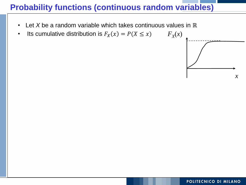
• Let X be a random variable which takes continuous values in ℝ
• Its cumulative distribution is 𝐹𝑋 𝑥 = 𝑃(𝑋 ≤ 𝑥)
Probability functions (continuous random variables)
FX(x)
x
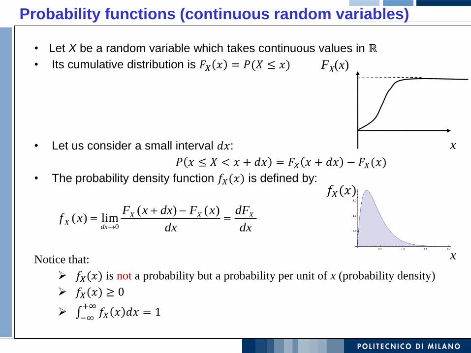
• Let X be a random variable which takes continuous values in ℝ
• Its cumulative distribution is 𝐹𝑋 𝑥 = 𝑃(𝑋 ≤ 𝑥)
• Let us consider a small interval 𝑑𝑥:
𝑃 𝑥 ≤ 𝑋 < 𝑥 + 𝑑𝑥 = 𝐹𝑋 𝑥 + 𝑑𝑥 − 𝐹𝑋(𝑥)
• The probability density function 𝑓𝑋(𝑥) is defined by:
Notice that:
➢ 𝑓𝑋(𝑥) is not a probability but a probability per unit of x (probability density)
➢ 𝑓𝑋(𝑥) ≥ 0
➢ ∞−+∞
𝑓𝑋 𝑥 𝑑𝑥 = 1
dx
dF
dx
xFdxxFxf XXX
dxX
)()(lim)(
0
Probability functions (continuous random variables)
FX(x)
x
x
𝑓𝑋(𝑥)
Summary measures:percentiles, median, mean, variance
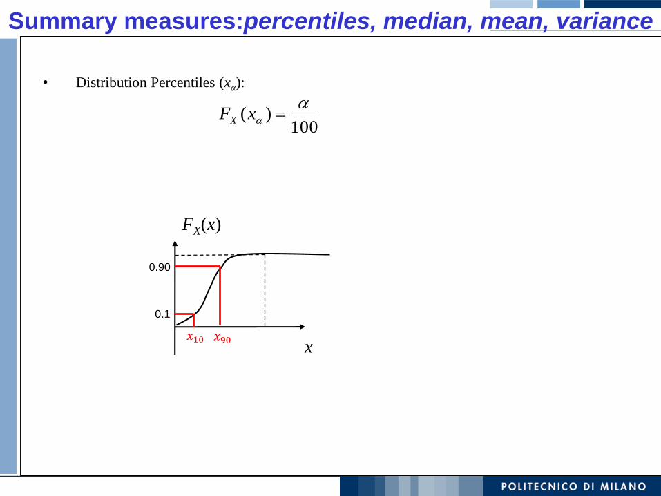
• Distribution Percentiles (xα):
100)(
xFX
FX(x)
x𝑥10 𝑥90
0.1
0.90
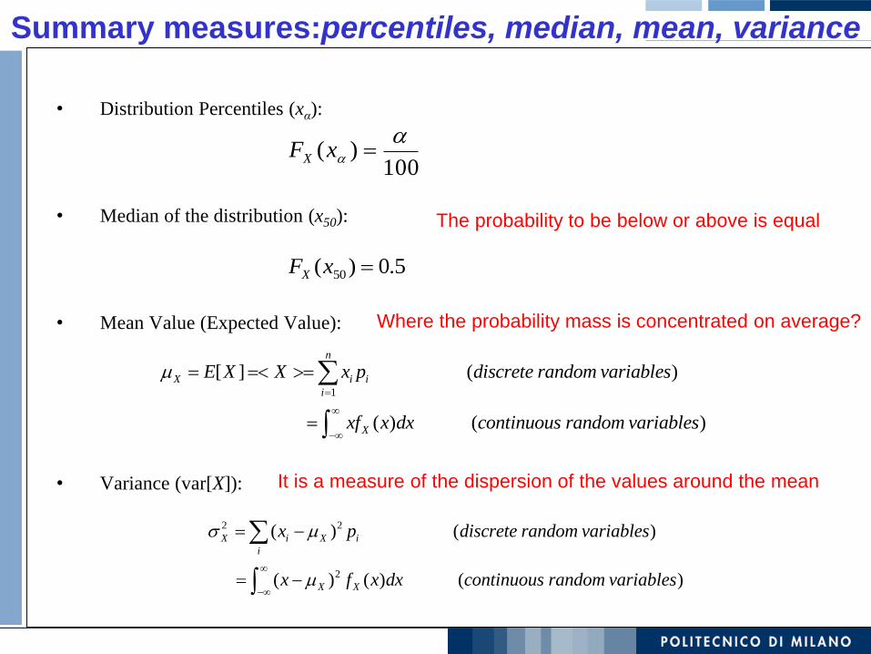
Summary measures:percentiles, median, mean, variance
• Distribution Percentiles (xα):
• Median of the distribution (x50):
• Mean Value (Expected Value):
• Variance (var[X]):
100)(
xFX
5.0)( 50 xFX
1
[ ] ( )
( ) ( )
n
X i i
i
X
E X X x p discrete random variables
xf x dx continuous random variables
2 2
2
( ) ( )
( ) ( ) ( )
X i X i
i
X X
x p discrete random variables
x f x dx continuous random variables
It is a measure of the dispersion of the values around the mean
The probability to be below or above is equal
Where the probability mass is concentrated on average?
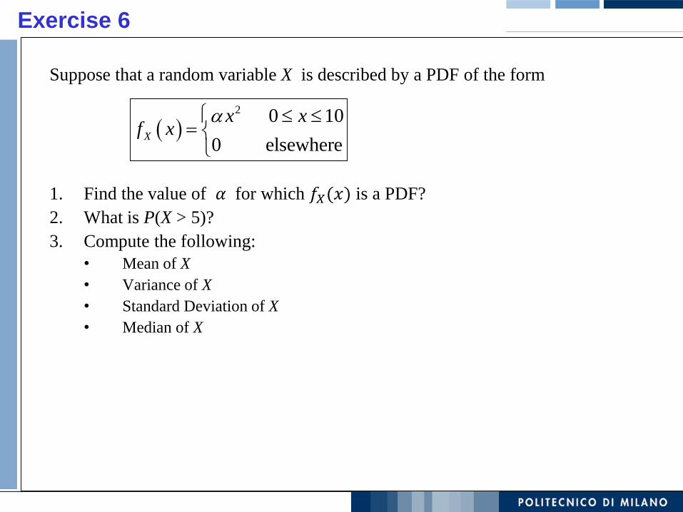
Exercise 6
Suppose that a random variable X is described by a PDF of the form
1. Find the value of 𝛼 for which 𝑓𝑋(𝑥) is a PDF?
2. What is P(X > 5)?
3. Compute the following:
• Mean of X
• Variance of X
• Standard Deviation of X
• Median of X
2 0 10
0 elsewhereX
x xf x
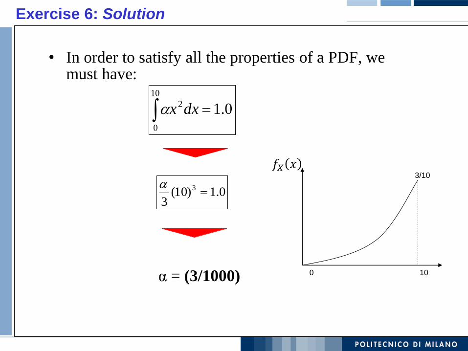
Exercise 6: Solution
• In order to satisfy all the properties of a PDF, we must have:
α = (3/1000)
10
0
2 0.1dxx
0.1)10(3
3
3/10
100
𝑓𝑋 𝑥
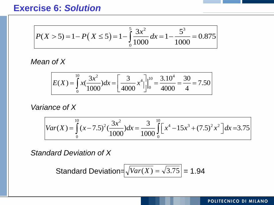
Exercise 6: Solution
5 2 3
0
3 5( 5) 1 5 1 1 0.875
1000 1000
xP X P X dx
Mean of X
Variance of X
Standard Deviation of X
Standard Deviation= = 1.94
10 2 410
4
00
3 3 3.10 30( ) ( ) 7.50
1000 4000 4000 4|
xE X x dx x
10 1022 4 3 2 2
0 0
3 3( ) ( 7.5) ( ) 15 (7.5) 3.75
1000 1000
xVar X x dx x x x dx
75.3)( XVar
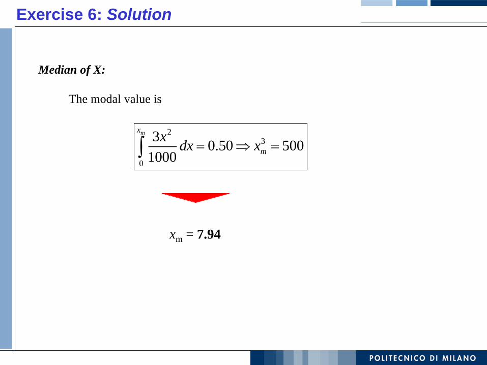
Exercise 6: Solution
Median of X:
The modal value is
23
0
30.50 500
1000
mx
m
xdx x
xm = 7.94
Reliability
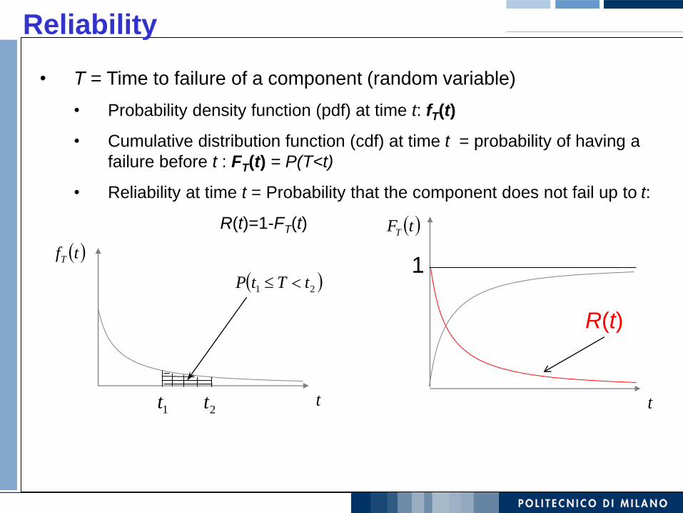
• T = Time to failure of a component (random variable)
• Probability density function (pdf) at time t: fT(t)
• Cumulative distribution function (cdf) at time t = probability of having a
failure before t : FT(t) = P(T<t)
• Reliability at time t = Probability that the component does not fail up to t:
R(t)=1-FT(t)
tfT
t1t 2t
21 tTtP
tFT
t
1
R(t)
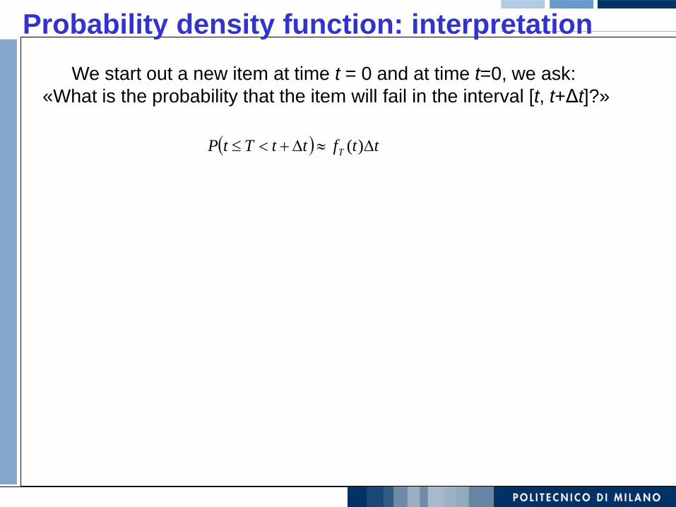
Probability density function: interpretation
ttfttTtP T )(
We start out a new item at time t = 0 and at time t=0, we ask:
«What is the probability that the item will fail in the interval [t, t+Δt]?»
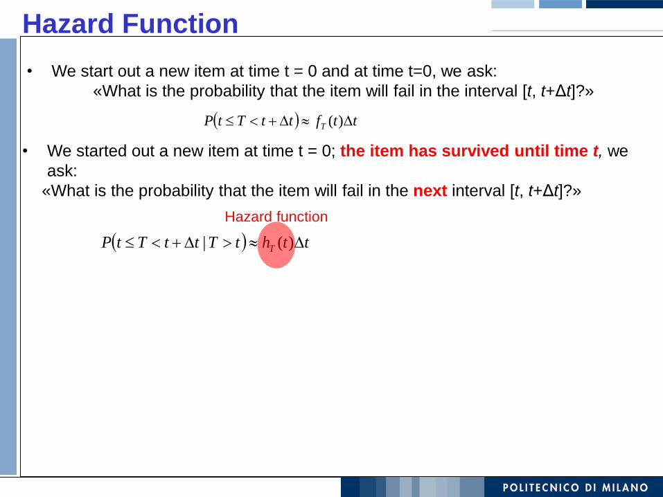
Hazard Function
ttfttTtP T )(
• We start out a new item at time t = 0 and at time t=0, we ask:
«What is the probability that the item will fail in the interval [t, t+Δt]?»
tthtTttTtP T )(|
• We started out a new item at time t = 0; the item has survived until time t, we
ask:
«What is the probability that the item will fail in the next interval [t, t+Δt]?»
Hazard function
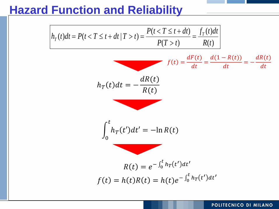
Hazard Function and Reliability
)(
)(
)(
)()|()(
tR
dttf
tTP
dttTtPtTdttTtPdtth T
T
ℎ𝑇 𝑡 𝑑𝑡 = −𝑑𝑅(𝑡)
𝑅(𝑡)
න0
𝑡
ℎ𝑇 𝑡′ 𝑑𝑡′ = −ln𝑅(𝑡)
𝑅 𝑡 = 𝑒− 0𝑡ℎ𝑇 𝑡′ 𝑑𝑡′
𝑓 𝑡 = ℎ 𝑡 𝑅 𝑡 = ℎ(𝑡)𝑒− 0𝑡ℎ𝑇 𝑡′ 𝑑𝑡′
𝑓 𝑡 =𝑑𝐹(𝑡)
𝑑𝑡=𝑑(1 − 𝑅(𝑡))
𝑑𝑡= −
𝑑𝑅(𝑡)
𝑑𝑡
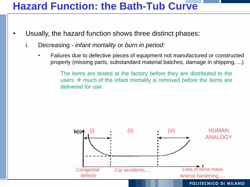
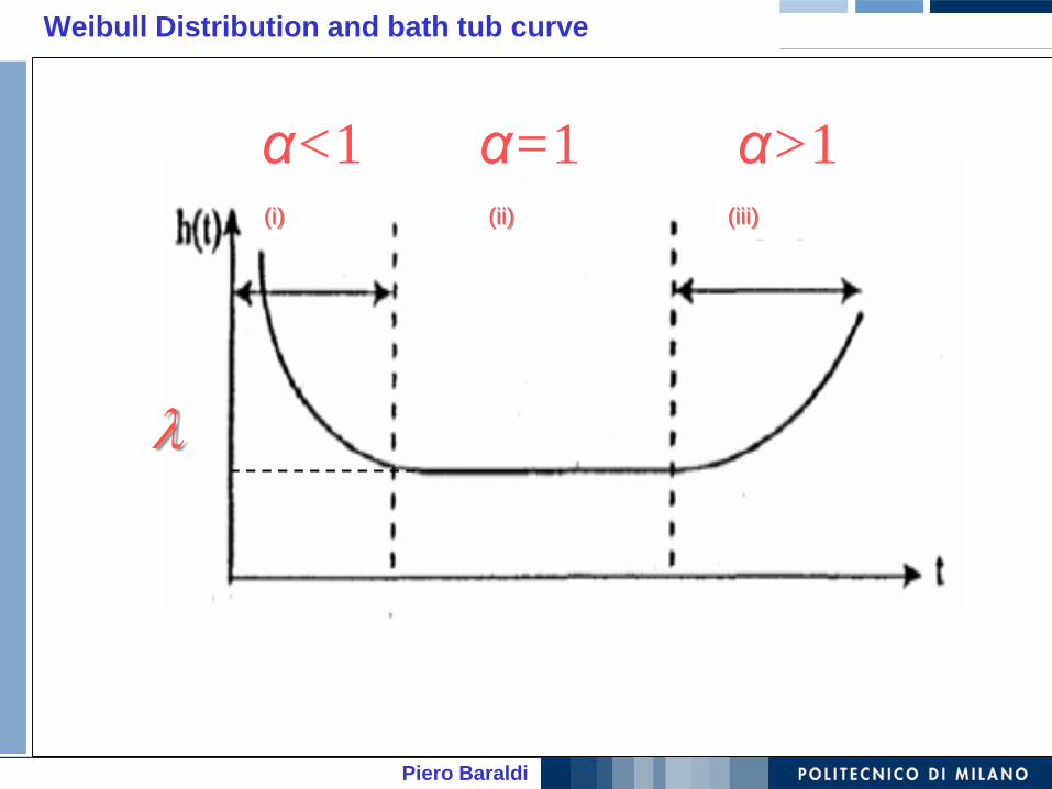
Hazard Function: the Bath-Tub Curve
• Usually, the hazard function shows three distinct phases:
i. Decreasing - infant mortality or burn in period:
• Failures due to defective pieces of equipment not manufactured or constructed
properly (missing parts, substandard material batches, damage in shipping, ...)
(i) (iii)(ii) HUMAN
ANALOGY
Congenital
defectsCar accidents,… Loss of bone mass
Arterial hardening,…
The items are tested at the factory before they are distributed to the
users much of the infant mortality is removed before the items are
delivered for use.
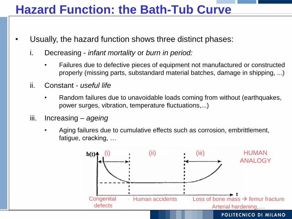
Hazard Function: the Bath-Tub Curve
• Usually, the hazard function shows three distinct phases:
i. Decreasing - infant mortality or burn in period:
• Failures due to defective pieces of equipment not manufactured or constructed
properly (missing parts, substandard material batches, damage in shipping, ...)
ii. Constant - useful life
• Random failures due to unavoidable loads coming from without (earthquakes,
power surges, vibration, temperature fluctuations,...)
iii. Increasing – ageing
• Aging failures due to cumulative effects such as corrosion, embrittlement,
fatigue, cracking, …
(i) (iii)(ii) HUMAN
ANALOGY
Congenital
defectsHuman accidents Loss of bone mass femur fracture
Arterial hardening,…
Univariate continuous probability distributions:
1) exponential distribution
2) Weibull distribution
3) Normal distribution
Piero Baraldi
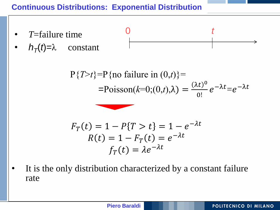
Continuous Distributions: Exponential Distribution
• T=failure time
• hT(t)=λ constant
0 t
P{T>t}=P{no failure in (0,t)}=
=Poisson(k=0;(0,t),λ) =λ𝑡 0
0!𝑒−λ𝑡=𝑒−λ𝑡
𝐹𝑇 𝑡 = 1 − 𝑃 𝑇 > 𝑡 = 1 − 𝑒−𝜆𝑡
𝑅 𝑡 = 1 − 𝐹𝑇 𝑡 = 𝑒−𝜆𝑡
𝑓𝑇(𝑡) = 𝜆𝑒−𝜆𝑡
• It is the only distribution characterized by a constant failurerate

Piero Baraldi
Exponential Distribution and bath tub curve
(i) (iii)(ii)
Piero Baraldi
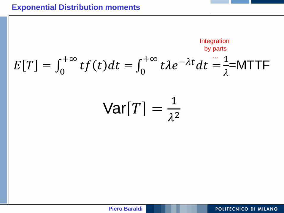
Exponential Distribution moments
𝐸 𝑇 = 0+∞
𝑡𝑓 𝑡 𝑑𝑡 0=+∞
𝑡𝜆𝑒−𝜆𝑡𝑑𝑡 =1
𝜆=MTTF
Var 𝑇 =1
𝜆2
Integration
by parts
…
Piero Baraldi
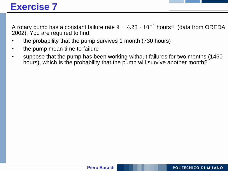
Exercise 7
A rotary pump has a constant failure rate 𝜆 = 4.28 ∙ 10−4 hours-1 (data from OREDA 2002). You are required to find:
• the probability that the pump survives 1 month (730 hours)
• the pump mean time to failure
• suppose that the pump has been working without failures for two months (1460 hours), which is the probability that the pump will survive another month?
Piero Baraldi
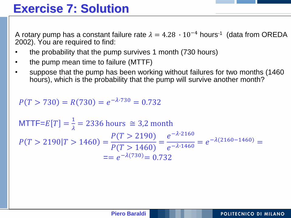
Exercise 7: Solution
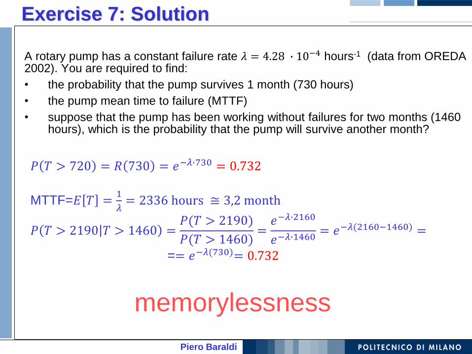
A rotary pump has a constant failure rate 𝜆 = 4.28 ∙ 10−4 hours-1 (data from OREDA 2002). You are required to find:
• the probability that the pump survives 1 month (730 hours)
• the pump mean time to failure (MTTF)
• suppose that the pump has been working without failures for two months (1460 hours), which is the probability that the pump will survive another month?
𝑃 𝑇 > 730 = 𝑅 730 = 𝑒−𝜆∙730 = 0.732
MTTF=𝐸 𝑇 =1
𝜆= 2336 hours ≅ 3,2 month
𝑃 𝑇 > 2190 𝑇 > 1460 =𝑃(𝑇 > 2190)
𝑃(𝑇 > 1460)=𝑒−𝜆∙2160
𝑒−𝜆∙1460= 𝑒−𝜆(2160−1460) =
== 𝑒−𝜆(730)= 0.732
Piero Baraldi
Exercise 7: Solution
A rotary pump has a constant failure rate 𝜆 = 4.28 ∙ 10−4 hours-1 (data from OREDA 2002). You are required to find:
• the probability that the pump survives 1 month (730 hours)
• the pump mean time to failure (MTTF)
• suppose that the pump has been working without failures for two months (1460 hours), which is the probability that the pump will survive another month?
𝑃 𝑇 > 720 = 𝑅 730 = 𝑒−𝜆∙730 = 0.732
MTTF=𝐸 𝑇 =1
𝜆= 2336 hours ≅ 3,2 month
𝑃 𝑇 > 2190 𝑇 > 1460 =𝑃(𝑇 > 2190)
𝑃(𝑇 > 1460)=𝑒−𝜆∙2160
𝑒−𝜆∙1460= 𝑒−𝜆(2160−1460) =
== 𝑒−𝜆(730)= 0.732
memorylessness
Piero Baraldi
Exponential distribution: memorylessness
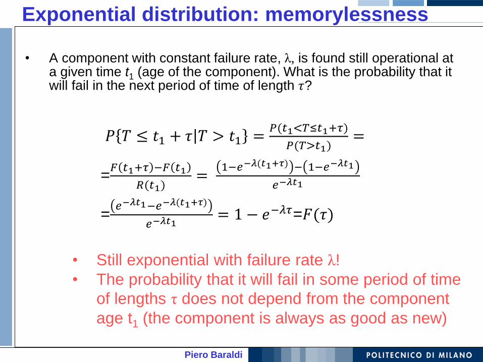
• A component with constant failure rate, λ, is found still operational ata given time t1 (age of the component). What is the probability that itwill fail in the next period of time of length 𝜏?
𝑃 𝑇 ≤ 𝑡1 + 𝜏 𝑇 > 𝑡1 =𝑃(𝑡1<𝑇≤𝑡1+𝜏)
𝑃(𝑇>𝑡1)=
=𝐹 𝑡1+𝜏 −𝐹 𝑡1
𝑅(𝑡1)=
1−𝑒−𝜆(𝑡1+𝜏) − 1−𝑒−𝜆𝑡1
𝑒−𝜆𝑡1
=𝑒−𝜆𝑡1−𝑒−𝜆(𝑡1+𝜏)
𝑒−𝜆𝑡1= 1 − 𝑒−𝜆𝜏=𝐹(𝜏)
• Still exponential with failure rate λ!
• The probability that it will fail in some period of time
of lengths τ does not depend from the component
age t1 (the component is always as good as new)
Piero Baraldi
Statistical distribution of the failure times of N components with constant failure rate
0 25 50 75 1001251501752002252502753003253503754004254504755005255505756006256506757000
0.05
0.1
0.15
0.2
0.25
t
50
100
150
200MTTF=100
0 25 50 75
𝐸[𝐹]
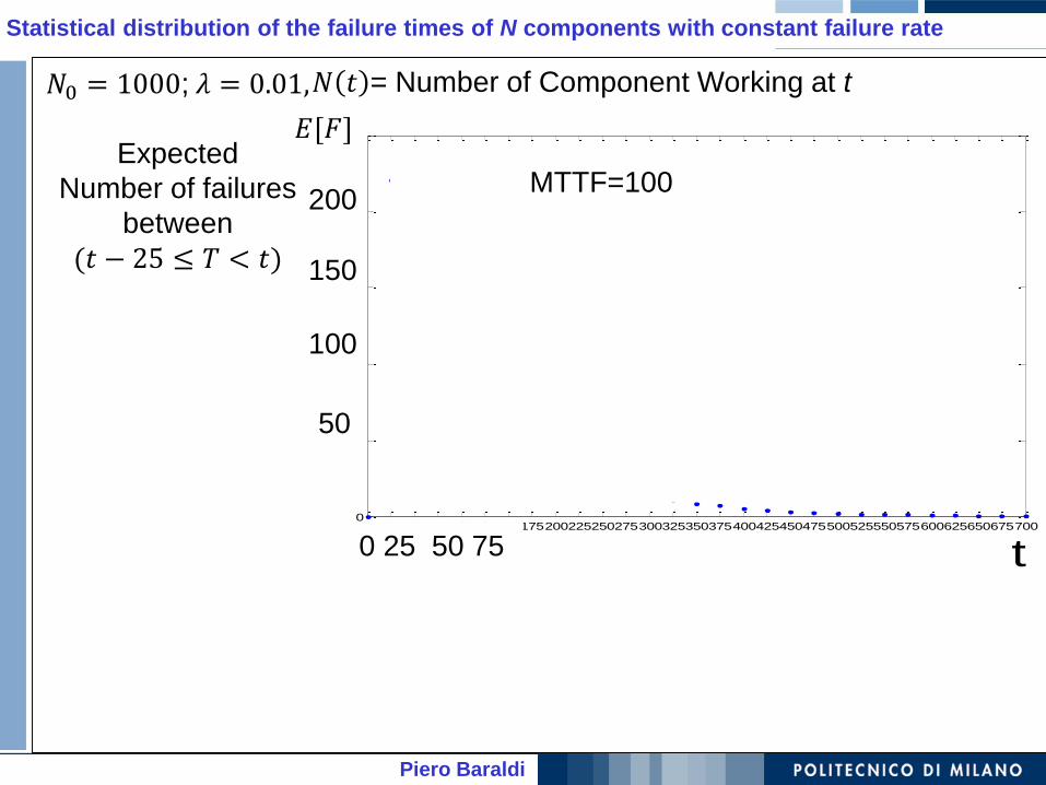
𝑁0 = 1000; 𝜆 = 0.01,
Expected
Number of failures
between
(𝑡 − 25 ≤ 𝑇 < 𝑡)
𝑁 𝑡 = Number of Component Working at t
Piero Baraldi
Statistical distribution of the failure times of N components with constant failure rate
0 25 50 75 1001251501752002252502753003253503754004254504755005255505756006256506757000
0.05
0.1
0.15
0.2
0.25
t
50
100
150
200MTTF=100
0 25 50 75
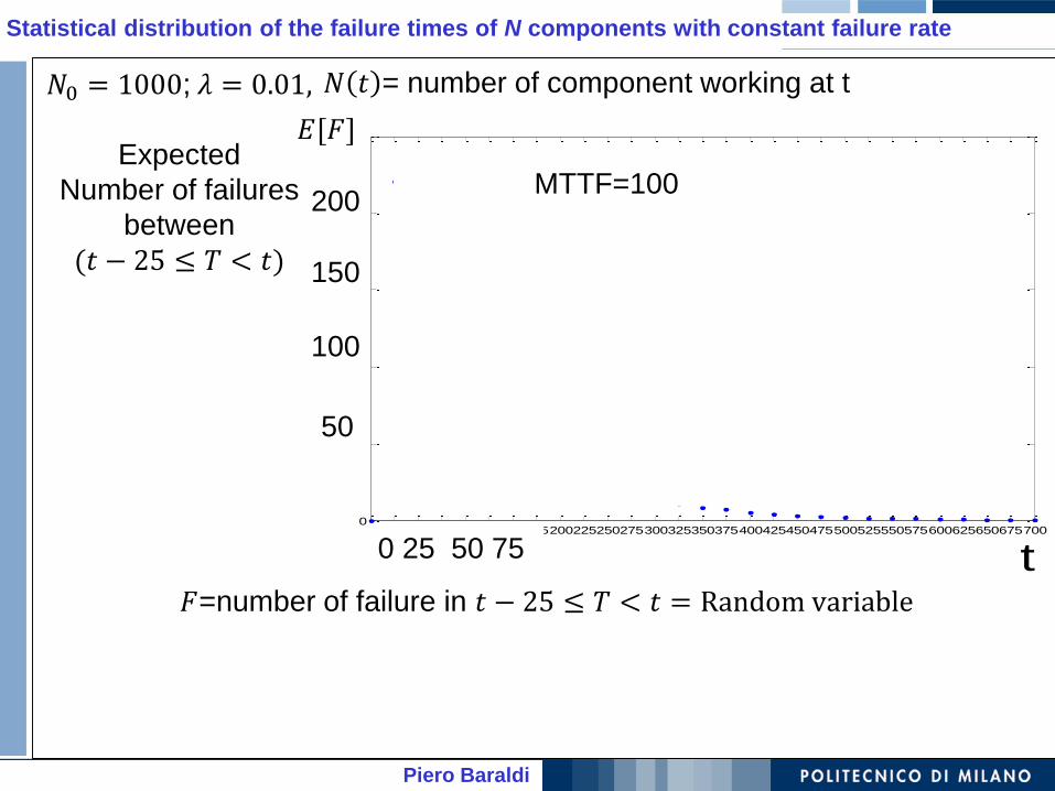
𝐹=number of failure in 𝑡 − 25 ≤ 𝑇 < 𝑡 = Random variable
𝐸[𝐹]
𝑁0 = 1000; 𝜆 = 0.01,
Expected
Number of failures
between
(𝑡 − 25 ≤ 𝑇 < 𝑡)
𝑁 𝑡 = number of component working at t
Piero Baraldi
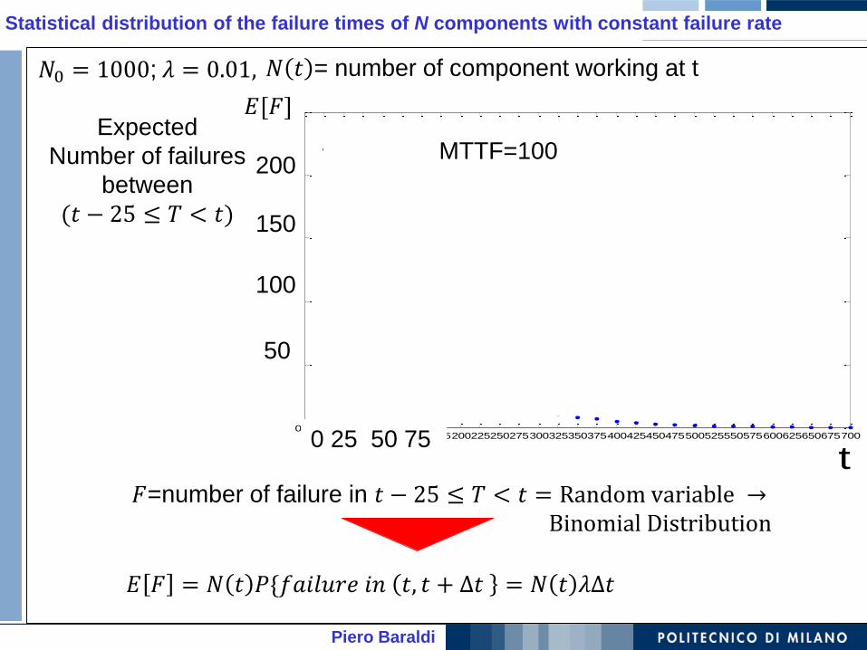
Statistical distribution of the failure times of N components with constant failure rate
0 25 50 75 1001251501752002252502753003253503754004254504755005255505756006256506757000
0.05
0.1
0.15
0.2
0.25
t
50
100
150
200MTTF=100
0 25 50 75
𝐹=number of failure in 𝑡 − 25 ≤ 𝑇 < 𝑡 = Random variable →Binomial Distribution
𝐸[𝐹]
𝐸 𝐹 = 𝑁 𝑡 𝑃{𝑓𝑎𝑖𝑙𝑢𝑟𝑒 𝑖𝑛 𝑡, 𝑡 + Δ𝑡 = 𝑁 𝑡 𝜆Δ𝑡
𝑁0 = 1000; 𝜆 = 0.01,
Expected
Number of failures
between
(𝑡 − 25 ≤ 𝑇 < 𝑡)
𝑁 𝑡 = number of component working at t
Piero Baraldi
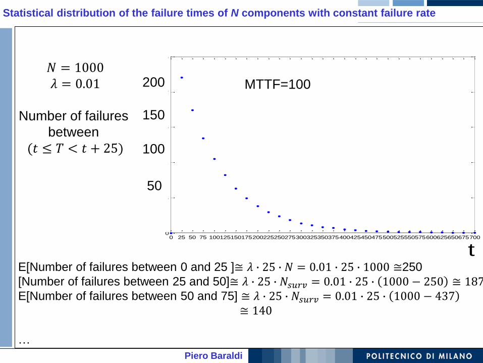
Statistical distribution of the failure times of N components with constant failure rate
0 25 50 75 1001251501752002252502753003253503754004254504755005255505756006256506757000
0.05
0.1
0.15
0.2
0.25
t
50
100
150
200
E[Number of failures between 0 and 25 ]≅ 𝜆 ∙ 25 ∙ 𝑁 = 0.01 ∙ 25 ∙ 1000 ≅250
[Number of failures between 25 and 50]≅ 𝜆 ∙ 25 ∙ 𝑁𝑠𝑢𝑟𝑣 = 0.01 ∙ 25 ∙ 1000 − 250 ≅ 187E[Number of failures between 50 and 75] ≅ 𝜆 ∙ 25 ∙ 𝑁𝑠𝑢𝑟𝑣 = 0.01 ∙ 25 ∙ 1000 − 437
≅ 140
…
MTTF=100
𝑁 = 1000𝜆 = 0.01
Number of failures
between
(𝑡 ≤ 𝑇 < 𝑡 + 25)
Univariate continuous probability distributions:
1) exponential distribution
2) Weibull distribution
3) Normal distribution
3030Piero Baraldi
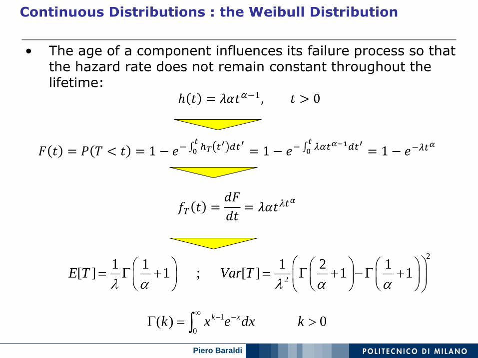
𝐹 𝑡 = 𝑃 𝑇 < 𝑡 = 1 − 𝑒− 0𝑡ℎ𝑇 𝑡′ 𝑑𝑡′ = 1 − 𝑒− 0
𝑡𝜆𝛼𝑡𝛼−1𝑑𝑡′ = 1 − 𝑒−𝜆𝑡
𝛼
𝑓𝑇 𝑡 =𝑑𝐹
𝑑𝑡= 𝜆𝛼𝑡𝜆𝑡
𝛼
• The age of a component influences its failure process so that the hazard rate does not remain constant throughout the lifetime:
ℎ 𝑡 = 𝜆𝛼𝑡𝛼−1, 𝑡 > 0
2
2
1 1 1 2 1[ ] 1 ; [ ] 1 1E T Var T
0
1 0)( kdxexk xk
Continuous Distributions : the Weibull Distribution
Piero Baraldi
Weibull Distribution and bath tub curve
(i) (iii)(ii)
α<1 α>1α=1
Univariate continuous probability distributions:
1) exponential distribution
2) Weibull distribution
3) Normal distribution
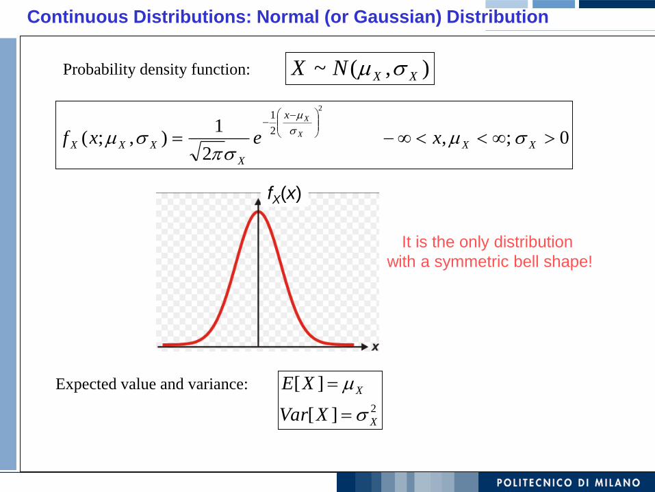
Continuous Distributions: Normal (or Gaussian) Distribution
Probability density function:
Expected value and variance:
2][
][
X
X
XVar
XE
0;,2
1),;(
2
2
1
XX
x
X
XXX xexf X
X
),(~ XXNX
It is the only distribution
with a symmetric bell shape!
fX(x)
Piero Baraldi
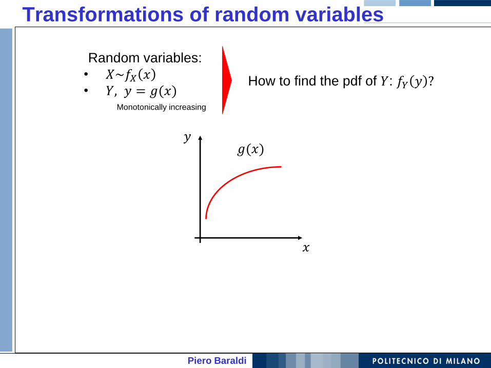
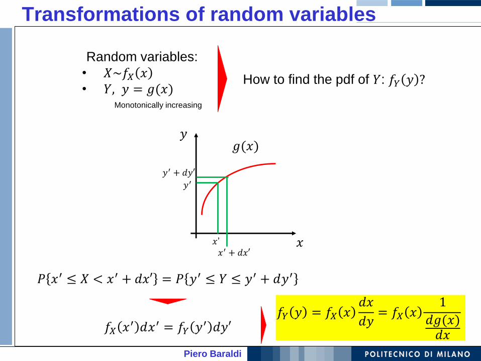
Transformations of random variables
Random variables:
• 𝑋~𝑓𝑋 𝑥• 𝑌, 𝑦 = 𝑔(𝑥)
How to find the pdf of 𝑌: 𝑓𝑌 𝑦 ?
𝑥
𝑦𝑔(𝑥)
Monotonically increasing
Piero Baraldi
Transformations of random variables
Random variables:
• 𝑋~𝑓𝑋 𝑥• 𝑌, 𝑦 = 𝑔(𝑥)
How to find the pdf of 𝑌: 𝑓𝑌 𝑦 ?
𝑥
𝑦𝑔(𝑥)
Monotonically increasing
𝑥’
𝑥′ + 𝑑𝑥′
𝑦′ + 𝑑𝑦′
𝑦′
𝑃 𝑥′ ≤ 𝑋 < 𝑥′ + 𝑑𝑥′ = 𝑃 𝑦′ ≤ 𝑌 ≤ 𝑦′ + 𝑑𝑦′
𝑓𝑋 𝑥′ 𝑑𝑥′ = 𝑓𝑌 𝑦′ 𝑑𝑦′𝑓𝑌 𝑦 = 𝑓𝑋 𝑥
𝑑𝑥
𝑑𝑦= 𝑓𝑋 𝑥
1
𝑑𝑔(𝑥)𝑑𝑥
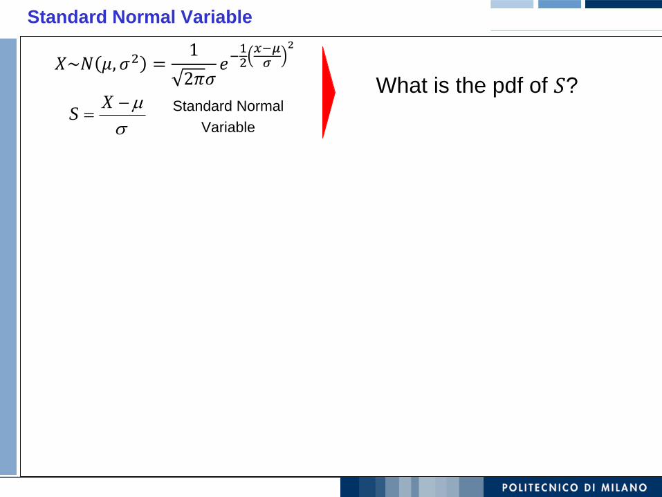
Standard Normal Variable
XS
What is the pdf of 𝑆?𝑋~𝑁 𝜇, 𝜎2 =
1
2𝜋𝜎𝑒−12𝑥−𝜇𝜎
2
Standard Normal
Variable
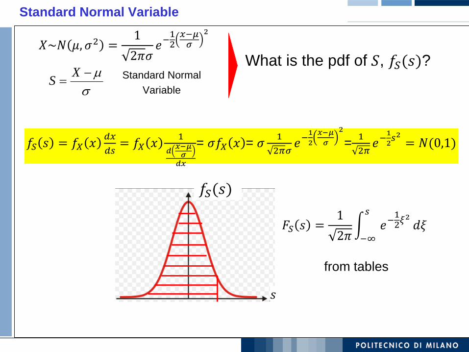
Standard Normal Variable
XS
What is the pdf of 𝑆, 𝑓𝑆(𝑠)?𝑋~𝑁 𝜇, 𝜎2 =
1
2𝜋𝜎𝑒−12𝑥−𝜇𝜎
2
Standard Normal
Variable
𝑓𝑆 𝑠 = 𝑓𝑋 𝑥𝑑𝑥
𝑑𝑠= 𝑓𝑋 𝑥
1
𝑑𝑥−𝜇𝜎
𝑑𝑥
= 𝜎𝑓𝑋 𝑥 = 𝜎1
2𝜋𝜎𝑒−1
2
𝑥−𝜇
𝜎
2
=1
2𝜋𝑒−
1
2𝑠2 = 𝑁(0,1)
𝑠
𝑓𝑆(𝑠)
𝐹𝑆 𝑠 =1
2𝜋න−∞
𝑠
𝑒−12𝜉
2𝑑𝜉
from tables
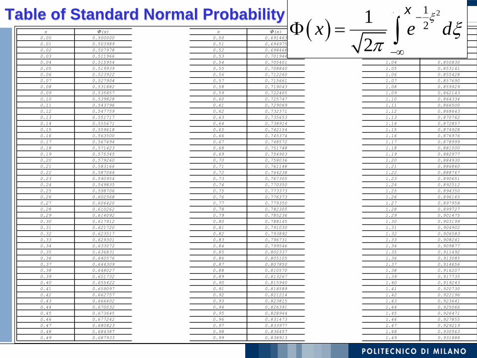
Table of Standard Normal Probabilityx (x) x (x) x (x)
0.00 0.500000 0.50 0.691463 1.00 0.841345
0.01 0.503989 0.51 0.694975 1.01 0.843752
0.02 0.507978 0.52 0.698468 1.02 0.846136
0.03 0.511966 0.53 0.701944 1.03 0.848495
0.04 0.515954 0.54 0.705401 1.04 0.850830
0.05 0.519939 0.55 0.708840 1.05 0.853141
0.06 0.523922 0.56 0.712260 1.06 0.855428
0.07 0.527904 0.57 0.715661 1.07 0.857690
0.08 0.531882 0.58 0.719043 1.08 0.859929
0.09 0.535857 0.59 0.722405 1.09 0.862143
0.10 0.539828 0.60 0.725747 1.10 0.864334
0.11 0.543796 0.61 0.729069 1.11 0.866500
0.12 0.547759 0.62 0.732371 1.12 0.868643
0.13 0.551717 0.63 0.735653 1.13 0.870762
0.14 0.555671 0.64 0.738914 1.14 0.872857
0.15 0.559618 0.65 0.742154 1.15 0.874928
0.16 0.563500 0.66 0.745374 1.16 0.876976
0.17 0.567494 0.67 0.748572 1.17 0.878999
0.18 0.571423 0.68 0.751748 1.18 0.881000
0.19 0.575345 0.69 0.754903 1.19 0.882977
0.20 0.579260 0.70 0.758036 1.20 0.884930
0.21 0.583166 0.71 0.761148 1.21 0.886860
0.22 0.587064 0.72 0.764238 1.22 0.888767
0.23 0.590954 0.73 0.767305 1.23 0.890651
0.24 0.549835 0.74 0.770350 1.24 0.892512
0.25 0.598706 0.75 0.773373 1.25 0.894350
0.26 0.602568 0.76 0.776373 1.26 0.896165
0.27 0.606420 0.77 0.779350 1.27 0.897958
0.28 0.610262 0.78 0.782305 1.28 0.899727
0.29 0.614092 0.79 0.785236 1.29 0.901475
0.30 0.617912 0.80 0.788145 1.30 0.903199
0.31 0.621720 0.81 0.791030 1.31 0.904902
0.32 0.623517 0.82 0.793892 1.32 0.906583
0.33 0.629301 0.83 0.796731 1.33 0.908241
0.34 0.633072 0.84 0.799546 1.34 0.909877
0.35 0.636831 0.85 0.802337 1.35 0.911492
0.36 0.640576 0.86 0.805105 1.36 0.913085
0.37 0.644309 0.87 0.807850 1.37 0.914656
0.38 0.648027 0.88 0.810570 1.38 0.916207
0.39 0.651732 0.89 0.813267 1.39 0.917735
0.40 0.655422 0.90 0.815940 1.40 0.919243
0.41 0.659097 0.91 0.818589 1.41 0.920730
0.42 0.662757 0.92 0.821214 1.42 0.922196
0.43 0.666402 0.93 0.823815 1.43 0.923641
0.44 0.670032 0.94 0.826391 1.44 0.925066
0.45 0.673645 0.95 0.828944 1.45 0.926471
0.46 0.677242 0.96 0.831473 1.46 0.927855
0.47 0.680823 0.97 0.833977 1.47 0.929219
0.48 0.684387 0.98 0.836457 1.48 0.930563
0.49 0.687933 0.99 0.838913 1.49 0.931888
21
21
2x e d
x
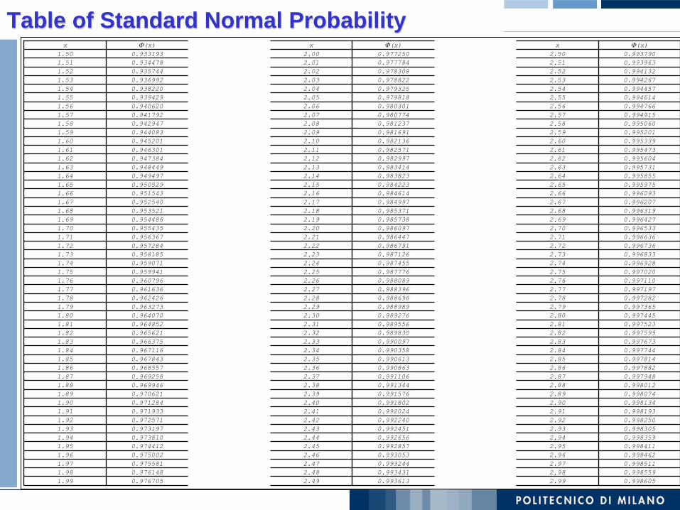
x (x) x (x) x (x)
1.50 0.933193 2.00 0.977250 2.50 0.993790
1.51 0.934478 2.01 0.977784 2.51 0.993963
1.52 0.935744 2.02 0.978308 2.52 0.994132
1.53 0.936992 2.03 0.978822 2.53 0.994267
1.54 0.938220 2.04 0.979325 2.54 0.994457
1.55 0.939429 2.05 0.979818 2.55 0.994614
1.56 0.940620 2.06 0.980301 2.56 0.994766
1.57 0.941792 2.07 0.980774 2.57 0.994915
1.58 0.942947 2.08 0.981237 2.58 0.995060
1.59 0.944083 2.09 0.981691 2.59 0.995201
1.60 0.945201 2.10 0.982136 2.60 0.995339
1.61 0.946301 2.11 0.982571 2.61 0.995473
1.62 0.947384 2.12 0.982997 2.62 0.995604
1.63 0.948449 2.13 0.983414 2.63 0.995731
1.64 0.949497 2.14 0.983823 2.64 0.995855
1.65 0.950529 2.15 0.984223 2.65 0.995975
1.66 0.951543 2.16 0.984614 2.66 0.996093
1.67 0.952540 2.17 0.984997 2.67 0.996207
1.68 0.953521 2.18 0.985371 2.68 0.996319
1.69 0.954486 2.19 0.985738 2.69 0.996427
1.70 0.955435 2.20 0.986097 2.70 0.996533
1.71 0.956367 2.21 0.986447 2.71 0.996636
1.72 0.957284 2.22 0.986791 2.72 0.996736
1.73 0.958185 2.23 0.987126 2.73 0.996833
1.74 0.959071 2.24 0.987455 2.74 0.996928
1.75 0.959941 2.25 0.987776 2.75 0.997020
1.76 0.960796 2.26 0.988089 2.76 0.997110
1.77 0.961636 2.27 0.988396 2.77 0.997197
1.78 0.962426 2.28 0.988696 2.78 0.997282
1.79 0.963273 2.29 0.988989 2.79 0.997365
1.80 0.964070 2.30 0.989276 2.80 0.997445
1.81 0.964852 2.31 0.989556 2.81 0.997523
1.82 0.965621 2.32 0.989830 2.82 0.997599
1.83 0.966375 2.33 0.990097 2.83 0.997673
1.84 0.967116 2.34 0.990358 2.84 0.997744
1.85 0.967843 2.35 0.990613 2.85 0.997814
1.86 0.968557 2.36 0.990863 2.86 0.997882
1.87 0.969258 2.37 0.991106 2.87 0.997948
1.88 0.969946 2.38 0.991344 2.88 0.998012
1.89 0.970621 2.39 0.991576 2.89 0.998074
1.90 0.971284 2.40 0.991802 2.90 0.998134
1.91 0.971933 2.41 0.992024 2.91 0.998193
1.92 0.972571 2.42 0.992240 2.92 0.998250
1.93 0.973197 2.43 0.992451 2.93 0.998305
1.94 0.973810 2.44 0.992656 2.94 0.998359
1.95 0.974412 2.45 0.992857 2.95 0.998411
1.96 0.975002 2.46 0.993053 2.96 0.998462
1.97 0.975581 2.47 0.993244 2.97 0.998511
1.98 0.976148 2.48 0.993431 2.98 0.998559
1.99 0.976705 2.49 0.993613 2.99 0.998605
Table of Standard Normal Probability
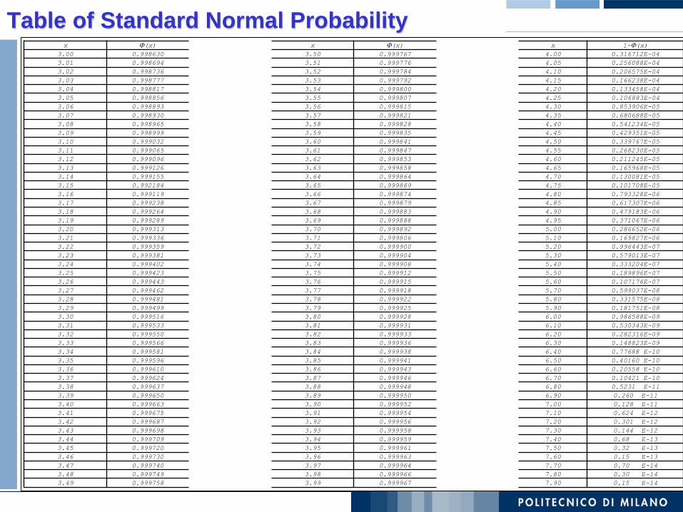
x (x) x (x) x 1-(x)
3.00 0.998630 3.50 0.999767 4.00 0.316712E-04
3.01 0.998694 3.51 0.999776 4.05 0.256088E-04
3.02 0.998736 3.52 0.999784 4.10 0.206575E-04
3.03 0.998777 3.53 0.999792 4.15 0.166238E-04
3.04 0.998817 3.54 0.999800 4.20 0.133458E-04
3.05 0.998856 3.55 0.999807 4.25 0.106883E-04
3.06 0.998893 3.56 0.999815 4.30 0.853906E-05
3.07 0.998930 3.57 0.999821 4.35 0.680688E-05
3.08 0.998965 3.58 0.999828 4.40 0.541234E-05
3.09 0.998999 3.59 0.999835 4.45 0.429351E-05
3.10 0.999032 3.60 0.999841 4.50 0.339767E-05
3.11 0.999065 3.61 0.999847 4.55 0.268230E-05
3.12 0.999096 3.62 0.999853 4.60 0.211245E-05
3.13 0.999126 3.63 0.999858 4.65 0.165968E-05
3.14 0.999155 3.64 0.999864 4.70 0.130081E-05
3.15 0.992184 3.65 0.999869 4.75 0.101708E-05
3.16 0.999119 3.66 0.999874 4.80 0.793328E-06
3.17 0.999238 3.67 0.999879 4.85 0.617307E-06
3.18 0.999264 3.68 0.999883 4.90 0.479183E-06
3.19 0.999289 3.69 0.999888 4.95 0.371067E-06
3.20 0.999313 3.70 0.999892 5.00 0.286652E-06
3.21 0.999336 3.71 0.999806 5.10 0.169827E-06
3.22 0.999359 3.72 0.999900 5.20 0.996443E-07
3.23 0.999381 3.73 0.999904 5.30 0.579013E-07
3.24 0.999402 3.74 0.999908 5.40 0.333204E-07
3.25 0.999423 3.75 0.999912 5.50 0.189896E-07
3.26 0.999443 3.76 0.999915 5.60 0.107176E-07
3.27 0.999462 3.77 0.999918 5.70 0.599037E-08
3.28 0.999481 3.78 0.999922 5.80 0.331575E-08
3.29 0.999499 3.79 0.999925 5.90 0.181751E-08
3.30 0.999516 3.80 0.999928 6.00 0.986588E-09
3.31 0.999533 3.81 0.999931 6.10 0.530343E-09
3.32 0.999550 3.82 0.999933 6.20 0.282316E-09
3.33 0.999566 3.83 0.999936 6.30 0.148823E-09
3.34 0.999581 3.84 0.999938 6.40 0.77688 E-10
3.35 0.999596 3.85 0.999941 6.50 0.40160 E-10
3.36 0.999610 3.86 0.999943 6.60 0.20558 E-10
3.37 0.999624 3.87 0.999946 6.70 0.10421 E-10
3.38 0.999637 3.88 0.999948 6.80 0.5231 E-11
3.39 0.999650 3.89 0.999950 6.90 0.260 E-11
3.40 0.999663 3.90 0.999952 7.00 0.128 E-11
3.41 0.999675 3.91 0.999954 7.10 0.624 E-12
3.42 0.999687 3.92 0.999956 7.20 0.301 E-12
3.43 0.999698 3.93 0.999958 7.30 0.144 E-12
3.44 0.999709 3.94 0.999959 7.40 0.68 E-13
3.45 0.999720 3.95 0.999961 7.50 0.32 E-13
3.46 0.999730 3.96 0.999963 7.60 0.15 E-13
3.47 0.999740 3.97 0.999964 7.70 0.70 E-14
3.48 0.999749 3.98 0.999966 7.80 0.30 E-14
3.49 0.999758 3.99 0.999967 7.90 0.15 E-14
Table of Standard Normal Probability
Exercise 8
• Suppose, from historical data, that the total annual rainfall in a catch basin is estimated to be normal (gaussian) N(60cm, 152 cm2),
What is the probability that in the next year the annual rainfall will be between 40 and 70 cm?
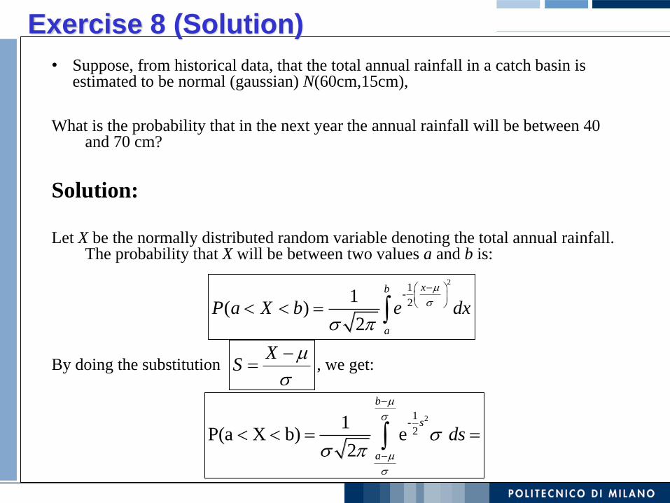
Exercise 8 (Solution)
• Suppose, from historical data, that the total annual rainfall in a catch basin is estimated to be normal (gaussian) N(60cm,15cm),
What is the probability that in the next year the annual rainfall will be between 40 and 70 cm?
Solution:
Let X be the normally distributed random variable denoting the total annual rainfall. The probability that X will be between two values a and b is:
By doing the substitution , we get:
21
-21
( )2
xb
a
P a X b e dx
XS
21-2
1P(a X b) e
2
b
s
a
ds
Exercise 8: Solution
21-2
1P(a X b) e
2
b
s
a
b ads
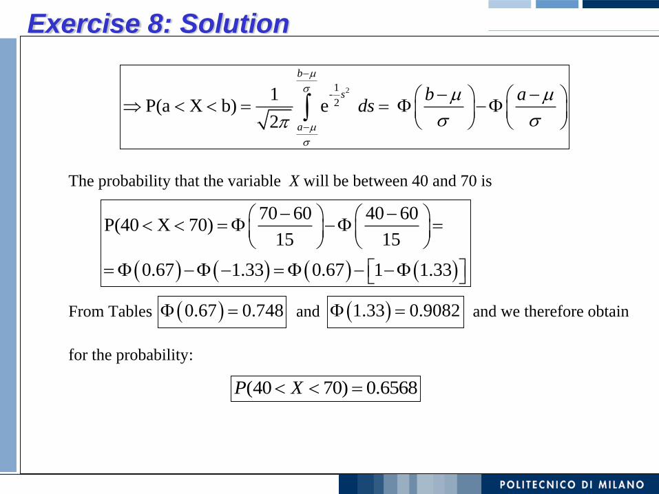
The probability that the variable X will be between 40 and 70 is
From Tables and and we therefore obtain
for the probability:
70 60 40 60P(40 X 70)
15 15
0.67 1.33 0.67 1 1.33
0.67 0.748 1.33 0.9082
(40 70) 0.6568P X
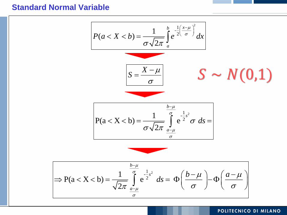
Standard Normal Variable
21
-21
( )2
xb
a
P a X b e dx
XS
21-2
1P(a X b) e
2
b
s
a
ds
21-2
1P(a X b) e
2
b
s
a
b ads
𝑆 ∼ 𝑁(0,1)
Central limit theorem
• For any sequence of n independent random variable Xi, their sum
𝑋 = σ𝑖=1𝑛 𝑋
𝑖is a random variable which, for large n, tends to be
distributed as a normal distribution

Piero Baraldi
Other Properties of Normal Variables
If 𝑋𝑖 are independent, identically distributed random variables with mean 𝜇 and finite variance given by 𝜎2
If 𝑋𝑖 are independent normal random variables with mean 𝜇i and finite variance given by 𝜎i
2, and 𝑏𝑖𝜖ℛ are constants
𝑄𝑛 =
𝑖=1
𝑛
𝑏𝑖𝑋𝑖 → 𝑁
𝑖=1
𝑛
𝑏𝑖𝜇𝑖 ,
𝑖=1
𝑛
𝑏𝑖2 𝜎2
𝑆𝑛=σ𝑖=0𝑛 𝑋𝑖
𝑛→ N(𝜇,
𝜎2
𝑛)
Exercise 9
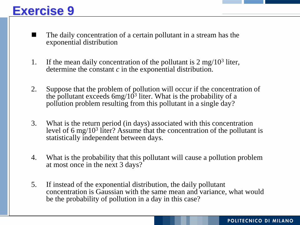
The daily concentration of a certain pollutant in a stream has the exponential distribution
1. If the mean daily concentration of the pollutant is 2 mg/103 liter, determine the constant c in the exponential distribution.
2. Suppose that the problem of pollution will occur if the concentration of the pollutant exceeds 6mg/103 liter. What is the probability of a pollution problem resulting from this pollutant in a single day?
3. What is the return period (in days) associated with this concentration level of 6 mg/103 liter? Assume that the concentration of the pollutant is statistically independent between days.
4. What is the probability that this pollutant will cause a pollution problem at most once in the next 3 days?
5. If instead of the exponential distribution, the daily pollutant concentration is Gaussian with the same mean and variance, what would be the probability of pollution in a day in this case?
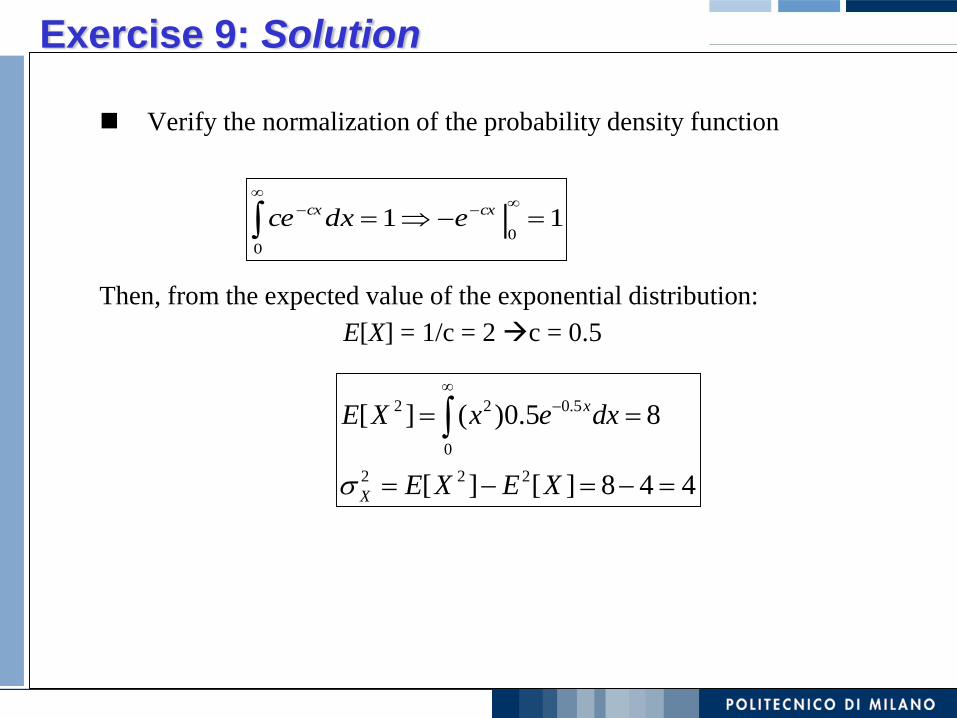
Exercise 9: Solution
Verify the normalization of the probability density function
Then, from the expected value of the exponential distribution:
E[X] = 1/c = 2 c = 0.5
00
11 |cxcx edxce
2 2 0.5
0
2 2 2
[ ] ( )0.5 8
[ ] [ ] 8 4 4
x
X
E X x e dx
E X E X
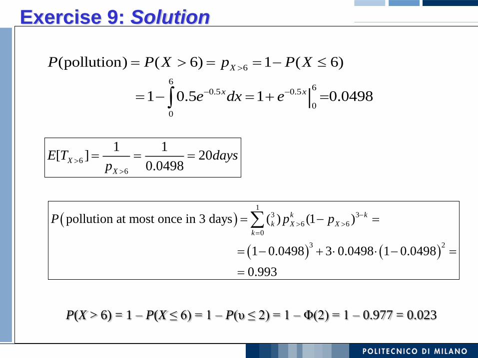
6
66
0.5 0.5
00
(pollution) ( 6) 1 ( 6)
1 0.5 1 0.0498|
X
x x
P P X p P X
e dx e
6
6
1 1[ ] 20
0.0498X
X
E T daysp
13 3
6 6
0
3 2
pollution at most once in 3 days ( ) (1 )
1 0.0498 3 0.0498 1 0.0498
k k
k X X
k
P p p
0.993
P(X > 6) = 1 – P(X ≤ 6) = 1 – P(υ ≤ 2) = 1 – Φ(2) = 1 – 0.977 = 0.023
Exercise 9: Solution
Piero Baraldi
Objectives of These Lectures
What is a random variable?
What is a probability density function (pdf)?
What is a cumulative distribution function (CDF)?
What is the hazard function and its relationship with the pdf and CDF?
The bath-tub curve
Binomial, Geometric and Poisson Distribution
Exponential Distribution and its memorylessproperty
Weibull Distribution
Gaussian Distribution and the central limit theorem
Piero Baraldi
Lecture 1,2,3,4: Where to study?
Slides
Red book (‘An introduction to the basics or reliability and risk analysis’, E. Zio):
4.1, 4.2,4.3 (no 4.3.4),4.4,4.5,4.6,
Exercises on Green Book (‘basics of reliability and risk analysis – Workout Problems and Solutions, E. Zio, P. Baraldi, F. Cadini)
All problems in Chapter 4
If you are interested in probabilistic approaches for treating uncertainty, you can refer to:
“Uncertainty in Risk Assessment – The Representation and Treatment of Uncertainties by
Probabilistic and Non-Probabilistic Methods”
Chapter 2
THE END (probably)
Thank you for the attention!!!!
Univariate continuous probability distributions:
1) exponential distribution
2) Weibull distribution
3) Normal distribution
4) Lognormal distribution
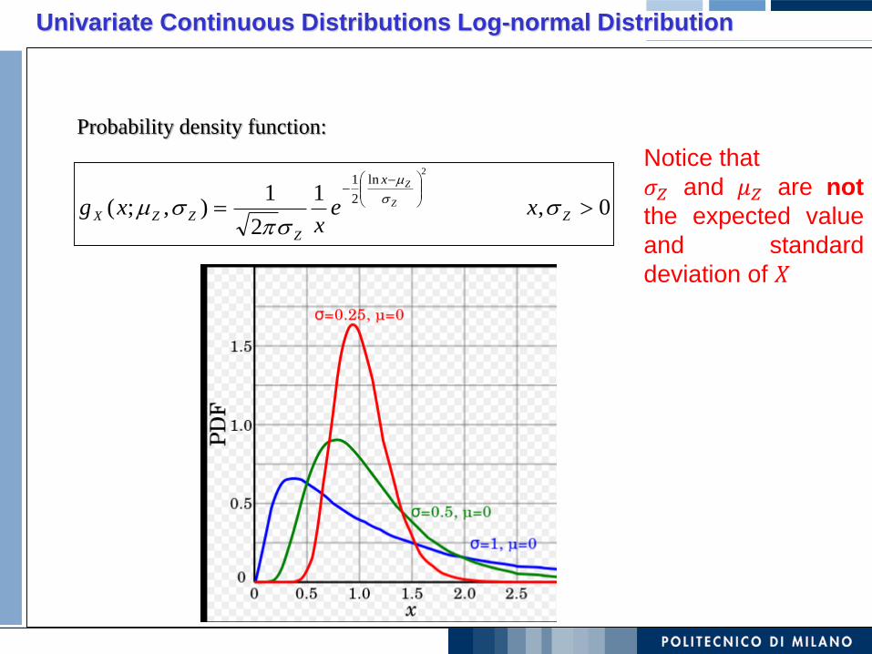
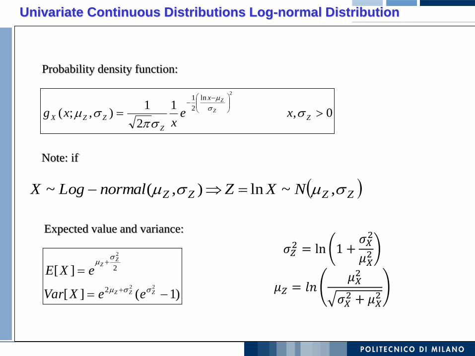
Univariate Continuous Distributions Log-normal Distribution
Probability density function:
0,1
2
1),;(
2ln
2
1
Z
x
Z
ZZX xex
xg Z
Z
Notice that
𝜎𝑍 and 𝜇𝑍 are not
the expected value
and standard
deviation of 𝑋
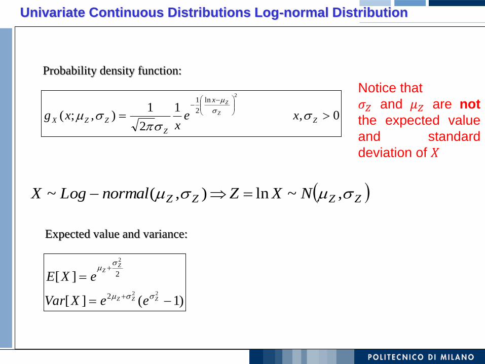
Univariate Continuous Distributions Log-normal Distribution
Probability density function:
Expected value and variance:
)1(][
][22
2
2
2
ZZZ
ZZ
eeXVar
eXE
0,1
2
1),;(
2ln
2
1
Z
x
Z
ZZX xex
xg Z
Z
ZZZZ NXZnormalLogX ,~ln),(~
Notice that
𝜎𝑍 and 𝜇𝑍 are not
the expected value
and standard
deviation of 𝑋
Univariate Continuous Distributions Log-normal Distribution
Probability density function:
Expected value and variance:
)1(][
][22
2
2
2
ZZZ
ZZ
eeXVar
eXE
0,1
2
1),;(
2ln
2
1
Z
x
Z
ZZX xex
xg Z
Z
ZZZZ NXZnormalLogX ,~ln),(~
Note: if
𝜎𝑍2 = ln 1 +
𝜎𝑋2
𝜇𝑋2
𝜇𝑍 = 𝑙𝑛𝜇𝑋2
𝜎𝑋2 + 𝜇𝑋
2
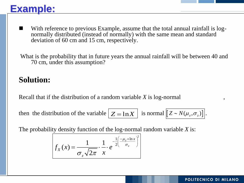
Example:
With reference to previous Example, assume that the total annual rainfall is log-normally distributed (instead of normally) with the same mean and standard deviation of 60 cm and 15 cm, respectively.
What is the probability that in future years the annual rainfall will be between 40 and 70 cm, under this assumption?
Solution:
Recall that if the distribution of a random variable X is log-normal ,
then the distribution of the variable is normal .
The probability density function of the log-normal random variable X is:
( , )z zZ N
2ln1
21 1( )
2
z
z
x
X
z
f x ex
XZ ln
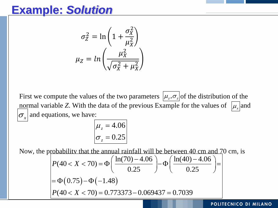
Example: Solution
First we compute the values of the two parameters of the distribution of the
normal variable Z. With the data of the previous Example for the values of and
and equations, we have:
Now, the probability that the annual rainfall will be between 40 cm and 70 cm, is
,z z
4.06
0.25
z
z
ln(70) 4.06 ln(40) 4.06(40 70)
0.25 0.25
0.75 1.48
(40 70) 0.773373 0.069437 0.7039
P X
P X
x
x
𝜎𝑍2 = ln 1 +
𝜎𝑋2
𝜇𝑋2
𝜇𝑍 = 𝑙𝑛𝜇𝑋2
𝜎𝑋2 + 𝜇𝑋
2


