Probability and Statistics Notes - faculty.tarleton.edu Chapter6.pdfProbability and Statistics Notes...

Probability and Statistics NotesChapter Six

Jesse Crawford

Department of MathematicsTarleton State University

Spring 2011

(Tarleton State University) Chapter Six Notes Spring 2011 1 / 45

Outline

1 Section 6.1: Point Estimation

2 Section 6.2 Confidence Intervals for Means

3 Section 6.3: Confidence Intervals for the Difference of Two Means

4 Section 6.4: Confidence Intervals for Variances

5 Section 6.5: Confidence Intervals for Proportions

6 Section 6.6: Sample Size


Statistical Models

Definition (Informal)A statistical model is a mathematical frameworkused to model random variables,where the probability distribution of the variables is not completelyknown.Often, the random variables represent a random samplefrom some population, where

I the parametric form of the population distribution is known, butI the actual values of the parameters are not.


Important Components of a Statistical ModelRandom variables X1, . . . ,Xn, which represent a sample fromsome population.A p.d.f./p.m.f. f (x ; θ), representing the population distribution.The unknown parameter θ, a number related to the populationdistribution whose value is not known.The parameter space, Ω, consisting of all possible values of θ.


ExampleIn a large city, the proportion of voters who approve of the mayoris unknown.A random sample X1, . . . ,Xn is taken from this city, whereXi = 1 if the i th voter approves, and Xi = 0 otherwise.

1 What p.d.f./p.m.f. should be used to model the population?2 What type of distribution is this?3 What is the unknown parameter, and what does it represent?4 What is the parameter space?5 Suppose 52% of the sample approves of the mayor. What would

be the best estimate for p?


The Likelihood Function

We can compactly summarize the assumptions of our statisticalmodel as

I X1, . . . ,Xn are IID,I with common distribution f (x ; θ), where θ ∈ Ω.

Therefore, the joint p.d.f./p.m.f. of X1, . . . ,Xn is

L(θ) = L(θ, x1, . . . , xn) = f (x1; θ) · · · f (xn; θ).

This function is called the likelihood function.The log-likelihood is

l(θ) = ln[L(θ)].

Intuitively, L(θ, x1, . . . , xn) is the likelihood of observingX1 = x1, . . . ,Xn = xn when the true value of the parameter is θ.


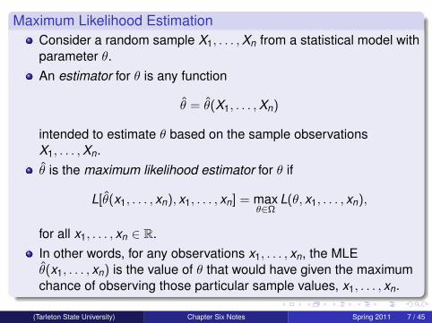
Maximum Likelihood EstimationConsider a random sample X1, . . . ,Xn from a statistical model withparameter θ.An estimator for θ is any function

θ = θ(X1, . . . ,Xn)

intended to estimate θ based on the sample observationsX1, . . . ,Xn.θ is the maximum likelihood estimator for θ if

L[θ(x1, . . . , xn), x1, . . . , xn] = maxθ∈Ω

L(θ, x1, . . . , xn),

for all x1, . . . , xn ∈ R.In other words, for any observations x1, . . . , xn, the MLEθ(x1, . . . , xn) is the value of θ that would have given the maximumchance of observing those particular sample values, x1, . . . , xn.


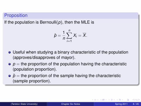
PropositionIf the population is Bernoulli(p), then the MLE is

p =1n

n∑i=1

Xi = X .

Useful when studying a binary characteristic of the population(approves/disapproves of mayor).p = the proportion of the population having the characteristic(population proportion).p = the proportion of the sample having the characteristic(sample proportion).


ExampleA company receives phone calls according to a Poisson process.Let X1, . . . ,Xn be n waiting times between successive phone calls.

1 What p.d.f./p.m.f. should be used to model the population?2 What type of distribution is this?3 What is the unknown parameter, and what does it represent?4 What is the parameter space?5 What is the MLE for θ?


ExampleIn a laboratory, mice have weights that are normally distributed.Let X1, . . . ,Xn be a random sample of n mice.

1 What p.d.f./p.m.f. should be used to model the population?2 What type of distribution is this?3 What is the unknown parameter, and what does it represent?4 What is the parameter space?5 What is the MLE for (µ, σ2)?


Unbiasedness

DefinitionLet θ be an estimator for a parameter θ.If E(θ) = θ, then θ is called unbiased. Otherwise, it is biased.


Multiple Regression

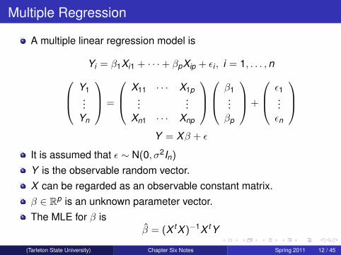
A multiple linear regression model is

Yi = β1Xi1 + · · ·+ βpXip + εi , i = 1, . . . ,n Y1...

Yn

=

X11 · · · X1p...

...Xn1 · · · Xnp

β1

...βp

+

ε1...εn

Y = Xβ + ε

It is assumed that ε ∼ N(0, σ2In)

Y is the observable random vector.X can be regarded as an observable constant matrix.β ∈ Rp is an unknown parameter vector.The MLE for β is

β = (X tX )−1X tY


Method of MomentsAnother method for estimating parameters is the method ofmoments.Suppose the model has r parameters θ1, . . . , θr .Equate the first r moments of the distribution to the first rmoments of the sample, and solve for the parameters to findestimates for them.

E(X ) =1n

n∑i=1

Xi

E(X 2) =1n

n∑i=1

X 2i

...

E(X r ) =1n

n∑i=1

X ri


Outline








Normal Population with Known Variance

Confidence Interval for µ whenPopulation is N(µ, σ2), andσ is known.

ExampleConsider math SAT scores at a university, and assumethey are normally distributed,the mean is unknown, andthe standard deviation is known to be 100.A random sample of size 200 is taken, andthe sample mean is 517.Estimate the average math SAT score at this university.Find a 95% confidence interval for the average math SAT score atthe university.


Normal Population with Known Variance

Proposition

If the population is N(µ, σ2), andthe population variance σ2 is known, then

P[X − zα/2

σ√n≤ µ ≤ X + zα/2

σ√n

]= 1− α.

A 1− α confidence interval for µ is[X − zα/2

σ√n,X + zα/2

σ√n

], or equivalently,

X ± zα/2σ√n.

The parameter µ is fixed.The confidence interval is random.


Normal Population with Unknown Variance

Confidence Interval for µ whenPopulation is N(µ, σ2), andσ is unknown.

ExampleConsider verbal SAT scores at a university, and assumethey are normally distributed,with unknown mean and standard deviation.A random sample of size 25 is taken,the sample mean is 561,and the sample standard deviation is 124.Estimate the average verbal SAT score at this university.Find a 95% confidence interval for the average verbal SAT scoreat the university.


Normal Population with Unknown Variance

Proposition

If the population is N(µ, σ2), andthe population variance σ2 is unknown, then

P[X − tα/2(n − 1)

s√n≤ µ ≤ X + tα/2(n − 1)

s√n

]= 1− α.

A 1− α confidence interval for µ is[X − tα/2(n − 1)

s√n,X + tα/2(n − 1)

s√n

],

or equivalently,X ± tα/2(n − 1)

s√n.


Large Sample Sizes

Recall that for values of n > 31,

t(n − 1) ≈ N(0,1), so

tα/2(n − 1) ≈ zα/2.

ExampleGas mileages of a certain type of vehicle are normally distributed.Gas mileage measurements are made on 100 vehicles, resultinginX = 33.5 and s = 5.68.Find a 90% confidence interval for the average gas mileage of allsuch vehicles.


Approximations for Non-normal Populations

ExampleA sample of 200 mice were exposed to a stimulus,and response times were measured, resulting ina mean response time of 1.12 seconds,and a standard deviation of 0.53 seconds.Find a 99% confidence interval for the mean response time in thepopulation.


Approximations for Non-normal Populations

PropositionFor non-normal populations,an approximate 1− α confidence interval for µ is

X ± tα/2(n − 1)s√n,

assuming that one of the following conditions holds:I n ≥ 30, orI the population distribution does not depart too far from normality

(for example, the approximation should be good for a symmetric,unimodal, continuous population distribution).


One-sided Confidence Intervals

Interested in a lower bound for µ.Use the one-sided 1− α confidence interval[

X − tα(n − 1)s√n,∞).

(Assuming appropriate conditions are met. Use zα instead whereappropriate.)


ExamplePipes manufactured by a company must have a mean strength ≥2400 lb/ft.In a sample of 150 pipes,the mean strength was 2437 lb/ft,and the standard deviation was 129 lb/ft.Find the relevant one-sided 99% confidence interval for the meanpipe strength.Does it appear that the pipes in the population exceed thestrength requirement?


One-sided Confidence Intervals

Interested in an upper bound for µ.Use the one-sided 1− α confidence interval(

−∞,X + tα(n − 1)s√n

].

(Assuming appropriate conditions are met. Use zα instead whereappropriate.)


ExampleMean emissions from car engines are required to be ≤ 20 ppm ofcarbon.The emissions statistics for a sample of 20 engines werex = 19.78 and s = 1.84.Find the relevant one-sided 99% confidence interval for theemissions levels.Does it appear that the engines in the population meet theemissions standards?


Outline








Normal Populations with Known Variances

Suppose X1, . . . ,Xn and Y1, . . . ,Ym are independent samplesfrom two normal distributions N(µX , σ

2X ) and N(µY , σ

2Y ),

where the variances σ2X and σ2

Y are known.A 1− α confidence interval for µX − µY is

X − Y ± zα/2

√σ2

X/n + σ2Y/m.


Normal Populations with Common Unknown Variance

Suppose X1, . . . ,Xn and Y1, . . . ,Ym are independent samplesfrom two normal distributions N(µX , σ

2) and N(µY , σ2),

with common, unknown variance σ2.A 1− α confidence interval for µX − µY is

X − Y ± tα/2(n + m − 2)Sp

√1n

+1m,

where Sp is the pooled estimator of σ,

Sp =

√(n − 1)S2

X + (m − 1)S2Y

n + m − 2.


Large Samples

Suppose X1, . . . ,Xn and Y1, . . . ,Ym are large independentsamples (n,m ≥ 30)from two distributions with means µX and µY .A 1− α confidence interval for µX − µY is

X − Y ± zα/2

√S2

X/n + S2Y/m.

We are not assuming normality, common variance, or knownvariance


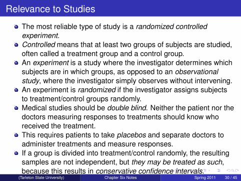
Relevance to Studies

The most reliable type of study is a randomized controlledexperiment.Controlled means that at least two groups of subjects are studied,often called a treatment group and a control group.An experiment is a study where the investigator determines whichsubjects are in which groups, as opposed to an observationalstudy, where the investigator simply observes without intervening.An experiment is randomized if the investigator assigns subjectsto treatment/control groups randomly.Medical studies should be double blind. Neither the patient nor thedoctors measuring responses to treatments should know whoreceived the treatment.This requires patients to take placebos and separate doctors toadminister treatments and measure responses.If a group is divided into treatment/control randomly, the resultingsamples are not independent, but they may be treated as such,because this results in conservative confidence intervals.


Paired Observations

Suppose (X1,Y1), . . . , (Xn,Yn) are n pairs of measurementswhere E(Xi) = µX and E(Yi) = µY , for i = 1, . . . ,n.Let Di = Xi − Yi , for i = 1, . . . ,n.Assuming the populations are normally distributed or thesample size is large (n ≥ 30),a 1− α confidence interval for µX − µY is

D ± tα/2(n − 1)SD√

n.


Outline








CI for Variance of a Normal Population

Suppose X1, . . . ,Xn is a random sample from N(µ, σ2),and let a and b be constants such that

P[a ≤ χ2(n − 1) ≤ b] = 1− α,

i.e., a = χ21−α/2(n − 1) and b = χ2

α/2(n − 1).

Then a 1− α confidence interval for σ2 is[(n − 1)S2

b,

(n − 1)S2

a

].


Outline








Mathematical Framework for Proportions

Consider a population whose subjects have some binarycharacteristic (approves of mayor or doesn’t).The proportion of the population with the characteristic is p, thepopulation proportion.Mathematically, the population is just Bernoulli(p).Let X1, . . . ,Xn be a sample from this population, and letY =

∑ni=1 Xi .

Then Y ∼ Binomial(n,p).The MLE for the population proportion p is the sample proportion

p =Yn

=

∑ni=1 Xi

n= X .


Also note that the population mean and variance are

µ = p and σ2 = p(1− p).

In particular, a good estimator for σ2 is

σ2 = p(1− p) ≈ S2.

Therefore, as long as the CLT applies (np ≥ 5 and n(1−p) ≥ 5),all inferences for a population proportion are the same as thosefor a population mean, using the following dictionary:

Means Proportionsµ pX pS

√p(1− p)


Confidence Intervals for Populations Proportions

If np ≥ 5 and n(1− p) ≥ 5, a 1− α confidence interval for a populationproportion is

p ± zα/2

√p(1− p)

n.

If either np or n(1− p) is less than 5, replace p with

p =Y + 2n + 4

.


Difference in Population Proportions

Consider independent samples of sizes n1 and n2

from two populations with proportions p1 and p2, respectively.A 1− α confidence interval for p1 − p2 is

p1 − p2 ± zα/2

√p1(1− p1)

n1+

p2(1− p2)

n2.


Outline








Sample Size for Population Mean

ExampleSuppose you want to estimate the gas mileage of a certain type ofcar.You want a 95% confidence level that is within 2 mpg of the truegas mileage.Based on a preliminary study, the standard deviation of the gasmileages is about 5.68 mpg.What sample size is required to obtain the desired confidenceinterval?


Letting ε denote the desired margin of error, we have

ε = zα/2s√n,

so the necessary sample size is

n =z2α/2s2

ε2 .


Sample Size for Population Proportion

ExampleSuppose the unemployment rate has been near 8% recently.We wish to estimate the unemployment rate within 0.001 with a99% confidence level.What sample size is required?

n =z2α/2p(1− p)

ε2 .


Population Proportion with No Preliminary Estimate

ExamplePolitician is considering running for governor.Wants to estimate her approval rating within 0.03 with 95%confidence.What sample size is required?

n =z2α/2

4ε2 .


Finite Population Correction Factor

All of our results so far have assumed an infinite population.Generally, if the sample size is ≤ 5% of the population size, thepopulation can be regarded as infinite.For finite populations, the variance of the estimators X and p ismultiplied by the finite population correction factor,

N − nN − 1

,

where N = population size, and n = sample size.


Confidence Intervals for Finite Populations

X ± zα/2s√n

√N − nN − 1

p ± zα/2

√p(1− p)

n

(N − nN − 1

).


ExampleConsider a population of 750 college algebra students.Suppose we want to estimate the proportion p of these studentswho met certain performance standards on their final exams.We would like to estimate p within 0.05 with 95% confidence.What sample size is required?


Probability and Statistics Notes - faculty.tarleton.edu Chapter6.pdfProbability and Statistics Notes...

Documents

Transcript of Probability and Statistics Notes - faculty.tarleton.edu Chapter6.pdfProbability and Statistics Notes...