Probability distribution for monthly precipitation data in India

Anumandla Sukrutha1, Sristi Ram Dyuthi2, and Shantanu Desai3

1Dept. of Electrical Engineering, IIT Hyderabad, Kandi, Telangana 502285, India

Email:ee14btech11002@iith.ac.in2Dept. of Electrical Engineering, IIT Hyderabad, Kandi, Telangana 502285, India

Email:ee14btech11031@iith.ac.in3Dept. of Physics, IIT Hyderabad, Kandi, Telangana 502285, India Email:shantanud@iith.ac.in

ABSTRACT

We carry out a study of the statistical distribution of rainfall precipitation data for various cites in

India, motivated by similarwork done inGhosh et al. 2016, which studied the probability distribution

of rainfall in multiple cities in Bangladesh. We have determined the best-fit probability distribution

for the monthly precipitation data spanning 100 years of data from 1901 to 2002, for multiple

stations located all over India, such as Gandhinagar, Guntur, Hyderabad, Jaipur, Kohima, Kurnool,

and Patna. To fit the observed data, we considered the Fisher, Gamma, Gumbel, Inverse Gaussian,

Normal, Weibull, Student-t, Beta, and Generalized Extreme Value distributions. The efficacy of

the fits for these distributions are evaluated using four empirical non-parametric goodness-of-fit

tests namely Kolmogorov-Smirnov (KS), Anderson-Darling (AD), Chi-Square, Akaike information

criterion(AIC) and Bayesian Information criterion (BIC). Finally, the best-fit distribution using each

of these tests are reported for the various cities.

INTRODUCTION

Establishing a probability distribution that provides a good fit to the monthly average pre-

cipitation across years has long been a topic of interest in the fields of hydrology, meteorology,

1

arX

iv:1

708.

0314

4v1

[st

at.A

P] 1

0 A

ug 2

017

agriculture, and others. The knowledge of precipitation at a given location is an important pre-

requisite for agricultural planning and management. Rainfall is the main source of precipitation.

Studies of precipitation provide us knowledge about rainfall. For rain-fed agriculture, rainfall is the

single most important agro-meteorological variable influencing crop production. In the absence

of reliable, physically based seasonal forecasts, crop management decisions and planning have to

rely on statistical assessment based on the analysis of historical precipitation records. Therefore,

probability distribution of rainfall data in a variety of countries such as New Zealand, Japan, South

Korea have been studied (Ghosh et al. 2016). Hirose 1994 found that the daily rainfall distribution

in Japan is best fit by a Weibull distribution. Nadarajah and Choi 2007 found that Gumbel distri-

bution provides the most reasonable fit to the data in South Korea. Most recently, Ghosh et al.

2016 fitted the rainfall data from 5 stations in Bangladesh to six probability distributions and used

three different tests : Kolmogorov-Smirnoff ( test, Anderson-Darling test, and chi-square test. They

found that the extreme value distribution provides the best fit to the Chittagong monthly rainfall

data during the rainy season, whereas for Dhaka, the gamma distribution provides a better fit.

The main objective of the current study is to determine the best fit probability distribution

for the monthly average precipitation data of selected stations in India. The best fit probability

distribution was evaluated on the basis of several goodness of fit tests. We replicate more or less

the same procedure as in Ghosh et al. 2016 (modulo two additional goodness of fit tests using

Akaike and Bayesian Information Criterion, not carried out in therein, for these Indian stations.

The precipitation-based information generated by this study is expected to be of considerable

agronomic importance for the efficient planning and management of rain fed cotton based cropping

system. Apart from agriculture point of view, the current study also finds its importance in

the estimation of extreme precipitation for design purposes, assessment of rarity of observed

precipitation, comparison of methods to estimate design precipitation which is useful for planners.

Previous recent studies of rainfall distribution of Indian stations can be found in (Sharma and Singh

2010; Deka et al. 2009).

2

DATASET

The dataset employed here for our study spans a 100 year period from 1901 to 2002, and is

collected by the Indian Meteorological Department and can be downloaded from http://www.

indiawaterportal.org/met_data/. The stations used for this study are Gandhinagar, Guntur,

Hyderabad, Jaipur, Kohima, Kurnool, Patna. We briefly list the stations below.

Gandhinagar Gandhinagar is the Capital of Gujarat and located in the western part of India. Its

geographical coordinates are 23.223 deg N, 72.650 deg E. It covers a total area of 177 sq.km. It is

located at an elevation of 81 m. The average annual rainfall is around 803.4 mm.

Guntur Guntur is the Capital of Andhra Pradesh, located in the southern part of India. Its

geographical Coordinates are 16.3008 deg N, 80.4428 deg E. It covers a total area of 168.41 square

km. It is located at an elevation of 30 m. The average annual rainfall is around 906 mm.

Hyderabad Hyderabad is the Capital of Telangana, also in the southern part of India. Its

geographical Coordinates are 17.37 deg N, 78.48 deg E. It covers a total area of 650 sq.km. It is

located at an elevation of 505 m. The average annual rainfall is around 828 mm.

Jaipur Jaipur is the capital and the largest city of the Indian city of Rajasthan, in the western part

of India. Its geographical Coordinates are 26.9 deg N, 75.8 deg E. It covers a total area of 484.64

sq.km. It is at an elevation of 431 m. The average annual rainfall is around 635.4 mm.

Kohima Kohima is the hilly Capital of India’s north eastern border state of Nagaland. Its

geographical Coordinates are 25.67 deg N, 94.12 deg E. It covers a total area of 20 sq.km. It is at

an elevation of 1261 m. The average annual rainfall is around 1831.3 mm.

Kurnool Kurnool is a city, former princely state and the headquarters of Kurnool district in the

Indian state of Andhra Pradesh. Its geographical Coordinates are 15.83 deg N, 78.05 deg E. It

3

covers a total area of 65.91 sq.km. It is at an elevation of 274 m. The average annual rainfall is

around 737.2 mm.

Patna Patna is the capital and largest city of the state of Bihar in India. Its geographical

coordinates are 25.6 deg N, 85.1 deg E. It covers a total area of 99.45 sq.km. It is at an elevation of

53 m. The average annual rainfall is around 1019.4 mm.

METHODOLOGY

The probability distributions considered for fitting the rainfall data are gamma, Fisher, Inverse

Gaussian, Normal, Student−t, LogNormal, Generalized Extreme value, Weibull, and Beta. The

mathematical expressions for the probability density functions of these distributions can be found

in Table 1. The distribution of rainfall for all the seven stations along with the best fit distributions

is shown in Figs.1-7.

Model Comparison tests

We use multiple model comparison methods to carry out hypothesis testing and select the best

distribution for the precipitation data. The test is performed in order to select among the following

hypotheses:

H0 : The amount of monthly precipitation data follows a specified distribution.

H1 : The amount of monthly precipitation data does not follow the specified distribution. In

other words, H1 is the complement of H0.

The goodness of fit tests conducted herein include non-parametric distribution-free tests such

as Kolmogorov−Smirnov Test, Anderson-Darling Test, Chi−square test and information-criterion

tests such as Akaike and Bayesian Information Criterion. For each of the probability distributions,

we find the best-fit parameters for each of the stations using least-squares fitting and then carry out

the different model comparison tests discussed below.

Kolmogorov-Smirnov Test

The Kolmogorov-Smirnov (K-S) test (Vetterling et al. 1992) is a non-parametric test used to

decide if a sample comes from a population with a specific distribution. The K-S test compares the

4

empirical distribution function (ECDF) of two samples. Given N ordered data points y1, y2, ..., yN,

the ECDF is defined as

EN = n(i)/N, (1)

where n(i) indicates the total number of points less than yi after sorting the yi in increasing order.

This is a step function that increases by 1/N for each sorted data point.

The K-S test is based on the maximum distance between the empirical distribution function and

the normal cumulative distributive function. An attractive feature of this test is that the distribution

of the K-S test statistic itself does not depend on the statistics of the parent distribution from which

the samples are drawn. Some limitations are that it applies only to continuous distributions and

tends to be more sensitive near the center of the distribution than at the tails.

The Kolmogorov-Smirnov test statistic is defined as:

D = max16i6N

(F(yi) −i − 1

N,

iN− F(yi)), (2)

where F is the cumulative distribution function of the samples (or a probability distribution function)

being tested. If the probability that a given value of D is very small (less than a certain critical

value, which can be obtained from tables) we can reject the null hypothesis that the two samples

are drawn from the same underlying distributions at a given confidence level.

Anderson-Darling Test

The Anderson-Darling test (VanderPlas et al. 2012) is another test (similar to K-S test), which

can evaluate whether a sample of data came from a population with a specific distribution. It is a

modification of the K-S test and gives more weight to the tails compared to the K-S test. The K-S

test is distribution free in the sense that the critical values do not depend on the specific distribution

being tested. The Anderson-Darling test makes use of the specific distribution in calculating critical

values. This has the advantage of allowing a more sensitive test. However, one disadvantage is that

the critical values must be calculated separately for each distribution. The Anderson-Darling test

5

statistic is defined as follows (VanderPlas et al. 2012):

A2 = −N −N∑

i=1

(2i − 1)N[log F(yi) + log(1 − F(yN+1−i))] (3)

F is the cumulative distribution function of the specified distribution. yi denote the sorted data.

The test is a one-sided test and the hypothesis that the data is sampled from a specific distribution

is rejected if the test statistic, A, is greater than the critical value. For a given distribution, the

Anderson-Darling statistic may be multiplied by a constant (depending on the sample size, n).

These constants have been tabulated by Stephens (Stephens 1974).

Chi-Square Test

The chi-square test (Vetterling et al. 1992) is used to test if a sample of data is obtained from a

population with a specific distribution. An attractive feature of the chi-square goodness-of-fit test

is that it can be applied to any univariate distribution for which you can calculate the cumulative

distribution function. The chi-square goodness-of-fit test is applied to binned data. The value of

the chi-square test statistic is dependent on how the data is binned. Another disadvantage of the chi-

square test is that it requires a sufficiently large sample size in order for the chi-square approximation

to be valid. The chi-square goodness-of-fit test can be applied to discrete distributions such as the

binomial and the Poisson distributions. The Kolmogorov-Smirnov and Anderson-Darling tests are

restricted to continuous distributions. For the chi-square goodness-of-fit computation, the data are

divided into k bins and the test statistic is defined as follows:

χ2 =k∑

i=1

(Oi − Ei)2Ei

, (4)

whereOi is the observed frequency for bin i and Ei is the expected frequency for bin i. The expected

frequency is calculated by

Ei = N(F(Yu) − F(Yl)), (5)

6

where F is the cumulative distribution function for the distribution being tested, Yu is the upper

limit for class i, Yl is the lower limit for class i, and N is the sample size.

This test is sensitive to the choice of bins. There is no optimal choice for the bin width (since the

optimal bin width depends on the distribution). Most reasonable choices should produce similar,

but not identical results. For the chi-square approximation to be valid, the expected frequency of

events in each bin should be at least five. This test is not valid for small samples, and if some of the

counts are less than five, you may need to combine some bins in the tails. The test statistic follows,

approximately, a chi-square distribution with (k − c) degrees of freedom where k is the number of

non-empty cells and c is the number of estimated parameters (including location, scale, and shape

parameters) for the distribution + 1. Therefore, the hypothesis that the data are from a population

with the specified distribution is rejected if:

χ2 > χ1−α,k−c2, (6)

where χ1−α,k−c2 is the chi-square critical value with k − c degrees of freedom and significance level

α.

AIC and BIC

The Akaike Information Criterion (AIC) (Liddle 2004; Kulkarni and Desai 2017) is a way of

selecting a model from a set of models. It can be derived by an approximate minimization of the

Kullback-Leibler distance between the model and the truth. It is based on information theory, but a

heuristic way to think about it is as a criterion that seeks a model that has a good fit to the truth but

few parameters. It has been extensively used in Astrophysics for model comparison (Liddle 2007).

It is defined as (Kulkarni and Desai 2017):

AIC = −2(log(L)) + 2K (7)

where L is the likelihood which denotes the probability of the data given a model, and K is the

number of free parameters in the model. AIC scores are often shown as ∆AIC scores, or difference

7

between the best model (smallest AIC) and each model (so the best model has a ∆AIC of zero).

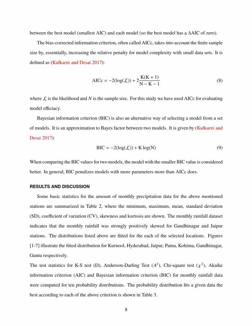
The bias-corrected information criterion, often called AICc, takes into account the finite sample

size by, essentially, increasing the relative penalty for model complexity with small data sets. It is

defined as (Kulkarni and Desai 2017):

AICc = −2(log(L)) + 2K(K + 1)N − K − 1

(8)

where L is the likelihood and N is the sample size. For this study we have used AICc for evaluating

model efficiacy.

Bayesian information criterion (BIC) is also an alternative way of selecting a model from a set

of models. It is an approximation to Bayes factor between two models. It is given by (Kulkarni and

Desai 2017):

BIC = −2(log(L)) + K log(N) (9)

When comparing the BIC values for twomodels, themodel with the smaller BIC value is considered

better. In general, BIC penalizes models with more parameters more than AICc does.

RESULTS AND DISCUSSION

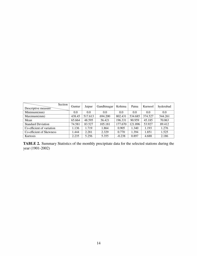
Some basic statistics for the amount of monthly precipitation data for the above mentioned

stations are summarized in Table 2, where the minimum, maximum, mean, standard deviation

(SD), coefficient of variation (CV), skewness and kurtosis are shown. The monthly rainfall dataset

indicates that the monthly rainfall was strongly positively skewed for Gandhinagar and Jaipur

stations. The distributions listed above are fitted for the each of the selected locations. Figures

[1-7] illustrate the fitted distribution for Kurnool, Hyderabad, Jaipur, Patna, Kohima, Gandhinagar,

Guntu respectively.

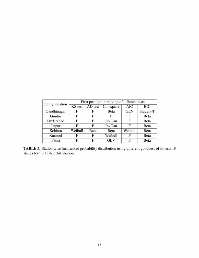
The test statistics for K-S test (D), Anderson-Darling Test (A2), Chi-square test (χ2), Akaike

information criterion (AIC) and Bayesian information criterion (BIC) for monthly rainfall data

were computed for ten probability distributions. The probability distribution fits a given data the

best according to each of the above criterion is shown in Table 3.

8

Our results from the various model comparison tests are as follows:

• Using K-S test (D), we find that the Fisher distribution provides a good fit to the monthly

precipitation data at Guntur, Jaipur, Gandhinagar, Patna, Kurnool and Hyderabad. For

Kohima, Weibull distribution provides good fit.

• Using Anderson-Darling Test (A2), it is observed that the Fisher distribution provides the

best distribution for all the cities except Kohima, for which the Beta distribution gives the

best fit.

• Using Chi-square test (χ2), it is observed that the Fisher distribution provides best distribu-

tion for Guntur. Beta distribution fits best for Gandhinagar, Kohima and Kurnool. Inverse

Gaussian distribution provides the best fit for Jaipur and Hyderabad and generalized extreme

value distribution provides good fit to the monthly precipitation data at Patna.

• UsingAkaike information criterion (AIC), it is observed that the Fisher distribution provides

best distribution for Guntur, Jaipur, Patna, Kurnool and Hyderabad. Generalized extreme

value distribution provides good fit for Gandhinagar andWeibull distribution provides good

fit for Kohima.

• Using Bayesian information criterion (BIC), it is observed that beta distribution provides

best distribution for all districts except Gandhinagar. Student-t distribution provides best fit

for Gandhinagar.

IMPLEMENTATION

We have used the python2.7 environment. In addition, Numpy, pandas, matplotlib, scipy

packages are used. Our codes to reproduce all these results can be found in https://drive.

google.com/drive/u/0/folders/0By2cFqNljWi_QkxOaXNHalI1aFk.

COMPARISON TO PREVIOUS RESULTS

We now briefly compare our results to two recent papers which studied probability distribution

of rainfall at various locations in India. Deka et al (Deka et al. 2009) used five distributions

Generalized Extreme Value, Generalized Logistic, Generalized Pareto, Lognormal and Pearson

9

distribution. The method they used is similar to the one which we followed. However, instead of

estimating the parameters using L-moments method they followed LQ-moment. For goodness of

fit, they didn’t use AIC, BIC, or χ2. Instead they used RRMSE, PPCC, RMAE. Their analysis was

applied to data from only the eastern states.

Sharma et al (Sharma and Singh 2010) did their analysis on the daily, weekly, monthly, seasonal,

and annual data for 37 years, whereas we did the same analysis on 100 years data. There goodness of

fit parameters are similar to ours but they did not use BIC for model comparison. The distributions

they selected are normal, lognormal (2P,3P), gamma (2P, 3P), generalized gamma (3P,4P), log-

gamma, weibull (2P,3P), pearson 5 (2P,3P), pearson 6 (3P, 4P), log-pearson 3, and generalized

extreme value. Their method of calculating best fit is bit different. Rankings are given to the

distributions based on the goodness of fit values and the top four distributions are selected. Random

numbers are generated and the four distributions. Then the residuals (Least-Squares) are calculated

for each distribution. The distribution having minimum sum of residuals was considered to be the

best-fit probability distribution for that particular data set.

CONCLUSION

We carried out a systematic study to identify the best fit probability distribution for the monthly

precipitation data at seven selected stations of India. The data showed that the monthly minimum

and maximum precipitation at any time at any station ranged from 0 to 802 mm, which obviously

indicates a large dynamic range. So identifying the best parametric distribution for the monthly

rainfall data could have a wide range of applications in agriculture, hydrology, engineering design,

and climate research. For each station, we fit the precipitation data to 10 distributions described

in Table 1. To determine the best fit among these distributions, we used five model comparison

tests, such as K-S test, Anderson-Darling test, chi-square test, Akaike and Bayesian Information

criterion. The results from these tests are summarized in Table 3. We find that no one distribution

can adequately describe the rainfall data for all the stations. Also, sometimes there is no consensus

between the different model comparison tests for the same data. According to K-S, Anderson-

Darling and AIC, the Fisher distribution is preferred for most of the cities. According to BIC, the

10

beta distribution best fits the data for all cities except Gandhinagar.

REFERENCES

Deka, S., Borah, M., and Kakaty, S. (2009). “Distributions of annual maximum rainfall series of

north-east india.” European Water, 27(28), 3–14.

Ghosh, S., Roy, M. K., and Biswas, S. C. (2016). “Determination of the best fit probability

distribution for monthly rainfall data in bangladesh.” American Journal of Mathematics and

Statistics, 6(4), 170–174.

Hirose, H. (1994). “Parameter estimation in the extreme-value distributions using the continuation

method.” Transactions of Information Processing Society of Japan, 35(9).

Kulkarni, S. and Desai, S. (2017). “Classification of gamma-ray burst durations using robust

model-comparison techniques.” Astrophysics and Space Science, 362(4), 70.

Liddle, A. R. (2004). “How many cosmological parameters.” Monthly Notices of the Royal Astro-

nomical Society, 351(3), L49–L53.

Liddle, A. R. (2007). “Information criteria for astrophysical model selection.” Monthly Notices of

the Royal Astronomical Society: Letters, 377(1), L74–L78.

Nadarajah, S. and Choi, D. (2007). “Maximum daily rainfall in south korea.” Journal of Earth

System Science, 116(4), 311–320.

Sharma, M. A. and Singh, J. B. (2010). “Use of probability distribution in rainfall analysis.” New

York Science Journal, 3(9), 40–49.

Stephens, M. A. (1974). “Edf statistics for goodness of fit and some comparisons.” Journal of the

American statistical Association, 69(347), 730–737.

VanderPlas, J., Connolly, A. J., Ivezić, Ž., and Gray, A. (2012). “Introduction to astroml: Machine

learning for astrophysics.” Intelligent Data Understanding (CIDU), 2012 Conference on, IEEE,

47–54.

Vetterling, W. T., Teukolsky, S. A., and Press, W. H. (1992). Numerical recipes: example book (C).

Press Syndicate of the University of Cambridge.

11

List of Tables

1 Probability density functions of different distributions used to fit the rainfall data

are listed in this table. The mathematical expressions for each of these can be found

in any statistics textbook. . . . . . . . . . . . . . . . . . . . . . . . . . . . . . . . 13

2 Summary Statistics of the monthly precipitate data for the selected stations during

the year (1901-2002) . . . . . . . . . . . . . . . . . . . . . . . . . . . . . . . . . 14

3 Station wise first ranked probability distribution using different goodness of fit tests.

F stands for the Fisher distribution. . . . . . . . . . . . . . . . . . . . . . . . . . . 15

12

Distribution Probability density functionNormal f (x) = 1√

2πσ2exp− (x−µ)

2

2σ2

Lognormal f (x) = 1x√

2πσ2exp− (ln x−µ)2

2σ2

Gamma f (x) = 1x√

2πσ2exp− (ln x−µ)2

2σ2

Inverse Gaussian f (x) = λ2πx3

0.5 exp −λ(x−µ)2

2µ2x

GEV f (x) = 1σ [1 − k x−µ

σ ]1/k−1exp[−(1 − k x−µσ )]

1/k

Gumbel f (x) = 1/β exp(−z + exp(−z))), z = x−µβ

Student-t f (x) = Γ( v+12 )√

vπΓ(v/2) (1 +x2

v )−v−1

2

Beta f (x) = xα−1(1−x)β−1

Γ(α)Γ(β)Γ(α+β)

Weibull f (x) = kλ (

xλ )k−1e−(

xλ )k

Fisher

√(d1x)

d1 dd22

(d1x+d2)d1+d2

xB( d12 ,

d22 )

TABLE 1. Probability density functions of different distributions used to fit the rainfall data arelisted in this table. The mathematical expressions for each of these can be found in any statisticstextbook.

13

hhhhhhhhhhhhhhhhhhDescriptive measureSection Guntur Jaipur Gandhinagar Kohima Patna Kurnool hyderabad

Minimum(mm) 0.0 0.0 0.0 0.0 0.0 0.0 0.0Maximum(mm) 438.45 517.613 694.200 802.431 534.685 374.527 544.261Mean 65.664 48.595 56.421 196.331 90.959 45.185 70.063Standard Deviation 74.581 83.527 105.181 177.670 121.896 53.927 89.412Co-efficient of variation 1.136 1.719 1.864 0.905 1.340 1.193 1.276Co-efficient of Skewness 1.444 2.281 2.329 0.770 1.394 1.851 1.525Kurtosis 2.235 5.256 5.355 -0.238 0.897 4.688 2.186

TABLE 2. Summary Statistics of the monthly precipitate data for the selected stations during theyear (1901-2002)

14

Study location First position in ranking of different testsKS test AD test Chi square AIC BIC

Gandhinagar F F Beta GEV Student-TGuntur F F F F Beta

Hyderabad F F InvGau F BetaJaipur F F InvGau F BetaKohima Weibull Beta Beta Weibull BetaKurnool F F Weibull F BetaPatna F F GEV F Beta

TABLE 3. Station wise first ranked probability distribution using different goodness of fit tests. Fstands for the Fisher distribution.

15

List of Figures

1 Distribution fit for monthly precipitate data at Kurnool. . . . . . . . . . . . . . . . 17

2 Distribution fit for monthly precipitate data at Hyderabad. . . . . . . . . . . . . . . 18

3 Distribution fit for monthly precipitate data at Jaipur. . . . . . . . . . . . . . . . . 19

4 Distribution fit for monthly precipitate data at Patna. . . . . . . . . . . . . . . . . . 20

5 Distribution fit for monthly precipitate data at Kohima. . . . . . . . . . . . . . . . 21

6 Distribution fit for montly precipitate data at Gandhinagar. . . . . . . . . . . . . . 22

7 Distribution fit for montly precipitate data at Guntur. . . . . . . . . . . . . . . . . 23

16

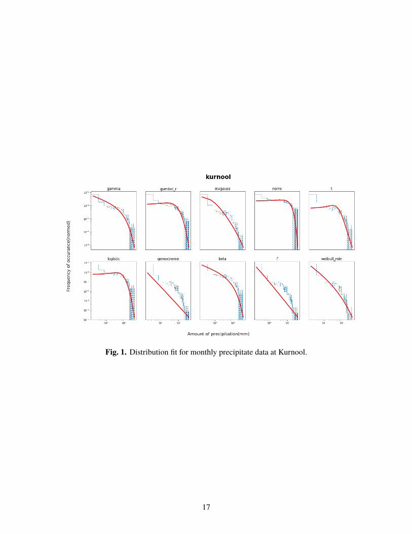
Fig. 1. Distribution fit for monthly precipitate data at Kurnool.

17

Fig. 2. Distribution fit for monthly precipitate data at Hyderabad.

18

Fig. 3. Distribution fit for monthly precipitate data at Jaipur.

19

Fig. 4. Distribution fit for monthly precipitate data at Patna.

20

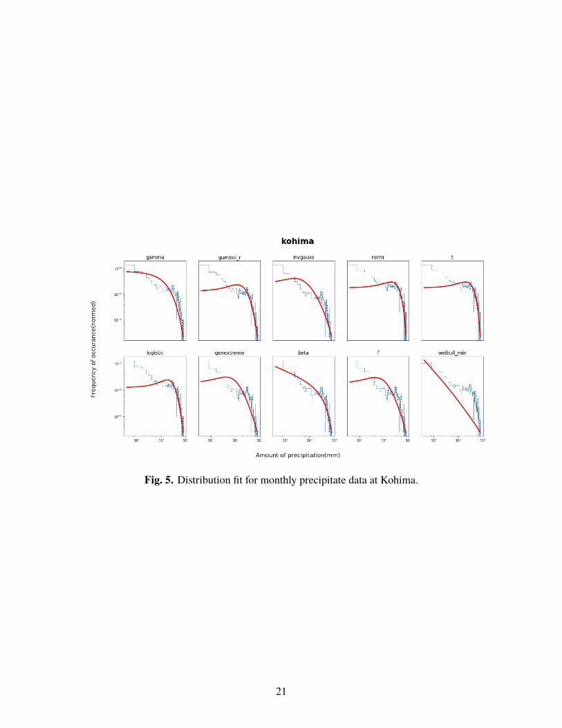
Fig. 5. Distribution fit for monthly precipitate data at Kohima.

21

Fig. 6. Distribution fit for montly precipitate data at Gandhinagar.

22

Fig. 7. Distribution fit for montly precipitate data at Guntur.

23