PROBABILISTIC MODELLING OF AIR POLLUTION FROM ROAD TRAFFIC

PROBABILISTIC MODELLING OF AIR POLLUTION FROM ROAD TRAFFIC

by

SAM-ERIK WALKER

THESIS

for the degree of

MASTER OF SCIENCE

(Master i Modellering og dataanalyse)

Faculty of Mathematics and Natural Sciences

University of Oslo

August 2010

Det matematisk-naturvitenskapelige fakultet

Universitetet i Oslo

1

ACKNOWLEDGEMENTS

First of all I would like to thank my supervisor Prof. Geir Olve Storvik at the Department of Mathematics, University of Oslo, for excellent guidance and for the many good advices that I’ve received during this work.

I also want to thank my many colleagues at the Norwegian Institute for Air Research (NILU) for their support and encouragement. In particular, I wish to thank former Director Elin Marie Dahlin and current Director Leonor Tarrasón for their special encouragement and support; Karl Idar Gjerstad for preparing emission data for the model runs; Dag Tønnesen for his efforts to define Bayesian prior distributions for one of the stochastic models; Terje Krognes for building a fast multi-core PC for which parts of the calculations have been run; and last but not least Bruce Rolstad Denby for financial support through our data assimilation SIP project.

I would also like to thank Dyre Dammann for his efficient efforts in preparing data and performing numerous calculations with the WORM model during his stay at NILU in July 2008 and June-July 2009, and John S. Irwin for many stimulating discussions about the WORM model development during his visit to NILU in November 2007.

At NILU, this work was funded by the Norwegian Research Council through the Strategic Institute Program (SIP) project “Development and use of ensemble based data assimilation methods in atmospheric chemistry modelling”.

3

TABLE OF CONTENTS

ABSTRACT...................................................................................................................... 5

1. INTRODUCTION ....................................................................................................... 7 1.1 Background ...................................................................................................... 7 1.2 Aim of the work ............................................................................................... 8 1.3 Outline of the report ......................................................................................... 8

2. DATA AND MODEL DESCRIPTIONS .................................................................. 11 2.1 The Nordbysletta measurement data campaign ............................................. 11 2.2 The WORM air pollution model .................................................................... 14 2.3 Non-hierarchical stochastic framework and models ...................................... 15

2.3.1 Non-hierarchical stochastic framework .................................................. 15 2.3.2 Model A: Box-Cox linear regression with autocorrelated errors ........... 18 2.3.3 Model B: Bayesian non-hierarchical prior predictive model .................. 20 2.3.4 Model C: Bayesian non-hierarchical posterior predictive model ........... 23

2.4 Hierarchical stochastic framework and models ............................................. 25 2.4.1 Hierarchical stochastic framework.......................................................... 26 2.4.2 Model D: Bayesian hierarchical prior predictive model ......................... 28

3. METHODOLOGIES ................................................................................................. 39 3.1 Calibration and sharpness of predictive distributions .................................... 39 3.2 The Continuous Ranked Probability Score (CRPS) ...................................... 44 3.3 Adaptive Random Walk Metropolis-within-Gibbs (AdapRWMwG)............ 47 3.4 Circular block bootstrapping.......................................................................... 49

4. RESULTS .................................................................................................................. 53 4.1 Model A: Box-Cox linear regression with autocorrelated errors ................... 53 4.2 Model B: Bayesian non-hierarchical prior predictive model ......................... 63 4.3 Model C: Bayesian non-hierarchical posterior predictive model .................. 70 4.4 Model D: Bayesian hierarchical prior predictive model ................................ 77

5. DISCUSSION AND CONCLUSIONS ..................................................................... 85 5.1 Discussion ...................................................................................................... 85 5.2 Conclusions .................................................................................................... 86

4

APPENDIX A: WORM AND WMPP MODEL EQUATIONS .................................... 87 A.1 Calculating concentrations in receptor points ................................................ 87 A.2 Total dispersion parameters ........................................................................... 88 A.3 Dispersion due to ambient atmospheric conditions ........................................ 88 A.4 Dispersion due to traffic produced turbulence ............................................... 90 A.5 Calculation of various meteorological parameters using WMPP .................. 90

APPENDIX B: ADAPTIVE RANDOM-WALK METROPOLIS-WITHIN-GIBBS FOR MODEL C .................................................................................... 93

B.1 Conditional distributions ................................................................................ 93 B.2 Adaptive random-walk Metropolis-within-Gibbs .......................................... 94

REFERENCES ............................................................................................................... 97

5

ABSTRACT

A newly developed deterministic numerical model for air pollution from road traffic is combined with stochastic models in order to predict hourly average concentrations of nitrogen oxides (NOx) with estimated uncertainty. Four stochastic models are considered: Three non-hierarchical models, treating the air pollution model as a black box, and a fourth, hierarchical model, where some of the input variables of this model are also treated as uncertain. The probabilistic models are evaluated by comparing sample or ensemble based probability distributions of concentrations with hourly observed values of NOx at Nordbysletta, Norway, during a 3.5 months campaign period in 2002, where we focus on verification issues such as calibration and sharpness of the predictive distributions.

7

1. INTRODUCTION

1.1 Background

In cities and urban areas, where population densities are high, emission from road and street traffic constitutes one of the most important sources of air pollution. Despite recent improvements in air quality regulation, and introduction of new technologies for reduction of vehicle emissions, increases in traffic volume continues to impose a negative threat to the health and well-being of people living in affected areas. The adverse effects of long-term exposure to air pollution have been well-documented both globally (WHO, 2004; 2006a; 2006b), and within the European Union (EU, 2006). In Norway, recent exposure and health assessments carried out by e.g., the Norwegian Institute of Public Health (FHI), have also indicated significant negative health effects from poor air quality (Oftedal et al., 2008; Nafstad et al., 2004).

It is, therefore, both from a regulatory, and surveillance, point of view, important to be able to predict air pollution from road and street traffic as accurately as possible and on a regular basis, e.g., on an hourly or daily basis. Traditionally this has been done, almost exclusively, using deterministic air pollution models. Such models are typically mechanistic or process-driven, where physical and chemical laws are used to describe the coupling between emissions of pollutants from each road or street, and concentrations of the same pollutants in arbitrary spatial locations (receptor points) in the vicinity of the road, using information about local meteorology. Such predictions are then usually produced in the form of single concentration values without any attached estimate of uncertainty.

Modelling of air pollution in the atmosphere will, however, always be uncertain due to the inevitable uncertainties associated with input data (emission, meteorology etc.), and formulations (physical and chemical equations) used to describe the dispersion process (Chatwin, 1982; Lewellen and Sykes, 1989; Rao, 2005). It is, therefore, important to try to quantify such uncertainties in order to ensure more transparency and trust of accuracy in the modelling result. A probabilistic air pollution model aims at exactly that: Namely to extend a given deterministic air pollution model with a stochastic model in order to describe the uncertainties involved. Such a model will, thus, produce as its output, not merely concentrations as single values, but rather as probability distributions of such values. These should then, ideally, reflect all uncertainties involved as accurately as possible, and give us improved insights and confidence in the modelling results (Dabbert and Miller, 2000; Hogrefe and Rao, 2001).

The idea of coupling deterministic process models with stochastic models is not new. Since the seminal work of Kennedy and O’Hagan (2001), there has been an increased interest in calibration and uncertainty assessment of such models, as described in e.g., Higdon et al. (2008), Bayarri et al. (2007), Wikle and Berliner (2007), O’Hagan (2006) and Bates et al. (2003). An application for air pollution can e.g., be found in Fuentes and Raftery (2005).

8

Campbell (2006) contains a discussion of statistical calibration of physics-based computer process models and simulators.

Probabilistic treatment of input and output of quantitative models is more generally known as uncertainty analysis. A good overview and description of this field is given in the recent book by Kurowicka and Cooke (2006).

Rao (2005) discusses various types of uncertainties in atmospheric dispersion model predictions and reviews how sensitivity and uncertainty analysis methods can be used to characterize and reduce them. Dabbert and Miller (2000) also consider uncertainties in connection with air pollution dispersion modeling, and describe how they may be quantified through the use of ensemble simulations. For a discussion of how model uncertainties needs to be considered in various policy related contexts, such as e.g., assessment of future air quality against various targets and objectives, see Colvile et al. (2002), and Hogrefe and Rao (2001).

Shaddick et al. (2008; 2006a) and Zidek et al., (2005) describe how probabilistic models can be used to estimate personal exposure to airborne pollutants in urban environments, in order to assess the potential effects on human health. Shaddick et al. (2006b) describe how Bayesian hierarchical modeling can be used to produce high resolution maps of air pollution in the EU. Pinder et al. (2009) describes probabilistic estimation of surface ozone, using an ensemble of models and sensitivity calculations, in order to calculate reliable estimates of the probability of exceeding ozone threshold values on a larger regional scale. An early application of model sensitivity and uncertainty analysis for predicting air pollutant concentrations with confidence bounds, using a multi-model approach involving three street canyon models and roadside observations, is given in Vardoulakis et al. (2002).

1.2 Aim of the work

This report deals with probabilistic modelling of air pollution in connection with a newly developed deterministic numerical model for open roads and highways at NILU called WORM (Weak Wind Open Road Model). Four stochastic models (named A-D) are proposed in connection with the WORM model, each attempting to describe the uncertainties involved. The probabilistic models are evaluated by comparing the predicted probability distributions of hourly average concentrations of nitrogen oxides (NOx) with observations of the same species at three monitoring stations at Nordbysletta, Norway, during a 3.5 months observation period in the winter/spring of 2002. The main aim of the work is thus to try to develop a probabilistic version of the WORM model which can be used as part of NILUs model system.

1.3 Outline of the report

The report is organized as follows: In Chapter 2, we describe the Nordbysletta measurement data campaign together with the WORM deterministic model and the proposed stochastic frameworks and ensuing models. In Chapter 3, methodology related to probabilistic model

9

evaluation is provided, together with a review of other techniques used as part of this work, such as Metropolis-within-Gibbs sampling and circular block bootstrapping. In Chapter 4, we present the results of comparing predictions from the four probabilistic models against observations at Nordbysletta, before we discuss the results and give some main conclusions in Chapter 5.

Appendix A contains a complete description of the WORM deterministic model equations, including equations of the built-in meteorological pre-processor WMPP. Appendix B contains details of the adaptive random-walk Metropolis-within-Gibbs algorithm which is used as part of model C.

2. DATA AND MODEL DESCRIPTIONS

In this chapter, we describe data and models which are used in this work. First in Section 2.1, we describe data from the Nordbysletta measurement data deterministic air pollution model WORM is presented. In Sections 2.3stochastic frameworks and derived stochastic models that are used in combination with the WORM model to produce the probabilistic mod

2.1 The Nordbysletta measurement data campaign

Nordbysletta is situated at about 60easterly direction from Oslo (Figure 2.1a).

Figure 2.1a. Map of the Nordbysletta area and the mainquality, meteorology and traffic counting are indicated in the figure by the red dots and red arrow.

The site consists of a relatively flat area containing an approximatelroadway with 4 separate lanes with traffic (Figure 2.1b).

During morning hours, the traffic is mainly headed towards Oslo (to the left in Figure 2.1a), while, in the afternoon and eveningLillestrøm. The average peak traffic volume during morning and afternoon rush hours is typically around 3-4000 vehicles per hour.

In the period 1 January – 15 April 2002, a measurement campaign was (Hagen et al., 2003). Locationduring the campaign period and an indication of thFigure 2.1a. A more detailed overview of the 4stations is shown in Figure 2.1b.

1 The text in this section is largely taken from Walker et al. (2006).

11

2. DATA AND MODEL DESCRIPTIONS

data and models which are used in this work. First in Section 2.1, we describe data from the Nordbysletta measurement data campaign. Then in Section 2.2deterministic air pollution model WORM is presented. In Sections 2.3-stochastic frameworks and derived stochastic models that are used in combination with the

ce the probabilistic model evaluation results as given in Chapter 4.

2.1 The Nordbysletta measurement data campaign1

Nordbysletta is situated at about 60ºN and 11ºE in the municipality of Lørenskog in a northeasterly direction from Oslo (Figure 2.1a).

ordbysletta area and the main roadway. Locations of monitoritraffic counting are indicated in the figure by the red dots and red arrow.

The site consists of a relatively flat area containing an approximately 850 m long segment of roadway with 4 separate lanes with traffic (Figure 2.1b).

the traffic is mainly headed towards Oslo (to the left in Figure 2.1a), in the afternoon and evening, most of the traffic is in the opposite direction towards

Lillestrøm. The average peak traffic volume during morning and afternoon rush hours is 4000 vehicles per hour.

15 April 2002, a measurement campaign was conducted at the site Locations of monitoring stations for air quality and meteorology

and an indication of the site for traffic countingFigure 2.1a. A more detailed overview of the 4-lane roadway geometry with placement of the stations is shown in Figure 2.1b.

The text in this section is largely taken from Walker et al. (2006).

data and models which are used in this work. First in Section 2.1, campaign. Then in Section 2.2, the

-4, we describe the stochastic frameworks and derived stochastic models that are used in combination with the

results as given in Chapter 4.

E in the municipality of Lørenskog in a north-

roadway. Locations of monitoring stations for air traffic counting are indicated in the figure by the red dots and red arrow.

y 850 m long segment of

the traffic is mainly headed towards Oslo (to the left in Figure 2.1a), most of the traffic is in the opposite direction towards

Lillestrøm. The average peak traffic volume during morning and afternoon rush hours is

conducted at the site s of monitoring stations for air quality and meteorology used

e site for traffic counting are shown in roadway geometry with placement of the

12

Figure 2.1b. The Nordbysletta 4-lane roadway with monitoring stations for air quality (1-3), meteorology (M), and background concentrations (B) at the opposite side of the roadway. Direction is 238º towards Oslo and 58°

from Oslo towards Lillestrøm.

As shown in the figure, each lane has a width of 3.5 m and the distance between the physically separate lanes are 5.4 m. The total width of the roadway is thus 19.4 m.

Stations 1-3 and B are air quality stations, measuring (among other components) hourly average concentrations of nitrogen oxides NOx

2 at a height of 3.5 m above ground, while Station M is a 10 m high meteorological mast coinciding with air quality Station 2. Stations 1-3 and M are all placed on one side of the roadway, on a line approximately midway between the end points of the segment considered, and at distances 7.3 m, 16.8 m and 46.8 m respectively from the nearest lane. Station B is a background station, measuring hourly average concentrations of NOx from other sources than the roadway, placed around 350 m from the roadway in the opposite direction. The exact location of Station B is shown in Figure 2.1a.

(As can be seen from Figure 2.1a, there is also a road running parallel to the roadway (Parallellveien) but this has quite small traffic as compared to the roadway, so need not be included regarding modelling of air pollution at Stations 1-3 (Hagen et al., 2003).)

During the campaign period, traffic counting was performed locally on an hourly basis. For each hour, the number of light and heavy-duty vehicles (with length > 5.6 m), were counted separately on each of the 4 lanes of the roadway. The heavy-duty vehicles constituted around 4-14% of the traffic volume on average. The average speed of all vehicles was approximately 90 kmhr-1. Based on this, hourly emissions of NOx were calculated using different emission factors for the different vehicle classes primarily based on NILU's AirQUIS system (AirQUIS, 2005).

Data recorded at Station M consist of hourly average values of the following meteorological quantities:

2 Alternatively, we could have used observations of nitrogen dioxide (NO2) or particulate matter (PM10), but both of these are somewhat more complicated to model than NOx, especially emissions of PM10.

To Oslo

From Oslo

3.5 + 3.5 m

7.3 m

16.8 m

46.8 m

3.5 + 3.5 m

5.4 m

1 2 + M 3

B

13

• Wind speed and wind direction at 10 m above ground • Air temperature at 2 m above ground

• Vertical air temperature difference between 10 m and 2 m above ground (an indicator of atmospheric stability)

• Relative humidity at 2 m above ground

A standard meteorological pre-processor (WMPP) based on Monin-Obukhov similarity theory (see Appendix A, section A.5), is used to calculate other derived meteorological quantities needed by the model such as friction velocity, temperature scale, Obukhov length and mixing height. In these calculations, momentum surface roughness at Nordbysletta has been set to 0.25 m based on the Davenport & Wieringa site classification (Davenport et al., 2000).

Net observed concentrations of NOx

Emission from the traffic at Nordbysletta will only affect the concentration levels at the monitoring Stations 1-3 when the wind direction is from the roadway and towards the stations. According to the geometry of the roadway and location of the stations, this happens when the wind direction is between approximately 58° and 238°. In such cases, Station B will be very little influenced by the roadway and observed concentrations at this station should, therefore, be representative as a constant background field for the contribution from all other sources of NOx in the area to the observed values at Stations 1-3. The concentrations at Station B can, therefore, be subtracted from the corresponding observed concentrations at Stations 1-3, to make net observed concentrations of NOx at Stations 1-3, which can be directly compared with modelled concentrations from the roadway.

When the wind is headed in the opposite direction, the roadway will have very little impact on the concentration levels at Stations 1-3. In this case, concentrations at Station B will instead be (more or less) influenced by the roadway so can no longer be used as a background station for the concentration levels at Stations 1-3. In such cases, which constitutes roughly half of the total 2520 hours of observations, net observed concentrations of NOx at Stations 1-3 will be defined as missing data (coded as -9900.0).

To summarize the above: If ( )ic t , 1,2,3i = and B , represent observed concentrations of NOx

at Stations 1-3 and B at time (hour) t , net observed concentrations of NOx at Stations 1-3 is calculated as

( ) ( ) ( ) ( ),

when 60 240

-9900.0 otherwise (missing data) i B

i net

c t c t tc t

ϕ − ° ≤ ≤ °=

where ( )tϕ denotes observed wind direction at Station 2 at time (hour) t .

All evaluation results presented in Chapter 4 is based on comparing model output concentrations with such net observed concentrations of NOx at the monitoring Stations 1-3.

14

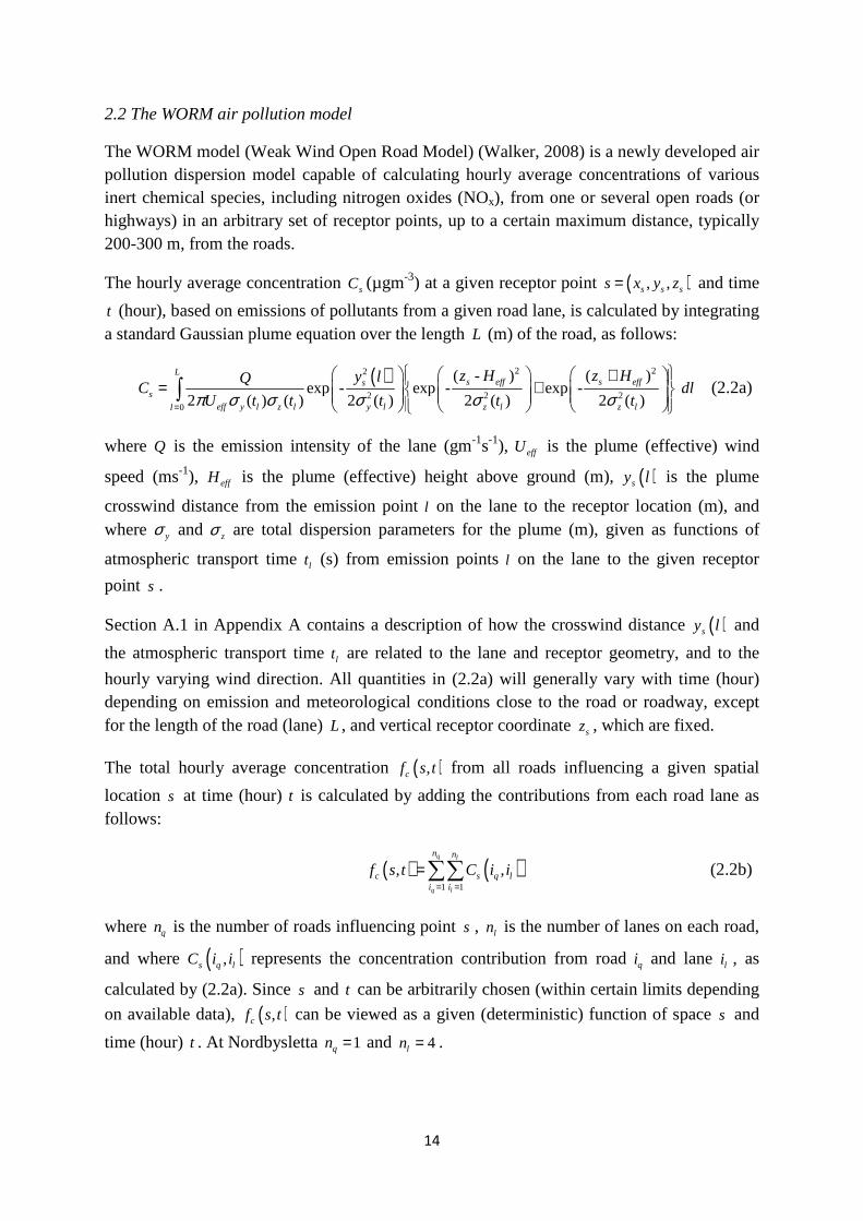
2.2 The WORM air pollution model

The WORM model (Weak Wind Open Road Model) (Walker, 2008) is a newly developed air pollution dispersion model capable of calculating hourly average concentrations of various inert chemical species, including nitrogen oxides (NOx), from one or several open roads (or highways) in an arbitrary set of receptor points, up to a certain maximum distance, typically 200-300 m, from the roads.

The hourly average concentration sC (µgm-3) at a given receptor point ( ), ,s s ss x y z= and time

t (hour), based on emissions of pollutants from a given road lane, is calculated by integrating a standard Gaussian plume equation over the length L (m) of the road, as follows:

( ) 2 22

2 2 20

( - ) ( )exp - exp - exp -

2 ( ) ( ) 2 ( ) 2 ( ) 2 ( )

Ls eff s effs

seff y l z l y l z l z ll

z H z Hy lQC dl

U t t t t tπ σ σ σ σ σ=

+ = +

∫ (2.2a)

where Q is the emission intensity of the lane (gm-1s-1), effU is the plume (effective) wind

speed (ms-1), effH is the plume (effective) height above ground (m), ( )sy l is the plume

crosswind distance from the emission point l on the lane to the receptor location (m), and where yσ and zσ are total dispersion parameters for the plume (m), given as functions of

atmospheric transport time lt (s) from emission points l on the lane to the given receptor

point s .

Section A.1 in Appendix A contains a description of how the crosswind distance ( )sy l and

the atmospheric transport time lt are related to the lane and receptor geometry, and to the

hourly varying wind direction. All quantities in (2.2a) will generally vary with time (hour) depending on emission and meteorological conditions close to the road or roadway, except for the length of the road (lane) L , and vertical receptor coordinate sz , which are fixed.

The total hourly average concentration ( ),cf s t from all roads influencing a given spatial

location s at time (hour) t is calculated by adding the contributions from each road lane as follows:

( ) ( )1 1

, ,q l

q l

n n

c s q li i

f s t C i i= =

=∑∑ (2.2b)

where qn is the number of roads influencing point s , ln is the number of lanes on each road,

and where ( ),s q lC i i represents the concentration contribution from road qi and lane li , as

calculated by (2.2a). Since s and t can be arbitrarily chosen (within certain limits depending

on available data), ( ),cf s t can be viewed as a given (deterministic) function of space s and

time (hour) t . At Nordbysletta 1qn = and 4ln = .

15

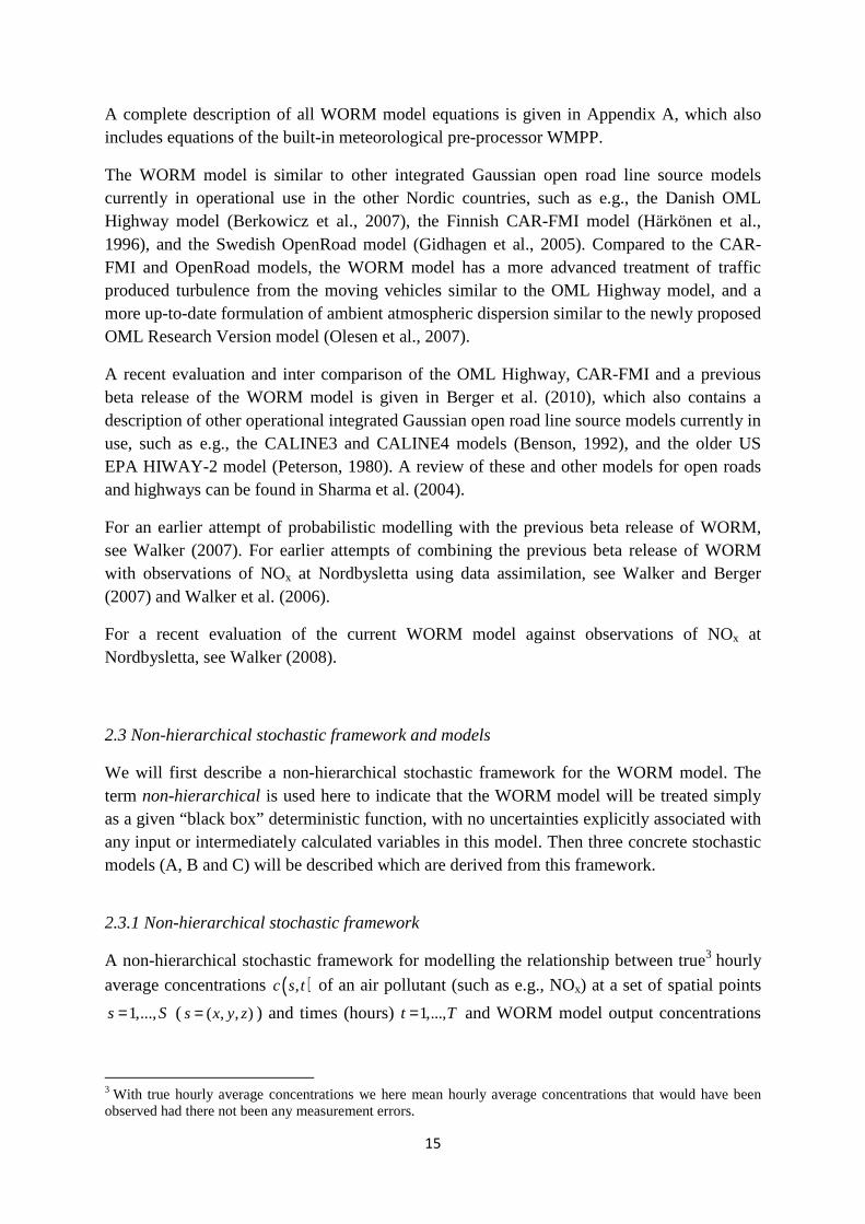
A complete description of all WORM model equations is given in Appendix A, which also includes equations of the built-in meteorological pre-processor WMPP.

The WORM model is similar to other integrated Gaussian open road line source models currently in operational use in the other Nordic countries, such as e.g., the Danish OML Highway model (Berkowicz et al., 2007), the Finnish CAR-FMI model (Härkönen et al., 1996), and the Swedish OpenRoad model (Gidhagen et al., 2005). Compared to the CAR-FMI and OpenRoad models, the WORM model has a more advanced treatment of traffic produced turbulence from the moving vehicles similar to the OML Highway model, and a more up-to-date formulation of ambient atmospheric dispersion similar to the newly proposed OML Research Version model (Olesen et al., 2007).

A recent evaluation and inter comparison of the OML Highway, CAR-FMI and a previous beta release of the WORM model is given in Berger et al. (2010), which also contains a description of other operational integrated Gaussian open road line source models currently in use, such as e.g., the CALINE3 and CALINE4 models (Benson, 1992), and the older US EPA HIWAY-2 model (Peterson, 1980). A review of these and other models for open roads and highways can be found in Sharma et al. (2004).

For an earlier attempt of probabilistic modelling with the previous beta release of WORM, see Walker (2007). For earlier attempts of combining the previous beta release of WORM with observations of NOx at Nordbysletta using data assimilation, see Walker and Berger (2007) and Walker et al. (2006).

For a recent evaluation of the current WORM model against observations of NOx at Nordbysletta, see Walker (2008).

2.3 Non-hierarchical stochastic framework and models

We will first describe a non-hierarchical stochastic framework for the WORM model. The term non-hierarchical is used here to indicate that the WORM model will be treated simply as a given “black box” deterministic function, with no uncertainties explicitly associated with any input or intermediately calculated variables in this model. Then three concrete stochastic models (A, B and C) will be described which are derived from this framework.

2.3.1 Non-hierarchical stochastic framework

A non-hierarchical stochastic framework for modelling the relationship between true3 hourly

average concentrations ( ),c s t of an air pollutant (such as e.g., NOx) at a set of spatial points

1,...,s S= ( ( , , )s x y z= ) and times (hours) 1,...,t T= and WORM model output concentrations

3 With true hourly average concentrations we here mean hourly average concentrations that would have been observed had there not been any measurement errors.

16

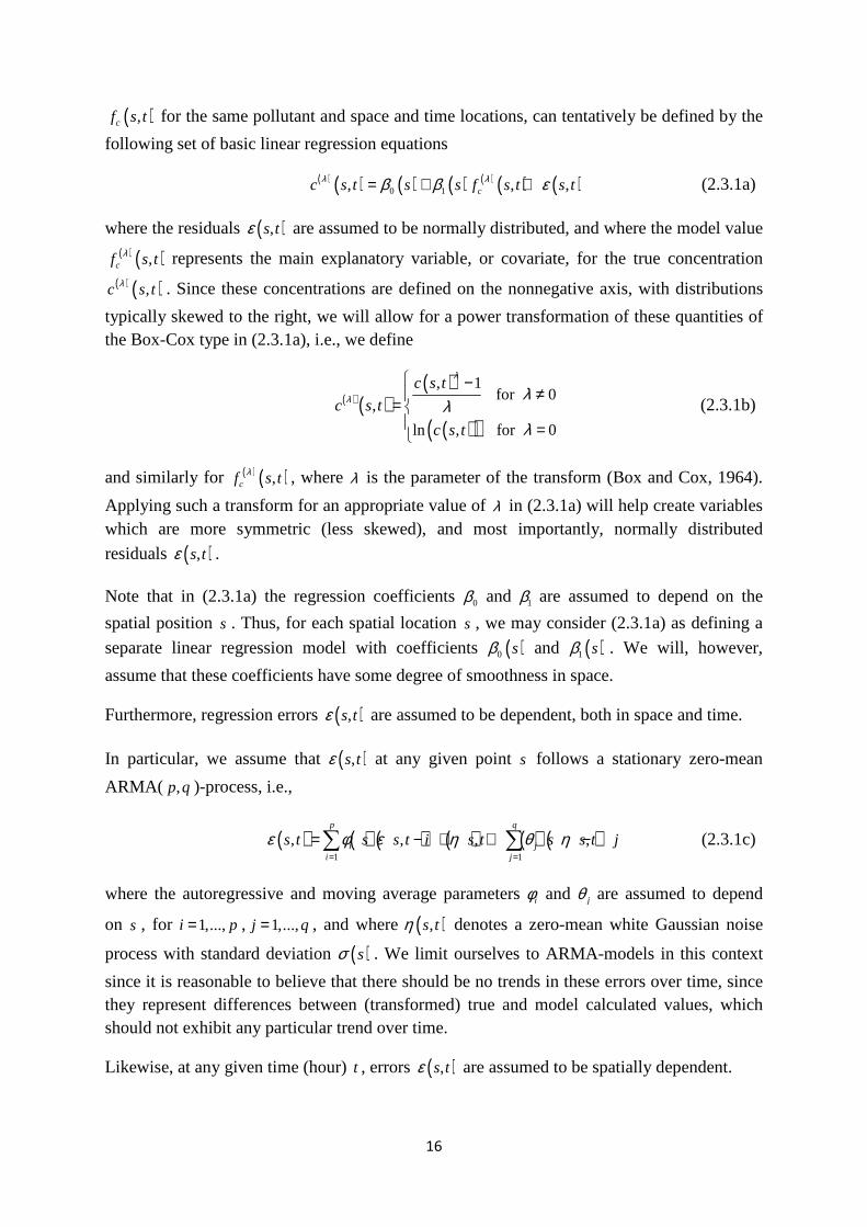
( ),cf s t for the same pollutant and space and time locations, can tentatively be defined by the

following set of basic linear regression equations

( ) ( ) ( ) ( ) ( ) ( ) ( )0 1, , ,cc s t s s f s t s tλ λβ β ε= + + (2.3.1a)

where the residuals ( ),s tε are assumed to be normally distributed, and where the model value ( ) ( ),cf s tλ represents the main explanatory variable, or covariate, for the true concentration

( ) ( ),c s tλ . Since these concentrations are defined on the nonnegative axis, with distributions

typically skewed to the right, we will allow for a power transformation of these quantities of the Box-Cox type in (2.3.1a), i.e., we define

( ) ( )( )

( )( )

, 1 for 0

,

ln , for 0

c s t

c s t

c s t

λ

λ λλ

λ

−≠

= =

(2.3.1b)

and similarly for ( ) ( ),cf s tλ , where λ is the parameter of the transform (Box and Cox, 1964).

Applying such a transform for an appropriate value of λ in (2.3.1a) will help create variables which are more symmetric (less skewed), and most importantly, normally distributed

residuals ( ),s tε .

Note that in (2.3.1a) the regression coefficients 0β and 1β are assumed to depend on the

spatial position s . Thus, for each spatial location s , we may consider (2.3.1a) as defining a

separate linear regression model with coefficients ( )0 sβ and ( )1 sβ . We will, however,

assume that these coefficients have some degree of smoothness in space.

Furthermore, regression errors ( ),s tε are assumed to be dependent, both in space and time.

In particular, we assume that ( ),s tε at any given point s follows a stationary zero-mean

ARMA( ,p q )-process, i.e.,

( ) ( ) ( ) ( ) ( ) ( )1 1

, , , ,p q

i ji j

s t s s t i s t s s t jε φ ε η θ η= =

= − + + −∑ ∑ (2.3.1c)

where the autoregressive and moving average parameters iφ and jθ are assumed to depend

on s , for 1,...,i p= , 1,...,j q= , and where ( ),s tη denotes a zero-mean white Gaussian noise

process with standard deviation ( )sσ . We limit ourselves to ARMA-models in this context

since it is reasonable to believe that there should be no trends in these errors over time, since they represent differences between (transformed) true and model calculated values, which should not exhibit any particular trend over time.

Likewise, at any given time (hour) t , errors ( ),s tε are assumed to be spatially dependent.

17

There are many ways to model such dependencies (Le and Zidek, 2006). One possible approach here is to assume an exponential form for the covariance between the Gaussian

noise terms ( ),s tη at arbitrary locations s and 's , e.g., modelled as follows:

( ) ( )( ) ( ) ( ) ( )( )2cov , , ', ' exp ' ss t s t s s s s

αη η σ σ δ= − − (2.3.1d)

where ( ) ( )( )2Var ,s s tσ η= ;

2's s− denotes the usual 2-norm or Euclidian distance between

the locations s and 's ; sδ is a given distance-scale parameter; and where α is typically set to

e.g., 1 or 2 , depending on the degree of smoothness we seek to obtain.

Modelling spatial or temporal dependencies are important for making multivariate probabilistic predictions, i.e., when we want to calculate the probability distribution of concentrations at several spatial and temporal locations simultaneously. Examples here could be e.g., to calculate the probability that a daily mean value at a given point exceeds a given (limit) value; or to calculate the probability that an average concentration over a given spatial domain at a given hour will exceed a given (limit) value. We could also conceive of applications where we average both in space and time simultaneously. For univariate probabilistic predictions (one-point-at-a-time) in space and time, modelling dependencies will be of minor importance.

In addition to the basic framework equations represented by (2.3a-d), we may also define observation equations

( ) ( ) ( ) ( )( ), ( , ), , , 1,...,m m y my s t H c s t s t m Mλ λ η= =

(2.3.1e)

where M denotes the number of observational points (monitoring stations), and the function

H is an observation operator linking transformed air quality observations ( ) ( ),my s tλ of the

given pollutant with corresponding transformed true concentrations ( ) ( ),mc s tλ at each

measurement point ms , for 1,...,m M= , where ( ),y ms tη represents observational errors. For

air quality observations, it is often the case that such errors can be assumed to be normally distributed and additive, e.g.,

( ) ( ) ( ) ( ) ( ), , , , 1,...,m m y my s t c s t s t m Mλ λ η= + = (2.3.1f)

where ( ) ( )2, 0,iid

y m ys t Nη σ∼ for all observation points ms and times (hours) t .

One of the main assumptions above is that the residual errors ( ),s tε are normally distributed

and follows an ARMA-process. Since the errors represent differences between (transformed) true and regression adjusted modelled concentrations it is not unreasonable to believe that they (theoretically) will form a stationary, zero-mean time series at any given spatial point s . The existence of a Wold decomposition for any such process (Shumway and Stoffer, 2006, Appendix B.4) gives us some confidence that the above residuals might follow an ARMA-

18

process. Furthermore, according to Irwin et al. (2007), differences between observed and model calculated concentrations using Gaussian plume dispersion models are typically lognormally (most cases) or normally distributed, or will have some distribution close to these. Including the Box-Cox transformation parameter in (2.3.1a) thus gives us some confidence that such differences (appropriately transformed) can be modelled in terms of normal distributions.

As stated earlier, the stochastic framework defined in terms of the (state-space) equations (2.3.1a-f) is called non-hierarchical since it does not explicitly address any internal uncertainties in the WORM model itself, but rather treats this model as a given “black box” deterministic function of space and time (and other input data which are given as functions of time). An alternative way of handling modelling uncertainties is to consider uncertainties also in one or several of the internal variables of the WORM model. This leads naturally to a hierarchical approach of handling model uncertainty, which is described in Section 2.4.

In the next three sections, however, we will present three concrete stochastic models (A-C) derived from the above non-hierarchical framework.

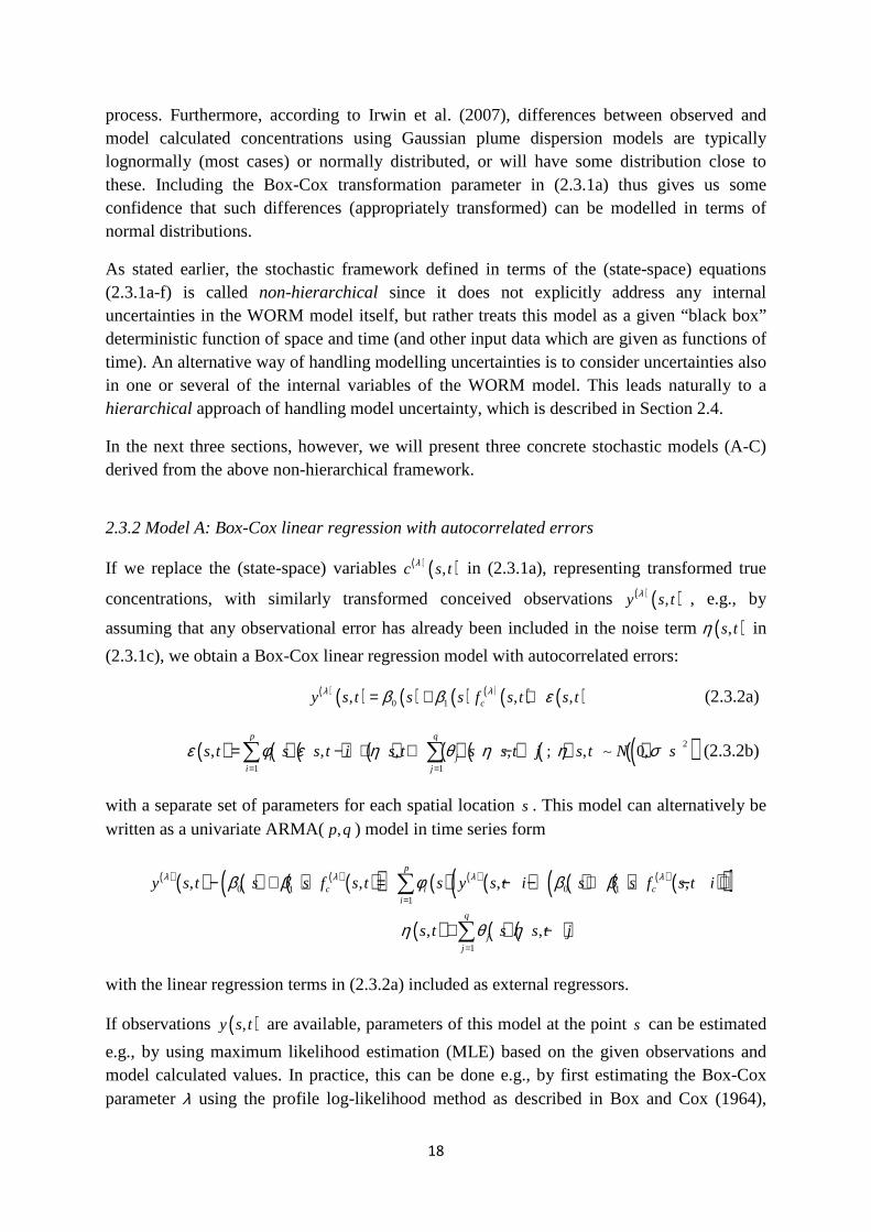
2.3.2 Model A: Box-Cox linear regression with autocorrelated errors

If we replace the (state-space) variables ( ) ( ),c s tλ in (2.3.1a), representing transformed true

concentrations, with similarly transformed conceived observations ( ) ( ),y s tλ , e.g., by

assuming that any observational error has already been included in the noise term ( ),s tη in

(2.3.1c), we obtain a Box-Cox linear regression model with autocorrelated errors:

( ) ( ) ( ) ( ) ( ) ( ) ( )0 1, , ,cy s t s s f s t s tλ λβ β ε= + + (2.3.2a)

( ) ( ) ( ) ( ) ( ) ( ) ( ) ( )( )2

1 1

, , , , ; , 0,p q

i ji j

s t s s t i s t s s t j s t N sε φ ε η θ η η σ= =

= − + + −∑ ∑ ∼ (2.3.2b)

with a separate set of parameters for each spatial location s . This model can alternatively be written as a univariate ARMA(,p q ) model in time series form

( ) ( ) ( ) ( ) ( ) ( )( ) ( ) ( ) ( ) ( ) ( ) ( ) ( )( )( )( ) ( ) ( )

0 1 0 11

1

, , , ,

, ,

p

c i ci

q

jj

y s t s s f s t s y s t i s s f s t i

s t s s t j

λ λ λ λβ β φ β β

η θ η

=

=

− + = − − + − +

+ −

∑

∑

with the linear regression terms in (2.3.2a) included as external regressors.

If observations ( ),y s t are available, parameters of this model at the point s can be estimated

e.g., by using maximum likelihood estimation (MLE) based on the given observations and model calculated values. In practice, this can be done e.g., by first estimating the Box-Cox parameter λ using the profile log-likelihood method as described in Box and Cox (1964),

19

using independent data from the original time series of observed and model calculated values, e.g., every n th value of the series, for large enough n , to make the data independent, and then

estimating the other parameters in the model using the transformed observations ( )( ) ,y s tλ and

model calculated values ( ) ( ),cf s tλ . The latter can e.g., be accomplished using the R-routine

ARIMA since this is capable of including external regressors in the ARMA-model and is also able to handle missing data since it is based internally on a Kalman filter.

In order to be able to use this model also at spatial locations where there are no observations, we need somehow to interpolate or extrapolate estimated parameters from the observation points ms , 1,...,m M= , to any new location s . We prefer here to interpolate or extrapolate

parameters to the new point s , rather than interpolating predictions, since we prefer to use

the actual model calculated value ( ),cf s t at the point s , rather than interpolated values of

( ),c mf s t from the observation points. Interpolation of parameters can be accomplished by

using spatial interpolation techniques, such as e.g., Kriging (Le and Zidek, 2006), or simply by selecting a nearby representative point ms and use the estimated model parameters from

this point also at location s . Special care must be taken when e.g., interpolating the parameters of the ARMA-models to ensure that the resulting new model remains causal and invertible.

In practice, there will usually not be many observations available close to roads in a city or urban area, so in most cases M will be relatively small, e.g., typically in the range 1-10. The procedure of interpolating or extrapolating parameters will, therefore, only work if the true parameters do not vary too much over the area of interest.

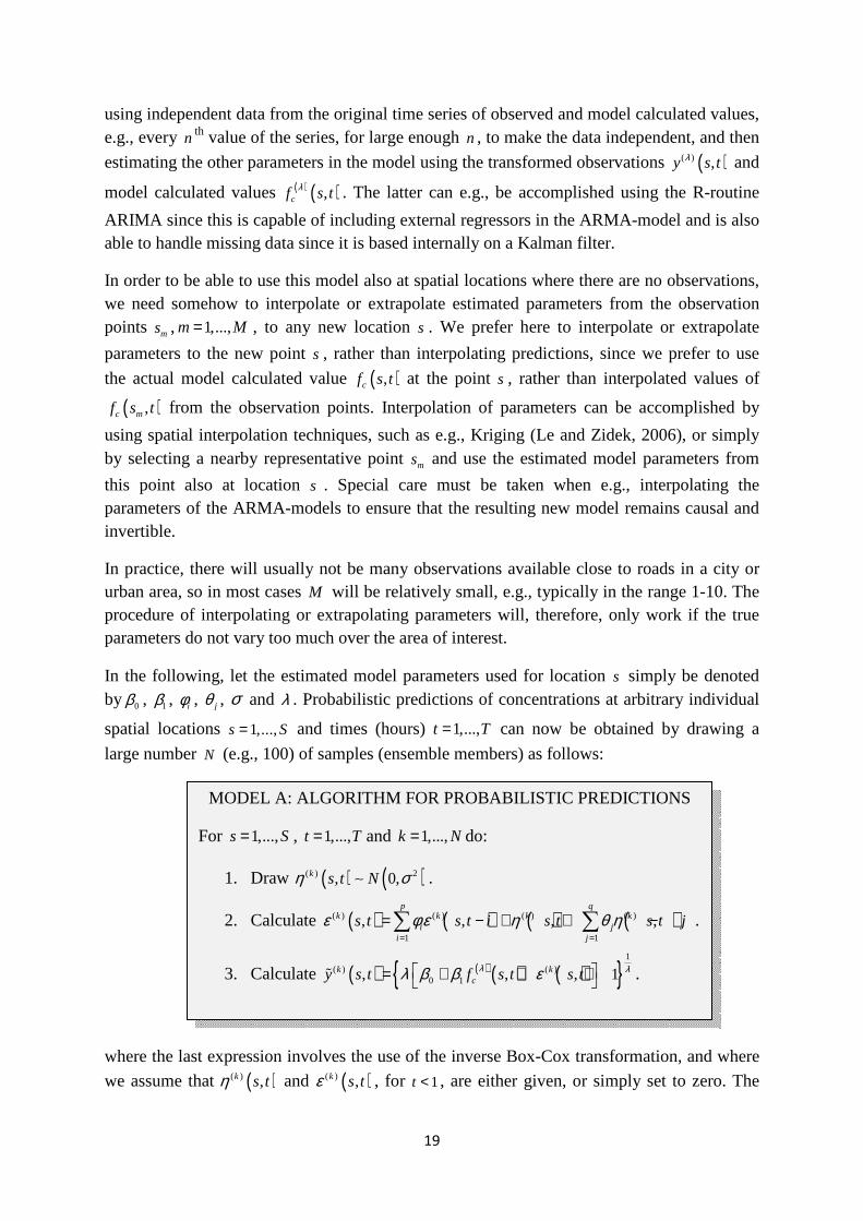
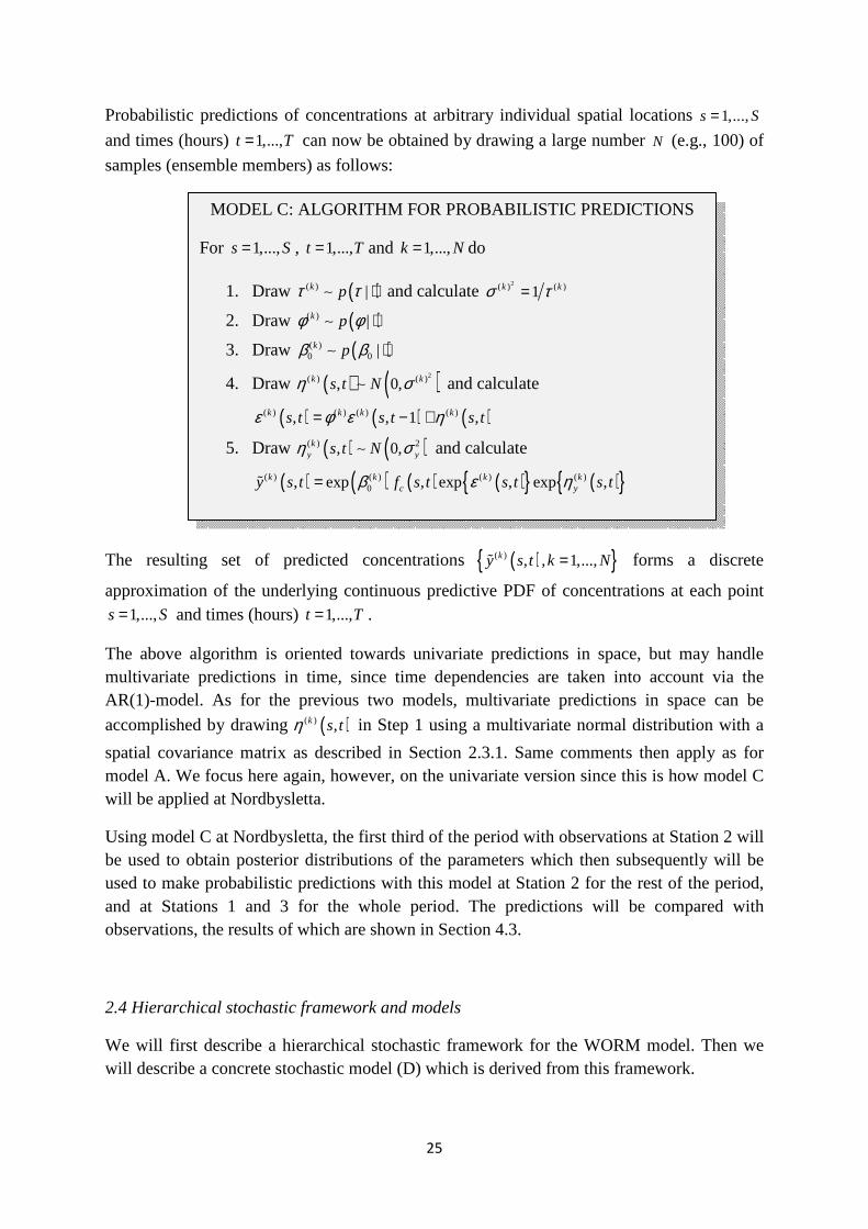
In the following, let the estimated model parameters used for location s simply be denoted by 0β , 1β , iφ , jθ , σ and λ . Probabilistic predictions of concentrations at arbitrary individual

spatial locations 1,...,s S= and times (hours) 1,...,t T= can now be obtained by drawing a

large number N (e.g., 100) of samples (ensemble members) as follows:

where the last expression involves the use of the inverse Box-Cox transformation, and where

we assume that ( )( ) ,k s tη and ( )( ) ,k s tε , for 1t < , are either given, or simply set to zero. The

MODEL A: ALGORITHM FOR PROBABILISTIC PREDICTIONS

For 1,...,s S= , 1,...,t T= and 1,...,k N= do:

1. Draw ( ) ( )( ) 2, 0,k s t Nη σ∼ .

2. Calculate ( ) ( ) ( ) ( )( ) ( ) ( ) ( )

1 1

, , , ,p q

k k k ki j

i j

s t s t i s t s t jε φ ε η θ η= =

= − + + −∑ ∑ .

3. Calculate ( ) ( ) ( ) ( ) 1

( ) ( )0 1, , , 1k k

cy s t f s t s tλ λλ β β ε = + + + ɶ .

20

resulting set of predicted concentration values ( ) ( ) , , 1,...,ky s t k N=ɶ then forms a discrete

approximation of the underlying continuous predictive PDF of concentrations at each point 1,...,s S= and times (hours) 1,...,t T= .

The above algorithm is oriented towards univariate (one-point-at-a-time) predictions in space, but is able to handle multivariate predictions in time, since time dependencies are taken into account via the ARMA model. Multivariate predictions in space can be accomplished by

drawing ( )( ) ,k s tη in Step 1 of the above procedure using a multivariate normal distribution

with a spatial covariance matrix as described in Section 2.3.1, but in practice it might be difficult to obtain estimates of the distance scale parameter sδ in (2.3.1d), at least we need

then several observations, and even then it might be difficult since we only have one set of estimated parameters at each spatial point. It may be necessary then, to use just some predetermined value for this parameter in order to obtain smoothness in space. We focus here, however, on the univariate version since this is the way model A will be applied at Nordbysletta.

Using model A at Nordbysletta, the first third of the period (840 hours) with observations at Station 2 will be used to obtain parameter estimates, which then will be used to make probabilistic predictions with this model at the same station for the rest of the period, and at Stations 1 and 3 for the whole period. The predictions will be compared with corresponding (independent) observations at the stations, the results of which are shown in Section 4.1.

2.3.3 Model B: Bayesian non-hierarchical prior predictive model

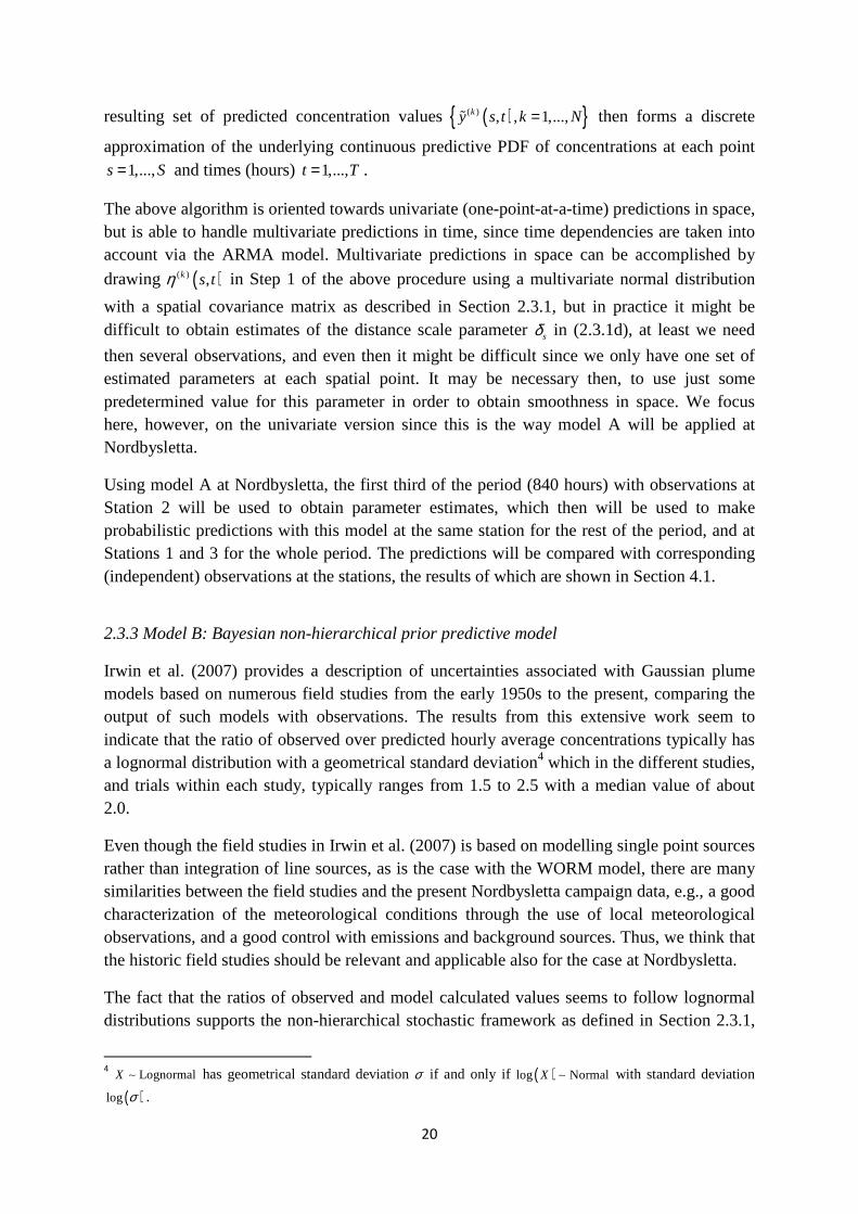
Irwin et al. (2007) provides a description of uncertainties associated with Gaussian plume models based on numerous field studies from the early 1950s to the present, comparing the output of such models with observations. The results from this extensive work seem to indicate that the ratio of observed over predicted hourly average concentrations typically has a lognormal distribution with a geometrical standard deviation4 which in the different studies, and trials within each study, typically ranges from 1.5 to 2.5 with a median value of about 2.0.

Even though the field studies in Irwin et al. (2007) is based on modelling single point sources rather than integration of line sources, as is the case with the WORM model, there are many similarities between the field studies and the present Nordbysletta campaign data, e.g., a good characterization of the meteorological conditions through the use of local meteorological observations, and a good control with emissions and background sources. Thus, we think that the historic field studies should be relevant and applicable also for the case at Nordbysletta.

The fact that the ratios of observed and model calculated values seems to follow lognormal distributions supports the non-hierarchical stochastic framework as defined in Section 2.3.1,

4 LognormalX ∼ has geometrical standard deviation σ if and only if ( )log NormalX ∼ with standard deviation

( )log σ .

21

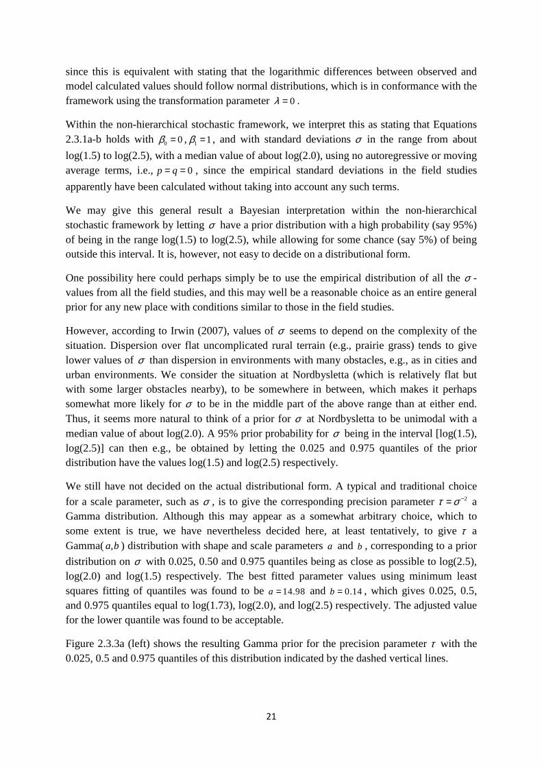
since this is equivalent with stating that the logarithmic differences between observed and model calculated values should follow normal distributions, which is in conformance with the framework using the transformation parameter 0λ = .

Within the non-hierarchical stochastic framework, we interpret this as stating that Equations 2.3.1a-b holds with 0 0β = , 1 1β = , and with standard deviations σ in the range from about

log(1.5) to log(2.5), with a median value of about log(2.0), using no autoregressive or moving average terms, i.e., 0p q= = , since the empirical standard deviations in the field studies

apparently have been calculated without taking into account any such terms.

We may give this general result a Bayesian interpretation within the non-hierarchical stochastic framework by letting σ have a prior distribution with a high probability (say 95%) of being in the range log(1.5) to log(2.5), while allowing for some chance (say 5%) of being outside this interval. It is, however, not easy to decide on a distributional form.

One possibility here could perhaps simply be to use the empirical distribution of all the σ -values from all the field studies, and this may well be a reasonable choice as an entire general prior for any new place with conditions similar to those in the field studies.

However, according to Irwin (2007), values of σ seems to depend on the complexity of the situation. Dispersion over flat uncomplicated rural terrain (e.g., prairie grass) tends to give lower values of σ than dispersion in environments with many obstacles, e.g., as in cities and urban environments. We consider the situation at Nordbysletta (which is relatively flat but with some larger obstacles nearby), to be somewhere in between, which makes it perhaps somewhat more likely for σ to be in the middle part of the above range than at either end. Thus, it seems more natural to think of a prior for σ at Nordbysletta to be unimodal with a median value of about log(2.0). A 95% prior probability for σ being in the interval [log(1.5), log(2.5)] can then e.g., be obtained by letting the 0.025 and 0.975 quantiles of the prior distribution have the values log(1.5) and log(2.5) respectively.

We still have not decided on the actual distributional form. A typical and traditional choice

for a scale parameter, such as σ , is to give the corresponding precision parameter 2τ σ −= a Gamma distribution. Although this may appear as a somewhat arbitrary choice, which to some extent is true, we have nevertheless decided here, at least tentatively, to give τ a Gamma( ,a b) distribution with shape and scale parameters a and b , corresponding to a prior

distribution on σ with 0.025, 0.50 and 0.975 quantiles being as close as possible to log(2.5), log(2.0) and log(1.5) respectively. The best fitted parameter values using minimum least squares fitting of quantiles was found to be 14.98a = and 0.14b = , which gives 0.025, 0.5, and 0.975 quantiles equal to log(1.73), log(2.0), and log(2.5) respectively. The adjusted value for the lower quantile was found to be acceptable.

Figure 2.3.3a (left) shows the resulting Gamma prior for the precision parameter τ with the 0.025, 0.5 and 0.975 quantiles of this distribution indicated by the dashed vertical lines.

22

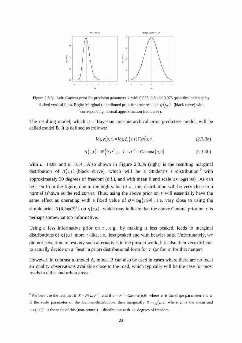
Figure 2.3.3a. Left: Gamma prior for precision parameter τ with 0.025, 0.5 and 0.975 quantiles indicated by

dashed vertical lines. Right: Marginal t-distributed prior for error residual ( ),s tη (black curve) with

corresponding normal approximation (red curve).

The resulting model, which is a Bayesian non-hierarchical prior predictive model, will be called model B. It is defined as follows:

( ) ( ) ( )log , log , ,cy s t f s t s tη= + (2.3.3a)

( ) ( ) ( )2 2, 0, ; Gamma ,s t N a bη σ τ σ −=∼ ∼ (2.3.3b)

with 14.98a = and 0.14b = . Also shown in Figure 2.3.3a (right) is the resulting marginal

distribution of ( ),s tη (black curve), which will be a Student’s t -distribution5 with

approximately 30 degrees of freedom (d.f.), and with mean 0 and scale log(1.99)s ≈ . As can

be seen from the figure, due to the high value of a , this distribution will be very close to a normal (shown as the red curve). Thus, using the above prior on τ will essentially have the

same effect as operating with a fixed value of ( )log 1.99σ ≈ , i.e. very close to using the

simple prior ( )20,log(2)N on ( ),s tη , which may indicate that the above Gamma prior on τ is

perhaps somewhat too informative.

Using a less informative prior on τ , e.g., by making it less peaked, leads to marginal

distributions of ( ),s tη more t -like, i.e., less peaked and with heavier tails. Unfortunately, we

did not have time to test any such alternatives in the present work. It is also then very difficult to actually decide on a “best” a priori distributional form for τ (or for σ for that matter).

However, in contrast to model A, model B can also be used in cases where there are no local air quality observations available close to the road, which typically will be the case for most roads in cities and urban areas.

5 We here use the fact that if ( )2,X N µ σ∼ , and if ( )2 Gamma ,a bτ σ −= ∼ where a is the shape parameter and b

is the scale parameter of the Gamma-distribution, then marginally ( )2 ,aX t sµ∼ where µ is the mean and

( )12s ab

−= is the scale of this (non-central) t -distribution with 2a degrees of freedom.

0 1 2 3 4 5 6 7

0.0

0.2

0.4

0.6

Prior for tau

tau

Dis

tribu

tion

-2 -1 0 1 2

0.0

0.1

0.2

0.3

0.4

Marginal prior for eta

eta

Dis

tribu

tion

23

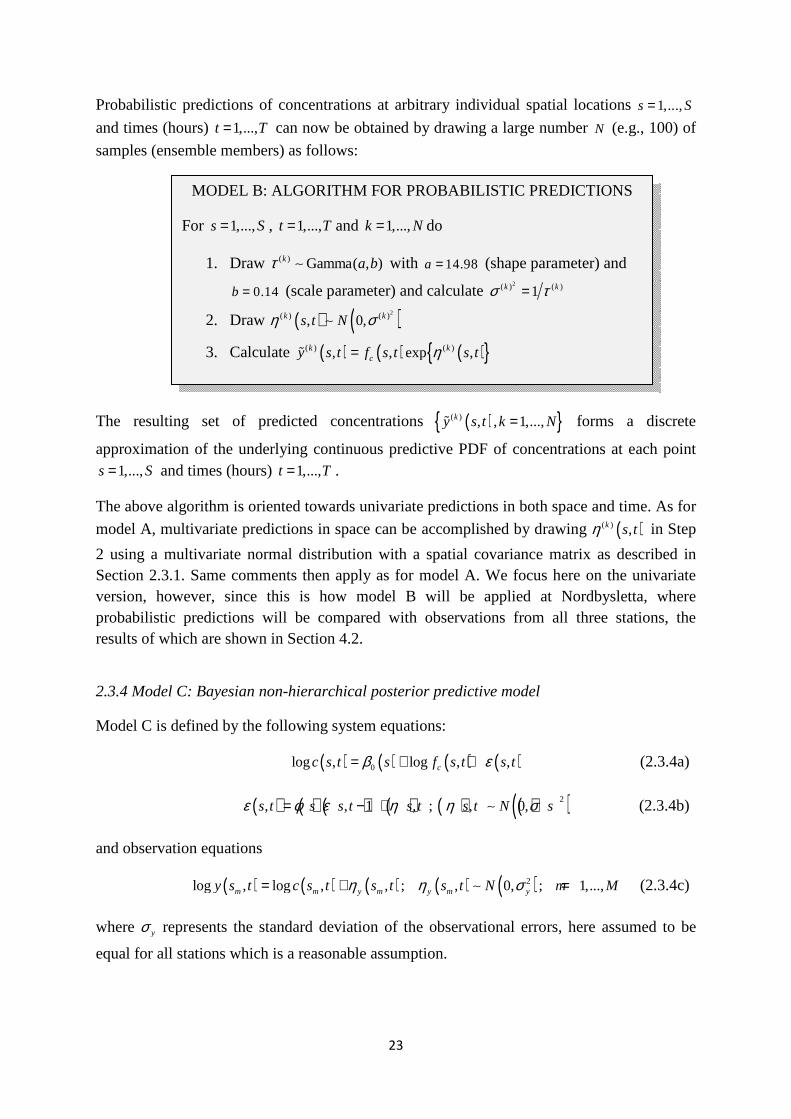
Probabilistic predictions of concentrations at arbitrary individual spatial locations 1,...,s S=

and times (hours) 1,...,t T= can now be obtained by drawing a large number N (e.g., 100) of

samples (ensemble members) as follows:

The resulting set of predicted concentrations ( ) ( ) , , 1,...,ky s t k N=ɶ forms a discrete


The above algorithm is oriented towards univariate predictions in both space and time. As for

model A, multivariate predictions in space can be accomplished by drawing ( )( ) ,k s tη in Step

2 using a multivariate normal distribution with a spatial covariance matrix as described in Section 2.3.1. Same comments then apply as for model A. We focus here on the univariate version, however, since this is how model B will be applied at Nordbysletta, where probabilistic predictions will be compared with observations from all three stations, the results of which are shown in Section 4.2.

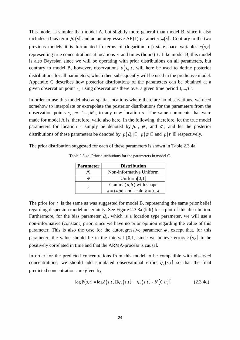
2.3.4 Model C: Bayesian non-hierarchical posterior predictive model

Model C is defined by the following system equations:

( ) ( ) ( ) ( )0log , log , ,cc s t s f s t s tβ ε= + + (2.3.4a)

( ) ( ) ( ) ( ) ( ) ( )( )2, , 1 , ; , 0,s t s s t s t s t N sε φ ε η η σ= − + ∼ (2.3.4b)

and observation equations

( ) ( ) ( ) ( ) ( )2log , log , , ; , 0, ; 1,...,m m y m y m yy s t c s t s t s t N m Mη η σ= + =∼ (2.3.4c)

where yσ represents the standard deviation of the observational errors, here assumed to be

equal for all stations which is a reasonable assumption.

MODEL B: ALGORITHM FOR PROBABILISTIC PREDICTIONS

For 1,...,s S= , 1,...,t T= and 1,...,k N= do

1. Draw ( ) Gamma( , )k a bτ ∼ with 14.98a = (shape parameter) and

0.14b = (scale parameter) and calculate 2( ) ( )1k kσ τ=

2. Draw ( ) ( )2( ) ( ), 0,k ks t Nη σ∼

3. Calculate ( ) ( ) ( ) ( ) ( ), , exp ,k kcy s t f s t s tη=ɶ

24

This model is simpler than model A, but slightly more general than model B, since it also

includes a bias term ( )0 sβ and an autoregressive AR(1) parameter ( )sφ . Contrary to the two

previous models it is formulated in terms of (logarithm of) state-space variables ( ),c s t

representing true concentrations at locations s and times (hours) t . Like model B, this model is also Bayesian since we will be operating with prior distributions on all parameters, but

contrary to model B, however, observations ( ),my s t will here be used to define posterior

distributions for all parameters, which then subsequently will be used in the predictive model. Appendix C describes how posterior distributions of the parameters can be obtained at a given observation point ms using observations there over a given time period 1,..., 'T .

In order to use this model also at spatial locations where there are no observations, we need somehow to interpolate or extrapolate the posterior distributions for the parameters from the observation points ms , 1,...,m M= , to any new location s . The same comments that were

made for model A is, therefore, valid also here. In the following, therefore, let the true model parameters for location s simply be denoted by0β , φ , and σ , and let the posterior

distributions of these parameters be denoted by ( )0 |p β ⋅ , ( )|p φ ⋅ and ( )|p τ ⋅ respectively.

The prior distribution suggested for each of these parameters is shown in Table 2.3.4a.

Table 2.3.4a. Prior distributions for the parameters in model C.

Parameter Distribution 0β Non-informative Uniform

φ Uniform[0,1]

τ Gamma( ,a b) with shape

14.98a = and scale 0.14b =

The prior for τ is the same as was suggested for model B, representing the same prior belief regarding dispersion model uncertainty. See Figure 2.3.3a (left) for a plot of this distribution. Furthermore, for the bias parameter 0β , which is a location type parameter, we will use a

non-informative (constant) prior, since we have no prior opinion regarding the value of this parameter. This is also the case for the autoregressive parameter φ , except that, for this

parameter, the value should lie in the interval [0,1] since we believe errors ( ),s tε to be

positively correlated in time and that the ARMA-process is causal.

In order for the predicted concentrations from this model to be compatible with observed concentrations, we should add simulated observational errors ( ),y s tη so that the final

predicted concentrations are given by

( ) ( ) ( ) ( ) ( )2log , log , , ; , 0,y y yy s t c s t s t s t Nη η σ= +ɶ ɶ ∼ . (2.3.4d)

25

Probabilistic predictions of concentrations at arbitrary individual spatial locations 1,...,s S=

and times (hours) 1,...,t T= can now be obtained by drawing a large number N (e.g., 100) of

samples (ensemble members) as follows:



The above algorithm is oriented towards univariate predictions in space, but may handle multivariate predictions in time, since time dependencies are taken into account via the AR(1)-model. As for the previous two models, multivariate predictions in space can be

accomplished by drawing ( )( ) ,k s tη in Step 1 using a multivariate normal distribution with a

spatial covariance matrix as described in Section 2.3.1. Same comments then apply as for model A. We focus here again, however, on the univariate version since this is how model C will be applied at Nordbysletta.

Using model C at Nordbysletta, the first third of the period with observations at Station 2 will be used to obtain posterior distributions of the parameters which then subsequently will be used to make probabilistic predictions with this model at Station 2 for the rest of the period, and at Stations 1 and 3 for the whole period. The predictions will be compared with observations, the results of which are shown in Section 4.3.

2.4 Hierarchical stochastic framework and models

We will first describe a hierarchical stochastic framework for the WORM model. Then we will describe a concrete stochastic model (D) which is derived from this framework.

MODEL C: ALGORITHM FOR PROBABILISTIC PREDICTIONS

For 1,...,s S= , 1,...,t T= and 1,...,k N= do

1. Draw ( )( ) |k pτ τ ⋅∼ and calculate 2( ) ( )1k kσ τ=

2. Draw ( )( ) |k pφ φ ⋅∼

3. Draw ( )( )0 0 |k pβ β ⋅∼

4. Draw ( ) ( )2( ) ( ), 0,k ks t Nη σ∼ and calculate

( ) ( ) ( )( ) ( ) ( ) ( ), , 1 ,k k k ks t s t s tε φ ε η= − +

5. Draw ( ) ( )( ) 2, 0,ky ys t Nη σ∼ and calculate

( ) ( ) ( ) ( ) ( ) ( ) ( ) ( ) ( )0, exp , exp , exp ,k k k k

c yy s t f s t s t s tβ ε η=ɶ

The term hierarchical is used here to indicatewith input and intermediate variablesaddition to any final model output uncertainty.

By modelling more precisely through the numerical model,of model output concentrations can be achieved by using predictive distributions from nondoing so, in a sense try to mimicsufficiently close to the real processthrough the model.

2.4.1 Hierarchical stochastic framework

Uncertainties and errors in the inevitably lead to uncertainties and errors model, as well as in the final calculated in the model in a expressions (functions or equationshierarchical framework for describing the

To fix ideas, let 1 2, ,..., rv v v denote

of generality, we may assume hereordered according to the flowcalculates variable kv at time (hour)

where kf denotes the deterministic model func

and where ( )pa kv denotes the vector of other

the parents of kv using graph-

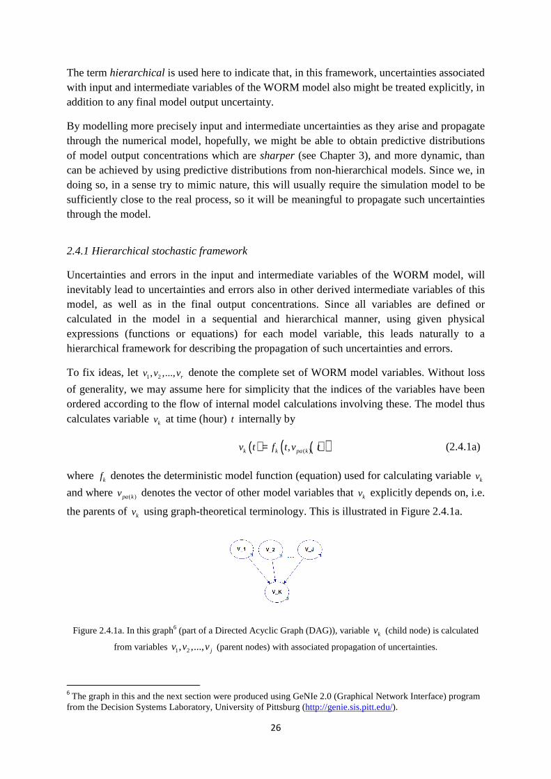
Figure 2.4.1a. In this graph6 (part of a Directed Acyclic G

from variables 1 2, ,...,v v v

6 The graph in this and the next section were produced using GeNIe 2.0 (Graphical Network Interface) program

from the Decision Systems Laboratory, University of Pittsburg (

26

is used here to indicate that, in this framework, uncertainties associatevariables of the WORM model also might be treated

final model output uncertainty.

y modelling more precisely input and intermediate uncertainties as they arise and propagate , hopefully, we might be able to obtain predictive

concentrations which are sharper (see Chapter 3), and more dynamic, than can be achieved by using predictive distributions from non-hierarchical models

try to mimic nature, this will usually require the simulation real process, so it will be meaningful to propagate such

2.4.1 Hierarchical stochastic framework

the input and intermediate variables of the WORM o uncertainties and errors also in other derived intermediate

final output concentrations. Since all variables in a sequential and hierarchical manner, usinequations) for each model variable, this leads

framework for describing the propagation of such uncertainties

denote the complete set of WORM model variables.

assume here for simplicity that the indices of the variables according to the flow of internal model calculations involving these

at time (hour) t internally by

( ) ( )( )( ),k k pa kv t f t v t=

denotes the deterministic model function (equation) used for calculating

denotes the vector of other model variables that kv explicitly

-theoretical terminology. This is illustrated in Figure 2.4.1a.

(part of a Directed Acyclic Graph (DAG)), variable kv (child node)

, ,..., jv v v (parent nodes) with associated propagation of uncertainties.

The graph in this and the next section were produced using GeNIe 2.0 (Graphical Network Interface) program from the Decision Systems Laboratory, University of Pittsburg (http://genie.sis.pitt.edu/).

uncertainties associated treated explicitly, in

uncertainties as they arise and propagate predictive distributions

(see Chapter 3), and more dynamic, than hierarchical models. Since we, in

simulation model to be meaningful to propagate such uncertainties

WORM model, will diate variables of this

variables are defined or , using given physical

leads naturally to a propagation of such uncertainties and errors.

the complete set of WORM model variables. Without loss

of the variables have been these. The model thus

(2.4.1a)

calculating variable kv

explicitly depends on, i.e.

illustrated in Figure 2.4.1a.

(child node) is calculated

with associated propagation of uncertainties.

The graph in this and the next section were produced using GeNIe 2.0 (Graphical Network Interface) program

27

The figure shows a graph depicting a model variable kv , the child node, being calculated

from model variables 1v , 2v , …, jv , the parent nodes (for simplicity assumed here to be the

nodes 1 toj ).

If one or more of the input variables are uncertain, this uncertainty will also propagate to the calculated output variable through (2.4.1a). Also, since no variables are used, either directly or indirectly, to calculate itself, the resulting graph of all nodes (variables) and arcs (dependencies) will necessarily be a Directed Acyclic Graph, or DAG.

Ultimately, in this framework, the last model variable rv to be calculated is the model output

concentration. This is the only WORM model variable that (in addition to time) also will depend on the spatial location s , and is calculated by

( ) ( )( )( ), , ,r r pa rv s t f s t v t= (2.4.1b)

where rf is the same function cf as used in (2.3.1a) and (2.2b), but where we now explicitly

have included the vector ( )pa rv of parent variables that rv depend on as arguments to this

function.

We will now describe the corresponding hierarchical stochastic framework.

For each uncertain input or intermediate model variable kv , 1,..., 1k r= − , which we explicitly

want to model, we will introduce a corresponding (state-space) variable kx representing the

conceived underlying true7 value of this variable. Each variable ( )kx t is then assumed to

evolve in time according to the following set of linear regression equations

( ) ( ) ( ) ( )( ) ( )0 1 ( ),k k

k k k k pa k kx t f t x t tλ λβ β ε= + + (2.4.1c)

where kf represents the deterministic model function for model variable kv as used in

(2.4.1a), and where kλ represents the possible use of a local Box-Cox power transform

parameter. In (2.4.1c), 0kβ and 1kβ represents local regression coefficients for variable k ,

while the error terms ( )k tε are assumed to be dependent in time. In particular, we will

assume ( )k tε to be normal and follow a stationary zero-mean ARMA( ,k kp q )-process, i.e.,

( ) ( ) ( ) ( ) ( ) ( )2

1 1

; 0,k kp q

k ik k jk k k ki j

t t i t t j t Nε φ ε η θ η η σ= =

= − + + −∑ ∑ ∼ (2.4.1d)

for 1,..., 1k r= − . We limit ourselves to ARMA-models in this context since it is reasonable to

believe that there are no trends in such errors over time, since they represent differences between (power transformed) true and model calculated values of the given variable, which should not show any particular trend over time.

7 For some such variables it may be difficult to give a precise definition of what we mean by a true value. We

will attempt to give such definitions for the variables of model D in the next section.

28

For the last (state-space) variable ( ),rx s t , representing true concentration at point s and time

(hour) t , we may use the same stochastic model as described in Section 2.3, i.e.

( ) ( ) ( ) ( ) ( ) ( )( ) ( )0 1 ( ), , , ,r r

r r r r pa r rx s t s s f s t x t s tλ λβ β ε= + + (2.4.1e)

( ) ( ) ( ) ( ) ( ) ( ) ( ) ( )( )2

1 1

, , , , ; , 0,r rp q

r ir r jr r r ri j

s t s s t i s t s s t j s t N sε φ ε η θ η η σ= =

= − + + −∑ ∑ ∼ (2.4.1f)

where model output concentration rf represents the main explanatory variable or covariate

for the true concentration rx . In (2.4.1e) regression coefficients 0rβ and 1rβ are again assumed to

be dependent on the location s , and multivariate predictions can be performed as described in

Section 2.3, e.g., by drawing ( ),r s tη as a multivariate normal with a given spatial covariance

matrix.

It is possible to include observation equations for (transformed) model variables ( )( )kkx tλ by

using equations similar to (2.3.1e-f). Furthermore, we may want to include, for physical reasons, truncation of some of the variables, either from above, from below or both.

In some cases, dependencies may exist between variables that we may wish to include in a more direct way than through the flow of model calculations, e.g., between input variables.

Also, in the above hierarchical stochastic framework we have tacitly assumed that residual

errors kε are independent of explanatory variables( )kkf

λ . This may well be an unrealistic

assumption in many cases (Goldstein and Rougier, 2008). One may, therefore, envision extensions of the above framework where such dependencies are modelled, e.g., using methods such as dependence vines and copulas (Kurowicka and Cooke, 2006).

Finally, on the negative side, it must also be said that, due to the large number of parameters, models derived from the above framework might well encounter problems of identifiability.

2.4.2 Model D: Bayesian hierarchical prior predictive model

Based on general knowledge about uncertainties in Gaussian plume modelling (Irwin et al., 2007), and an extensive sensitivity analysis performed with the WORM model using data from Nordbysletta (not shown here), the following three model variables were selected to be included in a Bayesian hierarchical prior predictive model, which will be called model D:

• Effective plume height effH

• Wind speed at 10 m above ground 10mu

• Wind direction at 10 m above ground 10mϕ

(The total dispersion parameter zσ could also have been included here, but, unfortunately, we

did not have time to do this in the present work.)

29

Bayesian uncertainty models for the above three variables have been developed partly using local meteorological and dispersion modelling expertise at NILU (Tønnesen, 2010), and partly from Irwin et al. (2007), providing a characterization of typical uncertainties in local meteorological parameters associated with Gaussian plume models based on a large number of field studies.

As stated earlier, a potential benefit, in our view, with hierarchical models, such as model D, as compared with the previous non-hierarchical models, is that, by propagating some of the uncertainties through the model, we might be able to achieve predictive distributions of modelled concentrations which are sharper, and more dynamic, than predictive distributions obtained using non-hierarchical models. This, however, requires the model to be sufficiently close to the real process in the atmosphere and that uncertainties that we specify, more or less subjectively if we use the Bayesian approach, be close to the actual uncertainties of the variables involved, the latter of which might not be an easy task. We will describe this somewhat more concretely at the end of this section.

A tentative uncertainty model for the true, effective plume height effH 8

at time (hour) t is

defined as (Tønnesen, 2010)

( ) ( ) ( ) ( ) ( ) ( )2; 0, ; 1eff eff eff effeff H H H H effH t f t t t N H tη η σ= + ≥∼

m (2.4.2a)

where ( ) 3effHf t =

m (constant for all hours).

The precision parameter 2

eff effH Hτ σ −= is here given a Gamma distribution with parameters as

shown in Table 2.4.2a, corresponding to a prior distribution on effHσ with 0.025, 0.5 and

0.975 quantiles equal to 0.6 m, 0.75 m and 1.0 m respectively.

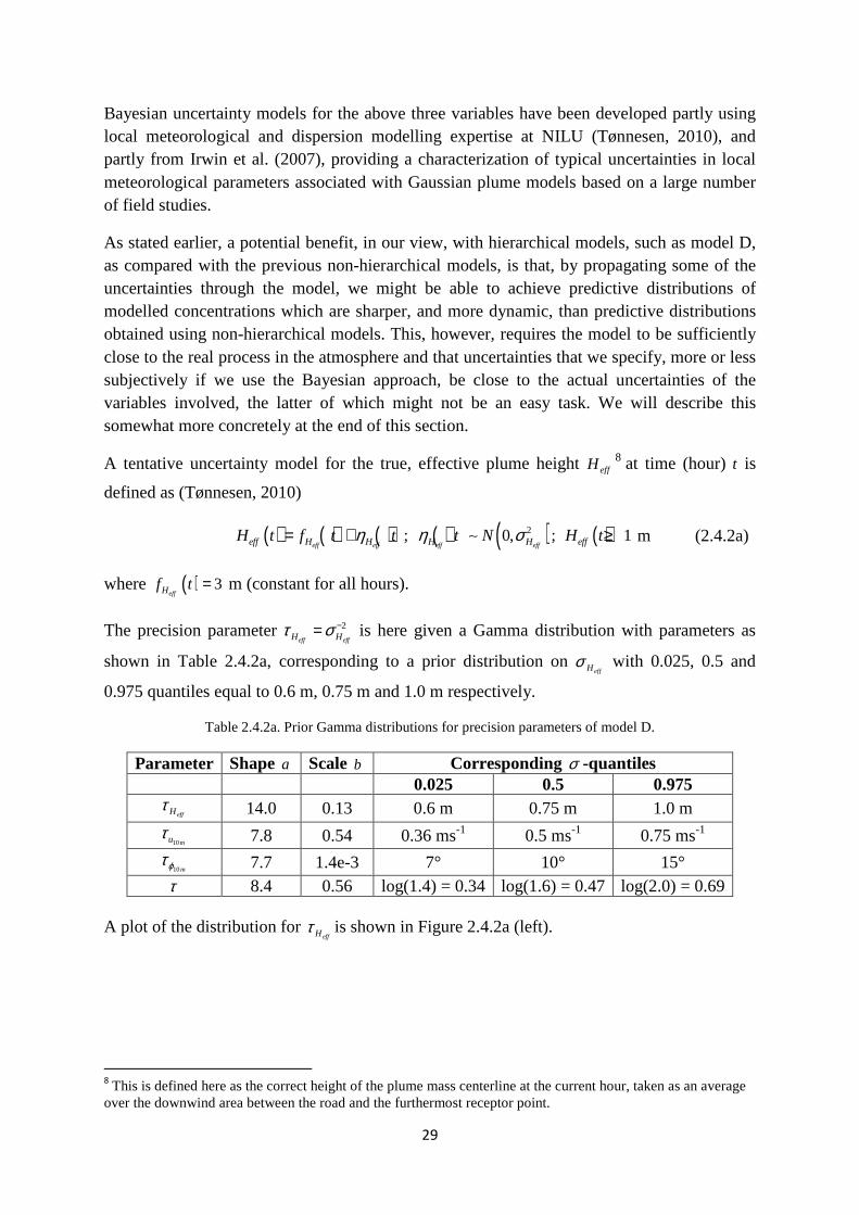
Table 2.4.2a. Prior Gamma distributions for precision parameters of model D.

Parameter Shape a Scale b Corresponding σ -quantiles 0.025 0.5 0.975

effHτ 14.0 0.13 0.6 m 0.75 m 1.0 m

10muτ 7.8 0.54 0.36 ms-1 0.5 ms-1 0.75 ms-1

10mϕτ 7.7 1.4e-3 7° 10° 15° τ 8.4 0.56 log(1.4) = 0.34 log(1.6) = 0.47 log(2.0) = 0.69

A plot of the distribution for effHτ is shown in Figure 2.4.2a (left).

8 This is defined here as the correct height of the plume mass centerline at the current hour, taken as an average

over the downwind area between the road and the furthermost receptor point.

30

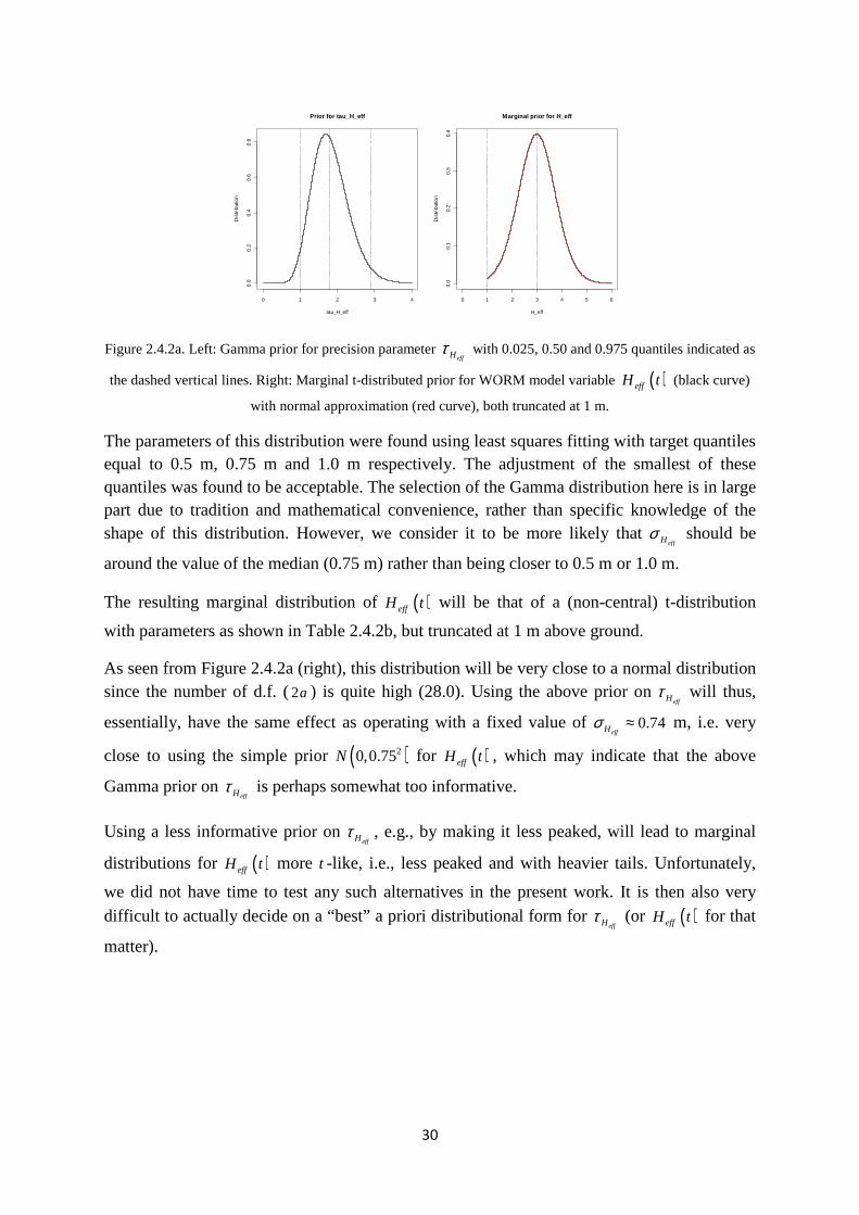
Figure 2.4.2a. Left: Gamma prior for precision parameter effHτ with 0.025, 0.50 and 0.975 quantiles indicated as

the dashed vertical lines. Right: Marginal t-distributed prior for WORM model variable ( )effH t (black curve)

with normal approximation (red curve), both truncated at 1 m.

The parameters of this distribution were found using least squares fitting with target quantiles equal to 0.5 m, 0.75 m and 1.0 m respectively. The adjustment of the smallest of these quantiles was found to be acceptable. The selection of the Gamma distribution here is in large part due to tradition and mathematical convenience, rather than specific knowledge of the shape of this distribution. However, we consider it to be more likely that

effHσ should be

around the value of the median (0.75 m) rather than being closer to 0.5 m or 1.0 m.

The resulting marginal distribution of ( )effH t will be that of a (non-central) t-distribution

with parameters as shown in Table 2.4.2b, but truncated at 1 m above ground.

As seen from Figure 2.4.2a (right), this distribution will be very close to a normal distribution since the number of d.f. (2a ) is quite high (28.0). Using the above prior on

effHτ will thus,

essentially, have the same effect as operating with a fixed value of 0.74effHσ ≈ m, i.e. very

close to using the simple prior ( )20,0.75N for ( )effH t , which may indicate that the above

Gamma prior on effHτ is perhaps somewhat too informative.

Using a less informative prior on effHτ , e.g., by making it less peaked, will lead to marginal

distributions for ( )effH t more t -like, i.e., less peaked and with heavier tails. Unfortunately,

we did not have time to test any such alternatives in the present work. It is then also very difficult to actually decide on a “best” a priori distributional form for

effHτ (or ( )effH t for that

matter).

0 1 2 3 4

0.0

0.2

0.4

0.6

0.8

Prior for tau_H_eff

tau_H_eff

Dis

tribu

tion

0 1 2 3 4 5 6

0.0

0.1

0.2

0.3

0.4

Marginal prior for H_eff

H_eff

Dis

tribu

tion

31

Table 2.4.2b. Prior distributions for model variables of model D.

Variable Marginal distr. D.f 2a

Mean µ Scale

( ) 1/2s ab

−= Approx. distr. Truncation

( )effH t ( )2 ,at sµ 28.0 3.0 m 0.74 m ( )2,N sµ 1 m

( )10mu t ( )2 ,at sµ 15.6 ( )10muf t 0.49 ms-1 ( )2,N sµ 0.1 ms-1

( )10m tϕ ( )2 ,at sµ 15.4 ( )10m

f tϕ 9.8° ( )2,N sµ None

( ),s tη ( )2 ,at sµ 16.8 0 0.46 ( )2,N sµ None

( ),y s tɶ * N/A N/A N/A * None

A tentative uncertainty model for the true hourly average wind speed at 10 m above ground

10mu 9 at time (hour) t is defined as (Tønnesen, 2010; Irwin et al., 2007)

( ) ( ) ( ) ( ) ( ) ( )10 10 10 10

210 10; 0, ; 0.1

m m m mm u u u u mu t f t t t N u tη η σ= + ≥∼ ms-1 (2.4.2b)

where ( )10muf t is the observed hourly average wind speed at time (hour) t at Station 2 .

The precision parameter 10 10

2

m mu uτ σ −= is again given a Gamma distribution with parameters as

shown in Table 2.4.2a, corresponding to a prior distribution on 10muσ with 0.025, 0.50 and

0.975 quantiles equal to 0.36 ms-1, 0.50 ms-1 and 0.75 ms-1 respectively.

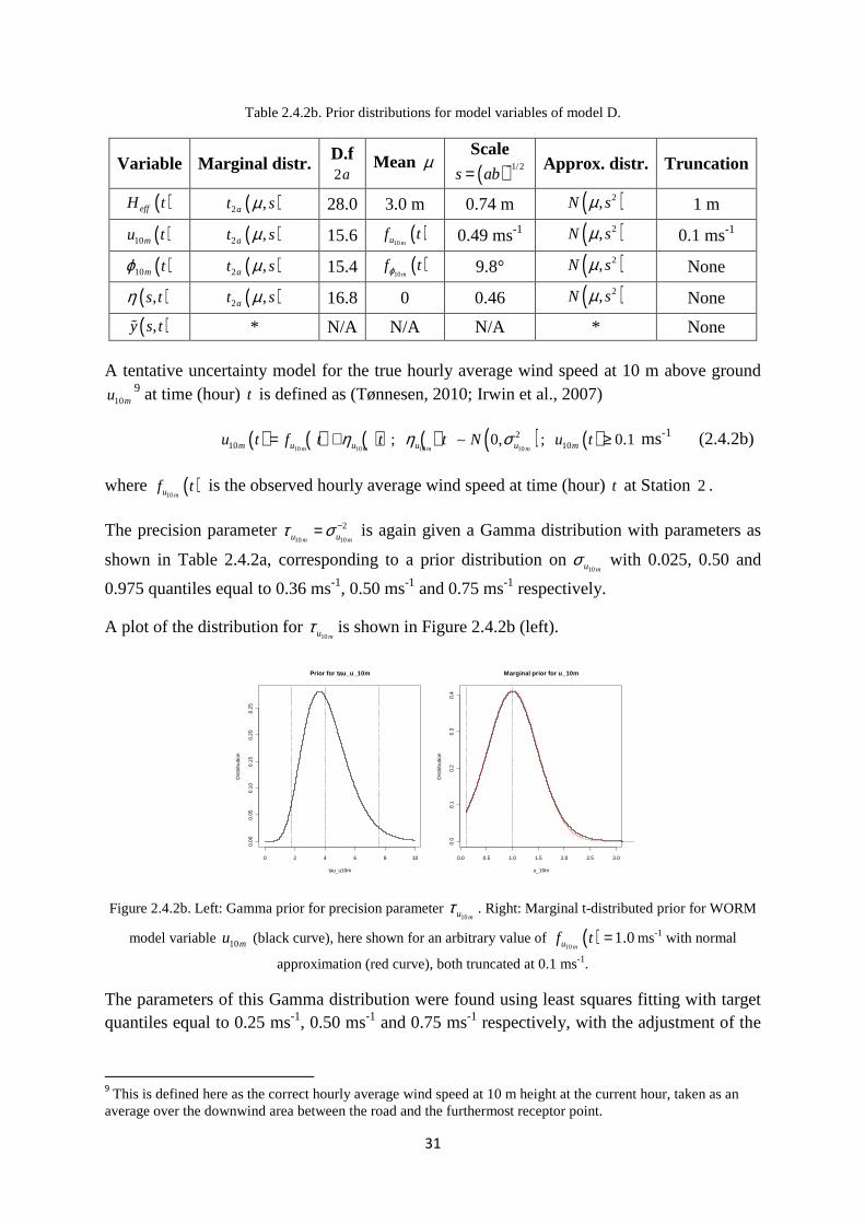
A plot of the distribution for 10muτ is shown in Figure 2.4.2b (left).

Figure 2.4.2b. Left: Gamma prior for precision parameter 10muτ . Right: Marginal t-distributed prior for WORM

model variable 10mu (black curve), here shown for an arbitrary value of ( )10

1.0muf t = ms-1 with normal

approximation (red curve), both truncated at 0.1 ms-1.

The parameters of this Gamma distribution were found using least squares fitting with target quantiles equal to 0.25 ms-1, 0.50 ms-1 and 0.75 ms-1 respectively, with the adjustment of the

9 This is defined here as the correct hourly average wind speed at 10 m height at the current hour, taken as an

average over the downwind area between the road and the furthermost receptor point.

0 2 4 6 8 10

0.00

0.05

0.10

0.15

0.20

0.25

Prior for tau_u_10m

tau_u10m

Dis

tribu

tion

0.0 0.5 1.0 1.5 2.0 2.5 3.0

0.0

0.1

0.2

0.3

0.4

Marginal prior for u_10m

u_10m

Dis

tribu

tion

32

smallest of these quantiles found to be acceptable. The same type of comments that were made regarding the distributional form of

effHτ can also be made here.

The resulting marginal distribution of ( )10mu t , given ( )10muf t , will be that of a (non-central) t-

distribution with parameters as shown in Table 2.4.2b, but truncated at 0.1 m/s. Again, as seen in Figure 2.4.2b (right), the distribution will be close to a truncated normal since the number of d.f. is relatively high (15.6). The same type of comments that were made regarding the distributional form of ( )effH t can also be made here.

A tentative uncertainty model for the true hourly average wind direction at 10 m above ground 10mϕ 10 at time (hour) t is defined as (Tønnesen, 2010; Irwin et al., 2007)

( ) ( ) ( ) ( ) ( )10 10 10 10

210 ; 0,

m m m mm t f t t t Nϕ ϕ ϕ ϕϕ η η σ= + ∼ (2.4.2c)

where ( )10m

f tϕ is the observed hourly average wind direction at time (hour) t at Station 2.

The precision parameter 10 10

2

m mϕ ϕτ σ −= is again given a Gamma distribution with parameters as

shown in Table 2.4.2a, corresponding to a prior distribution on 10mϕσ with 0.025, 0.50 and

0.975 quantiles equal to 7°, 10° and 15° respectively.

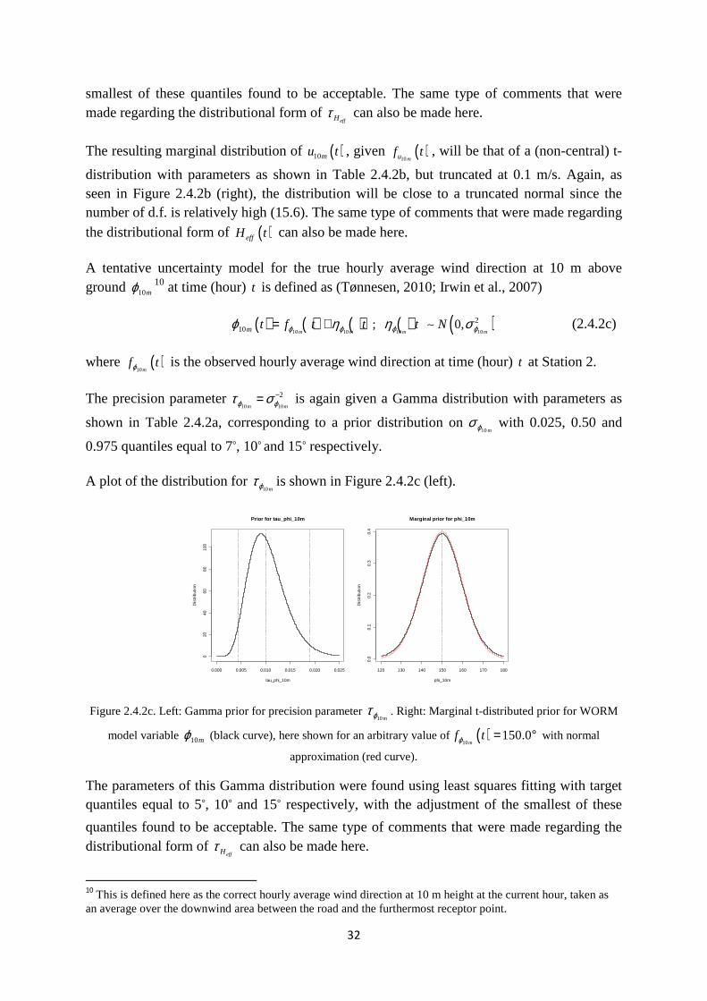
A plot of the distribution for 10mϕτ is shown in Figure 2.4.2c (left).

Figure 2.4.2c. Left: Gamma prior for precision parameter 10mϕτ . Right: Marginal t-distributed prior for WORM

model variable 10mϕ (black curve), here shown for an arbitrary value of ( )10

150.0m

f tϕ = ° with normal

approximation (red curve).

The parameters of this Gamma distribution were found using least squares fitting with target quantiles equal to 5°, 10° and 15° respectively, with the adjustment of the smallest of these

quantiles found to be acceptable. The same type of comments that were made regarding the distributional form of


10

This is defined here as the correct hourly average wind direction at 10 m height at the current hour, taken as an average over the downwind area between the road and the furthermost receptor point.

0.000 0.005 0.010 0.015 0.020 0.025

020

4060

8010

0

Prior for tau_phi_10m

tau_phi_10m

Dis

tribu

tion

120 130 140 150 160 170 180

0.0

0.1

0.2

0.3

0.4

Marginal prior for phi_10m

phi_10m

Dis

tribu

tion

33

The resulting marginal distribution of ( )10m tϕ given ( )10m

f tϕ will be a (non-central) t-

distribution with parameters as shown in Table 2.4.2b. Again, as seen in Figure 2.4.2c, the distribution will be close to a normal since the number of d.f. is relatively high (15.4). The same type of comments that were made regarding the distributional form of ( )effH t can also

be made here.

The above prior distributions for ( )effH t , ( )10mu t and ( )10m tϕ are assumed to be independent.

Ideally here, we should have included dependency modelling between wind speed and wind direction since clearly the uncertainty in wind direction increases with decreasing wind speed. However, since the above prior model for uncertainty in wind direction is actually oriented towards low wind speeds, we have, as a first approximation, defined the priors here to be independent. Even though this will result in wind directions being somewhat too uncertain in situations with strong wind, concentrations will then be much lower, so the consequences of this approximation on uncertainty in concentration will not be so severe.

A tentative uncertainty model for the hourly average predictive concentration ( ),y s tɶ at an

arbitrary spatial location s and time (hour) t , given true values of ( )effH t , ( )10mu t and ( )10m tϕ

is defined as

( ) ( ) ( ) ( )( ) ( ) ( ) ( )210 10log , log , , , , , ; , 0,c eff m my s t f s t H t u t t s t s t Nϕ η η σ= +ɶ ∼ (2.4.2d)

where ( ) ( ) ( )( )10 10, , , ,c eff m mf s t H t u t tϕ is the hourly average concentration calculated with the

WORM model at the same space and time locations using true input values of the WORM

model variables ( )effH t , ( )10mu t and ( )10m tϕ .

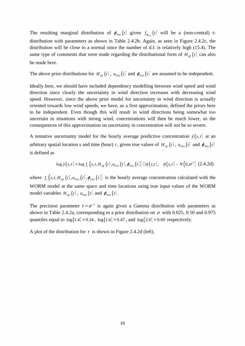
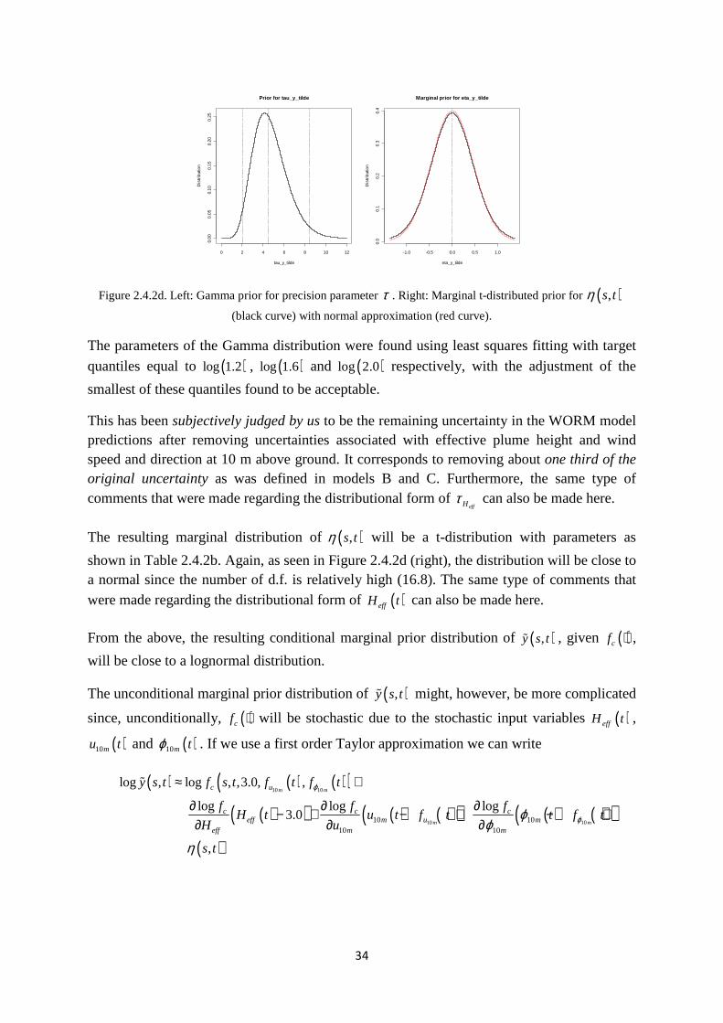
The precision parameter 2τ σ −= is again given a Gamma distribution with parameters as shown in Table 2.4.2a, corresponding to a prior distribution on σ with 0.025, 0.50 and 0.975 quantiles equal to ( )log 1.4 0.34≈ , ( )log 1.6 0.47≈ , and ( )log 2.0 0.69≈ respectively.

A plot of the distribution for τ is shown in Figure 2.4.2d (left).

34

Figure 2.4.2d. Left: Gamma prior for precision parameter τ . Right: Marginal t-distributed prior for ( ),s tη

(black curve) with normal approximation (red curve).

The parameters of the Gamma distribution were found using least squares fitting with target

quantiles equal to ( )log 1.2 , ( )log 1.6 and ( )log 2.0 respectively, with the adjustment of the

smallest of these quantiles found to be acceptable.

This has been subjectively judged by us to be the remaining uncertainty in the WORM model predictions after removing uncertainties associated with effective plume height and wind speed and direction at 10 m above ground. It corresponds to removing about one third of the original uncertainty as was defined in models B and C. Furthermore, the same type of comments that were made regarding the distributional form of


The resulting marginal distribution of ( ),s tη will be a t-distribution with parameters as

shown in Table 2.4.2b. Again, as seen in Figure 2.4.2d (right), the distribution will be close to a normal since the number of d.f. is relatively high (16.8). The same type of comments that were made regarding the distributional form of ( )effH t can also be made here.

From the above, the resulting conditional marginal prior distribution of ( ),y s tɶ , given ( )cf ⋅ ,

will be close to a lognormal distribution.

The unconditional marginal prior distribution of ( ),y s tɶ might, however, be more complicated

since, unconditionally, ( )cf ⋅ will be stochastic due to the stochastic input variables ( )effH t ,

( )10mu t and ( )10m tϕ . If we use a first order Taylor approximation we can write

( ) ( ) ( )( )( )( ) ( ) ( )( ) ( ) ( )( )

( )

10 10

10 1010 1010 10

log , log , ,3.0, ,

log log log 3.0

,

m m

m m

c u

c c ceff m u m

eff m m

y s t f s t f t f t

f f fH t u t f t t f t

H u

s t

ϕ

ϕϕϕ

η

≈ +

∂ ∂ ∂− + − + − +

∂ ∂ ∂

ɶ

0 2 4 6 8 10 12

0.00

0.05

0.10

0.15

0.20

0.25

Prior for tau_y_tilde

tau_y_tilde

Dis

tribu

tion

-1.0 -0.5 0.0 0.5 1.0

0.0

0.1

0.2

0.3

0.4

Marginal prior for eta_y_tilde

eta_y_tilde

Dis

tribu

tion

35

and since ( )effH t , ( )10mu t and ( )10m tϕ are all approximately normally distributed, as shown in

Figures 2.4.2a-c, ( )log ,y s tɶ will also be approximately normal, with the following first and

second order moments:

( ) ( ) ( )( )10 10

log , log , ,3.0, ,m mc uE y s t f s t f t f tϕ≈ɶ

and

( )10 10

2 2 2

2 2 2 2

10 10

log log logvar log ,

eff m m

c c cH u

eff m m

f f fy s t

H u ϕσ σ σ σϕ

∂ ∂ ∂≈ + + + ∂ ∂ ∂

ɶ

where effHσ ,

10muσ and 10mϕσ are given by the scale values in Table 2.4.2b, 0.47σ ≈ , and

where the partial derivatives will vary with time (hour) t .

Hence, ( ),y s tɶ will also be approximately lognormally distributed with median

( ) ( )( )10 10

, ,3.0, ,m mc uf s t f t f tϕ

and with geometrical standard deviation

( )( )10 10

2 2 2

2 2 2 2

10 10

log log log, exp

eff m m

c c cg H u

eff m m

f f fSD y s t

H u ϕσ σ σ σϕ

∂ ∂ ∂ ≈ + + + ∂ ∂ ∂

ɶ . (2.4.2e)

Thus, geometrical standard deviations of predictive distributions from model D will, according to (2.4.2e), dynamically vary with time depending on the numerical values of the partial derivatives (associated with model sensitivity), and variances of the model variables involved.

For example, partial derivatives with respect to wind speed will be higher when the wind speed is low than when it is high, since the model is more sensitive to changes in the wind speed when the wind speed is lower. Likewise, partial derivatives with respect to wind direction will be higher when the wind direction is almost parallel to the road than in a situation where the wind direction is more perpendicular on the road. The partial derivatives with respect to effective plume height will vary with the meteorological conditions and also with the transport time of the plume from source to receptor.

Predictive distributions from model D might therefore be sharper than predictive distributions from other non-hierarchical models, such as e.g., models A-C, but this then depends on the accuracies of the partial derivatives (which again depends on the accuracy of the WORM model), and on how accurate the variances of the three WORM model variables and the residual have been specified.

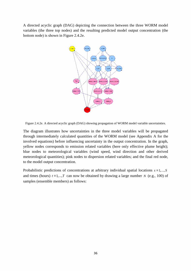
A directed acyclic graph (DAG) depictingvariables (the three top nodes) bottom node) is shown in Figure 2.4.2e.

Figure 2.4.2e. A directed acyclic graph (DAG) showing

The diagram illustrates how through intermediately calculated quantities ofinvolved equations) before influencing uncertainty in yellow nodes corresponds to blue nodes to meteorological variablesmeteorological quantities); pink nodes to the model output concentration.

Probabilistic predictions of concentrations

and times (hours) 1,...,t T= can now be obtained by drawing a large number

samples (ensemble members)

36

clic graph (DAG) depicting the connection between the three(the three top nodes) and the resulting predicted model output concentration

is shown in Figure 2.4.2e.

ic graph (DAG) showing propagation of WORM model variable uncertainties.

how uncertainties in the three model variables will becalculated quantities of the WORM model (see Appendix A for

nfluencing uncertainty in the output concentration emission related variables (here only effective plume height)

logical variables (wind speed, wind direction andpink nodes to dispersion related variables; and

concentration.

of concentrations at arbitrary individual spatial locations

can now be obtained by drawing a large number

as follows:

three WORM model and the resulting predicted model output concentration (the

model variable uncertainties.

variables will be propagated RM model (see Appendix A for the

output concentration. In the graph, effective plume height);

(wind speed, wind direction and other derived dispersion related variables; and the final red node,

ary individual spatial locations 1,...,s S=

can now be obtained by drawing a large number N (e.g., 100) of

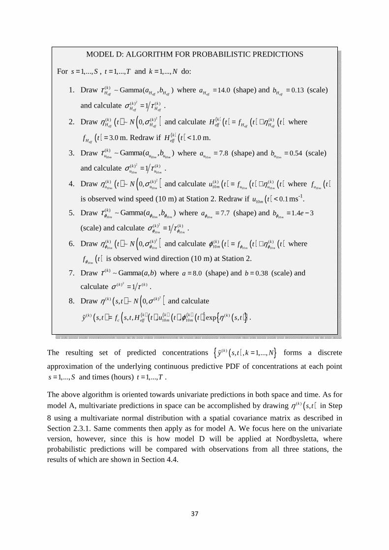
37



The above algorithm is oriented towards univariate predictions in both space and time. As for

model A, multivariate predictions in space can be accomplished by drawing ( )( ) ,k s tη in Step

8 using a multivariate normal distribution with a spatial covariance matrix as described in Section 2.3.1. Same comments then apply as for model A. We focus here on the univariate version, however, since this is how model D will be applied at Nordbysletta, where probabilistic predictions will be compared with observations from all three stations, the results of which are shown in Section 4.4.

MODEL D: ALGORITHM FOR PROBABILISTIC PREDICTIONS

For 1,...,s S= , 1,...,t T= and 1,...,k N= do:

1. Draw ( ) Gamma( , )eff eff eff

kH H Ha bτ ∼ where 14.0

effHa = (shape) and 0.13effHb = (scale)

and calculate 2( ) ( )1

eff eff

k kH Hσ τ= .

2. Draw ( ) ( )2( ) ( )0,eff eff

k kH Ht Nη σ∼ and calculate ( ) ( ) ( ) ( )( )

eff eff

k keff H HH t f t tη= + where

( ) 3.0effHf t = m. Redraw if ( ) ( ) 1.0k

effH t < m.

3. Draw 10 10 10

( ) Gamma( , )m m m

ku u ua bτ ∼ where

107.8

mua = (shape) and 10

0.54mub = (scale)

and calculate 2

10 10

( ) ( )1m m

k ku uσ τ= .

4. Draw ( ) ( )2

10 10

( ) ( )0,m m

k ku ut Nη σ∼ and calculate ( ) ( ) ( )

10 10

( ) ( )10 m m

k km u uu t f t tη= + where ( )

10muf t

is observed wind speed (10 m) at Station 2. Redraw if ( )10 0.1mu t < ms-1.

5. Draw 10 10 10

( ) Gamma( , )m m m

k a bϕ ϕ ϕτ ∼ where 10

7.7m

aϕ = (shape) and 10

1.4 3m

b eϕ = −

(scale) and calculate 2

10 10

( ) ( )1m m

k kϕ ϕσ τ= .

6. Draw ( ) ( )2

10 10

( ) ( )0,m m

k kt Nϕ ϕη σ∼ and calculate ( ) ( ) ( )10 10

( ) ( )10 m m

k km t f t tϕ ϕϕ η= + where

( )10m

f tϕ is observed wind direction (10 m) at Station 2.

7. Draw ( ) Gamma( , )k a bτ ∼ where 8.0a = (shape) and 0.38b = (scale) and

calculate 2( ) ( )1k kσ τ= .

8. Draw ( ) ( )2( ) ( ), 0,k ks t Nη σ∼ and calculate

( ) ( ) ( ) ( ) ( ) ( ) ( )( ) ( ) ( ) ( )10 10, , , , , exp ,k k kk k

c eff m my s t f s t H t u t t s tϕ η=ɶ .

39

3. METHODOLOGIES

In this chapter we describe some statistical methodologies that are used to produce most of the results in Chapter 4. First in Sections 3.1 and 3.2 we describe some tools and measures which are used to evaluate and characterize the performance of probabilistic predictions made by the models A-D as compared with observations. In Section 3.3 we review the Metropolis-within-Gibbs sampling algorithm as this is used as part of model C to produce posterior distributions of the parameters in this model. Section 3.4 shortly reviews circular block bootstrapping since this is used as a technique to preserve the dependence structure of the time-series of observed and model calculated values which is important for the proper bootstrap calculation of some of the measures introduced in Sections 3.1-2.

3.1 Calibration and sharpness of predictive distributions11

We review the concepts of calibration and sharpness of predictive distributions of continuous variables as defined and discussed in Gneiting et al. (2007a). These issues are central and important for evaluating performance of probabilistic predictions of continuous variables.

These concepts form part of the much broader field of forecast verification, which have been evolved, especially in the meteorological communities, over the past decades. The book by Joliffe and Stephenson (2003), and Chapters 6-7 in Wilks (2006), provide a good exposition of this rapidly growing field. An excellent and recent survey of the state-of-the-science in verification practice, research and development, is given in Casati et al. (2008).

Calibration is associated with the statistical consistency between predictive distributions and accompanying observations, and is thus a common property of these. Sharpness refers to spread or width of the predictive distributions only and is, therefore, not dependent on any observations. The spread can e.g., be measured using standard deviation, or 50% or 90% central interval widths.

According to Gneiting et al. (2007a) we may distinguish between three types of calibration:

1. Probabilistic (or time) calibration 2. Exceedance calibration 3. Marginal calibration

A system is probabilistically calibrated if observations are virtually indistinguishable from samples taken from the predictive distributions, which means that the rank or PIT (Probability Integral Transform) histograms as defined below will have a uniform appearance. A system is exceedance calibrated if there is a consistency between predicted and

11

This text draws heavily on Gneiting et al. (2007a), including use of part of phrases, description of concepts, stated definitions and theorems.

40

observed thresholds. Finally, a system is marginally calibrated if predictions and observations as taken over time have the same (or nearly the same) marginal distribution.

We will first formally define these concepts before describing diagnostic tools for evaluation using sample based distributions.

Let the predictive distributions be denoted by tF , and the outcomes (observations) be denoted

by ty , for a sequence of time instances 1,2,...,t T= , where the observations are thought to be

generated by some underlying true (but unknown) data generating process with distributions

tG , 1,2,...,t T= . The asymptotic compliance between the data generating process tG and the

predictive distributions tF will now be defined in terms of the above three main types of

calibration. Since the distribution may depend on parameters being stochastic, convergence is here defined in terms of almost sure convergence as T → ∞ .

Definition 3.1a (types of calibration).

1. The sequence ( )tF , 1,2,...t = is probabilistically calibrated relative to the sequence

( )tG , 1,2,...t = if

( ) ( )1

1

1 for all 0,1 .

T

t tt

G F p p pT

−

=

→ ∈∑

2. The sequence ( )tF , 1,2,...t = is exceedance calibrated relative to the sequence ( )tG ,

1,2,...t = if

( )1

1

1 for all y .

T

t tt

G F y yT

−

=

→ ∈∑ ℝ

3. The sequence ( )tF , 1,2,...t = is marginally calibrated relative to ( )tG , 1,2,...t = if the

limits

( ) ( )1

1lim

T

tTt

G y G yT→∞ =

= ∑

and

( ) ( )1

1lim

T

tTt

F y F yT→∞ =

= ∑

exists and are equal for all y∈ℝ , and if the common limit distribution has all its mass

on a finite volume.

4. The sequence ( )tF , 1,2,...t = is strongly calibrated relative to ( )tG , 1,2,...t = if it is

probabilistically calibrated, exceedance calibrated and marginally calibrated.

41

In Gneiting et al. (2007a) it is shown that the first three types of calibration are logically independent and that they may occur in any combination. The existence of the marginal

distribution G associated with the true data generating process, corresponds to the existence of a stable climate over time. In our context of air pollution modelling it corresponds to a stable, long term average pattern regarding local emissions and meteorological conditions.

We now turn to sample versions of the above definitions by using empirical distribution functions based on observations. In Gneiting et al. (2007a) sample based analogues to the above definitions are provided for probabilistic and marginal calibration, which will be described below. Exceedance calibration, however, does not seem to have an obvious sample analogue, and it is not known whether such an analogue exists (Gneiting et al. 2007a). We will, therefore, not pursue the concept of exceedance calibration any further here.

Assessing probabilistic calibration.

As stated above, probabilistic calibration can be assessed by the PIT-histogram. The PIT-histogram can be viewed as a continuous limit of the rank histogram (also known as the Talagrand diagram), as defined in e.g., Wilks (2006) or Joliffe and Stephenson (2003).

The PIT is the value of the predictive CDF (tF ) at the observation (ty ), i.e., the value

( )t t tp F y= . The link to probabilistic calibration is established by substituting the empirical

indicator function ( )1 ty y≤ for the data generating distribution ( )tG y , y∈ℝ , in the

probabilistic calibration condition, and noting that ( )1t ty F p−≤ if and only if tp p≤ . The

following theorem links probabilistic calibration with the asymptotic uniformity of an empirical sequence of PIT-values.

Theorem 3.1a. Let ( )tF , 1,2,...t = and ( )tG , 1,2,...t = be sequences of continuous strictly

increasing distribution functions. Suppose further that ty has distribution tG and that ty form

a “*-mixing” sequence of random variables (Blum et al, 1963). Then

( )1

11 almost surely for all

T

tt

p p p pT =

≤ →∑

if and only if ( )tF , 1,2,...t = is probabilistically calibrated with respect to ( )tG , 1,2,...t = .

For a proof of this theorem, see Gneiting et al. (2007a).

Thus for a probabilistically well-calibrated system, histograms of PIT-values, will essentially be uniform or close to uniform. The number of bins to be used in the histograms will depend on the application and amount of data available, but for most purposes, however, 10-20 bins seem to be sufficient (Gneiting et al., 2007a).

Another measure associated with probabilistic calibration, but weaker, is the concept of central interval coverage. If we e.g., calculate the 50% or 90% central intervals for each predictive distribution, observations should appear in these intervals around 50% or 90% of the time, respectively, if the system is well-calibrated. Even though this is a weaker (less

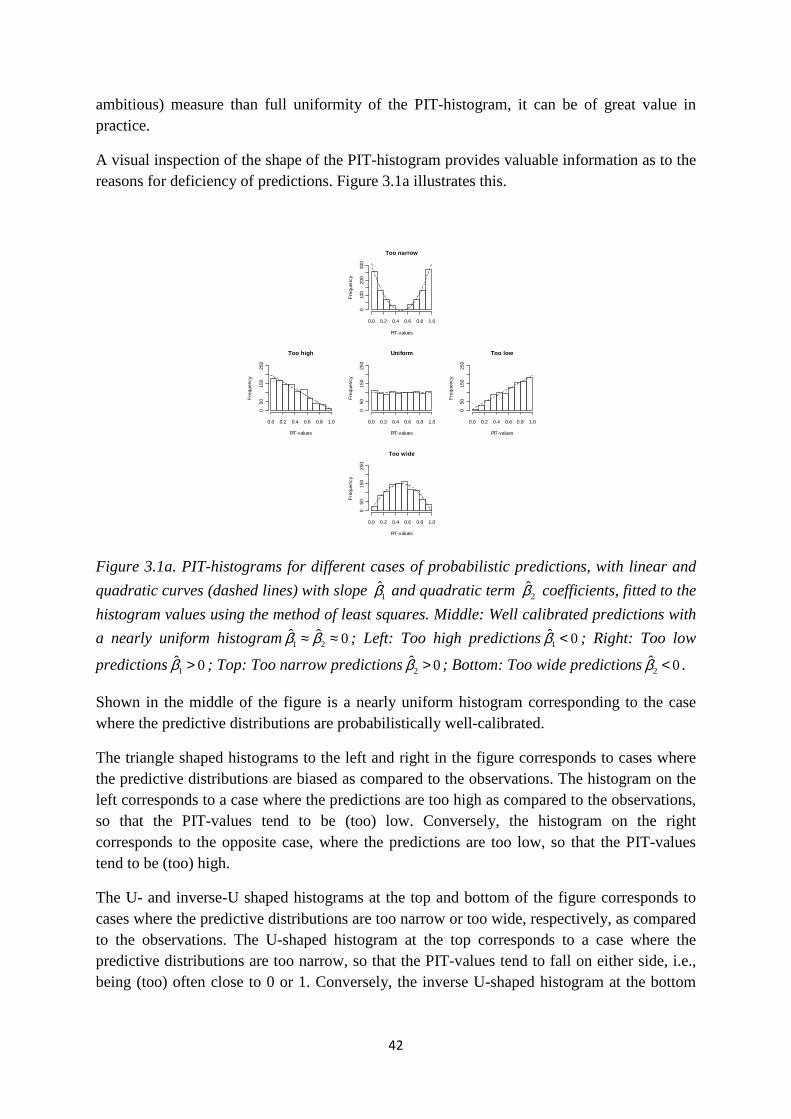
42

ambitious) measure than full uniformity of the PIT-histogram, it can be of great value in practice.

A visual inspection of the shape of the PIT-histogram provides valuable information as to the reasons for deficiency of predictions. Figure 3.1a illustrates this.

Figure 3.1a. PIT-histograms for different cases of probabilistic predictions, with linear and

quadratic curves (dashed lines) with slope 1β and quadratic term 2β coefficients, fitted to the

histogram values using the method of least squares. Middle: Well calibrated predictions with

a nearly uniform histogram1 2ˆ ˆ 0β β≈ ≈ ; Left: Too high predictions1 0β < ; Right: Too low

predictions 1 0β > ; Top: Too narrow predictions2ˆ 0β > ; Bottom: Too wide predictions2ˆ 0β < .

Shown in the middle of the figure is a nearly uniform histogram corresponding to the case where the predictive distributions are probabilistically well-calibrated.

The triangle shaped histograms to the left and right in the figure corresponds to cases where the predictive distributions are biased as compared to the observations. The histogram on the left corresponds to a case where the predictions are too high as compared to the observations, so that the PIT-values tend to be (too) low. Conversely, the histogram on the right corresponds to the opposite case, where the predictions are too low, so that the PIT-values tend to be (too) high.

The U- and inverse-U shaped histograms at the top and bottom of the figure corresponds to cases where the predictive distributions are too narrow or too wide, respectively, as compared to the observations. The U-shaped histogram at the top corresponds to a case where the predictive distributions are too narrow, so that the PIT-values tend to fall on either side, i.e., being (too) often close to 0 or 1. Conversely, the inverse U-shaped histogram at the bottom

Too high

PIT-values

Fre

quen

cy

0.0 0.2 0.4 0.6 0.8 1.0

050

150

250

Uniform

PIT-values

Fre

quen

cy

0.0 0.2 0.4 0.6 0.8 1.0

050

150

250

Too low

PIT-values

Fre

quen

cy

0.0 0.2 0.4 0.6 0.8 1.0

050

150

250

Too wide

PIT-values

Fre

quen

cy

0.0 0.2 0.4 0.6 0.8 1.0

050

150

250

Too narrow

PIT-values

Fre

quen

cy

0.0 0.2 0.4 0.6 0.8 1.0

010

020

030

0

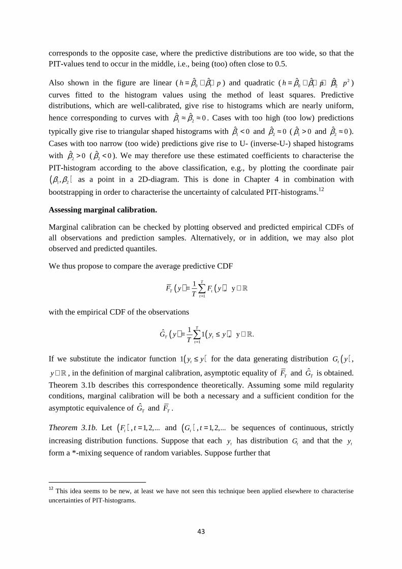
43

corresponds to the opposite case, where the predictive distributions are too wide, so that the PIT-values tend to occur in the middle, i.e., being (too) often close to 0.5.

Also shown in the figure are linear ( 0 1ˆ ˆh pβ β= + ⋅ ) and quadratic ( 2

0 1 2ˆ ˆ ˆh p pβ β β= + ⋅ + ⋅ )

curves fitted to the histogram values using the method of least squares. Predictive distributions, which are well-calibrated, give rise to histograms which are nearly uniform,

hence corresponding to curves with 1 2ˆ ˆ 0β β≈ ≈ . Cases with too high (too low) predictions

typically give rise to triangular shaped histograms with 1 0β < and 2ˆ 0β ≈ ( 1 0β > and 2

ˆ 0β ≈ ).

Cases with too narrow (too wide) predictions give rise to U- (inverse-U-) shaped histograms

with 2ˆ 0β > ( 2

ˆ 0β < ). We may therefore use these estimated coefficients to characterise the

PIT-histogram according to the above classification, e.g., by plotting the coordinate pair

( )1 2,β β as a point in a 2D-diagram. This is done in Chapter 4 in combination with

bootstrapping in order to characterise the uncertainty of calculated PIT-histograms.12

Assessing marginal calibration.

Marginal calibration can be checked by plotting observed and predicted empirical CDFs of all observations and prediction samples. Alternatively, or in addition, we may also plot observed and predicted quantiles.

We thus propose to compare the average predictive CDF

( ) ( )1

1, y

T

T tt

F y F yT =

= ∈∑ ℝ

with the empirical CDF of the observations

( ) ( )1

1ˆ 1 , y .T

T tt

G y y yT =

= ≤ ∈∑ ℝ

If we substitute the indicator function ( )1 ty y≤ for the data generating distribution ( )tG y ,

y∈ℝ , in the definition of marginal calibration, asymptotic equality of TF and ˆTG is obtained.

Theorem 3.1b describes this correspondence theoretically. Assuming some mild regularity conditions, marginal calibration will be both a necessary and a sufficient condition for the

asymptotic equivalence of ˆTG and TF .

Theorem 3.1b. Let ( )tF , 1,2,...t = and ( )tG , 1,2,...t = be sequences of continuous, strictly

increasing distribution functions. Suppose that each ty has distribution tG and that the ty form a *-mixing sequence of random variables. Suppose further that

12

This idea seems to be new, at least we have not seen this technique been applied elsewhere to characterise uncertainties of PIT-histograms.

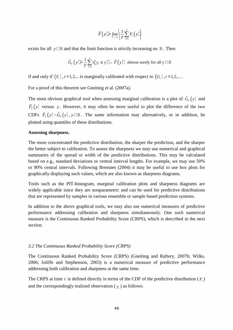
44

( ) ( )1

1lim

T

tTt

F y F yT→∞ =

= ∑

exists for all y∈ℝ and that the limit function is strictly increasing on ℝ . Then

( ) ( ) ( )1

1ˆ 1 almost surely for all yT

T tt

G y y y F yT =

= ≤ → ∈∑ ℝ

if and only if ( )tF , 1,2,...t = is marginally calibrated with respect to ( )tG , 1,2,...t = .

For a proof of this theorem see Gneiting et al. (2007a).

The most obvious graphical tool when assessing marginal calibration is a plot of ( )ˆTG y and

( )TF y versus y . However, it may often be more useful to plot the difference of the two

CDFs ( ) ( )ˆT TF y G y− , y∈ℝ . The same information may alternatively, or in addition, be

plotted using quantiles of these distributions.

Assessing sharpness.

The more concentrated the predictive distribution, the sharper the prediction, and the sharper the better subject to calibration. To assess the sharpness we may use numerical and graphical summaries of the spread or width of the predictive distributions. This may be calculated based on e.g., standard deviations or central interval lengths. For example, we may use 50% or 90% central intervals. Following Bremnes (2004) it may be useful to use box plots for graphically displaying such values, which are also known as sharpness diagrams.

Tools such as the PIT-histogram, marginal calibration plots and sharpness diagrams are widely applicable since they are nonparametric and can be used for predictive distributions that are represented by samples in various ensemble or sample based prediction systems.

In addition to the above graphical tools, we may also use numerical measures of predictive performance addressing calibration and sharpness simultaneously. One such numerical measure is the Continuous Ranked Probability Score (CRPS), which is described in the next section.

3.2 The Continuous Ranked Probability Score (CRPS)

The Continuous Ranked Probability Score (CRPS) (Gneiting and Raftery, 2007b; Wilks, 2006; Joliffe and Stephenson, 2003) is a numerical measure of predictive performance addressing both calibration and sharpness at the same time.

The CRPS at time t is defined directly in terms of the CDF of the predictive distribution ( tF )

and the correspondingly realized observation (ty ) as follows:

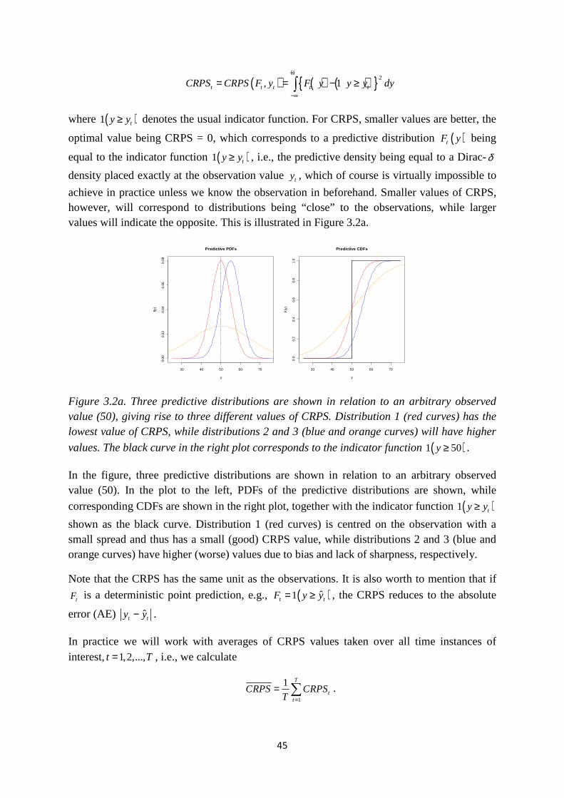
45

( ) ( ) ( ) 2, 1t t t t tCRPS CRPS F y F y y y dy

+∞

−∞

= = − ≥∫

where ( )1 ty y≥ denotes the usual indicator function. For CRPS, smaller values are better, the

optimal value being CRPS = 0, which corresponds to a predictive distribution ( )tF y being

equal to the indicator function ( )1 ty y≥ , i.e., the predictive density being equal to a Dirac-δ

density placed exactly at the observation value ty , which of course is virtually impossible to

achieve in practice unless we know the observation in beforehand. Smaller values of CRPS, however, will correspond to distributions being “close” to the observations, while larger values will indicate the opposite. This is illustrated in Figure 3.2a.

Figure 3.2a. Three predictive distributions are shown in relation to an arbitrary observed value (50), giving rise to three different values of CRPS. Distribution 1 (red curves) has the lowest value of CRPS, while distributions 2 and 3 (blue and orange curves) will have higher

values. The black curve in the right plot corresponds to the indicator function ( )1 50y ≥ .

In the figure, three predictive distributions are shown in relation to an arbitrary observed value (50). In the plot to the left, PDFs of the predictive distributions are shown, while

corresponding CDFs are shown in the right plot, together with the indicator function ( )1 ty y≥

shown as the black curve. Distribution 1 (red curves) is centred on the observation with a small spread and thus has a small (good) CRPS value, while distributions 2 and 3 (blue and orange curves) have higher (worse) values due to bias and lack of sharpness, respectively.

Note that the CRPS has the same unit as the observations. It is also worth to mention that if

tF is a deterministic point prediction, e.g., ( )ˆ1t tF y y= ≥ , the CRPS reduces to the absolute

error (AE) ˆt ty y− .

In practice we will work with averages of CRPS values taken over all time instances of interest, 1,2,...,t T= , i.e., we calculate

1

1 T

tt

CRPS CRPST =

= ∑ .

30 40 50 60 70

0.00

0.02

0.04

0.06

0.08

Predictive PDFs

y

f(y)

30 40 50 60 70

0.0

0.2

0.4

0.6

0.8

1.0

Predictive CDFs

y

F(y

)

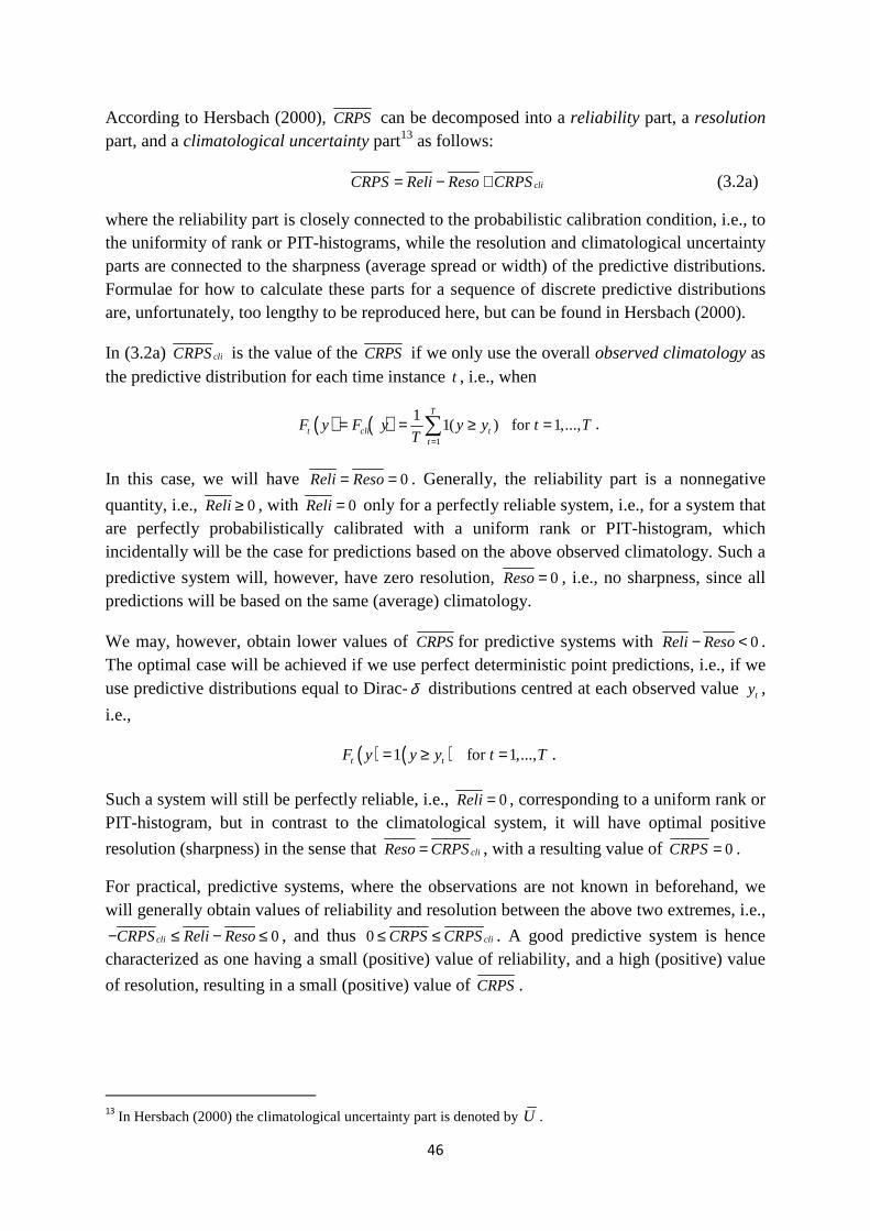
46

According to Hersbach (2000), CRPS can be decomposed into a reliability part, a resolution part, and a climatological uncertainty part13 as follows:

cliCRPS Reli Reso CRPS= − + (3.2a)

where the reliability part is closely connected to the probabilistic calibration condition, i.e., to the uniformity of rank or PIT-histograms, while the resolution and climatological uncertainty parts are connected to the sharpness (average spread or width) of the predictive distributions. Formulae for how to calculate these parts for a sequence of discrete predictive distributions are, unfortunately, too lengthy to be reproduced here, but can be found in Hersbach (2000).

In (3.2a) cliCRPS is the value of the CRPS if we only use the overall observed climatology as the predictive distribution for each time instance t , i.e., when

( ) ( )1

11( ) for 1,...,

T

t cli tt

F y F y y y t TT =

= = ≥ =∑ .

In this case, we will have 0Reli Reso= = . Generally, the reliability part is a nonnegative

quantity, i.e., 0Reli≥ , with 0Reli = only for a perfectly reliable system, i.e., for a system that are perfectly probabilistically calibrated with a uniform rank or PIT-histogram, which incidentally will be the case for predictions based on the above observed climatology. Such a

predictive system will, however, have zero resolution, 0Reso= , i.e., no sharpness, since all predictions will be based on the same (average) climatology.

We may, however, obtain lower values of CRPSfor predictive systems with 0Reli Reso− < . The optimal case will be achieved if we use perfect deterministic point predictions, i.e., if we use predictive distributions equal to Dirac-δ distributions centred at each observed value ty ,

i.e.,

( ) ( )1 for 1,...,t tF y y y t T= ≥ = .

Such a system will still be perfectly reliable, i.e., 0Reli = , corresponding to a uniform rank or PIT-histogram, but in contrast to the climatological system, it will have optimal positive

resolution (sharpness) in the sense that cliReso CRPS= , with a resulting value of 0CRPS= .

For practical, predictive systems, where the observations are not known in beforehand, we will generally obtain values of reliability and resolution between the above two extremes, i.e.,

0cliCRPS Reli Reso− ≤ − ≤ , and thus 0 cliCRPS CRPS≤ ≤ . A good predictive system is hence characterized as one having a small (positive) value of reliability, and a high (positive) value

of resolution, resulting in a small (positive) value of CRPS.

13 In Hersbach (2000) the climatological uncertainty part is denoted by U .

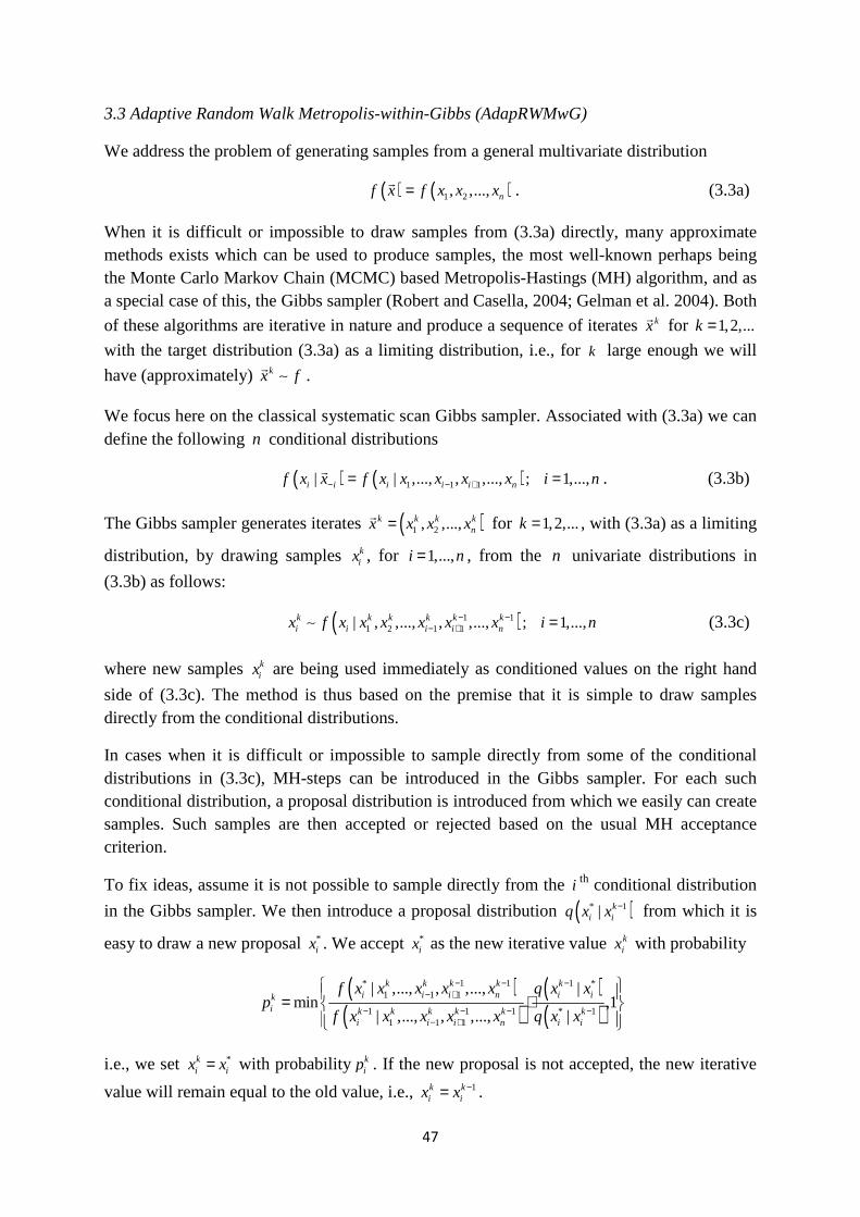
47

3.3 Adaptive Random Walk Metropolis-within-Gibbs (AdapRWMwG)

We address the problem of generating samples from a general multivariate distribution

( ) ( )1 2, ,..., nf x f x x x= . (3.3a)

When it is difficult or impossible to draw samples from (3.3a) directly, many approximate methods exists which can be used to produce samples, the most well-known perhaps being the Monte Carlo Markov Chain (MCMC) based Metropolis-Hastings (MH) algorithm, and as a special case of this, the Gibbs sampler (Robert and Casella, 2004; Gelman et al. 2004). Both

of these algorithms are iterative in nature and produce a sequence of iterates kx

for 1,2,...k =

with the target distribution (3.3a) as a limiting distribution, i.e., for k large enough we will

have (approximately) kx f∼ .

We focus here on the classical systematic scan Gibbs sampler. Associated with (3.3a) we can define the following n conditional distributions

( ) ( )1 1 1| | ,..., , ,..., ; 1,...,i i i i i nf x x f x x x x x i n− − += =. (3.3b)

The Gibbs sampler generates iterates ( )1 2, ,...,k k k knx x x x= for 1,2,...k = , with (3.3a) as a limiting

distribution, by drawing samples kix , for 1,...,i n= , from the n univariate distributions in

(3.3b) as follows:

( )1 11 2 1 1| , ,..., , ,..., ; 1,...,k k k k k k

i i i i nx f x x x x x x i n− −− + =∼ (3.3c)

where new samples kix are being used immediately as conditioned values on the right hand

side of (3.3c). The method is thus based on the premise that it is simple to draw samples directly from the conditional distributions.

In cases when it is difficult or impossible to sample directly from some of the conditional distributions in (3.3c), MH-steps can be introduced in the Gibbs sampler. For each such conditional distribution, a proposal distribution is introduced from which we easily can create samples. Such samples are then accepted or rejected based on the usual MH acceptance criterion.

To fix ideas, assume it is not possible to sample directly from the i th conditional distribution

in the Gibbs sampler. We then introduce a proposal distribution ( )* 1| ki iq x x − from which it is

easy to draw a new proposal *ix . We accept *

ix as the new iterative value kix with probability

( )

( )( )( )

* 1 1 1 *1 1 1

1 1 1 * 11 1 1

| ,..., , ,..., |min ,1

| ,..., , ,..., |

k k k k ki i i n i ik

i k k k k k ki i i n i i

f x x x x x q x xp

f x x x x x q x x

− − −− +

− − − −− +

= ⋅

i.e., we set *ki ix x= with probability k

ip . If the new proposal is not accepted, the new iterative

value will remain equal to the old value, i.e., 1k ki ix x −= .

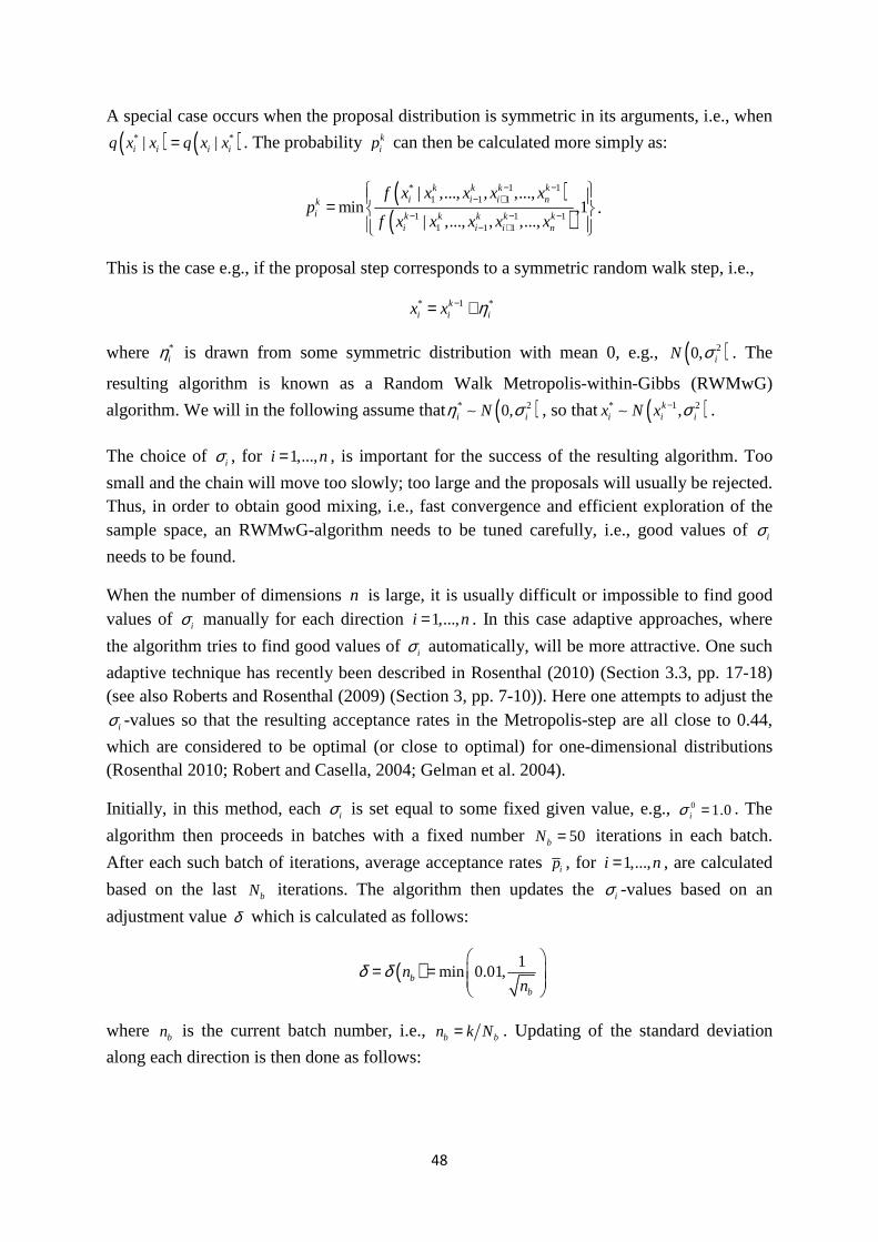
48

A special case occurs when the proposal distribution is symmetric in its arguments, i.e., when

( ) ( )* *| |i i i iq x x q x x= . The probability kip can then be calculated more simply as:

( )

( )* 1 1

1 1 1

1 1 11 1 1

| ,..., , ,...,min ,1

| ,..., , ,...,

k k k ki i i nk

i k k k k ki i i n

f x x x x xp

f x x x x x

− −− +

− − −− +

=

.

This is the case e.g., if the proposal step corresponds to a symmetric random walk step, i.e.,

* 1 *ki i ix x η−= +

where *iη is drawn from some symmetric distribution with mean 0, e.g., ( )20, iN σ . The

resulting algorithm is known as a Random Walk Metropolis-within-Gibbs (RWMwG)

algorithm. We will in the following assume that ( )* 20,i iNη σ∼ , so that ( )* 1 2,ki i ix N x σ−∼ .

The choice of iσ , for 1,...,i n= , is important for the success of the resulting algorithm. Too

small and the chain will move too slowly; too large and the proposals will usually be rejected. Thus, in order to obtain good mixing, i.e., fast convergence and efficient exploration of the sample space, an RWMwG-algorithm needs to be tuned carefully, i.e., good values of iσ

needs to be found.

When the number of dimensions n is large, it is usually difficult or impossible to find good values of iσ manually for each direction 1,...,i n= . In this case adaptive approaches, where

the algorithm tries to find good values of iσ automatically, will be more attractive. One such

adaptive technique has recently been described in Rosenthal (2010) (Section 3.3, pp. 17-18) (see also Roberts and Rosenthal (2009) (Section 3, pp. 7-10)). Here one attempts to adjust the

iσ -values so that the resulting acceptance rates in the Metropolis-step are all close to 0.44,

which are considered to be optimal (or close to optimal) for one-dimensional distributions (Rosenthal 2010; Robert and Casella, 2004; Gelman et al. 2004).

Initially, in this method, each iσ is set equal to some fixed given value, e.g., 0 1.0iσ = . The

algorithm then proceeds in batches with a fixed number 50bN = iterations in each batch.

After each such batch of iterations, average acceptance rates ip , for 1,...,i n= , are calculated

based on the last bN iterations. The algorithm then updates the iσ -values based on an

adjustment value δ which is calculated as follows:

( ) 1min 0.01,b

b

nn

δ δ

= =

where bn is the current batch number, i.e., b bn k N= . Updating of the standard deviation

along each direction is then done as follows:

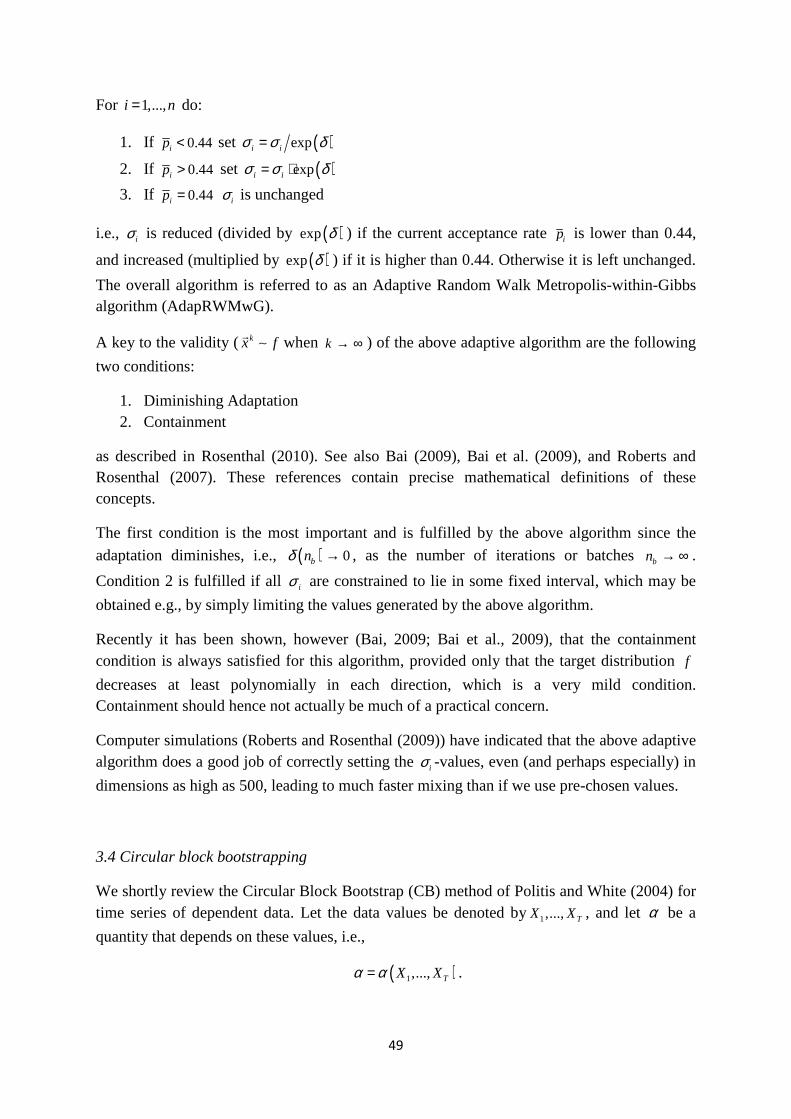
49

For 1,...,i n= do:

1. If 0.44ip < set ( )expi iσ σ δ=

2. If 0.44ip > set ( )expi iσ σ δ= ⋅

3. If 0.44ip = iσ is unchanged

i.e., iσ is reduced (divided by ( )exp δ ) if the current acceptance rate ip is lower than 0.44,

and increased (multiplied by ( )exp δ ) if it is higher than 0.44. Otherwise it is left unchanged.

The overall algorithm is referred to as an Adaptive Random Walk Metropolis-within-Gibbs algorithm (AdapRWMwG).

A key to the validity ( kx f∼ when k → ∞ ) of the above adaptive algorithm are the following

two conditions:

1. Diminishing Adaptation 2. Containment

as described in Rosenthal (2010). See also Bai (2009), Bai et al. (2009), and Roberts and Rosenthal (2007). These references contain precise mathematical definitions of these concepts.

The first condition is the most important and is fulfilled by the above algorithm since the

adaptation diminishes, i.e., ( ) 0bnδ → , as the number of iterations or batches bn → ∞ .

Condition 2 is fulfilled if all iσ are constrained to lie in some fixed interval, which may be

obtained e.g., by simply limiting the values generated by the above algorithm.

Recently it has been shown, however (Bai, 2009; Bai et al., 2009), that the containment condition is always satisfied for this algorithm, provided only that the target distribution f decreases at least polynomially in each direction, which is a very mild condition. Containment should hence not actually be much of a practical concern.

Computer simulations (Roberts and Rosenthal (2009)) have indicated that the above adaptive algorithm does a good job of correctly setting the iσ -values, even (and perhaps especially) in

dimensions as high as 500, leading to much faster mixing than if we use pre-chosen values.

3.4 Circular block bootstrapping

We shortly review the Circular Block Bootstrap (CB) method of Politis and White (2004) for time series of dependent data. Let the data values be denoted by 1,..., TX X , and let α be a

quantity that depends on these values, i.e.,

( )1,..., TX Xα α= .

50

We are interested in the uncertainty distribution of α , and thus we wish to define B new

bootstrapped time series 1 ,...,b bTX X with corresponding values bα , for 1,...,b B= , which can

be taken as an approximation to this distribution. Creating new bootstrapped time series by

simply drawing individual values btX with replacement from the original series is not

recommended, since this will generally destroy the dependence structure of the original time series, which may be of importance for the proper calculation of bootstrapped values of α .

The CB method is a nonparametric method which attempts to preserve the dependence structure of the original time series by sampling new values consecutively in blocks of fixed length. If we let N denote the number of blocks, L the fixed block length, and T NL= the total number of values in the time series, the CB algorithm is defined as follows:

For 1,...,b B= do:

1. Set 1k = .

2. Draw a new start index t uniformly from 1,...,T .

3. Define a new block of values 1 1,..., ,...,b bk k L t t LX X X X+ − + −= where the new values are

picked from the original series in a sequential and circular fashion, i.e., by replacing index t j+ by mod( , ) 1t j T+ + when t j T+ > .

4. Set k k L= + . 5. Repeat steps 2-4 N times to define a new bootstrapped time series 1 ,...,b b

TX X .

The algorithm thus uses potentially overlapping blocks in a circular fashion to define each new bootstrapped time series. Within each block, except when we wrap around, the original time series structure is preserved. It will, however, not be preserved at the joints between the different blocks, and thus the block length L is an important parameter.

According to Politis and White (2004) an estimated optimal block length for the circular block bootstrap can be calculated as follows:

1 3

21 3

,

ˆ2ˆˆopt CB

CB

GL T

D

=

where [ ]x denotes the nearest integer to the real number x , and where

( ) ( ) ( ) ( ) ( ) ( )2 24ˆ ˆ ˆ ˆˆ ˆ/ ; 0 ; 0 /3

M M

CBk M k M

G k M k R k D g g k M R kλ λ+ +

=− =−

= = =∑ ∑

with

( )ˆˆ ˆ 2 ; 0 for M m R k k m= ≈ >

and

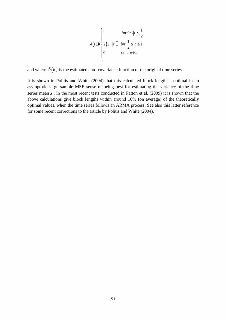
51

( ) ( )

11 for 0

21

2 1 for 12

0 otherwise

t

t t tλ

≤ ≤= − ≤ ≤

and where ( )R k is the estimated auto-covariance function of the original time series.

It is shown in Politis and White (2004) that this calculated block length is optimal in an asymptotic large sample MSE sense of being best for estimating the variance of the time

series meanX . In the most recent tests conducted in Patton et al. (2009) it is shown that the above calculations give block lengths within around 10% (on average) of the theoretically optimal values, when the time series follows an ARMA process. See also this latter reference for some recent corrections to the article by Politis and White (2004).

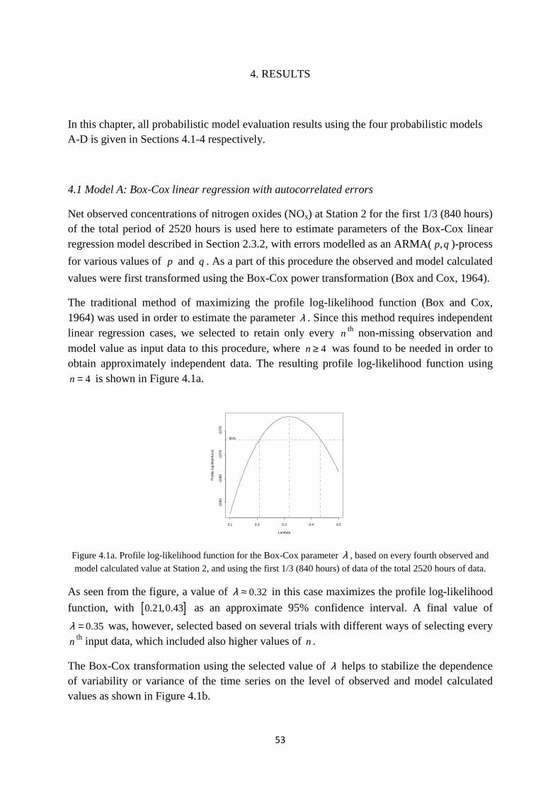
53

4. RESULTS

In this chapter, all probabilistic model evaluation results using the four probabilistic models A-D is given in Sections 4.1-4 respectively.

4.1 Model A: Box-Cox linear regression with autocorrelated errors

Net observed concentrations of nitrogen oxides (NOx) at Station 2 for the first 1/3 (840 hours) of the total period of 2520 hours is used here to estimate parameters of the Box-Cox linear regression model described in Section 2.3.2, with errors modelled as an ARMA(,p q )-process

for various values of p and q . As a part of this procedure the observed and model calculated

values were first transformed using the Box-Cox power transformation (Box and Cox, 1964).

The traditional method of maximizing the profile log-likelihood function (Box and Cox, 1964) was used in order to estimate the parameter λ . Since this method requires independent linear regression cases, we selected to retain only every n th non-missing observation and model value as input data to this procedure, where 4n ≥ was found to be needed in order to obtain approximately independent data. The resulting profile log-likelihood function using

4n = is shown in Figure 4.1a.

Figure 4.1a. Profile log-likelihood function for the Box-Cox parameter λ , based on every fourth observed and

model calculated value at Station 2, and using the first 1/3 (840 hours) of data of the total 2520 hours of data.

As seen from the figure, a value of 0.32λ ≈ in this case maximizes the profile log-likelihood

function, with [ ]0.21,0.43 as an approximate 95% confidence interval. A final value of

0.35λ = was, however, selected based on several trials with different ways of selecting every n th input data, which included also higher values of n .

The Box-Cox transformation using the selected value of λ helps to stabilize the dependence of variability or variance of the time series on the level of observed and model calculated values as shown in Figure 4.1b.

0.1 0.2 0.3 0.4 0.5

-108

2-1

080

-107

8-1

076

Lambda

Pro

file

log-

likel

ihoo

d

95%

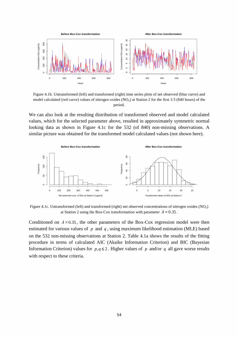
54

Figure 4.1b. Untransformed (left) and transformed (right) time series plots of net observed (blue curve) and model calculated (red curve) values of nitrogen oxides (NOx) at Station 2 for the first 1/3 (840 hours) of the

period.

We can also look at the resulting distribution of transformed observed and model calculated values, which for the selected parameter above, resulted in approximately symmetric normal looking data as shown in Figure 4.1c for the 532 (of 840) non-missing observations. A similar picture was obtained for the transformed model calculated values (not shown here).

Figure 4.1c. Untransformed (left) and transformed (right) net observed concentrations of nitrogen oxides (NOx) at Station 2 using the Box-Cox transformation with parameter 0.35λ = .

Conditioned on 0.35λ = , the other parameters of the Box-Cox regression model were then estimated for various values of p and q , using maximum likelihood estimation (MLE) based

on the 532 non-missing observations at Station 2. Table 4.1a shows the results of the fitting procedure in terms of calculated AIC (Akaike Information Criterion) and BIC (Bayesian Information Criterion) values for , 2p q≤ . Higher values of p and/or q all gave worse results

with respect to these criteria.

0 200 400 600 800

02

0040

060

080

0

Before Box-Cox transformation

Hours

Con

cent

ratio

n N

Ox

(ug/

m3)

0 200 400 600 800

-50

510

1520

2530

After Box-Cox transformation

Hours

Con

cent

ratio

n N

Ox

(ug/

m3)

Before Box-Cox transformation

Net observed conc. of NOx at Station 2 (ug/m3)

Fre

quen

cy

0 100 200 300 400 500 600

050

100

150

After Box-Cox transformation

Transformed values of NOx at Station 2

Fre

quen

cy

0 5 10 15 20 25

020

4060

80

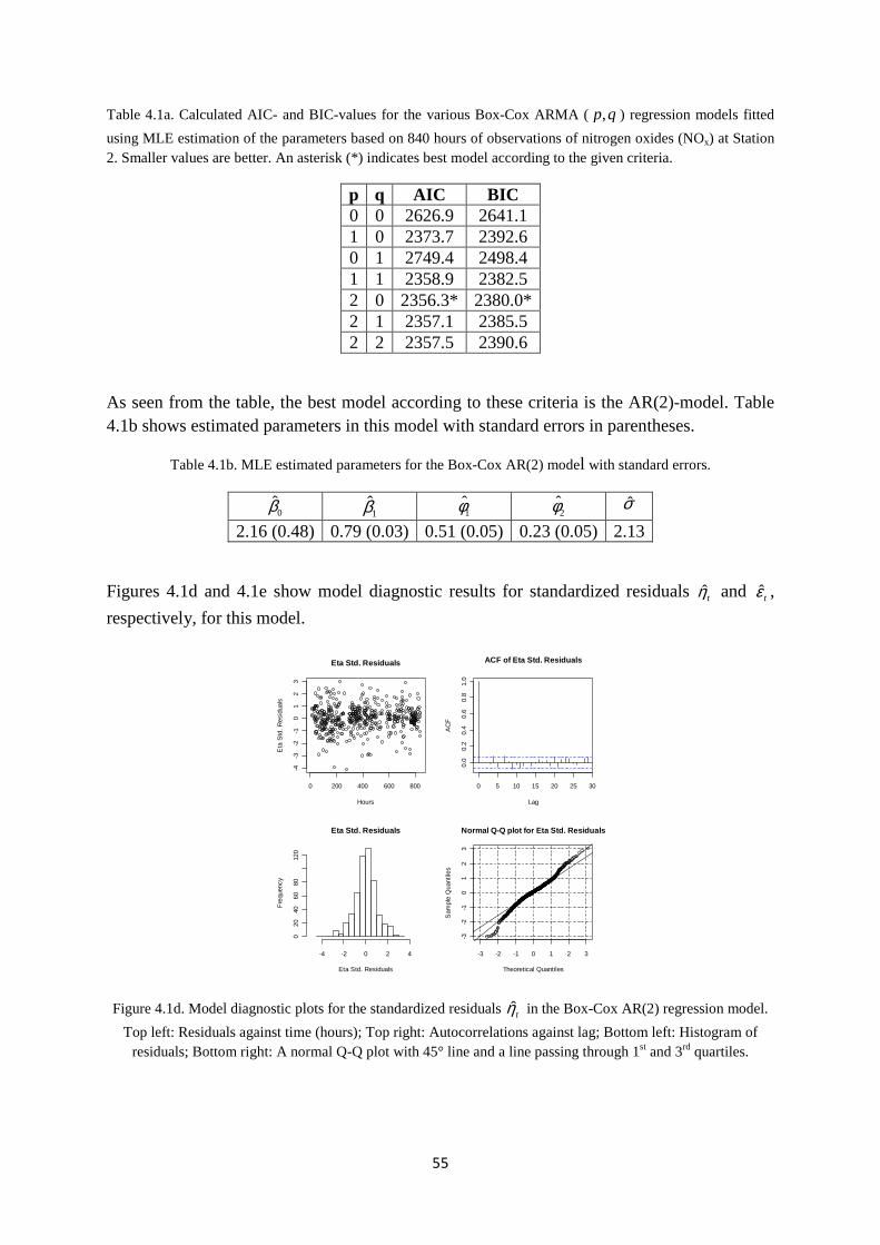
55

Table 4.1a. Calculated AIC- and BIC-values for the various Box-Cox ARMA ( ,p q ) regression models fitted

using MLE estimation of the parameters based on 840 hours of observations of nitrogen oxides (NOx) at Station 2. Smaller values are better. An asterisk (*) indicates best model according to the given criteria.

p q AIC BIC 0 0 2626.9 2641.1 1 0 2373.7 2392.6 0 1 2749.4 2498.4 1 1 2358.9 2382.5 2 0 2356.3* 2380.0* 2 1 2357.1 2385.5 2 2 2357.5 2390.6

As seen from the table, the best model according to these criteria is the AR(2)-model. Table 4.1b shows estimated parameters in this model with standard errors in parentheses.

Table 4.1b. MLE estimated parameters for the Box-Cox AR(2) model with standard errors.

0β 1β 1φ 2φ σ

2.16 (0.48) 0.79 (0.03) 0.51 (0.05) 0.23 (0.05) 2.13

Figures 4.1d and 4.1e show model diagnostic results for standardized residuals ˆtη and ˆ

tε ,

respectively, for this model.

Figure 4.1d. Model diagnostic plots for the standardized residuals tη in the Box-Cox AR(2) regression model.

Top left: Residuals against time (hours); Top right: Autocorrelations against lag; Bottom left: Histogram of residuals; Bottom right: A normal Q-Q plot with 45° line and a line passing through 1st and 3rd quartiles.

Eta Std. Residuals

Hours

Eta

Std

. R

esid

uals

0 200 400 600 800

-4-3

-2-1

01

23

0 5 10 15 20 25 30

0.0

0.2

0.4

0.6

0.8

1.0

Lag

AC

F

ACF of Eta Std. Residuals

Eta Std. Residuals

Eta Std. Residuals

Fre

quen

cy

-4 -2 0 2 4

020

4060

8012

0

-3 -2 -1 0 1 2 3

-3-2

-10

12

3

Normal Q-Q plot for Eta Std. Residuals

Theoretical Quantiles

Sam

ple

Qua

ntile

s

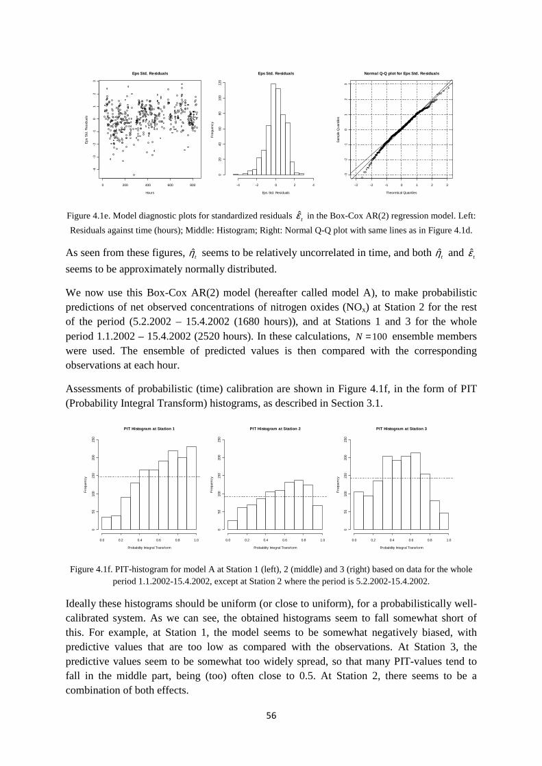
56

Figure 4.1e. Model diagnostic plots for standardized residuals tε in the Box-Cox AR(2) regression model. Left:

Residuals against time (hours); Middle: Histogram; Right: Normal Q-Q plot with same lines as in Figure 4.1d.

As seen from these figures, ˆtη seems to be relatively uncorrelated in time, and both ˆ

tη and ˆtε

seems to be approximately normally distributed.

We now use this Box-Cox AR(2) model (hereafter called model A), to make probabilistic predictions of net observed concentrations of nitrogen oxides (NOx) at Station 2 for the rest of the period (5.2.2002 – 15.4.2002 (1680 hours)), and at Stations 1 and 3 for the whole period 1.1.2002 – 15.4.2002 (2520 hours). In these calculations, 100N = ensemble members were used. The ensemble of predicted values is then compared with the corresponding observations at each hour.

Assessments of probabilistic (time) calibration are shown in Figure 4.1f, in the form of PIT (Probability Integral Transform) histograms, as described in Section 3.1.

Figure 4.1f. PIT-histogram for model A at Station 1 (left), 2 (middle) and 3 (right) based on data for the whole period 1.1.2002-15.4.2002, except at Station 2 where the period is 5.2.2002-15.4.2002.

Ideally these histograms should be uniform (or close to uniform), for a probabilistically well-calibrated system. As we can see, the obtained histograms seem to fall somewhat short of this. For example, at Station 1, the model seems to be somewhat negatively biased, with predictive values that are too low as compared with the observations. At Station 3, the predictive values seem to be somewhat too widely spread, so that many PIT-values tend to fall in the middle part, being (too) often close to 0.5. At Station 2, there seems to be a combination of both effects.

0 200 400 600 800

-4-3

-2-1

01

23

Eps Std. Residuals

Hours

Eps

Std

. Res

idua

ls

Eps Std. Residuals

Eps Std. Residuals

Fre

quen

cy

-4 -2 0 2 4

020

4060

8010

012

0

-3 -2 -1 0 1 2 3

-3-2

-10

12

3

Normal Q-Q plot for Eps Std. Residuals

Theoretical Quantiles

Sam

ple

Qua

ntile

s

PIT Histogram at Station 1

Probability Integral Transform

Fre

quen

cy

0.0 0.2 0.4 0.6 0.8 1.0

050

100

150

200

250



Fre

quen

cy

0.0 0.2 0.4 0.6 0.8 1.0

050

100

150

200

250



Fre

quen

cy

0.0 0.2 0.4 0.6 0.8 1.0

050

100

150

200

250

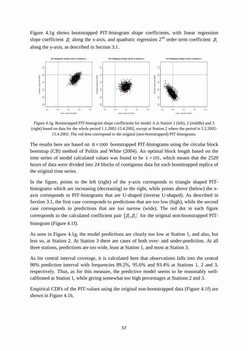
57

Figure 4.1g shows bootstrapped PIT-histogram shape coefficients, with linear regression slope coefficient 1β along the x-axis, and quadratic regression 2nd order term coefficient 2β

along the y-axis, as described in Section 3.1.

Figure 4.1g. Bootstrapped PIT-histogram shape coefficients for model A at Station 1 (left), 2 (middle) and 3 (right) based on data for the whole period 1.1.2002-15.4.2002, except at Station 2 where the period is 5.2.2002-

15.4.2002. The red dots correspond to the original (non-bootstrapped) PIT-histograms.

The results here are based on 1000B = bootstrapped PIT-histograms using the circular block bootstrap (CB) method of Politis and White (2004). An optimal block length based on the time series of model calculated values was found to be 105L = , which means that the 2520 hours of data were divided into 24 blocks of contiguous data for each bootstrapped replica of the original time series.

In the figure, points to the left (right) of the y-axis corresponds to triangle shaped PIT-histograms which are increasing (decreasing) to the right, while points above (below) the x-axis corresponds to PIT-histograms that are U-shaped (inverse U-shaped). As described in Section 3.1, the first case corresponds to predictions that are too low (high), while the second case corresponds to predictions that are too narrow (wide). The red dot in each figure

corresponds to the calculated coefficient pair ( )1 2,β β for the original non-bootstrapped PIT-

histogram (Figure 4.1f).

As seen in Figure 4.1g, the model predictions are clearly too low at Station 1, and also, but less so, at Station 2. At Station 3 there are cases of both over- and under-prediction. At all three stations, predictions are too wide, least at Station 1, and most at Station 3.

As for central interval coverage, it is calculated here that observations falls into the central 90% prediction interval with frequencies 89.2%, 95.6% and 93.4% at Stations 1, 2 and 3, respectively. Thus, as for this measure, the predictive model seems to be reasonably well-calibrated at Station 1, while giving somewhat too high percentages at Stations 2 and 3.

Empirical CDFs of the PIT-values using the original non-bootstrapped data (Figure 4.1f) are shown in Figure 4.1h.

-0.1 0.0 0.1 0.2 0.3

-0.8

-0.6

-0.4

-0.2

0.0

0.2

PIT Histogram Shape Coeff. at Station 1

Linear regression Beta1

Qua

drat

ic r

egre

ssio

n B

eta2

-0.1 0.0 0.1 0.2 0.3

-0.8

-0.6

-0.4

-0.2

0.0

0.2



Qua

drat

ic r

egre

ssio

n B

eta2

-0.1 0.0 0.1 0.2 0.3

-0.8

-0.6

-0.4

-0.2

0.0

0.2



Qua

drat

ic r

egre

ssio

n B

eta2

58

Figure 4.1h. Empirical CDFs of PIT-values for model A at Station 1 (left), 2 (middle) and 3 (right) based on data for the same periods as in Figure 4.1f. The dashed line indicates a 45° line of equal probabilities.

From this figure, we can clearly see that the model predictions are too low as compared to the observations at all cumulative probability levels p , except for 0.8p ≥ at Station 2 and

0.4p ≥ at Station 3, where the model predictions are too high. This is also reflected in the

marginal calibration evaluation using observed and predicted empirical CDFs as shown in Figure 4.1i.

Figure 4.1i. Marginal empirical CDFs of observed (solid line) and predicted (dashed line) concentration values for model A at Station 1 (left), 2 (middle) and 3 (right) based on data for the same periods as in Figure 4.1f.

As seen from the figure, the observed empirical CDF is always lower than the predicted, but the curves fit better as we move away from the road, i.e., from Station 1 to 3.

Sharpness diagrams (box plots) and associated data based on standard deviations and 90% central intervals for the predictive distributions at each of the three stations are shown in Figure 4.1j and Table 4.1c.

0.0 0.2 0.4 0.6 0.8 1.0

0.0

0.2

0.4

0.6

0.8

1.0

Empirical CDF of PIT values at Station 1

Probability

Pro

babi

lity

Inte

gral

Tra

nsfo

rm

0.0 0.2 0.4 0.6 0.8 1.0

0.0

0.2

0.4

0.6

0.8

1.0


Probability

Pro

babi

lity

Inte

gral

Tra

nsfo

rm

0.0 0.2 0.4 0.6 0.8 1.0

0.0

0.2

0.4

0.6

0.8

1.0


Probability

Pro

babi

lity

Inte

gral

Tra

nsfo

rm

0 200 400 600 800

0.0

0.2

0.4

0.6

0.8

1.0

Observed and Predicted Empirical CDFs at Station 1

Concentration NOx (ug/m3)

Pro

babi

lity

0 100 200 300 400 500 600

0.0

0.2

0.4

0.6

0.8

1.0



Pro

babi

lity

0 100 200 300 400 500 600

0.0

0.2

0.4

0.6

0.8

1.0



Pro

babi

lity

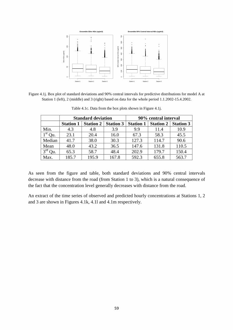
59

Figure 4.1j. Box plot of standard deviations and 90% central intervals for predictive distributions for model A at Station 1 (left), 2 (middle) and 3 (right) based on data for the whole period 1.1.2002-15.4.2002.

Table 4.1c. Data from the box plots shown in Figure 4.1j.

Standard deviation 90% central interval Station 1 Station 2 Station 3 Station 1 Station 2 Station 3 Min. 4.3 4.8 3.9 9.9 11.4 10.9 1st Qu. 23.1 20.4 16.0 67.3 58.3 45.5 Median 41.7 38.0 30.3 127.3 114.7 90.6 Mean 48.0 43.2 36.5 147.6 131.8 110.5 3rd Qu. 65.3 58.7 48.4 202.9 179.7 150.4 Max. 185.7 195.9 167.8 592.3 655.8 563.7

As seen from the figure and table, both standard deviations and 90% central intervals decrease with distance from the road (from Station 1 to 3), which is a natural consequence of the fact that the concentration level generally decreases with distance from the road.

An extract of the time series of observed and predicted hourly concentrations at Stations 1, 2 and 3 are shown in Figures 4.1k, 4.1l and 4.1m respectively.

Station 1 Station 2 Station 3

050

100

150

200

Ensemble SDev NOx (ug/m3)

SD

ev N

Ox

(ug/

m3)


010

020

030

040

050

060

070

0

Ensemble 90% Central Interval NOx (ug/m3)

90%

Cen

tral I

nter

val N

Ox

(ug/

m3)

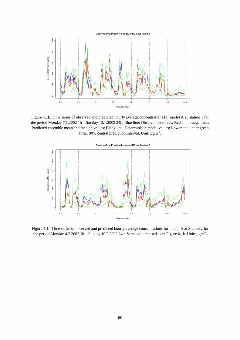
60

Figure 4.1k. Time series of observed and predicted hourly average concentrations for model A at Station 1 for the period Monday 7.1.2002 1h – Sunday 13.1.2002 24h. Blue line: Observation values; Red and orange lines: Predicted ensemble mean and median values; Black line: Deterministic model values; Lower and upper green

lines: 90% central prediction interval. Unit: µgm-3.

Figure 4.1l. Time series of observed and predicted hourly average concentrations for model A at Station 2 for the period Monday 4.2.2002 1h – Sunday 10.2.2002 24h. Same colours used as in Figure 4.1k. Unit: µgm-3.

Observed vs. Predicted conc. of NOx at Station 1

Days and hours

Con

cent

ratio

n N

Ox

(ug/

m3)

020

040

060

080

010

00

7.1 8.1 9.1 10.1 11.1 12.1 13.1 14.1


Days and hours

Con

cent

ratio

n N

Ox

(ug/

m3)

010

020

030

040

050

060

0

4.2 5.2 6.2 7.2 8.2 9.2 10.2 11.2

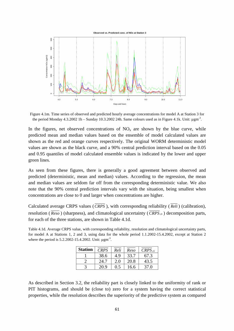
61

Figure 4.1m. Time series of observed and predicted hourly average concentrations for model A at Station 3 for the period Monday 4.3.2002 1h – Sunday 10.3.2002 24h. Same colours used as in Figure 4.1k. Unit: µgm-3.

In the figures, net observed concentrations of NOx are shown by the blue curve, while predicted mean and median values based on the ensemble of model calculated values are shown as the red and orange curves respectively. The original WORM deterministic model values are shown as the black curve, and a 90% central prediction interval based on the 0.05 and 0.95 quantiles of model calculated ensemble values is indicated by the lower and upper green lines.

As seen from these figures, there is generally a good agreement between observed and predicted (deterministic, mean and median) values. According to the regression, the mean and median values are seldom far off from the corresponding deterministic value. We also note that the 90% central prediction intervals vary with the situation, being smallest when concentrations are close to 0 and larger when concentrations are higher.

Calculated average CRPS values (CRPS), with corresponding reliability (Reli) (calibration),

resolution (Reso) (sharpness), and climatological uncertainty ( cliCRPS ) decomposition parts, for each of the three stations, are shown in Table 4.1d.

Table 4.1d. Average CRPS value, with corresponding reliability, resolution and climatological uncertainty parts, for model A at Stations 1, 2 and 3, using data for the whole period 1.1.2002-15.4.2002, except at Station 2 where the period is 5.2.2002-15.4.2002. Unit: µgm-3.

Station CRPS Reli Reso cliCRPS 1 38.6 4.9 33.7 67.3 2 24.7 2.0 20.8 43.5 3 20.9 0.5 16.6 37.0

As described in Section 3.2, the reliability part is closely linked to the uniformity of rank or PIT histograms, and should be (close to) zero for a system having the correct statistical properties, while the resolution describes the superiority of the predictive system as compared


Days and hours

Con

cent

ratio

n N

Ox

(ug/

m3)

010

020

030

040

050

060

0

4.3 5.3 6.3 7.3 8.3 9.3 10.3 11.3

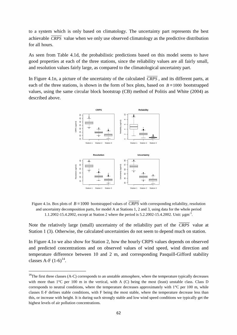
62

to a system which is only based on climatology. The uncertainty part represents the best

achievable CRPS value when we only use observed climatology as the predictive distribution for all hours.

As seen from Table 4.1d, the probabilistic predictions based on this model seems to have good properties at each of the three stations, since the reliability values are all fairly small, and resolution values fairly large, as compared to the climatological uncertainty part.

In Figure 4.1n, a picture of the uncertainty of the calculated CRPS, and its different parts, at each of the three stations, is shown in the form of box plots, based on 1000B = bootstrapped values, using the same circular block bootstrap (CB) method of Politis and White (2004) as described above.

Figure 4.1n. Box plots of 1000B = bootstrapped values of CRPSwith corresponding reliability, resolution

and uncertainty decomposition parts, for model A at Stations 1, 2 and 3, using data for the whole period 1.1.2002-15.4.2002, except at Station 2 where the period is 5.2.2002-15.4.2002. Unit: µgm-3.

Note the relatively large (small) uncertainty of the reliability part of the CRPS value at Station 1 (3). Otherwise, the calculated uncertainties do not seem to depend much on station.

In Figure 4.1o we also show for Station 2, how the hourly CRPS values depends on observed and predicted concentrations and on observed values of wind speed, wind direction and temperature difference between 10 and 2 m, and corresponding Pasquill-Gifford stability classes A-F (1-6)14.

14The first three classes (A-C) corresponds to an unstable atmosphere, where the temperature typically decreases with more than 1°C per 100 m in the vertical, with A (C) being the most (least) unstable class. Class D corresponds to neutral conditions, where the temperature decreases approximately with 1°C per 100 m, while classes E-F defines stable conditions, with F being the most stable, where the temperature decrease less than this, or increase with height. It is during such strongly stable and low wind speed conditions we typically get the highest levels of air pollution concentrations.


1520

2530

3540

4550

CRPS

CR

PS

(ug

/m3)


02

46

810

Reliability

Rel

iabi

lity

(ug/

m3)


1520

2530

3540

Resolution

Res

olut

ion

(ug/

m3)


3040

5060

7080

Uncertainty

Unc

erta

inty

(ug

/m3)

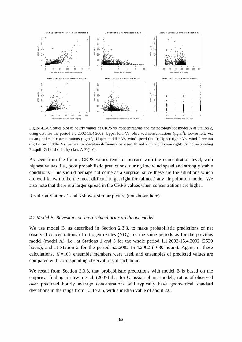
63

Figure 4.1o. Scatter plot of hourly values of CRPS vs. concentrations and meteorology for model A at Station 2, using data for the period 5.2.2002-15.4.2002. Upper left: Vs. observed concentrations (µgm-3); Lower left: Vs. mean predicted concentrations (µgm-3); Upper middle: Vs. wind speed (ms-1); Upper right: Vs. wind direction (°); Lower middle: Vs. vertical temperature difference between 10 and 2 m (°C); Lower right: Vs. corresponding Pasquill-Gifford stability class A-F (1-6).

As seen from the figure, CRPS values tend to increase with the concentration level, with highest values, i.e., poor probabilistic predictions, during low wind speed and strongly stable conditions. This should perhaps not come as a surprise, since these are the situations which are well-known to be the most difficult to get right for (almost) any air pollution model. We also note that there is a larger spread in the CRPS values when concentrations are higher.

Results at Stations 1 and 3 show a similar picture (not shown here).

4.2 Model B: Bayesian non-hierarchical prior predictive model

We use model B, as described in Section 2.3.3, to make probabilistic predictions of net observed concentrations of nitrogen oxides (NOx) for the same periods as for the previous model (model A), i.e., at Stations 1 and 3 for the whole period 1.1.2002-15.4.2002 (2520 hours), and at Station 2 for the period 5.2.2002-15.4.2002 (1680 hours). Again, in these calculations, 100N = ensemble members were used, and ensembles of predicted values are compared with corresponding observations at each hour.

We recall from Section 2.3.3, that probabilistic predictions with model B is based on the empirical findings in Irwin et al. (2007) that for Gaussian plume models, ratios of observed over predicted hourly average concentrations will typically have geometrical standard deviations in the range from 1.5 to 2.5, with a median value of about 2.0.

0 100 200 300 400 500 600

050

100

150

200

250

CRPS vs. Net Observed Conc. of NOx at Station 2

Net observed conc. of NOx at station 2 (ug/m3)

CR

PS

(ug

/m3)

0 2 4 6 8 10

050

100

150

200

250

CRPS at Station 2 vs. Wind Speed at 10 m

Wind speed at 10 m (m/s)

CR

PS

(ug

/m3)

0 50 100 150 200 250 300 350

050

100

150

200

250

CRPS at Station 2 vs. Wind Direction at 10 m

Wind direction at 10 m (deg)

CR

PS

(ug

/m3)

0 100 200 300 400 500 600

050

100

150

200

250

CRPS vs. Predicted Conc. of NOx at Station 2

Predicted conc. of NOx at station 2 (ug/m3)

CR

PS

(ug

/m3)

-1 0 1 2 3 4

050

100

150

200

250

CRPS at Station 2 vs. Temp. Diff. 10 - 2 m

Temperature dif ference betw een 10 and 2 m (deg C)

CR

PS

(ug

/m3)

1 2 3 4 5 6

050

100

150

200

250

CRPS at Station 2 vs. P-G Stability Class

Pasquill-Gifford stability class A=1,...,F=6

CR

PS

(ug

/m3)

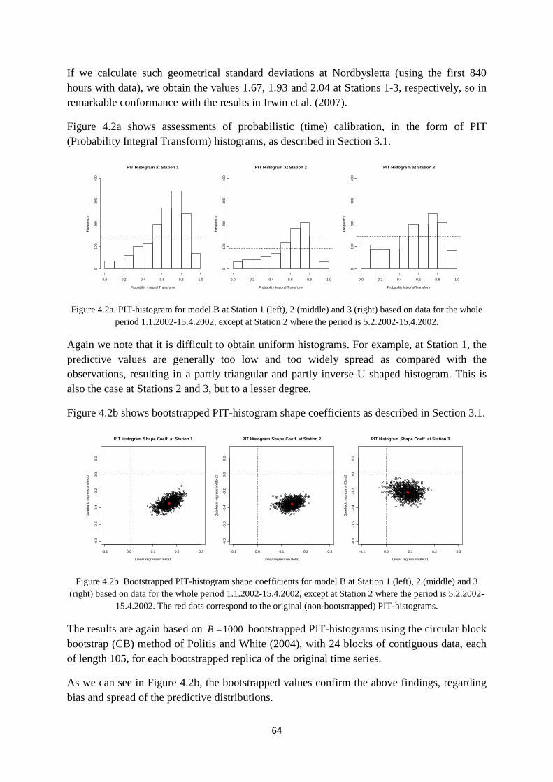
64

If we calculate such geometrical standard deviations at Nordbysletta (using the first 840 hours with data), we obtain the values 1.67, 1.93 and 2.04 at Stations 1-3, respectively, so in remarkable conformance with the results in Irwin et al. (2007).

Figure 4.2a shows assessments of probabilistic (time) calibration, in the form of PIT (Probability Integral Transform) histograms, as described in Section 3.1.

Figure 4.2a. PIT-histogram for model B at Station 1 (left), 2 (middle) and 3 (right) based on data for the whole period 1.1.2002-15.4.2002, except at Station 2 where the period is 5.2.2002-15.4.2002.

Again we note that it is difficult to obtain uniform histograms. For example, at Station 1, the predictive values are generally too low and too widely spread as compared with the observations, resulting in a partly triangular and partly inverse-U shaped histogram. This is also the case at Stations 2 and 3, but to a lesser degree.

Figure 4.2b shows bootstrapped PIT-histogram shape coefficients as described in Section 3.1.

Figure 4.2b. Bootstrapped PIT-histogram shape coefficients for model B at Station 1 (left), 2 (middle) and 3 (right) based on data for the whole period 1.1.2002-15.4.2002, except at Station 2 where the period is 5.2.2002-


The results are again based on 1000B = bootstrapped PIT-histograms using the circular block bootstrap (CB) method of Politis and White (2004), with 24 blocks of contiguous data, each of length 105, for each bootstrapped replica of the original time series.

As we can see in Figure 4.2b, the bootstrapped values confirm the above findings, regarding bias and spread of the predictive distributions.



Fre

quen

cy

0.0 0.2 0.4 0.6 0.8 1.0

010

020

030

040

0



Fre

quen

cy

0.0 0.2 0.4 0.6 0.8 1.0

010

020

030

040

0



Fre

quen

cy

0.0 0.2 0.4 0.6 0.8 1.0

010

020

030

040

0

-0.1 0.0 0.1 0.2 0.3

-0.8

-0.6

-0.4

-0.2

0.0

0.2



Qua

drat

ic r

egre

ssio

n B

eta2

-0.1 0.0 0.1 0.2 0.3

-0.8

-0.6

-0.4

-0.2

0.0

0.2



Qua

drat

ic r

egre

ssio

n B

eta2

-0.1 0.0 0.1 0.2 0.3

-0.8

-0.6

-0.4

-0.2

0.0

0.2



Qua

drat

ic r

egre

ssio

n B

eta2

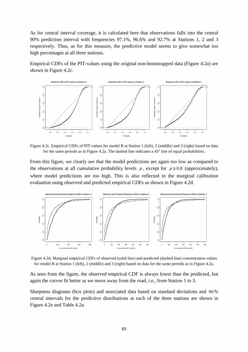
65

As for central interval coverage, it is calculated here that observations falls into the central 90% prediction interval with frequencies 97.1%, 96.6% and 92.7% at Stations 1, 2 and 3 respectively. Thus, as for this measure, the predictive model seems to give somewhat too high percentages at all three stations.

Empirical CDFs of the PIT-values using the original non-bootstrapped data (Figure 4.2a) are shown in Figure 4.2c.

Figure 4.2c. Empirical CDFs of PIT-values for model B at Station 1 (left), 2 (middle) and 3 (right) based on data for the same periods as in Figure 4.2a. The dashed line indicates a 45° line of equal probabilities.

From this figure, we clearly see that the model predictions are again too low as compared to the observations at all cumulative probability levels p , except for 0.8p ≥ (approximately),

where model predictions are too high. This is also reflected in the marginal calibration evaluation using observed and predicted empirical CDFs as shown in Figure 4.2d.

Figure 4.2d. Marginal empirical CDFs of observed (solid line) and predicted (dashed line) concentration values for model B at Station 1 (left), 2 (middle) and 3 (right) based on data for the same periods as in Figure 4.2a.

As seen from the figure, the observed empirical CDF is always lower than the predicted, but again the curves fit better as we move away from the road, i.e., from Station 1 to 3.

Sharpness diagrams (box plots) and associated data based on standard deviations and 90% central intervals for the predictive distributions at each of the three stations are shown in Figure 4.2e and Table 4.2a.

0.0 0.2 0.4 0.6 0.8 1.0

0.0

0.2

0.4

0.6

0.8

1.0


Probability

Pro

babi

lity

Inte

gral

Tra

nsfo

rm

0.0 0.2 0.4 0.6 0.8 1.0

0.0

0.2

0.4

0.6

0.8

1.0


Probability

Pro

babi

lity

Inte

gral

Tra

nsfo

rm

0.0 0.2 0.4 0.6 0.8 1.0

0.0

0.2

0.4

0.6

0.8

1.0


Probability

Pro

babi

lity

Inte

gral

Tra

nsfo

rm

0 200 400 600 800

0.0

0.2

0.4

0.6

0.8

1.0



Pro

babi

lity

0 100 200 300 400 500 600

0.0

0.2

0.4

0.6

0.8

1.0



Pro

babi

lity

0 100 200 300 400 500 600

0.0

0.2

0.4

0.6

0.8

1.0



Pro

babi

lity

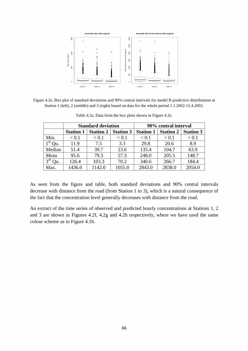
66

Figure 4.2e. Box plot of standard deviations and 90% central intervals for model B predictive distributions at Station 1 (left), 2 (middle) and 3 (right) based on data for the whole period 1.1.2002-15.4.2002.

Table 4.2a. Data from the box plots shown in Figure 4.2e.

Standard deviation 90% central interval Station 1 Station 2 Station 3 Station 1 Station 2 Station 3 Min. < 0.1 < 0.1 < 0.1 < 0.1 < 0.1 < 0.1 1st Qu. 11.9 7.5 3.3 29.8 20.6 8.9 Median 51.4 39.7 23.6 135.4 104.7 63.9 Mean 95.6 79.3 57.3 248.0 205.5 148.7 3rd Qu. 126.4 103.3 70.2 340.6 266.7 184.4 Max. 1436.0 1142.0 1055.0 2843.0 2838.0 2054.0


An extract of the time series of observed and predicted hourly concentrations at Stations 1, 2 and 3 are shown in Figures 4.2f, 4.2g and 4.2h respectively, where we have used the same colour scheme as in Figure 4.1h.


050

010

0015

00


SD

ev N

Ox

(ug/

m3)


050

010

0015

0020

0025

0030

00


90%

Cen

tral I

nter

val N

Ox

(ug/

m3)

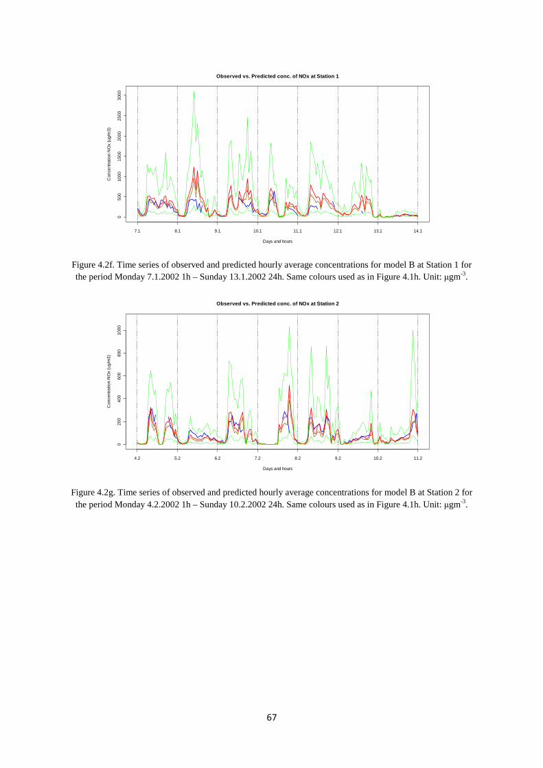
67

Figure 4.2f. Time series of observed and predicted hourly average concentrations for model B at Station 1 for the period Monday 7.1.2002 1h – Sunday 13.1.2002 24h. Same colours used as in Figure 4.1h. Unit: µgm-3.

Figure 4.2g. Time series of observed and predicted hourly average concentrations for model B at Station 2 for the period Monday 4.2.2002 1h – Sunday 10.2.2002 24h. Same colours used as in Figure 4.1h. Unit: µgm-3.


Days and hours

Con

cent

ratio

n N

Ox

(ug/

m3)

050

010

0015

0020

0025

0030

00

7.1 8.1 9.1 10.1 11.1 12.1 13.1 14.1


Days and hours

Con

cent

ratio

n N

Ox

(ug/

m3)

020

040

060

080

010

00

4.2 5.2 6.2 7.2 8.2 9.2 10.2 11.2

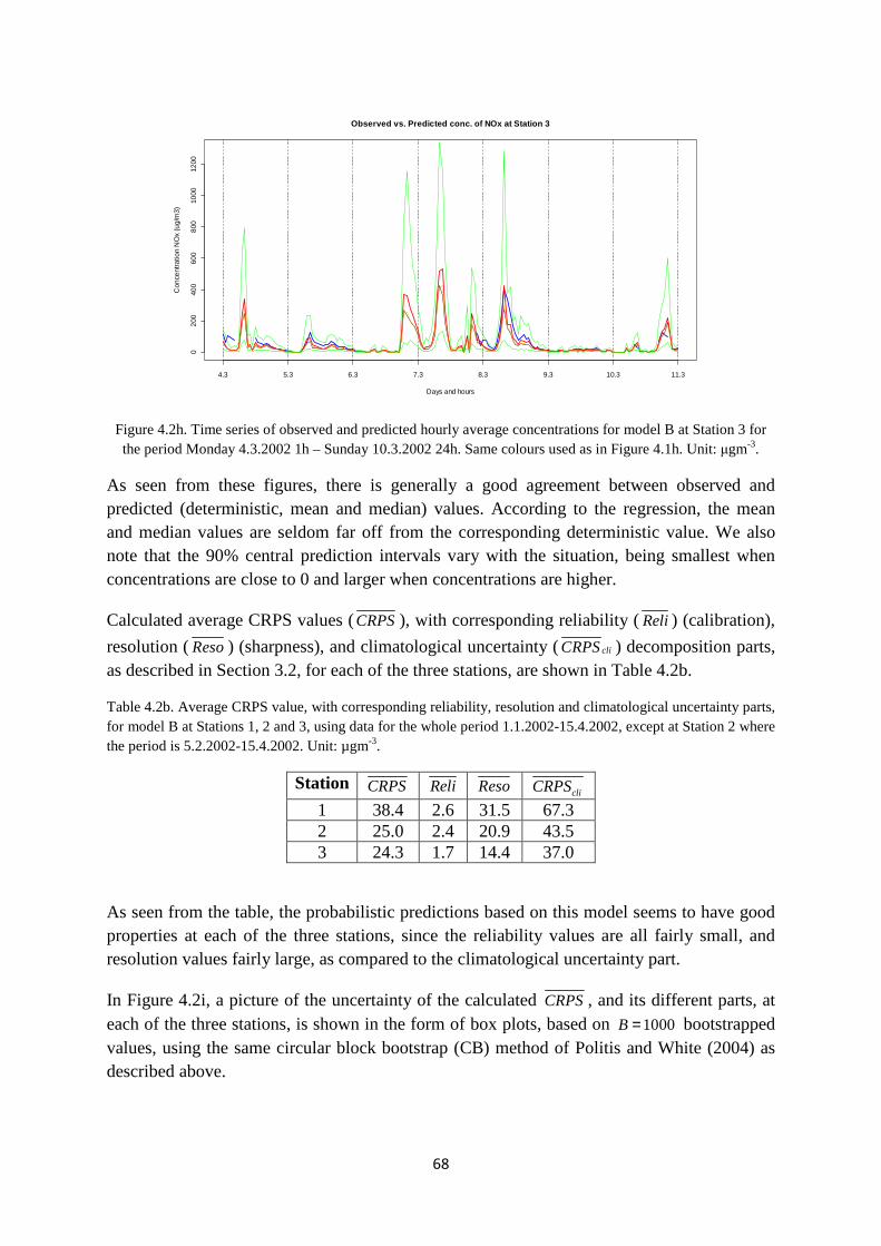
68

Figure 4.2h. Time series of observed and predicted hourly average concentrations for model B at Station 3 for the period Monday 4.3.2002 1h – Sunday 10.3.2002 24h. Same colours used as in Figure 4.1h. Unit: µgm-3.

As seen from these figures, there is generally a good agreement between observed and predicted (deterministic, mean and median) values. According to the regression, the mean and median values are seldom far off from the corresponding deterministic value. We also note that the 90% central prediction intervals vary with the situation, being smallest when concentrations are close to 0 and larger when concentrations are higher.


resolution (Reso) (sharpness), and climatological uncertainty ( cliCRPS ) decomposition parts, as described in Section 3.2, for each of the three stations, are shown in Table 4.2b.

Table 4.2b. Average CRPS value, with corresponding reliability, resolution and climatological uncertainty parts, for model B at Stations 1, 2 and 3, using data for the whole period 1.1.2002-15.4.2002, except at Station 2 where the period is 5.2.2002-15.4.2002. Unit: µgm-3.


As seen from the table, the probabilistic predictions based on this model seems to have good properties at each of the three stations, since the reliability values are all fairly small, and resolution values fairly large, as compared to the climatological uncertainty part.

In Figure 4.2i, a picture of the uncertainty of the calculated CRPS, and its different parts, at each of the three stations, is shown in the form of box plots, based on 1000B = bootstrapped values, using the same circular block bootstrap (CB) method of Politis and White (2004) as described above.


Days and hours

Con

cent

ratio

n N

Ox

(ug/

m3)

020

040

060

080

010

0012

00

4.3 5.3 6.3 7.3 8.3 9.3 10.3 11.3

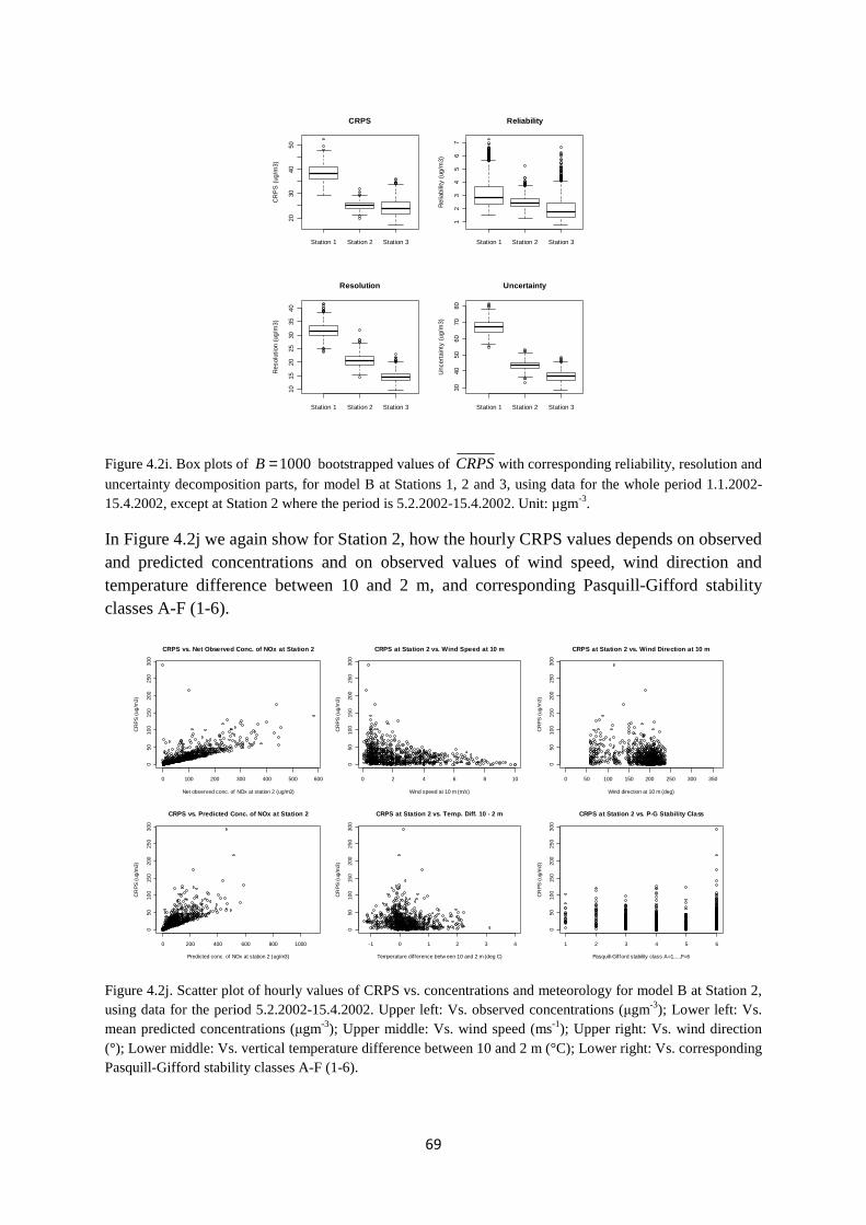
69

Figure 4.2i. Box plots of 1000B = bootstrapped values of CRPSwith corresponding reliability, resolution and

uncertainty decomposition parts, for model B at Stations 1, 2 and 3, using data for the whole period 1.1.2002-15.4.2002, except at Station 2 where the period is 5.2.2002-15.4.2002. Unit: µgm-3.

In Figure 4.2j we again show for Station 2, how the hourly CRPS values depends on observed and predicted concentrations and on observed values of wind speed, wind direction and temperature difference between 10 and 2 m, and corresponding Pasquill-Gifford stability classes A-F (1-6).

Figure 4.2j. Scatter plot of hourly values of CRPS vs. concentrations and meteorology for model B at Station 2, using data for the period 5.2.2002-15.4.2002. Upper left: Vs. observed concentrations (µgm-3); Lower left: Vs. mean predicted concentrations (µgm-3); Upper middle: Vs. wind speed (ms-1); Upper right: Vs. wind direction (°); Lower middle: Vs. vertical temperature difference between 10 and 2 m (°C); Lower right: Vs. corresponding Pasquill-Gifford stability classes A-F (1-6).


2030

4050

CRPS

CR

PS

(ug

/m3)


12

34

56

7

Reliability

Rel

iabi

lity

(ug/

m3)


1015

2025

3035

40Resolution

Res

olut

ion

(ug/

m3)


3040

5060

7080

Uncertainty

Unc

erta

inty

(ug

/m3)

0 100 200 300 400 500 600

050

100

150

200

250

300



CR

PS

(ug

/m3)

0 2 4 6 8 10

050

100

150

200

250

300



CR

PS

(ug

/m3)

0 50 100 150 200 250 300 350

050

100

150

200

250

300



CR

PS

(ug

/m3)

0 200 400 600 800 1000

050

100

150

200

250

300



CR

PS

(ug

/m3)

-1 0 1 2 3 4

050

100

150

200

250

300


Temperature difference betw een 10 and 2 m (deg C)

CR

PS

(ug

/m3)

1 2 3 4 5 6

050

100

150

200

250

300



CR

PS

(ug

/m3)

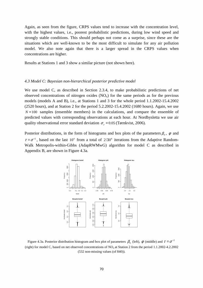
70

Again, as seen from the figure, CRPS values tend to increase with the concentration level, with the highest values, i.e., poorest probabilistic predictions, during low wind speed and strongly stable conditions. This should perhaps not come as a surprise, since these are the situations which are well-known to be the most difficult to simulate for any air pollution model. We also note again that there is a larger spread in the CRPS values when concentrations are higher.


4.3 Model C: Bayesian non-hierarchical posterior predictive model

We use model C, as described in Section 2.3.4, to make probabilistic predictions of net observed concentrations of nitrogen oxides (NOx) for the same periods as for the previous models (models A and B), i.e., at Stations 1 and 3 for the whole period 1.1.2002-15.4.2002 (2520 hours), and at Station 2 for the period 5.2.2002-15.4.2002 (1680 hours). Again, we use

100N = samples (ensemble members) in the calculations, and compare the ensemble of predicted values with corresponding observations at each hour. At Nordbysletta we use air quality observational error standard deviation 0.05yσ = (Tørnkvist, 2006).

Posterior distributions, in the form of histograms and box plots of the parameters0β , φ and 2τ σ −= , based on the last 410 from a total of 42 10⋅ iterations from the Adaptive Random-

Walk Metropolis-within-Gibbs (AdapRWMwG) algorithm for model C as described in Appendix B, are shown in Figure 4.3a.

Figure 4.3a. Posterior distribution histogram and box plot of parameters 0β (left), φ (middle) and 2τ σ −=

(right) for model C, based on net observed concentrations of NOx at Station 2 from the period 1.1.2002-4.2.2002 (532 non-missing values (of 840)).

Histogram beta0

beta0

Fre

quen

cy

-0.3 -0.1 0.0 0.1 0.2

050

010

0020

0030

00

Histogram phi

phi

Fre

quen

cy

0.45 0.55 0.65 0.75

050

010

0015

0020

00

Histogram tau

tau

Fre

quen

cy

3.0 3.5 4.0

050

010

0015

00

-0.2

-0.1

0.0

0.1

Boxplot beta0

Dis

trib

utio

n be

ta0

0.45

0.50

0.55

0.60

0.65

0.70

Boxplot phi

Dis

trib

utio

n ph

i

3.0

3.5

4.0

Boxplot tau

Dis

trib

utio

n ta

u

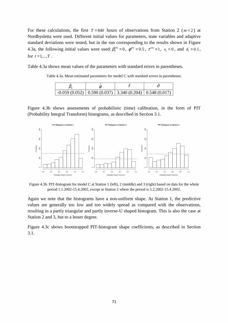
71

For these calculations, the first 840T = hours of observations from Station 2 ( 2m= ) at Nordbysletta were used. Different initial values for parameters, state variables and adaptive standard deviations were tested, but in the run corresponding to the results shown in Figure

4.3a, the following initial values were used:(0)0 0β = , (0) 0.5φ = , (0) 1τ = , 0tx = , and 0.1td = ,

for 1,...,t T= .

Table 4.3a shows mean values of the parameters with standard errors in parentheses.

Table 4.3a. Mean estimated parameters for model C with standard errors in parentheses.

0β φ τ σ

-0.059 (0.052) 0.590 (0.037) 3.340 (0.204) 0.548 (0.017)

Figure 4.3b shows assessments of probabilistic (time) calibration, in the form of PIT (Probability Integral Transform) histograms, as described in Section 3.1.

Figure 4.3b. PIT-histogram for model C at Station 1 (left), 2 (middle) and 3 (right) based on data for the whole period 1.1.2002-15.4.2002, except at Station 2 where the period is 5.2.2002-15.4.2002.

Again we note that the histograms have a non-uniform shape. At Station 1, the predictive values are generally too low and too widely spread as compared with the observations, resulting in a partly triangular and partly inverse-U shaped histogram. This is also the case at Station 2 and 3, but to a lesser degree.

Figure 4.3c shows bootstrapped PIT-histogram shape coefficients, as described in Section 3.1.



Fre

quen

cy

0.0 0.2 0.4 0.6 0.8 1.0

010

020

030

040

0



Fre

quen

cy

0.0 0.2 0.4 0.6 0.8 1.0

010

020

030

040

0



Fre

quen

cy

0.0 0.2 0.4 0.6 0.8 1.0

010

020

030

040

0

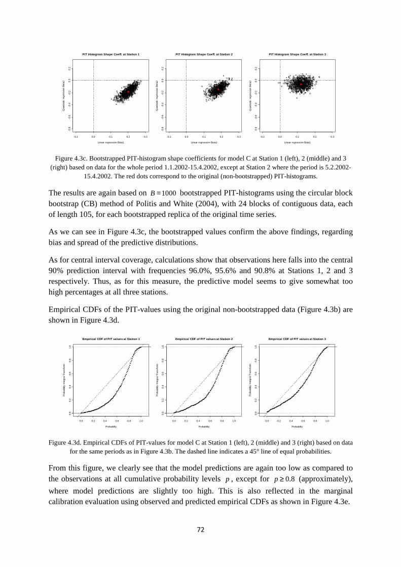
72

Figure 4.3c. Bootstrapped PIT-histogram shape coefficients for model C at Station 1 (left), 2 (middle) and 3 (right) based on data for the whole period 1.1.2002-15.4.2002, except at Station 2 where the period is 5.2.2002-



As we can see in Figure 4.3c, the bootstrapped values confirm the above findings, regarding bias and spread of the predictive distributions.

As for central interval coverage, calculations show that observations here falls into the central 90% prediction interval with frequencies 96.0%, 95.6% and 90.8% at Stations 1, 2 and 3 respectively. Thus, as for this measure, the predictive model seems to give somewhat too high percentages at all three stations.

Empirical CDFs of the PIT-values using the original non-bootstrapped data (Figure 4.3b) are shown in Figure 4.3d.

Figure 4.3d. Empirical CDFs of PIT-values for model C at Station 1 (left), 2 (middle) and 3 (right) based on data for the same periods as in Figure 4.3b. The dashed line indicates a 45° line of equal probabilities.


where model predictions are slightly too high. This is also reflected in the marginal calibration evaluation using observed and predicted empirical CDFs as shown in Figure 4.3e.

-0.1 0.0 0.1 0.2 0.3

-0.8

-0.6

-0.4

-0.2

0.0

0.2



Qua

drat

ic r

egre

ssio

n B

eta2

-0.1 0.0 0.1 0.2 0.3

-0.8

-0.6

-0.4

-0.2

0.0

0.2



Qua

drat

ic r

egre

ssio

n B

eta2

-0.1 0.0 0.1 0.2 0.3

-0.8

-0.6

-0.4

-0.2

0.0

0.2



Qua

drat

ic r

egre

ssio

n B

eta2

0.0 0.2 0.4 0.6 0.8 1.0

0.0

0.2

0.4

0.6

0.8

1.0


Probability

Pro

babi

lity

Inte

gral

Tra

nsfo

rm

0.0 0.2 0.4 0.6 0.8 1.0

0.0

0.2

0.4

0.6

0.8

1.0


Probability

Pro

babi

lity

Inte

gral

Tra

nsfo

rm

0.0 0.2 0.4 0.6 0.8 1.0

0.0

0.2

0.4

0.6

0.8

1.0


Probability

Pro

babi

lity

Inte

gral

Tra

nsfo

rm

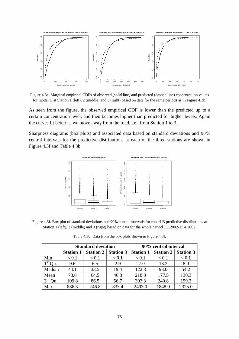
73

Figure 4.3e. Marginal empirical CDFs of observed (solid line) and predicted (dashed line) concentration values for model C at Station 1 (left), 2 (middle) and 3 (right) based on data for the same periods as in Figure 4.3b.

As seen from the figure, the observed empirical CDF is lower than the predicted up to a certain concentration level, and then becomes higher than predicted for higher levels. Again the curves fit better as we move away from the road, i.e., from Station 1 to 3.

Sharpness diagrams (box plots) and associated data based on standard deviations and 90% central intervals for the predictive distributions at each of the three stations are shown in Figure 4.3f and Table 4.3b.

Figure 4.3f. Box plot of standard deviations and 90% central intervals for model B predictive distributions at Station 1 (left), 2 (middle) and 3 (right) based on data for the whole period 1.1.2002-15.4.2002.

Table 4.3b. Data from the box plots shown in Figure 4.3f.


0 200 400 600 800

0.0

0.2

0.4

0.6

0.8

1.0



Pro

babi

lity

0 100 200 300 400 500 600

0.0

0.2

0.4

0.6

0.8

1.0



Pro

babi

lity

0 100 200 300 400 500 600

0.0

0.2

0.4

0.6

0.8

1.0



Pro

babi

lity


020

040

060

080

010

00


SD

ev N

Ox

(ug/

m3)


050

010

0015

0020

0025

00


90%

Cen

tral I

nter

val N

Ox

(ug/

m3)

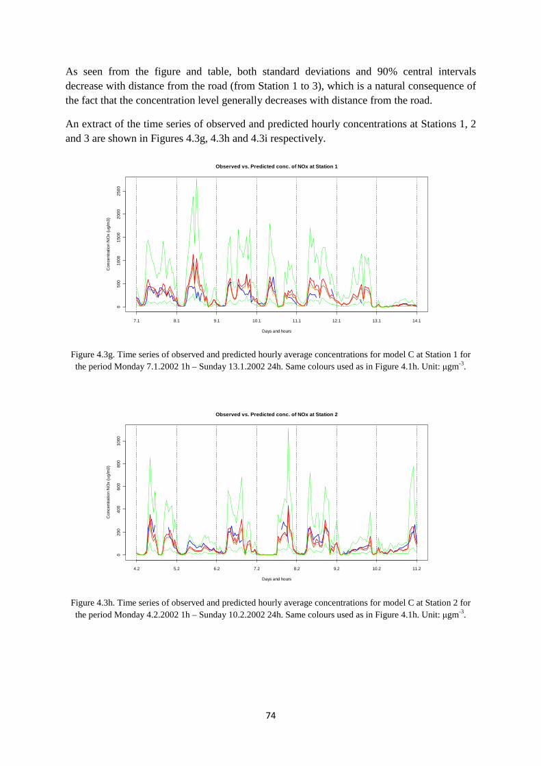
74


An extract of the time series of observed and predicted hourly concentrations at Stations 1, 2 and 3 are shown in Figures 4.3g, 4.3h and 4.3i respectively.

Figure 4.3g. Time series of observed and predicted hourly average concentrations for model C at Station 1 for the period Monday 7.1.2002 1h – Sunday 13.1.2002 24h. Same colours used as in Figure 4.1h. Unit: µgm-3.

Figure 4.3h. Time series of observed and predicted hourly average concentrations for model C at Station 2 for the period Monday 4.2.2002 1h – Sunday 10.2.2002 24h. Same colours used as in Figure 4.1h. Unit: µgm-3.


Days and hours

Con

cent

ratio

n N

Ox

(ug/

m3)

050

010

0015

0020

0025

00

7.1 8.1 9.1 10.1 11.1 12.1 13.1 14.1


Days and hours

Con

cent

ratio

n N

Ox

(ug/

m3)

020

040

060

080

010

00

4.2 5.2 6.2 7.2 8.2 9.2 10.2 11.2

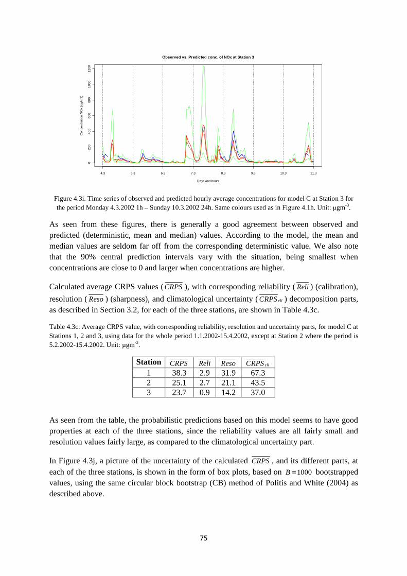
75

Figure 4.3i. Time series of observed and predicted hourly average concentrations for model C at Station 3 for the period Monday 4.3.2002 1h – Sunday 10.3.2002 24h. Same colours used as in Figure 4.1h. Unit: µgm-3.

As seen from these figures, there is generally a good agreement between observed and predicted (deterministic, mean and median) values. According to the model, the mean and median values are seldom far off from the corresponding deterministic value. We also note that the 90% central prediction intervals vary with the situation, being smallest when concentrations are close to 0 and larger when concentrations are higher.


resolution (Reso) (sharpness), and climatological uncertainty ( cliCRPS ) decomposition parts, as described in Section 3.2, for each of the three stations, are shown in Table 4.3c.

Table 4.3c. Average CRPS value, with corresponding reliability, resolution and uncertainty parts, for model C at Stations 1, 2 and 3, using data for the whole period 1.1.2002-15.4.2002, except at Station 2 where the period is 5.2.2002-15.4.2002. Unit: µgm-3.


As seen from the table, the probabilistic predictions based on this model seems to have good properties at each of the three stations, since the reliability values are all fairly small and resolution values fairly large, as compared to the climatological uncertainty part.

In Figure 4.3j, a picture of the uncertainty of the calculated CRPS, and its different parts, at each of the three stations, is shown in the form of box plots, based on 1000B = bootstrapped values, using the same circular block bootstrap (CB) method of Politis and White (2004) as described above.


Days and hours

Con

cent

ratio

n N

Ox

(ug/

m3)

020

040

060

080

010

0012

00

4.3 5.3 6.3 7.3 8.3 9.3 10.3 11.3

76

Figure 4.3j. Box plots of 1000B = bootstrapped values of CRPSwith corresponding reliability, resolution and

uncertainty decomposition parts, for model C at Stations 1, 2 and 3, using data for the whole period 1.1.2002-15.4.2002, except at Station 2 where the period is 5.2.2002-15.4.2002. Unit: µgm-3.

In Figure 4.3k we again show for Station 2, how the hourly CRPS values depends on observed and predicted concentrations and on observed values of wind speed, wind direction and temperature difference between 10 and 2 m, and corresponding Pasquill-Gifford stability classes A-F (1-6).

Figure 4.3k. Scatter plot of hourly values of CRPS vs. concentrations and meteorology for model C at Station 2, using data for the period 5.2.2002-15.4.2002. Upper left: Vs. observed concentrations (µgm-3); Lower left: Vs. mean predicted concentrations (µgm-3); Upper middle: Vs. wind speed (ms-1); Upper right: Vs. wind direction (°); Lower middle: Vs. vertical temperature difference between 10 and 2 m (°C); Lower right: Vs. corresponding Pasquill-Gifford stability classes A-F (1-6).


2025

3035

4045

CRPS

CR

PS

(ug

/m3)


24

68

Reliability

Rel

iabi

lity

(ug/

m3)


1015

2025

3035

40Resolution

Res

olut

ion

(ug/

m3)


3040

5060

7080

Uncertainty

Unc

erta

inty

(ug

/m3)

0 100 200 300 400 500 600

050

100

150

200

250



CR

PS

(ug

/m3)

0 2 4 6 8 10

050

100

150

200

250



CR

PS

(ug

/m3)

0 50 100 150 200 250 300 350

050

100

150

200

250



CR

PS

(ug

/m3)

0 200 400 600 800

050

100

150

200

250



CR

PS

(ug

/m3)

-1 0 1 2 3 4

050

100

150

200

250


Temperature dif ference betw een 10 and 2 m (deg C)

CR

PS

(ug

/m3)

1 2 3 4 5 6

050

100

150

200

250



CR

PS

(ug

/m3)

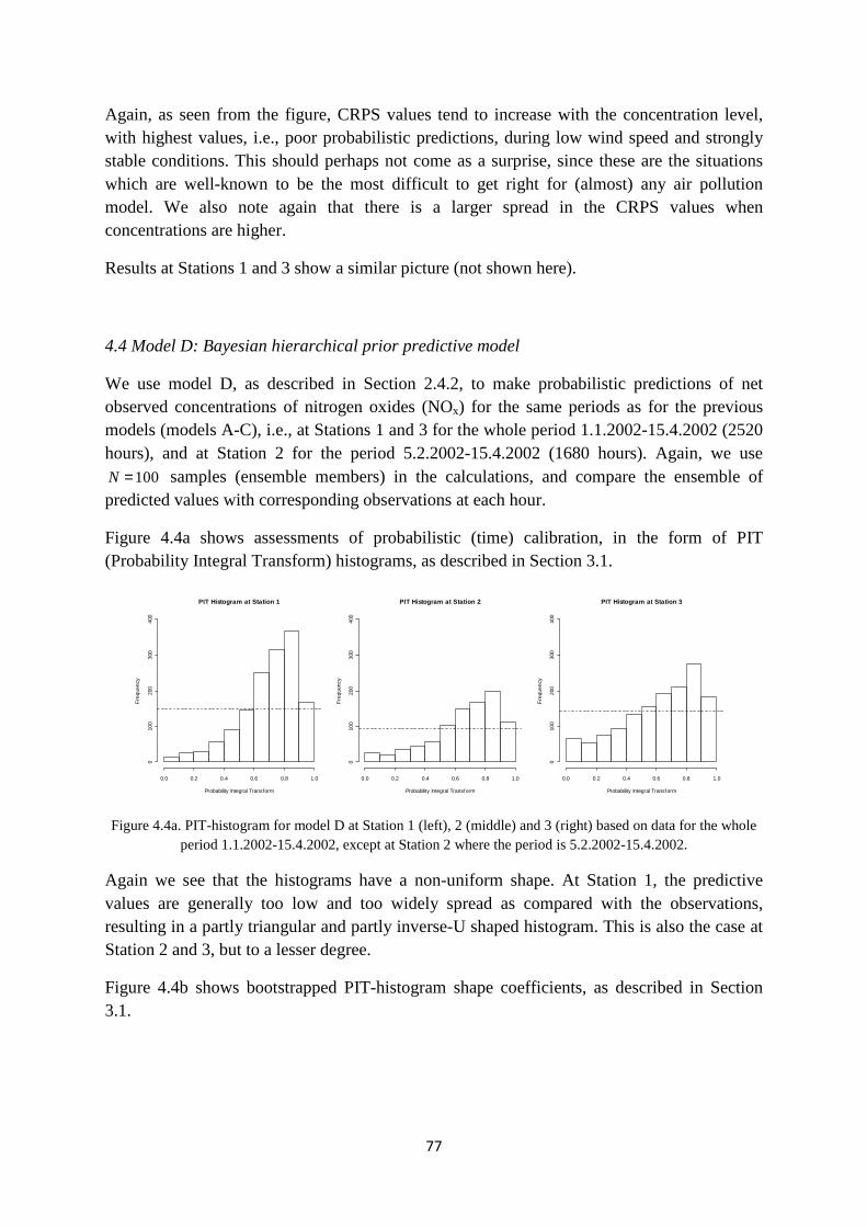
77

Again, as seen from the figure, CRPS values tend to increase with the concentration level, with highest values, i.e., poor probabilistic predictions, during low wind speed and strongly stable conditions. This should perhaps not come as a surprise, since these are the situations which are well-known to be the most difficult to get right for (almost) any air pollution model. We also note again that there is a larger spread in the CRPS values when concentrations are higher.


4.4 Model D: Bayesian hierarchical prior predictive model

We use model D, as described in Section 2.4.2, to make probabilistic predictions of net observed concentrations of nitrogen oxides (NOx) for the same periods as for the previous models (models A-C), i.e., at Stations 1 and 3 for the whole period 1.1.2002-15.4.2002 (2520 hours), and at Station 2 for the period 5.2.2002-15.4.2002 (1680 hours). Again, we use

100N = samples (ensemble members) in the calculations, and compare the ensemble of predicted values with corresponding observations at each hour.

Figure 4.4a shows assessments of probabilistic (time) calibration, in the form of PIT (Probability Integral Transform) histograms, as described in Section 3.1.

Figure 4.4a. PIT-histogram for model D at Station 1 (left), 2 (middle) and 3 (right) based on data for the whole period 1.1.2002-15.4.2002, except at Station 2 where the period is 5.2.2002-15.4.2002.

Again we see that the histograms have a non-uniform shape. At Station 1, the predictive values are generally too low and too widely spread as compared with the observations, resulting in a partly triangular and partly inverse-U shaped histogram. This is also the case at Station 2 and 3, but to a lesser degree.

Figure 4.4b shows bootstrapped PIT-histogram shape coefficients, as described in Section 3.1.



Fre

quen

cy

0.0 0.2 0.4 0.6 0.8 1.0

010

020

030

040

0



Fre

quen

cy

0.0 0.2 0.4 0.6 0.8 1.0

010

020

030

040

0



Fre

quen

cy

0.0 0.2 0.4 0.6 0.8 1.0

010

020

030

040

0

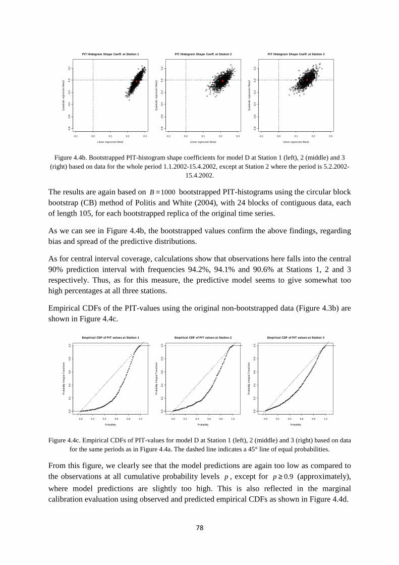
78

Figure 4.4b. Bootstrapped PIT-histogram shape coefficients for model D at Station 1 (left), 2 (middle) and 3 (right) based on data for the whole period 1.1.2002-15.4.2002, except at Station 2 where the period is 5.2.2002-

15.4.2002.


As we can see in Figure 4.4b, the bootstrapped values confirm the above findings, regarding bias and spread of the predictive distributions.

As for central interval coverage, calculations show that observations here falls into the central 90% prediction interval with frequencies 94.2%, 94.1% and 90.6% at Stations 1, 2 and 3 respectively. Thus, as for this measure, the predictive model seems to give somewhat too high percentages at all three stations.

Empirical CDFs of the PIT-values using the original non-bootstrapped data (Figure 4.3b) are shown in Figure 4.4c.

Figure 4.4c. Empirical CDFs of PIT-values for model D at Station 1 (left), 2 (middle) and 3 (right) based on data for the same periods as in Figure 4.4a. The dashed line indicates a 45° line of equal probabilities.


where model predictions are slightly too high. This is also reflected in the marginal calibration evaluation using observed and predicted empirical CDFs as shown in Figure 4.4d.

-0.1 0.0 0.1 0.2 0.3

-0.8

-0.6

-0.4

-0.2

0.0

0.2



Qua

drat

ic r

egre

ssio

n B

eta2

-0.1 0.0 0.1 0.2 0.3

-0.8

-0.6

-0.4

-0.2

0.0

0.2



Qua

drat

ic r

egre

ssio

n B

eta2

-0.1 0.0 0.1 0.2 0.3

-0.8

-0.6

-0.4

-0.2

0.0

0.2



Qua

drat

ic r

egre

ssio

n B

eta2

0.0 0.2 0.4 0.6 0.8 1.0

0.0

0.2

0.4

0.6

0.8

1.0


Probability

Pro

babi

lity

Inte

gral

Tra

nsfo

rm

0.0 0.2 0.4 0.6 0.8 1.0

0.0

0.2

0.4

0.6

0.8

1.0


Probability

Pro

babi

lity

Inte

gral

Tra

nsfo

rm

0.0 0.2 0.4 0.6 0.8 1.0

0.0

0.2

0.4

0.6

0.8

1.0


Probability

Pro

babi

lity

Inte

gral

Tra

nsfo

rm

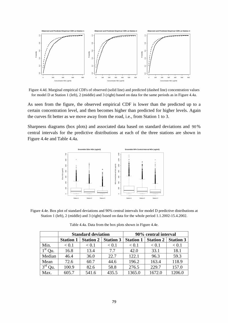
79

Figure 4.4d. Marginal empirical CDFs of observed (solid line) and predicted (dashed line) concentration values for model D at Station 1 (left), 2 (middle) and 3 (right) based on data for the same periods as in Figure 4.4a.

As seen from the figure, the observed empirical CDF is lower than the predicted up to a certain concentration level, and then becomes higher than predicted for higher levels. Again the curves fit better as we move away from the road, i.e., from Station 1 to 3.

Sharpness diagrams (box plots) and associated data based on standard deviations and 90% central intervals for the predictive distributions at each of the three stations are shown in Figure 4.4e and Table 4.4a.

Figure 4.4e. Box plot of standard deviations and 90% central intervals for model D predictive distributions at Station 1 (left), 2 (middle) and 3 (right) based on data for the whole period 1.1.2002-15.4.2002.

Table 4.4a. Data from the box plots shown in Figure 4.4e.


0 200 400 600 800

0.0

0.2

0.4

0.6

0.8

1.0



Pro

babi

lity

0 100 200 300 400 500 600

0.0

0.2

0.4

0.6

0.8

1.0



Pro

babi

lity

0 100 200 300 400 500 600

0.0

0.2

0.4

0.6

0.8

1.0



Pro

babi

lity


010

020

030

040

050

060

070

0


SD

ev N

Ox

(ug/

m3)


020

040

060

080

010

0012

0014

00


90%

Cen

tral I

nter

val N

Ox

(ug/

m3)

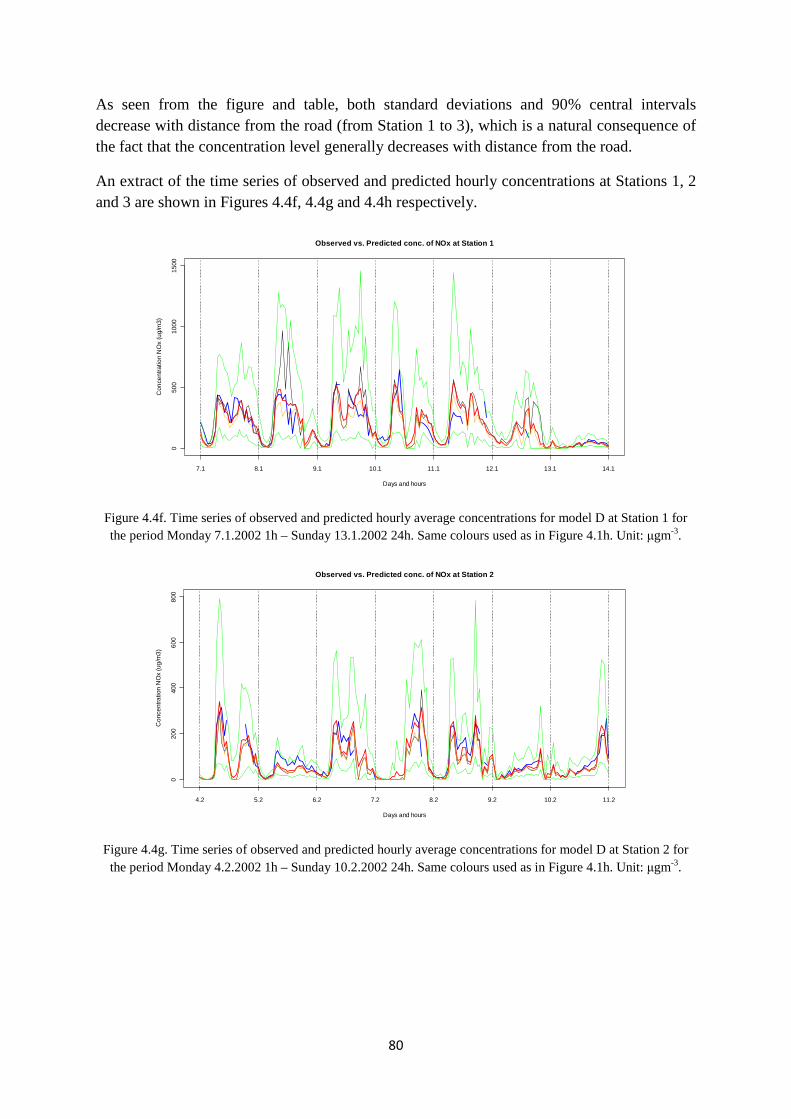
80


An extract of the time series of observed and predicted hourly concentrations at Stations 1, 2 and 3 are shown in Figures 4.4f, 4.4g and 4.4h respectively.

Figure 4.4f. Time series of observed and predicted hourly average concentrations for model D at Station 1 for the period Monday 7.1.2002 1h – Sunday 13.1.2002 24h. Same colours used as in Figure 4.1h. Unit: µgm-3.

Figure 4.4g. Time series of observed and predicted hourly average concentrations for model D at Station 2 for the period Monday 4.2.2002 1h – Sunday 10.2.2002 24h. Same colours used as in Figure 4.1h. Unit: µgm-3.


Days and hours

Con

cent

ratio

n N

Ox

(ug/

m3)

050

010

0015

00

7.1 8.1 9.1 10.1 11.1 12.1 13.1 14.1


Days and hours

Con

cent

ratio

n N

Ox

(ug/

m3)

020

040

060

080

0

4.2 5.2 6.2 7.2 8.2 9.2 10.2 11.2

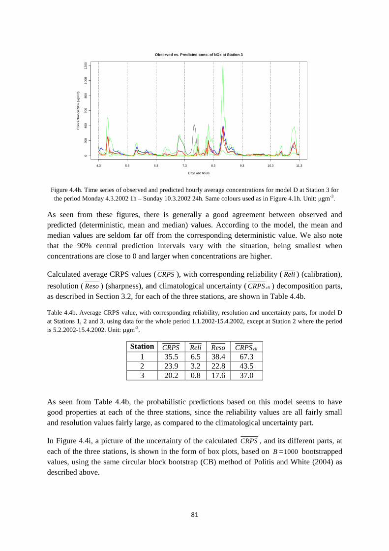
81

Figure 4.4h. Time series of observed and predicted hourly average concentrations for model D at Station 3 for the period Monday 4.3.2002 1h – Sunday 10.3.2002 24h. Same colours used as in Figure 4.1h. Unit: µgm-3.

As seen from these figures, there is generally a good agreement between observed and predicted (deterministic, mean and median) values. According to the model, the mean and median values are seldom far off from the corresponding deterministic value. We also note that the 90% central prediction intervals vary with the situation, being smallest when concentrations are close to 0 and larger when concentrations are higher.


resolution (Reso) (sharpness), and climatological uncertainty ( cliCRPS ) decomposition parts, as described in Section 3.2, for each of the three stations, are shown in Table 4.4b.

Table 4.4b. Average CRPS value, with corresponding reliability, resolution and uncertainty parts, for model D at Stations 1, 2 and 3, using data for the whole period 1.1.2002-15.4.2002, except at Station 2 where the period is 5.2.2002-15.4.2002. Unit: µgm-3.


As seen from Table 4.4b, the probabilistic predictions based on this model seems to have good properties at each of the three stations, since the reliability values are all fairly small and resolution values fairly large, as compared to the climatological uncertainty part.

In Figure 4.4i, a picture of the uncertainty of the calculated CRPS, and its different parts, at each of the three stations, is shown in the form of box plots, based on 1000B = bootstrapped values, using the same circular block bootstrap (CB) method of Politis and White (2004) as described above.


Days and hours

Con

cent

ratio

n N

Ox

(ug/

m3)

020

040

060

080

010

0012

00

4.3 5.3 6.3 7.3 8.3 9.3 10.3 11.3

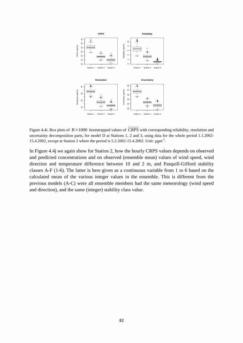
82

Figure 4.4i. Box plots of 1000B = bootstrapped values of CRPSwith corresponding reliability, resolution and

uncertainty decomposition parts, for model D at Stations 1, 2 and 3, using data for the whole period 1.1.2002-15.4.2002, except at Station 2 where the period is 5.2.2002-15.4.2002. Unit: µgm-3.

In Figure 4.4j we again show for Station 2, how the hourly CRPS values depends on observed and predicted concentrations and on observed (ensemble mean) values of wind speed, wind direction and temperature difference between 10 and 2 m, and Pasquill-Gifford stability classes A-F (1-6). The latter is here given as a continuous variable from 1 to 6 based on the calculated mean of the various integer values in the ensemble. This is different from the previous models (A-C) were all ensemble members had the same meteorology (wind speed and direction), and the same (integer) stability class value.


1520

2530

3540

45

CRPS

CR

PS

(ug

/m3)


02

46

810

Reliability

Rel

iabi

lity

(ug/

m3)


1525

3545

Resolution

Res

olut

ion

(ug/

m3)


3040

5060

7080

Uncertainty

Unc

erta

inty

(ug

/m3)

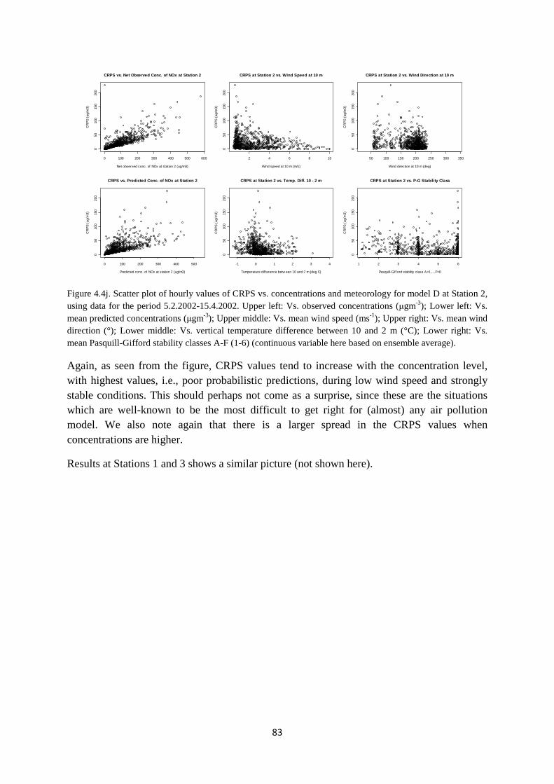
83

Figure 4.4j. Scatter plot of hourly values of CRPS vs. concentrations and meteorology for model D at Station 2, using data for the period 5.2.2002-15.4.2002. Upper left: Vs. observed concentrations (µgm-3); Lower left: Vs. mean predicted concentrations (µgm-3); Upper middle: Vs. mean wind speed (ms-1); Upper right: Vs. mean wind direction (°); Lower middle: Vs. vertical temperature difference between 10 and 2 m (°C); Lower right: Vs. mean Pasquill-Gifford stability classes A-F (1-6) (continuous variable here based on ensemble average).

Again, as seen from the figure, CRPS values tend to increase with the concentration level, with highest values, i.e., poor probabilistic predictions, during low wind speed and strongly stable conditions. This should perhaps not come as a surprise, since these are the situations which are well-known to be the most difficult to get right for (almost) any air pollution model. We also note again that there is a larger spread in the CRPS values when concentrations are higher.

Results at Stations 1 and 3 shows a similar picture (not shown here).

0 100 200 300 400 500 600

050

100

150

200



CR

PS

(ug

/m3)

2 4 6 8 10

050

100

150

200



CR

PS

(ug

/m3)

50 100 150 200 250 300 350

050

100

150

200



CR

PS

(ug

/m3)

0 100 200 300 400 500

050

100

150

200



CR

PS

(ug

/m3)

-1 0 1 2 3 4

050

100

150

200


Temperature difference betw een 10 and 2 m (deg C)

CR

PS

(ug

/m3)

1 2 3 4 5 6

050

100

150

200


Pasquill-Gif ford stability class A=1,...,F=6

CR

PS

(ug

/m3)

85

5. DISCUSSION AND CONCLUSIONS

5.1 Discussion

Four probabilistic models for prediction of NOx concentrations with uncertainty from road traffic are presented. All models use the deterministic WORM model for defining the mean spatial and temporal characteristics of concentrations from the given roads or road-segments. In connection to this, four stochastic models were developed and tested using data from Nordbysletta in 2002. The following table summarizes some of the main characteristics of these models.

Table 5.1a. Main characteristics of proposed stochastic models.

Model Type Treating WORM as a black box?

Transform of conc. Handling of parameters

A Classical Yes Box-Cox MLE based on local NOx

observations

B Bayesian Yes Logarithmic Prior based on international

monitoring campaigns

C Bayesian Yes Logarithmic Posterior based on local NOx

observations

D Bayesian No Logarithmic Prior based on NILU expert

elicitation

We will first shortly discuss results of the probabilistic model evaluations performed for these models as given in Chapter 4, before we give some main conclusions in the next section.

All models generate somewhat too low predicted concentrations as compared with observations, especially at Stations 1 and 2, resulting in triangle shaped PIT-histograms. The main reason for this is that the WORM model predicts somewhat too low concentrations as compared with observations at Nordbysletta. The stochastic models have thus, not managed to fully correct for this bias in the dispersion model.

Models A and B (and partly also C) produces somewhat too wide predictions compared with observations, resulting in inverse-U shaped PIT-histograms. This is especially the case for model A at Station 3, and for model B at Station 1.

As for the 90% predicted central interval coverage, all models give higher values than 90% at all stations, except for model A at Station 1 with 89.2%, the worst case being model B at Station 1 with a coverage value of 97.1%.

Observed and predicted marginal CDFs fits best at Station 3 and worst at Station 1 for all models. Otherwise, it is difficult to rank the models regarding this.

Comparing sharpness using mean and maximum values of standard deviations and 90% central prediction intervals, we find that model A is clearly best, followed by model D, and with models C and B being worse than these two. This is also evident when we look at time

86

series plot of observed and model calculated values, where model A exhibits a much tighter and less variable 90% central prediction interval than the other models, which shows a large variability in the length of this interval depending on the concentration level, mainly due to the use of the logarithmic transformation of concentrations as used by these models.

Calculated CRPS values with reliability (Reli) and resolution (Reso) decomposition parts are almost the same for all models, except for model D at Station 1, and models A and D at

Station 3, where values of CRPSare slightly lower, and values of Reso are slightly higher than for the other models. The calculated values are, however, somewhat uncertain for all four models as shown by the bootstrapped box plots.

As for the scatter plot of hourly values of CRPS vs. observed and model calculated concentrations and meteorology, all models show a similar pattern, with highest values of CRPS during low wind speed and strongly stable situations where the concentrations are at the highest. As stated before, this should not come as a surprise, since these are the situations which are well-known to be difficult to simulate for any air pollution model.

5.2 Conclusions

Based on the results in Chapter 4 and the above discussion, we conclude that model A seems to perform best at Nordbysletta, with model D as a strong number two, the latter performing somewhat better than models C and B, regarding sharpness and level of resolution.

Further work are needed, however, to ensure that parameters of such models are defined properly so that the probabilistic models will be optimally sharp and calibrated when compared with local (roadside) observations. For a given city or urban area, this might involve the need for modelling uncertainties using separate emission and local meteorological models.

Defining Bayesian prior distributions of parameters for probabilistic models, especially for hierarchical models such as D, was found to be more difficult and time-consuming than we had anticipated. It will, therefore, be of interest also to look into some alternative methods for estimating parameters of such models, e.g., as suggested in Gneiting et al. (2007b).

We hope to be able to pursue this work further, and aim to work towards including a probabilistic version of the WORM model in future versions of NILUs model system.

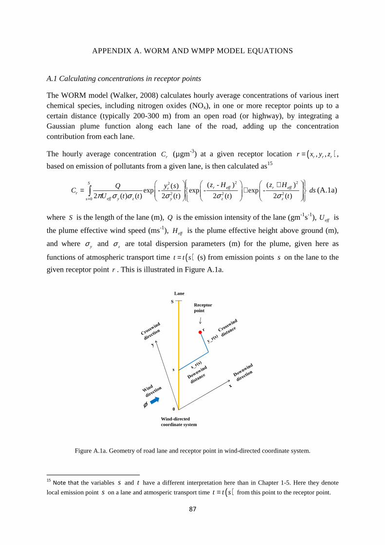
87

APPENDIX A. WORM AND WMPP MODEL EQUATIONS

A.1 Calculating concentrations in receptor points

The WORM model (Walker, 2008) calculates hourly average concentrations of various inert chemical species, including nitrogen oxides (NOx), in one or more receptor points up to a certain distance (typically 200-300 m) from an open road (or highway), by integrating a Gaussian plume function along each lane of the road, adding up the concentration contribution from each lane.

The hourly average concentration rC (µgm-3) at a given receptor location ( ), ,r r rr x y z= ,

based on emission of pollutants from a given lane, is then calculated as15

2 22

2 2 20

( - ) ( )( )exp - exp - exp -

2 ( ) ( ) 2 ( ) 2 ( ) 2 ( )

Sr eff r effr

reff y z y z zs

z H z Hy sQC ds

U t t t t tπ σ σ σ σ σ=

+ = +

∫ (A.1a)

where S is the length of the lane (m), Q is the emission intensity of the lane (gm-1s-1), effU is

the plume effective wind speed (ms-1), effH is the plume effective height above ground (m),

and where yσ and zσ are total dispersion parameters (m) for the plume, given here as

functions of atmospheric transport time ( )t t s= (s) from emission points s on the lane to the

given receptor point r . This is illustrated in Figure A.1a.

Figure A.1a. Geometry of road lane and receptor point in wind-directed coordinate system.

15

Note that the variables s and t have a different interpretation here than in Chapter 1-5. Here they denote

local emission point s on a lane and atmosperic transport time ( )t t s= from this point to the receptor point.

S

0

s

Receptor point

Lane

Wind-directed coordinate system

ϕ

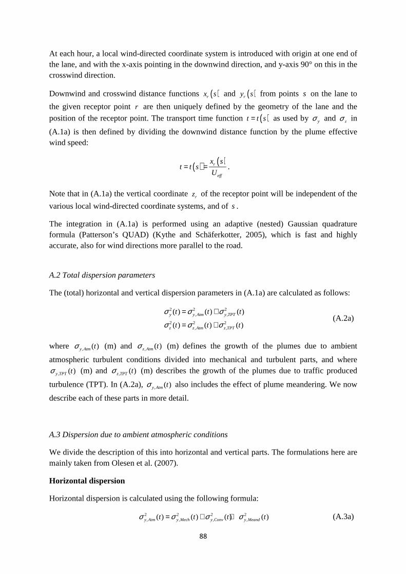
88

At each hour, a local wind-directed coordinate system is introduced with origin at one end of the lane, and with the x-axis pointing in the downwind direction, and y-axis 90° on this in the crosswind direction.

Downwind and crosswind distance functions ( )rx s and ( )ry s from points s on the lane to

the given receptor point r are then uniquely defined by the geometry of the lane and the

position of the receptor point. The transport time function ( )t t s= as used by yσ and zσ in

(A.1a) is then defined by dividing the downwind distance function by the plume effective wind speed:

( ) ( )r

eff

x st t s

U= = .

Note that in (A.1a) the vertical coordinate rz of the receptor point will be independent of the

various local wind-directed coordinate systems, and of s .

The integration in (A.1a) is performed using an adaptive (nested) Gaussian quadrature formula (Patterson’s QUAD) (Kythe and Schäferkotter, 2005), which is fast and highly accurate, also for wind directions more parallel to the road. A.2 Total dispersion parameters

The (total) horizontal and vertical dispersion parameters in (A.1a) are calculated as follows:

2 2 2

, ,

2 2 2, ,

( ) ( ) ( )

( ) ( ) ( )

y y Atm y TPT

z z Atm z TPT

t t t

t t t

σ σ σ

σ σ σ

= +

= + (A.2a)

where , ( )y Atm tσ (m) and , ( )z Atm tσ (m) defines the growth of the plumes due to ambient

atmospheric turbulent conditions divided into mechanical and turbulent parts, and where

, ( )y TPT tσ (m) and , ( )z TPT tσ (m) describes the growth of the plumes due to traffic produced

turbulence (TPT). In (A.2a), , ( )y Atm tσ also includes the effect of plume meandering. We now

describe each of these parts in more detail.

A.3 Dispersion due to ambient atmospheric conditions

We divide the description of this into horizontal and vertical parts. The formulations here are mainly taken from Olesen et al. (2007).

Horizontal dispersion

Horizontal dispersion is calculated using the following formula:

2 2 2 2, , , ,( ) ( ) ( ) ( )y Atm y Mech y Conv y Meandt t t tσ σ σ σ= + + (A.3a)

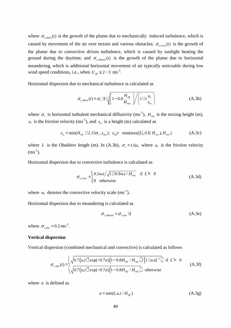
89

where , ( )y Mech tσ is the growth of the plume due to mechanically induced turbulence, which is

caused by movement of the air over terrain and various obstacles; , ( )y Conv tσ is the growth of

the plume due to convective driven turbulence, which is caused by sunlight heating the ground during the daytime; and , ( )y Meand tσ is the growth of the plume due to horizontal

meandering, which is additional horizontal movement of air typically noticeable during low wind speed conditions, i.e., when 2 3effU ≤ − ms-1.

Horizontal dispersion due to mechanical turbulence is calculated as

*, ( ) 1 0.8 1eff

y Mech vmix m

H ut t t

H zσ σ

= ⋅ ⋅ − +

(A.3b)

where vσ is horizontal turbulent mechanical diffusivity (ms-1), mixH is the mixing height (m),

*u is the friction velocity (ms-1), and mz is a height (m) calculated as

lim limmin( 2.15 , ); min(max( ,0.1 ), )m eff z mix mixz H z z L H Hσ= + = ⋅ (A.3c)

where L is the Obukhov length (m). In (A.3b), *1.6v uσ = where *u is the friction velocity

(ms-1).

Horizontal dispersion due to convective turbulence is calculated as

1

* *,

0.5 1 0.9 / if 0

0 otherwisemix

y Conv

w t w t H Lσ− + <=

(A.3d)

where *w denotes the convective velocity scale (ms-1).

Horizontal dispersion due to meandering is calculated as

, ,miny Meand v tσ σ= ⋅ (A.3e)

where ,min 0.2vσ = ms-1.

Vertical dispersion

Vertical dispersion (combined mechanical and convective) is calculated as follows

( ) ( ) ( )( ) ( )

2 1 1* *

,2

*

0.7 exp( 0.7 ) 1 0.8 / / 1 if 0( )

0.7 exp( 0.7 ) 1 0.8 / otherwise

eff mix

z Atm

eff mix

u t a H H u tL Lt

u t a H Hσ

− − − − + >= − −

(A.3f)

where a is defined as

*min(1, / )effa u t H= (A.3g)

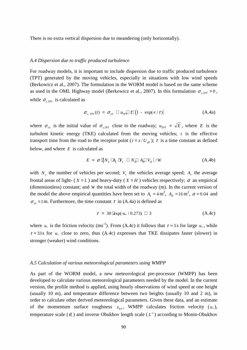
90

There is no extra vertical dispersion due to meandering (only horizontally).

A.4 Dispersion due to traffic produced turbulence

For roadway models, it is important to include dispersion due to traffic produced turbulence (TPT) generated by the moving vehicles, especially in situations with low wind speeds (Berkowicz et al., 2007). The formulation in the WORM model is based on the same scheme as used in the OML Highway model (Berkowicz et al., 2007). In this formulation , 0y TPTσ = ,

while ,z TPTσ is calculated as

( ), 0( ) 1 - exp(- / )z TPT z TPTt u tσ σ τ τ= + ⋅ ⋅ (A.4a)

where 0zσ is the initial value of ,z TPTσ close to the roadway; TPTu E= , where E is the

turbulent kinetic energy (TKE) calculated from the moving vehicles; t is the effective transport time from the road to the receptor point ( / efft x U= ); τ is a time constant as defined

below, and where E is calculated as

( ) /L L L H H HE N A V N A V Wα= ⋅ ⋅ ⋅ + ⋅ ⋅ (A.4b)

with xN the number of vehicles per second; xV the vehicles average speed; xA the average

frontal areas of light- (X L= ) and heavy-duty (X H= ) vehicles respectively; α an empirical (dimensionless) constant; and W the total width of the roadway (m). In the current version of the model the above empirical quantities have been set to 4LA = m2, 16HA = m2, 0.04α = and

0 1zσ = m. Furthermore, the time constant τ in (A.4a) is defined as

* 30 exp(- / 0.273) 3uτ = ⋅ + (A.4c)

where *u is the friction velocity (ms-1). From (A.4c) it follows that 3τ ≈ s for large *u , while

33τ ≈ s for *u close to zero, thus (A.4c) expresses that TKE dissipates faster (slower) in

stronger (weaker) wind conditions.

A.5 Calculation of various meteorological parameters using WMPP

As part of the WORM model, a new meteorological pre-processor (WMPP) has been developed to calculate various meteorological parameters needed by the model. In the current version, the profile method is applied, using hourly observations of wind speed at one height (usually 10 m), and temperature difference between two heights (usually 10 and 2 m), in order to calculate other derived meteorological parameters. Given these data, and an estimate of the momentum surface roughness 0mz , WMPP calculates friction velocity (*u ),

temperature scale (*θ ) and inverse Obukhov length scale (1L− ) according to Monin-Obukhov

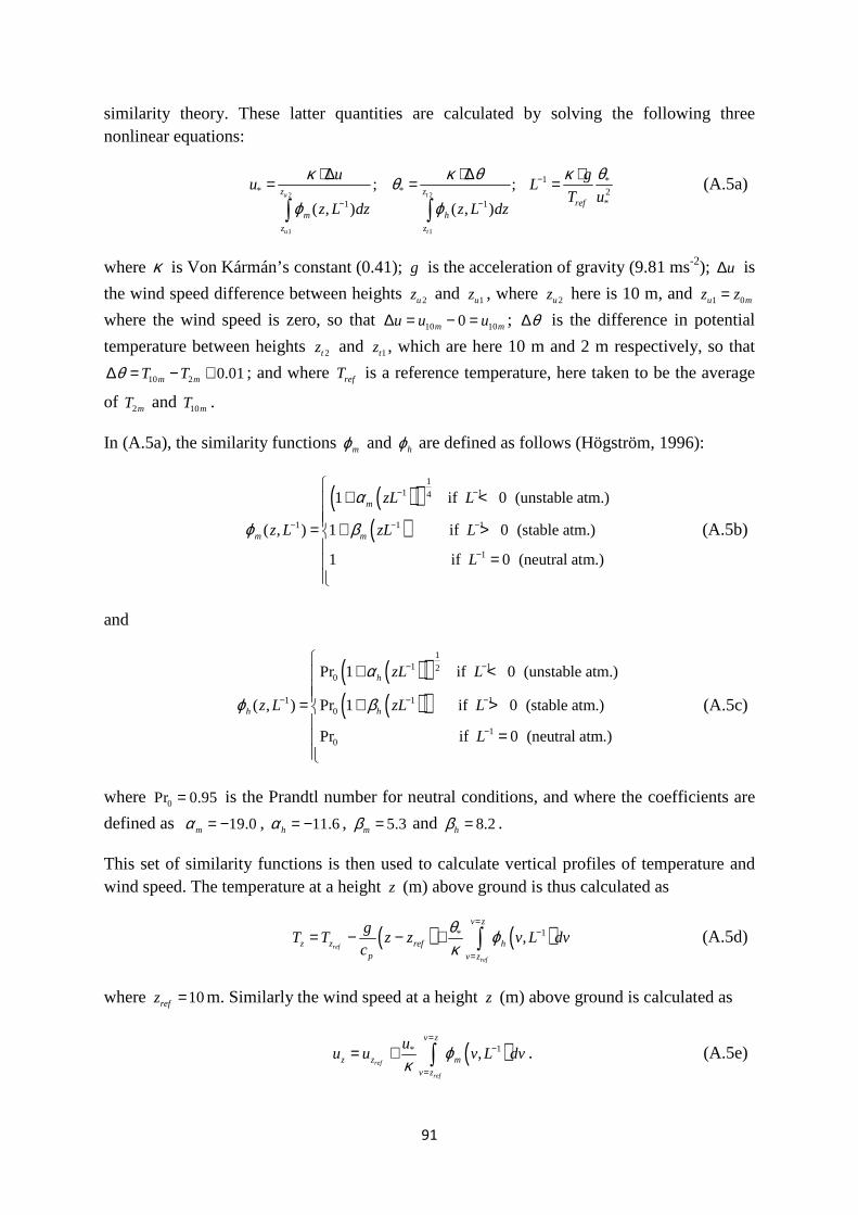
91

similarity theory. These latter quantities are calculated by solving the following three nonlinear equations:

2 2

1 1

1 ** * 2

*1 1

; ;

( , ) ( , )u t

u t

z zref

m h

z z

u gu L

T uz L dz z L dz

θκ κ θ κθϕ ϕ

−

− −

⋅ ∆ ⋅ ∆ ⋅= = =

∫ ∫ (A.5a)

where κ is Von Kármán’s constant (0.41); g is the acceleration of gravity (9.81 ms-2); u∆ is

the wind speed difference between heights 2uz and 1uz , where 2uz here is 10 m, and 1 0u mz z=

where the wind speed is zero, so that 10 100m mu u u∆ = − = ; θ∆ is the difference in potential

temperature between heights 2tz and 1tz , which are here 10 m and 2 m respectively, so that

10 2 0.01m mT Tθ∆ = − + ; and where refT is a reference temperature, here taken to be the average

of 2mT and 10mT .

In (A.5a), the similarity functions mϕ and hϕ are defined as follows (Högström, 1996):

( )( )( )

11 14

1 1 1

1

1 if 0 (unstable atm.)

( , ) 1 if 0 (stable atm.)

1 if 0 (neutral atm.)

m

m m

zL L

z L zL L

L

α

ϕ β

−− −

− − −

−

+ <

= + >

=

(A.5b)

and

( )( )( )( )

11 12

0

1 1 10

10

Pr 1 if 0 (unstable atm.)

( , ) Pr 1 if 0 (stable atm.)

Pr if 0 (neutral atm.)

h

h h

zL L

z L zL L

L

α

ϕ β

−− −

− − −

−

+ <

= + >

=

(A.5c)

where 0Pr 0.95= is the Prandtl number for neutral conditions, and where the coefficients are

defined as 19.0mα = − , 11.6hα = − , 5.3mβ = and 8.2hβ = .

This set of similarity functions is then used to calculate vertical profiles of temperature and wind speed. The temperature at a height z (m) above ground is thus calculated as

( ) ( )1* ,ref

ref

v z

z z ref hp v z

gT T z z v L dv

c

θ ϕκ

=−

=

= − − + ∫ (A.5d)

where 10refz = m. Similarly the wind speed at a height z (m) above ground is calculated as

( )1* ,ref

ref

v z

z z m

v z

uu u v L dvϕ

κ

=−

=

= + ∫ . (A.5e)

92

The convective velocity scale *w (ms-1) is calculated as

11 3

1* * if 0 (unstable atm.)mixH L

w u Lκ

−− −= <

(A.5f)

and is only applied for unstable atmospheric conditions.

Finally, the mixing height mixH (m) is calculated as

( )

1*

1 1*1

0.3 if 0 (unstable and neutral atm.)

11 2.28 if 0 (stable atm.)

3.8

cor

mix

cor

u f LH

u L f LL

−

− −−

≤=

+ >

(A.5g)

where corf is the Coriolis parameter. This latter parameter is calculated as 2 sincorf θ= Ω ⋅ ,

where Ω is the angular speed of rotation of the Earth, i.e. 2 / sidTπΩ = , with sidT the sidereal

period of rotation, i.e., 23 60 60 56 60 4.1sidT = ⋅ ⋅ + ⋅ + (s), and where θ is the site latitude (60°).

For more details of these, and other recommended schemes, see the final reports from the COST 710 project (Fisher et al., 1998) and Högström (1996).

Minimum values can be defined for some of the meteorological parameters in the WORM model such as the effective wind speed, Obukhov length, mixing height and horizontal and vertical diffusivities. Table A.5a gives an overview of the minimum values set for these parameters as has been used in the present calculations at Nordbysletta.

Table A.5a. Minimum values for some of the meteorological parameters used by WORM.

Parameter Minimum value effU No lower limit, i.e., 0 ms-1

L 10 m

mixH 10 m

vσ 0.2 ms-1

wσ No lower limit, i.e., 0 ms-1

93

APPENDIX B. ADAPTIVE RANDOM-WALK METROPOLIS-WITHIN-GIBBS FOR MODEL C

B.1 Conditional distributions

Using the original nomenclature from Section 2.3.4, model C equations for a given observation point ms s= can be written

( ) ( ) ( )0log , log , ,m c m mc s t f s t s tβ ε= + + (B.1a)

where

( ) ( ) ( ) ( ) ( )2, , 1 , ; , 0,m m m ms t s t s t s t Nε φε η η σ= − + ∼ (B.1b)

and where the observation equation is

( ) ( ) ( ) ( ) ( )2log , log , , ; , 0,m m y m y m yy s t c s t s t s t Nη η σ= + ∼ . (B.1c)

By inserting ( ),ms tε from (B.1a) into (B.1b) we obtain

( ) ( ) ( ) ( )( ) ( )0 0log , log , log , 1 log , 1 ,m c m m c m mc s t f s t c s t f s t s tβ φ β η− − = − − − − + .

If we define state variables tx as

( ) ( )log , log ,t m c mx c s t f s t= −

and replace ( ),my s t , ( ),ms tη , ( ),y ms tη and ( ),c mf s t with ty , tη , ,y tη and tf , respectively,

equations (B.1a-c) can alternatively be written

( ) ( )20 1 0 ; 0,t t t tx x Nβ φ β η η σ−− = − + ∼ (B.1d)

( )2, ,log log ; 0,t t t y t y t yy x f Nη η σ= + + ∼ . (B.1e)

Using these equations with initial state 0 0x β= , and priors for the parameters 0β , φ and 2τ σ −= as defined in Section 2.3.4, it can be shown (not shown here) that the conditional

posterior distributions of these parameters can be given analytically as follows16:

( )( )

( ) ( )1

10 1: 1: 2

1| , , , ,

1 1

T

t tt

T T

x xp x y N

T T

φβ φ τ

φ τ φ

−=

− =

− −

∑

and

16

T here is the same as 'T in Section 2.3.4.

94

( )( )( )

( ) ( )

0 1 01

1: 1: 02 2

0 01 1

1| , , , ,

T

t tt

T T T T

t tt t

x xp x y N

x x

β βφ β τ

β τ β

−=

= =

− − = − −

∑

∑ ∑

and

( ) ( )( )1

2

1: 1: 0 0 11

1 1 1| , , , Gamma ,

2 2

T

T T t tt

p x y a T x xb

τ β φ β φ µ−

−=

= + + − − − ∑

with parameters 14.98a = (shape) and 0.14b = (scale) from the prior Gamma-distribution for τ as given in Section 2.3.4. In these expressions, we have used the short-hand notation

( )1: 1,...,T Tx x x= and ( )1: 1,...,T Ty y y= .

Furthermore, it can be shown (not shown here) that the conditional posterior distribution of state variable tx can be written

( )

( )( ) ( )( )( ) ( )1: 1 1: 1: 0

2 2

0 1 0 1 0 0

| , , , , ,

exp 0.5 0.5 |

t t t T T

t t t t t t

p x x x y

x x x x p y x

β φ τ

β φ β β φ β

− +

− +

∝

− − − − − − − − ⋅

where the observational likelihood ( )|t tp y x is obtained directly from (B.1e), i.e.,

( )2

log log1| exp

2t t t

t ty

y x fp y x

σ

− − ∝ −

with yσ being the observational error standard deviation.

B.2 Adaptive random-walk Metropolis-within-Gibbs

Based on the development in the previous section, and the general theory of Gibbs sampling as described in Section 3.3., an adaptive random-walk Metropolis-within-Gibbs (AdapRWMwG) algorithm for model C can be defined as follows:

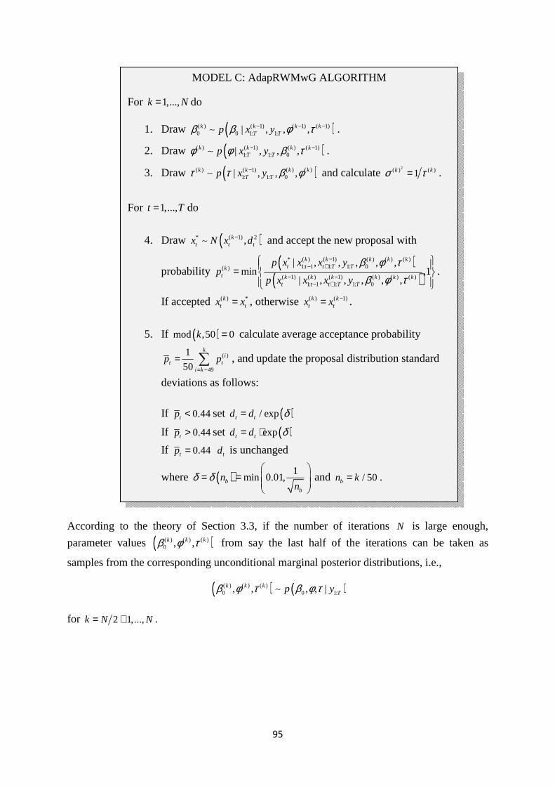
95

According to the theory of Section 3.3, if the number of iterations N is large enough,

parameter values ( )( ) ( ) ( )0 , ,k k kβ φ τ from say the last half of the iterations can be taken as

samples from the corresponding unconditional marginal posterior distributions, i.e.,

( ) ( )( ) ( ) ( )0 0 1:, , , , |k k k

Tp yβ φ τ β φ τ∼

for 2 1,...,k N N= + .

MODEL C: AdapRWMwG ALGORITHM

For 1,...,k N= do

1. Draw ( )( ) ( 1) ( 1) ( 1)0 0 1: 1:| , , ,k k k k

T Tp x yβ β φ τ− − −∼ .

2. Draw ( )( ) ( 1) ( ) ( 1)1: 1: 0| , , ,k k k k

T Tp x yφ φ β τ− −∼ .

3. Draw ( )( ) ( 1) ( ) ( )1: 1: 0| , , ,k k k k

T Tp x yτ τ β φ−∼ and calculate

2( ) ( )1k kσ τ= .

For 1,...,t T= do

4. Draw ( )* ( 1) 2,kt t tx N x d−∼ and accept the new proposal with

probability ( )

( )* ( ) ( 1) ( ) ( ) ( )

1: 1 1: 1: 0( )

( 1) ( ) ( 1) ( ) ( ) ( )1: 1 1: 1: 0

| , , , , ,min ,1

| , , , , ,

k k k k kt t t T Tk

t k k k k k kt t t T T

p x x x yp

p x x x y

β φ τβ φ τ

−− +

− −− +

=

.

If accepted ( ) *kt tx x= , otherwise ( ) ( 1)k k

t tx x −= .

5. If ( )mod ,50 0k = calculate average acceptance probability

( )

49

1

50

ki

t ti k

p p= −

= ∑ , and update the proposal distribution standard

deviations as follows:

If 0.44tp < set ( )/ expt td d δ=

If 0.44tp > set ( )expt td d δ= ⋅

If 0.44tp = td is unchanged

where ( ) 1min 0.01,b

b

nn

δ δ

= =

and / 50bn k= .

97

REFERENCES

AirQUIS. 2005. Emissions module. Norwegian Institute for Air Research. http://www.nilu.no.

Bai Y. 2009. Convergence of adaptive Markov Chain Monte Carlo algorithms. Ph.D. Thesis. Department of Statistics, University of Toronto. http://www.utstat.utoronto.ca/~yanbai/.

Bai Y, Roberts GO, Rosenthal JS. 2009. On the containment condition for adaptive Markov Chain Monte Carlo algorithms. Preprint. Department of Statistics, University of Toronto. http://www.utstat.utoronto.ca/~yanbai/.

Bates SC, Cullen A, Raftery AE. 2003. Bayesian uncertainty assessment in multicompartment deterministic simulation models for environmental risk assessment. Environmetrics 14: 355-371.

Bayarri MJ, Berger JO, Paulo R, Sacks J. 2007. A framework for validation of computer models. Technometrics 49(2): 138-154.

Benson P. 1992. A review of the development and application of the CALINE3 and 4 models. Atmospheric Environment 26B: 379-390.

Berger J, Walker SE, Denby B, Berkowicz R, Løfstrøm P, Ketzel M, Härkönen J, Nikmo J, Karppinen A. 2010. Evaluation and inter-comparison of open road line source models currently in use in the Nordic countries. Boreal Environmental Research 15: 319-334.

Berkowicz R, Løfstrøm P, Ketzel M, Jensen SS and Hvidberg M. 2007. OML Highway. Phase 1: Specifications for a Danish Highway Air Pollution Model. National Environmental Research Institute, University of Aarhus, Denmark. 62 pp. – NERI Technical Report No. 633. http://www.dmu.dk/Pub/FR633.pdf.

Blum JR, Hanson DL, Koopmans LH. 1963. On the strong law of large numbers for a class of stochastic processes, Z. Wahrsch. Ver. Geb. 2: 1-11.

Box GEP, Cox DR. 1964. An analysis of transformations (with discussion). Journal of the Royal Statistical Society B 26: 211-252.

Bremnes JB. 2004. Probabilistic forecasts of precipitation in terms of quantiles using NWP model output. Monthly Weather Review 132: 338-347.

Campbell K. 2006. Statistical calibration of computer simulations. Reliability Engineering and System Safety 91: 1358-1363.

Casati B, Wilson LJ, Stephenson DB, Nurmi P, Ghelli A, Pocernich M, Damrath U, Ebert EE, Brown BG, Mason S. 2008. Review forecast verification: current status and future directions. Meteorological Applications 15: 3-18.

Chatwin PC. 1982. The use of statistics in describing and predicting the effects of dispersing gas clouds. Journal on Hazardous Materials 6: 213-230.

Colvile RN, Woodfield NK, Carruthers DJ, Fisher BEA, Rickard A, Neville S, Hughes A. 2002. Uncertainty in dispersion modelling and urban air quality mapping. Environmental Science & Policy 5: 207-220.

Dabberdt WF, Miller E, Uncertainty, ensembles and air quality dispersion modelling: applications and challenges. 2000. Atmospheric Environment 34(27): 4667-4673(7).

Davenport AG, Grimmond CSB, Oke TR, Wieringa J. 2000. Estimating the roughness of cities and sheltered country. Preprints of the AMS 12th Conference on Applied Climatology, 96-99.

98

EU. 2006. CAFE reference documents. http://ec.europa.eu/environment/archives/cafe/general/keydocs.htm.

Fisher BEA., Erbrink JJ, Finardi S, Jeannet P, Joffre S, Morselli MG, Pechinger U, Seibert P, Thomson DJ. 1998. COST Action 710 – Final report. Harmonisation of the pre-processing of meteorological data for atmospheric dispersion models. EUR 18195. Luxembourg: Office for Official Publications of the European Communities, 431.

Fuentes M, Raftery AE. 2005. Model evaluation and spatial interpolation by Bayesian combination of observations with outputs from numerical models. Biometrics 61(1): 36-45.

Gelman A, Carlin JB, Stern HS, Rubin DB. 2004. Bayesian Data Analysis (2nd ed.), Chapman & Hall/CRC: London.

Gidhagen L, Kyrklund T, Johansson H. 2005. SIMAIR: Model för beräkning av luftkvalitet i vägars närområde – slutrapport mars 2005. SMHI rapport nr. 2005-37 (in Swedish).

Gneiting T, Balabdaoui, F, Raftery AE. 2007a. Probabilistic forecasts, calibration and sharpness. Journal of the Royal Statistical Society B 69-2: 243-268.

Gneiting T, Raftery AE. 2007b. Strictly proper scoring rules, prediction and estimation. Journal of the American Statistical Association 122(477), 359-378.

Goldstein M, Rougier J. 2008. Reified Bayesian modelling and inference for physical systems. Journal of Statistical Planning and Inference 139: 1221-1239.

Hagen LO, Larssen S, Walker SE. 2003. Forurensning som funksjon av avstand fra vei. Målinger på RV 159 Nordby-sletta v/Skårer vinteren 2001-2002, og sammenligning med VLUFT. Kjeller, Norwegian Institute for Air Research, NILU OR 22/2003 (in Norwegian).

Hersbach H. 2000. Decomposition of the continuous ranked probability score for ensemble prediction systems. Weather and Forecasting 15: 559-570.

Härkönen J, Valkonen E, Kukkonen J, Rantakrans E, Lahtinen K, Karppinen A, Jalkanen L. 1996. A model for the dispersion of pollution from a road network. Publications on Air Quality 23, Finnish Meteorological Institute, Helsinki.

Higdon D, Gattiker J, Williams B, Rightley M. 2008. Computer model calibration using high-dimensional output. Journal of the American Statistical Association 103(482): 570-583.

Hogrefe C, Rao ST. 2001. Demonstrating attainment of the air quality standards: Integration of observations and model predictions into the probabilistic framework. Journal of Air and Waste Management Association 51: 1060-1072.

Högström U. 1996. Review of some basic characteristics of the atmospheric surface layer. Boundary-Layer Meteorology 78: 215-246.

Irwin JS, Petersen WB, Howard SC. 2007. Probabilistic characterization of atmospheric transport and diffusion. Journal of Applied Meteorology and Climatology 46: 980 – 993.

Joliffe IT, Stephenson DB (eds.). 2003. Forecast Verification: A Practitioner’s Guide in Atmospheric Science, John Wiley & Sons, Ltd.: Chichester, West Sussex, England.

Kennedy MC, O’Hagan A. 2001. Bayesian calibration of computer models. Journal of the Royal Statistical Society B 63: 425-450.

Kurowicka D, Cooke R. 2006. Uncertainty Analysis with High Dimensional Dependence Modelling. John Wiley & Sons, Ltd: Chichester, West Sussex, England.

99

Kythe PK, Schäferkotter MR. 2005. Handbook of Computational Methods for Integration. Chapman & Hall/CRC, 598.

Le NH, Zidek JV. 2006. Statistical Analysis of Environmental Space-Time Processes. Springer: New York.

Lewellen WS, Sykes RI. 1989. Meteorological data needs for modeling air quality uncertainties. Journal of Atmospheric.and Oceanic Technology 6: 759-768.

Nafstad P, Håheim LL, Wisløff T, Gram F, Oftedal B, Holme I, Hjermann I, Leren P. 2004. Urban air pollution and mortality in a cohort of Norwegian men. Environmental Health Perspective, 112(5).

Oftedal B, Brunekreef B, Nystad W, Madsen C, Walker SE, Nafstad P. 2008. Residential outdoor air pollution and lung function in schoolchildren. Epidemiology 19: 129-137.

Olesen HR, Berkowicz R, Løfstrøm P. 2007. OML: Review of model formulation. National Environmental Research Institute, University of Aarhus, Denmark. 130 pp. – NERI Technical Report No. 609, http://www.dmu.dk/Pub/FR609.pdf.

O’Hagan A. 2006. Bayesian analysis of computer code outputs: A tutorial. Reliability Engineering and System Safety 91: 1290-1300.

Patton A, Politis DN, White H. 2009. Correction to “Automatic block-length selection for the dependent bootstrap by D. Politis and H. White”. Econometric Reviews 28(4): 372-375.

Petersen WB. 1980. User’s Guide for HIWAY-2. A highway air pollution model. EPA-600/8-80-018. U.S. EPA, Research Triangle Park, NC.

Pinder RW, Gilliam RC, Appel KW, Napelenok SL, Foley KM, Gilliland AB. 2009. Efficient probabilistic estimates of surface ozone concentration using an ensemble of model configurations and direct sensitivity calculations. Environmental Science & Technology 43: 2388-2393.

Politis DN, White H. 2004. Automatic block-length selection for the dependent bootstrap. Econometric Reviews 23(1): 53-70.

Rao KS. 2005. Uncertainty analysis in atmospheric dispersion modelling. Pure and applied geophysics 162: 1893-1917.

Robert CP, Casella G. 2004. Monte Carlo Statistical Methods (2nd ed.), Springer: New York.

Roberts GO, Rosenthal JS. 2009. Examples of adaptive MCMC. Journal of Computational and Graphical Statistics 18(2): 349-367.

Roberts GO, Rosenthal JS. 2007. Coupling and ergodicity of adaptive Markov Chain Monte Carlo algorithms. Journal of Applied Probability 44: 458-475.

Rosenthal JS. 2010. Optimal proposal distributions and adaptive MCMC. Chapter for MCMC handbook, S. Brooks, A. Gelman, G. Jones and X.-L- Meng, eds. http://www.probability.ca/jeff/.

Shaddick G, Lee D, Zidek JV, Salway R. 2008. Estimating exposure response functions using ambient pollution concentrations. Annals of Applied Statistics 2(4): 1249-1270.

Shaddick G, Zidek J, Lee D, White R, Meloche J, Chatfield C. 2006a. Using a probabilistic model (pCNEM) to estimate personal exposure to air pollution in a study of the short-term effect of PM10 on mortality. University of Bath online publications store – OpuS, UK. http://opus.bath.ac.uk/7025.

100

Shaddick G, Kounali D, Briggs D, Beelan R, Hoek G, Hoogh CDE, Pebesma E, Vienneau D. 2006b. Using Bayesian hierarchical modelling to produce high resolution maps of air pollution in the EU. University of Bath online publications store – OpuS, UK. http://opus.bath.ac.uk/7026.

Sharma N, Chaudry KK, Chalapati Rao CV. 2004. Vehicular pollution prediction modeling: a review of highway dispersion models. Transport Reviews 24: 409-435.

Shumway RH, Stoffer DS. 2006. Time Series Analysis and Its Applications. With R Examples (2nd ed.), Springer: New York.

Tønnesen D. 2010. Personal communication. Norwegian Institute for Air Research (NILU).

Tørnkvist KK. 2006. Personal communication. Norwegian Institute for Air Research (NILU).

Vardoulakis S, Fisher BEA, Gonzalez-Flescha N, Pericleous K. 2002. Model sensitivity and uncertainty analysis using roadside air quality measurements. Atmospheric Environment 36(13): 2121-2134.

Walker SE. 2008. WORM – A new open road line source model for low wind speed conditions. Proceedings from the “12th International Conference on Harmonisation within Atmospheric Dispersion Modelling for Regulatory Purposes”. Cavtat, Croatia, October 6-9, 2008. http://www.harmo.org.

Walker SE. 2007. Quantification of uncertainties associated with an integrated Gaussian line source model using ensembles. Proceedings from the “11th International Conference on Harmonisation within Atmospheric Dispersion Modelling for Regulatory Purposes”. Cambridge, UK, July 2-5, 2007. http://www.harmo.org.

Walker SE, Berger J. 2007. Application of data assimilation in open road line source modelling, 6th International Conference on Urban Air Quality. Cyprus, March 27-29, 2007.

Walker SE, Gjerstad KI, Berger J. 2006. Air4EU – Case Study D7.1.4. Data assimilation in open road line source modelling. http://www.air4eu.nl.

WHO. 2006a. Air Quality Guidelines. Global update 2005. Particulate matter, ozone, nitrogen dioxide and sulphur dioxide. http://www.euro.who.int/InformationSources/Publications/Catalogue/20070323_1.

WHO. 2006b. Health risks of particulate matter from long-range transboundary air pollution. World Health Organization. Regional Office for Europe. Copenhagen.

WHO. 2004. Comparative quantification of health risks: global and regional burden of disease attributable to selected major risk factors. Ezzati M et al. (eds.) World Health Organization, 2004.

Wikle CK, Berliner LM. 2007. A Bayesian tutorial for data assimilation. Physica D: Nonlinear Phenomena 230(1-2): 1-16.

Wilks DS. 2006. Statistical Methods in the Atmospheric Sciences (2nd ed.), Academic Press: London.

Zidek JV, Shaddick G, White R, Meloche J, Chatfield C. 2005. Using a probabilistic model (pCNEM) to estimate personal exposure to air pollution. Environmetrics 16(5): 481-493.

PROBABILISTIC MODELLING OF AIR POLLUTION FROM ROAD TRAFFIC

Documents

Transcript of PROBABILISTIC MODELLING OF AIR POLLUTION FROM ROAD TRAFFIC