Probabilistic Clustering of Extratropical Cyclones Using...

Probabilistic Clustering of Extratropical Cyclones

Using Regression Mixture Models

Scott J. Gaffney1, Andrew W. Robertson2∗, Padhraic Smyth3,

Suzana J. Camargo2 and Michael Ghil4,5

1Data Mining Research, Yahoo! Inc.,

Sunnyvale, CA, USA2International Research Institute for Climate and Society (IRI),

The Earth Institute at Columbia University, Palisades, NY, USA3Department of Computer Science,

University of California, Irvine, CA, USA4Department of Atmospheric and Oceanic Sciences and IGPP,

University of California, Los Angeles, CA5Additional affiliation: Departement Terre-Atmosphere-Ocean

and Laboratoire de Meteorologie Dynamique (CNRS and IPSL),

Ecole Normale Superieure, Paris, France.

December 22, 2006

Climate Dynamics, sub judice

∗Corresponding author: Dr. Andrew W. Robertson, IRI - Monell 230, 61 Route 9W, Palisades, NY 10964. Phone:+1 845 680 4491, Fax: +1 845 680 4865, E-mail: [email protected].

1

Abstract

A probabilistic clustering technique is developed for classification of wintertime

extratropical cyclone (ETC) tracks over the North Atlantic. We use a regression mix-

ture model to describe the longitude-time and latitude–time propagation of the ETCs.

A simple tracking algorithm is applied to 6-hourly mean sea-level pressure fields to

obtain the tracks from either a general circulation model (GCM) or a reanalysis data

set. Quadratic curves are found to provide the best description of the data.

We select a three-cluster classification for both data sets, based on a mix of objec-

tive and subjective criteria. The track orientations in each of the clusters are broadly

similar for the GCM and reanalyzed data; they are characterized by predominantly

south-to-north (S–N), west-to-east (W–E), and southwest-to-northeast (SW–NE) track-

ing cyclones, respectively. The reanalysis cyclone tracks, however, are found to be

much more tightly clustered geographically than those of the GCM. For the reanalysis

data, a link is found between the occurrence of cyclones belonging to different clusters

of trajectory-shape, and the phase of the North Atlantic Oscillation (NAO). The pos-

itive phase of the NAO is associated with the SW–NE oriented cluster, whose tracks

are relatively straight and smooth (with cyclones that are typically faster, more intense,

2

and of longer duration). The negative NAO phase is associated with more-erratic W–E

tracks, with typically weaker and slower-moving cyclones. The S–N cluster is accom-

panied by a more transient geopotential trough over the western North Atlantic. No

clear associations are found in the case of the GCM composites.

The GCM is able to capture cyclone tracks of quite realistic orientation, as well

as subtle associated features of cyclone intensity, speed and lifetimes. The clustering

clearly highlights, though, the presence of serious systematic errors in the GCM’s

simulation of ETC behavior.

3

1. Introduction

a. Background and motivation

Wintertime extratropical cyclones (ETCs) are responsible for severe-weather events with high

winds and/or flooding over North America and western Europe; they caused the second largest

insurance loss due to weather (after hurricanes) during the period 1990–98 (Saunders 1999). On

the other hand they are also the primary source of wintertime precipitation and total water resources

for much of the western United States.

ETCs play a special role as intermediaries between large-scale climate dynamics and local

impacts: they are crucial dynamical ingredients of the atmospheric circulation, while at the same

time directly impacting local weather. ETCs constitute an important nexus between the potentially

predictable large-scale components of climate, such as certain hemispheric or sectorial atmospheric

teleconnection patterns associated with internal climate variability (Lau 1988; Robertson and Metz

1990) or with global warming (Fyfe 2003), on the one hand, and societally important weather

events (MunichRe 2002), on the other. A better understanding of the behavior of ETCs in the

context of climate variability and change could have important societal implications.

ETCs have localized coherent spatial structures that generally propagate toward the east and

4

go through a well-defined lifecycle (Simmons and Hoskins 1978). Their population is thus most

naturally described as a set of moving objects that follow various tracks and have differing indi-

vidual lifecycle characteristics; this corresponds to a Lagrangian description in fluid dynamical-

terminology. By contrast, most data analysis in the atmospheric sciences has been based on

calculating Eulerian statistics on spatially fixed grids, often using principal component analysis

(Preisendorfer 1988; von Storch and Zwiers 1999) to derive the leading patterns of spatio-temporal

variability. These methods are poorly suited to cyclone trajectories, which are inherently localized

in space in any given time-frame.

The analysis of large sets of ETC trajectories, whether from multi-decadal observed data sets

or from potentially much longer general circulation model (GCM) simulations requires a different

approach. Cluster analysis provides a natural way to analyze sets of trajectories and their relation-

ships with the larger-scale atmospheric circulation, by decomposing large sets of trajectories into

subgroups with homogeneous spatio-temporal characteristics.

In this paper, we use curve-based mixture modeling techniques to perform probabilistic cluster-

ing of ETC trajectories in latitude–longitude space. Curve-based mixture modeling can be viewed

as a particular clustering technique within the broader statistical framework of functional data anal-

ysis (Ramsay and Silverman 1997, 2002). An identification and tracking methodology is devel-

5

oped to produce cyclone trajectories; these trajectories are then clustered using a novel probabilistic

technique based on mixtures of regression models.

We develop and test the tracking and clustering methodology using a 15-winter GCM-generated

mean sea level pressure (MSLP) data set. We then apply the methodology to a 44-year set of reanal-

ysis data. Since the latter is a data assimilation of both meteorological observations and 6-hourly

model forecasts, there is no guarantee of temporally smooth behavior.

b. Related work

Prior work on cyclone tracking has focused specifically on methods for automated identification

and tracking of cyclones, usually from sea-level pressure data. Identification methods range from

the relatively simple approach of finding minima in the surface pressure field (Le Treut and Kalnay

1990; Konig et al. 1993; Terry and Atlas 1996), or in the 5-point Laplacian thereof, to more com-

plex approaches such as the use of image processing and computer vision techniques (Hodges

1994; Mesrobian et al. 1995; Hodges 1998); the latter approaches often involve other atmospheric

fields such as vorticity (Hoskins and Hodges 2002). These algorithms are usually then coupled

with a tracking scheme to produce a final set of trajectories. Methods proposed for tracking so far

include a number of different schemes: nearest-neighbor search (Blender et al. 1997; Konig et al.

6

1993), numerical prediction schemes with cost-minimizing optimizations (Murray and Simmonds

1991), and feature tracking methods from image analysis that are also based on a cost minimiza-

tion framework (Hodges 1994, 1995). Mailier et al. (2006) combined the tracking algorithms of

Hoskins and Hodges (2002) with a Poisson-based modeling approach to analyze clustering in time

of extratropical cyclone tracks in the Northern Hemisphere.

Blender et al. (1997) introduced the idea of using the K-means clustering algorithm to cluster

ETC trajectories of fixed length. The K-means algorithm iteratively searches for compact clusters

of multidimensional points in d-dimensional Euclidean space (Hartigan and Wong 1978); this

algorithm minimizes within-cluster variance for a given number K of clusters. To apply the K-

means algorithm to cyclone trajectory data, one must first convert the variable-length trajectories

into fixed-dimensional vectors. To do this, Blender et al. (1997) constrained each of their storm

trajectories to be exactly 3 days in length and then concatenated each of the latitude and longitude

measurements to form the vectors on which the K-means algorithm operates. Elsner et al. (2000)

and Elsner (2003) used the K-means algorithm to cluster tropical cyclone trajectories based on the

latitude and longitude locations of storms when they reach specific intensities.

This type of vector-based clustering has limitations when applied directly to trajectories. For

example, the conversion of the time and space measurements into a fixed-dimensional vector-space

7

loses spatio-temporal smoothness information related to the underlying dynamics of the ETC pro-

cess, whereas the mixture-based approach uses trajectory models (for each mixture component)

that are smooth as a function of time. Furthermore, the vector-based approach artificially con-

strains the trajectories to have fixed lengths. The regression-based clustering used in this paper

has been shown to provide systematically better fit and more accurate predictions when used to

cluster variable-length trajectory data, compared to vector-based clustering (Gaffney and Smyth

1999; Gaffney 2004). Allowing for tracks of varying lengths may be of particular significance; for

example, Simmons and Hoskins (1978) identified a lifecycle of about 10 days, much longer than

that assumed by Blender et al. (1997). The approach we propose in this paper for ETC clustering,

namely mixtures of regression models, directly incorporates spatio-temporal smoothness in the

trajectories in the modeling process, and accommodates cyclone trajectories of different lengths.

Hierarchical clustering could also be used in this context by defining a distance between pairs of

trajectories. For example, dynamic time-warping techniques could be used to define a transforma-

tion distance between any curve and another (Wang and Gasser 1997). Both hierarchical clustering

and K-means clustering, however, do not allow for a consistent and systematic approach to prob-

lems such as assessing the predictive performance of a cluster model, model selection, or handling

missing data. In contrast, the probabilistic, regression-based approach to clustering provides a sta-

8

tistical basis to systematically address these issues (Fraley and Raftery 1998, 2002; Smyth 2000;

McLachlan and Peel 2000).

c. Purpose and outline

Our purpose in this paper is threefold: (i) to develop further the methodology for ETC tracking and

classification; (ii) to apply this methodology to North Atlantic ETCs that impact European climate;

and (iii) to evaluate the performance of a typical GCM in simulating the observed ETC clusters.

The paper is organized as follows. Section 2 presents our cyclone identification and tracking

methodology and describes the data sets used in this paper. Section 3 introduces a new curve-based

methodology for ETC clustering in two parts: (i) a brief introduction to finite mixture models; and

(ii) their extension to regression mixture models and the integration of cyclones into this frame-

work. Section 4 presents the clustering results for the GCM data, while the corresponding results

for the reanalysis data set appear in Section 5. The ETC clusters are related to the large-scale

meteorological fields in Section 6, followed by concluding remarks in Section 7.

9

2. Data and Tracking Methodology

a. Data

The GCM data set used for this work was generated by the National Center for Atmospheric Re-

search (NCAR) Community Climate Model (CCM3) (Hack et al. 1998). The model is discretized

in spherical harmonics at a T42 resolution, and forced with observed sea surface temperatures

specified at the lower boundary over the 1980/81–1994/95 period. For the tracking, we used 6-

hourly MSLP fields on the model’s approximate 2.8◦ × 2.8◦ Gaussian grid for extended 6-month

winter months (1 November to 30 April) from 1980 to 1995; in each winter there are thus 181 days.

In this paper we focus on North Atlantic ETCs over the area (30◦N–80◦N, 80◦W–30◦E) shown in

Fig. 1.

[Figure 1 near here, please.]

The reanalysis data set used in Section 5 is the National Centers for Environmental Predic-

tion (NCEP)–NCAR data assimilation of historical observations using a state-of-the-art analy-

sis/forecast system (Kalnay et al. 1996). We use 6-hourly MSLP on a regular latitude-longitude

grid of 2.5◦ × 2.5◦, over the same North Atlantic domain as for the GCM, but for the 44 extended

winter seasons 1958/59–2001/02.

10

To cluster ETC trajectories we must first identify and track them from the MSLP frames. Our

identification and tracking scheme is based on methods already used in this context (Blender

et al. 1997; Konig et al. 1993) and requires relatively few parameters to implement. The track-

ing algorithm we use is quite simple and not intended as a general-purpose tracking algorithm—

nonetheless, we found that it produced reliable results on the data sets used in this paper. We only

give a short description below; the full details can be found in Gaffney (2004).

b. Identifying and tracking cyclones

Cyclones are characterized as well-defined surface-pressure minima and their trajectories have

lengths of a few thousand kilometers. We begin with a minimum-finding procedure to locate

candidate centers of cyclones within each field. In order to distinguish these minima more easily

from larger-scale low-pressure areas, the gridded data were spectrally filtered in space at each

time so as to remove the largest planetary-wave scales; these scales were defined as the first five

global spherical harmonics (Hoskins and Hodges 2002; Anderson et al. 2003). Using bicubic

interpolation, a cyclone center that may be off-grid is then obtained.

Spurious minima can arise using this procedure, usually in one of two situations: (1) in high-

pressure regions not associated with cyclonic activity; and (2) on the outskirts of a single cyclonic

11

system with an already located central minimum. These spurious minima are automatically iden-

tified and removed from further analysis, by thresholding the MSLP data at a particular pressure

level to form individual low-pressure regions within the data. This thresholding results in con-

tiguous local pixel regions, where each local region corresponds to the estimated spatial extent of

a single candidate cyclone at a specific time. We then reject minima that are located outside the

low-pressure regions and only keep the deepest minimum within each individual local region. The

threshold was defined via trial-and-error to be -17hPa, a subjective choice that produced intuitive

results—the set of tracks obtained are relatively insensitive to small variations in the value of the

threshold (Gaffney 2004). The same threshold value is used for all times t.

Once the valid MSLP minima have been detected at successive 6-hour time intervals, they are

linked together over time to form cyclone tracks. Each valid minimum at time t is linked with the

closest minimum that was detected within a small neighborhood in the MSLP field from t−6 hours.

This search is carried out within ±7◦ long. and ±5◦ lat. These bounds correspond to a maximum

velocity of approximately 92 km/h in longitude and latitude, at 45◦N; in practice such velocities

are hardly, if ever, reached. In the second step, we eliminate tracks shorter than 2.5 days. This

removes many short and noisy tracks that correspond to local small-scale weather disturbances not

usually considered to be synoptic cyclones.

12

Application of this identification and tracking procedure to the MSLP data from CCM3 pro-

duced 614 cyclones of different durations, each with a minimum of 10 time-steps (i.e., at least

2.5 days long). Figure 1 shows a sample of the resulting cyclone tracks, with starting positions

indicated by circles. Figure 2 contains three summary histograms describing the statistical charac-

teristics of the entire set of trajectories. The cyclone tracks have typical durations of 2.5–4 days,

typical velocities of 30–60 km/hr (i.e. 8–16 m/s), and reach typical maximum intensities, defined

as the minimum MSLP reached, of –30 to –50 mb. These values are of the same order as the

statistics derived from tracking observed cyclones in other studies (Hoskins and Hodges 2002).

We use this set of trajectories as input to our clustering algorithm in what follows.


13

3. Clustering methodology

a. Finite mixture models and model-based clustering

In the standard mixture model framework, we model the probability density function (PDF) for a

d-dimensional vector x, as a function of model parameters φ, by the mixture density

p(x|φ) =K∑k

αk pk(x|θk), (1)

in which φ = {α1, . . . , αK ; θ1, . . . , θK}, αk is the k-th component weight, and pk is the k-th

component density with parameter vector θk; for example, K Gaussian densities each with a d-

dimensional mean vector and a d × d covariance matrix. The mixture weights αk sum to one and

are nonnegative. In this manner a finite mixture model is a PDF composed of a weighted average

of component density functions (McLachlan and Peel 2000).

The mixture model framework can be used for data clustering as follows. A data set of n vec-

tors {x1, . . . ,xn} is observed, and is assumed to be a random sample from the underlying mixture

model. Each data vector xi is generated by one of the K components, but the identity of the gener-

ating component is not observed. The parameters for each density component pk(x|θk), as well as

14

the corresponding weights αk, can be estimated from the data using the Expectation-Maximization

(EM) algorithm, a widely used technique for maximum-likelihood parameter estimation with mix-

ture models (Dempster et al. 1977a; McLachlan and Krishnan 1997). From a clustering viewpoint,

the estimated component models, pk(x|θk), 1 ≤ k ≤ K, are interpreted as K clusters, where each

cluster is defined by a PDF in the d-dimensional input space x.

Furthermore, using Bayes rule and Eqn. (1), the probability that x was generated by the kth

cluster (or component) can be calculated (Eqn. (A2 in Appendix A). These membership probabili-

ties reflect the a posteriori uncertainty (given the data and the model) about which cluster each data

vector xi originated from. A “hard” clustering of the original data {x1, . . . ,xn} can be inferred

by assigning each vector xi to the cluster fk with the highest membership probability, i.e., the

cluster from which it was most likely generated. Finite mixture models have been widely used for

clustering data in this manner in a variety of application areas (e.g., McLachlan and Basford 1988)

including atmospheric sciences (e.g., Smyth et al. 1999; Hannachi and O’Neill 2001; Vrac et al.

2005).

15

b. Cyclone regression mixture models

Regression mixture models are a direct extension of the vector mixture models described above.

For illustration, consider a hypothetical trajectory zi with ni = 4 measurements; the longitude

and latitude measurements are in the first and second column and their initial values have been

subtracted, while ti is the elapsed time from initiation of tracking:

zi =

0 0

1 0.2

2.5 0.4

3.3 0.7

, ti =

0

1

2

3

.

Note that this example represents a cyclone moving mostly in a zonal direction. The methodology

below is developed for the case where each trajectory zi is represented by two-dimensional lat-lon

measurements over time. However, the framework can also handle additional dimensionality in

zi, e.g., 3-dimensional positional vectors could be used to offset distortions introduced by lat-lon

projections, and additional non-positional attributes such as intensity as a function of time could

also be added.

We model longitudinal position with a polynomial regression model of order p in which time

16

ti is the independent variable, e.g., z = βptp +βp−1t

p−1 + . . .+β1t+β0, and likewise for latitude.

Both regression equations can be defined succinctly in terms of the matrix Ti:

zi = Tiβ + εi, εi ∼ N(0, Σ). (2)

Here Ti is the standard ni×(p+1) Vandermonde regression matrix associated with the vector ti; β

is a (p+1)×2 matrix of regression coefficients, which contains the longitude coefficients in the first

column and the latitude coefficients in the second column; and εi is an ni×2 matrix of multivariate

normal errors, with a zero mean and a 2 × 2 covariance matrix Σ. Assuming that the noise term

ε is normal (Gaussian) is equivalent in effect to using a least-squares loss function in regression

fitting. Alternative noise models could also be considered—we used the normal assumption here

since it is the most straightforward computationally and is a common choice for additive noise in

regression models.

The Vandermonde regression matrix Ti consists of (p+1) columns of ti so that the components

of ti in the m-th column are taken to the power of m for 0 ≤ m ≤ p. For example, if p = 2 and

17

ti = (0, 1, 2, 3)′, where ()′ denotes the transpose, then

Ti =

0 0 0

1 1 1

1 2 4

1 3 9

.

The covariance matrix Σ contains three distinct elements: the noise variances σ21 and σ2

2 for

each longitude and latitude measurement, respectively, and the cross-covariance σ12 = σ21 between

any two longitude and latitude measurements. For simplicity, we make the assumption that Σ =

diag(σ21, σ2

2), so that latitude and longitude measurement noise terms are treated as conditionally

independent given the model. While a non-diagonal covariance matrix would allow for modeling

of dependence between the latitude and longitude measurement noise terms, this level of detailed

modeling did not appear necessary for the purposes of clustering and, thus, we used a diagonal

covariance assumption as a simpler alternative.

The conditional density for the i-th cyclone is thus defined as

p(zi|ti, θ) = f(zi|Tiβ, Σ) (3)

18

= (2π)−ni |Σ|−ni/2 exp{−1

2tr

[(zi −Tiβ)Σ−1(zi −Tiβ)′

]},

where the parameter set θ = {β, Σ} contains the regression coefficients β and the noise covariance

matrix Σ.

We can derive regression mixtures for the cyclones by substitution of the unconditional mul-

tivariate density components pk(x|θk) in Eqn. (1) with the conditional regression density compo-

nents pk(z|t, θk), defined in Eqn. (3) above. This results in the following regression mixture model

for ETC trajectories:

p(zi|ti, φ) =K∑k

αk pk(zi|ti, θk) =K∑k

αk fk(zi|Tiβk, Σk). (4)

Note that in this model each ETC is assumed to be generated by one of K different regression

models, and each model has its own “shape” parameters θk = {βk, Σk}. The technique is quite

general and can be adapted to many types of regression models including linear (DeSarbo and Cron

1988), binomial probit (Lwin and Martin 1989), kernel (Gaffney and Smyth 1999), and random

effects (Lenk and DeSarbo 2000; Gaffney and Smyth 2003) models.

19

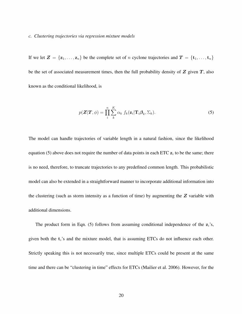
c. Clustering trajectories via regression mixture models

If we let Z = {z1, . . . , zn} be the complete set of n cyclone trajectories and T = {t1, . . . , tn}

be the set of associated measurement times, then the full probability density of Z given T , also

known as the conditional likelihood, is

p(Z|T , φ) =n∏i

K∑k

αk fk(zi|Tiβk, Σk). (5)

The model can handle trajectories of variable length in a natural fashion, since the likelihood

equation (5) above does not require the number of data points in each ETC zi to be the same; there

is no need, therefore, to truncate trajectories to any predefined common length. This probabilistic

model can also be extended in a straightforward manner to incorporate additional information into

the clustering (such as storm intensity as a function of time) by augmenting the Z variable with

additional dimensions.

The product form in Eqn. (5) follows from assuming conditional independence of the zi’s,

given both the ti’s and the mixture model, that is assuming ETCs do not influence each other.

Strictly speaking this is not necessarily true, since multiple ETCs could be present at the same

time and there can be “clustering in time” effects for ETCs (Mailier et al. 2006). However, for the

20

purposes of clustering trajectories based on their shape, the conditional independence assumption

in the likelihood above is quite reasonable. The cluster membership of a particular ETC is likely

to primarily depend on how similar the shape of the trajectory is to each of the clusters, and only

much more weakly on information from ETCs that come before or after it in time.

Clustering is performed by (a) learning the parameters of all K models given data; and then

(b) inferring for each ETC which of the K clusters it belongs to. Following Blender et al. (1997),

each cyclone trajectory is referred to the origin in both space and time, so that each (zi, ti) begins

at the relative latitude–longitude position (0, 0) and at a time t = 0. Clustering is thus performed

using only the shape of the trajectory, and initial starting positions are eliminated as a source of

variation.

An EM algorithm for learning the component regression models and component weights for

this conditional mixture can be defined in a similar manner to the EM algorithm for standard (un-

conditional) mixtures (McLachlan and Peel 2000; DeSarbo and Cron 1988; Gaffney and Smyth

1999). The maximization (M) step consists of solving a weighted least-squares regression prob-

lem in which the weights are the membership probabilities calculated in the expectation (E) step.

Complete details on implementing the EM algorithm are described by Gaffney and Smyth (1999)

and Gaffney (2004), and an outline is provided in Appendix A.

21

A graphical example of using EM to estimate the parameters of regression mixtures from sim-

ulated curve data is shown in Fig. 3; a single space dimension is used here for illustration purposes.

Four curves were generated from each of three underlying quadratic polynomials, for a total of 12

curves (Fig. 3a); i.e., four samples (different line types in Fig. 3a) were drawn from each of the

clusters. Note that the cluster “labels,” shown here using the x-es, circles, and squares in Fig. 3a,

were not given to the algorithm. Figure 3b shows the initial, randomly chosen starting trajectory of

the algorithm for each of the three regression models. The EM algorithm converges in 4 iterations

and the final clustering is shown in Fig. 3c, along with the classification of each curve resulting

from the clustering (shown by the x-es, circles, and squares respectively); the latter is 100% ac-

curate in this simple example (compare with the same symbols in Fig. 3a). The underlying true

polynomials that generated the data are the dotted lines in Fig. 3c. The regression mixture method-

ology recovers the true cluster structure from the data, even though it is not visually apparent at all

that the top two clusters in Fig. 3a can be separated.


A quadratic polynomial is also used in our component regression models for the ETC tracks.

This choice was based on visual inspection of fitted-versus-actual trajectory data (see Fig. 4) as well

as on a quantitative cross-validation analysis. In the latter (not shown), we fitted regression mixture

22

models with different orders of polynomial to randomly selected training sets of trajectories, and

then computed the log-probability of unseen “test” trajectories under each model. This calculation

was repeated C = 10 times over multiple training-test partitions of the data to generate average

out-of-sample log-probability (or log-likelihood) scores (Smyth 2000; Smyth et al. 1999).


The log-p score for a set of trajectories is defined as the log of Eqn. (5) for a model with

parameters estimated from a different (training) data set. The higher (i.e., more positive) the out-

of-sample log-p score the better a model is in terms of capturing the structure of the true probability

density generating the data (Bernardo and Smith 1994; Gneiting and Raftery 2004).

4. Clustering of cyclones in GCM simulations

This section describes the results obtained from applying the clustering methodology of Sect. 3b to

the 15 extended winter seasons of GCM cyclone trajectories; see Sect. 2b. An important question

is the selection of the number of cyclone clusters. Figure 5 shows the cluster-specific mean curves

of each regression mixture model fitted to the cyclone data for K = 2, 3, 4, and 6 clusters. Each

graph plots the cluster mean in relative latitude–longitude space, using trajectories referred to the

origin. Blender et al. (1997) set the number of clusters to three based on various meteorological

23

considerations. In a similar manner, the three-cluster model in Fig. 5 provides a large-scale de-

scription of the North Atlantic cyclones. As the number of clusters is increased, the individual

clusters tend to split into smaller refinements of the simpler cluster models, as seen in Fig. 5 for

K = 4 and K = 6 (bottom panels).


Objective goodness-of-fit measures can also be defined to help in determining the ”best” num-

ber of clusters. We used both the cross-validated (or out-of-sample) log-likelihood and predicted

sum of squared errors (SSE) to investigate whether the data set itself could objectively identify the

number of clusters. Figure 6 shows both scores as a function of the number of clusters K. The

SSE is calculated by predicting each point in the last half of the curves given the first half; the

predictions were made sequentially so that the last point was predicted given the entire rest of the

curve. Since the predicted curve in each cluster is just the cluster mean (when cluster membership

is close to 1), this is close to the spread of each cluster. Both the measures of fit behave in a near-

monotonic manner as K is increased, so that it is not possible to objectively identify an optimal

value using these scores alone. Still, from the MSE plot in particular, beyond a range of about

K = 3 to K = 7 clusters, there are diminishing returns from further increasing K.


24

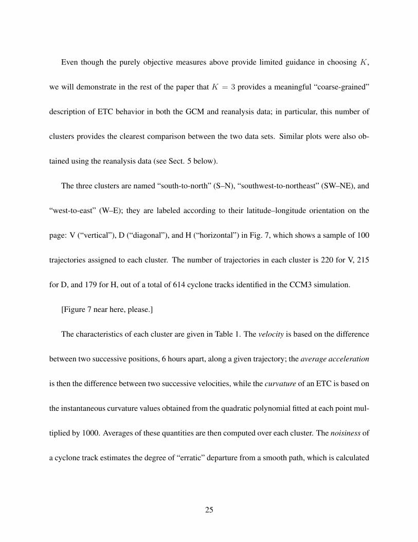
Even though the purely objective measures above provide limited guidance in choosing K,

we will demonstrate in the rest of the paper that K = 3 provides a meaningful “coarse-grained”

description of ETC behavior in both the GCM and reanalysis data; in particular, this number of

clusters provides the clearest comparison between the two data sets. Similar plots were also ob-

tained using the reanalysis data (see Sect. 5 below).

The three clusters are named “south-to-north” (S–N), “southwest-to-northeast” (SW–NE), and

“west-to-east” (W–E); they are labeled according to their latitude–longitude orientation on the

page: V (“vertical”), D (“diagonal”), and H (“horizontal”) in Fig. 7, which shows a sample of 100

trajectories assigned to each cluster. The number of trajectories in each cluster is 220 for V, 215

for D, and 179 for H, out of a total of 614 cyclone tracks identified in the CCM3 simulation.


The characteristics of each cluster are given in Table 1. The velocity is based on the difference

between two successive positions, 6 hours apart, along a given trajectory; the average acceleration

is then the difference between two successive velocities, while the curvature of an ETC is based on

the instantaneous curvature values obtained from the quadratic polynomial fitted at each point mul-

tiplied by 1000. Averages of these quantities are then computed over each cluster. The noisiness of

a cyclone track estimates the degree of “erratic” departure from a smooth path, which is calculated

25

by the standard deviation of instantaneous curvature along the trajectory (also multiplied by 1000).

[Table 1 near here, please.]

The V-cluster consists of relatively short, south-to-north oriented cyclones with large curvature

and noisiness. The cyclones in this cluster are fairly slow with many exhibiting relatively stationary

behavior. The D-cluster consists of a large group of diagonally oriented cyclones that generally

cross the Atlantic travelling from south-west to north-east. These cyclones have the largest average

velocity (59 km/h), intensity (−40 mb), duration (4.1 days), and the smallest noisiness (7.8), as

compared to those in the other two clusters. The H-cluster consists of cyclones that move west to

east, across the western coastlines of Europe. These cyclones are the least intense on average (−34

mb) overall, but have the largest acceleration values (19 km/h2) and curvature (15); a large part of

the curvature can be attributed to erratic behavior, as reflected by their large noisiness of 23.

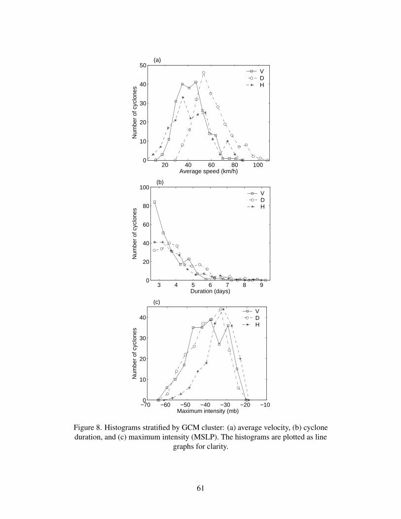
Figure 8 shows histograms of average speed, duration and maximum intensity, stratified by

cluster. Cluster D contains the fastest cyclones in the overall set, with several having average

speeds greater than 80 km/h. Cluster V contains the largest number of short-duration tracks, lasting

3 days or less, and only 6% of the cyclones in cluster V last longer than 5 days, as opposed to 11%

and 18% for clusters H and D, respectively.


26

5. Clustering of cyclones in reanalysis data

In this section we apply our new clustering methodology to reanalyzed cyclone trajectories over

the 44 extended winter seasons. These were tracked in the same manner as the GCM trajectories,

using the same region of 30◦N–80◦N and 80◦W–30◦E as in the GCM analysis; the resulting set

contains 1,915 ETC trajectories. This number is about 3 times larger than the number found in the

GCM data, consistent with the reanalysis data covering about 3 times as many seasons (44 versus

15). Cyclones are active on approximately 75% of the days in the 44-winter data set. Summary

histograms (not shown) of average velocity and maximum intensity are quite similar to those in

Fig. 2 for the GCM data.

We again selected K = 3 clusters for analysis, for ease of comparison with the GCM case.

Plots of log-likelihood and SSE scores (not shown) exhibit similar features to those in Fig. 6 for

the GCM case. There is thus no clear evidence that the appropriate value of K should be any

different, while selecting a common value of K = 3 in both analyses allows for a straightforward

comparison of ETC behavior in the two datasets. This choice was found in Sect. 6 to yield clusters

related to distinct physical phenomena, including the North Atlantic Oscillation (NAO).

The trajectories were first referred to their initial positions, as for the GCM data, but not other-

wise normalized. Figure 9 shows the tracks from each of the three clusters.

27


As in the GCM data set (Fig. 7), the clusters show predominantly vertical (V), diagonal (D),

and horizontal (H) track orientations. The three reanalysis clusters are almost equally populated,

with 680, 604 and 631 trajectories, respectively. The V-cluster has meridional, recurving tracks,

as in CCM3, but is much more heavily concentrated over the western North Atlantic than in the

GCM; it contains the largest number of members. The reanalysis D-cluster also forms a much

narrower diagonal, SW–NE swath of tracks across the Atlantic. Indeed, the GCM’s cyclones are

generally too zonal in their spatial distribution, extending excessively into Europe. The H-cluster

has predominantly eastward oriented tracks but its track distribution is more erratic than in the

GCM.

Compared to the three clusters of Blender et al. (1997, Fig. 3 there), who used a higher-

resolution data set, based on operational analyses of the European Centre for Medium-Range

Weather Forecasts (ECMWF) for 1990–94, our results do not include the “stationary” cyclones

over Greenland and the Mediterranean. Our D-cluster can be equated with the “northeastward”

cluster of these authors, and our H-cluster with their “zonal” one. The largest difference between

the results of Blender and colleagues and those reported here is our heavily populated V-cluster,

with most trajectories close to the coastline of North America.

28


Figure 10 shows histograms of average speed, duration and maximum intensity for the reanal-

ysis trajectories, stratified by cluster, with summary statistics given in Table 2; these display items

are analogous to Fig. 8 and Table 1 for the GCM trajectories. The overall statistical results for the

reanalysis are generally quite consistent with the GCM case (Table 2 vs. Table 1), while some dis-

crepancies appear in the detailed distribution of the ETC tracks (Fig. 10 vs. Fig. 8). The D-cluster

again contains markedly faster moving cyclones (mean velocity of 63 km/h), with the H-cluster

containing the slowest (mean of 38 km/h). The durations are more similarly distributed between

the clusters than in the GCM. The reanalysis H-cluster contains less intense cyclones, qualitatively

similar to the GCM. The reanalysis accelerations are slightly larger in all three cases, and lifetimes

are slightly shorter and differ little between the reanalysis clusters (3.5–3.6 days). In addition, the

reanalysis data set shows relatively fewer D-cluster cyclones, but relatively more D and H tracks

of short duration.

The largest differences between reanalysis and GCM-simulated cyclones are in the curvature

and smoothness of the tracks. The reanalysis cyclones exhibit much smaller curvature and noisi-

ness, across all three clusters. Our results thus indicate that the data assimilation scheme used in

the NCEP-NCAR reanalysis produces fairly smooth ETC trajectories. As in the GCM case, the

29

D-cluster cyclones in the reanalysis tend to have tracks that are straighter and less noisy.

6. Meteorological Composites

Storm-track activity associated with ETCs is typically examined in terms of Eulerian eddy statistics

(e.g., Blackmon et al. 1977; Hurrell et al. 2003), so that it is of interest to compare our Lagrangian

track-based clusters with composites of sub-weekly variance for each cluster. A simple composit-

ing approach follows naturally from the discrete nature of the clustering, which can be contrasted

with the regression approach of Mailier et al. (2006). To construct the composites, a day is as-

signed to a cluster if a cyclone from that cluster is active on that day. If no cyclones are active, the

day is assigned to a fourth, “quiescent” regime. For days with overlap, the regime corresponding

to the cluster with the largest number of active cyclones on that day is chosen. In the case of a tie

between two or more active clusters, the regime which was most recently selected corresponding

to one of the “tied” clusters is chosen; this criterion can be thought of as a type of “inertial bias”.

In the GCM (reanalysis) data, overlap occurs on 15.5% (18.4%) of days.

Composites of anomalous storm-track activity are plotted in Fig. 12 for each cluster, as anoma-

lies in the high-pass filtered MSLP variance; these anomalies are defined with respect to the cli-

matological averages of high-pass variance displayed in Fig. 11. A 7-point high-pass filter with a

30

6.4-day cut-off was used to isolate the ETC variability (Trenberth 1986). The climatological storm

tracks exhibit broadly similar geographical distributions in the reanalysis and GCM MSLP fields

(Figs. 11a,b), with maxima near Newfoundland and Iceland.

[Figure 11 and 12 near here, please.]

The composites of anomalous variance tend to be consistent with the geographical track dis-

tributions of the respective clusters in Figs. 7 and 9. They show some broad similarities between

the two data sets, but with some important differences. In general, the reanalysis composites are

much more spatially coherent, which is consistent with the larger degree of geographical localiza-

tion seen in the corresponding trajectory clusters. In both cases, the “Quiescent” cluster, which

comprises days when no cyclones are active, shows decreased variance over much of the North At-

lantic. The H-cluster also shows a decreased variance over most of the North Atlantic, with slight

enhancement of variance off the coasts of western Europe. The V and D clusters differ the most

between reanalysis and GCM, with the former showing very marked increases in cyclone activity

in the regions expected from Fig. 9. The GCM’s V and D clusters show enhanced variance near

60◦N, consistent with Fig. 7. In summary, while the clustering is based soley on trajectory shape,

the resulting clusters exhibit distictively differing geographical distributions of high-pass MSLP

variance, and this is especially clear in the reanalysis data.

31

One of the motivations for clustering cyclone trajectories is to relate differing cyclone types

to the larger-scale background flow. To this end, we have low-pass filtered 700-hPa geopotential

heights in the reanalysis data, with a 10-day cut-off, and composited the resulting fields for each

cluster. The low frequencies are selected so as to focus on the component of the circulation that

is not directly associated with the cyclones themselves. Maps of the four composites, based on

departures from the grand mean of the 44 winters, are plotted in Fig. 13. All four composites are

characterized by geopotential height anomalies that closely mirror the distributions of ETC tracks

and sub-weekly MSLP variance. The quiescent composite shows a ridge over the climatological

position of the storm track, consistent with reduced cyclone activity, and a weak trough west of

Greenland. The V-cluster is accompanied by a dipole, with a trough centered over Nova Scotia,

and a ridge centered over Iceland. The trough coincides with anomalously high ETC activity.


The D-cluster and H-cluster are accompanied by opposite phases of the NAO (e.g., Hurrell

et al. 2003), with north–south dipoles in geopotential height over the North Atlantic. The D-

cluster corresponds to the positive phase of the NAO, with a trough over Greenland and a ridge to

the south. In this phase, the NAO anomaly amplifies the climatological pressure gradients, leading

to an intensified storm track over the North Atlantic and steering cyclones to the northeast. In

32

the NAO’s negative phase, the climatological gradients are weakened, so that cyclones tend to be

weaker and track more zonally. Our results are consistent with the NAO index regressed onto

root-mean-square transient geopotential height in the 2–8-day band (Hurrell et al. 2003, Fig. 15),

which closely resembles our MSLP sub-weekly variance composites in Figs. 12g and h.

The most-populated cluster in both the reanalysis and the GCM data is the V-cluster; it is asso-

ciated with a large-scale wave pattern that is less familiar from studies of low-frequency variability

than the NAO. This pattern is indeed more transitory than those associated with the D and H clus-

ters, with a larger number of run-lengths shorter than 5 days (not shown). It shares certain features

with the Reverse W3 (RW3) wave train of Mo and Ghil (1988), the eastern Atlantic ridge (AR) of

Vautard (1990), and ATL regime A2 of Kimoto and Ghil (1993). The differences consist mainly

in a zonal shift of the main features and might be due to differences in the domain of analysis and

data set, even more so than to the difference in the compositing. Vautard (1990) notes, in fact, that

the storm track is both shortened and displaced northward for his AR regime.

7. Summary and concluding remarks

Curve-based mixture models were used to perform probabilistic clustering of wintertime North At-

lantic extratropical cyclone (ETC) trajectories in latitude–longitude space. In contrast to previous

33

clustering methods, trajectories have varying durations and the clustering is performed directly in

“trajectory-space” rather than in a fixed-dimensional vector space. Quadratic polynomials were

found to provide the best fits among the regression models we considered (Fig. 4).

An identification and tracking procedure using mean sea level pressure (MSLP) fields was de-

veloped and applied both to an NCAR CCM3 simulation and the NCEP-NCAR reanalysis, over

the North Atlantic. The resulting cyclone trajectories (e.g., Fig. 1) were used as input to the clus-

tering algorithm. The objective performance measures of log-likelihood and the sum of squared

errors (Fig. 6) suggested that K = 3 is a reasonable choice for the number of clusters, in both

the GCM data and the reanalysis, resulting both cases in groups of tracks oriented predominantly

south-to-north (“V”), southwest-to-northeast (“D”), and west-to-east (“H”) respectively (Figs. 7

and 9). These three categories of tracks were found to share several attributes in both the GCM

and reanalysis data (Figs. 8 and 9; Tables 1 and 2). The V-cluster consists of relatively short,

slow-moving cyclones with S–N tracks, and intermediate curvature and noisiness. The D-cluster

cyclones have the largest average velocity, intensity, and duration; their tracks are the straightest

and smoothest of all cyclones. The H-cluster cyclones are relatively slow-moving and are the least

intense on average, but have relatively large acceleration values, and the largest values of curvature

and noisiness in both data sets.

34

The main distinction between the GCM and reanalysis cyclones was found to be in their geo-

graphic distribution, with the reanalysis cyclones being much more geographically localized: the

V-cluster cyclones over the eastern seaboard of North America, the D-cyclones in a narrower cross-

Atlantic swath, and the H-cluster more confined to the Atlantic and northwest Europe (Figs. 7 and

9). Composite maps of sub-weekly “storm track” MSLP variance anomalies were found to be quite

consistent with the track distributions, again with the maps being much more spatially coherent in

the reanalysis case (Fig. 12).

The clustering was performed solely by trajectory shape. Additional experiments (not shown)

indicate that including initial position in the characterization of each ETC yields clusters with

clearly defined geographical centers of gravity , but that the associated cluster composites of geopo-

tential height are less amenable to physical interpretation.

Using K-mean analysis of 3-day-long tracks derived from 5 winters of higher-resolution ECMWF

analysis, Blender et al. (1997) also obtained a total of 3 clusters. Of these, a cluster of near-

stationary cyclones, concentrated over the Mediterranean and near Greenland, largely absent from

our analysis; these cyclones are probably missed in our lower-resolution data set. Of these authors’

two other clusters, the north-eastward one resembles our D-cluster, and their zonal cluster is quite

similar to our H-cluster. Our heavily populated V-cluster, with most trajectories close to the coast-

35

line of North America in the reanalysis data, differs from the results of Blender and colleagues.

The D and H clusters in the reanalysis were found to be closely related to the opposite phases

of the well-known NAO teleconnection pattern (Fig. 13c,d). The positive phase of the NAO is

associated with diagonally oriented tracks with cyclones that are typically faster, more intense, of

longer duration, and with the straightest and smoothest tracks. This contrasts with the horizontally

oriented tracks that characterize the NAO’s negative phase, which are typically weaker, moving

more slowly, and fairly erratic. This association with the phases of the NAO arises out of our

clustering that is based purely on trajectory shape. We conclude that this statistical association

does have a physical explanation in terms of the dynamical features of the opposite NAO phases.

The most highly populated V-cluster was found to be associated in the reanalysis with a trough

over the western and a ridge over the eastern North Atlantic (Fig. 13b). This large-scale feature has

been identified by various names in different studies: RW3 in Mo and Ghil (1988), AR in Vautard

(1990), and A2 in Kimoto and Ghil (1993). The ridge blocks the eastward propagation of the

ETCs, while the trough favors their northward evolution. To summarize, the ease of comparison

between GCM clusters and those in the reanalysis, as well as the physical interpretation of the

latter, support the choice of three clusters as a good coarse-grained description of ETC behavior

over the North Atlantic. We note, furthermore, that these three clusters also agree with three of

36

the four regimes obtained by Yiou and Nogaj (2004) in classifying extremes of precipitation and

temperature over a similar area.

Having demonstrated that, in reanalysis data, the cyclone-track clusters are associated with

well-defined anomalies in sub-weekly storm track variance and well-known low-frequency tele-

connection patterns, we argue that further analysis of ETC track behavior from the Lagrangian

perspective used in this paper could enable a more fundamental interpretation of these features.

Unlike in the case of the reanalysis data, meteorological composites constructed from the 15-

winter GCM simulation did not provide conclusive evidence for associations between ETC track

behavior and large-scale circulation patterns in the simulation. The methodology clearly high-

lights the limitations of the GCM, while the GCM is shown nonetheless to capture cyclone tracks

of quite realistic orientation, as well as several associated features of cyclone intensity, speed and

lifetimes. Lagrangian diagnostics could thus provide important tools in assessing GCM perfor-

mance for studies of climate variability and change. The method has, therefore, also been applied

to clustering of tropical cyclone tracks over the western tropical North Pacific (Camargo et al.

2006a,b). The software developed and used in this study is freely available to other investigators

from http://www.datalab.uci.edu/resources/CCT/. We hope that the methodology will prove useful

in further studies of ETC behavior in models and observations.

37

Acknowledgments: We wish to thank Kevin Hodges for helpful discussions, and Jim Boyle and

Peter Glecker for help in obtaining the NCAR CCM3 data. We are grateful to Kevin Hodges and

two anonymous referees for their constructive reviews which substantially improved the paper. The

NCEP-NCAR Reanalysis data were provided by the NOAA CIRES Climate Diagnostics Center,

Boulder, Colorado, from their Web site available online at http://www.cdc.noaa.gov. This work

was supported in part by a Department of Energy grant DE-FG02-02ER63413 (MG and AWR), by

NOAA through a block grant to the International Research Institute for Climate and Society (SJC

and AWR), and by the National Science Foundation under grants No. SCI-0225642, IIS-0431085,

and ATM-0530926 (SJG and PS).

Appendix A

Expectation Maximization Algorithm

The EM algorithm is an iterative maximum likelihood (ML) procedure that provides a general and

efficient framework for parameter estimation. At a base level, EM is an approximate root-finding

procedure used to seek the root of the likelihood equation by iteratively searching for a set of

parameters that maximize the probability of the observed data. EM is primarily used for finding

38

ML parameter estimates in missing- or hidden-data problems. Parameter estimation in hidden-data

problems is difficult because the likelihood equation takes on a complex form, often involving an

integral or a sum over the hidden data itself.

For example, Eqn. (5) in Sect. 3.c gives the likelihood of φ given both Z and T (repeated here):

L(φ|Z, T ) = p(Z|T , φ) =n∏i

K∑k

αk fk(zi|Tiβk, Σk). (A1)

Notice that the hidden data in this case are the unknown cluster memberships which must be

summed-out of the likelihood to arrive at L(φ|Z, T ). It is understood in hidden-data problems that

this operation cannot be easily carried out. The EM algorithm is an iterative two-step procedure

used to circumvent this integration (or sum) by (1) indirectly estimating values for the unobserved

data, and (2) finding the ML parameter estimates that correspond to the now completely observed

data. The new ML estimates from step (2) are then used to re-estimate the hidden data in step

(1), and these iterations are continued until some stopping criterion is reached (typically this in-

volves stopping when the change in log-likelihood falls below a particular threshold, and thus the

iterations have stabilized).

In the first step, the E-step, we estimate the hidden cluster memberships by forming the ratio

39

of the likelihood of trajectory i under cluster k, to the sum-total likelihood of trajectory i under all

clusters:

wik =αkfk(zi|Tiβk, Σk)∑Kj αjfj(zi|Tiβj, Σj)

(A2)

These wik give the probabilities that the i-th trajectory was generated from cluster k. They rep-

resent a posterior expectation for the value of the actual binary cluster memberships (i.e., the i-th

trajectory was either generated by the k-th cluster or it was not).

In the second step, the M-step, the expected cluster memberships from the E-step are used to

form the weighted log-likelihood function:

L(φ|Z, T ) =n∑i

K∑k

wik log αk fk(zi|Tiβk, Σk). (A3)

The membership probabilities weight the contribution that the k-th density component adds to the

overall likelihood. In the case where the wik are binary, and thus cluster membership is perfectly

known, this reduces to the usual fully-observed log-likelihood. This weighted log-likelihood is

then maximized with respect to the parameter set φ.

For the sake of completeness, we give each of the re-estimation equations below. Let wik =

wikIni, where Ini

is an ni-vector of ones, and let Wk = diag(w′1k, . . . ,w

′nk) be an N×N diagonal

40

matrix. Then, in the M-step we use Wk to calculate the mixture parameters

βk = (T′WkT)−1T′WkZ, (A4)

Σk =(Z−Tβk)

′Wk(Z−Tβk)∑ni wik

, (A5)

and the mixture weights

αk =1

n

n∑i

wik (A6)

for k = 1, . . . , K. These update equations are equivalent to the well-known weighted least-squares

solution in regression (Draper and Smith 1981). The diagonal elements of Wk represent the

weights to be applied to Z and T during the weighted regression.

Because most of the difficult work is carried out in estimating the cluster memberships, the

maximization carried out in the M-step is straightforward. This is a common attribute of the EM

algorithm. Dempster et al. (1977b) showed that under fairly general conditions, the likelihood will

never decrease during the E- and M-step iterations. Due to the presence of local maxima on the

likelihood surface, the solution is not guaranteed to correspond to a global maximum. However,

41

we can increase the chances of finding the global maximum by running the EM algorithm multiple

times from different starting points in parameter space and selecting the parameters that result in

the highest overall likelihood.

42

References

Anderson D, Hodges KI, Hoskins BJ (2003) Sensitivity of Feature-Based Analysis Methods of

Storm Tracks to the Form of Background Field. Mon Wea Rev 131(3):565–573

Bernardo JM, Smith AFM (1994) Bayesian Theory, Wiley, New York

Blackmon ML, Wallace JM, Lau NC, Mullen SL (1977) An Observational Study of the Northern

Hemisphere Wintertime Circulation. J Atmos Sci 34:1040–1053

Blender R, Fraedrich K, Lunkeit F (1997) Identification of cyclone-track regimes in the North

Atlantic. Quart J Royal Meteor Soc 123:727–741

Camargo SJ, Robertson AW, Gaffney SJ, Smyth P (2006a) Cluster Analysis of Typhoon Tracks.

Part I: General Properties. J Climate in press

Camargo SJ, Robertson AW, Gaffney SJ, Smyth P (2006b) Cluster Analysis of Typhoon Tracks.

Part II: Large-Scale Circulation and ENSO. J Climate in press

Dempster AP, Laird NM, Rubin DB (1977a) Maximum likelihood from incomplete data via the

EM algorithm. J Royal Stat Soc B 39:1–38

43

Dempster AP, Laird NM, Rubin DB (1977b) Maximum likelihood from incomplete data via the

EM algorithm. J Royal Stat Soc B 39:1–38

DeSarbo WS, Cron WL (1988) A maximum likelihood methodology for clusterwise linear regres-

sion. J Classification 5(1):249–282

Draper NR, Smith H (1981) Applied Regression Analysis, John Wiley and Sons, New York, NY,

2nd ed.

Elsner JB (2003) Tracking hurricanes. Bull Amer Meteor Soc 84(3):353–356

Elsner JB, b Liu K, Kocher B (2000) Spatial variations in major US hurricane activity: Statistics

and a physical mechanism. J Climate 13:2293–2305

Fraley C, Raftery AE (1998) How many clusters? Which clustering methods? Answers via model-

based cluster analysis. The Computer Journal 41(8):578–588

Fraley C, Raftery AE (2002) Model-based clustering, discriminant analysis, and density estima-

tion. J Amer Stat Assoc 97(458):611–631

Fyfe JC (2003) Extratropical Southern Hemisphere Cyclones: Harbingers of Climate Change. J

Climate 16:2802–2805

44

Gaffney S, Smyth P (1999) Trajectory Clustering with Mixtures of Regression Models, in S Chaud-

huri, D Madigan, (eds.) Proc. Fifth ACM SIGKDD Internat. Conf. on Knowledge Discovery and

Data Mining, pp. 63–72, ACM Press, N.Y.

Gaffney SJ (2004) Probabilistic Curve-Aligned Clustering and Prediction with Regression Mixture

Models, Ph.D. Dissertation, Department of Computer Science, University of California, Irvine

Gaffney SJ, Smyth P (2003) Curve Clustering with Random Effects Regression Mixtures, in

CM Bishop, BJ Frey, (eds.) Proc. 9th Internat. Workshop on Artificial Intelligence and Statistics,

Key West, FL

Gneiting T, Raftery AE (2004) Strictly proper scoring rules, prediction, and estimation, Tech. Rep.

463, Department of Statistics, University of Washington

Hack JJ, Kiehl JT, J. W. H (1998) The Hydrologic and Thermodynamic Characteristics of the

NCAR CCM3. J Climate 11:1179–1206

Hannachi A, O’Neill A (2001) Atmospheric multiple equilibria and non-Gaussian behaviour in

model simulations. Quart J Royal Meteor Soc 127(573):939–958

Hartigan JA, Wong MA (1978) Algorithm AS 136: A K-means clustering algorithm. Appl Stat

28:100–108

45

Hodges KI (1994) A general method for tracking analysis and its applications to meteorological

data. Mon Wea Rev 122(11):2573–2586

Hodges KI (1995) Feature tracking on the unit sphere. Mon Wea Rev 123(12):3458–3465

Hodges KI (1998) Feature-point detection using distance transforms: Application to tracking trop-

ical convective complexes. Mon Wea Rev 126(3):785–795

Hoskins BJ, Hodges KI (2002) New Perspectives on the Northern Hemisphere Winter Storm

Tracks. J Atmos Sci 59(6):1041–1061

Hurrell JW, Kushnir Y, Ottersen G, Visbeck M (2003) An overview of the North Atlantic Oscilla-

tion. Geophys Monogr 134:2217–2231

Kalnay E, Kanamitsu M, Kistler R, Collins W, Deaven D, Gandin L, Iredell M, Saha S, White G,

Woollen J, Zhu Y, Chelliah M, Ebisuzaki W, Higgins W, Janowiak J, Mo K, Ropelewski C, Wang

J, Leetmaa A, Reynolds R, Jenne R, Joseph D (1996) The NCEP/NCAR 40-year reanalysis

project. Bull Amer Meteor Soc 77:437–441

Kimoto M, Ghil M (1993) Multiple Flow Regimes in the Northern Hemisphere Winter. Part II:

Sectorial Regimes and Preferred Transitions. J Atmos Sci 16:2645–2673

46

Konig W, Sausen R, Sielman F (1993) Objective identification of cyclones in GCM simulations. J

Climate 6(12):2217–2231

Lau NC (1988) Variability of the Observed Midlatitude Storm Tracks in Relation to Low-

Frequency Changes in the Circulation Pattern. J Atmos Sci 45:2718–2743

Le Treut H, Kalnay E (1990) Comparison of observed and simulated cyclone frequency distribution

as determined by an objective method. Atmosfera 3:57–71

Lenk PJ, DeSarbo WS (2000) Bayesian inference for finite mixtures of generalized linear models

with random effects. Psychometrika 65(1):93–119

Lwin T, Martin PJ (1989) Probits of mixtures. Biometrics 45:721–732

Mailier PJ, Stephenson DB, Ferro CAT, Hodges KJ (2006) Serial Clustering of Extratropical Cy-

clones. Monthly Weather Review 134:2224–2240

McLachlan G, Krishnan T (1997) The EM Algorithm and Extensions, John Wiley and Sons, New

York, NY

McLachlan GJ, Basford KE (1988) Mixture Models: Inference and Applications to Clustering,

Marcel Dekker, New York

47

McLachlan GJ, Peel D (2000) Finite Mixture Models, John Wiley & Sons, New York

Mesrobian E, Muntz R, Shek E, Mechoso CR, Farrara J, Spahr J, Stolorz P (1995) Real Time Data

Mining, Management, and Visualization of GCM Output. Supercomputing 94 IEEEComputer-

Society pp. 81–87

Mo K, Ghil M (1988) Cluster analysis of multiple planetary flow regimes. J Geophys Res

93D:10927–10952

MunichRe (2002) Winter storms in Europe (II). Analysis of 1999 losses and loss potentials,

Tech. Rep. Rep. 302-03109, 72pp, [Available from Munchner Ruckversicherungs-Gesellschaft,

Koniginstr. 107, 80802 Munchen, Germany.]

Murray RJ, Simmonds I (1991) A numerical scheme for tracking cyclone centres from digital data

Part I: Development and operation of the scheme. Aust Meteor Mag 39:155–166

Preisendorfer RW (1988) Principal Component Analysis in Meteorology and Oceanography, Else-

vier, Amsterdam

Ramsay JO, Silverman BW (1997) Functional Data Analysis, Springer-Verlag, New York, NY

Ramsay JO, Silverman BW (2002) Applied Functional Data Analysis: Methods and Case Studies,

Springer-Verlag, New York, NY

48

Robertson AW, Metz W (1990) Transient-Eddy Feedbacks Derived from Linear Theory and Ob-

servations. J Atmos Sci 47:2743–2764

Saunders MA (1999) Earth’s future climate. Phil Trans Royal Soc Lond A 357:3459–3480

Simmons AJ, Hoskins BJ (1978) The Life Cycles of Some Nonlinear Baroclinic Waves. J Atmos

Sci 35(3):414–432

Smyth P (2000) Model selection for probabilistic clustering using cross-validated likelihood.

Statistics and Computing 10(1):63–72

Smyth P, Ide K, Ghil M (1999) Multiple regimes in northern hemisphere height fields via mixture

model clustering. J Atmos Sci 56(21):3704–3723

Terry J, Atlas R (1996) Objective Cyclone Tracking and its Applications to ERS-1 Scatterometer

Forecast Impact Studies, in 15th Conf. Weather Analysis & Forecasting, American Meteorolog-

ical Society, Norfolk, VA.

Trenberth KE (1986) An Assessment of the Impact of Transient Eddies on the Zonal Flow during a

Blocking Episode Using Localized Eliassen-Palm Flux Diagnostics. J Atmos Sci 43:2070–2087

Vautard R (1990) Multiple Weather Regimes over the North Atlantic: Analysis of Precursors and

Successors. Mon Wea Rev 45:2845–2867

49

von Storch H, Zwiers FW (1999) Statistical Analysis in Climate Research, Cambridge University

Press, Cambridge, MA

Vrac M, Chedin A, Diday E (2005) Clustering a Global Field of Atmospheric Profiles by Mixture

Decomposition of Copulas. Journal of Atmospheric and Oceanic Technology 22(10):1445–1459

Wang K, Gasser T (1997) Alignment of curves by dynamic time warping. Annal Stat 25:1251–

1276

Yiou P, Nogaj M (2004) Extreme climatic events and weather regimes over the North Atlantic:

When and where? Geophys Res Lett 31:L07202, doi:10.1029/2003GL019119

50

List of Figures

1 Random sample of 200 CCM3 cyclone trajectories tracked over the North Atlantic

domain of interest. The circles indicate initial starting position. . . . . . . . . . . . 54

2 Summary histograms for GCM cyclone data set: (a) cyclone duration, (b) average

velocity, and (c) maximum intensity (MSLP). . . . . . . . . . . . . . . . . . . . . 55

3 Performance of the EM algorithm as applied to synthetic trajectories, generated by

a polynomial-regression mixture model: (a) set of synthetic trajectories presented

to the algorithm (the x-es, circles, and squares denote the 3 generating models,

and the different line-types show the 4 different sample curves for each); (b) initial

random starting curves (solid) for the three clusters, with all data points shown as

circles; (c) cluster locations (solid) after EM convergence (iteration 4), as well as

the locations of the true data-generating trajectories (dotted). . . . . . . . . . . . . 56

4 Quadratic polynomial regression models (dotted) fitted to a random sample of three

GCM cyclone trajectories (solid) in the latitude–time plane. . . . . . . . . . . . . . 57

5 GCM cyclone cluster models when K = 2, 3, 4, 5, and 6. . . . . . . . . . . . . . . 58

51

6 Objective test scores of model fit as a function of K for GCM cyclone cluster

models. (a) Cross-validated log-likelihood; and (b) cross-validated sum of squared

errors (SSE). See text for details. . . . . . . . . . . . . . . . . . . . . . . . . . . . 59

7 Clusters derived from GCM data: (V) south-to-north, (D) southwest-to-northeast,

and (H) west-to-east oriented tracks. For each cluster only 100 random tracks are

shown for clarity. . . . . . . . . . . . . . . . . . . . . . . . . . . . . . . . . . . . 60

8 Histograms stratified by GCM cluster: (a) average velocity, (b) cyclone duration,

and (c) maximum intensity (MSLP). The histograms are plotted as line graphs for

clarity. . . . . . . . . . . . . . . . . . . . . . . . . . . . . . . . . . . . . . . . . . 61

9 Clusters derived from reanalysis data: (V) south-to-north, (D) southwest-to-northeast,

and (H) west-to-east. For each cluster 100 random tracks are shown for clarity. . . 62

10 Histograms of reanalysis trajectories stratified by cluster: (a) average velocity, (b)

cyclone duration, and (c) maximum intensity (MSLP). The histograms are plotted

as line graphs for clarity. . . . . . . . . . . . . . . . . . . . . . . . . . . . . . . . 63

11 Mean climatologies of high-pass filtered MSLP variance for the (a) GCM and (b)

reanalysis data sets. Contour interval: 5 hPa2. . . . . . . . . . . . . . . . . . . . . 64

52

12 Composites of high-pass filtered MSLP variance anomalies over the days assigned

to each cluster, for the GCM (a–d) and reanalysis (e–h) data sets. In each case the

respective climatological time average of variance has been subtracted. Positive

contours are solid and negative ones are dashed; contour interval: 1 hPa2. . . . . . 65

13 Composites of low-pass filtered 700-hPa geopotential height anomalies for the

days assigned into each reanalysis cluster. In each case the 44-winter time average

has been subtracted. The shaded regions are significant at the 99% level according

to a two-sided Student t-test with 120 degrees of freedom; this number is smaller

than the number of days in each composite divided by 10. Contour interval: 5 m. . 66

53

60° N

45° N

30° N

30° E 0° 30° W 60° W

75° N

Figure 1. Random sample of 200 CCM3 cyclone trajectories tracked over the North Atlanticdomain of interest. The circles indicate initial starting position.

54

3 4 5 6 7 8 90

20

40

60

80

100

120

140

Duration (days)

Num

ber

of c

yclo

nes

(a)

0 20 40 60 80 100 1200

20

40

60

80

Average velocity (km/h)

Num

ber

of c

yclo

nes

(b)

−70 −60 −50 −40 −30 −200

10

20

30

40

50

60

Maximum intensity (mb)

Num

ber

of c

yclo

nes

(c)

Figure 2. Summary histograms for GCM cyclone data set: (a) cyclone duration,(b) average velocity, and (c) maximum intensity (MSLP).

55

0

100

200

300

400

X-axis

(a)

Fun

ctio

n v

alu

e

0 10 20 30 40

0

100

200

300

400

X-axis

(b)

Func

tion

valu

e

0 10 20 30 40

0

100

200

300

400(c)

Func

tion

valu

e

0 10 20 30 40X-axis

Figure 3. Performance of the EM algorithm as applied to synthetic trajectories, generated by apolynomial-regression mixture model: (a) set of synthetic trajectories presented to the algorithm(the x-es, circles, and squares denote the 3 generating models, and the different line-types show

the 4 different sample curves for each); (b) initial random starting curves (solid) for the threeclusters, with all data points shown as circles; (c) cluster locations (solid) after EM convergence

(iteration 4), as well as the locations of the true data-generating trajectories (dotted).56

0 5 10 15

45

50

55

60

65

Time

Latit

ude

Figure 4. Quadratic polynomial regression models (dotted) fitted to a random sample of threeGCM cyclone trajectories (solid) in the latitude–time (days) plane.

57

0 10 20 30 40

0

5

10

15

20

25

Relative longitude

Rel

ativ

e la

titud

e

K=2

10 20 30 40

0

5

10

15

20

25

Relative longitude

Rel

ativ

e la

titud

e

K=3

10 20 30 40

0

5

10

15

20

25

Relative longitude

Rel

ativ

e la

titud

e

K=4

10 20 30 40

0

5

10

15

20

25

Relative longitude

Rel

ativ

e la

titud

e

K=5

0 10 20 30 40 50

0

10

20

30

Relative longitude

Rel

ativ

e la

titud

e

K=6

Figure 5. GCM cyclone cluster models when K = 2, 3, 4, 5, and 6.

58

! " # $ % & ' ( ) !* !! !" !# !$ !%!#+(

!#+'

!#+&

!#+%

!#+$

!#+#

!#+"

!#+!

!#

!"+)

!"+(

t-./0123!456-457228

9:;<-=02>0?2;@2A-A/.1 2 3 4 5 6 7 8 9 10 11 12 13 14 15

50

100

150

200

250

300

350

400

test S

SE

Number of components

b)a)

Figure 6. Objective test scores of model fit as a function of K for GCM cyclone cluster models.(a) Cross-validated log-likelihood; and (b) cross-validated sum of squared errors (SSE). See text

for details.

59

(V) 60° W 30° W 0° 30° E

30° N

45° N

60° N

75° N

(D) 60° W 30° W 0° 30° E

30° N

45° N

60° N

75° N

(H) 60° W 30° W 0° 30° E

30° N

45° N

60° N

75° N

Figure 7. Clusters derived from GCM data: (V) south-to-north, (D) southwest-to-northeast, and(H) west-to-east oriented tracks. For each cluster only 100 random tracks are shown for clarity.

60

20 40 60 80 1000

10

20

30

40

50

Average speed (km/h)

Num

ber

of c

yclo

nes

(a)

VDH

3 4 5 6 7 8 90

20

40

60

80

100

Duration (days)

Num

ber

of c

yclo

nes

(b)

VDH

−70 −60 −50 −40 −30 −20 −100

10

20

30

40


Num

ber

of c

yclo

nes

(c)

VDH

Figure 8. Histograms stratified by GCM cluster: (a) average velocity, (b) cycloneduration, and (c) maximum intensity (MSLP). The histograms are plotted as line

graphs for clarity.

61

(V) 60° W 30° W 0° 30° E

30° N

45° N

60° N

75° N

(D) 60° W 30° W 0° 30° E

30° N

45° N

60° N

75° N

(H) 60° W 30° W 0° 30° E

30° N

45° N

60° N

75° N

Figure 9. Clusters derived from reanalysis data: (V) south-to-north, (D) southwest-to-northeast,and (H) west-to-east. For each cluster 100 random tracks are shown for clarity.

62

20 40 60 80 1000

20

40

60

80

100

120

140

Average speed (km/h)

Num

ber

of c

yclo

nes

(a)

VDH

3 4 5 6 7 8 90

50

100

150

200

250

300

Duration (days)

Num

ber

of c

yclo

nes

(b)

VDH

−80 −70 −60 −50 −40 −30 −20 −100

20

40

60

80

100

120


Num

ber

of c

yclo

nes

(c)

VDH

Figure 10. Histograms of reanalysis trajectories stratified by cluster: (a) averagevelocity, (b) cyclone duration, and (c) maximum intensity (MSLP). The

histograms are plotted as line graphs for clarity.

63

GMT 2006 Jun 4 04:35:37 climo_var

OBS vs GCM High-Pass SLP Variance

20˚

40˚

60˚

80˚

10

10

20

20

20

20

3030

30

304050

a) GCM High-pass Variance

240˚ 270˚ 300˚ 330˚ 0˚ 30˚20˚

40˚

60˚

80˚

10

10

20

20

20

30

30

30

30

30

40

40

b) Obs High-pass Variance

Figure 11. Mean climatologies of high-pass filtered MSLP variance for the (a) GCM and (b)reanalysis data sets. Contour interval: 5 hPa2.

64

2006 Jun 17 08:45:52 psl_HT_varcomps

GCM

20˚N

40˚N

60˚N

80˚N

-4

-4-2

-2

-2 -2

-2

2

2

2

22

4 4

a) Quiescent Cluster (635 days)

20˚N

40˚N

60˚N

80˚N

2

2

2

24

4

6

b) V-Cluster (714 days)

20˚N

40˚N

60˚N

80˚N

-2-2

-2-2

2

2

2

2

2

2

4

4

c) "D-Cluster (799 days)

120˚W 90˚W 60˚W 30˚W 0˚ 330˚W20˚N

40˚N

60˚N

80˚N

-6 -6

-4

-4

-4

-4

-4-4

-2

-2

-2

-2-2

-2

2

d) "H-Cluster (567 days)

2006 Jun 17 08:45:35 ncep_slpHT_K3_2p5d_zero_varcomps_an

Reanalysis

20˚N

40˚N

60˚N

80˚N

-8

-6

-4

-4-2

-2

-2

222

2 4

4

e) Quiescent Cluster (2014 days)

20˚N

40˚N

60˚N

80˚N

-2

-2

2

2

2

4

4

6

68

f) V-Cluster (2333 days)

20˚N

40˚N

60˚N

80˚N-6

-6

-4-4-4

-2

-2

22

2

2

4

44

6

6

6 8

8

101012

g) D-Cluster (1793 days)

120˚W 90˚W 60˚W 30˚W 0˚ 330˚W20˚N

40˚N

60˚N

80˚N

-10

-10

-10

-8

-8

-6

-6

-6

-4

-4

-4 -4

-2-2

-2

-2

2

h) H-Cluster (1824 days)

Figure 12. Composites of high-pass filtered MSLP variance anomalies over the days assigned toeach cluster, for the GCM (a–d) and reanalysis (e–h) data sets. In each case the respective

climatological time average of variance has been subtracted. Positive contours are solid andnegative ones are dashed; contour interval: 1 hPa2.

65

GMT 2005 Apr 5 21:32:08 z700lpan_BW

Z700 LP Anomaly Composites for Cyclone Clusters

a) Quiescent Cluster (2014 days) b) V-Cluster (2333 days)

c) D-Cluster (1793 days) d) H-Cluster (1824 days)

0˚30˚

60˚90˚

120˚

150˚

180˚210˚

240˚270˚

300˚

330˚

10

0˚30˚

60˚90˚

120˚

150˚

180˚210˚

240˚270˚

300˚

330˚

-10

0˚30˚

60˚90˚

120˚

150˚

180˚210˚

240˚270˚

300˚

330˚

-30

-10

10

0˚30˚

60˚90˚

120˚

150˚

180˚210˚

240˚270˚

300˚

330˚

-1030

Figure 13. Composites of low-pass filtered 700-hPa geopotential height anomalies for the daysassigned into each reanalysis cluster. In each case the 44-winter time average has been subtracted.

The shaded regions are significant at the 99% level according to a two-sided Student t-test with120 degrees of freedom; this number is smaller than the number of days in each composite

divided by 10. Contour interval: 5 m.

66

List of Tables

1 Cluster-wide average measures for various GCM cyclone statistics. Both means

(µ) and standard deviations (σ) are given for each cluster. . . . . . . . . . . . . . . 68

2 Cluster-wide average measures for various reanalysis cyclone statistics. Both means

(µ) and standard deviations (σ) are given for each cluster column. . . . . . . . . . 69

67

TABLE 1. Cluster-wide average measures for various GCM cyclone statistics. Both means (µ)and standard deviations (σ) are given for each cluster.

Cluster-specific statistics V D Hµ σ µ σ µ σ

Maximum intensity (mb) -39.9 8.9 -40.0 8.2 -33.8 7.4Average velocity (km/h) 42.5 11.5 59.4 13.8 42.8 15.9Average acceleration (km/h2) 15.4 5.7 16.5 5.6 18.8 7.5Lifetime (days) 3.6 0.10 4.1 1.2 3.8 1.2Curvature 12.1 22.0 4.8 5.2 15.2 17.8Noisiness 19.1 48.4 7.8 13.1 23.5 35.8

68

TABLE 2. Cluster-wide average measures for various reanalysis cyclone statistics. Both means(µ) and standard deviations (σ) are given for each cluster column.

Reanalysis cluster-specific statistics V D Hµ σ µ σ µ σ

Maximum intensity (mb) -39.1 8.5 -39.2 8.1 -35.4 7.8Average velocity (km/h) 43.9 10.5 62.6 12.9 37.8 12.76Average acceleration (km/h2) 18.0 7.1 19.6 6.9 19.5 8.0Lifetime (days) 3.5 0.9 3.6 1.1 3.5 1.2Curvature 2.9 3.1 1.8 1.9 6.2 5.5Noisiness 4.6 6.9 3.2 3.8 8.6 9.6

69

Probabilistic Clustering of Extratropical Cyclones Using...

Documents

Transcript of Probabilistic Clustering of Extratropical Cyclones Using...