Probabilistic Bridge Weigh-in-Motion · Draft 1 Probabilistic Bridge Weigh-in-Motion Eugene J....

Draft

Probabilistic Bridge Weigh-in-Motion

Journal: Canadian Journal of Civil Engineering

Manuscript ID cjce-2017-0508.R1

Manuscript Type: Article

Date Submitted by the Author: 24-Nov-2017

Complete List of Authors: OBrien, Eugene J.; University College Dublin, Civil Engineering Zhang, Longwei; college of civil engineering, ; UCD school of civil, structural and environmental engineering , Zhao, Hua; college of civil engineering, Department of bridge engineering Hajializadeh, Donya; Roughan & O'Donovan,

Is the invited manuscript for consideration in a Special

Issue? : Not Applicable (Regular Submission)

Keyword: BWIM, PWIM, Bridge Load Modelling, Vehicle Loading, vehicle-bridge interaction finite element

https://mc06.manuscriptcentral.com/cjce-pubs

Canadian Journal of Civil Engineering

Draft

1

Probabilistic Bridge Weigh-in-Motion

Eugene J. OBriena,e Longwei Zhangb,e, Hua Zhaoc, Donya Hajializadehd, *

a School of Civil Engineering, University College Dublin, Belfield, Dublin 4, Ireland

b China Minsheng Drawin Technology Group, Changsha, Hunan, China

c Key Laboratory for Wind and Bridge Engineering of Hunan Province, Hunan University, Changsha,

Hunan, China

d Department of Engineering & the Built Environment, Faculty of Science & Technology, Anglia Ruskin

University, Essex, United Kingdom

e These authors contributed equally to this work and should be considered joint first authors

* corresponding author: email, [email protected]

Page 1 of 40



Draft

2

Abstract

Conventional bridge weigh-in-motion (BWIM) uses a bridge influence line to find the axle

weights of passing vehicles that minimize the sum of squares of differences between theoretical

and measured responses. An alternative approach, probabilistic bridge weigh-in-motion (pBWIM),

is proposed here. The pBWIM approach uses a probabilistic influence line and seeks to find the

most probable axle weights, given the measurements. The inferred axle weights are those with the

greatest probability amongst all possible combinations of values. The measurement sensors used

in pBWIM are similar to BWIM, containing free-of-axle detector (FAD) sensors to calculate axle

spacings and vehicle speed and weighing sensors to record deformations of the bridge. The

pBWIM concept is tested here using a numerical model and a bridge in Slovenia. In a simulation,

two hundred randomly generated 2-axle trucks pass over a 6 m long simply supported beam. The

bending moment at mid-span is used to find the axle weights. In the field tests, seventy-seven pre-

weighed trucks traveled over an integral slab bridge and the strain response in the soffit at mid-

span was recorded. Results show that pBWIM has good potential to improve the accuracy of

BWIM.

Page 2 of 40



Draft

3

1. Introduction

As the main imposed loads on a bridge, the weights of vehicles play an important role in

determining its safety (Yu et al. 2016). With increasing vehicle loading and a generally ageing

bridge stock in the developed world, many existing bridges have suffered substantial deterioration

which will shorten their service lives (Lydon et al. 2016). Road authorities sometimes use weigh-

in-motion (WIM) systems to get information about the traffic acting on bridges and to inform

them about the requirements for enforcement of the maximum weight limits (Blab and Jacob

2000). With 56% of bridges assessed every three years in Canada (Canadian Infrastructure 2016),

utilizing accurate weighing systems could result in significant savings.

According to Zhang et al. 2007, WIM was first introduced to Canada in Alberta in 1982 and

its usage has been increasing steadily. There are two categories of WIM system: pavement-based

WIM and bridge WIM (BWIM). Pavement-based WIM systems utilize sensors embedded in the

pavement to measure the instantaneous forces while the tire passes over the sensors (Jacob 1999,

Jacob et al. 2002). BWIM systems, first developed by Moses (1979), use an existing bridge as a

scale to find the weights of vehicles passing overhead. In Moses’ approach, BWIM is made up of

two parts. One part consists of axle detectors monitoring axle numbers, spacings and vehicle

speed. The other part consists of weighing sensors, usually strain transducers, recording the

deformation of the bridge while vehicles cross over.

Both types of WIM system can take measurements directly and calculate axle weights while

vehicles are moving at full highway speed (Richardson et al. 2014). Due to the very short

recording time and vehicle-pavement dynamics, the accuracy of pavement-based WIM systems is

limited by the width of the sensors and the roughness of the road profile (González 2010). In

contrast, BWIM systems use the continuous response of the bridge for the time the vehicle takes

to pass overhead. The response measurement period is much greater than the recording time for

pavement-based WIM systems. This makes BWIM much less sensitive to vehicle dynamics and

Page 3 of 40



Draft

4

gives it the potential for greater accuracy, especially on rough roads. BWIM systems also have

other advantages over pavement-based WIM systems in terms of durability and portability

(OBrien et al. 1999) but there will always be the limitation that a bridge is required at the site of

interest.

Modern commercial BWIM systems are based on Moses’ algorithm and variations of it

(OBrien et al. 2008). To find axle weights, an error function E (Eq. 1), is defined as the sum of

squares of differences between the measured and theoretical responses caused by passing vehicles

(Moses 1979):

2

1

[ ]K

M T

i i

i

E R R=

= −∑ (1)

where i is the scan number; K is the total number of scans; M

iR and T

iR are the measured and

theoretical responses respectively at scan i. In the original Moses’ algorithm, the theoretical

response is taken as the sum of products of axle weights and the corresponding theoretical

influence line ordinates. The theoretical influence line is now known to provide a poor

representation of the real behavior of a bridge, so a modified influence line based on

measurements is applied to improve accuracy. Žnidarič and Baumgartner (1998) adjusted the

support conditions and smoothed the peaks to get an influence line of better consistency with the

real situation. McNulty and OBrien (2003) developed a ‘point-by-point’ graphical method of

manually deriving the influence line. OBrien et al. (2006) improved on this by proposing a

‘matrix’ method of calculating the ‘measured’ influence line ordinates that best fit the response to

a calibration truck of known axle weights. In effect, the error function of Eq. 1 is minimized to

determine the unknown influence ordinates as opposed to the axle weights.

In the United States and Canada there have been several studies in the improvement of the

accuracy of BWIM methods since Moses’ early work. For example Bakht et al. (2006) tested the

accuracy of the reaction force theory developed by Yamada & Ojio (2003) using an instrumented

bridge in Manitoba. Their study shows a high sensitivity of strains to transverse position of the

Page 4 of 40



Draft

5

vehicle on the bridge and hence inaccurate axle weights for trucks in certain transverse positions.

Helmi et al. (2014) conducted a comparative study of three BWIM methods. In two of these the

truck load is represented by an equivalent uniformly distributed load and in the third GVW is

estimated using strain signal area as proposed by Yamada & Ojio (2003). The study found

inconsistency in accuracy in the first method, reduced accuracy with vehicle length in the second

and less than 5% error in GVW in the third. Faraz et al. (2017) reported similar results for these

techniques when identifying sources of error in the fatigue evaluation of South Perimeter Bridge.

The BWIM method developed by (Wall et al. 2009) builds on the (Yamada & Ojio 2003) theory

and (Cardini & DeWolf 2007) study to determine gross vehicle weight, speed, axle spacing, and

axle weights. The results have shown that the 95% confidence interval of GVW varies from 6.31%

to +-15.20% for two lanes of a simply supported steel girder bridge with a concrete deck slab.

Despite these efforts to improve standard practices and the accuracy, there are challenges

associated with current BWIM technologies. Previous research shows that gross vehicle weights

(GVWs) have greater accuracy than individual axle weights in BWIM (Žnidarič et al. 2008; Zhao

et al. 2015). This is mainly due to ill-conditioning of the BWIM equations, especially for closely

spaced axles and/or long bridges. The method of Tikhonov regularization has been successfully

applied to reduce some of the inaccuracies in axle weights (OBrien et al. 2009; Rowley et al.

2008). However, the procedure of getting the optimal regularization parameter is complex and

subjective.

To further improve the accuracy of BWIM, moving force identification (MFI) theory was

developed by Law et al. (1997). MFI can obtain the time-history of applied axle forces using an

accurate vehicle-bridge interaction finite element (FE) model. Dowling et al. (2012) have

addressed the problem of calibrating the system, similar to the issue of finding the measured

influence line in conventional BWIM. Although experimental tests showed that MFI has the

potential to improve accuracy, it is computationally demanding and some have suggested that it is

impractical (Deng and Cai 2010; Rowley et al. 2009).

Page 5 of 40



Draft

6

This study proposes a novel probabilistic BWIM algorithm (pBWIM), which addresses the

uncertainty in the influence line by representing it probabilistically. In pBWIM systems, it is

assumed that each influence line ordinate can be represented by a normal distribution. The

probability of a given measurement is calculated for all possible combinations of axle weights.

The combination of axle weights with the highest probability of occurrence, given the

measurements recorded, is taken as the calculated result. Both numerical modeling and field

testing are used here to test the pBWIM algorithm. The axle weights are also obtained by

conventional BWIM and the corresponding accuracies are compared.

2. Theory and Numerical Modeling

2.1 pBWIM algorithm

An influence line (IL) is an inherent property of a bridge that describes its response to unit load. It

depends on bridge length, elastic modulus, boundary conditions, etc. In conventional BWIM, the

so called ‘measured IL’ is directly obtained from the calibration tests with vehicles of known

weight by finding the influence ordinates that minimize the differences between theoretical and

measured responses (OBrien et al. 2006). There is a measured IL corresponding to every run with

a vehicle of known weight. The average of all such measured ILs can then be used to calculate

axle weights.

In this paper, it is assumed that each measured IL ordinate (Ii) follows a normal distribution

([ , ]I I

i iµ σ ), where I

iµ and I

iσ are the mean and standard deviation of the measured IL ordinate

respectively for scan i, obtained by field tests. When vehicles pass over the bridge, the

measurements (strains or displacements) are recorded by the monitoring system. The axle number

and axle spacings can be found by using a free-of-axle detector (FAD) or nothing-on-the-road

(NOR) system (Kalin et al. 2006; Zhao et al. 2013). Due to the uncertainty of each axle weight in

a vehicle, there are many hundreds of possible combinations of the axle weights ( kW ), where W

Page 6 of 40



Draft

7

is the axle weight vector and kW is the kth possible combination of W. The theoretical response

(iR ) for the ith scan is the sum, for each axle, of the products of axle weights and the

corresponding influence line ordinates:

��= �� +��

+⋯+� ��+ �

� (2)

where n is the number of axles, Dj is the number of scans corresponding to the distance between

the jth axle and the first axle, and ME is zero mean random measurement noise. As the response is

a linear combination of normal random variables, it too is normally distributed. Hence, for each

combination of axle weights ( kW ), the response (Ri) follows a specific normal distribution

([ , ]k k

i iµ σ ), where k

iµ and k

iσ can be calculated by Eq. 3:

2

2

1 2

2 2 2 21 2

...

( ) ( ) ... ( ) ( )

n

n

k k I k I k I

i i i D n i D

k k I k I k I M

i i i D n i D

W W W

W W W

µ µ µ µ

σ σ σ σ σ

− −

− −

= + + +

= + + + + (3)

where Mσ is the standard deviation of measurement noise, which is a constant. Based on a given

combination of axle weights ( kW ) and the corresponding normal distribution ( [ , ]k k

i iµ σ ), the

probability of the response ( ( )k

iP R ) at scan i can be calculated by Eq. 4:

2

2

( )

2( )

/2

/2

1( )

2

( ) ( )

ki i

ki

i R

i R

R

k

i k

i

Rk k

iR

f R e

P R f R dR

µ

σ

σ π

− −

+∆

−∆

=

= ∫

(4)

where ( )kf R and R∆ are probability density and the interval of response respectively. Due to the

small value of R∆ , ( )kf R can be taken as constant ( ( )k

if R ) in the range [ 2i RR − ∆ , iR +

2R∆ ]. The probability, ( )k

iP R can then be rewritten as Eq. 5:

( ) ( )k k

i R iP R f R= ∆ • (5)

If the influence ordinates are assumed to be independent, the probability of the response having

their recorded values ( ( )P R ) is the product of probabilities for all the measurement points:

Page 7 of 40



Draft

8

1 1

( ) ( ) ( ) ( )K K

K

i M i

i i

P P R f R= =

= = ∆ •∏ ∏R (6)

where K is the total number of scans in the measured response.

For a specific measured response, the axle number and spacing can be obtained by a FAD

system. There will be many possible combinations of axle weights. For a combination (k), there is

a corresponding probability ( ( )kP R ) of the measurement. The magnitude of the probability

depends on the mean ( k

iµ ) and standard deviation ( k

iσ ) of the theoretical response. It is known

from Eq. 3 that k

iµ and k

iσ are a function of the axle weights, the mean of the influence line ( I

iµ )

and its standard deviation ( I

iσ ). Among them, I

iµ and I

iσ are constant, and axle weights are the

independent variables. Thus, the combination of axle weights plays a significant role in

determining ( )kP R . In pBWIM, the probability of this response is found and the combination of

axle weights with the greatest probability is the inferred result.

2.2 Example

2.2.1 Numerical model description

To verify the theory of pBWIM, a simple static vehicle-bridge model was developed. The model

is shown in Figure 1 and is for a 2-axle truck passing over a simply supported beam. The bridge

length is 6 m. The bending moment at mid-span is taken as the response (iR ), which can be

calculated from Eq. 7:

21 2M

i i i DR W I W I E−= + + (7)

where iI is the influence line with an allowance for random error, and EM is measurement noise.

It is noted that the simulated measurement excludes dynamic vehicle-bridge interaction. The

response is the sum of the products of the axle weights and the corresponding IL ordinates for

each axle and a random measurement noise.

Page 8 of 40



Draft

9

For this theoretical example, the mean value ( I

iµ ) equals the theoretical influence line. The

standard deviation ( I

iσ ) has been taken as a simple proportion of the maximum, i.e., max{ }Iiλ µ× ,

where λ is the scale factor, typically taken as 0.1, i.e. 10% (González et al. 2008). Figure 2

shows the comparison between the theoretical IL and the IL with random error.

The measurement noise (EM) is simulated as additive white Gaussian noise (AWGN), which

is caused by a measurement source, using Eq. 8 (Yabe and Miyamoto 2012, Keenahan et al.

2014).

*

10 2

var( )10log

M

noise

noise

E E U

RSNR

E

= ×

= (8)

where U is a standard normal distribution vector with zero mean and unit standard deviation.

Enoise is the energy in the noise, which is determined by the ratio of the power (SNR) in the noise.

Measurement noise at an SNR level of 30 is added in this paper. *var( )R is the variance of the

response ( *R ).

In this paper, 200 random 2-axle vehicles are generated and passed over the simply

supported bridge. The axle weights and spacings respectively are generated from the normal

distributions, specified in Eq. 9.

1 1

(130, 13), 0kN

(0.25, 0.03), 0

(5,0.5), 2m

GVW N GVW

W GVW N W GVW

S N S

∼ >

∼ < <

∼ >

(9)

where GVW is the gross vehicle weight, W1 is the first axle weight, and S is the axle spacing.

Using the vehicle information, the simulated and theoretical responses to each vehicle can be

calculated where the simulated response includes noise (influence line + measurement noise) and

the theoretical response does not. Figure 3 shows the simulated and theoretical responses at mid-

span for a typical 2-axle truck. The simulated response varies around the corresponding

theoretical one.

Page 9 of 40



Draft

10

2.2.2 Calculation

In pBWIM, the probability of the measurement signal is used to get the axle weights. For

comparison, axle weights are also obtained from Moses’ algorithm (conventional BWIM) using

the theoretical IL. Figure 4 is a flowchart showing a series of simulations, including the pBWIM

procedure which incorporates conventional Moses’ BWIM.

Firstly, the simulated bending moment at mid-span is calculated based on the two axle

weights, spacing, the random IL and measurement noise for each vehicle using Eq. 7. Then, axle

weights are calculated using pBWIM and Moses’ algorithms. In Moses algorithm, axle weights

are obtained by minimizing the error function of Eq. 1 where the ‘measurement’ is calculated

using Eq. 7. In pBWIM, the calculated axle weights 1 2,W W< >) )

are those with the highest

probability of occurrence among all possible combinations of axle weights. To improve the

efficiency of calculation, each axle weight is restricted to the range of [0.8, 1.2] times Moses’

values, in increments of 0.1 kN. This is reasonable as the results of Moses’ algorithm are close to

the true values (Richardson et al. 2014). The probabilities of measurement for all the

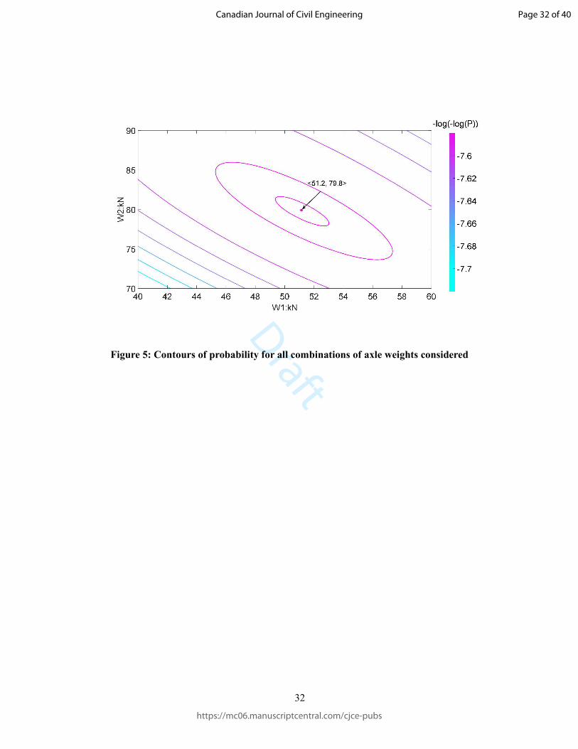
combinations can be obtained by Eq. 4 to Eq. 6. For this example, contours of probability are

plotted in Figure 5 for a typical vehicle for which the true weights are <W1, W2> = <51, 80> kN.

It is can be seen that the most probable result is at <51.2, 79.8> kN, which is very close to the true

value.

2.2.3 Results and Analysis

The procedures above are repeated for 200 simulated measurements. The mean errors and

standard deviations are obtained for the weights of each axle, gross vehicle weight (GVW) and

single axle weight, taken collectively for the two axles. The results from these simulations are

listed in Table 1.

Page 10 of 40



Draft

11

As can be seen, although the mean error and standard deviation of each entity are similar for

the two algorithms, both the mean error and the standard deviation are slightly less when applying

the pBWIM algorithm. For example, the mean error in the prediction of single axle weight

decreases from 0.23% to 0.17%, and the standard deviation decreases from 2.38% to 2.21%. The

biggest drop happens in the first axle. The mean error and standard deviation are reduced from

0.22% and 2.53% respectively to 0.15% and 2.27% when using pBWIM algorithm. Hence, for

the numerical model considering the random error in the influence line and measurement noise,

both algorithms are excellent with pBWIM improving the accuracy a little relative to Moses’

algorithm.

3. Field Test

In the simulations, most of the results were very good which made it hard to clearly identify the

differences between the two algorithms. For this reason, a field test was sought, for which the

results were poor. The objective was to determine if poor results from Moses’ algorithm could be

improved with pBWIM. The Šentvid Bridge in Slovenia was selected because it was located on a

stretch of road where the surface profile was not good and Moses’ algorithm was giving results

well below the level of accuracy that is typical of BWIM (Corbally and Žnidarič 2013).

3.1 Site Layout

The Sentvid bridge is a frame/culvert type of structure as shown in Figure 6. The bridge consists

of two independent structures, each of which is 6 m long and 6.25 m wide, carrying two lanes of

traffic.

The hardware components of the pBWIM system are the same as for conventional BWIM.

Each bridge structure is instrumented with 16 strain transducers, consisting of 4 FAD transducers

and 12 weighing transducers. Figure 7 shows the layout of the transducers for one bridge

structure. The FAD transducers (7-8 and 15-16) are mounted 4 m apart in the longitudinal

direction, two underneath each traffic lane. They are used for axle detection and speed calculation.

Page 11 of 40



Draft

12

The weighing transducers (1-6 and 9-14) are installed at mid-span with equal transverse spacings

of 0.5 m.

During the field tests, the test vehicles traveled in Lane 1 (corresponding to the slow-lane

shown in Figure 7). All the vehicles were pre-weighed at a static weigh station. There were 77

measurements recorded in total, as listed in Table 2.

3.2 Selected sensor

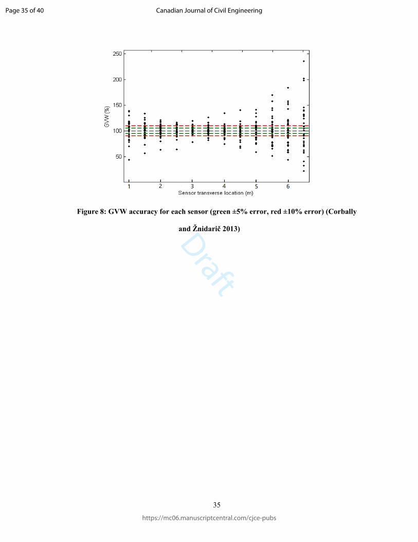
Comparing the accuracy of the calculated weights using individual sensors showed that the

sensors, which were located underneath Lane 1, in which all the trucks traveled, provided the best

accuracy. Figure 8 shows a comparison of the accuracy of the calculated GVWs where just one of

the weighing sensors is used in the BWIM algorithm in each case. The X-axis shows the

transverse spacings between the sensors used in the calculation and the Y-axis shows GVW

accuracy, with 100% indicating an exact prediction. The horizontal dashed lines correspond to the

goals set by Corbally and Žnidarič (2013) – see caption.

It can clearly be seen that the most consistent accuracy was obtained when the sensors

underneath the lane were used for weighing (notably, sensor 5 located at 3 m gave the best

accuracy). Some sensors give far more variability in the accuracy of the results (e.g. the

predictions from sensor 14 at 6.5m are very inconsistent). This results from the fact that the

sensors further away from Lane 1 have smaller magnitude and are therefore more sensitive to

noise/disturbances in the signals. Based on these results it was proposed that a single sensor

BWIM algorithm should be tested here using only sensor 5 for the weighing of vehicles in Lane 1.

It should be noted that accuracy might be improved by utilizing more sensors.

3.3 Measured ILs

The measured IL derived by the matrix method was adopted (OBrien et al. 2006). In this case, the

axle weights of the pre-weighed trucks and measured responses are known, so the IL ordinates

can be found by minimizing E in Eq. 1.

Page 12 of 40



Draft

13

As the Šentvid Bridge is an integral box culvert, vehicular load on the approach produces a

load effect on the bridge at mid-span. When calculating the measured influence line, an approach

length of 2 m is considered. Hence the total length of the influence line consists of bridge length

and two approaches, totaling 10 m (2 + 6 + 2 =10). Figure 9 shows the measured influence lines

for all test trucks.

It can be seen that all influence lines have a similar shape, and the peak values fall into the

approximate range [0.04, 0.07]. Figure 10 presents the histogram and a normal distribution fit to

the peak values. The data of Figure 10 matches well to a normal probability density function as

can be seen from the straight line fit of Figure 10b.

A Kolmogorov-Smirnov test (Massey 1951) is used to check every point in the influence

line for compliance with a specific normal distribution. Results show that 90% of all points in the

influence line follow a normal distribution at the 5% significance level. In this paper, it is

assumed that all influence ordinates follow the normal distribution. The calculated means and

standard deviations for each point on the influence line are shown in Figure 11.

3.4 Finding axle weights

In pBWIM, the procedure for determining axle weights from the measurements is similar to that

used for the numerical model. The process is illustrated in Figure 12. For each measurement, the

axle weights are first obtained with Moses’ algorithm. The Moses’ results are then used to

determine each approximate axle weight and hence to generate the range used to generate the

combinations to be tested in the pBWIM algorithm. Each axle weight is constrained to the range

[0.8, 1.2] times the corresponding Moses’ values, and the increment adopted is 0.1 kN. As the

influence line ordinates are normally distributed, the theoretical response, being a linear

combination, should follow a specific normal distribution for each combination of axle weights.

For each combination of axle weight, the mean ( k

iµ ) and standard deviation ( k

iσ ) of the response

Page 13 of 40



Draft

14

at scan i can be calculated by Eq. 3. The standard deviation of measurement noise ( Mσ ) is taken

here as zero. Using k

iµ and k

iσ , the probability of the response ( ( )kP R ) can be calculated using

Eqs. 4 to 6. Finally, the combination of axle weight ( PW ) with the highest probability is found.

4 Field Testing

4.1 Results with High-accuracy Influence Line

In an initial test, referred to as Case 1, a high-accuracy influence line (IL) is utilized. For this case, the

mean of all measured influence lines is used for both Moses’ BWIM algorithm and to find the mean

and standard deviation for the pBWIM algorithm. It is acknowledged that such a good IL would not

normally be available in real field conditions. For each measurement entity, the mean and standard

deviation of the relative mean errors are calculated and are listed in Table 3.

For this bridge, the results from Moses’ BWIM algorithm can be seen to be excellent. The

mean absolute error for each entity is greater when using the probabilistic algorithm, though the

corresponding standard deviation is less. For instance, the mean absolute error in the prediction of

the single axle weight increases from 0.022% to 3.58%; the standard deviation decreases from

13.31% to 12.45%.

To get an insight into the distributions of accuracy for the two algorithms, the details of

GVW errors versus vehicle number are plotted in Figure 13. This shows that most GVW errors

from pBWIM are less than (often ‘more negative than’) the errors from BWIM. When the GVW

errors are above zero, the predicted GVW’s from pBWIM are consistently less. Overall, the errors

in both algorithms are small and similar, with BWIM consistently outperforming pBWIM. The

likely reason is that the mean IL from all test trucks was used. As such, the uncertainty in the IL

was low. The potential for pBWIM to deal with IL uncertainty was therefore not realized in this

case.

Page 14 of 40



Draft

15

4.2 Results with Inaccurate Influence Lines

Based on the results from the first field test case, pBWIM does not have an obvious advantage

over conventional BWIM. However, it will be shown here that pBWIM can deal better with

inaccurate IL’s. To be more realistic, the IL is obtained here from a small number of calibration

test runs, and this low-accuracy IL is used to calculate the weights of trucks passing over the

bridge. In addition to the case already considered, two further cases are considered here for the

pBWIM and BWIM algorithms.

Case 2: The IL is taken here as the mean of the 10 measured ILs with the smallest peaks.

For pBWIM, two variations are considered. For Case 2a, the means and standard

deviations of the 10 ILs with the smallest peaks are used to calculate the probabilities.

For Case 2b, the same means are used but the standard deviations are based on all

measured ILs.

Case 3: Here the IL is taken from the 10 measured ILs with the greatest peaks. Similar to

above, Case 3a calculates the standard deviations from the 10 ILs with greatest peaks

while Case 3b calculates them from all measured IL’s.

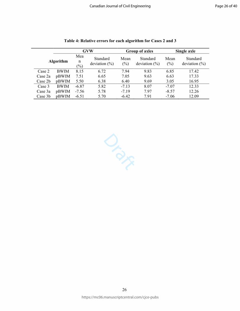
The results are listed in Table 4.

For Cases 2a and 2b, it can be seen that both the mean errors and the standard deviations

from pBWIM are less than the mean errors and standard deviations from BWIM. This is true for

all entities: GVW, groups of axles and single axles. It should be noted that the mean IL for

pBWIM is the same IL as used for BWIM. Clearly allowing for the variability in IL reduces the

sensitivity of pBWIM to influence line accuracy. Further, the standard deviation for IL used in

pBWIM is important as can be seen by the differences in accuracies between Cases 2a and 2b

(and similar for Cases 3a and 3b).

Page 15 of 40



Draft

16

For Case 3a, the mean absolute error from pBWIM is greater than the mean from BWIM,

but the standard deviation from pBWIM is less; For Case 3b, the mean absolute error and

standard deviation from pBWIM are both less than for BWIM.

In pBWIM, with the same mean of the measured IL’s, the more measured IL’s that are used

to get the standard deviations, the better pBWIM becomes, i.e., getting a good estimate of the true

standard deviation of the IL is important for pBWIM accuracy. For example, in Case 2b where

more accurate measures of the variability of the IL are used, the mean error with the pBWIM

algorithm falls to 5.5% for gross weights (from 8.15% with BWIM and 7.51% for Case 2a) and

there are similar reductions for axle groups and single axle weights.

For all cases, both BWIM and pBWIM based on measured ILs can get the best accuracy. It

can be inferred that BWIM and pBWIM will have similarly high accuracy if the data from the

calibration are sufficient, i.e., if the IL is accurate. In comparison to BWIM, pBWIM is better

able to cope with cases where the IL is not accurate.

5. Conclusion

This paper proposes a novel algorithm, probabilistic bridge weigh-in-motion (pBWIM), to

calculate axle and vehicle weights. Unlike conventional BWIM that minimizes the squared

difference between measured and predicted responses, pBWIM utilizes the probability of

measurement to find the most probable axle weights. Numerical modeling and field testing are

both used to evaluate the feasibility and accuracy of pBWIM. The simulations and measurements

are also used to find axle weights using Moses’ BWIM algorithm. Results of the simulations

show that both the mean absolute errors and standard deviations of calculated GVW, 1st and 2nd

axle weights are less for pBWIM in comparison to the corresponding values using Moses’

algorithm.

Page 16 of 40



Draft

17

In the field tests, when using the average of all measured ILs to find axle weights, the mean

absolute errors from pBWIM are slightly greater than the errors from BWIM, but the standard

deviations from pBWIM are less. When using IL based on a subset of available results, as would

be typical in a measurement campaign, pBWIM can get smaller mean absolute errors and

standard deviations, i.e., pBWIM appears to be more tolerant of the fact that the IL is inaccurate.

This paper provides a proof of concept for what is, to the authors’ knowledge, the first of its

kind – namely, an entirely probabilistic bridge weigh-in-motion system.

Acknowledgements

This research was supported by the China Scholarship Council, National Natural Science

Foundation of China (51178178), Science Foundation Ireland, the 7th Framework BridgeMon

project and Hunan Provincial Natural Science Foundation of China (13JJ2019). These programs

are gratefully acknowledged. Cestel, suppliers of the SiWIM BWIM system, is thanked for

providing access to the BridgeMon data.

References

Bakht, B., Mufti, A.A., Tadros, G., Eden, R. and Mourant, G. 2006. Weighing-in-motion of truck

axle weights by Japanese reaction force method. 3rd Int. In: Conf. on Bridge Maintenance, Safety

and Management, Porto, Portugal, July. 16–19.

Blab, R., and Jacob, B. 2000. “Test of a multiple sensor and four portable WIM systems.”

International Journal of Heavy Vehicle Systems, 7(2-3), 111-135.

Canadian Infrastructure. 2016. Canadian infrastructure report card - informing the future,

Available at:

Page 17 of 40



Draft

18

http://www.canadainfrastructure.ca/downloads/Canadian_Infrastructure_Report_2016.pdf#page=

28 [Accessed October 2, 2016].

Cardini, A.J. and DeWolf, J.T., 2007. Development of a Long-Term Bridge Weigh-In-Motion

System for a Steel Girder Bridge in the Interstate Highway System. University of Connecticut.

Corbally, R. and Žnidarič, A. 2013. Algorithm for Improved Accuracy Static Bridge-WIM System.

Deliverable D1.2, EU funded BridgeMon project (Bridge Monitoring), 2012 - 2014, GA no.

315629.

Deng, L., and Cai, C. 2010. "Identification of dynamic vehicular axle loads: Demonstration by a

field study." Journal of Vibration and Control, 17(2), 183–195.

Dowling, J., OBrien, E. J, and González, A. 2012. “Adaption of cross entropy optimization to a

dynamic bridge WIM calibration problem.” Engineering Structure. 44, 13-22.

Faraz, S., Helmi, K., Algohi, B., Bakht, B. and Mufti, A., 2017. Sources of errors in fatigue

assessment of steel bridges using BWIM. Journal of Civil Structural Health Monitoring, 7(3),

pp.291–302.

González, A. 2010. Development of a Bridge Weigh-In-Motion System. Germany: LAP Lambert

Academic Publishing AG & Co. KG.

González, A., Rowley, C., and OBrien, E. J. 2008. “A general solution to the identification of

moving vehicle forces on a bridge”. International Journal for Numerical Methods in Engineering,

75(3), 335–354.

Helmi, K., Bakht, B. and Mufti, A., 2014. Accurate measurements of gross vehicle weight

through bridge weigh-in-motion: A case study. Journal of Civil Structural Health Monitoring,

4(3), 195–208.

Jacob, B. 1999. COST 323 Weigh in motion of road vehicles. Final Report, appendix 1 European

WIM Specification, LCPC Publications, Paris.

Jacob, B., OBrien, E.J. and Jehaes, S. (Eds.) 2002, Weigh-in-Motion of Road Vehicles: Final

Report of the COST 323 Action, LCPC Publications, Paris, 538.

Page 18 of 40



Draft

19

Kalin, J., Žnidarič, A., and Lavrič, I. 2006. “Practical implementation of nothing-on-the-road

bridge weigh-in-motion system.” Proc., 9th Int. Symp. on Heavy Vehicle Weights and Dimensions,

ARRB Group, Vermont South, VIC, Australia.

Keenahan, J., OBrien, E. J., McGetrick, P. J., & Gonzalez, A. 2013. “The use of a dynamic truck-

trailer drive-by system to monitor bridge damping.” Structural Health Monitoring, 13(2), 143–

157.

Law, S., Chan, T. H., and Zeng, Q. 1997. “Moving force identification: a time domain method.”

Journal of Sound and vibration, 201(1), 1-22.

Lydon, M., Taylor, S., Robinson, D., Mufti, A., and Brien, E. 2016. “Recent developments in

bridge weigh in motion (B-WIM).” Journal of Civil Structural Health Monitoring, 6(1), 69-81.

Massey, F. J. 1951 “The Kolmogorov-Smirnov Test for Goodness of Fit.” Journal of the

American Statistical Association, 46(253), 68–78.

McNulty, P., and OBrien, E. J. 2003. “Testing of bridge weigh-in-motion system in sub-arctic

climate.” Journal of Testing and Evaluation, 11(6), 1-10.

Moses, F. 1979. “Weigh-in-motion system using instrumented bridges.” Transportation

Engineering Journal, 105(3), 233-249.

OBrien, E. J., Quilligan, M., and Karoumi, R. 2006. “Calculating an influence line from direct

measurements.” Bridge Engineering, Proceedings of the Institution of Civil Engineers, 159(BE1),

31-34.

OBrien, E. J., Rowley, C. W., González, A., and Green, M. F. 2009. “A regularised solution to

the bridge weigh-in-motion equations.” International Journal of Heavy Vehicle Systems, 16(3),

310-327.

OBrien, E. J., Znidaric, A., and Dempsey, A. T. 1999. “Comparison of two independently

developed bridge weigh-in-motion systems.” International Journal of Heavy Vehicle Systems,

6(1-4), 147-161.

Page 19 of 40



Draft

20

OBrien, E. J, Znidaric, A., and Ojio, T. 2008. “Bridge weigh-in-motion – Latest developments

and applications worldwide.” Proceedings of the International Conference on Heavy Vehicles

HVTT10, Eds. B. Jacob, E. OBrien. A. O’Connor, M. Bouteldja, Wiley, 2008, 39-56.

Richardson, J., Jones, S., Brown, A., OBrien, E., and Hajializadeh, D. 2014. “On the use of bridge

weigh-in-motion for overweight truck enforcement.” International Journal of Heavy Vehicle

Systems, 21(2), 83-104.

Rowley, C., Gonzalez, A., OBrien, E., and Znidaric, A. 2008. “Comparison of conventional and

regularized bridge weigh-in-motion algorithms.” Proc., Proceedings of the International

Conference on Heavy Vehicles, Eds. B. Jacob, E. OBrien, A. O'Connor, M. Bouteldja, Wiley,

2008, 271-282.

Rowley, C., OBrien, E. J., González, A., and Žnidarič, A. 2009. “Experimental testing of a

moving force identification bridge weigh-in-motion algorithm.” Experimental Mechanics, 49(5),

743-746.

Wall, C.J., Christenson, R.E., Mcdonnell, A.-M.H. and Jamalipour, A., 2009. A Non-Intrusive

Bridge Weigh-in-Motion System for a Single Span Steel Girder Bridge Using Only Strain

Measurements, Rep. SPR-2251, 7.

Yabe A and Miyamoto A. 2012. “Bridge condition assessment for short and medium span bridges

by vibration responses of city bus.” In: Proceedings of the sixth international conference for

bridge maintenance and safety, London, UK: CRC Press, Taylor and Francis Group, 195–202.

Yamada, K. and Ojio, T., 2003. “Bridge weigh-in-motion system using reaction force method”. In:

Proc. of the Int. Workshop on Structural Health Monitoring of Bridges/Colloquium on Bridge

Vibration. 269–276.

Yu, Y., Cai, C., and Deng, L. 2016. “State-of-the-art review on bridge weigh-in-motion

technology.” Advances in Structural Engineering, 19 (9), 1514-1530.

Page 20 of 40



Draft

21

Zhang, L., Haas, C. and Tighe, S.L., 2007. “Evaluating weigh-in-motion sensing technology for

traffic data collection”. In Annual Conference of the Transportation Association of Canada (pp.

1-17).

Zhao, H., Uddin, N., OBrien, E. J., Shao, X., and Zhu, P. 2013. “Identification of vehicular axle

weights with a Bridge Weigh-in-Motion system considering transverse distribution of wheel

loads.” Journal of Bridge Engineering, 19(3): doi: 10.1080/15732479.2014.904383.

Zhao, H., Uddin, N., Shao, X., Zhu, P., and Tan, C. 2015. “Field-calibrated influence lines for

improved axle weight identification with a bridge weigh-in-motion system.” Structure and

Infrastructure Engineering, 22(6), 721-743.

Žnidarič, A., and Baumgartner, W. 1998. “Bridge weigh-in-motion systems – an overview.”: Pre-

proceedings of the 2nd European Conference on Weigh-in-Motion of Road Vehicles, Eds. E. J.

OBrien & B. Jacob, Lisbon, Sep., European Commission, Luxembourg 139-151.

Žnidarič, A., Lavrič, I., and Kalin, J. 2008. “Measurements of bridge dynamics with a bridge

weigh-in-motion system.” Proc., 5th Int. Conf. on Weigh-in-Motion, B. Jacob, E. J. OBrien, A.

O’Connor, and M. Bouteldja, eds., ISTE Publishers, Paris, 388–397.

Page 21 of 40



Draft

22

Tables

Page 22 of 40



Draft

23

Table 1: Error percentages of mean and standard deviation for two algorithms

Entity Moses’ Algorithm pBWIM Algorithm

Mean (%)

Standard deviation (%)

Mean (%)


1st axle 0.22 2.53 0.15 2.27 2nd axle 0.24 2.22 0.18 2.16 GVW 0.24 2.21 0.18 2.17

Single axle 0.23 2.38 0.17 2.21

Page 23 of 40



Draft

24

Table 2 Distribution of test vehicles by axle number

Type 2-axle 3-axle 4-axle 5-axle 6-axle

No. trucks 8 8 7 52 2

Page 24 of 40



Draft

25

Table 3: Mean errors and standard deviation for each algorithm in Case 1

Entity Probabilistic BWIM Algorithm Moses’ BWIM Algorithm

Mean (%)


Mean (%)


GVW -2.39 5.91 -0.065 6.21 Group of axles -1.87 8.22 -0.49 8.61

Single axle -3.58 12.45 -0.022 13.31

Page 25 of 40



Draft

26

Table 4: Relative errors for each algorithm for Cases 2 and 3

GVW Group of axles Single axle

Algorithm Mea

n (%)


Mean (%)


Mean (%)


Case 2 BWIM 8.15 6.72 7.94 9.83 6.85 17.42 Case 2a pBWIM 7.51 6.65 7.05 9.63 6.63 17.33 Case 2b pBWIM 5.50 6.38 6.40 9.69 3.05 16.95 Case 3 BWIM -6.87 5.82 -7.13 8.07 -7.07 12.33 Case 3a pBWIM -7.56 5.78 -7.19 7.97 -8.57 12.26 Case 3b pBWIM -6.51 5.70 -6.42 7.91 -7.06 12.09

Page 26 of 40



Draft

27

Figures

Page 27 of 40



Draft

28

Figure 1: 2-axle truck passing over a simply supported beam

L=6m

2nd 1st

Beam Direction

Sensor

S

Page 28 of 40



Draft

29

Figure 2: Noisy and theoretical influence lines

Be

nd

ing

Mo

me

nt:

kN

m

Page 29 of 40



Draft

30

Figure 3: Simulated and theoretical responses at mid-span

Be

nd

ing

Mo

me

nt:

kN

m

Page 30 of 40



Draft

31

Figure 4: Flow chart for calculating axle weights using probabilistic algorithm and

comparing them to Moses’ algorithm

Generate 200 random 2-axle trucks

IL with random error Measurement noise

Simulated response

For all possible combinations of axle weights in the region of the calculated values by Moses’ algorithm

Get the probabilities of the corresponding responses

Axle weights are those with greatest probability

Get axle weights by conventional Moses’ algorithm for each vehicle

Calculate the mean errors and standard deviations for Probabilistic and Moses’ algorithm, respectively.

Page 31 of 40



Draft

32

Figure 5: Contours of probability for all combinations of axle weights considered

Page 32 of 40



Draft

33

Figure 6: Šentvid Bridge

Page 33 of 40



Draft

34

Figure 7: Plan layout of transducers (7, 8, 15, 16 for FAD, all others for weighing) unit: m

1

2

3

4

5

6

9

10

11

12

13

14

7

15 16

8

6

7

1 4 1

2.9

53

.41

0.6

4

11

1 ×

0.5

= 5

.50

.5

Lane 1

(Slow)

Lane 2

(Fast)

Page 34 of 40



Draft

35

Figure 8: GVW accuracy for each sensor (green ±5% error, red ±10% error) (Corbally

and Žnidarič 2013)

Page 35 of 40



Draft

36

Figure 9: Measured ILs

Longitudinal Distance: m

Re

sp

on

se

Page 36 of 40



Draft

37

(a) Histogram (b) Normal probability paper plot

Figure 10: Normal distribution fit to the peak value of the influence line

0.035 0.045 0.055 0.065 0.0750

5

10

15

20

25

30

0.035 0.045 0.055 0.065 0.0750.003

0.010.02

0.05

0.10

0.25

0.50

0.75

0.90

0.95

0.980.99

0.997

Pro

ba

bili

ty

Page 37 of 40



Draft

38

(a) Mean (b) Standard deviation

Figure 11: The means and standard deviations of measured influence line ordinates

0 2 4 6 8 10-0.02

0

0.02

0.04

0.06

0 2 4 6 8 10

10-3

1

2

3

4

5

6

Page 38 of 40



Draft

39

Figure 12: Flow chart of axle weight calculation using pBWIM

Calculate axle weights ( )

by conventional BWIM

Generate all possible combinations of ( )

in the region of the Moses’ values

For each possible combination, calculate the probability ( ) of

the measurement.

Get the combination of axle weights ( ) with

the greatest probability.

Page 39 of 40



Draft

40

Figure 13: GVW error for each vehicle with two algorithms

Err

or:

%

Page 40 of 40



Probabilistic Bridge Weigh-in-Motion · Draft 1 Probabilistic Bridge Weigh-in-Motion Eugene J....

Documents

Transcript of Probabilistic Bridge Weigh-in-Motion · Draft 1 Probabilistic Bridge Weigh-in-Motion Eugene J....