1

Privately-operated Water Utilities, Municipal Price Negotiation, and Estimation of

Residential Water Demand : The case of Francei

Céline Nauges and Alban Thomasii

E.R.N.A.-I.N.R.A., TOULOUSE

First draft

March 17, 1998

Abstract

This paper addresses the issue of price negotiation between a municipality and a private water

utility operator, and its implications for residential water demand estimation. Because negotiated

price may depend on municipality’s specific characteristics, competing forms of price

endogeneity have to be considered when using panel data. The impact of variables such as

average income, housing and system features is investigated both on municipal consumption

and price. We use efficient procedures to estimate a water demand equation on a panel of French

municipalities. Estimated price and income elasticities are significant and close to previous,

household-level studies.

2

INTRODUCTION

It is well recognized that estimating household demand for residential water is a prerequisite for

any water resource policy design. In cases where water resources are scarce and conflicting uses are

consequently more acute, it is important for the environmental regulator to assess properly the

expected changes in water consumption, following price or quota policy schemes. Even though

residential water demand may not appear the most important element in total water consumption,

public opinion is becoming more concerned with possible periods of restriction in use, as well as

trends of increasing water prices throughout Europe and the US.

Many empirical papers are dealing with estimation of residential water demand, most of

them in the U.S. Unfortunately, empirical results on important figures such as price and income

elasticities are very heterogeneous and remain often sensitive to econometric specification. Three

problems are not completely resolved yet in most cases. First, accurate data on prices paid (both

average and marginal) are not always available to the researcher, hence making it difficult to draw

relevant inference on consumers’ behavior. Second, demand shifters such as climatic and socio-

demographic variables should be included in these models. Third, when panel data are available, it

is not always the case that the additional information provided by pooling cross-sections with

times series is fully exploited by empirical researchers. In particular, it is important when using

panel data to assess the exact nature of price endogeneity in the consumption equation. As it

stands, endogeneity of water price may be caused either by instantaneous consumption entering

average price, or correlation between price and unobserved heterogeneity (individual effects), or

both. Incorrect model specification often leads to severe biases in demand elasticities. When

average or marginal price is correlated with individual effects in panel data, it may be the case that

private water utilities charge residential water prices depending on local communities’

characteristics such as average revenue, liabilities, or population density.

3

Hence, a possible cause of endogeneity of price in the demand equation is that the per-

head water consumption incorporates an unobservable individual effect. The latter can be

considered the unpredictable part of the consumption, in the sense that it is not captured by

explanatory variables introduced by the econometrician in the demand equation. If this individual

effect is correlated with price for water, be it marginal price or average price, then parameter

estimates are likely to be biased. The economic argument behind such a correlation is the

following. When negotiation takes place between the operator and the municipality, two major

variables are decided upon. First, the operator has to supply a determined level of drinkable water

to consumers in the community. Second, the price charged depends not only on the system

technical features, but also on expected, long-run per head water consumption. It is important to

note at this point that the price for water supply and treatment is decided upon by taking into

account all possible uses by the community, i.e. not only residential water use, but also industrial

and municipal uses. This is because industrials and municipal authorities will also be taking

advantage of the water system.

When a price regime is agreed upon, yearly changes in the marginal price may occur

because of technical features affecting the marginal cost of producing and delivering water to

consumers from facilities. The important aspect we stress however, is that the price regime

remains effective in the future. Similarly, per-head consumption moves around the expected long-

run level, because of income variations, local migrations, etc. Consequently, from an empirical

point of view, we may treat the unobservable component in the per-head consumption as an

individual effect for the local community. Endogeneity in the price of water may therefore be

present due to the possible correlation between the community-related price component, and the

community-dependent per-head consumption component.

The methodology of estimation proposed in the paper allows for a simple test for the existence

of a negotiation-driven price regime, which depends on some unobserved component in the per-

head consumption.

Another aspect of residential water demand worth investigating is the influence of

metering on individual consumption. In a situation where water is charged through a fee which is

4

computed on the basis of housing and/or household characteristics alone, it is likely that an

optimal use of the resource is not encouraged. On the other hand, when considering relatively

more significant marginal prices for water, the fact that actual water consumption is directly

charged to the individual consumer may provide the latter with enough incentives to reduce his

consumption, or at least converge to an optimal regime for consumption. This consideration is of

course related with moral hazard issues, in the sense that it is difficult to determine what

contribution the consumer has in total consumption of the housing. Given data on individual

housing density, as opposed to collective housing, it is possible to test for this metering effect.

This paper makes several contributions to the empirical literature on residential water

demand. First, we discuss the issue of price negotiation between the municipality and the private

operator, and its implications for residential water demand estimation. Second, we use adequate

consistent and efficient estimation procedures for the case of water demand with panel data.

Those instrumental-variable estimators have been but very rarely employed in the literature on

water demand.

The paper is organized as follows. Section II gives an overview of the literature on the

estimation of residential water demand. In Section III, we present a simple and intuitive economic

model of price setting and household demand for water. As this model will be estimated and tested

on French data for local communities, we introduce the section by a brief description of water

utilities in France. Data used, econometric methods, and estimation results are presented in

Section IV. Section V concludes.

5

II. OVERVIEW OF THE LITERATURE

The pioneering studies on residential water demand (Howe and Linaweaver, 1967; Gibbs,

1978; Danielson, 1979; Foster and Beattie, 1979) were mainly devoted to the US, where some

regions had been affected by periods of severe drought. As a consequence, economists have been

asked to look for the best way to regulate the demand side. Solutions include in particular rationing

of distributed water, education programs, awareness campaigns, and multi-part pricing policies or

increases in flat-rate prices. The 1980’s experienced an important increase in the number of

residential water demand studies (Billings, 1982; Schefter and David, 1985; Chicoine and

Ramamurthy, 1986; Nieswiadomy and Molina, 1989 among others), showing a larger interest in

economic analysis and econometric methods. Researchers in the current decade (Point, 1993;

Hansen, 1996; Agthe and Billings, 1996; Renwick and Archibald, 1997; Höglund, 1997) emphasize

new insights such as adoption by households of low-flow equipment, welfare consequences of a

price regulation and case studies of European countries.

Economists have always largely agreed on the variables to introduce in the water demand

function. The consensus is that, water having no close substitute in consumption goods, the only

price entering the demand function should be the price of water. However, Hansen (1996) shows

that in countries like Denmark where most of the residential water is heated (70% in

Copenhagen), the price of energy should also be considered. Price is not the only variable

affecting water consumption. Income, size of the household, house features (age of housing,

garden acreage, number of cars, domestic and sanitary appliances), weather variables may have a

non negligible influence.

If the choice of variables entering the water demand function has not led to much debates

among authors, consensus is still difficult to obtain on multiple-block pricing. In a multiple-rate

tariff framework, the consumer has to pay a fixed charge and a marginal price by cubic meter

depending on his level of consumption. It leads to a non linear budget constraint and a non linear

6

and a non differentiable demand function. In addition to the difficulties of deriving a demand

function, researchers disagree on the proper specification of the price variable. The consumer

faces few pricing blocks and consequently, few prices: the marginal price within each block and the

average price defined as total water expenditure divided by total water consumption. The

assumption of perfect information for the consumer advocates the introduction of the whole

price system in the demand function. However, some authors are suspicious about consumers

having perfect knowledge of the price system. Most models therefore either specify the average

price or the marginal price corresponding to the selected block, sometimes adding, following

Nordin (1975) and Taylor (1976), the « difference variable ». Specific to the multiple-part

pricing, the difference variable is defined as the difference between what the consumer actually

pays and what he would have been charged if all consumption units were charged at the marginal

price of the last unit of consumption. This difference variable should represent the income effect

embedded in the pricing schedule, an increasing tariff being seen as a tax on the first units

purchased, whereas a decreasing one simulates a subsidy. The coefficient of the difference variable

should then be equal in magnitude but opposite in sign to the coefficient of income. The Taylor-

Nordin price specification has received wide acceptance despite the fact that the previous

statement has been rarely verified, except in Schefter and David (1985) on simulated data.

The correct specification of consumer behavior when facing multiple-block pricing refers

to Burtless and Hausman (1978) and Moffitt (1986, 1990). These authors propose a two-stage

model in which the consumer first selects the block, and then maximizes his/her utility subject to a

budget constraint. Hewitt and Hanemann (1995) are among the rare authors to use this kind of

two-step model in water demand studies. To simplify the expression of the demand function,

researchers often only consider the block where most consumers are located (a selection bias can

emerge) or simply omit the choice of the block by the consumer (can lead to a simultaneity bias

because the consumption depends on price but price depends also on block and so on quantity).

Multiple-rate pricing consequently renders the economic analysis difficult: not taking into account

the specificity of the pricing structure can generate two kinds of bias and a whole description of

7

the consumer choice heavily rests on the perfect information assumption and makes the

econometric treatment more difficult.

Econometric methods are often discussed in water demand studies. The question of

endogeneity clearly emerges when researchers choose to introduce as a regressor the average price

of water. Depending largely on total water consumption, it can produce a bias of simultaneity

because total water consumption is encountered in the two sides of the equation. If the

orthogonality condition between the regressors and the error terms fails, Ordinary Least Squares

(OLS) technique leads to biased estimates. The endogeneity bias should then be corrected by using

Instrumental Variable (IV) estimators, which, together with simultaneous equations, are being

more and more commonly employed in recent water demand studies. OLS and IV procedures are

inappropriate techniques when the consumer's behavior is described by a two-stage model, or in

the case of panel data. The two-step representation of the consumer's choice requires Maximum

Likelihood (ML) estimation procedure whether panel data should be treated with specific methods.

To our knowledge, Höglund (1997) was the only one to use such techniques on panel data for

Sweden.

Despite the difference among econometric methods and various kinds of available data

(cross sections, time series, or both), economists generally agree that water demand, with respect

to its price, is inelastic but not perfectly so. It seems also widely accepted that, in addition to

price, variables such as income and size of the household have significant positive effects on water

consumption. Table 1 presents a summary of the most often quoted studies, including details on

data used, econometric methods, and the results in terms of price-elasticity.

Recent research on residential water demand emphasize new insights such as the possible

complementarity between water and energy. Hansen (1996) shows that in Denmark, water

demand is more sensitive to the price of energy than to its own price, due to the wide utilization

of heated water. The study by Agthe and Billings (1996) is largely devoted to the adoption by

households of new equipment such as low-flow faucets, low-flow shower-heads and drip irrigation

8

for gardening. Endogenous technological change is also at the core of the Renwick and Archibald's

(1997) paper. Highly desegregated data enable these authors to complete their study with some

welfare analysis. In particular, they emphasize the higher sensitivity of low-income households to

an increase in the price of water. Finally, numerous studies in the 1990’s were devoted to

European countries, e.g. France (Point 1993), Denmark (Hansen 1996), Sweden (Höglund 1997).

Despite the relative similarity of results regarding the sign and magnitude of the price-elasticity of

water demand for several types of data, economic assumptions and econometric methods should

ideally be conducted using repeated survey data from individual households, with appropriate

econometric methods.

III. ECONOMIC CONSIDERATIONS

One of the main purposes of studying residential water demand is the estimation of the

price-elasticity of demand. This requires carefully designed econometric methods in order to

produce unbiased parameter estimates, hence unbiased price-elasticity estimates. When estimating

residential water consumption, one should pay a particular attention to the definition of price and

the way it is determined. In the case of private companies operating water utilities through a

contract with the municipality, the price (marginal and average price) is commonly the result of a

negotiation between the municipality and the private operator. Price is decided for the whole

contracting period and will largely depend on the expected consumption regime of the

municipality. The fact that the price is not solely derived from a profit maximization rule but is

the outcome of a negotiation makes the analysis of the local community residential water demand

more complex. A full comprehension of the determination of the water price in a municipality is

a prerequisite for correctly estimating the water demand function of this local community. In

what follows, we describe in more detail the French context in terms of water service and the way

price for residential water is negotiated upon.

THE FRENCH WATER MARKET

9

The French 36,551 municipalities are responsible before the law for the satisfactory

operation of local water services (supply, treatment and sewage). National legislation requires that

adequate (both in quantity and quality) water resources be supplied to every potential user in the

local community. In practice, municipalities can decide to operate water utilities by themselves

(possibly in association with other local communities) through a local, public water authority.

They may also prefer to delegate management of water services to a private company. In both

cases, the local community may associate with others, especially when the community is small, to

share a common water system or to benefit from economies of scale in operating some of the

services.

It must be noted that the water system (main pipelines, service connections, reservoirs,

treatment facilities,...) is still publicly owned by the municipality, even if it delegates operation

and possibly investment in additional facilities to the private operator. Contract-based

relationships between the municipality and the private operator are the rule, and conflicts are

resolved through the prevailing legal system. There are no central regulation authorities

concerned with managerial and legal aspects of water supply. On the other hand, local and

national environmental protection agencies may control for environmental aspects related to the

service (effluent emission standards in particular). The French system is therefore different from

what is found in Great Britain and in the US. In Great Britain, all water utilities are now privately-

owned since the mid-1980’s. Concentration in the water supply industry led to the creation of 10

major regional companies, that are regulated by an independent agency (OFWAT). The OFWAT

designs a price-cap policy directed to all 10 private companies.

In the US, about 46 percent of water utilities were public, and about 28 percent were

privately owned in 1992. Private utilities are subject to public regulation, through state

commissions, boards or municipal governments, whereas most public water utilities are not subject

to regulation. Public regulation objectives are to adequate and safe service to customers in the

local community, and to ensure that service rates are reasonable and fair, given a reasonable

efficiency of the system. To do so, public regulation authorities regularly control utility rates of

return and base rates (see Beecher 1997).

10

In the case of France, it is well recognized that most municipalities prefer to delegate

water services when they lack technical know-how and, above all, when their financial burden has

become too acute. There are several reasons for this sharp increase in liabilities related to water

services. First, deterioration in the quality of groundwater has led the government to impose more

stringent quality standards. In order to comply with these standards on distributed water quality,

municipalities may have to expand their treatment capacities, or invest in new ones. Second, the

European Commission directives on water treatment and wastewater treatment plants require that

the vast majority of local communities be properly equipped with such facilities before 2005.

Third, the 1992 French Water Act imposes new restrictions on the management of water services

by local communities, in the form of a separation in the municipality budget between water

services and the other services. Consequently, since the budget for water services has to be

balanced, financial transfers from general community taxes or other revenues to these services

become impossible. Hence, a private operator may be preferred to a purely public management

option, even if the price of water may be higher as a consequence.

The two major private companies dominating the French water supply market are the

« Compagnie Générale des Eaux » and « Lyonnaise des Eaux ». Table 2 presents the relative

importance of private and public operators in French municipal water services in 1993.

PRICE NEGOTIATION BETWEEN MUNICIPALITY AND THE PRIVATE OPERATOR

When a private company is chosen by the municipality for managing and operating the

water utility, the private firm and the local community decide on the price by mutual consent.

More precisely, the relationship between the municipality and the company, which has a local

monopoly power is formalized by means of a contract. Considering negotiation on price for

water, it is more adequate to refer to water « rate » rather than to water « price ». Indeed, the

negotiation ultimately determines the whole rate structure, i.e. both the type of tariff (linear, two-

part, increasing-blocks, decreasing-blocks) and the water price charged by unit consumed, for each

class of users (farmers, households, industrials).

The municipality and the private operator agree on three different elements: a basic tariff,

a formula for annual price revision, and clauses allowing for exceptional conditions. The basic

11

tariff and the formula for the price revision are determined a priori for the period of the contract.

A formula for annual price revision is necessary because the private operator bears operating costs

that are affected by variations in input prices and productivity earnings. Moreover, it is also true

that exogenous shocks on water demand may affect operating conditions (peak periods).

Consequently, the legislation has introduced the possibility of updating the contract terms when

appropriate.

The negotiation between the municipality and the private operator is essentially directed

on the determination of the basic tariff. The community’s water service board and the private

firm have to agree on a price policy that achieves budget balancing for the private operator, while

remaining consistent with the orientation of the tariff policy chosen by the municipality. The

budget-balancing requirement means that the price charged to water users has to cover both

operating and investment costs. Fixed costs consist basically of water system features (system

size, importance of leaks among others); variable costs depend essentially on actual water

consumption. The prediction of future consumption levels hence plays an essential role during the

negotiation. The second element is the orientation of the local tariff policy: the water rate

structure and the price charged by unit of consumption are proposed by the municipality

executives in charge of water services, according to the municipality objectives.

Let us consider some examples of tariff policies for residential usersiii. First, a uniform

tariff aims at ensuring equal treatment to all residential users. Second, a two-part tariff (a service

charge corresponding to access to water supply, plus a price per unit of water consumed) is the

closest picture of the costs incurred by the water service. The service charge corresponds to fixed

costs supported by the operator, while the price per unit consumed corresponds broadly to

Operation and Maintenance (O&M) costs proportional to water actually supplied and consumed.

This type of tariff, which reflects relatively well the expenses incurred for each customer supplied,

meets the equity concern. However, in cases where the treatment and supply units reach a point

of saturation, the two-part tariff fails to indicate to residential users that an increase in

consumption would induce additional investment costs. Third, the proportional tariff (no service

12

charge, and a constant price by unit consumed) is the simplest tariff for residential users. However,

this system does not provide consumers with proper incentives. By fully reporting fixed costs on

every unit of consumption charged, the proportional tariff does not accurately indicate the

variation in costs induced by a variation in overall water consumption. Finally, the increasing

tariff is sometimes advocated in that it better protects the water resource. It can also be

recommended as a mean of redistributing incomes from consumers with a greater water

consumption toward consumers with a more modest consumption.

We can easily imagine that municipality’s policy orientations are implemented according

to two major steps. First, global priorities are defined in terms of broad categories of users; the

municipality may for instance favor residential water consumers, promote urban development, or

encourage industrial settling in the community. Second, policy objectives apply within each

category of users.

ECONOMIC MODELING

The determination of the basic tariff for residential users therefore reduces to a function of three

variables: system features, expected water consumption, and objectives of the tariff policy. As

choices made by municipalities depend on numerous factors, we consider that policy orientations

are predominantly determined by some socio-demographic characteristics of the local

communities. In other words, we assume that choices of the municipality and the private operator

are made according to, for example, industrial activity, dominant activity (industry, farming) on

the local community territory, population density, or the distribution of incomes in the

municipality.

Let us introduce some notation. Socio-demographic community-related characteristics are

denoted ZP , N are system features, C0 is expected future residential consumption regime.

Define P P N C ZP0 0 0= ( , , ) as the basic tariff negotiated for the residential users. P0 represents

the whole price structure, including marginal price(s) and possibly fixed service charges. Finally,

13

let C t and Pt respectively denote the actual consumption level and the rate for water (that is

actually charged in the municipality) at time t.

Differences between Pt and P0 may occur in practice during the planning period,

depending on two major categories of factors. First, from the supply side, future changes in input

price levels need to be accounted for in the contract between the municipality and the private

operator. A simple actualization rule is employed, letting changes in water price depend on input

price indexes (labor cost, construction cost, energy,...) through a multiplicative coefficient applied

to update price. Let k denote that revision (updating) coefficient. k is equal to 1 if no revision is

necessary. Second, on the demand side, changes in future demand levels affect operating and

maintenance costs as well, even if input price are unmodified, simply because the scale of activity

is modified. Such a change in demand is reflected in the gap between actual consumption C t and

the expected consumption regime, C0 . At every period t, price has to adapt (even slightly) to the

change in demand around the consumption regime C0 , so as to equate instantaneous marginal

cost of the service with marginal price for water.

Price Pt thus reads:

Pt = k .P0(N ,C0, Z P ) + P(Ct − C0 ), (1)

where the first term is the price regime, possibly modulated by input cost changes if k is different

from 1. The second expression in the right-hand side above accounts for the modification due to a

change in demand from the expected consumption regime. Note that since P0 is a price structure,

not a single price measure, it is clear that changes in Pt will affect both marginal price and

possible fixed service charges.

As explained above, determinants of the municipal price policy are numerous and

sometimes complex. Municipal choices may be influenced by other elements such as local lobbies

or the water service existing liabilities. It is also true that these choices are likely to be related to

socio-demographic variables of the municipality. Using socio-demographic, municipality-related

variables to proxy determinants of the price policy is certainly a necessary simplification in the

14

absence of more accurate data. Let u denote the part of the price regime unexplained by the Z P

variables, so that price charged at time t to residential users becomes

Pt = k .P0(N ,C0, Z P ) + P(Ct − C0 ) + u . (2)

When negotiating on a contract for water services, both the municipality and the private

operator have to make the best prediction of the consumption regime for the next years, and try

to anticipate the consumption of each class of users. We focus here only on the residential users’

consumption regime C0 , assumed to be largely determined by some of the characteristics of the

local community such as average income in the municipality, average housing size, type of

housing (individual or collective housing), average housing equipment. Let ZC denote such

municipality-related characteristics, so that C0 = C0(Z C) .

At each period t, actual consumption C t deviates from the expected consumption regime. These

differences can be due to severe climatic conditions, a non expected variation of income or may

follow from local migrations. Let X t denote these household-dependent variables, so that actual

consumption at time t is

Ct = C0 (ZC ) + C(X t ,Pt ) . (3)

As in the price equation, we have to specify an individual termα representing the consumption

regime that is not explained by variables ZC .

The final model specification is: Pt = k .P0 N, C0(ZC ),ZP[ ] + P(Ct − C0) + u (4)

Ct = C0 (ZC ) + C(Xt ,Pt) + α (5)

Note that the same ZC variables appear at two different places in the consumption

equation above, as price depends on the expected consumption regime and therefore on the ZC ’s.

Redundant variables could also be found if some of the socio-economic characteristics directly

entering the basic tariff determination are also related to the consumption regime, i.e. if the ZP

and ZC vectors have elements in common. This could be true of the income variable for

instance. The consumption regime is commonly affected by the level of income and average

15

municipality household income could also be one of the central variable determining the tariff

policy of the local community.

Also, some variables omitted from the price regime equation could be as well omitted from

the consumption regime equation. As a consequence, α and u would be correlated. Suppose for

example that the local community has the objective of promoting industrial developments in its

local area. This could have as a consequence, when negotiating the contract, a policy of cross

subsidies favoring industrials and penalizing residential users, thus affecting the price regime for

domestic consumers. On the other hand, the settlement of new industries could lead to a growing

local population, hence to a higher, unexpected consumption regime for the local community.

To conclude this section, it is essential to keep in mind that the price (either average price

or marginal price) is not exogenously given to the municipality. The local community, because of

its expected-consumption regime, its specific socio-demographic characteristics and possibly

pressure groups influence the price which is then charged to its consumers. An important

consequence is that, when focusing on the estimation of residential water demand, some variables

could simultaneously enter the price function and the consumption function. This may lead to

biased estimates if such a simultaneity is not taken into account.

IV. EMPIRICAL APPLICATION

DATA DESCRIPTION

We use a panel data sample of 116 local communities in eastern France, on the period

1988-1993 (T, the number of time periods is 6). These 116 municipalities are supplied by the

Compagnie Générale des Eaux, a major private operator (see Section III), which provided us with

annual records on aggregate residential consumption (by local community), detailed prices and

various technical data on water system features. In the area considered, multiblock pricing only

applies to industrials. Consequently, the price policy corresponds to a two-part tariff. For each of

the 116 local communities, socio-economic information is obtained from the 1990 French census

16

(INSEE 1994). Temperature and rainfall measures are collected from the local meteorological

authority (Meteo-France). Summary statistics for variables are presented in Table 3.

Before estimating the residential water demand function, we test for the assumption that

the price regime is influenced by the system features and the socio-economic variables. We

therefore use both marginal price and average price to test for this influence. Equation (4) gives

the price for a representative municipality. Estimation of this equation requires introducing the

usual econometric residual. Let i denote the municipality index, t the time period index. The price

equation thus becomes

Pit = k .P0 Ni ,C0(Zi

C), ZiP[ ] + P(Cit) +ui + uit , (6)

where ui and uit are the community-specific and econometric, time-varying residual

respectively.

The main component of the price charged at date t is the basic tariff Pi0 and we assume

that the component P(Cit) is negligible in the current water price and thus can be included in the

last error term uit . The form of the basic tariff function being unknown, we assume a linear form.

We therefore estimate the following equation:

Pi = α 0 + α1 .Ni + α2 .Z i + ui i =1, 2,..., N

with Pi =1

TPit

t∑ ; Ni =

1

TNit

t∑ and Zi = (Zi

C , ZiP ).

Pit is either marginal or average price of water in community i at time t ; N it is the vector of

water system features, including both the number of service connections (CO) and the number of

leaks detected (LEA). The Zi -vector includes the population density (DEN), the industrial

activity rate (ACT), the proportion of private housings (HOU), the proportion of recent housings

(H82), and the average household income (I).

Estimation results for the average price case are presented in Table 4. Similar results were

obtained with the marginal price as the dependent variable and are not reported here. Estimated

17

standard errors are computed using the White heteroskedasticity-consistent variance-covariance

matrix.

It can be seen that income and the proportion of recent housings have a significant and

positive effect on price charged in average on the period, in each local community. We therefore

find evidence that there is a significant influence of some socio-economic characteristics of the

local community on the water price charged in this community. The number of leaks detected, a

variable which reflects the magnitude of maintenance and replacement costs, has also a positive

effect on price. Consequently, endogeneity of both marginal and average price has to be checked

carefully when estimating the residential water demand function.

ESTIMATING DEMAND : PANEL DATA ECONOMETRIC METHODS

The residential water demand consumption equation to be estimated is

Cit = Xit .β + ZiC .γ +α i +ηit (7)

where Cit represents water consumption in the local community i at time t;

X it is a vector of demand shifters including the price of water, some socio-economic and

climatic variables, depending both on local community and the period;

ZiC is a vector of community-specific socio-economic variables;

α i is the unexpected water consumption regime

and ηit is the usual econometric residual.

As discussed in section III, the municipality-specific consumption regime is explained by

variables ZiC , and deviations from this regime are determined by demand shifters X it . The α i

and ηit error terms are assumed to have both zero mean. Since both time-varying and

community-specific regressors are present in the demand equation, appropriate panel data

methods are required to estimate model parameters. Furthermore, the estimation method

18

employed will have to be adapted to the joint presence of error components in the form of

residuals and of individual (community-related) effects.

There are two possible sources of endogeneity in the equation above. First, as emphasized

in section III, ZC variables could be redundant in the consumption equation, leading to an

endogeneity bias because of the correlation between some explanatory variables and the error

term ηit . This possible source of endogeneity has to be tested for by performing a test of

exogeneity restrictions. The Hausman test uses the fact that the Least Squares estimator on a

transformation of variables in Equation (7) (taking deviations from individual means, i.e. « Fixed-

Effects » or « Within » estimation) are consistent and asymptotically efficient under the null

hypothesis that explanatory variables are exogenous. It will however be inconsistent under the

alternative. On the other hand, an Instrumental Variable estimator (IV) is consistent under both

the null and the alternative hypothesis, but it will not be asymptotically efficient under the null.

Under the null hypothesis that exogeneity restrictions are valid, the Hausman test statistic has an

asymptotic chi-square distribution with degrees of freedom equal to the number of explanatory

variables.

Second, endogeneity in the model may be present when the specific, community-related

unexpected component of the consumption regime α i is specified as a random component, and is

correlated with some model regressors ( Xit , ZiC ). We then consider a « Random-Effects » panel

data model, which requires Generalized Least Squares (GLS) estimation method. As in the first case

above, the Hausman exogeneity test statistic may be computed, by comparing the GLS and the

« Within » estimator. GLS estimates will be both efficient and consistent if no community-

specific characteristic has been persistently omitted or, in econometric terms, if the individual-

specific effect is not correlated with explanatory variables. If this assumption fails, then the

random-effects estimator will not be consistent and Within estimates have to be considered. It

remains that coefficients of the time-invariant variables ZC are not identified (when deviating

the variables from their individual means, the time-invariant variables are eliminated). Hausman

19

and Taylor (1981) propose a IV estimator adapted for models with both time-varying and

individual-specific regressors. Let index 1 denote exogenous variables, index 2 denote endogenous

explanatory variables. Regressors are decomposed into k1 time-varying exogenous variables, k2

time-varying endogenous variables, g1 individual-specific exogenous variables and g2 individual-

specific endogenous variables. The Hausman-Taylor (HT) estimator is based on the following

matrix of instruments, written in matrix form:

A = QX ,X1, Z1C[ ] ,

where QX = Xit − Xi for all i and all t and the resulting HT estimator is

ˆ δ HT = ( ′ Φ Ω −1/2 PAΩ− 1/2 Φ)− 1( ′ Φ Ω−1/ 2PAΩ−1 / 2C) ,

with PA = A(A' A)−1A' and Ω ≡ E(α + η)(α +η)' .

$δHT is the vector of parameter estimates corresponding to initial parameters ( )β γ, , Φ is

the NT × (k1 + k2 +g1 + g2) -matrix of explanatory variables X1, X2 ,Z1C ,Z2

C( ), C is water

consumption (dependent variable) and PA is a projection matrix. The Ω−1 2/ matrix takes into

account heteroskedasticity specific to panel data models. The identification condition requires

that the number of exogenous time-varying variables be greater or equal to the number of

endogenous time-invariant variables.

Amemiya and MaCurdy (1986) propose a more efficient IV estimator, adding a new set of

instruments in the form of a matrix denoted X1* . This matrix is obtained by replicating each line

of the matrix X1 T times. The matrix of instruments suggested by Amemiya and MaCurdy is

therefore AAM = QX, X1* , Z1

C[ ] and the identification condition in that case becomes Tk1 ≥ g2. The

intuition behind this estimator is that, if X1 is exogenous in the sense that we have

E(X1 itαi) = 0 ∀i , then the individual effect α i should also be uncorrelated with X1 at every time

period (i.e. before and after the current period considered).

20

More recently, Breusch, Mizon and Schmidt (BMS, 1989) demonstrate that a more

efficient estimator can be derived by choosing as instruments the matrix

A BMS = QX,(QX1)*,(QX2)*, BX1,Z1C[ ]

where BX = Xi for all i, with the identification condition becoming Tk1 + (T-1) k2 ≥ g2. The

argument for this estimator is stronger than for the AM estimator. BMS argue that if endogeneity

is caused by a correlation between explanatory variables X2 and the individual effect only, then

the components in X2 that vary over time but are independent from individual effects are also

valid instruments.

DEMAND ESTIMATION

We now estimate the residential water demand function defined in (7). The X-vector

(regressors that vary over both i and t) consists of price variables (AP, MP), average taxable

income (I) and the total amount of rainfall during the year and during the three summer months

(TOTRAIN, RAIN). The Z-vector of time-invariant (community specific) regressors contains all

other socio-economic variables. All variables are in logarithmic form. Specific panel data methods

will be employed in order to answer to five main questions:

1) Do consumers respond to average price or to marginal price for water ?

2) Are marginal and average prices exogenous or endogenous variables ?

3) Are there municipality-specific effects that have been omitted in the explanatory

variables ?

4) Do socio-economic and climatic conditions have significant effects on water

consumption ?

5) Does individual metering matter ?

In order to determine which price variable consumers respond to (marginal, average, both

or none), we estimate the water demand function including a decomposed price variable, following

Opaluch (1982). The average price is decomposed into the marginal price and a second price

21

variable equivalent to the average price less the marginal price. The price decomposition is, in our

case, simplified because of the linear pricing structure. We have AP= MP + (AP-MP). The model

estimated is thus of the form:

C = f (MP, AP − MP, I, RAIN ,ZC) (8)

In a first step, we compute the tests described earlier to determine the appropriate

estimator for model parameters. The first Hausman test checks for the exogeneity of the price

variable. Within estimates are reported in Table 5. In a second step, instrumental Within

estimation is performed. The instruments chosen are exogenous time-varying variables: the

number of service connections (CO), the number of leaks detected (LEA), the size of the water

system (NET) and the two weather variables (RAIN, TOTRAIN). The Hausman test statistic is 3.6,

a value below the χ2 (4) critical value at the five percent level of confidence (9.49). We thus

conclude in favor of the exogeneity of the price variables.

A second Hausman test is performed to check for the presence of individual-specific

effects. GLS estimates are reported in Table 5. The Hausman test statistic is 61.9, which

significantly exceeds the critical value for the χ2 (4) at the five percent level of significance

(9.49). The test « Within vs. GLS » hence rejects the null, and therefore accounts for endogeneity

in the equation under scrutiny. The assertion made in the economic part is thus verified on our

data: there exist persistent omitted explanatory variables in each municipality.

Results of the test call for the use of specific IV estimation procedures as proposed by

Hausman and Taylor (HT), Amemiya and MaCurdy (AM) or Breusch, Mizon and Schmidt (BMS).

The three estimators are computed with the associated Hausman tests, in order to check for the

exogeneity assumption and the validity of the instruments chosen in each case. We assume here

that X1 contains the average taxable income (I) and the two rainfall variables (RAIN and

TOTRAIN) ; all three variables are initially assumed not to be correlated with the individual error

term α i . X2 contains the price variables (MP and AP-MP). Z1 is assumed to contain all other

socio-economic variables while Z2 is assumed null. The Hausman test statistics reveal that

industrial activity rate (ACT) is correlated with the individual error term. This variable is therefore

22

eliminated from the instruments and included in the Z2 -vector. One possible explanation for the

endogeneity of this variable is that the activity rate is a proxy for the municipality liabilities;

these liabilities are not available to us and are likely to be correlated with α i . After eliminating

the activity rate from the matrix of instruments, all three Hausman tests confirm the correctness

of our choices. We only report in Table 5 the BMS estimates, as they are the most efficient, and

yield estimates that are numerically close to HT and AM estimates.

We now consider the tests proposed by Opaluch (1982). The parameter associated to

marginal price,β1 , is -0.072 whereas the coefficient of the second price variable, β2 is equal to

-0.216 (see Table 5). Both are significantly different from zero. The test statistic associated with

the equality restriction for these parameters is β2 − β1( ).(var(β2 − β1))−1 / 2[ ] , which is normally

distributed under the null. The test statistic is equal to 4.15, which exceeds the critical value of

1.96 at the 5% level of significance. Therefore, neither the marginal price model nor the average

price specification can be rejected.

This result can be explained by the fact that the correlation between the marginal and the

average price is close to one. This significant correlation is linked to the overwhelming part of

marginal price in the average price. If we decompose the average price as the sum of the marginal

price and the ratio [fixed charges over total quantity consumed], it appears that the former is

largely superior to the latter.

Therefore, we consider a second specification for the residential demand equation, in

which the only price variable is average price. Moreover, household water expenditures in France

represent on average 1.5 to 2 percent of households net income, and few consumers know the

marginal price of water whereas most of them remember their last water utility bill. The average

price model is of the form

C = f (AP, I, RAIN , ZC) (9)

Estimation results for this model are presented in Table 6. The five Hausman tests lead to

the same conclusions as for Equation (8) that is, exogeneity of the explanatory variables and

23

among them the average price of water, and the presence of local community-specific effects.

Exogeneity of average water price could appear surprising at first, but if we recall the result above

concerning the high degree of correlation between marginal and average prices, the explanation is

clear. The component of average price depending on total water consumption is negligible in

regard to the marginal price.

Let us comment on the results concerning the other explanatory variables. We will

consider parameters estimated by the BMS procedure, as this method allows for identification of

all parameters and is the most efficient IV estimator. The parameter associated with average price

is significantly different from zero. Consumers would respond to changes in the average price of

water by lowering consumption by about 22% of the relative change in the average price. The

price-elasticity of -0.22 is close to the value estimated by Point (1993) on France (-0.17).

Average taxable income has a statistically significant positive effect on the consumption of water

(around 0.1). It is important to note that the local communities in which the proportion of recent

housings (built after 1982) is large use relatively less water, all other things equal. The explanation

can be the lower age of existence of the system pipes, hence reducing the probability of leaks. The

results also emphasize that local communities in which more housings are equipped with a bath tub

consume much more water than communities where housings are more largely equipped solely

with a shower or a washbasin. Hence, inside consumption seems to dominate in the total amount

of water consumed. In other words, the share of water intended to sprinkling is small in this region

of France. This fact can be related to the non-significant rainfall variable.

An interesting result concerns water meters. Living in an individual housing has a

statistical significant negative effect (-0.44) on water consumption. The presence of individual

water metering has therefore a non negligible influence. To this respect, many public and private

operators in France have considered a generalization of water metering systems in the near future,

to provide consumers with incentives for adequate day-to-day management of their water use.

OLS estimations are also performed on Equations (8) and (9). OLS coefficients are rather

similar to the ones estimated by specific panel data methods. The reason is that, explanatory

variables being exogenous, no bias of simultaneity occurs.

24

V. CONCLUSION

Many empirical papers dealing with the estimation of residential water demand largely document

the endogeneity issue of average price in the demand equation. When using aggregate data on a

panel of municipalities, it is important to determine precisely the source of price endogeneity,

which may be due to local community effects. The way price is negotiated between the

municipality and the private operator is an important determinant of water consumption trends,

and it often depends on expected consumption regime at the local community level for the

planning period. Consequently, socio-demographic variables appear both as water demand shifters

and as determinants of the municipal price regime.

In the case of France, many water utilities are privately operated, though publicly owned. In that

case, water price is negotiated between the local community and a private operator for a given

planning period. Local community-dependent variables such as average income and average

housing characteristics are determinant in the setting of price rates and contract terms.

This paper proposes a model of water price determination in the case of a private

company operating a municipal water utility. We highlight in particular the importance of

expected consumption per head within the municipality in the price policy adopted. The model is

estimated using a panel sample of French municipalities. Estimation results indicate that

households respond to both average and marginal prices, with a significant but low price elasticity

of -0.22 in the case of average price. A significant income effect is also found, with an income

elasticity estimated at 0.1. Furthermore, residential water consumption is significantly lower when

individual housing with meter recording is dominant. This result advocates for the development of

water metering in collective housings.

As far as policy implications for regulating the demand side are concerned, it is not immediate

that a price policy would induce a substantial reduction in residential consumption. Indeed,

residential demand appears poorly sensitive to price variations. Hence, non-price policies such as

25

low-flow equipment promotion, awareness campaigns and education programs should also be

considered. Short-run determinants of residential water consumption are now well established and

should be completed by long-run considerations. In particular, household equipment in durable,

water-consuming goods could be targeted by policy makers. Subsidy programs for low-flow

facilities and new technology adoption may prove useful to complement price policies in periods

of severe water shortages.

26

REFERENCES

AGTHE, D.E., and R.B. BILLINGS [1996], « Water-Price Effect on Residential and Apartment

Low-Flow Fixtures », Journal of Water Resources Planning and Management, 20-23.

AMEMIYA, T. and T.E. MACURDY [1986], « Instrumental-Variable Estimation of an Error-

Components Model », Econometrica, 54(4), 869-880.

AHN, S.C. and P. SCHMIDT [1995], « Efficient Estimation of Models for Dynamic Panel Data »,

Journal of Econometrics, 68, 5-27.

AHN, S.C. and P. SCHMIDT [1997], « Efficient Estimation of Dynamic Panel Data Models:

Alternative Assumptions and Simplified Estimation », Journal of Econometrics, 76, 309-321.

ANDERSON, T.W. and C. HSIAO [1981], « Estimation of Dynamic Models with Error

Components », Journal of the American Statistical Association, 76, 598-606.

ARELLANO, M. and S. BOND [1991], « Tests of Specification for Panel Data: Monte Carlo

Evidence and Application to Employment Equations », Review of Economic Studies, 58, 277-

297.

BALESTRA, P. and M. NERLOVE [1966], « Pooling Cross Section and Time Series Data in the

Estimation of a Dynamic Model: The Demand for Natural Gas », Econometrica, 34, 585-612.

BEECHER, J.A. [1997], « Water Utility Privatization and Regulation : Lessons from the Global

Experiment », Water International, 22, 54-63.

BILLINGS, R.B. [1982], « Specification of Block Rate Price Variables in Demand Models », Land

Economics, 58(3), 386-394.

BREUSCH, T.S., MIZON, G.E. and P. SCHMIDT [1989], « Efficient Estimation Using Panel Data »,

Econometrica, 57(3), 695-700.

BURTLESS , G. and J.A. HAUSMAN [1978], « The Effect of Taxation on Labor Supply: Evaluating

the Gary Negative Income Tax Experiment », Journal of Political Economy, 86(6), 1103-1130.

27

CHICOINE, D.L., DELLER S.C. and G. RAMAMURTHY [1986], « Water Demand Estimation Under

Block Rate Pricing: A Simultaneous Equation Approach », Water Resources Research, 22(6), 859-

863.

CHICOINE, D.L. and G. RAMAMURTHY [1986], « Evidence on the Specification of Price in the

Study of Domestic Water Demand », Land Economics, 62(1), 26-32.

CREPON, B., KRAMARZ F. and A. TROGNON [1993], « Parameter of Interest, Nuisance Parameter

and Orthogonality Conditions: An Application to Autoregressive Error Component Models »,

mimeo, INSEE.

DANIELSON, L.E. [1979], « An Analysis of Residential Demand For Water Using Micro Time-

Series Data », Water Resources Research, 15(4), 763-767.

DELLER, S.C., CHICOINE, D.L. and G. RAMAMURTHY [1986], « Instrumental Variables Approach

to Rural Water Service Demand », Southern Economic Journal, 53(2), 333-346.

FOSTER, H.S., Jr. and B.R. BEATTIE [1979], « Urban Residential Demand for Water in the United

States », Land Economics, 55(1), 43-58.

GUELLEC, A. [1995], « Le prix de l’eau », Assemblée Nationale, Paris.

GIBBS, K. [1978], « Price Variable in Residential Water Demand Models », Water Resources

Research, 14(1), 15-18.

HANSEN, L.G. [1996], « Water and Energy Price Impacts on Residential Water Demand in

Copenhagen », Land Economics, 72(1), 66-79.

HAUSMAN, J.A. and W.E. TAYLOR [1981], « Panel Data and Unobservable Individual Effects »,

Econometrica, 49(6), 1377-1398.

HÖGLUND, L. [1997], « Estimation of Household Demand for Water in Sweden and its

Implications for a Potential Tax on Water Use », mimeo, University of Göteborg.

HEWITT, J.A. and W.M. HANEMANN [1995], « A Discrete/Continuous Choice Approach to

Residential Water Demand under Block Rate Pricing », Land Economics, 71(2), 173-192.

HOWE, C.W. and F.P. LINAWEAVER [1967], « The Impact of Price on Residential Water Demand

and Its Relation to System Design and Price Structure », Water Resources Research, 3(1), 13-32.

INSEE [1994], Recensement Général de la Population, Paris.

28

MOFFITT, R. [1986], « The Econometrics of Piecewise-Linear Budget Constraints », Journal of

Business and Economic Statistics, 4(3), 317-328.

MOFFITT, R. [1990], « The Econometrics of Kinked Budget Constraints », Journal of Economic

Perspectives, 4(2), 119-139.

NIESWIADOMY, M.L. and D.J. MOLINA [1989], « Comparing Residential Water Demand

Estimates under Decreasing and Increasing Block Rates Using Household Data », Land Economics,

65(3), 281-289.

NORDIN, J.A. [1976], « A Proposed Modification of Taylor’s Demand Analysis: Comment », The

Bell Journal of Economics, 7, 719-21.

OPALUCH, J.J. [1982], « Urban Residential Demand for Water in the United States: Further

Discussion », Land Economics, 58(2), 225-227.

PHILLIPS, C.F. [1993], The regulation of public utilities, Public Utilities Report, Inc., Arlington,

Virginia.

POINT, P. [1993], « Partage de la ressource en eau et demande d’alimentation en eau potable »,

Revue économique, 4, 849-862.

RENWICK, M. and S. ARCHIBALD [1997], « Demand Side Management Policies for Residential

Water Use: Who Bears the Conservation Burden », mimeo, University of Minnesota.

SCHEFTER , J.E. and E.L. DAVID [1985], « Estimating Residential Water Demand under Multi-Part

Tariffs Using Aggregate Data », Land Economics, 61(3), 272-280.

T AYLOR, L.D. [1975], « The Demand for Electricity: A Survey », The Bell Journal of

Economics, 6, 74-110.

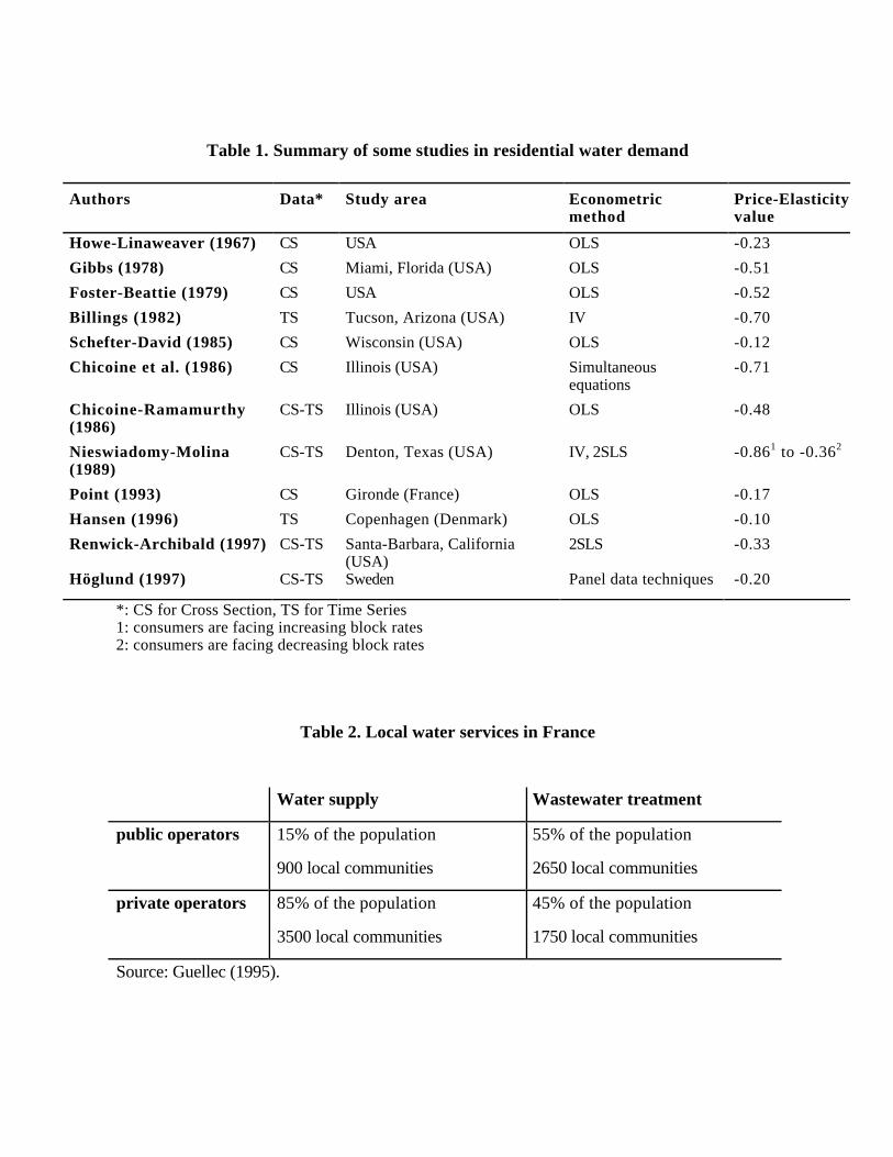
Table 1. Summary of some studies in residential water demand

Authors Data* Study area Econometricmethod

Price-Elasticityvalue

Howe-Linaweaver (1967) CS USA OLS -0.23

Gibbs (1978) CS Miami, Florida (USA) OLS -0.51

Foster-Beattie (1979) CS USA OLS -0.52

Billings (1982) TS Tucson, Arizona (USA) IV -0.70

Schefter-David (1985) CS Wisconsin (USA) OLS -0.12

Chicoine et al. (1986) CS Illinois (USA) Simultaneousequations

-0.71

Chicoine-Ramamurthy(1986)

CS-TS Illinois (USA) OLS -0.48

Nieswiadomy-Molina(1989)

CS-TS Denton, Texas (USA) IV, 2SLS -0.861 to -0.362

Point (1993) CS Gironde (France) OLS -0.17

Hansen (1996) TS Copenhagen (Denmark) OLS -0.10

Renwick-Archibald (1997) CS-TS Santa-Barbara, California(USA)

2SLS -0.33

Höglund (1997) CS-TS Sweden Panel data techniques -0.20

*: CS for Cross Section, TS for Time Series1: consumers are facing increasing block rates2: consumers are facing decreasing block rates

Table 2. Local water services in France

Water supply Wastewater treatment

public operators 15% of the population

900 local communities

55% of the population

2650 local communities

private operators 85% of the population

3500 local communities

45% of the population

1750 local communities

Source: Guellec (1995).

Table 3. Descriptive statistics for variables in the sample

Variable Type Mean StandardDeviatio

n

Minimum Maximum

Y CS-TS 152.68 40.43 76.00 334.00AP CS-TS 8.95 3.37 3.34 20.66MP CS-TS 8.00 3.32 3.09 19.48DEN CS 265.87 490.65 8.69 3 818.33AGE60 CS 18.51 5.53 6.60 48.57HH CS 42.96 8.55 25.45 66.67ACT CS 90.64 4.14 76.38 100.00HOU CS 75.11 17.03 10.10 100.00BATH CS 82.94 10.92 26.67 96.22CAR CS 81.31 7.13 62.16 96.21H49 CS 38.87 20.24 2.32 88.46H82 CS 13.21 7.45 1.00 39.31I CS-TS 106 797.44 16 325.22 63007.00 180 533.00RAIN CS-TS 183.97 46.68 108.00 299.70TOTRAIN CS-TS 774.21 112.41 474.10 1 087.50CO CS-TS 5 106.00 5 515.00 78.00 15 907.00LEA CS-TS 273.00 285.00 2.00 908.00NET CS-TS 197.00 184.00 2.00 511.00

with Y, average annual consumption of residential water (cubic meter/subscriber) ;AP, average price of residential water defined as total bill divided by total consumption (FF/cubicmeter) ;MP, marginal price of water defined as the price of the last unit of consumption (FF/cubic meter) ;DEN, population density (number of inhabitants/square kilometer) ;AGE60, proportion of inhabitants aged more than sixty in the whole population of the community ;HH, proportion of households composed of one or two members ;ACT, industrial activity rate ;HOU, proportion of private housings in the population of the community homes ;BATH, proportion of homes equipped with a bath ;CAR, proportion of homes of which the occupant owns one or more car ;H49, proportion of housings built before 1949 in the total population of housings (including occasionalhousings, second homes, and vacant housings);H82, proportion of housings built after 1982 in the total population of housings (including occasionalhousings, second homes, and vacant housings);I, average taxable income (FF/taxable household) ;RAIN, total amount of rainfall measured in June, July and August ;TOTRAIN, total amount of rainfall measured in year t ;CO, number of service connections;LEA, number of leaks detected ;NET, size of the water system (kilometers of mainlines).

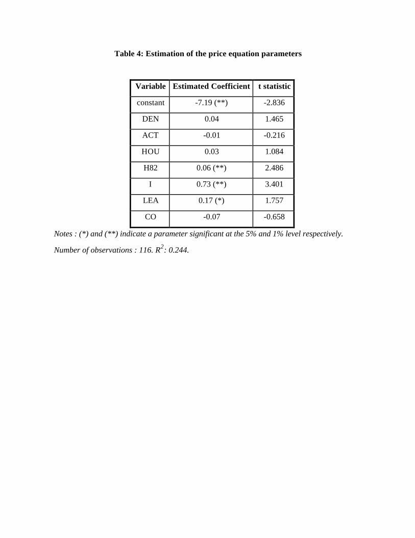
Table 4: Estimation of the price equation parameters

Variable Estimated Coefficient t statistic

constant -7.19 (**) -2.836

DEN 0.04 1.465

ACT -0.01 -0.216

HOU 0.03 1.084

H82 0.06 (**) 2.486

I 0.73 (**) 3.401

LEA 0.17 (*) 1.757

CO -0.07 -0.658

Notes : (*) and (**) indicate a parameter significant at the 5% and 1% level respectively.

Number of observations : 116. R2: 0.244.

TABLE 5. MODEL WITH DECOMPOSED PRICE VARIABLE

Test Degrees offreedom

Test statistic P-value

Within / Within+instruments 4 3.550 0.470

Within / GLS 4 61.879 1.2e-012

Within / HT 2 3.964 0.138

HT / AM 4 5.129 0.274

AM / BMS 4 2.552 0.635

OLS Within GLS BMSconstant -4.883(**)

(-4.666)... -0.481

(-1.465)-0.458

(-1.394)

MP -0.158(**)(-7.653)

-0.019(-0.818)

-0.086(**)(-4.838)

-0.072(**)(-3.550)

AP-MP -0.172(**)(-12.067)

-0.265(**)(-11.350)

-0.210(**)(-13.082)

-0.216(**)(-10.796)

I 0.472(**)(8.803)

0.024(0.574)

0.123(**)(3.333)

0.109(**)(2.885)

RAIN 0.024(0.892)

-0.007(-0.755)

-0.010(-1.038)

-0.008(-0.907)

DEN -0.000(-0.892)

... -2.4e-005(-0.148)

-1.6e-005(-0.099)

AGE60 -0.102(*)(-2.388)

... -0.169(*)(-2.543)

-0.171(**)(-2.577)

HH 0.043(0.686)

... 0.160(1.660)

0.164(1.696)

ACT 0.833(**)(3.787)

... 1.039(**)(2.999)

1.051(**)(3.031)

HOUSE -0.239(**)(-8.105)

... -0.207(**)(-4.504)

-0.203(**)(-4.364)

BATH 0.099(1.492)

... 0.072(0.697)

0.060(0.585)

CAR 0.394(*)(2.571)

... 0.464(*)(1.928)

0.462(1.916)

H49 0.060(**)(4.115)

... 0.057(**)(2.596)

0.058(**)(2.614)

H82 -0.170(**)(-11.220)

... -0.176(**)(-7.468)

-0.178(**)(-7.459)

t statistics are in parentheses ; significance at the 5% and 1% level denoted by (*) and (**)respectively ; ... : not identifiable.

TABLE 6. AVERAGE PRICE MODEL

Test Degrees offreedom

Test statistic P-value

Within /Within+instruments

3 2.219 0.528

Within / GLS 3 17.497 5.6e-4

Within / HT 1 1.302 0.254

HT / AM 4 2.544 0.637

AM / BMS 4 2.971 0.563

OLS Within GLS BMSconstant -5.786(**)

(-5.119)... -0.487

(-1.357)-2.740(**)

(-3.216)

AP -0.244(**)(-10.007)

-0.205(**)(-9.858)

-0.217(**)(-11.143)

-0.215(**)(-10.605)

I 0.491(**)(8.438)

0.061(1.344)

0.106(*)(2.489)

0.092(*)(2.104)

RAIN 0.010(0.355)

-0.017(-1.675)

-0.017(-1.688)

-0.017(-1.688)

DEN -0.000(-0.812)

... -3.7e-005(-0.149)

-2.2e-005(-0.086)

AGE60 -0.065(-1.412)

... -0.135(-1.323)

-0.222(*)(-2.089)

HH 0.005(0.078)

... 0.133(0.897)

0.063(0.421)

ACT 0.835(**)(3.498)

... 1.047(*)(1.961)

6.219(**)(3.357)

HOU -0.310(**)(-10.011)

... -0.302(**)(-4.334)

-0.436(**)(-5.223)

BATH 0.180(*)(2.535)

... 0.209(1.331)

0.589(**)(2.886)

CAR 0.568(**)(3.435)

... 0.705(1.908)

-1.233(-1.622)

H49 0.088(**)(5.600)

... 0.086(*)(2.567)

0.036(0.953)

H82 -0.126(**)(-7.960)

... -0.117(**)(-3.297)

-0.119(**)(-3.349)

t statistics are in parentheses ; significance at the 5% and 1% level denoted by * and (**)respectively ; ... : not identifiable.

iTo be presented at the EAERE annual meeting in Venice, June 1998. Part of this paper was

written while the second author was visiting University of Wisconsin-Madison. We thank O.

Alexandre (Cemagref Strasbourg), M. Muller (CGE Région Est) for the data used in the paper,

R. Boumahdi and M. Moreaux for helpful comments. All remaining errors are ours.

iiE.R.N.A.-I.N.R.A., Université des Sciences Sociales de Toulouse, 21 Allée de Brienne, 31000

Toulouse, France. Email: cnauges@toulouse.inra.fr, thomas@toulouse.inra.fr

iii The 1992 Water Act also prohibits a lump sum fee to be charged to residential consumers.