Priority Algorithms for the Subset-Sum Problemy3ye/publications/msc-thesis.pdfPriority Algorithms...
68
Priority Algorithms for the Subset-Sum Problem by Yuli Ye A thesis submitted in conformity with the requirements for the degree of Master of Science Graduate Department of Computer Science University of Toronto Copyright c 2006 by Yuli Ye
Transcript of Priority Algorithms for the Subset-Sum Problemy3ye/publications/msc-thesis.pdfPriority Algorithms...

Priority Algorithms for the Subset-Sum Problem
by
Yuli Ye
A thesis submitted in conformity with the requirements
for the degree of Master of Science
Graduate Department of Computer Science
University of Toronto
Copyright c© 2006 by Yuli Ye

Abstract
Priority Algorithms for the Subset-Sum Problem
Yuli Ye
Master of Science
Graduate Department of Computer Science
University of Toronto
2006
Priority algorithms capture the key notion of “greediness” in the sense that they process the
“best” data item one at a time, depending on the current knowledge of the input, while keeping
a feasible solution for the output. Although priority algorithms are often simple to state,
their relative power is not completely understood. In this thesis, we study priority algorithms
for the Subset-Sum Problem. In particular, several variants of priority algorithms: revocable
versus irrevocable, fixed versus adaptive, non-increasing order versus non-decreasing order; are
analyzed and corresponding lower bounds are provided.
ii

Dedication
Dedicate to my beloved parents Lvan Ye and Yi Jin
iii

Acknowledgements
First of all, I would like to thank Allan Borodin, my supervisor, for introducing to me this
wonderful topic, and the numerous discussions and encouragements he gave me during the
study of my master’s degree. I also thank him for the approximation algorithms course he
taught in the winter of 2005, which has become an inspiration for this work. Very special
thanks go to John Brzozowski for bringing me into the world of scientific research and giving
me invaluable help during the very early stage of my research. I thank him for the four years of
collaboration and friendship, and the two papers we wrote together; without him, I would miss
a great deal of my life. I also thank Avner Magen for carefully reading my thesis and many
comments and suggestions to make it better.
I am greatly indebted to my parents for their long-time financial and emotional support,
and my family and friends at Waterloo and Toronto; without them, this thesis would become
impossible.
The financial support from the Natural Sciences and Engineering Research Council of
Canada and the Department of Computer Science, University of Toronto are gratefully ac-
knowledged.
iv

Contents
1 Introduction 1
1.1 Subset-Sum Problem . . . . . . . . . . . . . . . . . . . . . . . . . . . . . . . . . . 1
1.2 Priority Model and Related Work . . . . . . . . . . . . . . . . . . . . . . . . . . . 3
1.3 Motivations . . . . . . . . . . . . . . . . . . . . . . . . . . . . . . . . . . . . . . . 4
2 Preliminaries 6
2.1 Notation and Definitions . . . . . . . . . . . . . . . . . . . . . . . . . . . . . . . . 6
2.1.1 Definition of the Subset-Sum Problem . . . . . . . . . . . . . . . . . . . . 7
2.1.2 Priority Model . . . . . . . . . . . . . . . . . . . . . . . . . . . . . . . . . 8
2.2 Adversarial Strategy . . . . . . . . . . . . . . . . . . . . . . . . . . . . . . . . . . 10
2.2.1 An Example . . . . . . . . . . . . . . . . . . . . . . . . . . . . . . . . . . 11
3 Irrevocable Priority Algorithms 12
3.1 General Simplifications . . . . . . . . . . . . . . . . . . . . . . . . . . . . . . . . . 12
3.1.1 Implicit Terminal Conditions . . . . . . . . . . . . . . . . . . . . . . . . . 12
3.1.2 Exclusion of Small and Extra Large Data Items . . . . . . . . . . . . . . . 14
3.2 Fixed Irrevocable Priority Algorithms . . . . . . . . . . . . . . . . . . . . . . . . 17
3.2.1 Description of the Algorithm . . . . . . . . . . . . . . . . . . . . . . . . . 18
3.2.2 Proof of the Upper Bound . . . . . . . . . . . . . . . . . . . . . . . . . . . 19
3.3 Adaptive Irrevocable Priority Algorithms . . . . . . . . . . . . . . . . . . . . . . 20
v

3.3.1 Deriving the Lower Bound . . . . . . . . . . . . . . . . . . . . . . . . . . . 20
4 Revocable Priority Algorithms 22
4.1 More Simplifications . . . . . . . . . . . . . . . . . . . . . . . . . . . . . . . . . . 22
4.1.1 Two Assumptions . . . . . . . . . . . . . . . . . . . . . . . . . . . . . . . 22
4.1.2 Four Operational Modes . . . . . . . . . . . . . . . . . . . . . . . . . . . . 23
4.2 Fixed Revocable Priority Algorithms . . . . . . . . . . . . . . . . . . . . . . . . . 24
4.2.1 Non-Increasing Order . . . . . . . . . . . . . . . . . . . . . . . . . . . . . 24
4.2.2 Non-Decreasing Order . . . . . . . . . . . . . . . . . . . . . . . . . . . . . 28
4.2.3 A General Lower Bound . . . . . . . . . . . . . . . . . . . . . . . . . . . . 37
4.3 Adaptive Revocable Priority Algorithms . . . . . . . . . . . . . . . . . . . . . . . 41
4.3.1 Deriving a Lower Bound . . . . . . . . . . . . . . . . . . . . . . . . . . . . 41
4.3.2 A Better Algorithm . . . . . . . . . . . . . . . . . . . . . . . . . . . . . . 43
5 Conclusion 55
5.1 Summary of Results . . . . . . . . . . . . . . . . . . . . . . . . . . . . . . . . . . 55
5.2 Questions and Future Directions . . . . . . . . . . . . . . . . . . . . . . . . . . . 56
Bibliography 58
vi

List of Tables
4.1 Corresponding symbols. . . . . . . . . . . . . . . . . . . . . . . . . . . . . . . . . 43
5.1 Summary of results. . . . . . . . . . . . . . . . . . . . . . . . . . . . . . . . . . . 56
5.2 Corresponding values. . . . . . . . . . . . . . . . . . . . . . . . . . . . . . . . . . 56
vii

List of Figures
2.1 An example of an adversarial strategy. . . . . . . . . . . . . . . . . . . . . . . . . 11
3.1 Classification for the fixed irrevocable priority algorithm. . . . . . . . . . . . . . 18
4.1 Adversarial strategy for fixed non-increasing order. . . . . . . . . . . . . . . . . . 25
4.2 Classification for non-increasing order. . . . . . . . . . . . . . . . . . . . . . . . . 26
4.3 Adversarial strategy for fixed non-decreasing order. . . . . . . . . . . . . . . . . . 29
4.4 Classification for non-decreasing order. . . . . . . . . . . . . . . . . . . . . . . . . 30
4.5 Stack with one data item. . . . . . . . . . . . . . . . . . . . . . . . . . . . . . . . 32
4.6 Stack with two data items. . . . . . . . . . . . . . . . . . . . . . . . . . . . . . . 32
4.7 Adversarial strategy for rank(u2) > rank(u1). . . . . . . . . . . . . . . . . . . . . 38
4.8 Adversarial strategy for rank(u3) > rank(u2). . . . . . . . . . . . . . . . . . . . . 39
4.9 Adversarial strategy for rank(u4) > rank(u3). . . . . . . . . . . . . . . . . . . . . 39
4.10 Adversarial strategy for rank(u1) > rank(u2) > rank(u3) > rank(u4). . . . . . . 40
4.11 Adversarial strategy for adaptive revocable priority algorithms. . . . . . . . . . . 42
4.12 Classification for the adaptive revocable priority algorithm. . . . . . . . . . . . . 43
viii

Chapter 1
Introduction
This chapter introduces two main objects of the thesis: the Subset-Sum Problem and the
Priority Model. A list of previous work done in related fields is surveyed and some motivations
for this topic are provided.
1.1 Subset-Sum Problem
The Subset-Sum Problem (SSP) is one the most fundamental NP-complete problems [11], and
perhaps the simplest of its kind. Given a set of n data items with positive weights and a capacity
c, the decision version of SSP asks whether there exists a subset whose corresponding total
weight is exactly the capacity c; the maximization version of SSP is to find a subset such that
the corresponding total weight is maximized without exceeding the capacity c. The Subset-Sum
Problem has many applications; for example, a decision version of SSP with unique solutions
represents a secret message in a SSP-based cryptosystem. It also appears in more complicated
combinatorial problems [25], scheduling problems [15, 16], 0-1 integer programs [9, 10], and bin
packing algorithms [6, 7]. The Subset-Sum Problem is often thought of as a special case of
the Knapsack Problem, where the weight of a data item is proportional to its size. Therefore,
algorithms for the Knapsack Problem can be applied for SSP automatically. However, as simple
1
Chapter 1. Introduction 2
as it is, the Subset-Sum Problem has a better structure and hence sometimes admits better
algorithms.
A naive algorithm with time complexity O(n2n) solves SSP, by iterating through all possible
subsets, and for each subset comparing its sum with the capacity c. A better algorithm is
proposed in 1974 using the Horowitz and Sahni decomposition scheme, which achieves time
O(n2n
2 ); exact algorithms for solving SSP have not been improved since then. From a practical
point of view, if the capacity c is relatively small, there exist dynamic programming algorithms
that can run much faster. A classic pseudo-polynomial algorithm using Bellman recursion
solves SSP in both time and space O(nc), and many other algorithms have been proposed
under different heuristics, see [21] for a detailed comparison.
Approximation algorithms have also been studied extensively for SSP. The first FPTAS
is due to Ibarra and Kim [18], which has time and space complexity O( nε2 ) and O(n + 1
ε3 )
respectively. This is subsequently improved by Lawler [22], Gens and Levner [12, 13, 14]. The
best known approximation algorithm is due to Kellerer et al. [20], and has time and space
complexity O(min{nε, n + 1
ε2 log 1ε}) and O(n + 1
ε) respectively. The idea of the algorithm is
as follows. The algorithm first separates data items into small items, data items with weight
≤ εc, and large items. It can be easily seen that any (1 − ε)-approximation algorithm for the
large items remains an (1 − ε)-approximation algorithm for the whole set if we fill the small
items during the end of the algorithm in a greedy way. Next, it partitions the interval [εc, c]
into subintervals of equal length εc. For each of such intervals, the algorithm selects a constant
number of candidates; these data items form the set of relevant items. The paper then proves
that the optimal solution on the set of relevant items approximates the optimal solution on the
whole set with accuracy εc. Finally, the algorithm computes the optimal solution on the set
of relevant items using relaxed dynamic programming; divide-and-conquer and backtracking
techniques are applied to secure the bounds on running time and required space.
In terms of “greedy” approximation algorithms, not much work has been done. The first such
Chapter 1. Introduction 3
algorithm is derived directly from a “greedy” algorithm of the Knapsack Problem [24], which
considers the data item with maximum weight alone as a possible alternative solution, while
processing the rest of the data items greedily to build the other solution. It is not hard to see
that this strategy guarantees an approximation ratio 12. An alternative greedy algorithm [24],
and maybe the most intuitive one, considers data items in non-increasing order, and accepts
one if it fits. This algorithm has a better average result, but the worst case approximation
ratio still remains at 12. However, by applying it n times on item sets {1, . . . , n}, {2, . . . , n},
{3, . . . , n}, and so on, respectively, Martello and Toth [23] prove that the approximation ratio
can be improved to 34. Of course, the disadvantages of this approach are that it requires n passes
and needs to maintain n solutions. In [19], Iwama and Taketomi manage to show that a better
strategy exists for one-pass algorithms even if the ordering of data items is arbitrary. They prove
a tight bound on the approximation ratio of√
5−1
2≈ 0.618 for online revocable algorithms of
SSP. These four algorithms represent the current stage of “greedy” approximation algorithms,
yet not all of them fit in our definition of priority algorithms. The second and the fourth are
most relevant to this thesis; the second is an irrevocable priority algorithm and the fourth is
an online revocable algorithm which is a special case of revocable priority algorithms. The
remaining two are not so relevant as they belong to a more general class of BT algorithms
defined in [1].
1.2 Priority Model and Related Work
Greedy algorithms are among the most natural attempts in solving combinatorial optimization
problems. Although they seldom yield optimal solutions for hard problems, like the class of NP-
hard problems, they sometimes give good approximation ratios; for example, a simple greedy
algorithm yields the best known constant approximation ratio of 2 for the vertex cover problem.
The Priority Model [5], recently established by Borodin et al., formulates a notion of “greed-
iness”. This formulation provides us a tool to assess the computational power and limitation

Chapter 1. Introduction 4
for greedy algorithms, especially in terms of their approximability. The key characteristics
of priority algorithms are that it has an ordering function evaluating the priority of each data
item, processes data items in turn according to their priorities and builds the solution incremen-
tally. For this reason, priority algorithms can be viewed as an extension of online algorithms,
where the ordering function instead of nature decides which data item comes next. The algo-
rithms defined under this framework are usually efficient; running times are often bounded by
O(n log n)1.
In addition to [5], where priority algorithms for scheduling problems are studied, several
papers have been published along this line, analyzing the relative power of priority algorithms
on many problems, including facility location, set cover [2], interval selection [17], and various
graph problems [4, 8]. Results have shown that non-trivial lower bounds for such models
exist for many NP-hard problems, and some gaps with respect to the approximation ratio are
inherently difficult to close.
1.3 Motivations
The main motivation of this work comes from two papers. The first one is by Iwama and
Taketomi [19], where a tight bound on the approximation ratio of√
5−1
2≈ 0.618 has been
proved for online revocable algorithms for SSP. Since priority algorithms are natural extensions
of online algorithms, it is interesting to see whether the additional power of priority algorithms
improves the approximation ratio. The second one is the master thesis work done by Horn [17],
which extends the work from the scheduling approximation paper by Bar-Noy et al. [3]. In
her thesis, one-pass algorithms with revocable acceptances are explicitly studied for the job
interval selection problem. Both of these two papers mentioned above are built on an important
feature that we are allowed to make revocable decisions on accepted items. This new feature
brings us more power, and provides a new prospective for priority algorithms. Furthermore,
1Note that we do not insist upon any time complexity on the model, it is determined by the actual algorithm.

Chapter 1. Introduction 5
as a fundamental NP-complete problem, the Subset-Sum Problem has a very simple structure.
Therefore, studying priority algorithms for SSP gives us some additional benefits:
• Lower bounds on approximation ratio of priority algorithms for SSP provide us some
insights into how well priority algorithms can approximate for more complicated problems.
For example, a lower bound for SSP automatically implies a lower bound for the Knapsack
Problem.
• Approximability gaps are of fundamental interest to the theoretical computer science com-
munity, exhibiting such gaps for relative simple structures may reveal some of mysteries
as to why those gaps are hard to close.
Nevertheless, priority algorithms for SSP themselves are interesting enough as they have never
been studied, and their behavior can give us more evidence of how good greedy algorithms can
be.
The rest of the thesis is organized as follows. In Chapter 2, we give formal definitions for the
Subset-Sum Problem, the Priority Model and the adversarial strategy. We deal with irrevocable
and revocable priority algorithms for SSP in Chapter 3 and 4 respectively. In Chapter 5, we
conclude our work and discuss future directions.
Chapter 2
Preliminaries
In this chapter, we formally define the Subset-Sum Problem and the Priority Model. We also
describe the adversarial strategy, which is the tool for deriving lower bounds.
2.1 Notation and Definitions
Since the basic elements of SSP are data items, we first define some of notation used for data
items and sets of data items. We use bold font letters to denote sets of data items. For a
give set R of data items, we use |R| to denote its size, i.e., the number of data items in R;
and use ‖R‖ to denote the corresponding total weight. For a data item u, we sometimes use
u to represent the singleton set {u}, and 2u to represent the multi-set {u, u}; we also use u to
represent its weight since it is the only attribute. The term u here is an overloaded term, but
the meaning will become clear in the actual context. For set operations, the standard notation
for set addition and set subtraction are ∪ and \ respectively. In this thesis, we use ⊕ to denote
set addition, and use ⊖ to denote set subtraction, as they deliver more intuitive meaning of
adding and deleting data items. We keep the traditional ∩ to denote set intersection.
6

Chapter 2. Preliminaries 7
2.1.1 Definition of the Subset-Sum Problem
We provide a slightly different definition from the one in Section 1.1 for the suit of our analysis.
Here, we make two additional assumptions. First of all, the weights are all scaled to their
relative values to the capacity; hence we can use 1 instead of c for the capacity. Secondly, we
assume each data item has weight less than or equal to 1, for otherwise the weight of that data
item exceeds the capacity, hence useless to our solution. Therefore, an instance σ of SSP is
a set I = {u1, u2, . . . , un} of n data items with ui ∈ (0, 1] for all i ∈ [1, n]. The set I is the
input set, and u1, u2, . . . , un are the data items. A feasible solution of σ is a subset B of I such
that ‖B‖ ≤ 1. An optimal solution of σ is a feasible solution with maximum weight. We can
formulate SSP as a solution of the following integer programming:
maximize
n∑
i=1
uixi (2.1)
subject ton∑
i=1
uixi ≤ 1, (2.2)
where xi ∈ {0, 1} and i ∈ [1, n]. Let A be an algorithm for SSP, for a given instance σ, we denote
A(σ) the solution achieved by A and OPT(σ), the optimal solution, then the approximation ratio
of A on σ is denoted by
ρ(A, σ) =‖A(σ)‖
‖OPT(σ)‖.
Let Σ be the set of all instances of SSP, then the approximation ratio of A over Σ is denoted by
ρ(A) = infσ∈Σ
ρ(A, σ).
In a particular analysis, the algorithm and the problem instance are usually fixed. For conve-
nience, we often use ALG, OPT and ρ to denote the algorithm’s solution, the optimal solution
and the approximation ratio respectively.

Chapter 2. Preliminaries 8
2.1.2 Priority Model
We base our terminology and model on that of [5], and start with the class of fixed order
irrevocable priority algorithms for SSP. For a given instance σ, a fixed (order) irrevocable priority
algorithm maintains a feasible solution B throughout the algorithm. At each step, it looks at
a data item with the highest priority in I according to some pre-determined ordering, then it
can either discard it, i.e., remove it from I without doing anything, or add it to B, i.e., move it
from I to B. The structure of a fixed irrevocable priority algorithm is described as follows:
Fixed Irrevocable Priority
Ordering: Determine, without looking at I, a total ordering of all possible data items
while I is not empty
next := index of the data item in I that comes first in the ordering
Decision: Decide whether or not to add unext to B, and then remove unext from I
end while
An adaptive (order) irrevocable priority algorithm is similar to a fixed one, but instead of looking
at a data item according to some pre-determined ordering, the algorithm is allowed to reorder
the remaining data items in I at each step. This gives the algorithm an advantage since now it
can take into account the information that has been revealed so far to determine which is the
best data item to consider next. The structure of an adaptive irrevocable priority algorithm is
described as follows:
Adaptive Irrevocable Priority
while I is not empty
Ordering: Determine, without looking at I, a total ordering of all possible data items
next := index of the data item in I that comes first in the ordering
Decision: Decide whether or not to add unext to B, and then remove unext from I
end while
Chapter 2. Preliminaries 9
The above defined priority algorithms are “irrevocable” in the sense that once a data item
is admitted to the solution it cannot be removed. We can extend our notion of “fixed” and
“adaptive” to the class of revocable priority algorithms, where revocable decisions on accepted
data items are allowed. Accordingly, those algorithms are called fixed (order) revocable and
adaptive (order) revocable priority algorithms respectively; they are formally defined as follows:
Fixed Revocable Priority
Ordering: Determine, without looking at I, a total ordering of all possible data items
while I is not empty
next := index of the data item in I that comes first in the ordering
Decision: Decide whether or not to add unext to B by discarding any number data items
in B, and then remove unext from I
end while
Adaptive Revocable Priority
while I is not empty
Ordering: Determine, without looking at I, a total ordering of all possible data items
next := index of the data item in I that comes first in the ordering
Decision: Decide whether or not to add unext to B by discarding any number data items
in B, and then remove unext from I
end while
The extension1 to revocable acceptances does give us some additional power, for example, as
shown in [19], for the online version of SSP, irrevocable algorithms do not achieve any constant
bound approximation ratio, while revocable algorithms achieve a tight approximation ratio√
5−1
2≈ 0.618.
1This extension applies to priority algorithms for packing problems.
Chapter 2. Preliminaries 10
2.2 Adversarial Strategy
We often utilize an adversary in proving lower bounds. For a given priority algorithm, we run
the adversary against the algorithm in the following scheme. At the beginning of the algorithm,
the adversary first presents a set of data items to the algorithm, possibly with some data items
having the same weight. Furthermore, our adversary promises that the actual input is contained
in this set2. Note that weight is the only criterion for which the algorithm can compare two
data items, hence the algorithm cannot distinguish two data items if they have the same weight.
At each step, the adversary asks the algorithm to select one data item in the remaining set and
make a decision on that data item. Once the algorithm makes a decision on the selected item,
the adversary then has the power to remove any number of data items in the remaining set;
this repeats until the remaining set is empty, which leads to the end of the algorithm.
For convenience, we often use a diagram to illustrate an adversarial strategy. A diagram
of an adversarial strategy is an acyclic directed graph, where each node represents a possible
state of the strategy, and each arc indicates a possible transition. Each state of the strategy
contains two boxes. The first box indicates the current solution maintained by the algorithm,
the second box indicates the remaining set of data items maintained by the adversary. A state
can be either terminal or non-terminal. A state is terminal if and only if it is a sink, in the sense
that the adversary no longer need perform any additional action; we indicate a terminal state
using bold boxes. Each transition also contains two lines of actions. The first line indicates the
action taken by the algorithm and the second line indicates the action taken by the adversary;
we use ⊘ to indicate no action. Note that to calculate a lower bound for the approximation ratio
of an algorithm, it is sufficient to consider the approximation ratios achieved in all terminal
states. An example is given in the next subsection.
2This assumption is optional. The lower bounds clearly hold for a stronger adversary.

Chapter 2. Preliminaries 11
2.2.1 An Example
Let us take a fixed revocable priority algorithm which orders data item u1 = 0.8 before u2 = 0.5
as an example; see Fig. 2.1.
⊕u1
⊘
n1 : n2 :u1 2u2 u1 2u2
⊕u2,⊖u1
⊖u2
u2u2s1 : u1s2 :
⊕u2,⊖u2⊘
Figure 2.1: An example of an adversarial strategy.
At the beginning, the adversary presents one copy of u1 and two copies of u2 to the algorithm;
this state is represented by the state n1. Since the algorithm orders u1 before u2, it selects u1;
this is indicated by the first line under the transition from n1 to n2. Accordingly, adversary
takes no action; this is indicated by the second line under the transition from n1 to n2. The first
transition leads to the state n2, where u1 is in the algorithm’s solution while the adversary still
holds two copies of u2 for the remaining input. There are two choices for the algorithm starting
from n2. The first one is indicated by the transition from n2 to s1, where the algorithm takes
u2 into the solution and discards the previously accepted u1. If this is the case, the adversary
deletes u2 from the remaining input. The second one is indicated by the transition from n2
to s2, where the algorithm just discards u2. If this is the case, the adversary takes no action.
Both s1 and s2 are terminal states since no further action is required for the adversary. If the
algorithm terminates in state s1, it has approximation ratio 58. If the algorithm terminates in
state s2, it has approximation ratio 0.8. Since they are the only terminal states, the algorithm
cannot achieve approximation ratio better than 5
8.

Chapter 3
Irrevocable Priority Algorithms
Let α1 ≈ 0.657 be the real root of the equation
2x3 + x2 − 1 = 0 (3.1)
between 0 and 1. In this chapter, we prove a tight bound of α1 on the approximation ratio of
irrevocable priority algorithms for SSP. It is interesting that there is no approximability gap
between fixed and adaptive irrevocable priority algorithms. Before we get into the proof, we
first provide two simplifications for general priority algorithms.
3.1 General Simplifications
The two simplifications given in this section are both based on the approximation ratio, say α,
we want to achieve.
3.1.1 Implicit Terminal Conditions
Since we are interested in approximation algorithms, we can terminate an algorithm at any
time if the approximation ratio of α is achieved. This condition is called a terminal condition.
12

Chapter 3. Irrevocable Priority Algorithms 13
• For a fixed irrevocable priority algorithm, the terminal condition is satisfied, if at the
beginning of some step of the algorithm, u is the next data item to be examined, B′ =
(B ⊕ u) and α ≤ ‖B′‖ ≤ 1.
• For an adaptive irrevocable priority algorithm, the terminal condition is satisfied, if at
the beginning of some step of the algorithm, there exists some u ∈ I and B′ = (B ⊕ u)
such that α ≤ ‖B′‖ ≤ 1. In this case, u is the next data item, and the approximation
ratio can be achieved.
• For a fixed revocable priority algorithm, the terminal condition is satisfied, if at the
beginning of some step of the algorithm, u is the next data item to be examined, and
there exists B′ ⊆ (B ⊕ u) such that α ≤ ‖B′‖ ≤ 1.
• For an adaptive revocable priority algorithm, the terminal condition is satisfied, if at the
beginning of some step of the algorithm, there exists some u ∈ I and B′ ⊆ (B ⊕ u) such
that α ≤ ‖B′‖ ≤ 1. In this case, u is the next data item, and the approximation ratio
can be achieved.
It is clear that in all four cases, the algorithm can take B′ as the final solution and immediately
terminate. For any algorithm given in this thesis, we will not explicitly state the check of the
terminal condition; we assume that the algorithm tests the condition whenever it considers
the next data item, and will terminate if the condition is satisfied. Note that here we do not
impose any time bound for checking the terminal condition in the general model. But for all the
algorithms studied in this thesis, the extra check for the terminal condition does not increase
much for the time complexity as the input against such test is highly restricted, and the running
time is bounded by a constant.
Chapter 3. Irrevocable Priority Algorithms 14
3.1.2 Exclusion of Small and Extra Large Data Items
For the approximation ratio α, a data item u is said to be in class S and X if 0 < u ≤ 1 − α
and α ≤ u ≤ 1 respectively. A data item is small if it is in S, and extra large if it is in X; a
data item is relevant if it is neither small nor extra large. Let Σ′ be the set of instances of SSP
whose input contains only relevant data items, and let A′ be a priority algorithm over Σ′; we
call A′ a restricted algorithm. For a given instance σ ∈ Σ with input I, we let σ′ ∈ Σ′ be the
instance with input I⊖S⊖X. An algorithm A over Σ is a completion1 of A′ if for any instance
σ, either ρ(A, σ) ≥ α or X ∩ I = ∅, A(σ) ⊖ S = A′(σ′) and A(σ) ∩ S = S ∩ I. This definition
implies that if X ∩ I 6= ∅, then we have ρ(A, σ) ≥ α.
Proposition 3.1.1 Let A be a completion of A′. If A′ achieves approximation ratio α over
Σ′, then A achieves approximation ratio α over Σ.
Proof: Suppose that A′ achieves approximation ratio α over Σ′, but A achieves approximation
ratio less than α over Σ, then X ∩ I = ∅ and for a given instance σ, A(σ) ⊖ S = A′(σ′) and
A(σ) ∩ S = S ∩ I. Hence, we have
‖OPT(σ) ∩ S‖ ≤ ‖S ∩ I‖ = ‖A(σ) ∩ S‖.
Therefore, approximation ratio of A on σ is given by
ρ(A, σ) =‖A(σ)‖
‖OPT(σ)‖=
‖A(σ) ∩ S‖ + ‖A(σ) ⊖ S‖
‖OPT(σ) ∩ S‖ + ‖OPT(σ) ⊖ S‖≥
‖A(σ) ⊖ S‖
‖OPT(σ) ⊖ S‖.
On the other hand, since the algorithm A′ achieves approximation ratio of α on σ′, we have
ρ(A′, σ′) =‖A′(σ′)‖
‖OPT(σ′)‖≥ α.
Since A′(σ′) = A(σ) ⊖ S, and ‖OPT(σ′)‖ ≥ ‖OPT(σ) ⊖ S‖. Therefore,
ρ(A, σ) ≥‖A(σ) ⊖ S‖
‖OPT(σ) ⊖ S‖≥
‖A′(σ′)‖
‖OPT(σ′)‖≥ α.
Therefore, the algorithm A achieves approximation ratio of α, which is a contradiction.
1This is only defined on valid algorithms, i.e., both solutions of A and A′ have to be feasible.

Chapter 3. Irrevocable Priority Algorithms 15
Proposition 3.1.1 shows that if we have a restricted algorithm which achieves approximation
ratio α over Σ′ and it has a completion, then the completion achieves approximation ratio α
over Σ. This gives us some hope, yet it is not enough to exclude small and extra large data
items for the following two reasons:
• We still do not know how to construct a completion from a restricted algorithm for specific
class of priority algorithms.
• Such construction may alter the class of the original algorithm, hence may not be appli-
cable.
Therefore, we need the following definition. For a given class C of priority algorithms, a
completion is C-preserving if both algorithms are in C. Now the remaining task is to show for a
specific class C, how to construct a C-preserving completion from a restricted algorithm. Note
that for most classes of algorithms studied in this thesis, we do not impose any ordering to
process data items. That means for those classes, one has the freedom to design an algorithm
to process data items in any order. There are two exceptions: the non-increasing and non-
decreasing order revocable priority algorithms studied in Section 4.2, each of them imposes a
restricted ordering, hence we have to deal them separately.
Proposition 3.1.2 Let C be the class of [ fixed | adaptive ] [ irrevocable | revocable ] priority
algorithms, then there exists a C-preserving completion from a restricted algorithm in C.
Proof: Given a restricted algorithm A′ in C, the algorithm A is constructed from A′ with
three phases:
• Phase 1: if there is an extra large data item then take that data item as the final solution,
and terminate the algorithm; otherwise go to Phase 2.
• Phase 2: run the algorithm A′ on σ′, and then go to Phase 3.
Chapter 3. Irrevocable Priority Algorithms 16
• Phase 3: greedily fill the solution with small data items until either an overflow or the
exhaustion of small data items; terminate the algorithm.
It is clear that the above construction preserves the class of fixed irrevocable priority algorithms,
which is the most restricted class among the four combinations. Therefore, such construction
is C-preserving. There are three possible ways for algorithm A to terminate. If the algorithm
A terminates in Phase 1, then it clearly achieves approximation ratio of α; otherwise, it
terminates in Phase 3. There are two cases. If the termination is caused by an overflow of a
small data item, then the total weight of the solution is ≥ α, hence the target approximation
ratio is also achieved. If the termination is caused by the exhaustion of small data items,
then there exists no extra large data item and the solution admits all the small data items.
Furthermore, the relevant data items kept in the solution by A on σ are the same as those in
the solution by A′ on σ′. In all three cases, the definition of completion is satisfied. Therefore
the algorithm A is a C-preserving completion of A′.
Corollary 3.1.3 Let C be the class of [ fixed | adaptive ] [ irrevocable | revocable ] priority
algorithms, then there exists an α-approximation algorithm in C if and only if there exists an
α-approximation restricted algorithm in C.
Proof: This follows immediately by Proposition 3.1.1 and 3.1.2.
Proposition 3.1.4 Let C be the class of [ non-increasing | non-decreasing ] order revocable
priority algorithms, then there exists a C-preserving completion from a restricted algorithm in
C.
Proof: Given a restricted algorithm A′ in C, the algorithm A is constructed from A′ as follows:
• If encounters an extra large item, then the terminal condition is satisfied.
• If encounters a relevant data item, then it acts the same as A′ unless the terminal condition
is satisfied.

Chapter 3. Irrevocable Priority Algorithms 17
• If encounters a small data item, then that data item always stays in the solution until the
end of the algorithm or the terminal condition is satisfied.
It is clear that the above construction preserves the class of [ non-increasing | non-decreasing ]
order revocable priority algorithms. Therefore, it is C-preserving. There are two possible ways
for algorithm A to terminate. If the termination of the algorithm is caused by a satisfaction
of the terminal condition, then it clearly achieves approximation ratio of α; otherwise, there
exists no extra large data item and the solution admits all the small data items. Furthermore,
the relevant data items kept in the solution by A on σ are the same as those in the solution by
A′ on σ′. In both cases, the definition of completion is satisfied. Therefore the algorithm A is
a C-preserving completion of A′.
Corollary 3.1.5 Let C be the class of [ non-increasing | non-decreasing ] order revocable pri-
ority algorithms, then there exists an α-approximation algorithm in C if and only if there exists
an α-approximation restricted algorithm in C.
Proof: This follows immediately by Proposition 3.1.1 and 3.1.4.
Note that all the algorithms studied in this thesis are covered by either Corollary 3.1.3
or 3.1.5, we can now safely assume the original input contains only relevant data items.
3.2 Fixed Irrevocable Priority Algorithms
In this section, we provide a fixed irrevocable priority algorithm that achieves approximation
of α1. This improves the 12
approximation ratio achieved by the “intuitive” fixed irrevocable
priority algorithm mentioned in Section 1.1, which sorts data items according to non-increasing
weights and accepts one if it fits. This improvement shows strong evidence that a better ordering
can sometimes produce a better approximation ratio for priority algorithms.

Chapter 3. Irrevocable Priority Algorithms 18
As justified earlier in Section 3.1, we only consider relevant data items for the input set; we
partition all possible relevant data items into two sets: M and L. A data item u is said to be
in class M and L if 1 − α1 < u ≤ α21 and α2
1 < u < α1 respectively; see Fig. 3.1.
X
0
0.6570.432
1 − α1 α1
0.343
1α21
S M L
Figure 3.1: Classification for the fixed irrevocable priority algorithm.
3.2.1 Description of the Algorithm
We now specify the ordering of data items for the fixed irrevocable priority algorithm: it first
orders data items in L non-decreasingly, and then data items in M non-decreasingly. The
algorithm, which is described below, uses this ordering to achieve the approximation ratio α1.
Algorithm 1
1: B := ∅;
2: for i := 1 to n do
3: let ui be the next data item in I;
4: I := I⊖ ui;
5: if ‖B‖ + ui ≤ 1 then
6: B := B ⊕ ui;
7: end if
8: end for

Chapter 3. Irrevocable Priority Algorithms 19
3.2.2 Proof of the Upper Bound
Theorem 3.2.1 There exists a fixed irrevocable priority algorithm of SSP with approximation
ratio α1.
Proof: It is sufficient to show that Alg. 1 achieves this approximation ratio. Since the smallest
relevant data item is greater than 1
3, the weight of two such items is greater than 2
3, and the
weight of three such items is greater than 1. If ALG contains more than one data item, the
‖ALG‖ > 23
> α1; hence the algorithm achieves approximation ratio α1. Suppose now ALG
contains only one data item uj. If uj ∈ M, then |L∩I| = 0 and |M∩I| = 1. Therefore, we have
‖OPT‖ = ‖ALG‖ = uj ; the algorithm achieves approximation ratio 1. Suppose now uj ∈ L, we
then consider data items in OPT. Note that OPT can contain at most two data items; there are
five cases:
1. If OPT contains exactly one data item ur ∈ M, then |L∩ I| = 0 and hence uj ∈ M. Since
uj ∈ L, this is a contradiction; this case is impossible.
2. If OPT contains exactly one data item ur ∈ L, then the approximation ratio is
ρ =‖ALG‖
‖OPT‖=
uj
ur
>α2
1
α1
= α1.
3. If OPT contains two data items ur, us ∈ M with ur ≤ us, then we have uj + us > 1.
Therefore, by equation (3.1), the approximation ratio is
ρ =‖ALG‖
‖OPT‖=
uj
ur + us
>1 − us
ur + us
>1 − α2
1
2α21
=2α3
1
2α21
= α1.
4. If OPT contains two data items ur, us with ur ∈ M and us ∈ L, then ALG should have
contained the smallest data item in M ∩ I and the smallest data item in L ∩ I, or the
smallest two data items in L ∩ I, and hence a contradiction; this case is impossible.
5. If OPT contains two data items ur, us ∈ L with ur ≤ us, then ALG should have contained
the smallest two data items in L ∩ I, and hence a contradiction; this case is impossible.
Chapter 3. Irrevocable Priority Algorithms 20
Therefore, Alg. 1 achieves the approximation ratio α1.
3.3 Adaptive Irrevocable Priority Algorithms
In this section, we prove a lower bound for any adaptive irrevocable priority algorithm. This
lower bound matches the upper bound we have in the previous section.
3.3.1 Deriving the Lower Bound
Theorem 3.3.1 No adaptive irrevocable priority algorithm of SSP can achieve approximation
ratio better than α1.
Proof: We show that for any irrevocable priority algorithm and every small ǫ > 0, ρ < α1 + ǫ.
Let
u1 = α1 ≈ 0.657, u2 = 2α31 + α2
1ǫ ≈ 0.568,
u3 = α21 ≈ 0.432, u4 = α2
1 − α21ǫ ≈ 0.432;
then for any algorithm, the adversary presents one copy of u1, u2, u4 and two copies of u3 to
the algorithm. Let u be the data item with highest priority among these four types, then if the
algorithm discards u on its first decision, then the adversary can remove the rest of the data
items and force infinite approximation ratio. We therefore assume that the algorithm always
takes the first data item into its solution, then depending on which is the first data item the
algorithm selects, there are four cases:
1. If u = u1, then the adversary removes two copies of u3; since u1 +u2 > 1 and u1 +u4 > 1,
the algorithm can take neither of the two, hence ‖ALG‖ = u1. On the other hand, by
equation (3.1), u2 + u4 = 1, hence ‖OPT‖ = u2 + u4. Therefore, the approximation ratio
is
ρ =‖ALG‖
‖OPT‖=
u1
u2 + u4
=α1
2α31 + α2
1
= α1.

Chapter 3. Irrevocable Priority Algorithms 21
2. If u = u2, then the adversary removes one copy of u1 and one copy of u4; since u2+u3 > 1,
the algorithm can take neither of the two, hence ‖ALG‖ = u2. On the other hand,
u2 < 2u3 < 1, hence ‖OPT‖ = 2u3. Therefore, the approximation ratio is
ρ =‖ALG‖
‖OPT‖=
u2
2u3
=2α3
1 + α21ǫ
2α21
= α1 +ǫ
2.
3. If u = u3, then the adversary removes one copy of u2, u3 and u4; since u1 + u3 > 1, the
algorithm cannot take u1, hence ‖ALG‖ = u3. On the other hand, u3 < u1 < 1, hence
‖OPT‖ = u1. Therefore, the approximation ratio is
ρ =‖ALG‖
‖OPT‖=
u3
u1
=α2
1
α1
= α1.
4. If u = u4, then the adversary removes two copies of u3; since u1 + u4 > 1, the algorithm
cannot take u1, hence ‖ALG‖ = u4. On the other hand, u4 < u1 < 1, hence ‖OPT‖ = u1.
Therefore, the approximation ratio is
ρ =‖ALG‖
‖OPT‖=
u4
u1
=α2
1 − α21ǫ
α1
<α2
1
α1
= α1.
Therefore, in all cases, ρ < α1 + ǫ; this completes the proof.
Theorem 3.2.1 and 3.3.1 show that for fixed irrevocable priority algorithms, the best ordering
is that first selecting data items in L non-decreasingly, and then selecting data items in M non-
decreasingly. This ordering seems counter-intuitive, as the common sense of a greedy algorithm
is always to select the “best” possible data item at each step, and for SSP, the best item is
indisputably the one with largest weight. The algorithm and the proofs show that it is not
the case here, at least not in terms of approximation ratios. This is because a large data item,
although gives more, also takes more space. Since the algorithm is irrevocable, once a large
data item gets into the solution it blocks more data items to enter the solution.
Chapter 4
Revocable Priority Algorithms
In this chapter, we study revocable priority algorithms. More specifically, for fixed revocable
priority algorithms of SSP, we prove tight approximation ratios for non-increasing and non-
decreasing order. We also provide an adaptive revocable priority algorithm of SSP which
achieves a better approximation ratio, and prove lower bounds on the approximation ratios for
general fixed and adaptive revocable priority algorithms.
4.1 More Simplifications
In this section, we provide two more simplifications for revocable priority algorithms. These
simplifications together with those in Section 3.1, allow us to focus on the core of the problem
rather than dealing with unimportant minor cases.
4.1.1 Two Assumptions
The ability to make revocable acceptances gives the algorithm certain flexibility to “regret”. The
data items admitted into the solution are never “safe” until the termination of the algorithm.
Therefore, if there is enough “room”, it never hurts to accept a data item no matter how “bad”
it is, as we can always reject it later at any time and with no cost. Based on this observation,
22

Chapter 4. Revocable Priority Algorithms 23
for a revocable priority algorithm, we may assume the following two scenarios do not occur, as
they gain no advantage to the algorithm:
• On facing a decision on a data item, the algorithm can take a data item for free, i.e.,
without discarding anything in the current solution, but the algorithm decides not to
take it.
• On facing a decision on a data item, the algorithm decides to remove more data items
than necessary to accommodate that data item.
These two assumptions simplify our analysis as they eliminate many “irrational” possibilities
when the algorithm makes a decision on a data item.
4.1.2 Four Operational Modes
As mentioned earlier in Section 2.1, a priority algorithm of SSP maintains a feasible solution
B throughout the algorithm. In order to state our algorithms cleanly, we put more restrictions
on B; in particular, we specify how it can discard accepted items, if necessary, when accepting
a new data item u from the input. The container B has to operate in one of the following four
modes:
1. Queue Mode: In this mode, accepted items are discarded in the FIFO order to accommo-
date the new data item u.
2. Queue_1 Mode: In this mode, the first accepted item is never discarded, the rest data
items are discarded in the FIFO order to accommodate the new data item u.
3. Stack Mode: In this mode, accepted items are discarded in the FILO order to accommo-
date the new data item u.
4. Optimum Mode: In this mode, accepted items are discarded to maximize ‖B‖; the new
data item u may also be discarded for this purpose. For all the algorithms studied in this
thesis, this mode is used only when |B| is bounded by a small constant.
Chapter 4. Revocable Priority Algorithms 24
We use Bmode to represent the operational mode of B. A priority algorithm can switch among
these four modes during the processing of data items, but no matter what operational mode it
is in, from now on, we do not explicitly mention what data items are being discarded since it
is well-defined under its operational mode.
4.2 Fixed Revocable Priority Algorithms
In this section, we first study non-increasing and non-decreasing order for fixed revocable pri-
ority algorithms; tight approximation ratios are given in both cases. We then prove a general
lower bound for fixed revocable priority algorithms.
4.2.1 Non-Increasing Order
In this subsection, we prove a tight bound of α1 ≈ 0.657 on the approximation ratio for non-
increasing order. It is a coincident that the bound we have here is the same as the one we have
for irrevocable priority algorithms, but we do not believe these two classes are equivalent. This
result is an improvement for the non-increasing order irrevocable priority algorithms mentioned
in Section 1.1.
Theorem 4.2.1 No non-increasing order revocable priority algorithm of SSP can achieve ap-
proximation ratio better than α1.
Proof: We show that for any non-increasing order revocable priority algorithm and every small
ǫ > 0, ρ < α1 + ǫ. Let
u1 = α1 ≈ 0.657, u2 = 2α31 + α2
1ǫ ≈ 0.568,
u3 = α21 ≈ 0.432, u4 = α2
1 − α21ǫ ≈ 0.432;
we utilize the following adversarial strategy shown in Fig. 4.1.

Chapter 4. Revocable Priority Algorithms 25
⊘
u2
u1 u2 2u3 u4
u2 2u3u1 u4 2u3
u2 u3 u3
⊕u2,⊖u2
⊖u3
⊕u3,⊖u3 ⊕u3,⊖u2
⊕u1
u4
⊖2u3
s1 : u1 s2 : s3 :
⊕u2,⊖u1
⊖u4
⊘
Figure 4.1: Adversarial strategy for fixed non-increasing order.
If the algorithm terminates via state s1, then ‖ALG‖ ≤ u1. Note that, by equation (3.1), we
have u2 + u4 = 2α31 + α2
1 = 1, hence ‖OPT‖ = u2 + u4. Therefore, the approximation ratio is
ρ =‖ALG‖
‖OPT‖≤
u1
u2 + u4
=α1
2α31 + α2
1
= α1.
If the algorithm terminates via state s2, then ‖ALG‖ ≤ u2 and ‖OPT‖ = 2u3. Therefore, the
approximation ratio is
ρ =‖ALG‖
‖OPT‖≤
u2
2u3
=2α3
1 + α21ǫ
2α21
= α1 +1
2ǫ.
If the algorithm terminates via state s3, then ‖ALG‖ = u3 and ‖OPT‖ = u1. Therefore, the
approximation ratio is
ρ =‖ALG‖
‖OPT‖=
u3
u1
=α2
1
α1
= α1.
In all three cases, the adversary forces the algorithm to have approximation ratio ρ < α1 + ǫ;
this completes the proof.
Description of the Algorithm
Next, we give a non-increasing order revocable priority algorithm that achieves the approxima-
tion ratio α1. Similar to Section 3.2, we partition all possible relevant data items into two sets:
M and L. A data item u is said to be in class M and L if 1 − α1 < u ≤ α21 and α2
1 < u < α1
respectively; see Fig. 4.2.
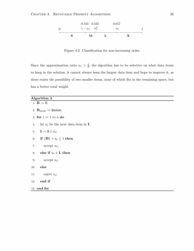
Chapter 4. Revocable Priority Algorithms 26
X
0
0.6570.432
1 − α1 α1
0.343
1α2
1
S M L
Figure 4.2: Classification for non-increasing order.
Since the approximation ratio α1 > 12, the algorithm has to be selective on what data items
to keep in the solution, it cannot always keep the largest data item and hope to improve it, as
there exists the possibility of two smaller items, none of which fits in the remaining space, but
has a better total weight.
Algorithm 2
1: B := ∅;
2: Bmode := Queue;
3: for i := 1 to n do
4: let ui be the next data item in I;
5: I := I⊖ ui;
6: if ‖B‖ + ui ≤ 1 then
7: accept ui;
8: else if ui ∈ L then
9: accept ui;
10: else
11: reject ui;
12: end if
13: end for

Chapter 4. Revocable Priority Algorithms 27
Proof of the Upper Bound
Theorem 4.2.2 There exists a non-increasing order revocable priority algorithm of SSP with
approximation ratio α1.
Proof: It is sufficient to show that Alg. 2 achieves this approximation ratio. We prove this by
induction on i. At the end of the ith iteration of the for loop, we let ALGi and OPTi be the
algorithm’s solution and the optimal solution respectively; these are solutions with respect to
the first i data items {u1, . . . , ui}. We also let ρi to be the current approximation ratio,
ρi =‖ALGi‖
‖OPTi‖.
It is clear that at the end of the first iteration, the algorithm has approximation ratio ρ1 = 1 >
α1. Suppose there is no early termination and the α1-approximation is maintained for the first
k − 1 iterations, i.e., ‖ALGi‖ < α1 and ρi ≥ α1 for all i < k; we examine the case for i = k,
k ≥ 2. Note that |ALGi| = 1 for all i < k, for otherwise ‖ALGi‖ ≥ α1. The algorithm examines
data items in non-increasing order; for data items in L, it always accepts the current one into
the solution, no matter whether or not the data item fits; for data items in M, it always rejects
the current one if it does not fit. In that sense, it tends to keep the smallest data item in L∩ I
and the largest data item in M ∩ I. There are only three possibilities for uk during the kth
iteration; it must fall into one of the lines 6, 8 and 10:
1. Line 6: then the algorithm accepts uk into the solution without discarding any accepted
data item in the solution. Hence we have |ALGi| = 2, the terminal condition is satisfied.
Therefore, the algorithm terminates and achieves approximation ratio α1.
2. Line 8: then at the end of (k − 1)th iteration, ALGk−1 contains only uk−1. Since the
terminal condition is not satisfied during the kth iteration, we have uk−1 + uk > 1.
Therefore, the algorithm accepts uk into the solution by discarding uk−1. Note that uk
and uk−1 are the two smallest data items examined so far and uk−1 +uk > 1, hence OPTk

Chapter 4. Revocable Priority Algorithms 28
contains exactly one data item, say ur, in L. Therefore, the approximation ratio is
ρk =‖ALGk‖
‖OPTk‖=
uk
ur
≥α2
1
α1
= α1.
3. Line 10: then uk ∈ M and the algorithm rejects uk, therefore ALGk = ALGk−1. Further-
more, at the end of (k − 1)th iteration, ALGk−1 contains exactly one data item. Observe
that it cannot be a data item in M; for otherwise, the terminal condition is satisfied.
Therefore, ALGk−1 contains exactly one data item, say uj, in L. Since the terminal con-
dition is not satisfied during the kth iteration, we have uk + uj > 1; then by equation
(3.1),
‖ALGk‖ = ‖ALGk−1‖ = uj > 1 − uk ≥ 1 − α21 = 2α3
1.
Note that for all the data items examined so far, uk is the smallest in M, uj is the smallest
in L, and uk + uj > 1, hence OPTk can either contain one data item in L or two data
items in M; in both cases ‖OPTk‖ < 2α21. Therefore, the approximation ratio is
ρk =‖ALGk‖
‖OPTk‖>
2α31
2α21
= α1.
We now have shown that in all three cases, the algorithm maintains the approximation ratio
ρi ≥ α1 for i = k; this completes the induction. Therefore, Alg. 2 achieves approximation ratio
α1.
Theorem 4.2.2 shows that, with the aid of revocable acceptance, we can improve the non-
increasing approximation ratio from 12
to α1 ≈ 0.657.
4.2.2 Non-Decreasing Order
One often tends to believe that non-increasing order is advantageous as it allows early exposure
of large data items, but it is not the case for fixed revocable priority algorithms. This is because
large data items, while not large enough to achieve the approximation ratio, need to take more

Chapter 4. Revocable Priority Algorithms 29
space; in other words, a fixed capacity takes less data items with large weight. Therefore, at
the time of an overflow, there are less data items in the solution, and hence less choices as to
which data items are rejected. Let α2 =√
17−1
4≈ 0.780 be the real root of the equation
2x2 + x − 2 = 0 (4.1)
between 0 and 1. In this subsection, we prove a tight bound of α2 on the approximation ratio
for non-decreasing order.
Theorem 4.2.3 No non-decreasing order revocable priority algorithm of SSP can achieve ap-
proximation ratio better than α2.
Proof: We show that for any non-decreasing order revocable priority algorithm and every small
ǫ > 0, ρ < α2 + ǫ. Let
u1 = 1 − α2 ≈ 0.220, u2 = 12α2 + 1
4ǫ ≈ 0.390, u3 = α2 ≈ 0.780;
we utilize the following adversarial strategy shown in Fig. 4.3.
⊕u2
⊕u1
u1
u1 2u2 u3
u32u2 u2u1 u2u2 u3
⊕u2,⊖u2
⊖u3
u1 u2s1 :
⊕u2,⊖u1
u32u2s2 :
⊘
⊘
⊘
Figure 4.3: Adversarial strategy for fixed non-decreasing order.
If the algorithm terminates via state s1, then ‖ALG‖ = u1 + u2 and ‖OPT‖ = 2u2. Note that,
by equation (4.1), we have u1 + u2 = 1 − 12α2 + 1
4ǫ = α2
2 + 14ǫ. Therefore, the approximation

Chapter 4. Revocable Priority Algorithms 30
ratio is
ρ =‖ALG‖
‖OPT‖=
u1 + u2
2u2
=1 − 1
2α2 + 1
4ǫ
α2 + 12ǫ
=α2
2 + 14ǫ
α2 + 12ǫ
< α2.
If the algorithm terminates via state s2, then ‖ALG‖ ≤ 2u2. Since u1 + u3 = 2 = 1, we have
‖OPT‖ = u1 + u3. Therefore, the approximation ratio is
ρ =‖ALG‖
‖OPT‖≤
2u2
u1 + u3
= α2 +1
2ǫ.
In both cases, the adversary forces the algorithm to have approximation ratio ρ < α2 + ǫ; this
completes the proof.
Description of the Algorithm
Next, we give a non-decreasing order revocable priority algorithm that achieves the approxi-
mation ratio α2. It is interesting that non-decreasing order can, to a large extent, improve the
approximation ratio. As we show later in this thesis, no fixed priority revocable algorithm can
achieve approximation ratio better than β1 ≈ 0.852; considering the fact that α2 ≈ 0.780 and
all previous priority algorithms studied have approximation ratios under the 23
mark, this is a
significant improvement.
We now describe the algorithm. For all possible relevant data items, we partition them into
two sets: M and L. A data item u is said to be in class M and L if 1 − α2 < u ≤ 12α2 and
12α2 < u < α2 respectively; see Fig. 4.4.
X
0 1α21 − α2
0.220 0.3901
2α2
0.780
S M L
Figure 4.4: Classification for non-decreasing order.
The algorithm achieves this ratio is surprisingly simple; it basically set Bmode to Stack mode,
and accepts each data item in turn; see Alg. 3.

Chapter 4. Revocable Priority Algorithms 31
Algorithm 3
1: B := ∅;
2: Bmode := Stack;
3: for i := 1 to n do
4: let ui be the next data item in I;
5: I := I⊖ ui;
6: accept ui;
7: end for
Proof of the Upper Bound
Theorem 4.2.4 There exists a non-decreasing order revocable priority algorithm of SSP with
approximation ratio α2.
Proof: It is sufficient to show that Alg. 3 achieves this approximation ratio. We prove this by
induction on i. At the end of the ith iteration of the for loop, we let ALGi and OPTi be the
algorithm’s solution and the optimal solution respectively; and let ρi be the current approxi-
mation ratio. It is clear that at the end of the first iteration, the algorithm has approximation
ratio ρ1 = 1 > α2. Suppose there is no early termination and the approximation ratio ρi ≥ α2
is maintained for all i < k, we examine the case for i = k. There are two possibilities. The first
case is that ‖B‖ + uk ≤ 1, then the algorithm accepts uk into the solution without discarding
any accepted data item in the solution. Hence we have ‖OPTk‖ ≥ ‖OPTk−1‖+uk; for otherwise,
we can take OPTk−1⊕uk as OPTk, which leads to a contradiction. Therefore, the approximation
ratio is
ρk =‖ALGk‖
‖OPTk‖≥
‖ALGk−1‖ + uk
‖OPTk−1‖ + uk
≥‖ALGk−1‖
‖OPTk−1‖= ρk−1 ≥ α2.
This leaves the case when ‖B‖ + uk > 1. Note that the algorithm examines data items in
non-decreasing order; u1 is the smallest data item in I and u2 is the second smallest. These

Chapter 4. Revocable Priority Algorithms 32
two data items are at the bottom of the stack, hence tend to stay in the stack unless we see a
data item with sufficient large weight:
• Observation 1: if at certain stage of the algorithm, after accepting uk, there is only one
data item uk 6= u1 in the stack, then we have u1 + uk > 1; see Fig. 4.5.
=u1
uk−1
ukuk⊕
Figure 4.5: Stack with one data item.
• Observation 2: if at certain stage of the algorithm, after accepting uk, there are only two
data items in the stack and the top of the stack is uk 6= u2, then we have u1 +u2 +uk > 1;
see Fig. 4.6.
=u2
u1
uk
uk
u1
uk−1
⊕
Figure 4.6: Stack with two data items.
The above two inequalities happen to be useful in our analysis. Now we consider data items in
OPTk; there are six cases:
1. If |OPTk| = 1, then OPTk = {uk}. Since the algorithm always accepts the current data
item, we have uk ∈ ALGk, and hence ALGk = OPTk. Therefore, the approximation ratio

Chapter 4. Revocable Priority Algorithms 33
is
ρk =‖ALGk‖
‖OPTk‖= 1.
2. If OPTk contains exactly two data items ur, us ∈ M with ur ≤ us, then we have both u1
and u2 in M ; we now consider data items in ALGk.
(a) If |ALGk| = 1, then ALGk = {uk}; by Observation 1, we have
u1 + uk > 1.
Note that ur + us ≤ α2 and by equation (4.1), we have 1 − u1 ≥ 1 − 12α2 = α2
2.
Therefore, the approximation ratio is
ρk =‖ALGk‖
‖OPTk‖=
uk
ur + us
>1 − u1
ur + us
≥α2
2
α2
= α2.
(b) If |ALGk| = 2, then ALGk = {u1, uk}; by Observation 2, we have
u1 + u2 + uk > 1.
Note that ur + us ≤ α2 and by equation (4.1), we have 1 − u2 ≥ 1 − 12α2 = α2
2.
Therefore, the approximation ratio is
ρk =‖ALGk‖
‖OPTk‖=
u1 + uk
ur + us
>1 − u2
ur + us
≥α2
2
α2
= α2.
(c) If |ALGk| ≥ 3, then {u1, u2, uk} ∈ ALG. Note that u1 + u2 > 2− 2α2. Therefore, the
approximation ratio is
ρk =‖ALGk‖
‖OPTk‖≥
u1 + u2 + uk
ur + us
>2 − 2α2 + us
12α2 + us
> 1,
which is a contradiction; this case is impossible.
3. If OPTk contains exactly two data items ur ∈ M and us ∈ L, then we have u1 in M ; we
now consider data items in ALGk.
Chapter 4. Revocable Priority Algorithms 34
(a) If |ALGk| = 1, then ALGk = {uk}; by Observation 1, we have
u1 + uk > 1. (4.2)
Note that u1 + us ≤ ur + us ≤ 1. When the algorithm considers us, u1 is already in
the solution. Since the terminal condition is not satisfied, we have
u1 + us < α2. (4.3)
Combining (4.2) and (4.3), we have uk > 1 − α2 + us. Therefore,
ρk =‖ALGk‖
‖OPTk‖=
uk
ur + us
>1 − α2 + us
12α2 + us
>1 − α2 + 1
2α2
12α2 + 1
2α2
=1 − 1
2α2
α2
.
By equation (4.1), the approximation ratio is
ρk >1 − 1
2α2
α2
=α2
2
α2
= α2.
(b) If |ALGk| = 2, then ALGk = {u1, uk}. Therefore
ρk =‖ALGk‖
‖OPTk‖=
u1 + uk
ur + us
>1 − α2 + us
12α2 + us
>1 − α2 + 1
2α2
12α2 + 1
2α2
=1 − 1
2α2
α2
.
By equation (4.1), the approximation ratio is
ρk >1 − 1
2α2
α2
=α2
2
α2
= α2.
(c) If |ALGk| ≥ 3, then {u1, u2, uk} ∈ ALG. Note that u1 + u2 > 2− 2α2. Therefore, the
approximation ratio is
ρk =‖ALGk‖
‖OPTk‖≥
u1 + u2 + uk
ur + us
>2 − 2α2 + us
12α2 + us
> 1,
which is a contradiction; this case is impossible.
4. If OPTk contains exactly two data items ur, us ∈ L with ur ≤ us, then we have
α2 ≤ ur + ur+1 ≤ ur + us ≤ 1.
When the algorithm considers ur+1, ur is already in the solution; hence the terminal
condition is satisfied.
Chapter 4. Revocable Priority Algorithms 35
5. If OPTk contains exactly three data items ur, us, ut ∈ M with ur ≤ us ≤ ut, then we have
both u1 and u2 in M ; we now consider data items in ALGk.
(a) If |ALGk| = 1, then ALGk = {uk}; by Observation 1, we have
u1 + uk > 1. (4.4)
Note that u1 + ur + us ≤ u1 + us + us+1 ≤ ur + us + ut ≤ 1. When the algorithm
considers us+1, u1 and us are already in the solution. Since the terminal condition
is not satisfied, we have u1 + us + us+1 < α2. Therefore,
u1 + ur + us < α2. (4.5)
Combining (4.4) and (4.5), we have uk > 1−α2 + ur + us. Since both ur and us are
in M, we have ur + us > 2 − 2α2 > 12α2. Therefore,
ρk =‖ALGk‖
‖OPTk‖=
uk
ur + us + ut
>1 − α2 + (ur + us)
12α2 + (ur + us)
>1 − α2 + 1
2α2
12α2 + 1
2α2
=1 − 1
2α2
α2
.
By equation (4.1), the approximation ratio is
ρk >1 − 1
2α2
α2
=α2
2
α2
= α2.
(b) If |ALGk| = 2, then ALGk = {u1, uk}; by Observation 2, we have
u1 + u2 + uk > 1. (4.6)
• If r = 1, then u2 + ur + us ≤ u1 + u2 + us+1 ≤ ur + us + ut ≤ 1. When
the algorithm considers us+1, u1 and u2 are already in the solution. Since the
terminal condition is not satisfied, we have u1 + u2 + us+1 < α2. Therefore,
u2 + ur + us < α2. (4.7)
• If r > 1, then u2 + ur + us ≤ u2 + us + us+1 ≤ ur + us + ut ≤ 1. When
the algorithm considers us+1, u2 and us are already in the solution. Since the
terminal condition is not satisfied, we have u2 + us + us+1 < α2. Therefore, the
inequality (4.7) is also satisfied.

Chapter 4. Revocable Priority Algorithms 36
Therefore, in both cases we have (4.7). Combining (4.6) and (4.7), we have u1+uk >
1− α2 + ur + us. Since both ur and us are in M, we have ur + us > 2− 2α2 > 12α2.
Therefore,
ρk =‖ALGk‖
‖OPTk‖=
u1 + uk
ur + us + ut
>1 − α2 + (ur + us)
12α2 + (ur + us)
>1 − α2 + 1
2α2
12α2 + 1
2α2
=1 − 1
2α2
α2
.
By equation (4.1), the approximation ratio is
ρk >1 − 1
2α2
α2
=α2
2
α2
= α2.
(c) If |ALGk| ≥ 3, then {u1, u2, uk} ⊆ ALG. Note that u1 + ur + us ≤ u1 + us + us+1 ≤
ur + us + ut ≤ 1. When the algorithm considers us+1, u1 and us are already in the
solution. Since the terminal condition is not satisfied, we have u1 + us + us+1 < α2.
Therefore,
u1 + ur + us < α2. (4.8)
By (4.8), we have ur + us < α2 − u1 < α2 − (1 − α2) = 2α2 − 1. Note that
u1 + u2 > 2 − 2α2. Therefore,
ρk =‖ALGk‖
‖OPTk‖≥
u1 + u2 + uk
ur + us + ut
>2 − 2α2 + ut
2α2 − 1 + ut
>2 − 2α2 + 1 − α2
2α2 − 1 + 1 − α2
=3 − 3α2
α2
.
Since 3 − 3α2 > α22, the approximation ratio is
ρk >3 − 3α2
α2
> α2.
6. If OPTk contains exactly three data items ur, us ∈ M and ut ∈ L with ur ≤ us, then we
have
α2 < 2 − 2α2 +1
2α2 < u1 + u2 + ut ≤ ur + us + ut ≤ 1.
When the algorithm considers ut, u1 and u2 are already in the solution; hence the terminal
condition is satisfied.

Chapter 4. Revocable Priority Algorithms 37
We now have shown that in all six cases, the algorithm maintains the approximation ratio
ρi ≥ α2 for i = k; this completes the induction. Therefore, Alg. 3 achieves approximation ratio
α2.
Theorem 4.2.4 shows the existence of a simple non-decreasing order revocable priority al-
gorithm which achieves the approximation ratio α2 ≈ 0.780. This bound is better than any
“greedy” algorithm discussed so far in this thesis, and it surpasses the multi-pass greedy algo-
rithm by Martello and Toth mentioned in Section 1.1.
4.2.3 A General Lower Bound
Let β1 =√
145+5
20≈ 0.852 be the real root of the equation
10x2 − 5x − 3 = 0 (4.9)
between 0 and 1. In this subsection, we prove a lower bound of β1 on the approximation ratio
for general fixed revocable priority algorithms.
Theorem 4.2.5 No fixed revocable priority algorithm of SSP can achieve approximation ratio
better than β1.
Proof: Let
u1 = 15
= 0.200, u2 = 12β1 −
110
≈ 0.326,
u3 = 12
= 0.500, u4 = 45
= 0.800;
For a data item u, we denote by rank(u) its priority assigned by algorithm A. There are four
cases:
1. If rank(u2) > rank(u1), then we utilize the following adversarial strategy shown in
Fig. 4.7; we omit the starting few states where overflow does not occur.

Chapter 4. Revocable Priority Algorithms 38
u1
⊘⊕u1,⊖u1
⊘⊕u1,⊖u1
⊘⊕u1,⊖u1
⊕u1,⊖u2
⊖3u1
u12u2 u12u2 2u1
2u2 u1
⊕u1,⊖u2
s1 : s2 :u2 2u1
2u2 u1 4u1 3u1
⊖2u1
⊕u1,⊖u2
⊖u1
Figure 4.7: Adversarial strategy for rank(u2) > rank(u1).
If the algorithm terminates via state s1, then ‖ALG‖ = 2u1 + u2 and ‖OPT‖ ≥ u1 + 2u2.
Therefore,
ρ =‖ALG‖
‖OPT‖≤
2u1 + u2
u1 + 2u2
=25
+ 12β1 −
110
15
+ β1 −15
=12β1 + 3
10
β1
=5β1 + 3
10β1
.
By equation (4.9), the approximation ratio is
ρ ≤5β1 + 3
10β1
= β1.
If the algorithm terminates via state s2, then ‖ALG‖ ≤ u1 + 2u2 and ‖OPT‖ = 5u1.
Therefore, the approximation ratio is
ρ =‖ALG‖
‖OPT‖≤
u1 + 2u2
5u1
= u1 + 2u2 =1
5+ β1 −
1
5= β1.
Therefore, if A ranks u2 before u1, then the adversary can force it to have approximation
ratio no better than β1.
2. If rank(u3) > rank(u2), then we utilize the following adversarial strategy shown in
Fig. 4.8; we omit the starting few states where overflow does not occur.
If the algorithm terminates via state s1, then ‖ALG‖ = 2u2 and ‖OPT‖ = u2 + u3.
Therefore, the approximation ratio is
ρ =‖ALG‖
‖OPT‖=
2u2
u2 + u3
=β1 −
15
12
+ 12β1 −
110
=10β1 − 2
5β1 + 4< β1.

Chapter 4. Revocable Priority Algorithms 39
u2
⊘⊕u2,⊖u2
u2 2u2u3
u3 u2s1 : s2 :2u2
⊕u2,⊖u3
⊖u2
Figure 4.8: Adversarial strategy for rank(u3) > rank(u2).
If the algorithm terminates via state s2, then ‖ALG‖ ≤ u2 + u3 and ‖OPT‖ = 3u2.
Therefore, the approximation ratio is
ρ =‖ALG‖
‖OPT‖≤
u2 + u3
3u2
=12
+ 12β1 −
110
32β1 −
310
=5β1 + 4
15β1 − 3< β1.
Therefore, if A ranks u3 before u2, then the adversary can force it to have approximation
ratio no better than β1.
3. If rank(u4) > rank(u3), then we utilize the following adversarial strategy shown in
Fig. 4.9; we omit the starting few states where overflow does not occur.
u3s1 : u3
u4 2u3
⊕u3,⊖u4
⊖u3
u4s2 :
⊘⊕u3,⊖u3
Figure 4.9: Adversarial strategy for rank(u4) > rank(u3).
If the algorithm terminates via state s1, then ‖ALG‖ = u3 and ‖OPT‖ = u4. Therefore,
the approximation ratio is
ρ =‖ALG‖
‖OPT‖=
u3
u4
< β1.
If the algorithm terminates via state s2, then ‖ALG‖ ≤ u4 and ‖OPT‖ = 2u3. Therefore,

Chapter 4. Revocable Priority Algorithms 40
the approximation ratio is
ρ =‖ALG‖
‖OPT‖≤
u4
2u3
= u4 < β1.
Therefore, if A ranks u4 before u3, then the adversary can force it to have approximation
ratio no better than β1.
4. If rank(u1) > rank(u2) > rank(u3) > rank(u4), then we utilize the following adversarial
strategy shown in Fig. 4.10; we omit the starting few states where overflow does not occur.
⊕u3,⊖u2
u2
s1 : u1
u1 u3
u3
u4
⊕u3,⊖u1
⊘
u4u3 u2s2 :
⊖u4
Figure 4.10: Adversarial strategy for rank(u1) > rank(u2) > rank(u3) > rank(u4).
If the algorithm terminates via state s1, then ‖ALG‖ = u1 + u3 and ‖OPT‖ = u2 + u3.
Therefore, the approximation ratio is
ρ =‖ALG‖
‖OPT‖=
u1 + u3
u2 + u3
=15
+ 12
1
2β1 −
1
10+ 1
2
=7
5β1 + 4< β1.
If the algorithm terminates via state s2, then ‖ALG‖ ≤ u2 + u3 and ‖OPT‖ = u1 + u4.
Therefore, the approximation ratio is
ρ =‖ALG‖
‖OPT‖≤
u2 + u3
u1 + u4
= u2 + u3 =1
2β1 −
1
10+
1
2< β1.
Therefore if A ranks rank(u1) > rank(u2) > rank(u3) > rank(u4), then the adversary
can force it to have approximation ratio no better than β1.

Chapter 4. Revocable Priority Algorithms 41
As a conclusion, no fixed revocable priority algorithm of SSP can achieve approximation ratio
better than β1. This completes the proof.
This lower bound β1 ≈ 0.852 for fixed revocable priority algorithms of SSP is interesting as
it shows the first gap we are unable to close. The analysis above is relatively tight in cases 1,
2 and 4, and there seems not much room left for improvement. Intuitively, though, it is quite
promising that this gap can be closed, but this may require more sophisticated adversaries,
which might involve a large set of data items, and more carefully designed algorithms.
4.3 Adaptive Revocable Priority Algorithms
Adaptive priority algorithms are more powerful than fixed priority algorithms in the sense
that remaining data items can be reordered at each iteration. In this section, we provide an
adaptive revocable priority algorithm of SSP which has a better approximation ratio than the
fixed revocable priority algorithms discussed in the previous section. We also prove a lower
bound on the approximation ratio for the adaptive case.
4.3.1 Deriving a Lower Bound
Let β2 =√
19+1
6≈ 0.893 be the real root of the equation
6x2 − 2x − 3 = 0 (4.10)
between 0 and 1. In this subsection, we prove a lower bound of β2 on the approximation ratio
for adaptive revocable priority algorithms.
Theorem 4.3.1 No adaptive revocable priority algorithm of SSP can achieve approximation
ratio better than β2.
Proof: Suppose there exists an algorithm A such that ρ > β2. Let
u1 = 13β2 ≈ 0.298, u3 = 1
2= 0.500;
Chapter 4. Revocable Priority Algorithms 42
We utilize the following adversary strategy shown in Fig. 4.11.
⊘
2u2
u1
u1
u1
u1
u2
u2
u2
u2
⊕u1
⊕u2
⊕u2
2u1
3u1
3u1
2u1
2u1 2u2 3u1
u1
u1 u2
2u2 2u1
u1 2u1
u2
⊕u1
⊕u1
⊕u1,⊖u2⊕u1,⊖u1⊕u1⊕u2,⊖u2 ⊕u2,⊖u1
⊕u2,⊖2u1 ⊕u2,⊖u2
⊖u2
⊖u2
⊖u2 ⊖u1
⊖u2
s1 : s3 : s5 :
s2 :s4 :
2u2
⊘
⊘
⊘ ⊘ ⊘
⊘
3u1
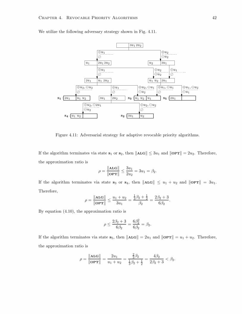
Figure 4.11: Adversarial strategy for adaptive revocable priority algorithms.
If the algorithm terminates via state s1 or s2, then ‖ALG‖ ≤ 3u1 and ‖OPT‖ = 2u2. Therefore,
the approximation ratio is
ρ =‖ALG‖
‖OPT‖≤
3u1
2u2
= 3u1 = β2.
If the algorithm terminates via state s3 or s4, then ‖ALG‖ ≤ u1 + u2 and ‖OPT‖ = 3u1.
Therefore,
ρ =‖ALG‖
‖OPT‖≤
u1 + u2
3u1
=1
3β2 + 1
2
β2
=2β2 + 3
6β2
.
By equation (4.10), the approximation ratio is
ρ ≤2β2 + 3
6β2
=6β2
2
6β2
= β2.
If the algorithm terminates via state s5, then ‖ALG‖ = 2u1 and ‖OPT‖ = u1 + u2. Therefore,
the approximation ratio is
ρ =‖ALG‖
‖OPT‖=
2u1
u1 + u2
=23β2
13β2 + 1
2
=4β2
2β2 + 3< β2.

Chapter 4. Revocable Priority Algorithms 43
In all three cases, the adversary forces the algorithm A to have approximation ratio no better
than β2; this completes the proof.
4.3.2 A Better Algorithm
In this subsection, we give an adaptive revocable priority algorithm that achieves the approxi-
mation ratio of α3 = 0.8. This is the most involved algorithm in this thesis. Similar to previous
cases, we partition all possible relevant data items into sets: M and L. A data item u is said
to be in class M and L if 0.2 < u ≤ 0.4 and 0.4 < u < 0.8 respectively; see Fig. 4.12.
S
0 10.80.4
M
0.2 0.3
M1 M2
L X
Figure 4.12: Classification for the adaptive revocable priority algorithm.
For notational convenience, we further divide the class M into two sets. A data item u is said
to be in class M1, M2 if 0.2 < u ≤ 0.3, 0.3 < u ≤ 0.4 respectively. We call our algorithm
ADAPTIVE, and use the following symbols to denote data items in different classes; see Table 4.1
Table 4.1: Corresponding symbols.
class M L M1 M2
symbol ♦ � ▽ △
The algorithm ADAPTIVE includes two stages; data items in M are processed during the first
stage and data items in L are processed during the second stage. The ordering of data items
(in each stage) is determined by its distance to the middle point of M, i.e., the closer a data
item to 0.3, the higher its priority is. The algorithm is described below.
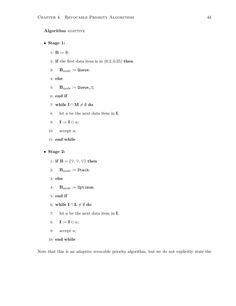
Chapter 4. Revocable Priority Algorithms 44
Algorithm ADAPTIVE
• Stage 1:
1: B := ∅;
2: if the first data item is in (0.2, 0.35) then
3: Bmode := Queue;
4: else
5: Bmode := Queue_1;
6: end if
7: while I ∩M 6= ∅ do
8: let u be the next data item in I;
9: I := I ⊖ u;
10: accept u;
11: end while
• Stage 2:
1: if B = {▽,▽,▽} then
2: Bmode := Stack;
3: else
4: Bmode := Optimum;
5: end if
6: while I ∩ L 6= ∅ do
7: let u be the next data item in I;
8: I := I ⊖ u;
9: accept u;
10: end while
Note that this is an adaptive revocable priority algorithm, but we do not explicitly state the

Chapter 4. Revocable Priority Algorithms 45
terminal condition in the algorithm. If at a certain step of the algorithm, the terminal condition
is satisfied, the data item which contributes to this satisfaction will be the next data item and
interrupt the ordering. Let S = u1, u2, . . . , un be the input sequence of data items according to
this ordering, and let S1 = u1, u2, . . . , um and S2 = um+1, um+2, . . . , un be the input sequences
of data items for the first stage and second stage respectively. From now on, we assume that the
algorithm ADAPTIVE achieves approximation ratio less than 0.8 and try to derive a contradiction.
Lemma 4.3.2 Let u be the next data item to be examined and B′ = (B ⊕ u). If B′ contains
three data items ui, uj, uk, with i < j < k, then (ui, uj , uk) cannot be any of the following
types:
(▽,▽,△), (▽,△,▽),
(△,△,▽), (△,▽,△);
Proof: We show that if (ui, uj , uk) is one of the above types, then 0.8 ≤ ui + uj + uk ≤ 1,
which is a contradiction.
1. If (ui, uj , uk) = (▽,▽,△), then since j < k, we have 0.6 ≤ uj +uk ≤ 0.7. Since 0.2 ≤ ui ≤
0.3, we have 0.8 ≤ ui + uj + uk ≤ 1.
2. If (ui, uj , uk) = (▽,△,▽), then since i < j, we have 0.6 ≤ ui + uj ≤ 0.7. Since 0.2 ≤ uk ≤
0.3, we have 0.8 ≤ ui + uj + uk ≤ 1.
3. If (ui, uj , uk) = (△,△,▽), then since j < k, we have 0.5 ≤ uj +uk ≤ 0.6. Since 0.3 ≤ ui ≤
0.4, we have 0.8 ≤ ui + uj + uk ≤ 1.
4. If (ui, uj , uk) = (△,▽,△), then since i < j, we have 0.5 ≤ ui + uj ≤ 0.6. Since 0.3 ≤ uk ≤
0.4, we have 0.8 ≤ ui + uj + uk ≤ 1.
Therefore, (ui, uj , uk) cannot be any of the above types.
Lemma 4.3.3 The input sequence S1 = u1, . . . , um is a subsequence of one of the following
sequence types:
Chapter 4. Revocable Priority Algorithms 46
1. ▽,▽,▽, . . . ,▽,▽,▽
2. △,▽,▽, . . . ,▽,▽,▽
3. △,△,△, . . . ,△,△,△
4. ▽,△,△, . . . ,△,△,△
Proof: If S1 contains at most two data items, then it is a subsequence of one of the four
sequence types above. Suppose now S1 contains more than two data items; there are four
cases:
1. If (u1, u2) = (▽,▽), then B is in Queue Mode for the first stage. Suppose △ occurs
after u2, then let ui+1 be the first such occurrence; when the algorithm considers ui+1,
{ui−1, ui} ⊆ B. Since (ui−1, ui, ui+1) = (▽,▽,△), this contradicts Lemma 4.3.2.
2. If (u1, u2) = (▽,△), then B is in Queue Mode for the first stage. Suppose ▽ occurs
after u2, then let ui+1 be the first such occurrence; when the algorithm considers ui+1,
{ui−1, ui} ⊆ B. Since either (ui−1, ui, ui+1) = (△,△,▽), or (ui−1, ui, ui+1) = (▽,△,▽),
this contradicts Lemma 4.3.2.
3. If (u1, u2) = (△,▽), then we have two cases:
(a) If u1 < 0.35, then B is in Queue Mode for the first stage. Suppose △ occurs after
u2, then let ui+1 be the first such occurrence; when the algorithm considers ui+1,
{ui−1, ui} ⊆ B. Since either (ui−1, ui, ui+1) = (▽,▽,△), or (ui−1, ui, ui+1) = (△
,▽,△), this contradicts Lemma 4.3.2.
(b) If u1 ≥ 0.35 then B is in Queue_1 Mode for the first stage. Suppose △ occurs after
u2, then let ui+1 be the first such occurrence; when the algorithm considers ui+1,
{u1, ui} ⊆ B. Since (u1, ui, ui+1) = (△,▽,△), this contradicts Lemma 4.3.2.
4. If (u1, u2) = (△,△), then we have two cases:

Chapter 4. Revocable Priority Algorithms 47
(a) If u1 < 0.35, then B is in Queue Mode for the first stage. Suppose ▽ occurs after
u2, then let ui+1 be the first such occurrence; when the algorithm considers ui+1,
{ui−1, ui} ⊆ B. Since (ui−1, ui, ui+1) = (△,△,▽), this contradicts Lemma 4.3.2.
(b) If u1 ≥ 0.35, then B is in Queue_1 Mode for the first stage. Suppose ▽ occurs after
u2, then let ui+1 be the first such occurrence; when the algorithm considers ui+1,
{u1, ui} ⊆ B. Since (u1, ui, ui+1) = (△,△,▽), this contradicts Lemma 4.3.2.
Therefore, S1 must be a subsequence of one of the input sequence types above.
Lemma 4.3.3 is useful as it eliminates many cases we need to consider. We now give two
observations:
• Observation 3: for the input sequence types 1 and 2, the data items in S1 is non-
increasing, and the total weight of the first three data items of S1 is no greater than
1.
• Observation 4: for the input sequence types 3 and 4, the data items in S1 is non-
decreasing. and the total weight of the first three data items of S1 is greater than 0.8.
The data items in S2 is non-decreasing in both cases. For convenience, we denote ALG′ the
algorithm’s solution at the end of the first stage; we also suppose S is non-empty, for otherwise
the problem becomes trivial.
Lemma 4.3.4 |OPT| > 1.
Proof: Suppose now |OPT| = 1, there are two cases:
1. If S contains a data item of type �, then un is the largest data item in S and OPT = {un}.
No matter which operational mode B is in, un is always accepted into the solution. Since
un is the last data item in S, the algorithm achieves the optimal solution in this case,
which is a contradiction.

Chapter 4. Revocable Priority Algorithms 48
2. If S does not contain a data item of type �, then the entire input sequence S contain
exactly one data item of type ♦, hence the algorithm easily achieves the optimal solution,
which is a contradiction.
Therefore, both cases are impossible, and hence |OPT| > 1.
Lemma 4.3.5 No feasible solution contains two data items in S2.
Proof: We prove this by contradiction. Suppose there is a feasible solution which contains two
data items in S2, then it is clear that 0.8 ≤ um+1 + um+2 ≤ 1, and um+1 ≤ 0.5; we exam the
beginning of the second stage when the algorithm considers um+1. Note that the algorithm
has to reject um+1, for otherwise, when the algorithm considers the next data item um+2, the
terminal condition is satisfied.
1. If |ALG′| < 2, then ‖ALG
′‖ ≤ 0.4. Since ‖ALG′‖ + um+1 ≤ 1, the algorithm must then
accept um+1 into its solution, which is a contradiction.
2. If |ALG′| = 2, then B is in Optimum Mode for the second stage. Let ALG
′ = {ui, uj}, then
we have ui + uj < uj + um+1 < um+1 + um+2 ≤ 1, the algorithm must then accept um+1
into its solution, which is a contradiction.
3. If |ALG′| = 3, then we have S1 is a subsequence of either input sequence type 1 or 2;
for otherwise, by Lemma 4.3.3, either ALG′ = {△,△,△} or ALG
′ = {▽,△,△}, and hence
‖ALG′‖ > 0.8, which is a contradiction.
(a) If ALG′ = {△,▽,▽}, then ALG
′ = {u1, um−1, um}. Since u1 ≥ 0.3, we have
0.4 ≤ um−1 + um ≤ 0.5. (4.11)
If there exist a data item in [0.4, 0.5], then combined with (4.11), that data item will
interrupt the ordering and the terminal condition is satisfied. Hence, there exists no
data item in [0.4, 0.5], Therefore, No feasible solution contains two data items in S2.
Chapter 4. Revocable Priority Algorithms 49
(b) If ALG′ = {▽,▽,▽}, then during the second stage, B is in Stack Mode, hence the
algorithm must then accept um+1 into its solution, which is a contradiction.
Therefore, no feasible solution contains two data items in S2. This completes the proof.
Lemma 4.3.6 |OPT| < 4 ⇒ ‖OPT‖ < 0.8.
Proof: We prove this by contradiction. Suppose that |OPT| < 4 and ‖OPT‖ ≥ 0.8; by
Lemma 4.3.4, |OPT| > 1. There are two cases:
1. If |OPT| = 2, then let OPT = {ur, us} with ur ≤ us. Note that if (ur, us) = (�,�), then it
contradicts Lemma 4.3.5. Therefore (ur, us) = (♦,�), then ur always enters the solution.
This is because during the first stage, B is either in Queue_1 Mode or Queue Mode, every
data item in S1 gets a chance to enter the solution. Since ur + us ≥ 0.8, us will interrupt
the ordering and become the next data item to be examined when ur is in B, hence the
terminal condition is satisfied; this is a contradiction.
2. If |OPT| = 3, then let OPT = {ur, us, ut} with ur ≤ us ≤ ut, there are two possibilities:
(a) If (ur, us, ut) = (♦,♦,♦), then consider the first three elements in S. If S1 is a
subsequence of either input sequence type 1 or 2, then by Observation 3, we have
0.8 ≤ ur + us + ut ≤ u1 + u2 + u3 ≤ 1.
Therefore, the terminal condition is satisfied when the algorithm accepts the first,
second and third data item; this is a contradiction. If S1 is a subsequence of either
input sequence type 3 or 4, then by Observation 4, we have
0.8 ≤ u1 + u2 + u3 ≤ ur + us + ut ≤ 1.
Therefore, the terminal condition is satisfied when the algorithm accepts the first,
second and third data item; this is a contradiction.

Chapter 4. Revocable Priority Algorithms 50
(b) If (ur, us, ut) = (♦,♦,�), then consider the input sequence S. If S1 is a subsequence
of either input sequence type 1 or 2, then at the end of the first stage, {um−1, um} ⊆
ALG′. Since um−1 and um are the two smallest data items, we have
0.8 ≤ um−1 + um + ut ≤ ur + us + ut ≤ 1.
Therefore, the terminal condition is satisfied at the end of the first stage; this is a
contradiction. If S1 is a subsequence of either input sequence type 3 or 4, then by
Observation 4, we have
0.8 ≤ u1 + u2 + u3 ≤ ur + us + ut ≤ 1.
Therefore, the terminal condition is satisfied when the algorithm accepts the first,
second and third data item; this is a contradiction.
Therefore, ‖OPT‖ < 0.8. This completes the proof.
Lemma 4.3.7 Bmode = Optimum ⇒ ‖ALG′‖ < 0.8‖OPT‖.
Proof: Suppose that ‖ALG′‖ ≥ 0.8‖OPT‖, then since B in Optimum Mode during the second
stage, ‖B‖ is non-decreasing. Therefore ‖ALG′‖ ≤ ‖ALG‖, the approximation ratio is
ρ =‖ALG‖
‖OPT‖≥
‖ALG′‖
‖OPT‖≥ 0.8,
which is a contradiction.
Lemma 4.3.8 |ALG′| 6= 0.
Proof: Suppose that |ALG′| = 0, then S1 is empty. By Lemma 4.3.4, |OPT| > 1, hence OPT
contains at least two data items in S2; this contradicts Lemma 4.3.5. Therefore, |ALG′| 6= 0.
Lemma 4.3.9 |ALG′| 6= 1.
Chapter 4. Revocable Priority Algorithms 51
Proof: Suppose that |ALG′| = 1, then S1 contains only one data item. By Lemmas 4.3.4
and 4.3.5, |OPT| > 1, and OPT contains at most one data item in S2. Therefore OPT = {u1, ui}.
Since B is in Optimum Mode, then by Lemma 4.3.5, the algorithm achieves the optimal solution,
which is a contradiction. Therefore, |ALG′| 6= 1.
Lemma 4.3.10 |ALG′| 6= 2.
Proof: Suppose that |ALG′| = 2, then |OPT| < 4. This is because if |OPT| = 4, S1 is a
subsequence of either input sequence type 1 or 2, and hence |ALG′| = 3, which is a contradiction.
By Lemma 4.3.4, |OPT| > 1. There are two cases:
1. If |OPT| = 2, then let OPT = {ur, us} with ur ≤ us. By Lemma 4.3.5 and 4.3.6, ur is in
S1 and ‖OPT‖ < 0.8; there are two possibilities:
(a) If (ur, us) = (♦,♦), then if m = 2, then ur and us are the only two data items
in S1 and ALG′ = {ur, us}. Since B is in Optimum Mode during the second stage,
the algorithm clearly achieves the optimal solution, which is a contradiction. If
m > 2, then S1 is a subsequence of either input sequence type 3 or 4; for otherwise,
|ALG′| > 2. Therefore ALG
′ = {ui, um}, where ui > 0.3; hence we have
‖ALG′‖
‖OPT‖=
ui + um
ur + us
>0.3 + um
2um
≥0.7
0.8> 0.8.
Since B is in Optimum Mode during the second stage, by Lemma 4.3.7, we have
‖ALG′‖ < 0.8‖OPT‖, which is contradiction.
(b) If (ur, us) = (♦,�), then ur must be the largest data item in S1. This is because
‖OPT‖ = ur + us < 0.8. If ur is not the largest data item in S1, we can always
replace it with the largest data item in S1; the solution can only increase, and the
feasibility is still maintained. If m = 2, then ur ∈ ALG′. If m > 2, then S belongs
to either input sequence 3 or 4; for otherwise, |ALG′| > 2. Therefore, we also have

Chapter 4. Revocable Priority Algorithms 52
ur ∈ ALG′. Since B is in Optimum Mode during the second stage, by Lemma 4.3.5,
the algorithm achieves the optimal solution, which is also a contradiction.
2. If |OPT| = 3, then let OPT = {ur, us, ut} with ur ≤ us ≤ ut, there are two possibilities:
(a) If ALG′ = {▽,▽} or ALG
′ = {▽,△}, then S1 is a subsequence of input sequence type
1, 2 or 4, and S1 contains only two data items. We then have
0.8 ≤ u1 + u2 + u3 ≤ ur + us + ut ≤ 1.
Therefore, the terminal condition is satisfied, which is a contradiction.
(b) If ALG′ = {△,△}, then S1 is a subsequence of either input sequence type 3 or 4,
hence |OPT| < 3, which is a contradiction.
Therefore, |ALG′| 6= 2.
Lemma 4.3.11 |ALG′| 6= 3.
Proof: Suppose that |ALG′| = 3, then S1 is a subsequence of either input sequence type 1 or
2; for otherwise, by Lemma 4.3.3, either ALG′ = {△,△,△} or ALG
′ = {▽,△,△}, and hence
‖ALG′‖ > 0.8, the terminal condition is satisfied, which is a contradiction.
1. If ALG′ = {△,▽,▽}, then ALG
′ = {u1, um−1, um}; there are two cases:
(a) If |OPT| < 4, then by Lemma 4.3.6, we have
‖OPT‖ < 0.8.
Since we have B in Optimum Mode during the second stage and
‖ALG′‖ = u1 + um−1 + um > 0.7,
this contradicts Lemma 4.3.7.

Chapter 4. Revocable Priority Algorithms 53
(b) If |OPT| = 4, then if B in Queue Mode during the first stage, then |ALG′| = 4, which
is a contradiction. Therefore, B in Queue_1 Mode during the first stage. If u1 ∈ OPT,
then |ALG′| = 4, which is a contradiction. Therefore, u1 6∈ OPT; by Observation 3,
‖OPT‖ ≤ u2 + u3 + u4 + u5. Note that at the same time, we have the following three
inequalities:
u1 ≥ 0.35, (4.12)
u1 + u2 + u3 < 0.8, (4.13)
u2 + u3 ≥ u4 + u5. (4.14)
Combining (4.12) and (4.13), we have u2 + u3 < 0.45. Therefore, by (4.14),
‖OPT‖ ≤ u2 + u3 + u4 + u5 ≤ 2(u2 + u3) < 0.9.
Since we have B in Optimum Mode during the second stage and
‖ALG′‖ = u1 + um−1 + um > 0.75,
this contradicts Lemma 4.3.7.
2. If ALG′ = {▽,▽,▽}, then ALG
′ = {um−2, um−1, um}; there are two cases:
(a) If S2 is empty, then there two possibilities. If m = 3, then the algorithm clearly
achieves the optimal solution. If m > 3, then ‖ALG‖ > 0.65. Since um−2, um−1 and
um are the three smallest data items in S, we have |OPT| < 4. By Lemma 4.3.6,
‖OPT‖ < 0.8. Therefore, the approximation ratio is
ρ =‖ALG‖
‖OPT‖>
0.65
0.8≥ 0.8,
which is a contradiction.
(b) If S2 is non-empty, then since um−2, um−1 and um are the three smallest data items
in S, we have |OPT| < 4. By Lemma 4.3.6, ‖OPT‖ < 0.8. Since B in Stack Mode
Chapter 4. Revocable Priority Algorithms 54
during the second stage and um ≤ um−1 ≤ um−2 ≤ 0.3, we then have ‖ALG‖ > 0.7.
Therefore, the approximation ratio is
ρ =‖ALG‖
‖OPT‖>
0.7
0.8≥ 0.8,
which is a contradiction.
Therefore, |ALG′| 6= 3.
Now we are ready to prove the main theorem. Recall that all Lemmas 4.3.8, 4.3.9, 4.3.10,
and 4.3.11 are assuming the algorithm ADAPTIVE achieves approximation ratio less than 0.8.
Theorem 4.3.12 There exists an adaptive revocable priority algorithm of SSP with approxi-
mation ratio 0.8.
Proof: It is sufficient to show that the algorithm ADAPTIVE achieves this approximation ratio.
We prove this by contradiction. Suppose the algorithm ADAPTIVE achieves approximation ratio
less than 0.8, then by Lemmas 4.3.8, 4.3.9, 4.3.10, and 4.3.11, we have |ALG′| ≥ 4. This satisfies
the terminal condition, hence a contradiction. Therefore, the algorithm ADAPTIVE achieves
approximation ratio 0.8.
Chapter 5
Conclusion
5.1 Summary of Results
This work studies priority algorithms for the Subset-Sum Problem with the main focus on their
approximation ratios. Different classes of priority algorithms are analyzed and corresponding
lower bounds are proved. Although we are unable to close the two gaps we have for fixed
and adaptive revocable priority algorithms, this work gives us some basic understandings of
the relative power the Priority Model, and how revocable acceptances increase the algorithm’s
approximation ability.
The thesis starts with irrevocable priority algorithms, shows tight approximation ratio for
this class, regardless of whether it is fixed or adaptive. It then moves onto revocable priority
algorithms, in the spirit of algorithms with revocable acceptances studied in [17, 19]. Fixed
revocable priority algorithms with non-increasing and non-decreasing order are subsequently
studied; both with tight bounds on the approximation ratios. Then a general lower bound
for fixed revocable priority algorithms is given, exhibiting the first gap that we are unable to
close in this thesis. Finally, the class of adaptive revocable priority algorithms, a more complex
structure, is studied. A pair of unmatched upper and lower bound is provided, illustrating the
second unclosed gap. A list of results is summarized in Table 5.1, where the corresponding
55

Chapter 5. Conclusion 56
values are given in Table 5.2.
Table 5.1: Summary of results.
irrevocable revocable
fixed ρ = α1 α2 ≤ ρ ≤ β1
non-increasing order ρ = α1
non-decreasing order ρ = α2
adaptive α3 ≤ ρ ≤ β2
Table 5.2: Corresponding values.
name α1 α2 α3 β1 β2
value ≈ 0.657 ≈ 0.780 = 0.8 ≈ 0.852 ≈ 0.893
Note that throughout the thesis, the power and limitations of priority algorithms in term of
their approximability are of our major concern. We are not, in particular, interested in the
time complexity of an algorithm. In most cases, our algorithms runs time O(n log n); the only
exception is the algorithm ADAPTIVE, which is quadratic due to its checking of the terminal
condition.
5.2 Questions and Future Directions
One open question of this thesis is whether or not we can close the two gaps for fixed and
adaptive revocable priority algorithms. Most likely, they can be closed; but it seems requiring
a large data set to construct an adversary, hence the question arises whether we can have a
systematic way to generate good adversaries. One possibility might be set a target ratio, and
work out a priority chain for specific data items, similar to the general lower bound proof

Chapter 5. Conclusion 57
for fixed revocable priority algorithms. This approach only works for fixed order. The other
possibility is to come up with a way to build one adversary onto the other, while lowering the
lower bound. This approach is less promising as the data items of a less “successful” adversary
are rarely useful for a “successful” adversary.
The other future direction we can take is of course to study priority algorithms for other
NP-hard problems. It is interesting to think whether some sort of “reduction” would exist
among those problems, in terms of the approximation ratio.
The third direction is the study of adversarial strategies. We have a good exposure of adver-
sarial strategies in this thesis, and adversarial strategies have not been studied as thoroughly
as algorithms. One can view an adversarial strategy as an “anti-algorithm” which takes an
algorithms as its input whereas an algorithm often takes a set of data items as its input. If an
algorithm can be dissembled into pieces, for example a list of instructions, then it is possible to
think that an adversarial strategy is also an algorithm. The question arises whether there exists
an algorithm whose adversary is itself. This may provide a new way to study the limitation of
algorithms for certain class of problems.
Bibliography
[1] M. Alekhnovich, A. Borodin, J. Buresh-Oppenheim, R. Impagliazzo, A. Magen, and
T. Pitassi. Toward a model for backtracking and dynamic programming. In Proceed-
ings of the 20th Annual IEEE Conference on Computational Complexity, pages 308–322,
2005.
[2] S. Angelopoulos and A. Borodin. On the power of priority algorithms for facility location
and set cover. Algorithmica, 40:271–291, 2004.
[3] A. Bar-Noy, S. Guha, J. Naor, and B. Schieber. Approximating the throughput of multiple
machines under real-time scheduling. SIAM Journal on Computing, 31:331–352, 2001.
[4] A. Borodin, J. Boyar, and K. Larsen. Priority algorithms for graph optimization problems.
Lecture Notes in Computer Science, 3351:126–139, 2005.
[5] A. Borodin, M. Nielsen, and C. Rackoff. (Incremental) priority algorithms. Algorithmica,
37:295–326, 2003.
[6] A. Caprara and U. Pferschy. Packing bins with minimal slack. Technical report, University
of Graz, 2002.
[7] A. Caprara and U. Pferschy. Worst-case analysis of the subset sum algorithm for bin
packing. Operations Research Letters, 32:159–166, 2004.
58

Bibliography 59
[8] S. Davis and R. Impagliazzo. Models of greedy algorithms for graph problems. In Proceed-
ings of the 15th Annual ACM-SIAM Symposium on Discrete Algorithms, 2004.
[9] B. Dietrich and L. Escudero. Coefficient reduction for knapsack constraints in 0-1 programs
with VUBs. Operations Research Letters, 9:9–14, 1990.
[10] L. Escudero, S. Martello, and P. Toth. A framework for tightening 0-1 programs based on
extensions of pure 0-1 KP and SS problems. Lecture Notes in Computer Science, 920:110–
123, 1995.
[11] M. Garey and D. Johnson. Computers and Intractability: a Guide to the Theory of NP-
completeness. Freeman, 1979.
[12] G. Gens and E. Levner. Approximation algorithms for certain universal problems in
scheduling theory. Soviet Journal of Computers and System Sciences, 6:31–36, 1978.
[13] G. Gens and E. Levner. Fast approximation algorithms for knapsack type problems. Lecture
Notes in Control and Information Sciences, 23:185–194, 1980.
[14] G. Gens and E. Levner. A fast approximation algorithm for the subset-sum problem.
Information Systems and Operational Research, 32:143–148, 1994.
[15] C. Gueret and C. Prins. A new lower bound for the open-shop problem. Annals of
Operations Research, 92:165–183, 1999.
[16] J. Hoogeveen, H. Oosterhout, and S. van de Velde. New lower and upper bounds for
scheduling around a small common due date. Operations Research, 42:102–110, 1994.
[17] S. Horn. One-pass algorithms with revocable acceptances for job interval selection. Master’s
thesis, University of Toronto, 2004.
[18] O. Ibarra and C. Kim. Fast approximation algorithms for the knapsack and sum of subset
problem. Journal of the ACM, 22:463–468, 1975.
Bibliography 60
[19] K. Iwama and S. Taketomi. Removable online knapsack problems. Lecture Notes in Com-
puter Science, 2380:293–305, 2002.
[20] H. Kellerer, R. Mansini, U. Pferschy, and M. Speranza. An efficient fully polynomial
approximation scheme for the subset-sum problem. Journal of Computer and System
Sciences, 66:349–370, 2003.
[21] H. Kellerer, U. Pferschy, and D. Pisinger. Knapsack Problems. Springer, 2004.
[22] E. Lawler. Fast approximation algorithms for knapsack problems. Mathematics of Opera-
tions Research, 4:339–256, 1979.
[23] S. Martello and P. Toth. Worst-case analysis of greedy algorithms and for the subset-sum
problem. Mathematical Programming, 28:198–205, 1984.
[24] S. Martello and P. Toth. Knapsack Problems: Algorithms and Computer Implementations.
John Wiley and Sons, 1990.
[25] D. Pisinger. An exact algorithm for large multiple knapsack problems. European Journal
of Operational Research, 114:528–541, 1999.
![CSE 202: Design and Analysis of Algorithms · • Subset Sum. Subset Sum Problem: Given a list of positive integers a[1..n] and an integer t, is there some subset of a that sums to](https://static.fdocuments.in/doc/165x107/5f6c2420a599c162f1488605/cse-202-design-and-analysis-of-algorithms-a-subset-sum-subset-sum-problem-given.jpg)