Principles of Geographical Information Systems

Principles of Geographical

Information Systems

Peter A. Burrough

AND

Rachael A. McDonnell

OXFORD UNIVERSITY PRESS 1998

Data Models and Axioms

TWO

Data Models and Axioms:Formal Abstractions

of Reality

When someone views an environment they simplify the inherentcomplexity of it by abstracting key features to create a 'model' of thearea. This cognitive exercise is influenced by the cultural norms ofthe observer and the purpose of the study. This chapter examinesthe various model development stages that take place in theprocess of producing geographical data that may be used by othersin a graphical or digital form. It is important to examine thesetheoretical ideas as all the data we use in a GIS will have beenschematized using these geographical data models. The two extremes in approach perceive space either as beingoccupied by a series of entities which are described by theirproperties and mapped using a coordinate system, or as acontinuous field of variation with no distinct boundaries. Formalizedgeographical data models are used to characterize theseconceptual ideas so that they may be broken down into units whichmay be recorded and mapped. The principal approaches use eithera series of points, lines, and polygons, or tessellated units todescribe the various features in a landscape. The adoption of aparticular model influences the type of data that may be used todescribe the phenomena and the spatial analysis that may beundertaken. The fundamental procedures and axioms for handlingand modifying spatial data are explained. Practical examples of thechoice and use of various data models in frequently encounteredapplications are given.

Imagine that you are talking on the telephone to someone and they ask you to describe the view from your window. How would you depict the variations you see? It is likely that you would break down the landscape

into units such as a building, road, field, valley, or hill and use geographical referencing in terms of 'beside', 'to the left of', or 'in front of' to describe the features. You have in fact developed a conceptual model of the

17


Figure 2.1. All aspects of dealing with geographical information involve interactions with people

BOX 2.1. SPATIAL DATA MODELS AND DATA STRUCTURES

Spatial data models and data structures The creation of analogue and digital spatial data sets involves seven levels of model development and abstraction (cf. Peuquet 1984a, Rhind and Green 1988, Worboys 1995) :

(a) A view of reality (conceptual model) (b) Human conceptualization leading to an analogue abstraction (analogue

model) (c) A formalization of the analogue abstraction without any conventions or

restrictions on implementation (spatia data model) (d) A representation of the data model that reflects how the data are recorded

in the computer (database model) (e) A file structure, which is the particular representation of the data structure

in the computer memory (physical computational model). (f) Accepted axioms and rules for handling the data (data manipulation model) (g) Accepted rules and procedures for displaying and presenting spatial data

to people (graphical model)

18


landscape. Your interpretation of the features you have observed and the ones you have decided to ignore will be influenced by your experience, your cultural background, and that of the person to whom you are describing the scene.

When information needs to be exchanged over a larger domain it becomes necessary to formalize the models used to describe an area to ensure that data are interpreted without ambiguity and communicated effectively. This chapter will describe the main data models used for describing geographical phenomena (see Couclelis 1992, Frank et al. 1992; Frank and Campari 1993; Egenhofer and Herring 1995; and Burrough and Frank 1996 for more detailed discussion). It gives an essential background to the following chapters of this book, because we do not store real

world phenomena in the computer but only representations based on these formalized models. The major steps involved in proceeding from human observation of the world, either directly or with the assistance of tools like aerial photographs, remotely sensed images, or statistically located samples, to an analogue or digital representation are outlined in Box 2.1 and illustrated in Figure 2.1. The most important first step is that people observe the world and perceive phenomena that are fixed or change in space and time. Their perception will influence all subsequent analysis; success or failure with GIS does not depend in the first instance on technology but more on the appropriateness or otherwise of the conceptual models of space and spatial interactions.

Conceptual models of real world geographical" phenomena

Geographical phenomena require two descriptors to represent the real world; what is present, and where it is. For the former, phenomenological concepts such as 'town', 'river', 'floodplain', 'ecotope', 'soil association' are used as fundamental building blocks for analysing and synthesizing complex information. These phenomena are recognized and described in terms of well-established 'objects' or 'entities', which are defined in standard texts (cf. Goudie et al. 1988, Johnston et al. 1988, Lapedes 1976, Lapidus 1987, Scott 1980, Stevens 1988, Whitten and Brooks 1972, Whittow 1984). However, these dictionaries fail to point out that there are many ways to describe these phenomena, and different terms can be used for different levels of resolution. Many of these perceived geographical phenomena described by people as explicit entities (such as 'hill', 'town', or 'lake') do not have an exact form and their extent may change with time (e.g. see Burrough and Frank 1996).

At the same time, the type of building block used to describe a phenomena at one scale of resolution is likely to be quite different from that at another. For example, a road imaged from a satellite-based sensor might be modelled as a line, but the plan of a building site would have to be modelled using an areal repres-

entation to show its various structures. Phenomena are also very often grouped or divided into units at other levels of resolution ('scales') according to hierarchically defined taxonomies; for example the hierarchy of administration units of country-province-town-district, or of most soil, plant, or animal classification systems.

The referencing in space of the phenomena may be defined in terms of a geometrically exact or a relative location. The former uses local or world coordinate systems defined using a standard system of spheroids, projections, and coordinates which give an approximation of the form of the earth (a spheroid) onto a flat surface. The coordinate system may be purely local, measured in tens of metres, or it may be a national grid or an internationally accepted projection that uses geometrical coordinates of latitude and longitude. Alternatively some maps provide geographical referencing in a relative, rather than an absolute spatial geometry as illustrated by aboriginal rock paintings and the plan of the London Underground. With these maps the locations are defined in reference to other features within the space, and neighbour- hoodness and direction between entities is shown rather than actual metric distances.

19


Conceptual models of space: entities or fields Is the geographic world a jig-saw puzzle of polygons. or a dub-sandwich of data layers? (Coudelis 1992) From these conceptual ideas of geographical phenomena it is possible to formalize the representation of space and spatial properties. When considering any space-a room, a landscape, or a continent -we may adopt several fundamentally different ways to describe what is going on in that subset of the earth's surface. The two extremes are (a) to perceive the space as being occupied by entities which are described by their attributes or properties, and whose position can be mapped using a geometric coordinate system, or (b) to imagine that the variation of an attribute of interest varies over the space as some continuous mathematical function or field.

Entities. The most common view is that space is peopled with 'objects' (entities). Defining and recognizing the entity (is it a house, a cable, a forest, a river, a mountain?) is the first step; listing its attributes, defining its boundaries and its location is the second. In this book we use the word entity for those things that most people would call an 'object' because the term 'object orientation' has acquired a very special meaning in database technology and programming (see Chapter 3). In this jargon, 'object-orientation' is used to refer to a way of structuring data in the computer or in a computer program and does not necessarily mean that a physical entity is being referred to.

Continuous fields. In the continuous field approach, the simplest conceptual model represents geographical space in terms of continuous Cartesian coordinates in two or three dimensions (or four if time is included). The attribute is usually assumed to vary smoothly and continuously over that space. The attribute (e.g. air pressure, temperature, elevation above sea level, clay content of the soil) and its spatial variation is considered first; only when there are remarkable clusters of like attribute values in geographical space or time, as with hurricanes or mountain peaks, or 'significant events' will these zones be recognized as 'things' (e.g. Hurricane Caesar, the Matterhorn, the Gulf Stream, or the clay layer rich in the element

Indium that is thought to date the asteroid impact that caused the demise of the dinosaurs). Objects in a vector GIS may be counted, moved about, stacked, rotated, colored, labeled, cut, split, sliced, stuck together, viewed from different angles, shaded, inflated, shrunk, stored and retrieved, and in general, handled like a variety of everyday solid objects that bear no particular relationship to geography. (Couclelis 1992)

Opting for an entity model or a continuous

field approach can be difficult when the entities can also be seen as sets of extreme attribute values clustered in geographical space. Should one recognize Switzerland, for example, as a land of individual mountain entities (Mont Blanc, Eiger, Matterhorn, etc.) or as a land in which the attribute 'elevation' demonstrates extreme variation? In practice, a pragmatic solution based on the aims of the user of the database must be made. The choice of conceptual model determines how information can later be derived. Opting for an entity approach to mountain peaks will provide an excellent basis for a system that records who climbed the mountain and when, but it will not provide information for computing the slopes of its sides. Choosing a continuous representation allows the calculation of slopes as the first derivative of the surface, but does not give names for those parts of the surface where the first derivative is zero and the curvature is in every direction downwards i.e. the peaks.

...the phenomenon of interest is blithely

bisected by the image frame. ..for the mindless mechanical eye everything in the world is just another array of pixels. (Couclelis 1992)

As a gross oversimplification, the choice of

an entity or a field approach also depends on the scientific

20


Figure 2.2. Examples of the different kinds of geographical data collected for different purposes by persons from different disciplines

or technical discipline of the observer. Disciplines that focus on the understanding of spatial processes in the natural environment may be more likely to use

the continuous field approach while those who work entirely in an administrative context will view an area as a series of distinct units (Figure 2.2).

Geographical data models and geographical data primitives

Geographical data models are the formalized equivalents of the conceptual models used by people to perceive geographical phenomena (in this book we use the term 'data type' for the kind of number used to quantify the attributes-see below). They formalize how space is discretized into parts for analysis and communication and assume that phenomena can be uniquely identified, that attributes can be measured or specified and that geographical coordinates can be registered. As data may be collected in a variety of ways,

information on the method or the level of resolution of observation or measurement may also be an important part of the data model.

Most anthropogenic phenomena (houses, land parcels, administrative units, roads, cables, pipelines, agricultural fields in Western agriculture) can be handled best using the entity approach. The simplest and most frequently used data model of reality is a basic spatial entity which is further specified by attributes and geographical location. This can be further

21


Figure 2.3. The fundamental geographical primitives of points, lines, and polygons

subdivided according to one of the three basic geographical data primitives, namely a 'point', a 'line', or an 'area' (which is most usually known as a 'polygon' in GIS) which are shown in Figure 2.3. These are the fundamental units of the vector data model and its various forms are summarized in Table 2.1 and illustrated in Figure 2.4a,c. Alternative means of representing entities using tessellations of regular-shaped polygons are to use sets of pixels (see below).

With continuous field data, although the variation of attributes such as elevation, air pressure, temperature, or clay content of the soil is assumed to be continuous in 2D or 3D space (and also in time), the variation is generally too complex to be captured by a simple mathematical function such as a polynomial equation. In some situations simple regression equations (trend surfaces) may be used to represent large-scale variations in terms of simple, differentiable numerical functions (see Chapter 5) but generally it is necessary to divide geographical space into discrete spatial units as given in Table 2.1 and shown in Figure 2.4b,d. The resulting tessellation is taken as a reasonable approximation of reality at the level of resolution under consideration and it is assumed that the operations such as differentiability which can be

applied to continuous mathematical functions also apply to these discretized approximations.

Both the entity and tessellation models assume that the phenomena can be specified exactly in terms of both their attributes and spatial position. In practice there will be some situations where these data models are acceptable representations of reality, but there will be many others where uncertainties force us to choose pragmatically the one or the other approach (the effects of uncertainty and error in spatial analysis are dealt with in Chapters 9 and 10).

VECTOR DATA MODELS OF ENTITIES The vector data model represents space as a series of discrete entity-defined point line or polygon units which are geographically referenced by Cartesian coordinates as shown in Figure 2.3. Simple points, lines, and polygons: Simple point, line, and polygon entities are essentially static representations of phenomena in terms of XY coordinates. They are supposed to be unchanging, and do not contain any information about temporal or spatial variability. A point entity implies that the geographical

22


Tabble 2.1 Discrete data models for spatial data

Vector representation of exact entities Tessellations of continuous fields

Non-topological structures (loose points and lines “spaghetti”)

Simple topology with linked lines – e.g. a drainage net or utility infrastrutures

Complex topology with linked lines and nest structures – e.g linked polygons

Complex topology of object orientation with internal structures and relations.

Regular triangular, square, or hexagonal grid (square pixels = raster)

Irregular tesselation: Thiessen polygons

Triangular irregular nets (TIN)

Finite elements

Nested regular cells/quadtrees irregular nesting

Figure 2.4. The encoding of exact objects (entities) and continuous fields in different data models. (a) top left: vector representation of crisp polygons; (b) top right-raster model of continuous fields; (c) bottom left-vector representation of linked lines; (d) bottom right- Delaunay triangulation of a continuous field

23


extents of the object are limited to a location that can be specified by one set of XY coordinates at the level of resolution of the abstraction. A town could be represented by a point entity at a continental level of resolution but as a polygon entity at a regional level. Increasing the level of resolution reveals internal structure in the phenomenon (in the case of a town, sub-districts, suburbs, streets, houses, lamp-posts, traffic signs) which may be important for some people and not for others.

A line entity implies that the geographical extents of the object may be adequately represented by sets of XY coordinate pairs that define a connected path through space, but one that has no true width unless specified in terms of an attached attribute. A road at national level is adequately represented by a line; at street level it becomes an area of paving and the line representation is unrealistic. A telephone cable, on the other hand, can be represented as a line at most practical levels of resolution used in GIS.

The simplest definition of the polygon implies that it is a homogeneous representation of a 2D space. Clearly this also depends on the level of resolution. The polygon can be represented in terms of the XY coordinates of its boundary, or in terms of the set of XY coordinates that are enclosed by such a boundary. Polygons may contain holes, they have direct neighbours, and different polygons with the same characteristics can occur at different locations (Figure 2.3).

If the boundary can be clearly identified it can be specified in terms of a linked list of a limited number of XY coordinates (see Burrough and Frank 1996); the size of the set of included XY coordinates depends on the level of spatial resolution that is used. Very often it is assumed that the level of resolution is given by the number of decimals to which the coordinates or the boundary are specified, which means that encoding using boundaries is more efficient than listing all coordinates that are inside the boundary envelope. Complex points, lines, polygons, and objects with functionality: More complex definitions of points, lines, and polygons can be used to capture the internal structure of an entity; these definitions may be functional or descriptive. A town includes streets, houses, and parks, each of which have different functions and which may respond differently to queries or operations at the town level. Topological links (Figure 2.4a,c) can be used to indicate how lines are linked into polygons or linked networks, respectively. In recent years more highly structured ways of encap-

sulating entity data have been possible through the object-oriented approach. This is the technical name for database and programming tools that provide nested hierarchies and functional relations between related groups of entities that together form a single unit at a higher aggregation level. Object orientation is described more fully in the context of data structures in Chapter 3.

TESSELLATIONS OF CONTINUOUS FIELDS

Continuous surfaces can be discretized into sets of single basic units, such as square, triangular, or hexagonal cells, or into irregular triangles or polygons (the Thiessen/Dirichlet/Voronoi procedure-see Chapter 5) which are tessellated to form geographical representations. The use of irregular triangles, long used in land surveying, is based on the principle of triangulation whereby the continuous surface of the land is approximated by a mesh of triangles whose apices or nodes are given by measured 'spot heights' at carefully located trigonometric points. A major advantage of this approach is that the density of the mesh can be easily adjusted to the degree with which the surface varies-areas with little variation can be represented adequately by few triangles while areas with large variation require more. This supports a variable resolution in the data. The triangular surface can also easily accommodate variations in form as seen in 3D representations of landform, or other surfaces such as aeroplane wings or car bodies. These data models are essentially static representations of the hypsometric surface, which is supposed to be unchanging over time.

Triangular meshes are also used to represent continuous variation in the dynamic modelling of groundwater flows, surface water movement, wind fields, and so on. In this form they provide a structure called finite elements; the differences in attribute values between adjacent triangular cells that result from the flow of water or dissolved materials are modelled using the differential calculus (Gee et al. 1990). The triangular irregular network or TIN is a data structure (see Chapter 3) used to model continuous surfaces in terms of a simplified polygonal vector schema (Figure 2.4d).

The most-used alternative to triangulation is the regular tessellation or regular grid. The 2D geometric surface is divided into square cells (known as pixels) whose size is determined by the resolution that is required to represent the variation of an attribute for a given purpose. The grid cell representation of space is

24


known as the Raster data model (Figure 2.4b ). When the grid cells are used to represent the variation of a continuously varying attribute each cell will have a different value of the attribute; the variations between cells will be assumed to be mathematically continuous so that differential calculus may be used to compute local averages, rates of change, and so on. Each grid cell may be thought of as a separate entity that differs from vector polygons only in terms of its regular form and implicit rather than explicit delineation (Tobler 1995).

Although the regular grid is most often used to represent static phenomena, it can easily be adapted to deal with dynamic change. Changes over time may be recorded in separate layers of grid cells, one for each time step, so that the change from the static to the dynamic data model requires only that the basic structure is repeated for each time step. Time, like space, is assumed to be discretized in this model. Regular tessellations may also be nested to provide more spatial detail through the use of linear and regional quadtrees and other nested structures (see Chapter 3).

Lateral changes over space may also be handled easily by the regular grid because of its approximation to a continuous, differentiable mathematical surface. The flow of materials through space may be computed using finite difference modelling because the constant geometry of the cells means that first and second order derivatives can be easily calculated by simple subtraction and addition.

Three-dimensional equivalents of pixels are termed voxels - these are the basic units of spatial variation in a 3D space. In 2D and 3D space some applications use rectangular or parallelepiped tessellations but these can be seen as aberrant forms of the regular square discretization. All the operations possible in the 2D regular grids can be applied to data on a 3D grid.

PIXELS AND VOXELS AS 'ENTITIES' The basic units of discretization in the regular tessellation of continuous space may also be used to provide a geometrical reference for the simple data units of points, lines, and areas. A vector 'point' can be represented by a single cell; a vector 'line' by a set of contiguous cells one cell wide having the same attribute value; a vector polygon by a set of contiguous cells having the same attribute value. Vector representation is often preferred because regular grid cells may lose spatial details, though this is becoming less of a problem with increased power of computers and memories.

This equivalence between the vector and raster models of space frequently causes confusion about the nature of the phenomena being represented. For examples, continuous fields can also be represented by isolines or contours, which are sets of XY coordinates linking sites of equal attribute value. Contours are useful ways of representing attribute values on paper maps and computer screens but they are less efficient for handling continuous spatial variation in numerical models of spatial interactions. Contour envelopes may be treated as simple polygons or as closed lines in terms of the entity approach, but they are merely artefacts of representation, not outlines of real world 'objects'.

The overlap between the two approaches is greatest when we have to deal with phenomena such as soil mapping units, or land use or land cover units. The classic approach of conventional mapping is to define classes of soil, land use, land cover, etc. and then to identify areas of land (entities) that correspond to these classes. These areas can be represented by vector boundaries enclosing polygons or by sets of contiguous raster cells having the same value. Such a representation is known as a choropleth map, because it contains zones of equal value. It may also be known as a chorochromatic map because each zone is displayed using a single colour or shading.

An alternative approach to representing artificial entities such as land use or soil classes is to postulate that land use or soil are continuous variables, not entities, but the geographical surface is made up of zones where the attributes have the same value (the polygons) and zones where the attribute values change abruptly (boundaries). This approach stems from the need to extract entities and homogeneous zones from grid-based data such as remotely sensed images. Note that though the variation of these kinds of attributes may be thought of as being continuous in space (because every cell has a value for soil or land use, including classes for 'no soil' or 'waste land') the surface is not continuous in terms of the differential calculus. This means that mathematical operations like the calculation of slopes should not be applied to data that cannot be approximated by a continuous mathematical function. In both 2D and 3D we can think of pixels (voxels) or polygons as units that can be treated as a series of open systems with regular or irregular form. The state of each cell (the local system) is determined by the value of its attributes; attribute values can be changed by operations that refer only to the cell in question or that use information from other cells that in one way or another are part of the cell's surroundings. The

25


Figure 2.5. Steps in the process from observation of real word phenomena to the creation of standardized data models

difference between this approach for cells and the approach for polygons is not great (Tobler 1995); only the variable geometry of the vector representation of entities means that computing neighbourhood

interactions is much more complex than with regular cell structures. Figure 2.5 summarizes the data modelling stages followed so far.

The display of geographical primitives using vector and raster approaches

People are used to seeing spatial information represented both by lines or dotted shading (for example see the paintings of Seurat or use a lens to see the dots that make up a photograph in the newspaper). If we look at the conventional way of communicating geographical data, paper maps, these use both vector and continuous field data models in characterizing an area. The real world is portrayed either in terms of a series of

entities represented by coloured or stylized point, line, or area symbols, or as a continuous variation in the values of an attribute over space, such as the portrayal of the elevation by the hypsometric curve or as contours. In the computer these essentially linear or dotted approaches are formalized into the vector and raster methods of representation. Figure 2.6 presents the main ways in which the simple geographical data

26


Figure 2.6. The different ways of graphically displaying data encapsulated by (a) left – vector entity models, and (b) right – raster models.

models can be visualized in the vector or raster domain. The figure also summarizes and makes

explicit the influence of cartographic semiology in the vector representation.

Data Types

In everyday speech we distinguish qualitative or nominal attributes from quantitative data or numbers, and recognize that different kinds of operations suit different kinds of data. The same is true when describing geographical phenomena using a formalized data model and the information may be written down ( and stored in the computer) using various data types (Table 2.2).

The attributes of entities may be expressed by Boolean, nominal, ordinal, integer, or real data types. Real data types include decimals; integer and real are collectively known as scalar data. Geographical coordinates are sometimes expressed as integers but mostly as real data types, and topological linkages use integers. Differentiable continuous surfaces require real data types though integers are sometimes used as

27


Table 2.2 Data types Data type Allowed values Allowed operations Boolean Nominal Ordinal Integer Real Topological

0 or 1 Any names Numbers from 0 to ∞ Whole numbers from - ∞ to + ∞ Real numbers (with decimals) from - ∞ to + ∞ Whole numbers

Logical and indicator operations: Truth versus Falsehood Logical operations, classification and identification Logical and ranking operations, comparisons of magnitude Logical operations, integer arithmetic All logical and numerical operations Indicate links between entities

an approximation (one cannot take the derivative of a nominal attribute). Non-differentiable continuous surfaces and their discretized forms (grid cells or pixels) can take the same range of data types as entities.

Logical operations can be carried out with all data types, but arithmetical operations are

limited to real and integer data types. Consequently the kind of data analysis is governed by the data types used in the data model. The limits of accuracy of arithmetical operations is limited by the length of the computer word used to record the numbers (see Chapter 8).

Axioms and procedures for handling data in information systems

Having explored the problems of defining data models as representations of phenomena in the real world and the ways they can be constructed from geographical primitives as simple or complex entities or discretized continuous surfaces we can now specify the logical ground rules and axioms (sensu 'generally accepted propositions or principles sanctioned by experience': Collins English Dictionary, 3rd edn., 1994) that govern the way these data models may be treated. Though some of the following may seem self-evident, the following statements (adapted from Robinove 1986) provide a formal basis for spatial data handling and look forward to the material presented in Chapters 7 and 8.

1. It is necessary to identify some kind of discretization such as entities (individuals) that carry the data. In GIS the primitive entities are

points, lines, polygons, and pixels (grid elements). Complex entities having a defined internal structure can be built from sets of points, lines, and polygons.

2. All fundamental entities are defined in terms of their geographical location (spatial coordinates or geometry), their attributes (properties) and relationships (topology). These relationships may be purely geometrical (with respect to spatial relations or neighbours), or hierarchical (with respect to attributes) or both.

3. Individuals (entities) are distinguishable from one another by their attributes, by their location, or by their internal or external relationships. In the simple, static view, individuals or 'objects' are usually assumed to be internally homogeneous unless they are a representation of a mathematical surface or unless they are complex objects built out of the primitives.

28


In most cases GIS usually only distinguish objects that are internally homogeneous and that are delineated by crisp boundaries. A more complex GIS allows intelligence about inexactness in objects in which either the attributes, the relationships, or the location and delineation are subject to uncertainty or error.

4. Both entities and attributes can be classified into useful categories.

5. The propositional calculus (Boolean algebra) can be used to perform logical operations on an entity, its attributes, its relations, and the groups to which it belongs.

6. In GIS the propositional calculus is extended to take account of:

distance direction connectivity (topology) adjacency proximity superposition group membership ownership of other entities

Intelligent GIS extend the propositional calculus to take account of non-exact data (see Chapter 11).

7. New entities (or sets of entities) can be created by geometrical union or intersection of existing entities (line intersection, polygon overlay)-see Chapter 6.

8. New complex entities or objects can be created from the basic point, line, area or pixel entities.

9. New attributes can be derived from existing attributes by means of logical and/or mathematical procedures or models.

New attribute U = f(A, B, C, ...) The mathematical operations include all kinds

of arithmetic (addition, subtraction, multiplication, division, trigonometry, differentiation and integration, etc.) depending on data type-see Table 2.2.

New attributes can also be derived from existing topological relations and from geometric properties (e.g. linked to, or size, shape, area, perimeter) or by interpolation.

10. Entities having certain defined sets of attributes may be kept in separate subdata sets called data planes or overlays.

11. Data at the same XYZt coordinate can be linked to all data planes (the principle of the common basis of location).

12. Data linked to any single XYZt coordinate may refer only to an individual at that coordinate, or to the whole of an individual in or on which that point is located.

13. New attribute values at any XYZt location can be derived from a function of the surroundings (e.g. computation of slope, aspect, connectivity).

Data modelling and spatial analysis

As should be clear there are direct links between these fundamental axioms, the data model, and the data type used to represent a geographical phenomenon, and the kinds of analysis that can be carried out with it. The following different situations help to illustrate this:

1. If the location and form of the entity is unchanging and needs to be known accurately, but the attributes can change to reflect differences in its state caused by inputs of new data or output from a numerical model, then the vector representation of the entity model is appropriate. This is the most common situation in conventional GIS.

2. If the attributes are fixed, but the entity may change form or shape but not position, as

in the drying up of a lake, then a vector model requires a redefinition of the boundary every time the area of the lake changes. A raster model of a continuous field, however, would treat the variation of the water surface as a response surface to a driving process so that the extents of the lake could be followed continuously.

3. If the attributes can vary and the entity can change position but not form, or its separate parts are linked together, the behaviour can be well described by an object-oriented model which can pass information from one level of the model to another.

4. If no clear entities can be discerned, then it is often preferable to treat the phenomenon as a discretized, continuous field.

29


Examples of the use of data models

Collectors and users of geographical data need to make decisions on the choice of data model every day. The following examples illustrate the importance of an understanding of these ideas.

CADASTRE The main aim of the cadastre or land registry is to provide a record of the division and ownership of land. The important issues are the location, area, and extent of the land in question and its attributes (such as the name and address of the owner), the address of the parcel in question, and information about transactions and legal matters. In this case the exact entity (vector) model works well, using nominal, integer, and real data types to record the attributes and real data types for the coordinates. In many countries land registry is highly organized, parcel boundaries are surveyed with high accuracy to reduce the chance of disputes so the assumption of a data model in which the parcel is bound by infinitely thin lines is a good approximation to what the land registry is trying to achieve. The coordinates of these boundaries are located accurately with respect to a national or local reference and the attributes of the entity in the database are simply the properties associated with the parcel. An essential aspect of the polygon representation is that boundaries may be shared by adjacent parcels. This saves double representation in the database (see Chapter 3) and links the boundaries into a topologically sound polygon net which can handle both adjacency and inclusions.

UTILITY NETWORKS Utility network is the generic term for the collections of pipes and wires that link the houses of consumers to the supplies of water, gas, electricity, telephone, cable television to national or regional suppliers and also to the waste water disposal systems of drains and sewers. In many countries these networks are hidden below ground though in some, electricity, telephone, and television cables may be suspended from poles along the streets. Three aspects of these networks are important when recording these phenomena, namely (a) the attributes of a given net (what it carries, what kind of wire or pipe, additional information on materials used, age, name of contractor who installed it, and so on); (b) the location of the net (so that persons

digging in the street will not damage it and so it can be found quickly when needing repair), and (c) information on how different parts of the net are connected together. Clearly all these requirements can be incorporated in a data model of topologically connected lines (entities) that are described by attributes (Figure 2.2). Data types may include all forms.

LAND COVER DATABASES National and international governments are interested in the division of the landscape according to classes of land cover-urban areas, arable crops, grassland, forest, waterbodies, coasts, mountains, etc. Creating a data model for such an application requires several steps. First, it is necessary to define exactly what is meant by the classes. Second, one needs to decide how to recognize them, and third, one must choose a survey methodology (such as a point sample survey or a remote sensing scanner in a satellite) to collect surrogate data which are then interpreted to produce the result desired.

The simplest data model assumes that the classes are crisp and mutually exclusive and that there is a direct relation between the class and its location on the ground. If this is acceptable then one can use the simple polygon primitives as a model for each occurrence of each class. The result is the well-known choropleth, or more correctly, chorochromatic map. The issues involved in building the database are then defining the classes, identifying and mapping the boundaries, and attaching the attributes to each class in a manner that is equivalent to the polygon net model for cadastral mapping. The data types used will range from nominal (for recording names of classes) to scalar (for computing and recording areas).

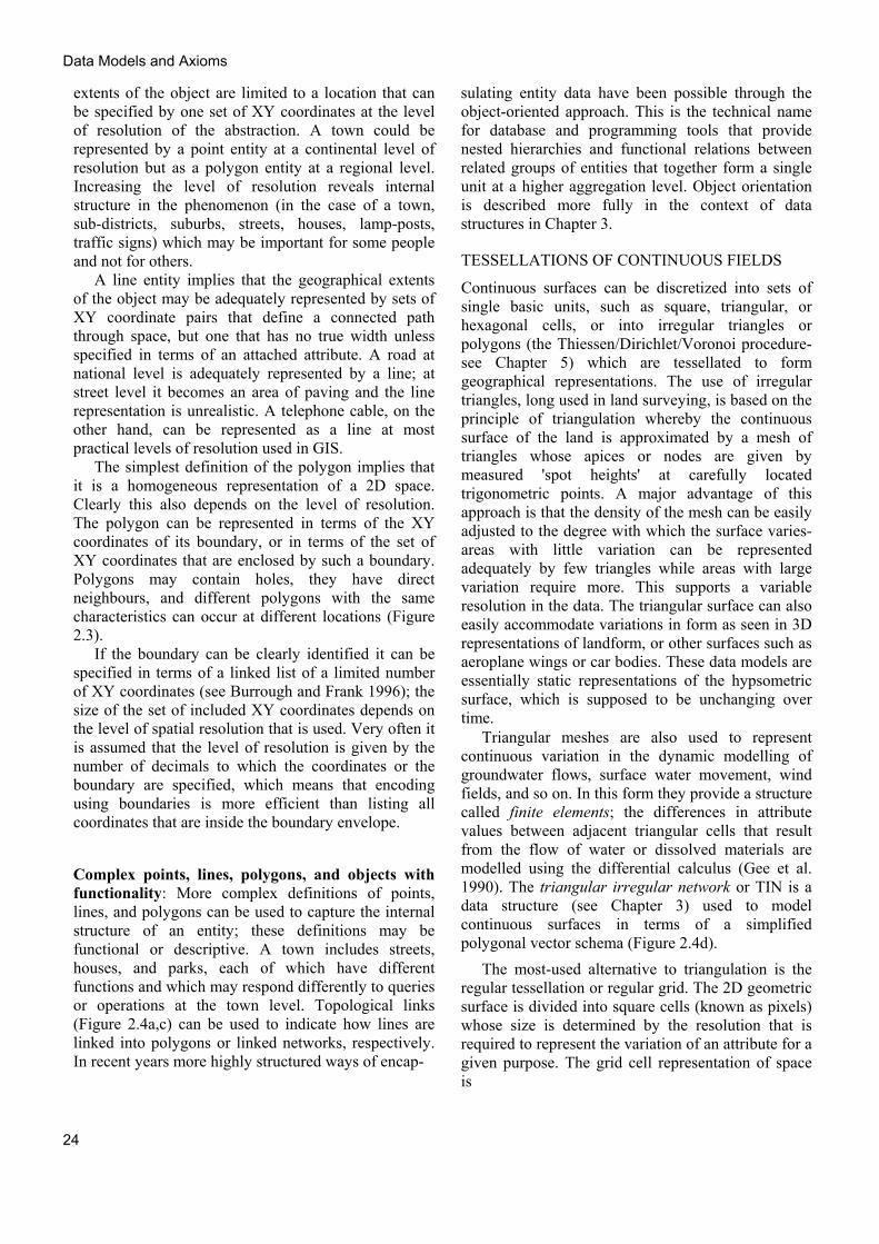
Consider now what might happen if there are disagreements about how to classify land cover. Different people or organizations might have different reasons for allocating land to different classes; even if the same number of classes are used and the central concepts of the classes are similar. Table 2.3 presents some examples of how different the results can be. Clearly, any analyses based on data from the different sources would give considerably different results, with serious implications for interpretation.

Now consider the effects of the method of survey on the results. If we collect land cover data by sam-

30


Table 2.3. Examples of vartation in estimation of land cover in Europe - km2*1000 Land use classification

FAO-Agrostat Pan-European Questionnarire by Eurostat

10 minutes Pan-European Pan Use Database

Land Use Statistical Database

Land Use Vector Database

Permanent crops Germany France Netherlands UK Forest Germany France Netherlands UK

4.42 12.11 0.29 0.51 103.84 147.84 3.00 23.64

- - - - 103.84 148.10 3.30 24.00

1.80 12.07 0.22 0.52 98.56 140.675 1.48 18.96

2.30 12.18 0.34 0.59 - 145.81 3.00 14.29

5.36 31.45 1.07 6.54 100.46 79.63 0.78 10.03

Source: RIVM 1994

pling, i.e. by visiting a set of data points on the ground and recording what is there we will have to interpolate from these 'ground truth' data to all sites where no observations have been made. The allocation of an unsampled site to a given class is then a function of the quality and density of the data and the power of the technique used for interpolation. Note that if we decide to interpolate to crisply delineated areas of land we still use the choropleth model based on the geographical primitive area/polygon. If we interpolate to a discretized surface such as a regular grid then the land cover map consists of sets of pixels with attributes indicating the land cover class to which they belong.

If we use remotely sensed data to identify land cover we automatically work with a gridded discretization of continuous space because that is how the satellite scanner works. The resolution of our spatial information is limited by the spatial resolution of the scanner, which for digital orthophotos may be very fine indeed (Plate I). Unlike the case with sampling, we do have complete cover of the area (excluding problems with cloud cover on the image and so on) so the information present in each pixel is of equal quality, which is not the case with interpolation. The major problem with identifying land cover with remotely sensed data is to convert the measurements of reflected radiation for each pixel into a prediction that a given land cover class dominates that cell. Obviously the success of the quality of the data depends on the quality of the classification process.

This example shows that two different, but complementary data models can be used for land cover mapping. The representation of these models as vectors or rasters depends partly on how the data have been collected and partly on the way they will be used.

SOIL MAPS Most published soil maps use the entity data model based on the vector polygon as the geographical primitive. Polygons are defined in terms of their soil class, which by implication is homogeneous over the unit. Boundaries are represented as infinitely thin lines implying abrupt changes of soil over very short distances. Note that inclusion of polygons in polygons is an important aspect of soil and geological maps.

This data model is practical, because it means that simply by locating a site on a map and determining the mapping unit one can retrieve information on the soil properties by consulting the survey report. However, the paradigm is scientifically inadequate because it ignores spatial variation in both soil forming processes and in the resulting soils (see Plates 4.4, 4.6). The model is conceptually identical to that used in other polygon-based spatial information, such as parcel-based land use or land ownership data, and it has provided the role model for the development of soil information systems and GIS in the late 1970s and 1980s (Burrough 1991b). Data types used to record attribute data will include nominal, integer, and real.

31


A critical aspect of delineating soil classes in geographical space concerns the interpretation of boundaries on the ground. Important soil differences may be indicated by abrupt, clearly observable physiographic features such as changes in lithology, drainage, or breaks of slope, which we can call 'primary boundaries'. However, the drawn soil boundaries may also merely reflect interpreted differences in soil classification in the data space. These we term 'secondary boundaries'.

As far as the user is concerned, printed (and digitized) soil maps do not distinguish between 'real' primary boundaries that have a physiographic basis, and 'interpreted' secondary boundaries. Consequently, as both types of boundary are represented as supposedly infinitely thin lines, the mapping procedures lead inevitably to a 'double crisp' conceptual model of soil variation, both with respect to the classification in attribute space and the geographical delineation of mapping units. According to this Boolean model any site can belong to a only single soil unit: both in attribute space and geographical space the membership of a site in soil class i is either 0 (not a member or outside the area) or 1 (is a member or is inside).

A major problem with soil, vegetation, and other similar natural phenomena, is that they vary spatially at all scales from millimetres to whole continents. Although soil scientists have long recognized this, soil cartographers still use the choropleth model for mapping soil at different levels of resolution. This generates a serious logical fallacy because at one level it assumes within-unit homogeneity, while at another spatially coherent differences in soil have been recognized. In addition, whereas with land cover we might expect the boundaries of land cover classes to be reasonably sharp and discrete because their location is often dictated by differences in human use of landscape, real soil boundaries can be sharp, gradual, or diffuse.

An alternative to the discrete polygon data model for soil is to assume that soil properties vary gradually over the landscape. The soil is sampled at a series of locations and attributes are determined for these samples. The simplest data model is then the geographical point (to represent the locations) with the values of the associated attributes. From this simple data model new data models of continuous spatial variation may be created by interpolation. The data models for describing soil as a continuous variable are, in principle, very similar to those used for the hypsometric surface of land elevation. Sets of discrete contour lines can be used to link

zones of equal attribute values, or attribute values may be interpolated to cells or locations on a regular grid, which leads to the raster model of space. As with soil and many other attributes of the physical, chemical, and biological landscape, these cannot be seen directly but must be collected at sets of sample points according to some approved sampling scheme. Both the area (or volume) of the samples (known technically as the support) and their density in space relative to the spatial variation of the attribute concerned are important for the quality of the resulting interpolations. The details of interpolation and the differences in results obtained using different methods are explained in Chapters 5 and 6.

HYDROLOGY

Hydrological applications require the modelling of the transport of water and materials over space and time, which can require changes to be signalled in attributes, and in location and form of critical patterns (e.g. water bodies). Not only may water levels in rivers, reservoirs, and lakes change but the geometry and location of water bodies can vary as well. A change in water level in a lake causes the location of the boundary between water and land to change. A flood may result in the opening up of new channels and the abandonment of old ones, thereby changing both topology and location. The simple entity vector data model of points, lines, and areas is not very well suited to dealing with hydrological phenomena because changes in geometry mean changing the coordinate and topological data in polygon networks, which can involve considerable computation. Better is to use a data model based on ideas of 'object orientation' in which primitive entities are linked together in functional groups (McDonnell 1996). The internal structure of the data model permits action on one component of the group to be passed automatically to other parts; consequently the data model contains not only geographical location, geometry, topology, and attributes but also information on how all these react to change.

Transport of material can also be easily captured by data models of continuous variation. The use of the variable resolution triangular or square finite element net is common in hydrological models but not in commercial GIS (e.g. McDonald and Harbaugh 1988). Transport of material over a surface can also be dealt with using the raster data model of continuous variation to which the surface topology has been added or derived by computation (see Chapter 8).

32


Summary: entities or fields?

Figure 2.5 summarizes the steps that need to be taken when going from a perception of reality to a set of data models that can be used in a computerized information system. In some applications the decision to opt for an entity-based approach or a field-based approach may be clear-cut. In others it may be a matter of opinion depending on the aims of the user.

Interconversion between an entity-based vector or raster representation and a continuous representation is technically possible if the original phenomena have been clearly identified. Raster-Vector conversion is covered in Chapter 4. No amount of technology, however, can make up for differences in interpretation that are made before the phenomena are recorded. If scientist X perceives the landscape as being made up of sets of crisp entities represented by polygons, his view of the world is functionally different from scientist Y, who prefers to think in terms of continuous variation. Both approaches may be distortions of a complex reality which cannot be described completely by either model.

Figure 2.2 illustrates how the preferred choice of entities or continuous fields may vary between applications and within disciplines. Generally speaking, those disciplines concerned with the inventory and recording of static aspects of the landscape opt for the entity approach; disciplines dealing with the studies of pattern and process requiring dynamic data models opt for continuous, differentiable fields.

In most GIS all locational data and attribute values are deemed to be exact. Everything is supposed to be known, there is no room for uncertainty. Very often this comes not because we are unable to cope with statistical uncertainty, but rather because it costs too much to collect or process the data needed to give us the information about the error bands that should be associated with each attribute for each data unit. But, in principle there is no reason why information on quality cannot be added to the data.

In essence, the intellectual level of the simple crisp entity models of spatial phenomena is little different from that of children's plastic building blocks. These toys obey the basic axioms of information systems, including that which says that it is possible to create a wide variety (possibly an infinite variety?) of derived objects by combining various blocks in different ways. Logically this is no different from combining sets of

points, lines, and areas from a GIS to make a new map. Given enough bricks one can build houses, recreate landscapes, or even construct life-sized models of animals like giraffes and elephants.

And this is the point. The giraffe built out of plastic blocks can be the size, the colour, and the shape of a real giraffe, but the model does not, and cannot have the functions of a giraffe. It cannot walk, eat, sleep, procreate, or breathe because the basic units of which it is built (the blocks or database elements) are not capable of supporting these functions. While this is a trivial example, the same point can be made for many database units that are used to supply geographical data to drive analytical or process oriented models. No amount of data processing can provide true functionality unless the basic units of the data models have been properly selected.

NINE FACTORS TO CONSIDER WHEN EMBARKING ON SPATIAL ANALYSIS WITH A GIS

The following nine, not necessarily independent, questions concerning spatial data are of fundamental importance when choosing data models, and database approaches for any given application:

1. Is the real world situation/phenomena under study simple or complex?

2. Are the kinds of entities used to describe the situation/phenomena detailed or generalized?

3. Is the data type used to record attributes Boolean, nominal, ordinal, integer, real, or topological?

4. Do the entities in the database represent objects that can be described exactly, or are these objects complex and possibly somewhat vague? Are their properties exact, deterministic, or stochastic?

5. Do the database entities represent discrete physical things or continuous fields?

6. Are the attributes of database entities obtained by complete enumeration or by sampling?

7. Will the database be used for descriptive, administrative, or analytical purposes?

8. Will the users require logical, empirical, or process-based models to derive new information from the database and hence make inferences about the real world?

9. Is the process under consideration static or dynamic?

33


Questions 1. Develop simple data models for use in the following applications:

A road transport information system The location of fast food restaurants The incidence of landslides in mountainous terrain The dispersion of pollutants in groundwater An emergency unit (police, fire, ambulance) A tourist information system The monitoring of vegetation change in upland areas The monitoring of movement of airborne pollutants, such as the 137CS deposited by rain from the

Chernobyl accident in 1986. Consider the sources of data, the kinds of phenomena being represented, the data models, the data types, and the main requirements of the users.

Suggestions for further reading

COUCLELIS, H. (1992). People manipulate objects (but cultivate fields): beyond the raster-vector debate in GIS. In A. U. Frank, I. Campari, and u. Formentini ( eds. ), Theories and Methods of Spatio- Temporal Reasoning in Geographic Space. Springer Verlag, Berlin, pp. 65-77.

GAHEGAN, M. ( 1996) .Specifying the transformations within and between geographic data models. Transactions in GIS, 1: 137-52. GATRELL, A. C. (1991). Concepts of Space and Geographical Data. In D. J. Maguire, M. F. Goodchild, and D. W. Rhind (eds.),

Geographical Information Systems: Principles and Applications, vol. ii, Longman Scientific and Technical, Harlow, pp.119-34. HARVEY, D. (1969). Explanation in Geography. Edward Arnold, London.

34

Principles of Geographical Information Systems

Documents

Transcript of Principles of Geographical Information Systems