Principles and models for the Embedded Value calculation · Principles and models for the Embedded...

Trieste – February 2012

Principles and models for the Embedded Value calculation

2 AGENDA

1. Methodological Aspects: from the Traditional to the Market

Consistent Embedded Value

2. CFO Principles: the MCEV framework

3. Stochastic scenarios: calibration and validation

4. Asset and Liabilities valuation: looking for a consistent approach

through the risk free definition

5. The MCEV calculation: a simple and “practical” example

3 AGENDA

Limits of traditional Embedded Value

CFO Forum and EEV Principles

Getting to grips with Embedded Value

Basic definitions: Embedded Value

Why not just using the Balance Sheet?

Value of in-force business (VIF)

From Traditional to Market Consistent EV

Market Consistent Embedded Value

Traditional EV: technical aspects



4 AGENDA












5 Life business: characteristics

Characteristics of life business:

• long duration of contracts

• uncertain payments to policyholders (“if”, “when” and “how much”)

• presence of guarantees for policyholders

– minimum death benefits

– minimum guaranteed rates

• dependence on economic variables (“financial”)

– interest rates, equity returns

– inflation

• dependence on operating variables (“non financial”)

– mortality

– lapses

– expenses

• dependence on accounting practices

– deferred acquisition costs

– local / IFRS accounting


6 Measuring the value from a SH’s perspective


ASSETS

What is the Balance Sheet missing to recognise?

NAV

Realistic

liabilities

UGLs

LIABILITIES

Solvency

Capital

Excess

Capital

The difference between MV and BV

of assets:

• UGLs on Assets backing NAV

• UGLs on Assets backing Liabilities

• Split of UGLs between SHs and PHs

The prudent basis used in pricing

and reserving:

• intrinsic value in the reserves

The use of SH’s capital (and the fact

taxes are to be paid on it), which

must be remunerated:

• cost of holding a (regulatory or

internally determined) solvency capital

7

P&L result is not necessarily a valid indicator of value creation, e.g.:

1. P&L high profit but value destruction

• High lapses in one year bring high profits due to surrender penalties, but…

• Loss of stream of future profits expected from the contracts that lapsed is

higher than the profit of the year;

2. P&L loss but value creation

• High new business volumes in one year bring high acquisition expenses

with consequent losses, but…

• Stream of future profits expected from the new contracts is higher than the

loss of the year

Measuring the value from a SH’s perspective

What is the P&L missing to recognise?


8

Premiums are not necessarily a valid indicator of value creation:

• low volumes – high margins

• high volumes – low margins

• duration of contracts

low surrender penalties – high surrenders

high surrender penalties – low surrenders

• financial options and g’tees

• solvency requirement

It is the VALUE of the PREMIUMS that actually matters, taking into

account the cost of the solvency margin

Measuring the value from a SH’s perspective

What is the P&L missing to recognise?


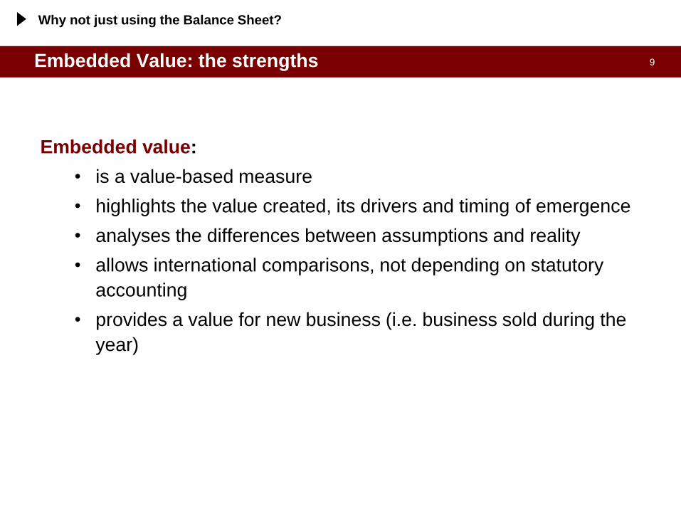
9 Embedded Value: the strengths


Embedded value:

• is a value-based measure

• highlights the value created, its drivers and timing of emergence

• analyses the differences between assumptions and reality

• allows international comparisons, not depending on statutory

accounting

• provides a value for new business (i.e. business sold during the

year)

10 AGENDA












11

ANAV

(Adjusted Net

Asset Value) EMBEDDED

VALUE

Balance Sheet

VIF

(Value In-Force) LIABILITIES

ASSETS

NAV

Value of a life insurance company

Basic definitions: Embedded Value and Appraisal Value

12

ANAV

(Adjusted Net

Asset Value)

DEFINITION:

Company’s published net assets adjusted to reflect the market value of the

related backing assets

ANAV is equal to the sum of:

• Net Asset Value (shareholders’ equity)

• adjustments to Net Asset Value (after taxes and PH participation)

- unrealised gains and losses (+/-)

- intangibles (start up costs, Deferred Acquisition Costs, …) (-)

- revaluation of participated companies (+)

- cross participations (-)

Adjusted net asset value


13

VIF

(Value In-

Force)

DEFINITION:

Present value at valuation date of future industrial profits (after taxes and reinsurance) expected to emerge from all contracts existing at valuation date, after allowance for the cost of financial guarantees and options, the cost of non financial risks and the cost of holding the required capital

Value of in-force (VIF)

value “implicit” in the contracts already in-force


14 AGENDA












15 Traditional VIF


GENERAL VIF DEFINITION:

Present value at valuation date of future industrial profits (after taxes and reinsurance) expected to emerge from all contracts existing at valuation date, after allowance for the cost of financial guarantees and options, the cost of non financial risks and the cost of holding the required capital

To be noted:

under TEV approach, the cost of financial guarantees and options and the cost of non financial risks are not taken into account explicitly (but only implicitly within the discount rate)

16 Traditional VIF definition

TRADITIONAL VIF DEFINITION:

Present value, at valuation date, of future industrial profits (after taxes and

reinsurance) expected to emerge from all contracts existing at valuation date,

taking into account the cost of holding the capital


VIF = PVFP - CoC

PVFP = Σt Ut

(1 + r)t

where

Ut = industrial profit (after tax and reinsurance)

r = discount rate

CoC = Σt

where

Ct-1 = capital

i = return on assets backing the capital

r = discount rate

Ct-1 * [r – i * (1 – tax)]

(1 + r)t

17 PVFP calculation: main aspects

PVFP: Present value of future industrial profits, after taxes and reinsurance

INDUSTRIAL PROFITS: technical profits + financial profits

• technical profits: mortality profits + surrender profits + loading profits

• financial profits: investment income - technical interests (i.e. minimum

guaranteed + revaluations)

How to calculate the PVFP

Database Future Assumptions

Other Issues

− Economic assumptions:

− Investment returns

− taxation rate

− Operating assumptions:

− Lapses

− Mortality

− Maintenance Expenses

− Discount Rate

− Impact of DAC

− Reinsurance

− Contingency Reserves

− Info regarding all the policies in the

portfolio at valuation date


18 Projection of future profits: demographic analysis


Demographic Analysis Gross Profit and Loss Account

Policies fully First Surrender Maturity Paid-Up Paid-Up Paid-Up Paid-Up Paid-Up

Year in force Elimination New in force Elimination Surrender Maturity

2010 786,319 1,484 24,560 34,750 7,082 - 5 46 36

2011 718,444 1,407 20,392 29,309 7,305 6,995 15 183 170

2012 660,030 1,337 17,268 30,859 7,038 13,932 26 317 320

2013 603,528 1,247 15,203 30,647 6,348 20,307 36 431 512

2014 550,084 1,152 13,309 34,709 5,278 25,675 45 508 794

2015 495,636 1,076 11,577 28,305 4,067 29,606 51 545 1,101

2016 450,611 1,025 10,088 28,195 3,151 31,976 56 545 1,313

2017 408,151 966 8,731 31,497 2,405 33,213 59 520 1,608

2018 364,553 903 7,434 27,472 1,861 33,431 61 481 1,586

2019 326,882 859 6,250 28,302 1,437 33,165 62 422 2,004

2020 290,033 817 5,128 27,443 1,098 32,114 61 354 2,360

2021 255,548 779 4,354 27,115 830 30,437 60 278 2,743

2022 222,470 734 3,805 27,788 612 28,185 57 208 3,296

… … … … … … … … … …

2041 2,409 72 9 - - - - - -

2042 2,329 76 8 - - - - - -

2043 2,244 46 5 1,488 - - - - -

2044 706 10 1 695 - - - - -

- - - - - - - - -

19 Projection of future profits: P&L account


Gross Profit and Loss Account

Premiums Reserves Investment Reserves Payments Commissions Expenses Gross

Year Incoming Income Outgoing Result

1,384

2010 709 6,109 266 6,327 556 1 28 172

2011 660 6,327 280 6,510 557 1 27 172

2012 612 6,510 292 6,610 610 1 25 167

2013 566 6,610 301 6,655 634 1 24 163

2014 520 6,655 299 6,569 728 1 22 153

2015 474 6,569 333 6,487 693 1 21 175

2016 431 6,487 327 6,351 716 1 19 159

2017 389 6,351 318 6,115 777 1 18 148

2018 350 6,115 305 5,862 754 1 16 136

2019 312 5,862 291 5,539 786 1 15 125

2020 275 5,539 272 5,168 791 1 14 113

2021 239 5,168 253 4,760 787 1 12 101

2022 205 4,760 231 4,299 796 1 11 89

… … … … … … … … …

2041 3 189 11 193 7 - 0 3

2042 3 193 11 196 7 - 0 4

2043 1 196 6 36 164 - 0 2

2044 - 36 1 - 37 - 0 0

- - - - - - - -

20 Projection of future profits: from gross to industrial results


Gross Profit and Loss Account PVFP Portfolio Value Breakdown

UIt

Gross Reinsurance Before Tax Taxation Industrial

Result Result Industrial Profit Profit

1,384 - 343 1,042 398 643

172 - 36 136 52- 84

172 - 46 126 48- 78

167 - 43 125 48- 77

163 - 40 123 47- 76

153 - 37 116 44- 72

175 - 48 127 49- 78

159 - 43 116 44- 72

148 - 39 108 41- 67

136 - 36 100 38- 62

125 - 33 92 35- 57

113 - 29 84 32- 52

101 - 25 76 29- 47

89 - 22 68 26- 42

… … … … …

3 - 3 1- 2

4 - 4 1- 2

2 - 2 1- 1

0 - 0 0- 0

- - - - -

21

n

i

i

irxPV

1

)1(

Profit 84 78 77 76 72 …

Time YE09 YE10 YE11 YE12 YE13 YE14 …

x1 x2 x3 x4 x5 x6

0 1 2 3 4 5 6

r: discount rate

643...58626878...%)25.71(

76

%)25.71(

77

%)25.71(

78

%)25.71(

84

432PVFP

r=7.25%

Present value of future profits (PVFP)


Portfolio Value Breakdown

UIt

Industrial

Year Profit

643

2010 84

2011 78

2012 77

2013 76

2014 72

2015 78

2016 72

2017 67

2018 62

2019 57

2020 52

2021 47

2022 42

… …

2041 2

2042 2

2043 1

2044 0

-

22 AGENDA












23

Financial

Demographic

Expenses

Taxation

“Best Estimate” assumptions

• determined by each Company at the

valuation date, having regard to past,

current and expected future

experience and to any other relevant

data

• set within the context of a going

concern (i.e. new business will

continue to be written)

Future projections: assumptions


24

RISK FREE (10-y AAA Government bond)

GOVERNMENT BONDS (risk free*)

CORPORATE BONDS

(risk free + spread(1) for liquidity premium)

EQUITIES (risk free + spread(2))

PROPERTIES (risk free + spread(3))

Long term Future Investment Return

Asset Mix backing

mathematical reserves

(equities, properties,

corporate bonds,

government bonds…)

Risk Discount Rate (RDR)

risk free + Spread(4)

Future projections: financial assumptions


UGLs on equities

(assumed realisation: 5 years)

UGLs on properties

(assumed realisation: whole projections)

UGLs on bonds

(assumed realisation: duration)

Future Investment Return

(UGLs included)

25

Best-estimate economic assumptions as at 31 December 2009

Italy Germany France CEE RoE RoW

10 y Government Bond 4.02% 3.44% 3.57% 4.55% 3.46% 5.54%

Equity Total Return 6.34% 6.34% 6.34% 6.51% 6.11% 8.03%

Property Total Return 4.59% 4.59% 4.59% 5.41% 3.77% 6.13%

Return on Equities= spread 2.90%

Return on Properties = spread 1.15%

Return on Equities= spread 2.90% on AAA but 2.32% on local govt

Return on Property= spread 1.15% on AAA but 0.57% on local govt



Source: Generali – Life Embedded Value 2009 – Supplementary Information

Example: Generali

26

A RISK PREMIUM IS REQUIRED

BY THE SHAREHOLDER

- if the future profits are certain risk free

- insurance business uncertain

- shareholders want to pay less for uncertain businesses

Risk, apparently ignored in a deterministic traditional approach, is instead

already taken into account via a discount rate higher than the risk free rate:

risk free + risk premium.

But how was the risk premium calculated?


The discount rate is the return offered to a shareholder on his investment in

the company


27

The risk premium:

- should depend on the company riskiness

- should depend on the line of business

- should be different between VIF, ANAV and Goodwill

but…

- in the traditional deterministic approach it is not determined on a scientific basis, but based on market practice (range between 2.5%-4.0%)

- it is typically set equal to the equity risk premium

- same risks could be valued differently depending on the prudentiality of the company



28

• Mortality: Company experience, where available

• Surrenders: Company experience, where available

• If not available? Market experience with possible prudential corrections

Demographic assumptions


Further difficulties in setting demographic assumptions when:

• data on past experience is unavailable/insufficient for a specific product;

• rates experienced in the past years are not deemed to be valid as long term

assumptions (especially for surrenders rates, which strongly depend on the

economic environment)

29

Cost of Capital:

Cost/Loss of interest due to holding the capital

Annual cost:

r: shareholders’ required rate of return

i * (1 – tax)

shareholder actual return from

investing Ci in an insurance company

Cost of capital


Ci * [r – i * (1 – tax)]

Within TEV valuation, the amount of capital (C) is typically set equal to the level

of minimum solvency margin

i: return of assets backing the capital

(gross of taxes)

30 Cost of capital


PVFP - CoC formula Portfolio Value Breakdown

CoC Ct * r Ct * i * (1-tax) PVFP - CoCCost of Required Return After Tax Return Industrial Profit

Solvency Margin on Solvency Margin on Solvency Margin after Cost of SM

55 148 93 588

6 16 10 78

6 17 10 72

6 17 11 71

6 17 11 70

6 17 11 65

6 17 10 72

6 16 10 65

6 16 10 61

6 15 9 56

5 14 9 52

5 13 8 47

5 12 8 42

4 11 7 37

… … … …

0 0 0 2

0 0 0 2

0 0 0 1

0 0 0 0

- - - -

31 AGENDA












32

1. Subjective choice of Risk Discount Rate (RDR)

2. Subjective choice of financial assumptions

3. Indirect allowance for financial guarantees

4. Capitalisation of asset risk premium

Technical limits

TEV methodology: technical limits

Limits of Traditional Embedded Value

33

RDR should reflect

• shareholder’s expected return

• level of risk in the business at each valuation date

Risk Margin in RDR is NOT actively linked to risk

• it usually reflects market practice

• use of similar risk margins between companies rather than active

differentiation on the basis of the risks being run (“herding” tendency)

TEV methodology: 1) subjective choice of RDR


34

BOND return: 5%

EQUITY return: 7.5%

Risk Discount Rate: 7.5%

21.86 €

23.50 €

2,000 €

5.87%

35% Equities, 65% Bonds

94.00 €

PVFP:

SH Interest:

Reserves:

Expected Return:

Asset Mix:

PH Interest:

23.49 €

25.60 €

2,000 €

6.40%


102.40 €

COMPANY A COMPANY B

BOND return: 5%

EQUITY return: 9%

Risk Discount Rate: 9%

Example n°1: Capitalisation product with profit sharing = 80% of financial result

Company A and B: same asset mix but different financial assumptions

the higher the financial assumptions, the higher the value

TEV methodology: 2) subjective choice of financial assumptions


35

Traditional VIF calculation

• explicitly captures the value of “in the money” guarantees to the

extent that they have impact on projected profits (Intrinsic Value)

• implicitly allows, in the RDR, for the possibility that guarantees move

(further) into the money (Implicit allowance for Time Value of FG)

TEV methodology: 3) indirect allowance for financial guarantees


36


Company A and B: same asset mix and financial assumptions but different guarantee for PH

TEV methodology: 3) indirect allowance for financial guarantees

21.86 €

23.50 €

2,000 €

5.87%


94.00 €

PVFP:

SH Interest:

Reserves:

Expected Return:

Asset Mix:

PH Interest:

21.86 €

23.50 €

2,000 €

5.87%


94.00 €

COMPANY A

Guarantee: none

COMPANY B

Guarantee: 3%

Same value for companies running different risks

When best estimate assumptions are higher than guarantees, the cost of financial

guarantees is not explicitly captured

BOND Return: 5%, EQUITY Return: 7.5%, Risk Discount Rate: 7.5%


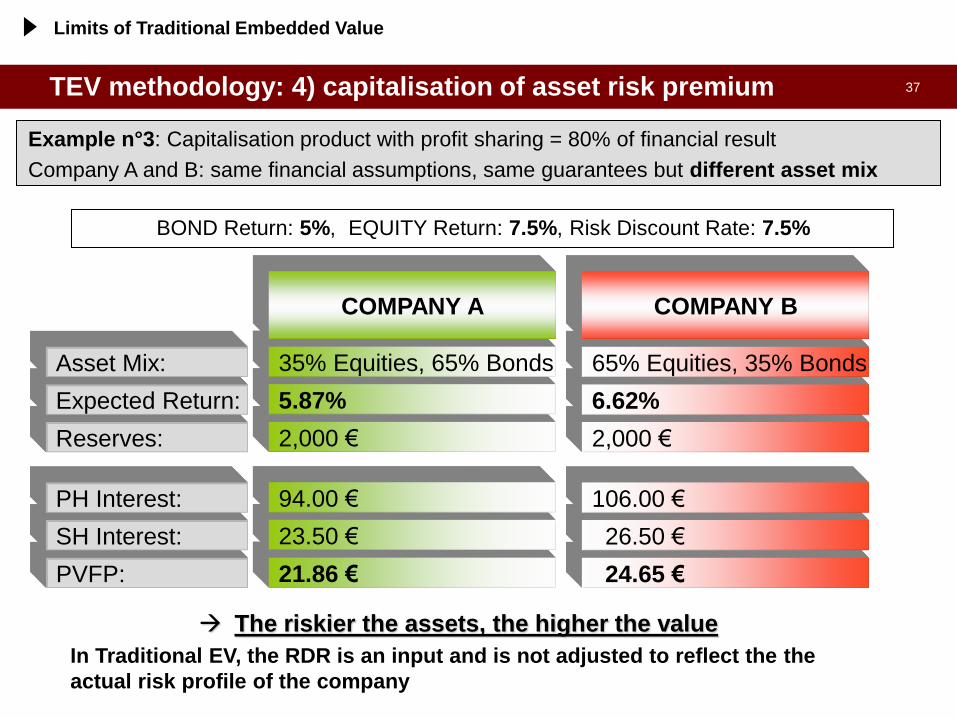
37 TEV methodology: 4) capitalisation of asset risk premium


Company A and B: same financial assumptions, same guarantees but different asset mix

21.86 €

23.50 €

2,000 €

5.87%


94.00 €

PVFP:

SH Interest:

Reserves:

Expected Return:

The riskier the assets, the higher the value

In Traditional EV, the RDR is an input and is not adjusted to reflect the the

actual risk profile of the company

Asset Mix:

PH Interest:

24.65 €

26.50 €

2,000 €

6.62%


106.00 €

COMPANY A COMPANY B

BOND Return: 5%, EQUITY Return: 7.5%, Risk Discount Rate: 7.5%


38

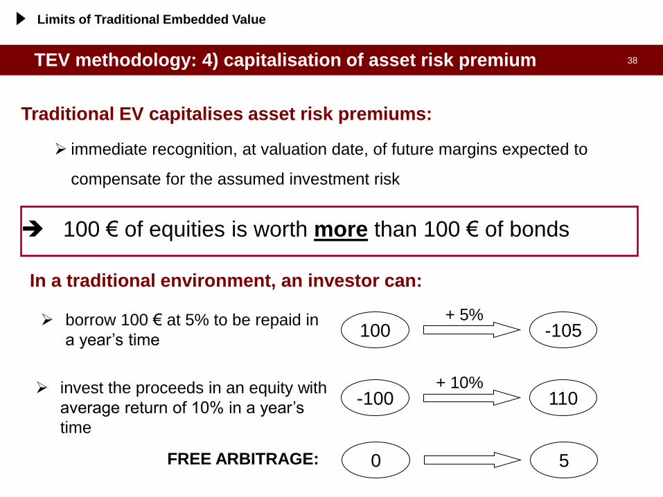
100 € of equities is worth more than 100 € of bonds

Traditional EV capitalises asset risk premiums:

immediate recognition, at valuation date, of future margins expected to

compensate for the assumed investment risk

In a traditional environment, an investor can:

borrow 100 € at 5% to be repaid in

a year’s time

invest the proceeds in an equity with

average return of 10% in a year’s

time

-105 100 + 5%

110 -100 + 10%

FREE ARBITRAGE: 5 0

TEV methodology: 4) capitalisation of asset risk premium


39 AGENDA












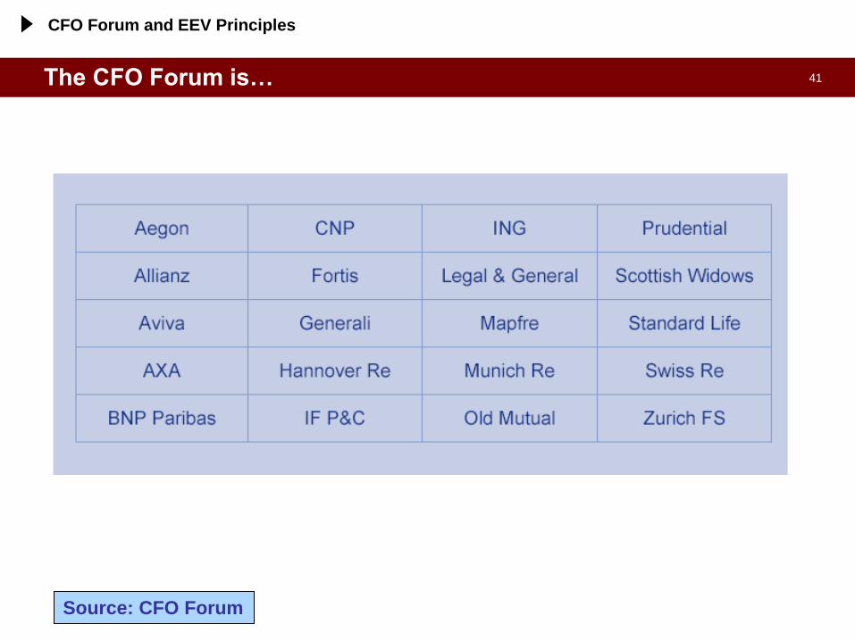
40 The CFO Forum is…

a high level discussion group

founded in 2002

focused on:

• new regulations for insurers

• increase in transparency for investors

• improving consistency of information

reported

with wide representation from major

European-centred insurance groups



Source: CFO Forum


42

In May 2004, the CFO Forum published the

European Embedded Value Principles and

member companies agreed to adopt EEVP

from 2006 (with reference to 2005 financial

year)

EEV Principles consisted of 12 Principles and

65 related areas of Guidance

Other 127 comments, collected in the “Basis

for Conclusions”, summarised the

considerations in producing the Principles and

Guidance

In October 2005, additional guidance on EEV

disclosures was published to improve

consistency of disclosures and sensitivities



43 CFO Forum and EEV Principles

European Embedded Value Principles

Principle 1 Introduction

Principle 2 Coverage

Principle 3 EV Definitions

Principle 4 Free Surplus

Principle 5 Required capital

Principle 6 Future shareholder cash flow

from the in-force covered

business

Principle 7 Financial options and

guarantees

Principle 8 New Business and renewals

Principle 9 Assessment of appropriate

projection assumptions

Principle 10 Economic assumptions

Principle 11 Participating business

Principle 12 Disclosure


required use of stochastic simulations

to determine impact of financial

guarantees

44

Return SH's result 0.0% -3.0%

0.5% -2.5%

1.0% -2.0%

1.5% -1.5%

2.0% -1.0%

2.5% -0.5%

3.0% 0.0%

3.5% 0.5%

4.0% 1.0%

4.5% 1.0%

5.0% 1.0%

5.5% 1.0%

6.0% 1.0%

6.5% 1.0%

7.0% 1.0%

7.5% 1.0%

8.0% 1.0%

8.5% 1.0%

9.0% 1.0%

9.5% 1.0%

10.0% 1.0%

10.5% 1.1%

11.0% 1.1%

11.5% 1.2%

12.0% 1.2%

12.5% 1.3%

13.0% 1.3%

13.5% 1.4%

14.0% 1.4%

14.5% 1.5%

15.0% 1.5%

Asymmetry of SH’s results:

the mean SH’s result is lower than the SH’s result in the mean scenario

PH's result = max (gar, min (return*a, return - fee)

SH's result = return - PH's result

-3.5%

-3.0%

-2.5%

-2.0%

-1.5%

-1.0%

-0.5%

0.0%

0.5%

1.0%

1.5%

2.0%

0.0% 2.0% 4.0% 6.0% 8.0% 10.0% 12.0% 14.0% 16.0%

Fund return

SH

's r

es

ult

Guaranteed interest (gar) 3%

Participation percentage (a) 90%

Minimum retained (fee) 1%

The financial asymmetry of SH’s result

45

• Insurance business is asymmetric:

– in “positive” scenarios, SHs earn only a share of the financial profit

(due to the profit sharing with PHs)

– in “negative” scenarios, SHs bear the full cost

(due to the presence of guaranteed interests)

the mean of PVFPs is lower than the PVFP of the mean scenario

To capture the financial asymmetry (i.e. volatility of financial parameters):

• TEV

– 1 single scenario (“Best Estimate”)

– implicit allowance for risks within the discount rate (290bps over govt.bonds)

• STOCHASTIC APPROACH:

– a number of stochastic scenarios is considered (1000 or 5000 or …)

– in each scenario future profits and PVFP are calculated

– the final PVFP is the mean of all the PVFPs in the stochastic scenarios

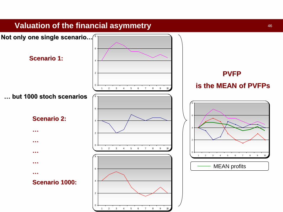
Valuation of the financial asymmetry

46

Not only one single scenario…

Scenario 1:

… but 1000 stoch scenarios

Scenario 2:

…

…

…

…

…

Scenario 1000:

0

2

4

6

8

1 2 3 4 5 6 7 8 9 10

0

2

4

6

8

1 2 3 4 5 6 7 8 9 10

0

2

4

6

8

1 2 3 4 5 6 7 8 9 10

PVFP

is the MEAN of PVFPs

0

2

4

6

8

1 2 3 4 5 6 7 8 9 10

MEAN profits

Valuation of the financial asymmetry

47 AGENDA












48 Market Consistent Embedded Value

Stochastic approach, consistent with modern financial theory

Avoid subjectivity in the choice of RDR and financial assumptions

Avoid capitalisation of asset risk premium (no arbitrage)

Impact of financial guarantees is captured in all possible scenarios

(no implicit allowance)

Two main possible approaches leading to same results

Deflator approach

Risk-neutral approach

Market consistent valuation:

all projected cash flows are valued in line with the prices of similar

cash flows that are traded in the financial market


49 MCEV: two different approaches

Two possible ways to reflect Risk Aversion:

using real-world probabilities of scenarios and calibrating to the

market scenario dependent discount rates (Deflator approach)

discounting at the risk-free rate and calibrating to the market

probabilities of scenarios (Risk-neutral approach)

Equity Price = P0 Scenario1: Equity Price = P1

Scenario2: Equity Price = P2

2

22

1

11

01

*

1

*

discount

yprobabilitP

discount

yprobabilitPP


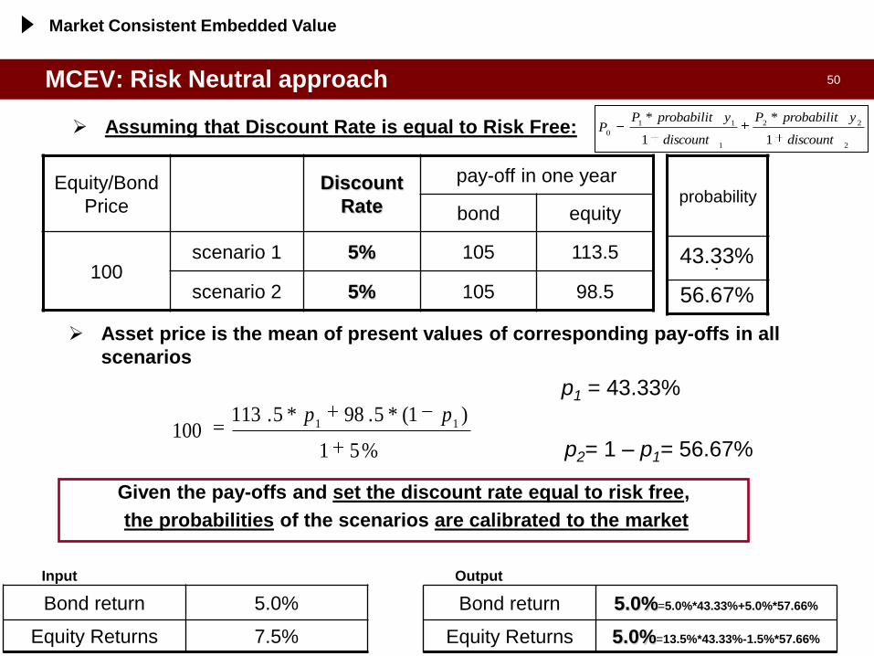
50

?

probability

MCEV: Risk Neutral approach

Assuming that Discount Rate is equal to Risk Free:

Asset price is the mean of present values of corresponding pay-offs in all

scenarios

Given the pay-offs and set the discount rate equal to risk free,

the probabilities of the scenarios are calibrated to the market

p1 = 43.33%

p2= 1 – p1= 56.67% %51

)1(*5.98*5.113100

11pp

Equity/Bond

Price

Discount

Rate

pay-off in one year

bond equity

100 scenario 1 5% 105 113.5

scenario 2 5% 105 98.5

?

2

22

1

11

01

*

1

*

discount

yprobabilitP

discount

yprobabilitPP

Bond return 5.0%=5.0%*43.33%+5.0%*57.66%

Equity Returns 5.0%=13.5%*43.33%-1.5%*57.66%

Bond return 5.0%

Equity Returns 7.5%

Input

Output

43.33%

56.67%


51 “Certainty Equivalent”: contract with 80% financial PS, no guarantee

19.05 € 19.05 € PVFP:

10.90 € 3.10 €

31.90 € 42.10 €

Scenario 2

Scenario 1

SH Interest:

43.60 € 12.40 €

127.60 € 168.40 €

Scenario 2

Scenario 1

PH Interest:

2,000 € Reserves: 2,000 €

2.725% 0.775% Scenario 2

Scenario 1 7.975%

35% Equities

65% Bonds Expected returns:

Asset Mix:

10.525%

65% Equities

35% Bonds

COMPANY B COMPANY A

19.05 €

20 €

80 €

2,000 €

5%

Risk Free

COMPANY C

Certainty Equivalent: deterministic approach with

Risk Free as investment return / Risk free as RDR

For business where

cash flows do not

depend on, or move

linearly with market

movements

(i.e. business not

characterised by

asymmetries in

shareholder’s

results), Certainty

Equivalent

approach

is the correct choice:

Unit Linked without

guarantees

Zero coupon

Terms

Non participating

products


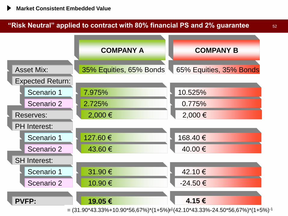
52

19.05 € 4.15 € PVFP:

10.90 € Scenario 2

Scenario 1

SH Interest:

43.60 € Scenario 2

Scenario 1

PH Interest:

2,000 € Reserves: 2,000 €

2.725% 0.775% Scenario 2

Scenario 1 7.975%


Expected Return:

“Risk Neutral” applied to contract with 80% financial PS and 2% guarantee

Asset Mix:

10.525%


COMPANY B

-24.50 €

31.90 € 42.10 €

40.00 €

127.60 € 168.40 €

COMPANY A

= (31.90*43.33%+10.90*56,67%)*(1+5%)-1 = (42.10*43.33%-24.50*56,67%)*(1+5%)-1


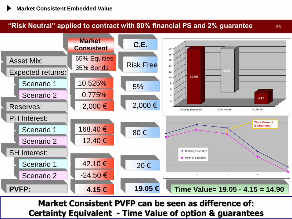
53

PVFP:

Scenario 2

Scenario 1

SH Interest:

Scenario 2

Scenario 1

PH Interest:

Reserves:

Scenario 2

Scenario 1

Expected returns:

Asset Mix:

Market Consistent PVFP can be seen as difference of: Certainty Equivalent - Time Value of option & guarantees

4.15 €

-24.50 €

42.10 €

12.40 €

168.40 €

2,000 €

0.775%

10.525%

65% Equities

35% Bonds

Market Consistent

19.05

14.90

4.15

-

2

4

6

8

10

12

14

16

18

20

Certainty Equivalent Time Value PVFP MC

1 2 3 4 5

Certanty Equivalent

Mean of Scenarios

Time Value of

Guarantees

1 2 3 4 5

Certanty Equivalent

Mean of Scenarios

Time Value of

Guarantees

“Risk Neutral” applied to contract with 80% financial PS and 2% guarantee

19.05 €

20 €

80 €

2,000 €

5%

Risk Free

C.E.

Time Value= 19.05 - 4.15 = 14.90


54 AGENDA









a high level discussion group

founded in 2002

focused on:

• new regulations for insurers

• increase in transparency for investors

• improving consistency of information

reported

with wide representation from major European-

centred insurance groups

56

In May 2004, the CFO Forum published the

European Embedded Value Principles and

member companies agreed to adopt EEVP

from 2006 (with reference to 2005 financial

year)

EEV Principles consisted of 12 Principles and

65 related areas of Guidance

Other 127 comments, collected in the “Basis

for Conclusions”, summarised the

considerations in producing the Principles and

Guidance

In October 2005, additional guidance on EEV

disclosures was published to improve

consistency of disclosures and sensitivities


57 Away from TEV: EEV Principles

European Embedded Value Principles

Principle 1 Introduction

Principle 2 Coverage

Principle 3 EV Definitions

Principle 4 Free Surplus

Principle 5 Required capital

Principle 6 Future shareholder cash flow

from the in-force covered

business

Principle 7 Financial options and

guarantees

Principle 8 New Business and renewals

Principle 9 Assessment of appropriate

projection assumptions

Principle 10 Economic assumptions

Principle 11 Participating business

Principle 12 Disclosure

Required use of appropriate approaches (e.g. stochastic simulations) to determine

the impact of financial guarantees

Generali’s first EEV disclosure in May 2006, with YE2005 results

58 EEV Principles

At the time, the EEV Principles represented a major step forward,

introducing several major improvements:

requirement for stochastic evaluation of financial guarantees and options

disclosure of sensitivities and analysis of movement

codification of several areas of current best practice, including disclosure

on methodology and assumptions used

...but different approaches were still allowed!

59

In line with the emerging move towards a market consistent embedded

value approach

TOP DOWN EEV: risk

discount rate based on

company’s WACC

MCEV: market consistent

embedded value

EEV Principles

Generali’s first MCEV disclosure in March 2008, with YE2007 results

TOP DOWN EEV

MCEV

TOP DOWN EEV

MCEV

OTHER

TOP DOWN EEV

MCEV

OTHER

TOP DOWN EEV

MCEV

OTHER

0%

20%

40%

60%

80%

100%

YE2004 YE2005 YE2006 YE2007

60 CFO Forum – June 2008: launch of MCEV Principles

On the 4th June 2008, the CFO

published the Market Consistent

Embedded Value Principles1 and

associated Basis for Conclusions

MCEV Principles:

• replaced the EEV Principles (i.e.

standalone document, not

supplement to EEV)

• at beginning compulsory from

year-end 2009 for CFO Forum

members (early adoption was

possible)

• mandated independent external

review of results as well as

methodology and assumptions

1 Copyright© Stichting CFO Forum Foundation 2008

61 MCEV Principles (June 2008)

Market Consistent Embedded Value Principles

Financial Options and

Guarantees

Principle 7

Frictional Costs of

Required Capital

Principle 8

Required Capital Principle 5

Value of in-force

Covered Business

Principle 6

Principle 9

Principle 4

Principle 3

Principle 2

Principle 1

Cost of Residual Non

Headgeable Risks

Free Surplus

MCEV Definitions

Coverage

Introduction

Financial Options and

Guarantees

Principle 7

Frictional Costs of

Required Capital

Principle 8

Required Capital Principle 5

Value of in-force

Covered Business

Principle 6

Principle 9

Principle 4

Principle 3

Principle 2

Principle 1

Cost of Residual Non

Headgeable Risks

Free Surplus

MCEV Definitions

Coverage

Introduction

Stochastic models Principle 15

Investment Returns and

Discount Rates

Principle 13

Reference Rates Principle 14

Principle 17

Principle 16

Principle 12

Principle 11

Principle 10

Disclosure

Participating business

Economic Assumptions

Assessment of Appropriate

Non Economic Projection

Assumptions

New Business and

Renewals

Stochastic models Principle 15

Investment Returns and

Discount Rates

Principle 13

Reference Rates Principle 14

Principle 17

Principle 16

Principle 12

Principle 11

Principle 10

Disclosure

Participating business

Economic Assumptions

Assessment of Appropriate

Non Economic Projection

Assumptions

New Business and

Renewals

62 MCEV Principles (June 2008): main implications

The launch of MCEV Principles was initially welcomed by analysts and investor

community and it was seen as a step in the right direction

Main implications of the MCEV Principles:

• all projected cash flows should be valued in line with the price of similar cash flows that are

traded in the capital markets [Principle 3 & 7]

• use of swap rates as reference rates (i.e. proxy for risk-free rate) [Principle 14]

• no adjustment for illiquidity premium is allowed [Principle 14]

• volatility assumptions should be based on implied volatilities derived from the market as at

the valuation date (rather than based on historic volatilities) [Principle 15]

• required capital should include amounts required to meet internal objectives (based on

internal risk assessment or targeted credit rating) [Principle 5]

• explicit and separate allowance for the cost of non hedgeable risks [Principle 9]

63

Par Rate EUR (Swap) vs Par Rate ITA (Govt) - YE2008

1.00%

2.00%

3.00%

4.00%

5.00%

6.00%

1 2 3 4 5 6 7 8 9 10 11 12 13 14 15 16 17 18 19 20 21 22 23 24 25 26 27 28 29 30

EUR (swap) ITA (govt)

Average Δ (Swap - Govt)

-0.94%

Financial market situation at YE2008: a “dislocated” market

For Italy

government bond

rates higher than

swap rates

64

VSTOXX - Implied Volatility DJ EUROSTOXX 50

0%

20%

40%

60%

80%

100%

Dec-07 Mar-08 Jun-08 Sep-08 Dec-08

VSTOXXI

Financial market situation at YE2008: a “dislocated” market

EQUITY VOLATILITY AT

HISTORICAL PEAK

CORPORATE SPREADS AT

RECORD LEVELS

JPM Maggie Overall - Maturity 5-7y - ASW Govt, bps

0

100

200

300

400

500

600

dic-07 mar-08 giu-08 set-08 dic-08

AAA AA A BBB

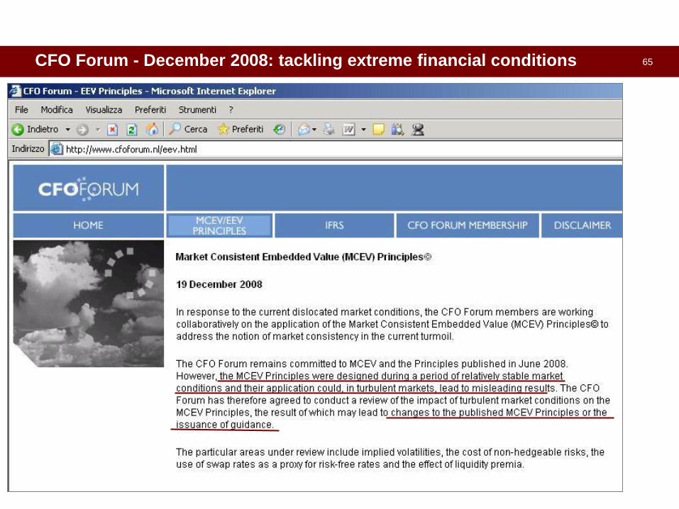
65 CFO Forum - December 2008: tackling extreme financial conditions

66 CFO Forum - May 2009: deferral of mandatory date

CFO Forum statement

• further work needed

• mandatory date of

MCEV Principles

reporting deferred

from 2009 to 2011

67 CFO Forum - October 2009: amendment of MCEV principles

REFERENCE RATES

Principle 14: The reference rates used should,

wherever possible, be the swap yield curve

appropriate to the currency of the cash flows.

G14.4 No adjustments should be made to the swap yield

curve to allow for liquidity premiums or credit risk

premiums.

REFERENCE RATES

Principle 14: The reference rate is a proxy for a risk

free rate appropriate to the currency, term and

liquidity of the liability cash flows.

• Where the liabilities are liquid the reference rate

should, wherever possible, be the swap yield curve

appropriate to the currency of the cash flows.

• Where the liabilities are not liquid the reference

rate should be the swap yield curve with the

inclusion of a liquidity premium, where appropriate.

G14.1 In evaluating the appropriateness of the inclusion

of a liquidity premium (where liabilities are

not liquid) consideration may be given to regulatory

restrictions, internal constraints or investment

policies which may limit the ability of a company to

access the liquidity premium.

In October 2009, the CFO Forum announced a change to its MCEV Principles to reflect the

inclusion of an illiquidity premium

68 CFO Forum - October 2009: amendment of MCEV principles

The CFO Forum recognised that:

• the existence of an illiquidity premium is clear

as evidenced by a wide range of academic papers and institutions

• MCEV valuations should reflect the inclusion of an illiquidity premium

where liabilities are not liquid

• further work is needed to develop more detailed application guidance to increase consistency going forward

on the methods to estimate the illiquidity premium

on the application of the illiquidity premium in the valuation of insurance liabilities

• e.g. different categories of products from fully liquid to fully illiquid, having a different percentage of the illiquidity premium (“bucket approach”)?

69

In April 2011,

on account of the concurrent developments of insurance reporting under SII and

IFRS, the CFO Forum announced the withdrawal of the mandatory date for

compliance with the MCEV Principles, previously set at YE2011

… but CFO Forum still remain committed to the value in supplementary

information, including embedded value

MCEV Principles - latest developments: deferral of mandatory date

70

… but CFO Forum still remain committed to the value in

supplementary information, including embedded value

MCEV Principles - latest developments: tackling the sovereign debt crisis

71 AGENDA








72 Why Economic Scenario Generators?

Scenario Calibration

The financial products sold by insurance companies often contain guarantees and options of

numerous varieties, (i.e. maturity guarantee, multi-period guarantees)

At the time of policy initiation, the options embedded in insurance contracts were so far out-of-

the-money, that the companies disregarded their value as it was considered negligible

compared with the costs associated with the valuation.

In light of current economic events and new legislations, insurance companies have realised

the importance of properly managing their options and guarantees and it is one of the most

challenging problems faced by insurance companies today.

0.00%

1.00%

2.00%

3.00%

4.00%

5.00%

6.00%

7.00%

0 10 20 30

EUR SWAP Yield Curve

EUR_SWAP_YE2000

EUR_SWAP_YE2011

Guarantee

Out of the money

In the money

73 Economic Scenario Generators


0

1

2

3

4

5

0 10 20 30 40

Real world

• reflect the expected future evolution of the economy by the insurance company (reflect the real world, hence the name)

• include risk premium

• calibration of volatilities is usually based on analysis of historical data

Economic Scenario

Market consistent

• reproduce market prices

• risk neutral, i.e. they do not include risk premium

• calibration of volatilities is usually based on implied market data

• arbitrage free

Interest Rate

Equity

Real Estate

Real Yield

Credit

74 Interest rate models


Short rate: based on instantaneous short rate

Equilibrium or endogenous term structure

term structure of interest rate in an output

Vasicek (1977), Dothan (1978), Cox-Ingersoll-Ross (1985)

No-arbitrage

match the term structure of interest rate Hull-White (1990)

Black-Karasinski (1991)

Forward rate: based on instantaneous forward rate

instantaneous forward Heath-Jarrow-Morton (1992)

LIBOR and swap market: describe the evolution of rates directly

observable in the market

Instantaneous rate not observable in

the market

Arbitrage free, are perfect for market

consistent valuation

Easy to calibrate

The interest rate model is a central part of the ESG, as the price of most of

the financial instruments are related to interest rates.

A large number of models have been developed in the few decades:

Good pricing only for atm asset

Good pricing only for all assets

Hard to calibrate

75 Interest rate calibration


Considering interest rate models where the market yield curve is a direct input, it is

possible to derive an excellent-fitting model yield curve (the delta are really

unimportant).

0

5

10

15

20

25

30

35

40

45

50

1.00%

1.50%

2.00%

2.50%

3.00%

0 10 20 30

Fit to Swap rates

Market Model

0.00%

2500.00%

5000.00%

1 2 3 4 5 6 7 8 9 10 11 12 13 14 15 16 17 18 19 20 21 22 23 24 25 26 27 28 29 30

76 Interest rate calibration


The calibration of the volatility of the term structure is based on swaption prices, since

these instruments gives the holder the right, but not the obligation, to enter an interest

rate swap at a given future date, the maturity date of the swaption

15

1020

30

0%

10%

20%

30%

40%

50%

60%

70%

1

5

10

20

30

Option

Swap

tio

n Im

plie

d V

ola

tilit

y

Swap

Market Data

15

1020

30

0%

10%

20%

30%

40%

50%

60%

70%

1

2

3

4

5

Option

Swap

tio

n Im

plie

d V

ola

tilit

y

Swap

Model Data

15

1020

30

-10.0%

0.0%

10.0%

20.0%

30.0%

40.0%

50.0%

60.0%

70.0%

1

2

3

4

5

Option

Swap

tio

n Im

plie

d V

ola

tilit

y

Swap

Delta

77 Credit model calibration


The most used Credit model is the Jarrow, Lando and Turnbull (1997) that is able to

fit market credit spread for each rating class matching a single spread of a

given rating and maturity

provide a risk-neutral probability through annual transition matrix moving

bonds to a different rating class (including default)

0.00%

1.00%

2.00%

3.00%

4.00%

5.00%

6.00%

0 10 20 30

Model and Market Bond Spreads

AAA AA A BBBAAA AA A BBB BB B CCC D

AAA 90.0% 8.0% 1.0% 0.5% 0.3% 0.2% 0.0% 0.0%

AA 2.0% 86.0% 3.0% 2.5% 2.3% 2.2% 1.6% 0.4%

A 1.5% 2.0% 84.0% 5.0% 2.8% 2.4% 1.8% 0.5%

BBB 0.4% 1.8% 2.5% 81.0% 4.0% 3.2% 4.0% 3.1%

BB 0.3% 1.2% 1.3% 7.0% 78.0% 3.5% 4.5% 4.2%

B 0.2% 0.3% 0.5% 2.5% 4.0% 75.0% 5.0% 12.5%

CCC 0.1% 0.2% 0.4% 1.4% 2.0% 3.0% 71.0% 21.9%

D 0.0% 0.0% 0.0% 0.0% 0.0% 0.0% 0.0% 100.0%

Rating at End of Period

Rat

ing

at s

tart

of

pe

rio

d

78 Equity model calibration


Equity models are calibrated to equity implied volatilities, that are generally traded with

terms up to two years; long terms are available over-the-counter (OTC) from

investment bank. The choice depends on the users’ appetite for sophistication and

liability profile

Constant volatility

(CV) is the Black-Scholes log-normal

model implied volatilities of options

will be quite invariant with respect to

option term and strike.

Time varying deterministic volatility

(TVDV) volatility vary by time according

monotonic deterministic function

It captures the term structure of

implied volatilities but are still

invariant by strike

Stochastic volatility jump diffusion (SVJD)

captures the term structure and the

volatility skew 13

57

910

-10.0%

0.0%

10.0%

20.0%

30.0%

40.0%

50.0%

0.6

0.8

1

1.2

Maturity

Equ

ity

Imp

lied

Vo

lati

lity

Strike

Market Equity Implied Volatility (SVJD)

13

57

910

-10.0%

0.0%

10.0%

20.0%

30.0%

40.0%

50.0%

0.6

0.8

1

1.2

Maturity

Equ

ity

Imp

lied

Vo

lati

lity

Strike

Delta Equity Implied Volatility (SVJD)

20%

25%

30%

35%

40%

0 10 20 30

Fit Equity Implied Volatilities (strike 1)

Market CV TCDV

79 Reduce sampling error

Scenario Validation

The Monte Carlo technique is subject to statistical error (“sampling error”); to reduce

the magnitude of sampling error it is possible to

Run more simulation: the size of sampling error scales with the square root of the

number of simulations. This mean that we would need to run 4 times the number of

scenarios to halve the sampling error.

Variance reduction techniques: “adjust” the simulations, or the cash flows

produced by them, or the weights assigned to them in a way that ensures the

resulting valuations are still “valid” but the sampling error is reduced.

Martingale test is performed verifying that the discounted prices of the asset is the

same as today’s price

Equity Risk free Deflator PV Equity Equity Risk free Deflator PV Equity

0 1.00 0 1.00

1 1.05 5% 95.24% 1.00 1 1.03 3% 97.09% 1.00

2 1.10 5% 90.70% 1.00 2 1.06 3% 94.26% 1.00

3 1.17 5% 86.38% 1.01 3 1.11 3% 91.51% 1.01

4 1.23 5% 82.27% 1.01 4 1.13 3% 88.85% 1.01

5 1.29 5% 78.35% 1.01 5 1.17 3% 86.26% 1.01

6 1.35 5% 74.62% 1.01 6 1.21 3% 83.75% 1.01

7 1.42 5% 71.07% 1.01 7 1.24 3% 81.31% 1.01

8 1.49 5% 67.68% 1.01 8 1.28 3% 78.94% 1.01

9 1.58 5% 64.46% 1.02 9 1.33 3% 76.64% 1.02

10 1.66 5% 61.39% 1.02 10 1.37 3% 74.41% 1.02

80 How many simulations?

Scenario Validation

Martingale test is so used to determine how many simulations are to be considered in

the calibration of Economic Scenario.

0.80

0.85

0.90

0.95

1.00

1.05

1.10

1.15

1.20

0 10 20 30

Martingale Test - 1,000 simulations

1,000

0.80

0.85

0.90

0.95

1.00

1.05

1.10

1.15

1.20

0 10 20 30


2,000

0.80

0.85

0.90

0.95

1.00

1.05

1.10

1.15

1.20

0 10 20 30


5,000

0.80

0.85

0.90

0.95

1.00

1.05

1.10

1.15

1.20

0 10 20 30


10,000

81 AGENDA








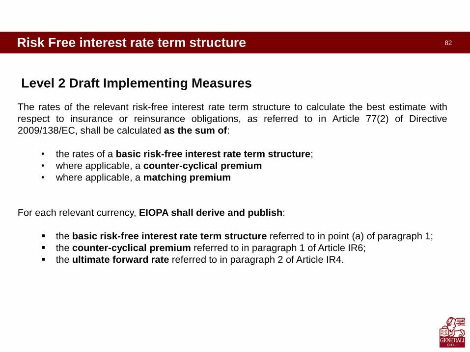
82 Risk Free interest rate term structure

Level 2 Draft Implementing Measures

The rates of the relevant risk-free interest rate term structure to calculate the best estimate with

respect to insurance or reinsurance obligations, as referred to in Article 77(2) of Directive

2009/138/EC, shall be calculated as the sum of:

• the rates of a basic risk-free interest rate term structure;

• where applicable, a counter-cyclical premium

• where applicable, a matching premium

For each relevant currency, EIOPA shall derive and publish:

the basic risk-free interest rate term structure referred to in point (a) of paragraph 1;

the counter-cyclical premium referred to in paragraph 1 of Article IR6;

the ultimate forward rate referred to in paragraph 2 of Article IR4.

83

0.00%

1.00%

2.00%

3.00%

4.00%

5.00%

6.00%

7.00%

0 20 40 60 80 100 120

Forward rates

NS50,6.1%

SW30,4.2%

MKT

The extrapolation technique (Nelson Siegel or Smith Wilson), the

extrapolation entry point and the ultimate forward rate (UFR) are key

drivers of the valuation, especially in case of long term business with

guarantees

UFR

Extrapolation technique

Entry point

Basic Risk Free interest rate term structure - extrapolation

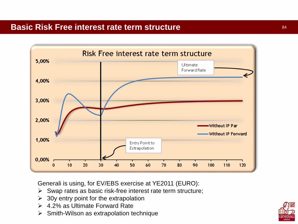
84 Basic Risk Free interest rate term structure

Generali is using, for EV/EBS exercise at YE2011 (EURO):

Swap rates as basic risk-free interest rate term structure;

30y entry point for the extrapolation

4.2% as Ultimate Forward Rate

Smith-Wilson as extrapolation technique

85 Counter – cyclical premium

Generali is supporting the Industrial proposal for CCP and, in line with last CFO Forum

statement, will disclose to Financial Markets at YE2011:

calculation using Illiquidity premium applied to forward rate

impact assessment using a govies adjustment based on Industrial Proposal

86 AGENDA








87 The MCEV calculation: a simple and “practical” example

Principles and models for the Embedded Value calculation · Principles and models for the Embedded...

Documents

Transcript of Principles and models for the Embedded Value calculation · Principles and models for the Embedded...