Principles of Principal Components -...
45
Bülent Baygün (212) 816-8001 [email protected] New York Janet Showers (212) 816-8020 [email protected] New York George Cherpelis (212) 816-8022 [email protected] New York This report can be accessed electronically via ➤ SSB Direct ➤ Yield Book ➤ E-Mail Please contact your salesperson to receive SSMB fixed-income research electronically. UNITED STATES JANUARY 31, 2000 FIXED-INCOME RESEARCH Portfolio Strategies UNITED STATES Principles of Principal Components A Fresh Look at Risk, Hedging, and Relative Value ➤ Principal Components Analysis (PCA) quantifies movements of the yield curve in terms of three main factors: level, slope, and curvature. In this context, hedging and risk management become a matter of managing exposure to these factors. ➤ Through yield curve scenarios obtained from PCA, one can set up optimal curve-neutral portfolios, implement a curve view, and perform return attribution. ➤ Butterfly trades are a popular way to identify and trade rich/cheap sectors of the curve. PCA provides a method by which to structure curve- neutral butterfly trades that isolate the relative value opportunity from any market- and slope- directional bias.
Transcript of Principles of Principal Components -...
Bülent Baygün(212) [email protected] York
Janet Showers(212) [email protected] York
George Cherpelis(212) [email protected]
New York
This report can beaccessed electronicallyvia
➤ SSB Direct➤ Yield Book➤ E-Mail
Please contact yoursalesperson to receiveSSMB fixed-incomeresearch electronically.
U N I T E D S T A T E S JANUARY 31, 2000F I X E D - I N C O M E
R E S E A R C H
Portfolio Strategies
UNITED STATES
Principles of PrincipalComponentsA Fresh Look at Risk, Hedging, and Relative Value
➤ Principal Components Analysis (PCA) quantifiesmovements of the yield curve in terms of threemain factors: level, slope, and curvature. In thiscontext, hedging and risk management become amatter of managing exposure to these factors.
➤ Through yield curve scenarios obtained from PCA,one can set up optimal curve-neutral portfolios,implement a curve view, and perform returnattribution.
➤ Butterfly trades are a popular way to identify andtrade rich/cheap sectors of the curve. PCAprovides a method by which to structure curve-neutral butterfly trades that isolate the relativevalue opportunity from any market- and slope-directional bias.

January 31, 2000 Principles of Principal Components
2
Executive Summary ............................................................................................................................... 3
Part I. Principal Components for the Entire Yield Curve 4
Principal Components Analysis for Portfolio Management — Motivation.............................................. 4
Applications of Principal Components Analysis of the Yield Curve ..................................................... 7
A Close Look at Hedging With Principal Components ......................................................................... 10
Practical Issues (or Frequently Asked Questions).................................................................................. 18
Part II — Principal Components for Structuring Butterfly Trades 23
What Makes a Good Butterfly Weighting Scheme? .............................................................................. 23
Overview of the Butterfly Model Input and Output — What to Look For ............................................ 25
Levels or Changes? A Dilemma Revisited............................................................................................. 29
Lessons From the Crisis of Fall 1998..................................................................................................... 35
Appendix A – Computation of the Principal Components..................................................................... 36
Appendix B – Methodologies for Computing Portfolio Hedges Using Principal Components ............. 37
Appendix C – What Is the “Right” Butterfly Spread to Assess Performance in a Butterfly Trade?...... 41
Acknowledgment
The authors would like to thank Victoria Averbukh, Chi Dzeng, Lauren Edwards, StewartHerman, Antti Ilmanen, Andrea Learer, Alex Li, Charlie Parkhurst, and Brian Varga for theirassistance during the preparation of this report.
Contents
January 31, 2000 Principles of Principal Components
3
OverviewSince our initial publication about Principal Components Analysis (PCA) in theAugust 1, 1997, issue of Bond Market Roundup: Strategy, we have been usingthe PCA framework extensively in our day-to-day operations for a variety ofpurposes. There has been strong interest in this approach both internally andfrom our client base. Needless to say, several interesting questions arose alongthe way, and as a result, we undertook more detailed studies that helpedimprove the understanding of PCA and also pointed the way to newapplications. In this report, we present a summary of our PCA experience.1 Ourprimary focus is on the real-world use of PCA, so a considerable portion of thereport is dedicated to practical issues. We also provide a step-by-step guide onhow to compute principal components.
There are two main parts to this report. The first part concerns PCA for yieldcurve modeling, portfolio applications, and risk management. This is the areain which our work on PCA started originally. The essence of PCA is that mostyield curve movements can be represented as a combination of three reshapingpatterns, called principal components. The most prominent applications are inportfolio risk management and hedging, especially for portfolios with cashflows along the entire yield curve. In that context, the PCs are viewed as therisk factors. Other applications covered in this section include structuringcurve-neutral trades, return attribution, and the generation of yield curvescenarios. We discuss in detail how to hedge a portfolio, using the TreasuryIndex as an example. A number of frequently asked questions are answered atthe end of Part 1. These range from whether the PCs need to be updatedperiodically to whether to use PCs from levels or changes to when the fourthPC can become important.
The emphasis in the second part of the report is in looking for relative value onthe curve, and structuring butterfly trades. As such, applications are gearedmore toward individual trades than portfolio-level decisions. We reviewdifferent weighting methods for butterfly trades, and propose a new one, basedon PCA. Our interactive butterfly model, available on the Internet throughSalomon Smith Barney Direct, is also described. Another discussion of whetherto use PCs from levels or changes appears in this part, along with extensivesimulation results that quantify the profitability of PC-based butterfly tradesusing a wide variety of model parameter values.
The Appendices contain material that is not central to our discussion but is usefulas a reference. Appendix A is a summary of the mathematics of PCs, Appendix Bdescribes the computation of portfolio hedges, and Appendix C is a discussion ofvarious ways to define butterfly spreads and their implications.
1
Some of the material in this report originally appeared in past issues of our weekly, Bond Market Roundup: Strategy.References to these articles are given at the beginning of relevant sections.
January 31, 2000 Principles of Principal Components
4
➤ The conventional approach of using duration to assess risk implicitlyassumes perfect correlation between all points on the yield curvewith no term structure of volatility. In contrast, the partial durationapproach works as if there is no correlation across the curve.Principal Components Analysis (PCA) bridges this gap by takingaccount of the correlation and volatility structure of the yield curve.
➤ PCA identifies reshaping patterns, called principal components,which explain the variance in the yield curve. Almost all of thisvariance (99.4%) is captured by the first three PCs, which represent alevel shift, slope change, and curvature change.
➤ Portfolio applications of PCA include assessing and hedging curverisk, performing return attribution, and generating realistic yieldcurve scenarios. In risk management and hedging, PCs are viewedas risk factors, and the objective is to keep the portfolio exposure toPCs within acceptable bounds.
➤ PCs calculated using large data samples give a robustrepresentation of yield curve movements in a wide variety ofenvironments. As such, PCA does not have to be updatedperiodically to adjust the PCs to the current environment. Thevolatility, but not the shape, of PCs depends on the horizon for whichthe PCs are calculated, e.g. four-week PCs are twice as volatile asone-week PCs (square-root scaling).
Principal Components Analysis for Portfolio Management —Motivation2
A number of problems in portfolio management and trading require understanding andquantifying the reshaping of the yield curve. For example, in portfolio immunization,the goal is to maintain the market value of an asset portfolio relative to a liabilityportfolio under all yield curve movements. Relative-value managers often seek toenhance returns without taking yield curve views. They seek to construct curve-neutralportfolios or trades that will outperform the market. At other times, managers wish tocreate yield curve exposure. However, to structure optimal portfolios and correctlyforecast outcomes, yield curve scenarios must be realistically modeled. Moreover,portfolio managers and traders alike need to understand the risk their positions andportfolios have to the reshaping of the yield curve.
2 Parts of this section originally appeared in the August 1, 1997, issue of Bond Market Roundup: Strategy, Salomon Smith Barney.
Part I. Principal Components for theEntire Yield Curve
January 31, 2000 Principles of Principal Components
5
For portfolio managers and traders, the first tool that comes to mind to judge marketrisk is duration — nominal or effective. Although this is largely still the tool of firstresort, investors have realized that it is an incomplete measure. While durationsmight be matched, portfolios could still be subject to performance mismatchesbecause of yield curve reshaping.3 To obtain a better understanding of portfolio yieldcurve risks, many investors have moved to partial-duration analysis, which measuressensitivity to a particular maturity point on the par curve.4 Indeed, partial durationscan add substantially to the understanding of risk gained from simple duration orduration bucketing methods. For example, a ten-year STRIP has a duration ofapproximately ten years, which is similar in duration to 20-year (roughly) bonds.However, from a yield curve exposure point of view, the STRIP can perform verydifferently from either a 20-year bond or a ten-year note.5
Although partial durations certainly enhance understanding, partial durations are, in asense, too complete. They provide too much information. This is because partialdurations define sensitivities to each point on the par curve independently. They donot take into account the correlation between points on the curve. They also do notaccount for the varying yield volatilities along the curve. For example, if a portfolio islong the two-year sector and short the three-year sector, one position may offset theother to a large degree if appropriately weighted. Therefore, requiring that not onlydurations, but partial durations match is likely too restrictive. If the same amount ofrisk to yield curve changes could be achieved with less restrictive constraints,investors will be open to a broader universe of relative-value opportunities.
To assess risk more efficiently, we need to succinctly describe the reshaping of theyield curve. One technique that can be used to analyze yield curve reshapings is astatistical approach called principal components analysis (PCA). Market participantsthink of yield curve movements in terms of three components: (1) level shift, (2) slopechange, and (3) a curvature change (hump). PCA formalizes this viewpoint. In thissection, we provide an overview of PCA and its implications for modeling movementsin the yield curve. PCA has been applied by a number of authors to study the yieldcurve.6 All of the reported studies, including ours, aim to identify and analyze themain factors driving movements in the yield curve. We also consider variousrobustness issues, some of which we believe to be addressed in some detail for thefirst time.
In PCA, the change in the yield curve over a given period is described as a weightedsum of fixed yield curve reshapings. PCA analyzes the covariance matrix of the 3 Duration measures, of course, are regularly augmented by convexity.
4 Partial duration is also known as key rate duration and can be defined as sensitivities to either points on the par or spot yield curve.
5 The ten-year STRIP has more exposure to the ten-year par rate than a ten-year note. This is offset by negative exposures to the
seven-year, five-year, three-year, etc. — all shorter par rates. Moreover, the ten-year STRIP has no partial-duration exposure to the20-year par rate, despite a similar duration to a 20-year bond.
6 The work on yield curve applications of PCA spans more than ten years, with interest in the subject gaining momentum recently.
Some related articles include:
- Robert Litterman and José Scheinkman, "Common Factors Affecting Bond Returns," The Journal of Fixed Income, June 1991, pp. 54-61.
- Eduardo Canabarro, "Where Do One-Factor Interest-Rate Models Fail?" The Journal of Fixed Income, September 1995, pp. 31-52.
- Eric Falkenstein and Jerry Hanweck, Jr., "Minimizing Basis Risk from Non-Parallel Shifts in the Yield Curve, Part II: PrincipalComponents," The Journal of Fixed Income, June 1997, pp. 85-90.
Duration provides toolittle information about
yield curve risk . . .
... while partial durationsmay provide too much
information.
Principal componentsanalysis assesses yield
curve risk moreefficiently.

January 31, 2000 Principles of Principal Components
6
yield changes of different maturity points along the yield curve to optimallydetermine these fixed reshaping patterns, called principal components (PCs).7
For our analysis, we have used the weekly yield changes at 120 constant maturitypoints (three-month to 30-year maturity range with three-month increments) on theTreasury Model par curve for the period from January 1989 through February 1998to generate the covariance matrix. This gives rise to 120 PCs. It is important to notethat the PCs are uncorrelated with each other by construction. Therefore, none of thePCs can be written in terms of the others. Each PC contributes some uniqueinformation not provided by the other PCs.
Each PC explains a portion of the total variance. The important PCs are those thatexplain the highest percentage of the total variance. Sorting the PCs in order ofdecreasing variance, the first three components explain more than 99.4% of the totalvariance. Therefore, most movements in the yield curve can be described by usingthe first three PCs only. Discarding the remaining components omits little. Figure 1shows the individual and cumulative variances of the first three PCs. Figure 2 showsthe first three PCs scaled by the standard deviations of the PCs. The first componentaccounts for 93.5% of variance; the pattern has positive coefficients at all maturitiesand consequently represents a level shift. The second accounts for 4.9% of variance;it is negative at the short end and positive at the long end, representing a change inslope. The third accounts for 1.0% and is positive at both ends and negative in themiddle: a curvature component.
Figure 1. Variance Explained by the First Three Components
Component #1 Component #2 Component #3
Standard Deviation 2.77 bp 0.63 bp 0.29 bpProportion of Variance 93.5 % 4.9 % 1.0 %Cumulative Proportion 93.5 98.4 99.4
Source: Salomon Smith Barney.
Figure 2. The First Three Principal Components for a One-Month Horizon Computed from Weekly YieldChanges, Jan 89-Feb 98
Years to Maturity
Yie
ld C
hang
e (b
p)
0 5 10 15 20 25 30
-10
010
2030
0 5 10 15 20 25 30
-10
010
2030
PC #1: LevelPC #2: SlopePC #3: Curvature
Source: Salomon Smith Barney.
We have interpreted the first component as a level shift, despite the fact that it is nota pure parallel shift. Thus, the first component includes the slope and curvature
7 The fixed patterns are called loadings and the random weights are called principal components (PCs). However, in discussion, the
terms are used more loosely with the fixed patterns also referred to as PCs, with the principal components called weights.
The first threecomponents explain ahigh percentage of allyield curve variation.
The interpretation of thecomponents is intuitive.

January 31, 2000 Principles of Principal Components
7
changes that are correlated with yield level changes. With an upward move in rates(a positive realization of the first PC), the short end of the curve (out to about fouryears) steepens and the long end flattens, increasing the hump in the intermediatesector of the curve. This observation is in agreement with two often-heardstatements: (1) bear-flatteners are more likely than bear-steepeners and (2) the hump(curvature) of the curve becomes more pronounced when yield levels rise. Similarly,for a decline in yields (a negative realization of the first PC), bull-steepeners aremore likely than bull-flatteners. These arguments are based on the first componentalone, which, due to its high variance, explains the gross behavior of yield curvemovements. However, to a lesser extent, the second and third components alsocontribute to movements in the yield curve, which explains why bear-steepeners andbull-flatteners occur, albeit less frequently.
Applications of Principal Components Analysis of theYield CurveThere are several ways in which portfolio managers and traders can benefit fromyield curve PCA. We focus on four applications: assessment of risk, hedging, returnattribution, and constructing yield curve scenarios.
The reshaping scenarios of PCA can be used to efficiently quantify the risk in aportfolio. As discussed in our introduction, duration assumes a perfect 1-for-1correlation between the changes in yields of different maturities, and is thus prone tomisquantify the risk in a portfolio by not accounting for the effects of reshaping.More specifically, since the curve tends to flatten when yields increase and steepenwhen yields decrease, a portfolio that is solely duration-matched is likely to have aresidual directional bias. In contrast, partial duration may find too much risk by notaccounting for the covariance structure. However, PCA has determined a set of threefactors (reshaping patterns, or PCs) that account for an extremely high proportion ofthe variance in the yield curve. By comparing a portfolio’s sensitivity to changes ineach of these PCs to the sensitivity of a benchmark, a good measure of the yieldcurve risk of a portfolio versus its benchmark can be obtained with only threenumbers. Moreover, the three PCs represent independent sources of yield curve risk.Therefore, one can easily obtain the total risk of the portfolio from the individual PCrisks and compare this total against allowable risk limits8.
It is interesting to note that a duration-matched portfolio need not have zerosensitivity to the first PC, the level component, because of the covariance structureof the yield curve. A 10s-30s duration-neutral flattening trade will have positiveexposure to the first PC. It will do well in a bear market because 10s-30s tend toflatten in a bear market. The second PC, the slope component, only representschanges in slope that are not correlated with level changes.
The reshaping patterns determined by PCA can be used to help structure curve-neutralportfolios. If a position has zero exposure to each of the first three PCs, then it will
8 The total risk of the portfolio is calculated as follows: first the P&L for a 1-standard-deviation move in each of the three PCs is
calculated (in the Yield Book). Under a first order approximation, the squares of those three numbers are the variances ofindependent components of the total P&L. So, the variance of the total P&L is simply the sum of these component variances. Oncethe variance has been found this way, it is straightforward to compute the value-at-risk at the 5% or 1% levels using a normaldistribution assumption.
Using PCA to assess risk.
Using PCA to structurecurve-neutral hedges.

January 31, 2000 Principles of Principal Components
8
have zero exposure to any movement in the yield curve that is a linear combination(weighted sum) of the first three PCs (this is to the first order, ignoring the convexityeffects of large rate moves). This fact is useful in structuring portfolios. By optimizingan objective function, such as the maximization of dollar return subject to constraintsthat the exposure to the three PCs is zero, the optimal curve-neutral portfolio can bedetermined. This portfolio will be more curve-neutral than one structured to simplymatch duration. The portfolio will likely have a superior value of the objectivefunction than one structured to match partial durations all along the curve because thenumber of constraints on the portfolio has been reduced to three. Once again, note thatthe resulting portfolio may not be exactly duration-neutral. We will provide moredetails about hedging in the next section.
Investors like to know the breakdown of their P&L: how much of the return camefrom movements in the yield curve (such as level changes, steepening/flattening,etc.), and how much of it came from changes in spread? Furthermore, they are alsointerested in knowing to what extent their portfolio was mishedged, i.e., did theyactually have level exposure, or perhaps a slope bias, beyond what was perceived toexist in the portfolio? PCA provides a unique perspective in quantifying that part ofthe return attributable to movements in the yield curve. One can easily break downthe realized model yield curve movement over the period in question into its firstthree PCs and a residual reshaping. This is done by fitting the yield curve movementby the three PCs. Then one can calculate the returns from the fitted PCs in thefollowing manner: first, the return under the first PC alone is calculated. Then thereturn under the combined first and second PCs is calculated and the known returnunder the first PC is subtracted from the combined return to obtain the part thatcomes from the second PC. In the next step, the procedure is repeated for all threePCs combined to obtain the return due to the third PC. Finally, the return due to theresidual yield curve movement is calculated separately. That part of the realizedreturn that is not explained by the first three PCs and the residual curve movementusing this approach is attributed to spread changes and rolling yield.
If a portfolio is hedged against a specific PC, then the return due to that PC is expectedto be small. If an investor wants to eliminate level risk by hedging the portfolioagainst the first PC (level shift), only a small portion of realized return should be fromthe first PC. A strong steepening or flattening of the curve could manifest itself in thereturn from the second PC (slope change), especially if the portfolio is mishedged tothis component. Similarly, strong fluctuations in the P&L that come from the third PCmay indicate a less-than-perfect hedge against curvature changes, unless this exposureis being maintained deliberately to implement a view. By tracking the attribution ofthe total P&L to the PCs, an investor will have a realistic assessment of whetherhis/her curve-hedging strategies are meeting their goals, and take corrective action, ifnecessary, to eliminate unwanted curve exposure.
One of our initial motivations for undertaking the study of PCA was to designrealistic yield curve scenarios for use in the Salomon Smith Barney Yield Book™.Investors frequently desire a set of scenarios that cover a range of possible futureyield curve outcomes. This set of scenarios could be used to assess performance andrisk or to optimize portfolios. We propose the use of the PCs as the basis for
Using PCA for returnattribution.
Using PCA to constructyield curve scenarios.
January 31, 2000 Principles of Principal Components
9
generating realistic scenarios that are consistent with the statistical properties ofhistorical changes in the yield curve.9
By itself, the first PC looks like a reasonable scenario, but the second and third do not.Actual yield curve changes are well described by a combination of the first three PCsand are generally dominated by the first PC because of its higher variance. Therefore,to obtain more realistic-looking scenarios, we need to combine the three PCs.
We can create a new set of three scenarios by taking linear combinations of theoriginal PCs without losing any ability to explain variation in the yield curve. Anyset of three scenarios that can be obtained from and transformed back to the firstthree PCs are equivalent from a hedging and immunization standpoint. Therefore, itis possible to have different representations of the yield curve movements that areequivalent to the first three PCs, but have the advantage of looking like scenariosthat might actually occur.
The scenarios in Figure 3 are all equally likely by construction and cover a wide rangeof movements in the yield curve consistent with historical reshapings of the curve.There are bear- and bull-steepeners, bear- and bull-flatteners, and intermediatescenarios (only the bear scenarios are shown in Figure 3; the full scenarios arenegative realizations of the bear scenarios). The scenarios shown in the figure are for aone-month horizon (see below for a discussion of longer time horizons).
Users of Salomon Smith Barney's Yield Book™ have access to scenario files basedon our PCA analysis. There are three types of scenario files. In the first type, thescenarios represent the original PCs (see Figure 2). The magnitudes of the ratechanges are appropriate to the horizon period based on historical yield volatilities.The names of these scenario files are of the form “pc+horizon.” For example, the PCscenario file for a three-month horizon is named pc3mo. In the second type, thescenarios are linear combinations of the three original PCs that represent a spectrumof possible yield curve movements (see Figure 3). These scenario files are named“cmb+horizon”. For example, the combination file for a one-year horizon is calledcmb1yr. Included in each file are both positive and negative realizations of eachscenario. Finally, the third type of scenario file contains parallel shifts of �50bp and�100bp, as well as combinations of the first two PCs that are centered about theseparallel shifts; these files are named bbsf50 and bbsf100. For example, in bbsf50, thefirst PC is scaled such that it is centered about �50bp, and the second PC is scaled toone standard deviation (positive and negative), giving rise to four combinations.
9 A common method for constructing yield curve scenarios uses regression to determine the amount that each point on the curve
moves relative to a move in a benchmark maturity (e.g., the 30-year yield). Unfortunately, this method allows only one factor ofchange in the yield curve. As used here, PCA allows a richer set of yield curves, as reshapings are determined by three factors.
Scenarios based on PCAare available n the Yield
Book.

January 31, 2000 Principles of Principal Components
10
Figure 3. Combination Scenarios for a One-Month Horizon Derived from Principal Components
Years to Maturity
Yie
ld C
hang
e (b
p)
0 5 10 15 20 25 30
010
2030
0 5 10 15 20 25 30
010
2030
Bear-steepenerBear-intermediateBear-flattener
Source: Salomon Smith Barney.
It is also possible to use PCs in the Yield Book™ to generate scenarios byspecifying yield changes at only a number of points. This is useful, for example,when creating economic outlook scenarios based on certain views about specificparts of the curve. Just to illustrate, we may want to create a six-month scenario thatdepicts the following situation: The Fed hikes the Funds rate by 50bp during thenext six months; further rate hikes are expected, so the two-year goes up by 75bp;but because long-term inflation expectations are low, the 30-year barely budgesabove the +25bp mark. We can have an opinion about those three points, but beforewe can undertake any analysis, we will also need to know how the entire yield curvereshapes under these constraints. In other words, the specified changes shouldsomehow be interpolated to fill in the unknown points. PCs provide a realistic wayof performing this interpolation: the Yield Book™ can automatically compute acombination of the three PCs that satisfy the given yield changes, and since anycombination of PCs spans the entire maturity range, we have our scenario. In fact,this is essentially how we periodically generate outlook scenarios that form the basisof our recommended yield curve strategies.
Another application of PCs is to gauge the likelihood of a given scenario. A scenariois broken down into its components (by regression against PCs) and the coefficientsof the regression are compared to the standard deviations of the PCs that areappropriate for the horizon of the scenario. For example, if the coefficients represent1, -3, and 0.5 standard deviation movements in the PCs, then that scenario is atypical bearish scenario with a strong flattening (-3-standard deviations) and a mildchange in curvature. This approach allows one to compare a set of proposedscenarios with one another and judge objectively which ones are typical and whichones represent more extreme movements of the curve. The latter could be moreappropriate for stress-testing.
A Close Look at Hedging With Principal Components10
PCA is a powerful tool for managing portfolios because it allows efficientassessment of yield curve risks. However, investors initially may have difficulty 10
Parts of this section originally appeared in the February 27, 1998 issue of Bond Market Roundup: Strategy, Salomon SmithBarney.
January 31, 2000 Principles of Principal Components
11
understanding what it means to have exposure to these components and how toeffectively use them in practice. In this section, we address the followingimplementation issues:
Representation of PCs as Trades: We represent the three principal components bythree trades. Each trade involves taking long or short positions in three securities.Investors can then translate their portfolio’s exposure to the PCs to exposures tothese three independent trades. Moreover, a portfolio’s exposure can be condensed topositions — long or short — in just these three securities.
Interpreting PC Exposures: We demonstrate that the duration-dollar-weightedyield spreads of these trades can be used to monitor portfolio performance. Thedollar exposures to each component can be scaled to represent a 1bp change in theseduration-dollar-weighted yields and spreads.
Computation: We look at several methods for computing these component trades,and for calculating a portfolio's curve exposure in terms of the three securities. Fromthis information, a portfolio manager can easily determine what trades must beexecuted to eliminate any exposure.
Error Estimates: It may be hard to believe that a portfolio such as the TreasuryIndex could be reasonably replicated with holdings in only three securities. Weobtain an indication of errors by testing our hedge over 30 scenarios. The hedgeportfolio performs well, and we conclude that using principal components computedwith data from a long time period is best.
For comparison, we also assess the performance of a partial-duration-matchedportfolio using seven securities.
Selection of the Hedge Securities: We analyze portfolio hedges constructed fromseveral sets of three securities. We also assess the effectiveness of using Treasuryfutures as the hedge vehicles. We conclude that the best hedges occur when the threesecurities are “well-spaced” along the curve.
Representing Principal Components as TradesDuration has always been the initial measure to start with when assessing the risk ofa portfolio or the risk of a portfolio versus its benchmark. At first, modified(nominal) duration11 was used and later this was extended to effective duration.12 Amismatch in duration is easy to interpret — a portfolio is either long or short themarket. Eliminating this exposure by shortening or lengthening is easy to do.
Partial durations were the next step in measuring yield curve exposure. Partialdurations (or key rate durations) separate a portfolio's total duration into sensitivitiesto yield changes at several points along the curve. Thus, partial durations recognizethat yields along the curve rarely, if ever, change by the same amount. Again,interpretation is relatively easy — a portfolio is either long or short each maturitysector along the curve. It is easy to eliminate any exposure at each partial durationmaturity — simply by selling/buying the appropriate amount of notes of the same 11
Price sensitivity to a 1bp change in the yield of the security.
12 Price sensitivity to a 1bp parallel shift of the yield curve.

January 31, 2000 Principles of Principal Components
12
maturity. Moreover, selling five-year notes to eliminate mismatch in the five-yearpartial will not change exposures at any of the other six partial durations.
PCA provides a more efficient way to quantify exposure to the yield curve becauseit considers the correlations and variances of different points along the yield curve.The analysis suggests that only three factors of variation are sufficient to capturemost variations in the yield curve. However, understanding the exposure to each PCand identifying the trades to eliminate that exposure is not so easy. For example,suppose a portfolio (versus its benchmark) has exposure to the first PC — a levelshift — such that it underperforms if rates decline. Despite the fact that the first PCis not a simple parallel shift of the curve (as it includes slope and curvature changesthat are correlated with moves in market direction), a first reaction to eliminate theexposure would be to extend duration by, say, buying five-year notes. However,such a solution would eliminate the exposure to component No. 1, but likely createnew exposures to components Nos. 2 and 3. Therefore, identifying the hedge for PCexposures is more complicated.
Remember that the three PCs were determined analytically to be independent (notcorrelated) factors of variation in the yield curve. Therefore, to represent eachcomponent, we will identify a trade that has exposure to one PC but zero exposure tothe other two PCs. That is, we identify three Independent Trades to interpret andhedge the three independent PCs. Since there are three factors of variation, threesecurities should be sufficient to define these trades. Using 2s, 10s, and 30s as ourthree hedge securities, the three independent trades we have identified are shown inFigure 4. These trades have intuitive meanings and are only slightly morecomplicated than we might have hoped.13
Figure 4. Independent Trades Representing the Three Principal Components, Expressed as a Percentageof Duration Dollars
Independent Trade One Level Independent Trade Two Slope Independent Trade Three Curvature
Two-Year -15% 100% -25%Ten-Year -45 -26 10030-Year -39 -87 -88
-100% -13% -13%
Source: Salomon Smith Barney.
1 The Independent Trade for PC No. 1, an increase in yield level, is to be shortthe market. The trade is short all three securities. The amounts are chosen sothat the trade has zero exposures to PC Nos. 2 and 3.
2 The Independent Trade for PC No. 2, an increase in the slope of the curve, isa steepening trade. The trade is to be long the short end of the curve and shortthe long end of the curve. This trade is a combination of a 2s-10s steepeningtrade and a 2s-30s steepening trade, with more duration dollars in the latter.
13
It is important to recognize that simplification of these trades — for example, into a one-security level trade, or a two-security 2s-10s slope trade — would create trades that no longer have zero exposure to the other components. Then one could no longer simplyadd up the trades to find the overall portfolio hedge.

January 31, 2000 Principles of Principal Components
13
3 The Independent Trade for PC No. 3, a decrease in curvature, is a butterflytrade. The trade is long the center (10s) and short the wings (2s and 30s).
In Figure 5, we show the size of each trade that will provide a $1 million profit(exposure) to a one-standard-deviation move (over a one-month period) in eachcomponent.14 Again, these trades each have exposure to only one PC. The tradesneed not be either cash- or duration-dollar-neutral. However, notice that they areclose to duration-dollar-neutral.
Figure 5. Independent Hedge Trades for $1 Million Exposure to a One-Month One-Standard-DeviationMove in Each Component (Market Value in $ Thousands), 27 Feb 98
Analytic Solution Yield Book Optimization Solution
Independent Trade One — Level
EDUR$ Weight Market Value EDUR$ Weight Market Value
Two-Year -$5,686 15.42% -$30,537 -$5,768 15.38% -$30,976Ten-Year -16,735 45.40 -22,033 -17,021 45.38 -22,40930-Year -14,442 39.18 -10,600 -14,715 39.24 -10,800
-$36,863 100.00% -$37,503 100.00%Independent Trade Two — Slope
EDUR$ Weight EDUR$ Weight
Two-Year $57,281 100.00% $307,633 $57,051 100.00% $306,395Ten-Year -14,480 -25.28 -19,064 -15,010 -26.31 -19,76230-Year -49,055 -85.64 -36,004 -49,584 -86.91 -36,392
-6,254 -10.92% -$7,543 -13.22%Independent Trade Three — Curvature
EDUR$ Weight Market Value EDUR$ Weight Market Value
Two-Year -$71,838 -25.14% -$385,813 -$71,854 -25.25% -$385,899Ten-Year 285,769 100.00 376,235 284,535 100.00 374,61130-Year -248,715 -87.03 -182,544 -249,858 -87.81 -183,383
-34,784 -12.17% -$37,177 -13.07%
Source: Salomon Smith Barney.
Computing Portfolio HedgesWe provide a brief overview of some procedures for computing these independenttrades and replicating portfolios (or hedges) once a set of three hedge securities hasbeen selected. We defer the details to the Appendix.
We rely on the scenario analysis and optimization features of the Yield Book™ forat least part of our calculations. As we pointed out before, we have providedscenario files in the Yield Book™ that represent positive and negative realizationsof the three PCs. There are scenario files for different horizons as the componentsare scaled to the standard deviation of curve changes appropriate for the length ofthe horizon (one-, three-, and six-month). Moreover, we have created sets of yieldcurve scenarios by combining the PCs. These are the combination scenarios (or thecombos). The scenarios represent equally likely outcomes and provide a spectrum of
14
All dollar returns referred to herein are calculated using a zero-day horizon.
January 31, 2000 Principles of Principal Components
14
different types of yield curve movements. These scenarios are also available on theYield Book™ scaled for different horizons.
We suggest two methods for computing the Independent Trades that represent thethree PCs. The first is an analytic solution. If the sensitivity of each hedge securityto each component is known, it is straightforward to solve for the weights for eachindependent trade analytically by linear algebra. The second method uses theoptimization feature of the Yield Book™ to easily obtain the weights for eachindependent trade. Both procedures arrived at nearly identical solutions to theexamples we have tried.
For computing replicating portfolios (or hedges), we considered four methods: (1)calculate the hedge from the Independent Trades; (2) utilize a direct analyticsolution using linear algebra; (3) optimize in the Yield Book™ by “maxmin” on thereturn differences over the PC scenarios; and (4) optimize in the Yield Book™ by“maxmin” on the return differences over the combo scenarios. We tried all methodsfor determining the replicating portfolio of three securities for the Treasury Index.We found that all four methods produced similar results. For ease ofimplementation, we currently recommend using the method of optimization over thePC scenarios.
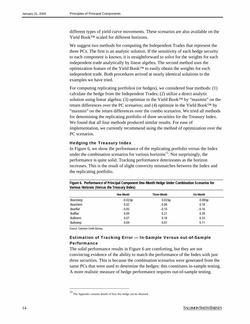
Hedging the Treasury IndexIn Figure 6, we show the performance of the replicating portfolio versus the Indexunder the combination scenarios for various horizons15. Not surprisingly, theperformance is quite solid. Tracking performance deteriorates as the horizonincreases. This is the result of slight convexity mismatches between the Index andthe replicating portfolio.
Figure 6. Performance of Principal Component One-Month Hedge Under Combination Scenarios forVarious Horizons (Versus the Treasury Index)
One-Month Three-Month Six-Month
Bearsteep -0.02bp 0.02bp 0.08bpBearintrm 0.02 0.08 0.18Bearflat -0.05 -0.10 -0.16Bullflat 0.09 0.21 0.39Bullintrm 0.07 0.18 0.33Bullsteep 0.04 0.07 0.11
Source: Salomon Smith Barney.
Estimation of Tracking Error — In-Sample Versus out-of-SamplePerformanceThe solid performance results in Figure 6 are comforting, but they are notconvincing evidence of the ability to match the performance of the Index with justthree securities. This is because the combination scenarios were generated from thesame PCs that were used to determine the hedges: this constitutes in-sample testing.A more realistic measure of hedge performance requires out-of-sample testing.
15
The Appendix contains details of how this hedge can be obtained.
January 31, 2000 Principles of Principal Components
15
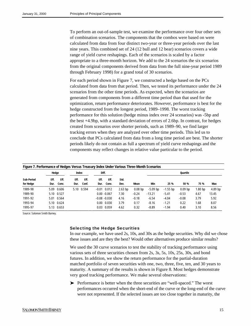
To perform an out-of-sample test, we examine the performance over four other setsof combination scenarios. The components that the combos were based on werecalculated from data from four distinct two-year or three-year periods over the lastnine years. This combined set of 24 (12 bull and 12 bear) scenarios covers a widerange of yield curve reshapings. Each of the scenarios is scaled by a factorappropriate to a three-month horizon. We add to the 24 scenarios the six scenariosfrom the original components derived from data from the full nine-year period 1989through February 1998) for a grand total of 30 scenarios.
For each period shown in Figure 7, we constructed a hedge based on the PCscalculated from data from that period. Then, we tested its performance under the 24scenarios from the other time periods. As expected, when the scenarios aregenerated from components from a different time period than that used for theoptimization, return performance deteriorates. However, performance is best for thehedge constructed from the longest period, 1989–1998. The worst trackingperformance for this solution (hedge minus index over 24 scenarios) was -5bp andthe best +4.9bp, with a standard deviation of errors of 2.6bp. In contrast, for hedgescreated from scenarios over shorter periods, such as 1989–90, we find largertracking errors when they are analyzed over other time periods. This led us toconclude that PCs calculated from data from a long time period are best. The shorterperiods likely do not contain as full a spectrum of yield curve reshapings and thecomponents may reflect changes in relative value particular to the period.
Figure 7. Performance of Hedges Versus Treasury Index Under Various Three-Month Scenarios
Hedge Index Diff. Quartile
Sub-Period Eff. Eff. Eff. Eff. Eff. Eff. Std.for Hedge Dur. Conv. Dur. Conf. Dur. Conv. Dev. Mean Min 25 % 50 % 75 % Max
1989-98 5.09 0.606 5.10 0.594 -0.01 0.012 2.63 bp 0.08 bp -5.09 bp -1.55 bp 0.09 bp 1.80 bp 4.89 bp1989-90 5.10 0.527 0.00 -0.067 7.30 -0.24 -13.21 -5.41 -0.53 4.67 13.451991-92 5.01 0.564 -0.08 -0.030 4.16 -0.18 -6.54 -4.04 -0.08 3.79 5.921993-94 5.10 0.624 0.00 0.030 3.79 0.17 -8.16 -1.21 0.22 1.68 8.071995-97 5.13 0.653 0.03 0.059 4.62 0.32 -8.89 -1.94 0.40 3.10 8.56
Source: Salomon Smith Barney.
Selecting the Hedge SecuritiesIn our example, we have used 2s, 10s, and 30s as the hedge securities. Why did we chosethese issues and are they the best? Would other alternatives produce similar results?
We used the 30 curve scenarios to test the stability of tracking performance usingvarious sets of three securities chosen from 2s, 3s, 5s, 10s, 25s, 30s, and bondfutures. In addition, we show the return performance for the partial-durationmatched portfolio of seven securities with one, two, three, five, ten, and 30 years tomaturity. A summary of the results is shown in Figure 8. Most hedges demonstratevery good tracking performance. We make several observations:
➤ Performance is better when the three securities are “well-spaced.” The worstperformances occurred when the short-end of the curve or the long-end of the curvewere not represented. If the selected issues are too close together in maturity, the

January 31, 2000 Principles of Principal Components
16
correlation between their performance will be high. Then the issues will not ascompletely represent the distinct sources of variation in the yield curve.16
➤ Replacing 30s with 25s improved the tracking error. It also reduced theconvexity of the hedge position. Likely, 25s hedge the bond sector better thancombinations of 5s/10s and 30s on average.
➤ The partial-duration-matched portfolio of seven securities did not providesuperior performance to the three security hedges under these scenarios. Onepossible reason is that the methodology for computing partial durations assumesstraight-line interpolation of the yield curve between the partial maturities. Asecond reason may be the use of 30s instead of 25s.
➤ The hedges with futures performed comparably to hedges with cash securities.However, these hedges do not provide the smallest tracking errors. Possiblereasons include the fact that bond futures represent 17-year bonds, leaving 13years of the curve beyond the hedge instrument. In addition, ten-year and five-year futures actually represent a separation of only 2.5 years along the curve.
Figure 8. Selection of Hedge Vehicles — Performance of Hedges Versus the Treasury Index Under Various Three-Month ScenariosHedge Index Diff Quartile
Eff. Eff. Eff. Eff. Eff. Eff. Std.Dur. Conv. Dur. Conv. Dur. Conv. Dev. Mean Min. 25 % 50 % 75 % Max
2s, 5s, 25s 5.10 0.644 5.10 0.594 0.00 0.050 1.29 bp 0.26 bp -2.51 bp -0.15 bp 0.30 bp 0.70 bp 3.01 bp3s, 10s, 25s 5.07 0.606 -0.03 0.012 1.54 0.07 -2.70 -1.16 0.04 1.23 3.10PDUR$ Hedge 5.10 0.597 0.00 0.003 1.58 -0.01 -3.10 -1.08 0.00 1.15 3.102s, 5s, 30s 5.12 0.710 0.02 0.116 1.65 0.58 -3.04 -0.16 0.52 1.91 3.362s, 10s, 25s 5.08 0.572 -0.01 -0.022 1.97 -0.09 -4.50 -1.74 -0.05 1.51 4.082s, 10s, 30s 5.09 0.606 -0.01 0.012 2.33 0.08 -4.97 -1.34 0.07 1.51 4.762s, 10s, 30s Futures 5.08 0.409 -0.02 -0.185 2.51 0.36 -6.31 -0.56 0.49 1.67 6.465s, 10s, 30s Futures 5.07 0.623 -0.03 0.029 2.71 -0.95 -6.75 -2.75 -1.00 0.49 4.215s, 10s, 30s 5.13 0.755 0.04 0.161 2.80 0.81 -5.25 -0.52 0.79 2.12 6.842s, 5s, 10s 5.07 0.444 -0.03 -0.150 6.68 -1.20 -18.40 -6.09 -0.64 3.51 10.48
Source: Salomon Smith Barney.
Monitoring Performance with PCsThere is one complaint that we frequently hear about principal components. Whendeveloping the Independent Hedges and replicating portfolios above, we did so bymeasuring the dollar exposure to a one-standard-deviation move in each of thecomponents. Unfortunately, investors and traders do not relate easily to thisexposure. Is a $1,000 sensitivity large or small? When the curve changes, how canone use these exposures to estimate performance?
In contrast, duration and partial durations are easier for investors to interpret. Withduration, a duration-dollar mismatch of $1,000 implies a return gain of $1,000 ifyields decline by 1bp. And a five-year partial duration-dollar mismatch of $1,000implies a return gain of $1,000 if five-year yields decline by 1bp (and yields at theother six partial duration maturities remain unchanged).
16
We have also observed that if one allows too many (for example, all Treasuries) in the optimization universe, one risks obtainingnon-intuitive solutions. Moreover, sometimes with a large optimization universe, highly leveraged solutions may result when ahedge solution includes both long and short positions.

January 31, 2000 Principles of Principal Components
17
The Independent Trades give us the means by which to provide similarinterpretations of PC exposures. The change in yield of each of the hedge securitiesfor a one-month one-standard-deviation move of each PC is shown in Figure 9. Foreach component, the magnitude of the one-standard deviation move can be capturedby a single number — the change in the duration-dollar-weighted (DD-weighted)yield/spread of the Independent Trade, where the DD-weighted yield is calculatedusing the DD weights in Figure 4. Thus, a one-standard deviation move in PC No. 1represents a 27bp increase in yields, in PC No.2 is a 17bp steepening of the curve(mainly between 2s and 30s), and in PC No.3 is a 3.5bp narrowing of the weighted2s-10s-30s butterfly spread.
Therefore, the Treasury Index has a -$30 million exposure to a 27bp increase in theduration-dollar-weighted yield of securities in Trade No. 1, or a -$1.11 millionexposure to a 1bp increase. Similarly, The Treasury Index has a $69,400 exposure toa 1bp widening of the duration dollar weighted yield spread of the 2s versus 10s and30s slope trade. Moreover, the Index has a -$3,429 exposure to a 1bp narrowing ofthe 2s-10s-30s duration dollar weighted butterfly spread. By following these threeduration-dollar-weighted yield/spreads — which represent the 3 PCs — investorsshould be able to estimate and understand their portfolios’ performance.
Figure 9. Scenario Yield Changes for the Hedging Securities
Level Slope Curvature
Two-Year 28.40 bp -13.40 bp 1.00 bpTen-Year 28.70 0.50 -1.8030-Year 24.80 4.60 1.70
Source: Salomon Smith Barney.
Summary of Hedging ResultsOur results are encouraging. We have shown that the three principal components canbe interpreted intuitively in terms of three independent trades. Trades involvingthese issues can capture the major sources of variation in the yield curve. Moreover,the Treasury Index can be well represented by a portfolio of only three issues, andyet the tracking errors appear to be reasonable. We end this section by raisingseveral issues.
➤ The Treasury Index has virtually no optionality. Thus, our hedges providereasonable matches to the convexity of our Index. Convexity obviously will bemore of an issue with mortgage and corporate portfolios.
➤ The selection of the three issues to use for hedging/replication should depend onthe application. For example, for the one- to five-year Treasury Index, 2s, 3s,and 5s will likely provide better hedges than 2s, 10s, and 30s. The general ruleof thumb is to adequately distribute the three issues along the relevant portion ofthe yield curve.
➤ Individual security hedges likely will contain more tracking error than will theindex as a whole, which is confirmed by initial work on hedging a long zero.
January 31, 2000 Principles of Principal Components
18
➤ While 2s/5s/25s provided less tracking error versus the Treasury Index than2s/10s/25s, the latter may be more appropriate when a portfolio includes sizableweighting in STRIPS in the ten- to 20-year sector of the yield curve.
Practical Issues (or Frequently Asked Questions)When using PCA for portfolio applications, a number of issues arise as to howstable the components are or how applicable the results are to different situations.We consider some of these questions below.
The PCs are derived from the covariance matrix of the weekly yield changes from1989 to 1998. An important issue to explore is whether the same results would beobtained using data from a portion of that period. We found that data from differentperiods gave rise to qualitatively the same type of components: the first always playsthe role of a level shift, while the second and the third play the role of a slope andcurvature change, respectively. The first three PCs explained more than 99% of thevariance, regardless of the data period.
However, there are some differences in the precise characterization of individualPCs. For instance, during the 1997–1998 period, the PCs of both the first and thesecond components have a much flatter shape than that in most previous periods.This suggests that, over this period, the curve has shifted more in a parallel fashion.Furthermore, the hump in the first component seems to have moved from about thethree-year point out to longer maturities (about the seven-year point for 1997–1998).None of this is surprising, given the relative stability of the Fed and the yield curveover this period.
Nevertheless, when taken as a whole, the first three components are able toconsistently explain the variation in the yield curve. We found that the first threePCs from any given sub-period can be replicated very closely by some linearcombination of the PCs from the entire 1989–1998 period. Therefore, our first threePCs, when used together, form a very good proxy for movements in the yield curveover any sub-period from 1989 through today. The difference is in the magnitude ofthe variance of each PC. The hedging results we highlighted in the previous sectionreinforce our belief that the long-term PCs should be preferred in general, becausethey subsume the largest variety of monetary policies and economic conditions. PCsfrom a shorter time period may work better during that period (in-sample), but arelikely to be inferior over the long run (out-of-sample).
Each PC remains fairly stable, regardless of the length of the interval over whichyield changes are computed. However, the length of the interval affects the varianceof the PCs. Not surprisingly, a comparison of weekly and monthly changes showsthat the variance is proportional to the length of the period. For example, the weeklychange PCs have one-fourth the variance of the monthly change PCs; the three-month yield change PCs have three times the variance of the monthly change PCs,and so on.
The PCA results discussed thus far were based on movements in the par curve.Applying PCA to spot curves produces similar qualitative interpretations. Namely, thefirst three components represent level, slope, and curvature. Transforming the spotcurve PCs to the par space, we found that the par curve movements implied by the
Do the PCA factors varyover time?
Do the PCs depend onthe data frequency?
Are the PCs based onpar and spot curves
consistent?

January 31, 2000 Principles of Principal Components
19
spot curve PCs are essentially the same as the original par curve PCs. Consequently, itdoes not matter which set of PCs we use to model the yield curve movements.
A portfolio constraint that a portfolio match the duration of a benchmark is the sameas requiring immunization to a parallel shift of the curve. To study the effectivenessof this constraint, we repeated the PCA forcing the first PC to be a parallel shift.17
As before, the second and third components represent slope and curvaturecomponents. Figure 10 shows the comparison of the variances explained by the twosets of PCs. The first three components in both sets of PCs explain the samepercentage of the total variance. However, the parallel shift explains less of the totalvariance than the original first component because the magnitude of the hump is notpresent in the parallel shift. However, the lack of hump in the parallel shift is madeup for by a more pronounced hump in the third PC than its counterpart in theoriginal set of PCs. Any shape that can be produced by the parallel shift PCs can bereplicated effectively by the original PCs, and vice versa. This indicates that if wehedge against a parallel shift (i.e., match durations) and the slope and curvaturecomponents, we will do just as well as we would if we hedged against the optimalPCs. Conversely, a hedge constructed using the original three PCs tends to producea duration-neutral portfolio.18
Figure 10. Variance Explained by the Original and Parallel Shift PCs
Cumulative Proportion of Variance
Component No.1 Component No. 2 Component No. 3
Original PCs 93.5 % 98.4 % 99.4 %Parallel Shift PCs 92.3 97.3 99.4
Source: Salomon Smith Barney.
This is a hotly debated issue. As a general rule, we believe that yield change PCs aremore suitable for hedging and risk management purposes. This is typically the waywe have been using PCA on the yield curve. In hedging and risk management, theemphasis is on minimizing the adverse effects of short-term movements in the yieldcurve. This is achieved by the constant rebalancing of one’s portfolio. As a result,longer-term mean-reversion — which would involve yield levels — of the yieldcurve is less relevant for day-to-day management of portfolio risk.
Before we get into the discussion, let us first give a caveat: PCA does not recognizethe time series aspect of its input data, be it yield levels or changes. In other words,given the data (for example, the weekly changes), we could scramble their order intime, do PCA on the scrambled data set, and would still obtain the same PCs. Theimplicit assumption in PCA is that the data are independent and identicallydistributed. This assumption would be violated, for example, if we were doing PCAon yield changes, and the changes depended on the yield levels. Of course, what wejust described, i.e., changes depending on levels, is the gist of mean-reverting term-structure models, which have intuitive appeal. In contrast, the assumption of
17
Actually, we applied PCA after first removing the parallel shift component from the weekly yield changes.
18 This is because the parallel shift is closely approximated by a linear combination of the original three components.
What happens if the firstcomponent is forced to
be a parallel shift?
Should we use PCscomputed from yield
levels or yield changes?

January 31, 2000 Principles of Principal Components
20
independent and identically distributed changes is consistent with a random walkmodel, and, in particular, could give rise to negative yields. Therefore, strictlyspeaking, simple-minded PCA on yield changes cannot be consistent with a mean-reverting framework, in which changes would exhibit positive correlation (i.e., atrend) if levels were either at too high or too a low value in their ranges. However,this trending behavior in changes may not be statistically significant in theintermediate range of level values, especially when the yield curve is close to its“typical” shape. Because levels are more likely to take values around this typicalshape than around extreme curve shapes, change data will likely be dominated bysamples with little or no observable serial correlation. This reasoning provides somecomfort about the assumption of independence in the change data.
Another issue is how long a time period to use to calculate the PCs. In general, it isbetter to use a very long time period. That way, periods of different monetarypolicies and economic environments are included, and any period-specificidiosyncrasies of the data have less of an influence on the calculated PCs (or, at leastany quirky behavior is balanced by something opposite that is present in otherperiods of the data). As a result, analysis of long-term data should indeed give rise toreliable PC estimates. This is true for both level and change PCs.
The foregoing discussion highlights the shortcomings of PCA based solely onchanges or levels. Either approach would leave some questions unanswered. Itseems that a more promising solution could be found by somehow combining thetwo extremes. That solution, we believe, probably starts with modeling the yieldcurve as a stochastic process, very much in the spirit of term-structure models. Onthe other hand, we should reiterate that, with judicious use, rudimentary PCA hasproven to be a very powerful tool for portfolio management (especially inTreasuries).
Despite the fact that the first three PCs explain more than 99% of the variance in theyield curve movements in the long run, there may be periods when the higher orderPCs may have more explanatory power than the implied sub-1% level. However, fromour experience, such episodes are rather rare and short-lived. So, hedging should notbe based on the higher order PCs in general, and definitely not at the expense of ahedge against the first three PCs. Moreover, the fourth PC (or any of the higher-orderPCs) is not as stable as the first three PCs. In other words, the reshaping implied by thefourth PC (not just the volatility of it) changes drastically depending on the timeperiod used (see our discussion on the stability of PCs above). Any hedge based onsuch a fickle statistic will not be reliable. That said, a portfolio that is perfectly hedgedagainst the first three PCs will have its primary curve exposure because of the fourthPC. But again, since the variance of that PC is very low, the residual P&L volatilitydue to this exposure will likely be small. For reference, Figure 11 shows the fourthPC. It implies a richening of the five- to 15-year sector of the curve relative to the two-year sector and the long end. An interesting interpretation of the exposure to the fourthPC is provided by viewing the exposure as relative value in a portfolio. For example,if recent movements in the yield curve observed in the market imply an extremerealization for the fourth PC (several standard deviations), then one could expect areversion of this behavior, such that the long-term standard deviation and the zero-mean property are maintained. This means that there is a possible relative-value
Does the fourth PC everbecome important?

January 31, 2000 Principles of Principal Components
21
opportunity in the market. From that perspective, an exposure to the fourth PC couldbe a measure of the possible P&L if
a reversion (an opposite realization of that PC) does indeed occur, assuming that thefirst three PCs are hedged.
Figure 11. The Fourth Principal Component for a One-Month Horizon Computed from Weekly YieldChanges, Jan 89-Feb 98
Years to Maturity
Yie
ld C
hang
e (b
p)
0 5 10 15 20 25 30
-10
-8-6
-4-2
02
Source: Salomon Smith Barney.
The PCs we have described so far are designed to model the movements of the entireyield curve. For those investors whose assets and/or liabilities are concentrated inthe short end, PCs that are custom-made for that end may be a more accurate model.Figure 12 shows the PCs for the 0- to five-year and 0- to ten-year maturity ranges.Despite the differences in their values and where they intersect the 0bp line, thesePCs possess certain common characteristics with their full-maturity-range brethren:the first PC is still a level shift with no zero-crossing, the second a slope change, andthe third, a curvature change. The first three PCs explain 99.5% and 99.4% of thevariance in the 0- to five-year and 0- to ten-year range, respectively. What isinteresting is that one can closely replicate either set of short-end PCs by somecombination of the 0- to 30-year PCs. However, the weights used in thesecombinations represent several standard deviation movements for the 0- to 30-yearPCs, which are not very likely. Turning this argument around, a one-standard-deviation move in the 0- to 30-year PCs could give rise to larger movements in theshort end than warranted by an analysis of that sector alone. As a result, theexposures for a short end portfolio obtained from the 0- to 30-year
Are the yield curve PCssuitable for investorswith exposure to the
front end of the curveonly?

January 31, 2000 Principles of Principal Components
22
Figure 12. The First Three Principal Components for a One-Month Horizon Computed from Weekly YieldChanges in the 0- to Five-Year and 0- to Ten-Year Sectors, Jan 89-Feb 98
PCs for the 0-5Yr Sector
Years to Maturity
Yie
ld L
evel
(%
)
1 2 3 4 5
-10
010
2030
LevelSlopeCurvature
PCs for the 0-10Yr Sector
Years to Maturity
Yie
ld L
evel
(%
)
0 2 4 6 8 10
-10
010
2030
LevelSlopeCurvature
Source: Salomon Smith Barney.
PCs may not adequately represent the risks in the portfolio. Our conclusion is that ashort-end portfolio is better managed with the short-end PCs.

January 31, 2000 Principles of Principal Components
23
➤ Butterfly trades allow one to identify and trade rich/cheap sectors ofthe curve. PCA provides a method by which to structure curve-neutral butterfly trades that isolate the relative-value opportunityfrom any market- and slope-directional bias.
➤ The Salomon Smith Barney Butterfly Model, available through SSBDirect, provides a powerful platform from which to look for relativevalue using butterfly trades. One can quickly analyze trading signalsand hedging properties from many perspectives using differentweighting methods and several types of data, such as Treasurymodel data, futures CTDs, coupon Treasuries, and STRIPS.
➤ After extensive historical simulations, we conclude that (i) theButterfly Model using PCA on yield levels as the weighting method ispreferable to PCA on yield changes; and (ii) the analysis should bebased on a long-enough (three or four years) window of data.
We are frequently asked about butterfly trades or specific sectors of the curve. Toprovide a framework for answering these questions, we have developed a novelButterfly Model. This model is available through an interactive screen on ourSalomon Smith Barney Direct Internet site, under US Governments/ResearchModels. The model, which can be applied to any three-legged trade, offers a newanalytical approach to evaluating butterflies. The new application can be used to:
➤ Evaluate which sectors of the curve — coupon Treasuries or STRIPS — are richand cheap.
➤ Analyze the market and slope directionality of any butterfly weighting.
➤ Identify the appropriate weights for a butterfly trade under a variety of methods.
The Butterfly Model is easy to use and incorporates several operations into one,producing a concise summary of a particular butterfly trade. We are making ourconstant maturity Treasury model and STRIPS curves available for use in thebutterfly model.
What Makes a Good Butterfly Weighting Scheme?Investors undertake butterfly trades for two main reasons: (1) to take on marketdirection or slope exposure within a cash and/or duration constraint, or (2) toundertake a curvature or relative-value trade.
1 In the first case, the duration-dollar (DD) neutral investor, for example, wouldsell bullets to buy barbells when expecting the curve to flatten, and would buybullets when expecting the economy to slow and the Fed to ease.
Part II — Principal Components forStructuring Butterfly Trades
Some investors dobutterflies to take on
market exposure, somedesire a market-neutral
relative- value trade.They will use different
weightings.

January 31, 2000 Principles of Principal Components
24
2 In the second scenario, the relative-value investor desires to take advantage of therelative cheapness or richness of one security (center) compared to two securities(wings) around it, without taking a market directional view. The expectation isthat the center security will come back in line with the wings. This investor willwant to make the assessment of value independent of changes in market directionor curve slope, and will want to know how to weight the trade to eliminatemarket or slope biases.
The two most common butterfly weightings are: (1) a 50-50 weighting (putting 50%of the duration-dollars in the short wing and 50% in the long wing), and (2) a cash-neutral and duration-neutral weighting. While these weightings match the duration-dollars of the buy-side and the sell-side, they ignore the fact that the three yieldsmay have different volatilities and imperfect correlations. Therefore, these commonweighting schemes typically produce residual market-level and slope exposure. OurButterfly Model can be used to evaluate the magnitude of these exposures.
In order to structure market-neutral butterflies for pure relative-value plays,investors look toward statistical methods, such as regression analysis19 or volatilityweighting.20 These techniques get us part of the way there, but can have someshortcomings. To construct a butterfly-weighting scheme that produces a puremarket-neutral curvature play, we recommend using principal components analysis(PCA) on the yields of the three legs of the trade. Principal component analysis21 is ageneral statistical method used to analyze the variation in multivariate series. Usingboth the historical volatility and correlation structure among the three yields, PCAwill identify the weightings to best immunize a butterfly trade to both market-leveland slope factors22 — the first two principal components — while leaving theexposure to curvature (or relative value), which is the residual variation among thethree yields. Furthermore, because of a fundamental property of PCA, the PCA-weighted butterfly spread is not correlated with market level and slope (the first andsecond components). This characteristic is the key to constructing curve-neutralbutterfly trades.
Because PCA is not based on the premise of a parallel shift, the duration-dollarweights of the wings can, and typically do, add up to something other than 100%.23
With a traditional duration-dollar matched butterfly trade, buying the center istypically a trade that is long the market in reality. By selling a little bit more than100% of the duration-dollars on the buy-side, the market directionality is removed,
19
In this application, for example, ordinary regression analysis suffers from the ambiguity involved in specifying the independentand dependent variables. That is, the betas depend on what is regressed against what. For example, X regressed on Y and Y regressedon X may result in two betas that are not the inverse of each other (the ratio of the two betas is the ratio of the variances of X and Y).This discrepancy, in turn, gives rise to different duration-dollar weights, depending on how the regressions are run.
20Volatility weighting recognizes the term structure of volatility across the curve, but assumes perfect correlation between points on
the curve. In effect, it is a one-factor approach to modeling the curve.
21See also our writings on PCA for the entire yield curve, which appeared in the August 1, 1997, issue of Bond Market Roundup:
Strategy.
22No a priori definition of market level or slope is required. The technique finds the best way to hedge systematic variation among
the three yields. The PCA weighting produces the butterfly spread with minimum variation. The residual variation can be thought ofas the relative value or curvature play.
23Similarly, the weightings do not necessarily produce cash-neutral trades.
Duration-dollar-neutralbutterflies have marketexposure. Our Butterfly
Model assesses “howmuch.”
PCA has advantagesover common statistical
methods for weightingmarket-neutral
butterflies.
PCA weights aregenerally not duration-dollar-neutral, but they
are market-neutral.

January 31, 2000 Principles of Principal Components
25
but at the expense of the duration-dollar match. We believe that because PCAprovides a more realistic yield curve model than a parallel-shift model, investorsshould not necessarily insist on matching duration-dollars.24
Whether or not the PCA weights are used in executing a trade, we believe that theyare a useful framework for evaluating the relative value of a sector. In summary:
½ As many traditional butterfly spreads are market-directional, the PCA analysisallows one to evaluate when a sector of the curve has cheapened or richenedbeyond that prescribed by recent yield movements. If a sector looks cheap basedon PCA weights (versus the wings) and a traditional butterfly has a bullish bias,the butterfly trade is likely to be a good way to go long the market (with anadded relative-value kicker).
½ The PCA analysis is a good way of identifying rich and cheap sectors of theyield curve, in which the relative valuation is independent of market direction.Portfolios of the cheap sectors can then be structured into curve-neutralportfolios, or into portfolios that have desired market exposures.
Overview of the Butterfly Model Input and Output —What to Look ForWe offer the user a variety of historical yield series to use in the analysis. Becauseissues roll down the curve, over time shortening their durations and maturities, weprefer to analyze constant maturity yield series. We have made our constant maturity(CMT) Treasury Model curve and CMT STRIPS yield series available. However,users can also choose to analyze the yield series of specific notes, bonds, andSTRIPS, if so desired25 (see Figure 13). In our example, we use CMT TreasuryModel par curve data to analyze a 4s-10s-27s butterfly, in which we buy 10s. Ourweighting method for the example will be PCA applied to the yields of the threepoints on the CMT par curve.
24
However, keeping in mind those investors who might be constrained to be duration-dollar matched, in the butterfly model we alsoprovide an option to run PCA with a slight modification to get weights that ensure duration-dollar matching.
25Other alternatives include the yield series of rolling benchmarks, rolling old benchmarks, and the issues that are currently the
cheapest-to-deliver into the Treasury futures contracts.
Use the PCA frameworkto identify cheap sectors,
even if executing withother weights.
We recommend usingthe CMT Treasury Model
or CMT STRIPS yields forthe analysis.

January 31, 2000 Principles of Principal Components
26
Figure 13. Various Data Models Available on the Butterfly Model Input Screen
Source: Salomon Smith Barney.
The main output of the Butterfly Model is a page of eight graphs for assessing therelative value and historical performance of the trade (see Figure 14). Therecommended duration-dollar weighting for the trade is also reported on the page ofgraphs. The first, third, and fourth rows have pairs of graphs: the left, a scatter plot,and the right, the time series of the residuals (distance from point to the fitted line)of the scatter plot. The current value of the residual, beta, correlation, and thepercentile of the residual over the history are reported below the graphs. The secondrow shows the time series of the butterfly spread26 obtained using the calculatedweights, as well as the time series of market level and slope. While there is muchinformation on this page of eight graphs, we suggest focusing on the following:
1 “Quick” Relative Value: The first row gives a quick read on relative value byscattering the spread of the long wing27 versus the spread of the short wing. Thisis equivalent to looking for value in a 50-50 weighted butterfly trade. Althoughnot perfect, this is commonly used by market participants. If the current point isabove the fitted line, as in Figure 13, it suggests that the middle of the butterfly ischeap.
2 Recommended Weights: The recommended DD-weights for the trade,calculated according to the method specified by the user, are listed below the left
26
Our definition of butterfly spread differs from market convention and is more directly related to the P&L potential in the trade;see the Appendix for a detailed discussion of this issue.
27Because we are long the center in this example, the long wing spread is defined as 10s minus 27s, and the short wing spread as 10s
minus 4s, so that a point below the fit line indicates richness of the buy-side security.
The main output is apage of eight graphs.
Focus on the followingitems:

January 31, 2000 Principles of Principal Components
27
graph in row 2. The graph shows the duration-dollar weighted yield spread28 ofthe butterfly. In our example, 36 duration dollars in 4s and 67 duration dollars in27s would be sold for every 100 duration dollars of 10s bought.
3 Correlation with Market Level: The left graph in Row 3 evaluates thecorrelation of the trade with market level. A near-zero correlation results in ahorizontal fit line through the points. Look for a very high (or low) residualpercentile (printed below the right graph), which indicates a good time to buy (orsell) the center.29 The value of the current residual is the deviation of the currentspread (in bp) from the average and, therefore, is an indication of the expectedreturn potential from the trade.
4 Correlation with Slope: The graphs in Row 4 evaluate the correlation of thetrade with curve slope. Again look for very high or very low percentiles.
5 Mean Reversion: It is important to evaluate the pattern of the butterfly spreadand the residuals for mean reversion. We prefer butterflies with spreads (orresiduals) that periodically cycle in a band — i.e., high values should follow lowvalues, and vice versa, in a somewhat cyclical fashion. If the spreads (orresiduals) are not cycling but trending, we would suggest further analysis of thetrade and the factors potentially driving the relative value. Perhaps a longerhistorical time frame would be appropriate.
If requested, a trade report (see Figure 15) can be generated that details theexecution of the trade with specific securities. The report includes the par, marketvalue, and duration-dollar weights for the trade. The report will include cash ifneeded to match market values.
28
In our example, the DD-weighted yield spread = (yield of center) - 36% * (yield of short wing) - 67% * (yield of long wing). Thisdefinition is different from the traditional butterfly spread — defined as twice the yield of the center minus the sum of the yields ofthe wings. Note that, even in the case of a 50-50 weighted butterfly trade, the DD-weighted spread will be one half the traditionalbutterfly spread.
29We prefer this percentile to that in (1) above as an indication of relative value, as it removes market-directional biases.
The model also producesa trade report with
details.

January 31, 2000 Principles of Principal Components
28
Figure 14. The Results of the Butterfly Model Run for 4s-10s-27s Trade
•
•••
••
•••
•• •• ••
••••
•••• ••
••••
•••• • •
••
• •
•
••
•• • •
• ••
••
•••
••••• •••
• •••• •
••
•
•••••
•• • •
•••
•••
•• •••
••••• ••
•••
•••
••••
•• ••••••
•••
•••
• ••
••
••
•••• •••
••••
•• ••
•
•
••
••
•
•
•• ••
•
•
•
••
•••
•• •
••
••
••• •
•••
•
•••
•
••
•••••• ••
••
•••••
••• •
••
••••
•••• • •••• •
•
••••••• ••
•••
•••• ••
•••
•
•
•••••
•••
•
Long Spread vs. Short Spread
10yr Par CMT - 4yr Par CMT (bp)
10yr
Par
CM
T - 2
7yr P
ar C
MT
(bp)
10 15 20 25 30
-25
-20
-15
10 15 20 25 30
-25
-20
-15
Current Residual = 4.26; Constant = -15.434; Beta = -0.383; Cor = -0.82
Residuals of Long Spread vs. Short Spread
Res
idua
ls (b
p)
08/1/1997 11/1/1997 02/1/1998 05/1/1998
-4-2
02
4
Percentile = 100
Butterfly Spread
Dur
atio
n $
Wtd
But
terfl
y S
prd
(bp)
08/1/1997 11/1/1997 02/1/1998 05/1/1998
-24
-23
-22
-21
-20
-35.6% 4yr Par CMT; 100% 10yr Par CMT; -66.8% 27yr Par CMT
Yield and Slope
Yie
ld o
f Cen
ter i
n %
(sol
id)
08/1/1997 11/1/1997 02/1/1998 05/1/1998
5.6
5.8
6.0
6.2
6.4
6.6
2030
4050
Slo
pe (L
ong
Win
g - S
hort
Win
g) in
bp
(das
hed)
•
•
••
••
••
•
••
•• •
•• •
••
••••
••
•••
•
••
•
••
•
••
•
•
•
•
•
•
••
•
••
••
•• •
•
•••
•
•
••••
•
••
••
•
•
•
••
•
•
•
••
••
•••
••
•
••
•
••
• ••••
•
••
•••
•
•
•
•
••••
•
•
••
• •• ••
•
•
•
••
• •
••
•
•••• •
•
•
•
•
••
•
•
••
•
••
•
••
••
•
•
•
•
•
•• ••
••
••
• •
•
••
•
•
•
• •
•
••
•
•
••
•
•
•
••
•
••
••••
•
•
•
••
•
•••
•
••
•••
•
• ••••• • •
••
•
••
••
••
•
•••
••
• •••
•
• ••
••
•
•• •
••
•••
•
Butterfly vs. Yield Level
Yield of Center (%)
But
terfl
y S
prea
d (b
p)
5.6 5.8 6.0 6.2 6.4 6.6
-24
-23
-22
-21
-20
5.6 5.8 6.0 6.2 6.4 6.6
-24
-23
-22
-21
-20
Current Residual = 2.408; Constant = -22.861; Beta = 0.071; Cor = 0.021
Residuals of Butterfly vs. Yield Level
Res
idua
ls (b
p)
08/1/1997 11/1/1997 02/1/1998 05/1/1998
-2-1
01
2
Percentile = 99.6
•
•
••
••
••
•
•••
• •
•••
••
•••••
•
•••
•
••
•
•••
••
•
•
•
•
•
•
••
•
••
••
•••
•
•••
•
•
••
••
•
••
••
•
•
•
••
•
•
•
••
••
•••
••
•
••
•
••
•••• •
•
• •
•••
•
•
•
•
•••••
•
••
•• •••
•
•
•
••
••
••
•
•••• •
•
•
•
•
••
•
•
• •
•
••
•
••
••
•
•
•
•
•
••••
••
• •
• •
•
••
•
•
•
••
•
••
•
•
••
•
•
•
••
•
••
•••
•
•
•
•
••
•
•••
•
••
•••
•
•••• • ••
••
•
•
••
•••
••
•••
••
••••
•
•••
• •
•
•••
••
••
••
Butterfly vs. Curve Slope
Slope (Long Wing - Short Wing) in bp
But
terfl
y S
prea
d (b
p)
20 30 40 50
-24
-23
-22
-21
-20
20 30 40 50
-24
-23
-22
-21
-20
Current Residual = 2.321; Constant = -22.316; Beta = -0.003; Cor = -0.023
Residuals of Butterfly vs. Curve Slope
Res
idua
ls (b
p)
08/1/1997 11/1/1997 02/1/1998 05/1/1998
-2-1
01
2
Percentile = 99.6
Butterfly: Buy 10yr Par CMTSell 4yr Par CMT and 27yr Par CMT
Historical Data from 06/6/1997 to 06/10/1998
Butterfly weightings computed via principal components on yield levels of4yr Par CMT, 10yr Par CMT, and 27yr Par CMT
Source: Smith Barney Inc./Salomon Brothers Inc.
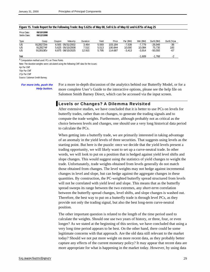
January 31, 2000 Principles of Principal Components
29
Figure 15. Trade Report for the Following Trade: Buy 5.625s of May 08, Sell 6.5s of May 02 and 6.875s of Aug 25
Price Date: 06/10/1998Settle Date: 06/12/1998
Type Cusip Coupon Maturity Duration Yield Price Par ($M) Mkt ($M) Dur$ ($M) Dur$ (%)aUS 9128272W 6.500 05/31/2002 3.464 5.593 103.184 -7,539 -7,779 -26,948 -36US 9128274F 5.625 05/15/2008 7.510 5.513 100.844 10,000 10,084 75,735 100US 912810EV 6.875 08/15/2025 12.915 5.795 114.687 -3,413 -3,914 -50,555 -67
Net -1,609 -1,768 -2a Computation method used: PCs on Three Points
Note: The duration weights were calculated using the following CMT data for the issues:
4yr Par CMT
10yr Par CMT
27yr Par CMT
Source: Salomon Smith Barney.
For a more in-depth discussion of the analytics behind our Butterfly Model, or for amore complete User’s Guide to the interactive options, please see the help file onSalomon Smith Barney Direct, which can be accessed via the input screen.
Levels or Changes? A Dilemma RevisitedAfter extensive studies, we have concluded that it is better to use PCs on levels forbutterfly trades, rather than on changes, to generate the trading signals and tocompute the trade weights. Furthermore, although probably not as critical as thechoice between levels and changes, one should use a very long historical data periodto calculate the PCs.
When getting into a butterfly trade, we are primarily interested in taking advantageof an anomaly in the yield levels of three securities. That suggests using levels as thestarting point. But here is the puzzle: once we decide that the yield levels present atrading opportunity, we will likely want to set up a curve-neutral trade. In otherwords, we will look to put on a position that is hedged against yield level shifts andslope changes. This would suggest using the statistics of yield changes to weight thetrade. Unfortunately, trade weights obtained from levels generally do not matchthose obtained from changes. The level weights may not hedge against incrementalchanges in level and slope, but can hedge against the aggregate changes in thesequantities. By construction, the PC-weighted butterfly spread structured from levelswill not be correlated with yield level and slope. This means that as the butterflyspread sweeps its range between the two extremes, any short-term correlationbetween the butterfly spread changes, level shifts, and slope changes is washed out.Therefore, the best way to put on a butterfly trade is through level PCs, as theyprovide not only the trading signal, but also the best long-term curve-neutralposition.
The other important question is related to the length of the time period used tocalculate the weights. Should one use two years of history, or three, four, or evenlonger? As we stated at the beginning of this section, we have concluded that using avery long time period appears to be best. On the other hand, there could be somelegitimate concerns with that approach. Are the old data still relevant to the markettoday? Should we not put more weight on more recent data, as they probably bettercapture any effects of the current monetary policy? It may appear that recent data aremore appropriate for what is happening in the market today. However, by using data
For more info, push theHelp button.
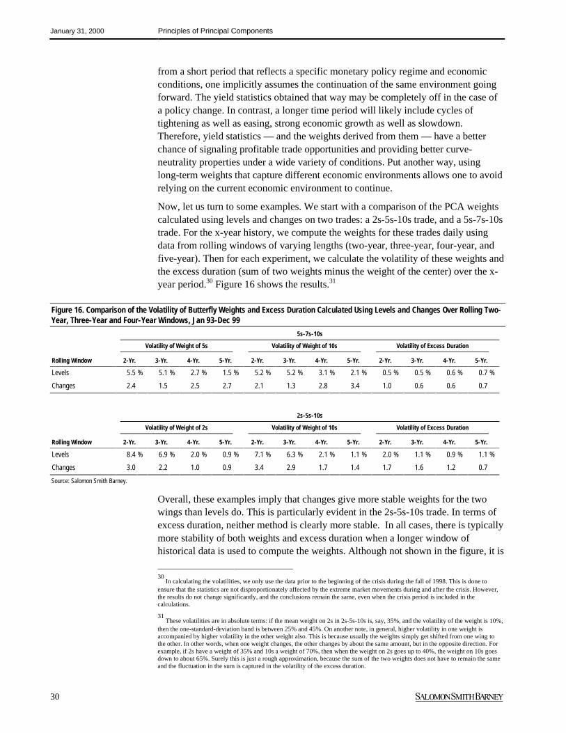
January 31, 2000 Principles of Principal Components
30
from a short period that reflects a specific monetary policy regime and economicconditions, one implicitly assumes the continuation of the same environment goingforward. The yield statistics obtained that way may be completely off in the case ofa policy change. In contrast, a longer time period will likely include cycles oftightening as well as easing, strong economic growth as well as slowdown.Therefore, yield statistics — and the weights derived from them — have a betterchance of signaling profitable trade opportunities and providing better curve-neutrality properties under a wide variety of conditions. Put another way, usinglong-term weights that capture different economic environments allows one to avoidrelying on the current economic environment to continue.
Now, let us turn to some examples. We start with a comparison of the PCA weightscalculated using levels and changes on two trades: a 2s-5s-10s trade, and a 5s-7s-10strade. For the x-year history, we compute the weights for these trades daily usingdata from rolling windows of varying lengths (two-year, three-year, four-year, andfive-year). Then for each experiment, we calculate the volatility of these weights andthe excess duration (sum of two weights minus the weight of the center) over the x-year period.30 Figure 16 shows the results.31
Figure 16. Comparison of the Volatility of Butterfly Weights and Excess Duration Calculated Using Levels and Changes Over Rolling Two-Year, Three-Year and Four-Year Windows, Jan 93-Dec 99
5s-7s-10s
Volatility of Weight of 5s Volatility of Weight of 10s Volatility of Excess Duration
Rolling Window 2-Yr. 3-Yr. 4-Yr. 5-Yr. 2-Yr. 3-Yr. 4-Yr. 5-Yr. 2-Yr. 3-Yr. 4-Yr. 5-Yr.
Levels 5.5 % 5.1 % 2.7 % 1.5 % 5.2 % 5.2 % 3.1 % 2.1 % 0.5 % 0.5 % 0.6 % 0.7 %
Changes 2.4 1.5 2.5 2.7 2.1 1.3 2.8 3.4 1.0 0.6 0.6 0.7
2s-5s-10s
Volatility of Weight of 2s Volatility of Weight of 10s Volatility of Excess Duration
Rolling Window 2-Yr. 3-Yr. 4-Yr. 5-Yr. 2-Yr. 3-Yr. 4-Yr. 5-Yr. 2-Yr. 3-Yr. 4-Yr. 5-Yr.
Levels 8.4 % 6.9 % 2.0 % 0.9 % 7.1 % 6.3 % 2.1 % 1.1 % 2.0 % 1.1 % 0.9 % 1.1 %
Changes 3.0 2.2 1.0 0.9 3.4 2.9 1.7 1.4 1.7 1.6 1.2 0.7
Source: Salomon Smith Barney.
Overall, these examples imply that changes give more stable weights for the twowings than levels do. This is particularly evident in the 2s-5s-10s trade. In terms ofexcess duration, neither method is clearly more stable. In all cases, there is typicallymore stability of both weights and excess duration when a longer window ofhistorical data is used to compute the weights. Although not shown in the figure, it is
30
In calculating the volatilities, we only use the data prior to the beginning of the crisis during the fall of 1998. This is done toensure that the statistics are not disproportionately affected by the extreme market movements during and after the crisis. However,the results do not change significantly, and the conclusions remain the same, even when the crisis period is included in thecalculations.
31 These volatilities are in absolute terms: if the mean weight on 2s in 2s-5s-10s is, say, 35%, and the volatility of the weight is 10%,
then the one-standard-deviation band is between 25% and 45%. On another note, in general, higher volatility in one weight isaccompanied by higher volatility in the other weight also. This is because usually the weights simply get shifted from one wing tothe other. In other words, when one weight changes, the other changes by about the same amount, but in the opposite direction. Forexample, if 2s have a weight of 35% and 10s a weight of 70%, then when the weight on 2s goes up to 40%, the weight on 10s goesdown to about 65%. Surely this is just a rough approximation, because the sum of the two weights does not have to remain the sameand the fluctuation in the sum is captured in the volatility of the excess duration.
January 31, 2000 Principles of Principal Components
31
also interesting that the long-term mean of each weight appears to remain the same,independent of the length of time used to calculate the weights. This suggests thateven though a shorter window may result in higher volatility of weights, the averageweights are consistent with weights obtained from longer periods.
Although stability of the weights is desirable, it is not necessarily the goal. A bettergauge of the effectiveness of the butterfly weights is whether the tradesrecommended and structured by the model generate profits. To test the efficacy ofthe model, we ran historical simulations. We used the change in the butterfly spreadas a measure of the P&L. For example, if we put on a long trade (long the center,short the wings) and the butterfly spread decreases by 1bp, then we make a profit of1bp times the duration dollars in the center of the trade. Conversely, a short trade(short the center, long the wings) makes a 1bp profit if the spread increases by 1bp.
Here is how the simulations work. The trading signals are obtained from thepercentiles of the (PC-weighted) butterfly spread over a rolling window of aspecified length (two-year, 3-year, etc.). Whenever the model indicates that thebutterfly spread is at a low (high) percentile, called the start level, we put on a short(long) trade. Then when the spread reverts back to a higher (lower) level, called theexit level, we take off the trade. The reversion to the exit level is meaningful only ifit does not take too long to happen. So, we put a limit on the maximum number ofdays we would be willing to keep the trade on (the holding period); if the reversionhas not happened by then, we take off the trade, regardless of the P&L situation.That way, we get out of any trade within a reasonable amount of time, and then weare free to put on other trades if opportunities arise.
Before running the simulations to compare levels and changes, we have testedseveral different combinations of start and exit levels, and holding periods tooptimize the choice of these parameters. The results are shown in Figure 17. Thestart and exit levels are in the leftmost column. For example, the first set of start/exitvalues is 3/10, indicating that we put on a short trade when the spread dips below3% (or a long trade, when the spread exceeds 97% ), and take it off when the spreadreverts to the 10% level (or the 90% level). We tried three different holding periodsof 60, 120, and 365 days.
The first observation is that waiting up to 365 days to end a trade results in poorperformance. The second observation is that the higher P&Ls and Sharpe ratios areconcentrated in the upper part of the table, with start/exit percentiles of 3/10, 3/30,and perhaps 10/30. This leads us to believe that the P&L on these trades is realizedat the tail ends of the spread range, and that there is no advantage in looking fortrading signals in the intermediate percentiles. In choosing between using 3% or10% as the level to put on a trade, we note that while the 10% level gives rise tomore trades, the mean P&Ls are not higher, and the Sharpe ratios are decidedlylower than with 3%. Therefore, we favor the 3% level to start the trades. As for thechoice between using 10% or 30% as the exit level, we prefer 30%, due to the higheraverage P&Ls; besides, the Sharpe ratios for 30%, while lower than those for 10%,are still fairly good.

January 31, 2000 Principles of Principal Components
32
Figure 17. Performance of 2s-5s-10s Trade Structured Using Yield Levels for Various Start/Exit Levels and Maximum Holding Periods of60, 120, and 365 Days, Jan 93-Dec 99
Percentage of Trades Taken
Start/Exit No. of Trades Probability of Success Off at Day Limit Mean P & L Volatility of P & L Sharpe Ratio
Levels 60 120 365 60 120 365 60 120 365 60 120 365 60 120 365 60 120 365
3/10
2-Year 20 17 16 85% 88% 94% 30% 18% 6% 2.1bp 1.9bp 1.4bp 2.6bp 3.6bp 7.2bp 0.81 0.53 0.19
3-Year 17 14 12 82 86 100 24 21 0 2.4 2.4 3.5 1.9 2.1 2.0 1.26 1.14 1.75
4-Year 14 12 12 86 100 100 14 0 0 3.1 3.6 3.6 3.5 2.7 2.7 0.89 1.33 1.33
3/30
2-Year 18 14 8 83% 79% 62% 50% 43% 38% 2.2bp 1.4bp -0.5bp 3.0bp 4.3bp 10.5bp 0.73 0.33-0.05
3-Year 16 12 9 81 75 89 62 42 11 2.7 2.9 4.8 2.7 3.5 3.3 1.00 0.83 1.45
4-Year 13 9 6 85 89 83 62 33 17 4.2 5.6 6.6 5.0 5.4 6.5 0.84 1.04 1.02
10/30
2-Year 29 21 12 72% 76% 75% 48% 43% 25% 1.2bp 1.3bp 0.0bp 2.8bp 3.8bp 8.6bp 0.43 0.34 0.00
3-Year 25 19 14 68 74 93 52 32 14 1.5 2.3 3.3 2.9 3.3 2.6 0.52 0.70 1.27
4-Year 23 15 11 83 80 91 52 40 18 2.9 3.7 4.8 3.9 4.4 4.7 0.74 0.84 1.02
10/50
2-Year 28 17 10 64% 65% 70% 68% 59% 30% 1.2bp 1.0bp -0.1bp 3.5bp 4.8bp 9.6bp 0.34 0.21-0.01
3-Year 24 15 11 62 67 82 62 53 36 2.2 2.2 3.2 3.8 4.6 4.5 0.58 0.48 0.71
4-Year 21 15 10 71 73 90 71 53 20 3.0 3.6 5.9 5.1 5.9 6.0 0.59 0.61 0.98
30/50
2-Year 38 25 12 58% 60% 67% 63% 44% 33% 0.4bp 0.6bp -1.5bp 3.4bp 5.2bp 10.6bp 0.12 0.12-0.14
3-Year 38 24 15 55 62 73 66 50 27 1.4 2.1 2.8 3.6 4.4 5.0 0.39 0.48 0.56
4-Year 39 27 19 62 70 79 59 37 21 1.9 3.1 3.8 4.3 5.0 4.9 0.44 0.62 0.78
Source: Salomon Smith Barney.
Next, we ran the simulations to compare levels versus changes. We used the rollingPC weights indicated by the yield levels and yield changes over two-year, three-year, and four-year periods. We also computed the PC weights over an 11-yearperiod — again both for levels and changes — and then went back and applied thosefixed weights over rolling two-year windows during the same 11-year period. This isdifferent from the other simulations, in that it is an in-sample test. Finally, wecomputed butterfly weights, such that we are hedged to the first two PCs of theentire yield curve.32 Figure 18 shows the performance of the trades for each one ofthe different ways of weighting.
32
For example, for the 2s-5s-10s trade, the yield changes implied by the first two PCs (in bp) are 28.4, 30.5, 28.7 and -13.5, -7.1,0.5. A weighting vector that hedges out the first two PCs is orthogonal to these two 3x1 vectors, and is given by the vector product ofthe two vectors. Then we normalize the resulting orthogonal vector such that its weight on 5s is 100%. The final result is -54.5%weight on 2s, 100% on 5s, and -52.3% on 10s.
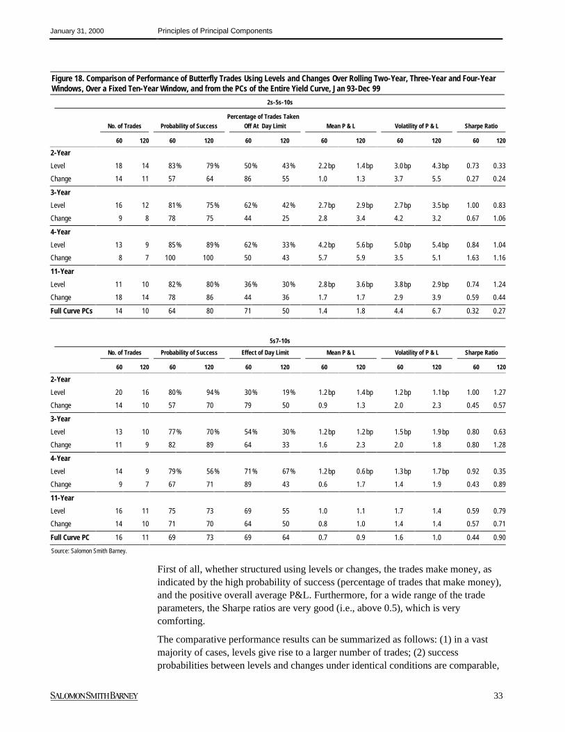
January 31, 2000 Principles of Principal Components
33
Figure 18. Comparison of Performance of Butterfly Trades Using Levels and Changes Over Rolling Two-Year, Three-Year and Four-YearWindows, Over a Fixed Ten-Year Window, and from the PCs of the Entire Yield Curve, Jan 93-Dec 99
2s-5s-10s
Percentage of Trades TakenNo. of Trades Probability of Success Off At Day Limit Mean P & L Volatility of P & L Sharpe Ratio
60 120 60 120 60 120 60 120 60 120 60 120
2-Year
Level 18 14 83% 79% 50% 43% 2.2bp 1.4bp 3.0bp 4.3bp 0.73 0.33
Change 14 11 57 64 86 55 1.0 1.3 3.7 5.5 0.27 0.24
3-Year
Level 16 12 81% 75% 62% 42% 2.7bp 2.9bp 2.7bp 3.5bp 1.00 0.83
Change 9 8 78 75 44 25 2.8 3.4 4.2 3.2 0.67 1.06
4-Year
Level 13 9 85% 89% 62% 33% 4.2bp 5.6bp 5.0bp 5.4bp 0.84 1.04
Change 8 7 100 100 50 43 5.7 5.9 3.5 5.1 1.63 1.16
11-Year
Level 11 10 82% 80% 36% 30% 2.8bp 3.6bp 3.8bp 2.9bp 0.74 1.24
Change 18 14 78 86 44 36 1.7 1.7 2.9 3.9 0.59 0.44
Full Curve PCs 14 10 64 80 71 50 1.4 1.8 4.4 6.7 0.32 0.27
5s7-10s
No. of Trades Probability of Success Effect of Day Limit Mean P & L Volatility of P & L Sharpe Ratio
60 120 60 120 60 120 60 120 60 120 60 120
2-Year
Level 20 16 80% 94% 30% 19% 1.2bp 1.4bp 1.2bp 1.1bp 1.00 1.27
Change 14 10 57 70 79 50 0.9 1.3 2.0 2.3 0.45 0.57
3-Year
Level 13 10 77% 70% 54% 30% 1.2bp 1.2bp 1.5bp 1.9bp 0.80 0.63
Change 11 9 82 89 64 33 1.6 2.3 2.0 1.8 0.80 1.28
4-Year
Level 14 9 79% 56% 71% 67% 1.2bp 0.6bp 1.3bp 1.7bp 0.92 0.35
Change 9 7 67 71 89 43 0.6 1.7 1.4 1.9 0.43 0.89
11-Year
Level 16 11 75 73 69 55 1.0 1.1 1.7 1.4 0.59 0.79
Change 14 10 71 70 64 50 0.8 1.0 1.4 1.4 0.57 0.71
Full Curve PC 16 11 69 73 69 64 0.7 0.9 1.6 1.0 0.44 0.90
Source: Salomon Smith Barney.
First of all, whether structured using levels or changes, the trades make money, asindicated by the high probability of success (percentage of trades that make money),and the positive overall average P&L. Furthermore, for a wide range of the tradeparameters, the Sharpe ratios are very good (i.e., above 0.5), which is verycomforting.
The comparative performance results can be summarized as follows: (1) in a vastmajority of cases, levels give rise to a larger number of trades; (2) successprobabilities between levels and changes under identical conditions are comparable,
January 31, 2000 Principles of Principal Components
34
and typically high (upward of 70%) especially if a long window is used; (3) in fiveout of eight cases for 2s-5s-10s and six out of eight cases for 5s-7s-10s, levels havesame or better Sharpe ratios than changes; (4) longer time windows appear to boostaverage P&L for 2s-5s-10s, but not so for 5s-7s-10s, but there is no advantage inusing the 11-year history (instead of say, the three-year history), even though theresults of the 11-year case are in-sample; (5) waiting longer (120 days instead of 60)for the profit potential to be realized may increase average P&L, but at the expenseof higher volatility, so Sharpe ratios do not necessarily improve; (6) the trades thatuse weights from PCs of the entire yield curve have the worst performance,indicating that specific trades are better managed using PCs that are tailor-made forthose trades, rather than by the generic ones for the curve.
As a result of these observations, the choice between levels and changes is still atough one, but we opt for levels for two reasons: the higher number of trades and the(generally) higher Sharpe ratios. Because the average P&L does not improvedrastically by increasing the holding period for trades, and the Sharpe ratios areacceptable across the board, we prefer a shorter holding period (60 days in thisstudy) so that we have more trades. Finally, regarding the length of the window, weprefer longer windows (three years or longer), due to the higher average P&Ls, asSharpe ratios are fairly high using levels and a 60-day maximum holding period nomatter what the window length. However, we should caution against using a verylong period (11 years, in our study), because there does not seem to be an advantagein terms of P&L and the number of trades.
An interesting question is whether levels and changes give the same trading signals,i.e., whether the timing of the trades is identical. The answer is no: in a majority ofcases, the two approaches give different trading signals. The average P&L of the 2s-5s-10s trade is a respectable 4bp or 5bp if the trades are structured with levels in theoptimal way. However, the 5-7s-10s trade has an average P&L of about 1bp withlevels, no matter what the length of the time window used. So, one could naturallyask whether this is a worthwhile trade, especially taking into account the bid-offerspread. We should emphasize that our historical simulations are based on CMT yielddata derived from our Treasury model. Therefore, what our results establish is asimple proof of concept: the model makes money. In reality, one would set up thesetrades with actual issues, and ideally sell issues that are rich (to the model) and buythose that are cheap. That could easily add another few basis points to each trade.Furthermore, our CMT data come from closing prices. But during a trading day,there can be large fluctuations in the butterfly spread — because of an economicannouncement, for instance — that can create very good trading opportunities.Because investors quickly take advantage of such extreme relative valueopportunities, these opportunities disappear just as quickly, usually before the day isover. Finally, P&L can be further boosted by using futures instead of cash.Therefore, our results should be viewed as a conservative estimate of theprofitability of trades structured using the butterfly model.
To conclude this section on levels versus changes, we would like to remind ourreaders that PCA ignores the fact that yields are time series. Although we believethat level PCs give a more than adequate answer to timing and setting up a butterfly

January 31, 2000 Principles of Principal Components
35
trade, it is conceivable that the results can be improved further by using a model thatexploits the time series properties of yields. At the very least, such a model wouldput to rest the question of whether to use levels or changes by implicitly combiningthe two in a consistent framework.
Lessons From the Crisis of Fall 1998Before we conclude, we would like to reiterate the importance of using a long-enough time window (three or four years). With a shorter window, periods ofunusual yield curve movements or single monetary policy regimes may affect thestatistics disproportionately. A very important example of this is related to the crisisduring the fall of 1998. In particular, because of the demand for the liquidity of theon-the-run issues, the off-the-run sectors cheapened relative to the on-the-runs andhave not yet fully recovered. As a result, the shape of the curve underwent adramatic change, with a more dominant hump in the 21-year sector than wasobserved previously. The 9s-21s-28s trade demonstrates this effect. Using a two-year history prior to the crisis, PCA would give weights of -5% for the nine-year and-96.7% for the 28-year (the minus signs indicate that these securities are sold againsta purchase of 21s). However, the same analysis at the beginning of November 1999gives +34.3% for the nine-year and -149.3% for the 28-year, i.e., one has to buy thenine-year and sell more of the 28-year to hedge level and slope risk! This is nolonger a butterfly trade. What happened is that with the onset of the crisis, the curvebecame more humped, so the hump (or curvature) started to explain a higherpercentage of the curve shape. Since the first two PCs picked this up, the third PCwas distorted to such an extent that it could not be interpreted as curvature any more.One can still construct a butterfly of 9s-21s-28s, by excluding the crisis period fromthe analysis (e.g. getting the PCA weights from the pre-crisis or post-crisis period).Using nine months of data in the post-crisis period, the weights are -8.3% and-94.9% — much more sensible than the weights from the two-year period includingthe crisis. Another possibility is to use cash-neutral and duration-neutral weights, butthis is likely to be an inferior choice, as it does not make use of the statistics of theyields. The best alternative is to use a longer time window: using a four-yearwindow, the weights do not exhibit those peculiar swings: using pre-crisis data, theweights are -6.6% and -95.4%, compared with -2.8% and -95.8% from the periodincluding the crisis.

January 31, 2000 Principles of Principal Components
36
Appendix A – Computation of the Principal ComponentsLet y1, y2, …, yK be K different (scalar) time series. The value of the nth sample, orobservation, of the kth time series is denoted by yk(n). In our applications, the yKs areyield levels or yield changes at different maturity points. In PCA, for the entire yieldcurve, we have y1 through y120 (K = 120) that represent the time series of 120 CMTpoints spanning the maturity range up to 30 years with quarter-year increments. Forbutterfly applications, we have three time series (K=3) that represent the yields (orchanges) of the securities in the three legs of the trade.
Let y(n) denote the value of the Kx1 vector of the K time series y1, y2, …, yK, at timen, i.e.
=
)(
)(
)(
)( 2
1
ny
ny
ny
n
K
My
Being a vector in a K-dimensional space, y(n) can be written in terms of a given(fixed) set of K orthonormal33 Kx1 vectors a1, a2, …, aK
KK ncncncn aaay )()()()( 2211 +++= L
for some scalar coefficients c1(n), c2(n), …, cK(n). Because the aks are orthonormal,for each y(n) there is a distinct and unique set of coefficients c1(n), c2(n), …, cK(n)that satisfy the equation above. These coefficients are given by
,)()( kT
k nnc ay= for Kk ,,1L=
Clearly, the value of the coefficients c1(n), c2(n), …, cK(n) for a given y(n) dependson the choice of ak.
Given N observations of the Kx1 vector y, denoted by y(1), y(2), …, y(N), one cancalculate a coefficient ck(n) for each observation y(n). This gives, in effect, Nobservations of the coefficient ck. Given these N observations, it is a simple matter tocalculate the variance of each coefficient ck.
The objective in principal components analysis is to find a set of orthonormal a’ssuch that the first coefficient c1 has the largest variance possible for any choice of a1,the second coefficient c2 has the second-largest variance, and so on. The problem offinding a1 that gives the highest variance reduces to the following form:
maximize 11 aa ST subject to 111 =aaT ,
where S is the covariance matrix of y. The solution to this constrained optimizationproblem is given by the eigenvector of S associated with the largest eigenvalue. Infact, the highest variance thus found is the largest eigenvalue. Similarly, a2 is thesolution to the problem
33
An orthonormal set of vectors a1, a
2, …, a
K satisfies two properties: i) the vectors have unity vector norm, and ii) the vectors are
orthogonal to each other.
January 31, 2000 Principles of Principal Components
37
maximize 22 aa ST subject to 122 =aaT and 012 =aaT
and is given by the eigenvector of S associated with the second-largest eigenvalue.Again, the second largest variance turns out to be equal to the second-largesteigenvalue. The remaining orthonormal vectors a3, …, aK are computed in a similarway. The vectors a1 ,…, aK are called loadings and the coefficients c1, c2, …, cK arecalled principal components (note that in this report, we refer to the vectors looselyas principal components to reduce the statistical jargon).
The importance of principal components is that a large part of the variance in thevector y can be explained by a relatively small number of principal components. Thefundamental relationship is the following:
∑∑==
=K
kk
K
kk cVaryVar
11
)()(
In other words, the total variance in the vector y is equal to the sum of the variancesof the principal components, i.e., each principal component explains part of the totalvariance. In our yield curve PCA application, the first three principal components(the ones associated with the largest eigenvalues) explain 99.4% of the totalvariance. In contrast, in the butterfly application, there are three yield time series(K=3), so the first three PCs are the only PCs and as such they represent all of thevariance.
Appendix B – Methodologies for Computing PortfolioHedges Using Principal Components34
Computing the Independent TradesWe suggest two methods for computing the Independent Trades that represent thethree PCs. Fundamental to both methods is the selection of the hedge securities andthe calculation of scenario dollar returns in the Yield Book™. We have concludedthat the best hedges occur when the three securities are “well-spaced” along thecurve and are representative of the portfolio being hedged. Because we will be usingthese independent trades to hedge the Treasury Index, we have selected the on-the-run two, ten, and 30-year Treasury issues. We suggest using the one-month PCscenarios ("pc1mo" scenario file) in the Yield Book™. This scenario file containssix scenarios, two for each PC: for example comp1+ and comp1- are the respectivepositive and negative realizations of the first component. These scenarios are scaledto the appropriate one-month one-standard-deviation for each component. Calculatereturns using a zero-day horizon.
1 Analytic solution for computing the Independent Trades. This approach utilizesanalytic and algebraic techniques to construct the three Independent Trades. First,we need the sensitivities of each hedge security to each PC. Using the YieldBook™, calculate scenario dollar returns for the one-month horizon PCscenarios. The sensitivity of an issue to the first component equals the dollarreturn under comp1+ minus the dollar return under comp1-, divided by two.Similar calculations are done for the other components. The next step is to solve
34
Parts of this appendix originally appeared in the March 6, 1998, issue of Bond Market Roundup: Strategy, Salomon Smith Barney.

January 31, 2000 Principles of Principal Components
38
a system of linear equations to determine each Independent Trade. Thecoefficients in this system are the PC sensitivities, and the unknowns are thetrade weights for each security. The system of equations is defined in such a waythat the solution set of trade weights produces a portfolio with exposure to onlyone component at a time. 35 It is worth mentioning that such a system is well-defined and has a unique solution, since the PCs are independent by constructionand we are using three hedging securities to hedge out the three exposures.
2 Optimization solution for computing Independent Trades. Using the optimizationfeature of the Yield Book™ on chapter 4, pg. 2, the weights for each IndependentTrade can be easily obtained. Bring in the three hedge securities onto both thebuy and sell sides.36 Once the scenario returns have been calculated, performthree optimizations — one for each Independent Trade, as follows. Enter theobjective and constraints of the optimization: Constrain the dollar returndifferences of the positive PC scenarios (one will be positive and two zero) and“maxmin” over the negative PC scenarios. For example, to calculate theIndependent Trade to hedge the first component (a level shift of the yield curve),constrain the dollar return difference of the first scenario, comp1+, to someamount, say $1 million, set the dollar-return difference of comp2+ and comp3+equal to zero and “maxmin” the dollar-return differences of comp1-, comp2-, andcomp3-.37 Repeat for comp2+ (a change in slope) and comp3+ (a change incurvature).
35
For each i=1, 2, 3, solve: W(1)*S(1,k)+ W(2)*S(2,k)+ W(3)*S(3,k)=E(i), where E(i)=1 if i=k and 0 otherwise, where S are thesensitivities, W are the security weights and E the exposures to each component.
36 Since we do not know a priori whether the solution will be short or long each issue.
37 Because of convexity, constraining comp1+ to be 1,000 and comp1- to be 1,000 and the other return differences to be zero will
not produce a feasible solution.

January 31, 2000 Principles of Principal Components
39
Figure 19. Independent Hedge Trades for $1 Million Exposure to a One-Month One-Standard-DeviationMove in Each Component (Market Value in $ Thousands), 27 Feb 98
Analytic Solution Yield Book Optimization SolutionIndependent Trade 1 -- Level
Market MarketEDUR$ Weight Value EDUR$ Weight Value
2-Year -$5,686 15.42% -$30,537 -$5,768 15.38% -$30,97610-Year -16,735 45.40 -22,033 -17,021 45.38 -22,40930-Year -14,442 39.18 -10,600 -14,715 39.24 -10,800
-$36,863 100.00% -$37,503 100.00%Independent Trade 2 -- Slope
EDUR$ Weight EDUR$ Weight 2-Year $57,281 100.00% $307,633 $57,051 100.00% $306,39510-Year -14,480 -25.28 -19,064 -15,010 -26.31 -19,76230-Year -49,055 -85.64 -36,004 -49,584 -86.91 -36,392
-6,254 -10.92% -$7,543 -13.22%Independent Trade 3 -- Curvature
EDUR$ Weight EDUR$ Weight 2-Year -$71,838 -25.14% -$385,813 -$71,854 -25.25% -$385,89910-Year 285,769 100.00 376,235 284,535 100.00 374,61130-Year -248,715 -87.03 -182,544 -249,858 -87.81 -183,383
-34,784 -12.17% -$37,177 -13.07%Source: Salomon Smith Barney.
In Figure 19, we show the size of each trade that will provide a $1 million profit(exposure) to a one-standard-deviation move (over a one-month period) in eachcomponent for both methods. These trades each have exposure to only one PC andprovide an intuitive meaning of the nature of the three PCs. These two proceduresreturn nearly identical solutions.
Computing Portfolio HedgesFor computing hedges of a portfolio, we suggest four possible methods:
1 Calculate the hedge from the Independent Trades that have been calculatedvia one of the methods above. Here, the Yield Book™ can be used to the dollarsensitivities of the portfolio, or index, to the three components through scenarioanalysis with our "pc1mo" scenario file. Since each Independent Trade createsexposure to only one component, each trade can be sized to offset the portfolio'sdollar sensitivity to the corresponding component.38 These three sized trades canthen be aggregated to determine the amounts of the three securities thatcomprise the hedge. Figure 20 displays the hedge for the Treasury Indexresulting from the scaling of the Independent Trades created through theoptimization method (method 2) detailed above.
38
Simply scale the market values in each Independent Trade by the portfolio’s dollar exposure to a component divided by $1million.
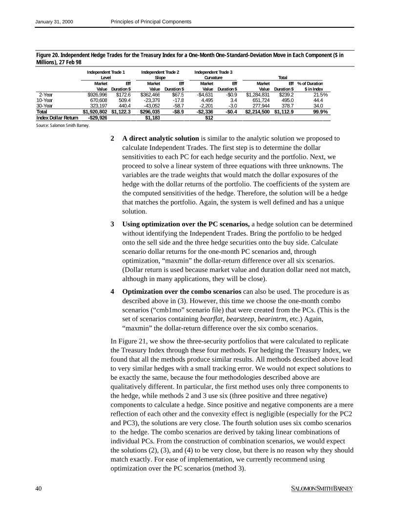
January 31, 2000 Principles of Principal Components
40
Figure 20. Independent Hedge Trades for the Treasury Index for a One-Month One-Standard-Deviation Move in Each Component ($ inMillions), 27 Feb 98
Independent Trade 1 Independent Trade 2 Independent Trade 3Level Slope Curvature Total
Market Eff Market Eff Market Eff Market Eff % of DurationValue Duration $ Value Duration $ Value Duration $ Value Duration $ $ in Index
2-Year $926,996 $172.6 $362,466 $67.5 -$4,631 -$0.9 $1,284,831 $239.2 21.5%10-Year 670,608 509.4 -23,379 -17.8 4,495 3.4 651,724 495.0 44.430-Year 323,197 440.4 -43,052 -58.7 -2,201 -3.0 277,944 378.7 34.0Total $1,920,802 $1,122.3 $296,035 -$8.9 -$2,336 -$0.4 $2,214,500 $1,112.9 99.9%Index Dollar Return -$29,926 $1,183 $12Source: Salomon Smith Barney.
2 A direct analytic solution is similar to the analytic solution we proposed tocalculate Independent Trades. The first step is to determine the dollarsensitivities to each PC for each hedge security and the portfolio. Next, weproceed to solve a linear system of three equations with three unknowns. Thevariables are the trade weights that would match the dollar exposures of thehedge with the dollar returns of the portfolio. The coefficients of the system arethe computed sensitivities of the hedge. Therefore, the solution will be a hedgethat matches the portfolio. Again, the system is well defined and has a uniquesolution.
3 Using optimization over the PC scenarios, a hedge solution can be determinedwithout identifying the Independent Trades. Bring the portfolio to be hedgedonto the sell side and the three hedge securities onto the buy side. Calculatescenario dollar returns for the one-month PC scenarios and, throughoptimization, “maxmin” the dollar-return difference over all six scenarios.(Dollar return is used because market value and duration dollar need not match,although in many applications, they will be close).
4 Optimization over the combo scenarios can also be used. The procedure is asdescribed above in (3). However, this time we choose the one-month comboscenarios (“cmb1mo” scenario file) that were created from the PCs. (This is theset of scenarios containing bearflat, bearsteep, bearintrm, etc.) Again,“maxmin” the dollar-return difference over the six combo scenarios.
In Figure 21, we show the three-security portfolios that were calculated to replicatethe Treasury Index through these four methods. For hedging the Treasury Index, wefound that all the methods produce similar results. All methods described above leadto very similar hedges with a small tracking error. We would not expect solutions tobe exactly the same, because the four methodologies described above arequalitatively different. In particular, the first method uses only three components tothe hedge, while methods 2 and 3 use six (three positive and three negative)components to calculate a hedge. Since positive and negative components are a merereflection of each other and the convexity effect is negligible (especially for the PC2and PC3), the solutions are very close. The fourth solution uses six combo scenariosto the hedge. The combo scenarios are derived by taking linear combinations ofindividual PCs. From the construction of combination scenarios, we would expectthe solutions (2), (3), and (4) to be very close, but there is no reason why they shouldmatch exactly. For ease of implementation, we currently recommend usingoptimization over the PC scenarios (method 3).

January 31, 2000 Principles of Principal Components
41
Figure 21. Hedge Trades for the Treasury Index for a One-Month One-Standard-Deviation Move in Each Component ($ in Millions), 27 Feb98
Independent Trades Analytic Solution PC Optimization Combo OptimizationMarket Val. %EDUR$ Market Val. %EDUR$ Market Val. %EDUR$ Market Val. %EDUR$
2-Year $1,284,831 21.50% $1,284,118 21.49% $1,284,991 21.50% $1,281,059 21.44%10-Year 651,724 44.48 651,749 44.49 651,437 44.46 653,621 44.6230-Year 277,944 34.03 277,863 34.02 278,115 34.05 277,230 33.95
$2,214,500 100.00% $2,213,730 100.00% $2,214,543 100.01% $2,211,910 100.01%Source: Salomon Smith Barney.
Hedging a Portfolio Versus an IndexTaking our analysis one step further, if you have a portfolio that is benchmarkedagainst the Treasury Index and you would like to see if it is well hedged formovements in the Treasury yield curve, the following can be done:
1 Scale the market value of the index to equal the market value of your portfolio.Compute the hedges for the index and your portfolio, separately, under one of themethods detailed above. You will then have two portfolios of three securitiesapiece that can be compared to determine what trades, if any, need to be put on tomatch the exposures of the index.
2 Bring your portfolio onto the buy side and the index onto the sell side. Again,scale the market value of the index to that of your portfolio. Bring in the selectedhedge securities onto both the buy and sell sides and use method 3 or 4(optimization over PC or combo scenarios). Any additional securities on the buyside and/or the sell side represent trades that will neutralize the exposures of theportfolio versus the Index for those scenarios.
Appendix C – What Is the “Right” Butterfly Spread toAssess Performance in a Butterfly Trade?39
Our butterfly model allows investors to identify rich and cheap sectors of the curveand to set up curve-neutral butterfly trades to take advantage of these relative-valueopportunities. The optimal allocation of the duration-dollars in the trade is calculatedautomatically by the model, based on the objectives and constraints specified by theinvestor. Discussions with users of our butterfly model often raise the issue thatmany investors follow 50-50 weighted butterfly spreads, which may not accuratelytrack the performance of these trades. We provide an overview of the spreads thatultimately are related to the P&L of the trade.
The value in a butterfly trade lies in the relative cheapness or richness of a bulletagainst a barbell. An opportunity exists when the shape defined by the yields of thethree securities is more humped than observed in historical data: In this case, aninvestor would want to own the bullet and sell the barbell. Conversely, when theshape has much less of a kink than in the past (or a more pronounced negative kink),it means that the bullet is rich relative to the barbell, and one would sell the bulletand buy the barbell.
The return on the butterfly trade is due to two factors:40
39
The material in this appendix originally appeared in the March 12, 1999 issue of Bond Market Roundup: Strategy.
40 This analysis is linear and ignores the effect of convexity.

January 31, 2000 Principles of Principal Components
42
The yield on the composite position, and
The change in yields of the three securities.
The short-term relative-value investor expects to benefit primarily from the secondfactor, as a result of a change in the “spread” between the bullet and the barbell.Here the spread is understood to be a measure of the curvature of the three yields.The market convention is to quote this spread on a 50-50 basis.41
Market Convention Spread = ( )winglongwingshortbullet yyy +−2
Therefore, when this spread decreases, being long the bullet and short the barbellshould result in a profit. However, unless the duration-dollars are allocated equallybetween the two wings of the barbell (50% in the short wing and 50% in the longwing), the change in this spread is only loosely tied to the actual profit in the trade.
Confounding the issue of the P&L of a butterfly trade is the convention of quotingthe yield pickup on the same 50-50 basis using the above equation. As mentionedabove, the yield pickup on the composite position determines one component of thereturn. However, calculating this component of the return in the trade using thequoted 50-50 yield pickup could again be misleading, unless the total market valuein the barbell is allocated equally between the two wings.
To see how the yield and the butterfly spread should be calculated for an arbitrarybutterfly trade, one can start by reviewing the terms in the return expression for thetrade. First, the change in the value42 P of a bond can be approximated by:
dP P ydt PDdy≅ − .
In this equation, dP is the change in value, D is the duration of the bond, y is theyield, and dy and dt denote the change in yield and time, respectively. The productPD is the duration-dollars in the bond position. The first term on the right is theyield return and the second term is the return due to a change in yield.
The P&L in a butterfly trade is the difference between the change in value of the buyside and the change in value of the sell side. For simplicity, assume that the trade iscash-neutral, i.e., that the market values of the buy and sell sides are the same.43
Denoting this market value by P and the duration-dollars on any leg of the trade byDD, the P&L of a long-bullet/short-barbell trade is given by:
41
yshort wing and ylong wing denote the yields on the short-maturity and long-maturity securities of the barbell, respectively.
42 This analysis is linear and ignores the effect of convexity.
43 If there is a cash mismatch in the trade, the return on the cash should also be included in the return calculations. This cash
component is invested (or borrowed) using short-term instruments. Because of the small duration on these instruments, the return oncash is primarily owing to yield. When the trade is kept on for a short time, this yield return is small but should not be ignored.
The conventional spreadassumes an equal
allocation of theduration-dollars between
the two wings.
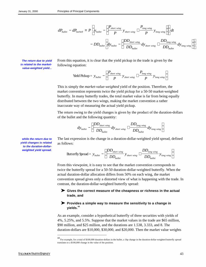
January 31, 2000 Principles of Principal Components
43
dP dP P yP
Py
P
Py dt
DD dyDD
DDdy
DD
DDdy
bullet barbell bullet
short wing
short wing
long wing
long wing
bullet bullet
short wing
bulletshort wing
long wing
bulletlong wing
− = − +
− − +
From this equation, it is clear that the yield pickup in the trade is given by thefollowing equation:
Yield Pickup = yP
Py
P
Pybullet
short wing
short wing
long wing
long wing− +
This is simply the market-value-weighted yield of the position. Therefore, themarket convention represents twice the yield pickup for a 50-50 market-weightedbutterfly. In many butterfly trades, the total market value is far from being equallydistributed between the two wings, making the market convention a ratherinaccurate way of measuring the actual yield pickup.
The return owing to the yield changes is given by the product of the duration-dollarsof the bullet and the following quantity:
dyDD
DDdy
DD
DDdybullet
short wing
bulletshort wing
long wing
bulletlong wing− +
The last expression is the change in a duration-dollar-weighted yield spread, definedas follows:
Butterfly Spread = yDD
DDy
DD
DDybullet
short wing
bulletshort wing
long wing
bulletlong wing− +
From this viewpoint, it is easy to see that the market convention corresponds totwice the butterfly spread for a 50-50 duration-dollar-weighted butterfly. When theactual duration-dollar allocation differs from 50% on each wing, the marketconvention spread gives only a distorted view of what is happening with the trade. Incontrast, the duration-dollar-weighted butterfly spread:
➤ Gives the correct measure of the cheapness or richness in the actualtrade, and
➤ Provides a simple way to measure the sensitivity to a change inyields.44
As an example, consider a hypothetical butterfly of three securities with yields of4%, 5.25%, and 5.5%. Suppose that the market values in the trade are $65 million,$90 million, and $25 million, and the durations are 1.538, 3.333, and 8. Theduration-dollars are $10,000, $30,000, and $20,000. Then the market value weights
44
For example, for a total of $100,000 duration-dollars in the bullet, a 1bp change in the duration-dollar-weighted butterfly spreadtranslates to a $100,000 change in the value of the position.
The return due to yieldis related to the market-
value-weighted yield...
while the return due toyield changes is related
to the duration-dollar-weighted yield spread.
January 31, 2000 Principles of Principal Components
44
are 65/90 = 72.2% and 25/90 = 27.8% for the short wing and long wing,respectively. The duration-dollar weights, on the other hand, are 10/30 = 33.3% and20/30 = 66.7%. Therefore, the yield pickup is 83.3bp (= 5.25 - (0.722*4 +0.278*5.5) = 0.833%) and the duration-dollar-weighted butterfly spread is 25bp (=5.25 - (0.333*4 + 0.667*5.5) = 0.25%). However, one half of the 50-50 spread is50bp.
Not only are all these spreads different levels, providing different indications of anyyield pickup in the trade, but as yields change over time the changes in these spreadsare not necessarily correlated. For example, suppose that over a one-week period,the short wing cheapens by 3bp and the long wing richens by 3bp, while the bullet’syield stays the same. This represents a flattening of the curve from the short wing tothe long wing. In this case, the 50-50 spread is unchanged, but the duration-dollar-weighted spread widens by 1bp (= 0 - (0.333*0.03 + 0.667*(-0.03)) = 0.01%). Nowconsider the opposite case, in which the curve steepens from the short wing to thelong wing: the short wing richens by 3bp, the long wing cheapens by 3bp, and thebullet’s yield stays unchanged. The 50-50 spread is still 0bp. However, this time theduration-dollar-weighted spread tightens by 1bp (= 0 - (0.333*(-0.03) + 0.667*0.03)= -0.01%).
We have assumed in this discussion that the trade that is executed is both market-value- and duration-dollar-neutral. However, this is not always the case and, if it isnot, further complications and confusions can arise. When the duration dollars onthe buy and sell sides are equal but cash is needed to make the market values equal,the duration-dollar-weighted spread of the three securities will be correlated withperformance. However, the market-value-weighted yield used in evaluating thereturn due to yield pickup must also include the cash return. This is obviously moreimportant the longer the holding period of the trade. Failure to include the cashreturn could make a winning trade look like a losing trade.
When using our butterfly model to compute weights based on three principalcomponents, trades that are duration-dollar-neutral rarely result. In this case, theformula for the butterfly spread above still holds. However, the weights for the shortand long wings will not add to one, as in the duration-dollar-neutral trade.45
45
While this adds no complication to the application of that formula, it will for investors who compute butterfly spreads byweighting the short spread (yield bullet - yield short wing) and the long spread (yield bullet - long wing) by the weights in the longand short wings. This will no longer result in the same values.
The change in the 50-50spread may not becorrelated with the
changes in the duration-dollar-weighted butterfly
spread.
When the trade is notmarket-value-neutral, thereturn on cash should be
included in the P&L ofthe trade.

ADDITIONAL INFORMATION AVAILABLE UPON REQUEST
For securities recommended in this report, Salomon Smith Barney (SSB), including its parent, subsidiaries, and/or affiliates (the Firm), usually makes a market, maysell to or buy from customers as principal, and may from time to time perform investment banking or other services for or solicit investment banking or otherbusiness from any company mentioned in this report. Securities recommended, offered, or sold by SSB: (i) are not insured by the Federal Deposit InsuranceCorporation; (ii) are not deposits or other obligations of any insured depository institution (including Citibank); and (iii) are subject to investment risks, including thepossible loss of the principal amount invested. The Firm, or any individuals preparing this report, may at any time have a position in any securities or options of anyof the issuers in this report. An employee of the Firm may be a director of a company mentioned in this report.
Although information has been obtained from and is based upon sources SSB believes to be reliable, the Firm does not guarantee the accuracy of the information,and it may be incomplete or condensed. All opinions and estimates included in this report constitute SSB’s judgment as of the date of this report and are subject tochange without notice. This report is for informational purposes only and is not intended as an offer or solicitation with respect to the purchase or sale of anysecurity. This report does not take into account the investment objectives, financial situation, or particular needs of any particular person. Investors should obtainindividual financial advice based on their own particular circumstances before making an investment decision on the basis of the recommendations in this report.Investors who have received this report from the Firm may be prohibited in certain states from purchasing securities mentioned in this report from the Firm. Pleaseask your Financial Consultant for additional details.
This publication has been approved for distribution in the United Kingdom by Salomon Brothers International Limited, which is regulated by the Securities andFutures Authority. The investments and services contained herein are not available to private customers in the UK. This report was prepared by SSB and, ifdistributed by Nikko Salomon Smith Barney Limited, is so distributed under license. This report is made available in Australia through Salomon Smith BarneyAustralia Securities Pty. Ltd. (ACN 003 114 832), a Licensed Securities Dealer, and in New Zealand through Salomon Smith Barney New Zealand Limited, a memberfirm of the New Zealand Stock Exchange.
The research opinions of the Firm may differ from those of The Robinson-Humphrey Company, LLC, a wholly owned brokerage subsidiary of Salomon Smith BarneyInc. Salomon Smith Barney is a service mark of Salomon Smith Barney Inc. © Salomon Smith Barney Inc., 2000. All rights reserved. Any unauthorized use,duplication, or disclosure is prohibited by law and will result in prosecution.
(6254int)FI01A078