Primality Testing Using Elliptic Curves

Primality Testing Using Elliptic Curves

SHAFI GOLDWASSER

Massachusetts Institute of Technology, Cambridge, Massachusetts

AND

JOE KILIAN

NEC Research Institute, Princeton, New Jersey

Abstract. We present a primality proving algorithm—a probabilistic primality test that produces shortcertificates of primality on prime inputs. We prove that the test runs in expected polynomial time forall but a vanishingly small fraction of the primes. As a corollary, we obtain an algorithm forgenerating large certified primes with distribution statistically close to uniform. Under the conjecturethat the gap between consecutive primes is bounded by some polynomial in their size, the test isshown to run in expected polynomial time for all primes, yielding a Las Vegas primality test.

Our test is based on a new methodology for applying group theory to the problem of primecertification, and the application of this methodology using groups generated by elliptic curves overfinite fields.

We note that our methodology and methods have been subsequently used and improved upon,most notably in the primality proving algorithm of Adleman and Huang using hyperelliptic curves andin practical primality provers using elliptic curves.

Categories and Subject Descriptors: F.1.2 [Computation by Abstract Devices]: Modes of Computa-tion; F.2.1 [Analysis of Algorithms and Problem Complexity]: Numerical Algorithms and Problems

General Terms: Algorithms, Theory

Additional Key Words and Phrases: Distribution of primes, elliptic curves, group theory, Las Vegasalgorithms, primes, prime certification, prime generation

The results of this paper appeared first in Proceedings of the 18th Annual ACM Symposium on Theoryof Computing, ACM, New York, 1986, pp. 316 –329, and then in Chapter 2 of the second author’sthesis (KILIAN, J. 1990. Uses of randomness in Algorithms and Protocols. MIT Press, Cambridge,Mass.). This paper is based upon the writeup in the thesis, with major revisions.Research supported by NSF Postdoctoral Fellowship while at the MIT Laboratory for ComputerScience.The work of S. Goldwasser was supported by ARO grant DAAL 03-86-K-0171 and the NationalScience Foundation (NSF) grant 86-57527-CCR.The research of J. Kilian was supported by NSF Postdoctoral Fellowship while at the MIT Laboratoryfor Computer Science.Authors’ addresses: S. Goldwasser, Computer Science Department, Laboratory for ComputerScience,Massachusetts InstituteofTechnology,Cambridge,MA02139,e-mail: [email protected]; J. Kilian, NEC Research Institute, 4 Independence Way, Princeton, NJ 08540.Permission to make digital / hard copy of part or all of this work for personal or classroom use isgranted without fee provided that the copies are not made or distributed for profit or commercialadvantage, the copyright notice, the title of the publication, and its date appear, and notice is giventhat copying is by permission of the Association for Computing Machinery (ACM), Inc. To copyotherwise, to republish, to post on servers, or to redistribute to lists, requires prior specific permissionand / or a fee.© 1999 ACM 0004-5411/99/0700-0450 $05.00

Journal of the ACM, Vol. 46, No. 4, July 1999, pp. 450 –472.

1. Introduction

The written history of distinguishing prime numbers from composites goes backto Eratosthenes who came up with the first recorded algorithm for primalitytesting, in the 3rd century BC. He showed how to efficiently generate the set ofprimes from 1 to N in O(N ln ln N) arithmetic steps.

Starting in the 17th century, mathematicians (Fermat, Euler, Legendre, andGauss, to name a few) began to study primality once more. Their work laid thefoundation for a new age in primality testing, which began in the 1970’s. In thisearly work (see, for example, Brillhart et al. [1975] and Williams [1978]),factoring and primality testing were intimately related. Consequently, the algo-rithms were quite slow or worked for numbers of a special form (Brillhart et al.[1988] follows up on this work on factoring numbers of a particular form). Then,using elementary results from number theory, Miller [1976], Solovay-Strassen[1977], and Rabin [1980] developed efficient (polynomial time) algorithms forthese problems.

Solovay-Strassen [1977] and Rabin [1980] give randomized primality tests. Onan input N, these tests flip a sequence of coins, and compute its answer based onN and the outcome of these coins. If N is composite, the tests will with highprobability output a proof (witness) that N is composite. If N is prime, they willfail to produce a witness of compositeness, giving probabilistic support to theassertion that N is prime, but no definitive proof.

Miller [1976] gives a deterministic polynomial-time algorithm for primalitytesting based on the Extended Riemann Hypothesis (ERH). On input N, thealgorithm searches for a proof that N is composite. If it finds one, it stops andreports that N is composite, along with its proof of compositeness. If it doesn’tfind a proof of compositeness, the algorithm reports that either N is prime or theERH is false. Hence, a proof of the ERH implies the existence of an efficientdeterministic primality test; unfortunately, this proof is not currently withinreach.

Adleman et al. [1983] and Cohen-Lenstra [1984] give nearly polynomial-timedeterministic primality tests that do not rely on any unproven assumptions. Theyrequire ku (ln ln k) computational steps on an input N of length k. Furthermore,they do not provide any succinct proof of the primality number of a number itdeclares prime.

Given the previous success at producing proofs of compositeness, a naturalquestion is whether one can produce short proofs of primality. We call such ashort proof a certificate of primality. Pratt [1975] has shown that such a shortcertificate of primality always exists (and hence that primes are in NP), but whilehis method is constructive it requires one to factor large integers and thus doesnot run in polynomial time. Wunderlich [1983] discusses a heuristic that willefficiently find certificates for some primes; however, the set of primes certifiablein this manner is sparse, and indeed has not been proven to be infinite. However,it turns out that these techniques, albeit in much more general form, are useful inthe efficient generation of certificates of primality for most (probably all) primes.This is the topic of our work.

We present a simple methodology for applying group theory to the problem ofprime certification. We use this methodology, in conjunction with the theory of

451Primality Testing Using Elliptic Curves

elliptic curves, to develop an algorithm for prime certification. This algorithmhas the following three properties.

(1) Given an input of length k, the algorithm produces a certificate of primalitythat is of length O(k2), and requires O(k4) steps to verify.

(2) The algorithm terminates in expected polynomial time on every primenumber, provided that the following conjecture is true:

CONJECTURE 1. ~?c1 , c2 . 0!p~ x 1 Îx! 2 p~ x! $c2 Îx

logc1 x,

for x sufficiently large.

Here, p(n) denotes the number of prime numbers that are less than n. Thisconjecture is very believable, for reasons that will be discussed later.

(3) There exist constants c1 and c2 such that for all k sufficiently large, thealgorithm will terminate in expected c1k11 time for all but at most,

2k

2kc2/ln ln k ,

of the inputs. In other words, the algorithm can be proved to run quickly onall but a vanishingly small fraction of the prime numbers.

A corollary to the above result is a method to efficiently generate largecertified primes. Previous to our work, no method was known which provablyproduced more than a finite number of certified primes. Since we can certifymost primes as prime, we can use the following simple algorithm to generate ak-bit certified prime with close to uniform distribution.

(1) Uniformly generate a random k-bit integer, n. Using a standard probabilistictest, attempt to prove it composite. If the attempt succeeds, repeat Step (1).

(2) Using our test, attempt to quickly (using only kc steps, for some constant c)find a certificate of primality. If this succeeds, output n with its certificate.Otherwise, go to Step (1).

In other words, we randomly generate probable primes until we find one we canquickly certify. Since we can certify nearly all primes in expected polynomialtime, and a random k-bit number will be prime with probability O(1/k) (by theprime-number theorem), the above algorithm will terminate in expected polyno-mial time. The distribution on k-bit certified primes will be statistically very closeto the uniform distribution on k-bit primes.

We note that the primality test we will describe has by now (subsequent to itsappearance in conference proceedings [Goldwasser and Kilian 1986]) beenimplemented and incorporated in other algorithms (see below). We thus empha-size here the full and rigorous proof that for almost all primes the algorithm willterminate in expected polynomial time. This proof entails a careful analysis ofthe trade-off between the frequency of small intervals with no primes in them,and the number of primes that depend on these intervals for certification. Theproof need not resort to any unproven assumptions on the distribution of primesin small intervals.

452 S. GOLDWASSER AND J. KILIAN

1.1. TECHNIQUES USED. Perhaps the most interesting aspect of our algorithmis the techniques it uses. In addition to using previous probabilistic primality testsas subroutines to guide our search for the primality certificate, we need to resortto the theory of elliptic curves and algorithms that compute the number of pointson such curves over finite fields, and to the best known results on the density ofprimes in small intervals. We detail these usages below.

1.1.1. Previous Primality Tests used in the Algorithm. We use the previousstate of the art in primality testing, both the randomized algorithms, thedeterministic algorithms, and Pratt’s proof that primes have short certificates.These three results are used in the following different ways.

Both Pratt’s existential result and Wunderlich’s heuristic successively reducesthe primality of p to the primality of a set of smaller primes, {qi}, by consideringthe order of elements of the group Z*p. We apply similar ideas, using groupsgenerated by considering elliptic curves over Zp, to reduce the primality of p tothe primality of a significantly smaller prime q. For this step to be useful, it isimportant to be sure that q is indeed prime; this may be determined efficientlyand with high confidence using the probabilistic tests of Solovay–Strassen andMiller–Rabin. Finally, we stop the recursion when q is small enough so that thedeterministic algorithms of Adleman–Pomerance–Rumely and Cohen–Lenstraonly require polynomial time in the size of the original input.

1.1.2. The Theory of Elliptic Curves. Given a prime p $ 5 and a pair ( A, B)where A, B [ GF( p) and 4A3 1 27B2 Ó 0 mod p, we consider solutions ( x, y)to the equation

y2 ; x3 1 Ax 1 B mod p.

These sets of ordered pairs, when augmented by an extra point I, are the pointsof an elliptic curve over GF( p). There is a natural addition operation underwhich the points of an elliptic curve form an Abelian group. Elliptic curves havebeen studied extensively from the standpoint of pure mathematics, and havebeen recently used in the development of algebraic algorithms.

Our algorithm uses Schoof’s [1985] deterministic polynomial time algorithmfor computing the number of points on an elliptic curve. The analysis of ouralgorithm uses a theorem of Lenstra [1987] concerning the distribution of theorders of elliptic curves.

We note that elliptic curves have been used earlier in the context of primalitytesting [Bosma 1985; Chudnovsky and Chudnovsky 1986].

1.1.3. Results on the Density of Primes in Small Intervals. The running-timeanalysis of our algorithm depends on the frequency of primes in intervals of theform [ x, x 1 =x], that is, on the value of p( x 1 =x) 2 p( x). The PrimeNumber Theorem states that for sufficiently large x, p( x) will approach x/ln x,suggesting (but not implying) our conjecture (with c1 5 1). A famous, widelybelieved conjecture of Cramer states that for sufficiently large x, p( x 1 ln2 x) 2p( x) . 0, implying our conjecture, with c1 5 2.

While no one has been able to prove our conjecture for all numbers,Heath-Brown [1978] have shown that our conjecture is true for most intervals.One of their technical lemmas implies the following result (communicated to usby H. Maier and C. Pomerance).


THEOREM [HEATH-BROWN]. Call an integer y sparse if there are less than=y/2ln y primes in the interval [ y, y 1 =y]. Then there exist a constant a suchthat for sufficiently large x,

u$ y:y [ @ x, 2x# , y is sparse% u , x5/6 lna x.

Heath-Brown’s theorem allow us to analyze our algorithm for uniformlydistributed inputs.

1.2. SUBSEQUENT RESEARCH. Our methodology has been used in two morerecent algorithms. First, and foremost, Adleman and Huang [1987; 1992] havedeveloped an algorithm that is guaranteed to find short certificates for all primenumbers. To do this, they first sharpen the analysis of an extended version of ouralgorithm [Goldwasser and Kilian 1986] to bound above the fraction of “bad”k-bit primes, which the elliptic curve based algorithms could not quickly certify,down to 22V(k). Another exposition of this result will be given in Lenstra et al.[to appear]. This by itself is not of great interest, but turns out to be crucial totheir next, much larger step. They then apply our methodology to a differentclass of groups, those generated by hyperelliptic curves. This yields an algorithmwhich first reduces the proof of primality for a prime p to a proof of primality fora sufficiently randomized prime q. Second, the sharpened version of the ellipticcurve algorithm is used to prove that q prime. It can be shown that q issufficiently random so that it will be certifiable with high probability.

Unfortunately, both the algorithm presented here and the algorithm ofAdleman–Huang are quite slow in practice. Our algorithm takes O(k11) ex-pected time on most k-bit primes and the Adleman–Huang is even slower.

Our algorithm may be speeded up by using faster algorithms for computing thenumber of points on an elliptic curve over GF( p). In practice, Schoof’salgorithm has been made significantly more efficient [Atkin 1986a; 1988; 1992;Elkies 1998]. A survey of these results, many still unpublished, is given in Schoof[1995]. The current record for these techniques is the computation of the size ofa group modulo a 500-digit prime (c.f. Morain [1995]).

Furthermore, Atkin [1986b] has developed a variant of our method, in whichgroups and their order are picked at the same time, that runs much quicker inpractice. This is due to the fact that Schoof’s algorithm for computing thenumber of points on the curve need not be run. This algorithm has been furtherimproved in Kaltofen et al. [1989] and Atkin and Morain [1993]. Furtherdiscussions of elliptic curves and primality testing may be found in Morain[1990]. This class of algorithms has been used to certify primes of over 2,000digits. We note that for numbers of a few thousand digits, a superpolynomial-time algorithm based on cyclotomy, due to Mihailescu [1994], appears to befaster in practice; however, verifying these proofs is not much faster thangenerating them.

Unfortunately, the modification necessary to improve these algorithms’ run-ning times has frustrated attempts at rigorous analysis. A rigorous algorithmwhich is provably fast (in the practical sense of the word) still eludes us, as doesa polynomial-time deterministic primality test. As partial progress on the latterproblem, deterministic algorithms have been found that prove primality forinfinite sets of primes [Pintz et al. 1989; Konyagin and Pomerance 1997].


Along a different line of research, Pomerance has used these techniques toprove the existence of very short certificates of primality [Pomerance 1987].

A more detailed discussion of using elliptic curves to finding small factors is(or will be) given in Lenstra [1993; to appear; to appear].

1.2.1. Outline of the paper. In Section 2, we give a quick introduction toelliptic curves. In Section 3, we give our new primality criterion and primalityproving algorithm. In Section 4, we analyze the running time of the main step ofour algorithm, as a function of the number of primes in certain small intervals. InSection 5, we show that our algorithm produces certificates for all primes inexpected polynomial time, modulo a number-theoretic conjecture. We thenextend this argument to show that our algorithm produces certificates for almostall primes in expected polynomial time. This last theorem depends on nounproven assumptions.

2. An Introduction to Elliptic Curves

For those unfamiliar with the basic theory of elliptic curves, we present a briefintroduction to this field; more complete introductions appear in, for example,Silverman [1986], Tate [1974], and Lenstra and Lenstra [1987].

2.1. DEFINITION. First, we define an elliptic curve, represented in Weierstrassnormal form.

Definition 1. Let ^ be a field whose characteristic is not 2 or 3. An ellipticcurve is an ordered pair ( A, B), where A, B [ ^, and 4A3 1 27B2 Þ 0.

Definition 2. Let ^ be a field whose characteristic is not 2 or 3, and let ( A,B) be an elliptic curve over ^. We define the points of ( A, B) to be the set ofordered pairs ( x, y) such that y2 5 x3 1 Ax 1 B, and an additional element, I,called “the point at infinity.” We denote these points by EA, B(F). If F 5 GF( p),we use the abbreviation EA, B( p) to denote EA, B(GF( p)).

2.2. ADDING POINTS ON AN ELLIPTIC CURVE. There is a natural way ofdefining addition for the points on an elliptic curve. First, we define a 1 I 5 I 1a 5 a (I the identity). For the rest of this discussion, we write L 5 ( x1, y1) andM 5 ( x2, y2).

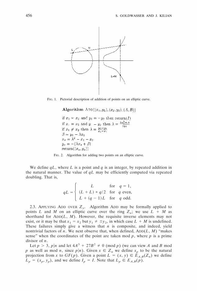
For elliptic curves over the reals, we can interpret our addition operation asillustrated in Figure 1 (this is known as the “tangent and chord” method). Forthe “general case”, given points L and M, we first consider the line connecting Land M, and locate the third intersection point of the line with the points on curve( A, B). We then reflect this third point over the x-axis, and define the resultingpoint as L 1 M.

Some degenerate cases remain. If L 5 M, instead use the line tangent to theelliptic curve at L. If L and M are on a vertical line, we define L 1 M 5 I.Finally, if the line L and M fails to intersect the curve any other point, it can beshown that the line will be tangent to the curve at one of the two points ofintersection. We treat this tangency as a double point of intersection, and use itas the “third” point.

Expressing these geometric operations algebraically, the resulting algorithm isgiven in Figure 2. This algorithm works for arbitrary fields such that 2, 3 Þ 0.


We define qL, where L is a point and q is an integer, by repeated addition inthe natural manner. The value of qL may be efficiently computed via repeateddoubling. That is,

qL 5 5 L for q 5 1,~L 1 L! p q/ 2 for q even,L 1 ~q 2 1! L for q odd.

2.3. APPLYING ADD OVER ZN. Algorithm ADD may be formally applied topoints L and M on an elliptic curve over the ring Zn; we use L 1 M asshorthand for ADD(L, M). However, the requisite inverse elements may notexist, or it may be that x1 5 x2 but y1 Þ 6y2, in which case L 1 M is undefined.These failures simply give a witness that n is composite, and indeed, yieldnontrivial factors of n. We next observe that, when defined, ADD(L, M) “makessense” when the coordinates of the point are taken mod p, where p is a primedivisor of n.

Let p . 3, p un and let 4A3 1 27B2 Þ 0 (mod p) (we can view A and B modp as well as mod n, since p un). Given x [ Zn we define xp to be the naturalprojection from x to GF( p). Given a point L 5 ( x, y) [ EA, B(Zn) we defineLp 5 ( xp, yp), and we define Ip 5 I. Note that Lp [ EA, B( p).

FIG. 1. Pictorial description of addition of points on an elliptic curve.

FIG. 2. Algorithm for adding two points on an elliptic curve.


LEMMA 1. If L 1 M is defined, then (L 1 M)p 5 Lp 1 Mp.

PROOF. The lemma trivially holds if L or M is the identity; for the rest of theproof we write L 5 ( x1, y1) and M 5 ( x2, y2). First, note that for any rationalfunction R over Zn, either R( x1, x2, . . .) is undefined or

~R~ x1 , x2 , · · ·!p!p 5 R~~ x1!p , ~ x2!p , · · ·! ,

Where in computing R(( x1)p, ( x2)p, . . .) the coefficients of R are taken mod pinstead of mod n.

Algorithm ADD considers 3 cases:

(1) x1 5 x2 and y1 5 2y2, in which case ADD returns I.(2) x1 5 x2 and y1 5 y2, in which case ADD returns

SP~ x1 , x2 , y1 , y2 , A, B!

~2y1!3

,Q~ x1 , x2 , y1 , y2 , A, B!

~2y1!3 D .

(3) x1 Þ x2, in which case ADD returns

SR~ x1 , x2 , y1 , y2 , A, B!

~ x2 2 x1!3

,S~ x1 , x2 , y1 , y2 , A, B!

~ x2 2 x1!3 D .

Here, P, Q, R, and S are polynomials. If (L, M) and (Lp, Mp) both fall into thesame case, then ADD will compute the same rational function on x1, x2, y1, y2 asit computes on ( x1)p, ( x2)p, ( y1)p, ( y2)p, and the lemma follows. It remains toshow that whenever (L, M) and (Lp, Mp) fall into different cases, L 1 M isundefined. This event can happen if either

(1) x1 5 x2, but y1 Þ 6y2 or(2) x1 Þ x2, but ( x1)p 5 ( x2)p

(The other “possibilities” can be eliminated since a 5 b implies ap 5 bp anda 5 2b implies ap 5 2bp.) In the former case, ADD is undefined. In the lattercase, p u( x1 2 x2), and ADD will thus be unable to compute the inverse of x1 2x2. e

2.4. THE GROUP STRUCTURE OF CURVES OVER GF( P). We use some classicalresults about curves over Zp, as well as some more recent results. First, the set ofpoints of the elliptic curve ( A, B) over Zp form an Abelian group under thepoint addition operation defined above. This group is isomorphic to Zm1

1 3 Zm2

1

for some m1, m2, where m1um2 and Zmi

1 denotes the cyclic additive group ofintegers mod mi.

We next consider the size of these groups. Given an elliptic curve ( A, B), wedenote by #p( A, B) the number of points on ( A, B) over GF( p). For the restof our discussion, we assume that p Þ 2, 3. The well-known Riemann Hypothesisfor Finite Fields implies that

p 1 1 2 2 Îp # #p~ A, B! # p 1 1 1 2 Îp .

The following theorem of Lenstra [1987] considers the distribution of #p( A, B)when ( A, B) is uniformly distributed. This result is crucial to our analysis.


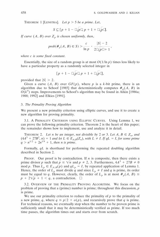
THEOREM 1 [LENSTRA]. Let p . 5 be a prime. Let,

S # @ p 1 1 2 Îp , p 1 1 1 Îp# .

If curve ( A, B) over Zp is chosen uniformly, then,

prob~#p~ A, B! [ S! .c

ln pz

uS u 2 2

2 Îp 1 1,

where c is some fixed constant.

Essentially, the size of a random group is at most O(1/ln p) times less likely tohave a particular property as a randomly selected integer in

@ p 1 1 2 Îp , p 1 1 1 Îp# ,

provided that uS u . 2.Given a curve ( A, B) over GF( p), where p is a k-bit prime, there is an

algorithm due to Schoof [1985] that deterministically computes #p( A, B) inO(k9) steps. Improvements to Schoof’s algorithm may be found in Atkin [1986a;1988; 1992] and Elkies [1991].

3. The Primality Proving Algorithm

We present a new primality criterion using elliptic curves, and use it to create anew algorithm for proving primality.

3.1. A PRIMALITY CRITERION USING ELLIPTIC CURVES. Using Lemma 1, wecan prove the following primality criterion. Theorem 2 is the heart of this paper;the remainder shows how to implement, use and analyze it in detail.

THEOREM 2. Let n be an integer, not divisible by 2 or 3. Let A, B [ Zn, and(4A3 1 27B2, n) 5 1 and let L [ EA,B(Zn), with L Þ I. If qL 5 I, for some primeq . n1/2 1 2n1/4 1 1, then n is prime.

Formally, qL is shorthand for performing the repeated doubling algorithmdescribed in Section 2.

PROOF. Our proof is by contradiction. If n is composite, then there exists aprime divisor p such that p # =n and p Þ 2, 3. Furthermore, 4A3 1 27B Þ 0mod p. Thus Lp [ EA, B( p) and qLp 5 I, by repeated application of Lemma 1.Hence, the order of Lp must divide q and since Lp Þ I and q is prime, its ordermust be equal to q. However, clearly, the order of Lp is at most #p( A, B) #p 1 2=p 1 1 , q, a contradiction. e

3.2. OVERVIEW OF THE PRIMALITY PROVING ALGORITHM. We focus on theproblem of proving that a (prime) number is prime; throughout this discussion, pis prime.

We use our primality criterion to reduce the primality of p to the primality ofa new prime, q, where q # p/ 2 1 o( p), and recursively prove that q is prime.For technical reasons, we eventually stop when the number to be proven prime issufficiently small that it may be deterministically verified as prime. If too muchtime passes, the algorithm times out and starts over from scratch.


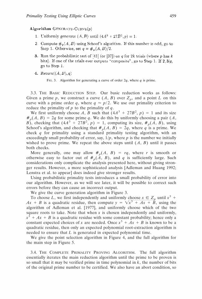
3.3. THE BASIC REDUCTION STEP. Our basic reduction works as follows:Given a prime p, we construct a curve ( A, B) over Zp, and a point L on thiscurve with a prime order q, where q ' p/ 2. We use our primality criterion toreduce the primality of p to the primality of q.

We first uniformly choose A, B such that (4A3 1 27B2, p) 5 1 and its size#p( A, B) 5 2q for some prime q. We do this by uniformly choosing a pair ( A,B), checking that (4A3 1 27B2, p) 5 1, computing its size, #p( A, B), usingSchoof’s algorithm, and checking that #p( A, B) 5 2q, where q is a prime. Wecheck q for primality using a standard primality testing algorithm, with anexceedingly small probability of error, say, 1/p, where p is the number we initiallywished to prove prime. We repeat the above steps until ( A, B) until it passesboth checks.

More generally, one may allow #p( A, B) 5 rq, where r is smooth orotherwise easy to factor out of #p( A, B), and q is sufficiently large. Suchconsiderations only complicate the analysis presented here, without giving stron-ger results. However, a more sophisticated analysis [Adleman and Huang 1992;Lenstra et al. to appear] does indeed give stronger results.

Using probabilistic primality tests introduces a small probability of error intoour algorithm. However, as we will see later, it will be possible to correct sucherrors before they can cause an incorrect output.

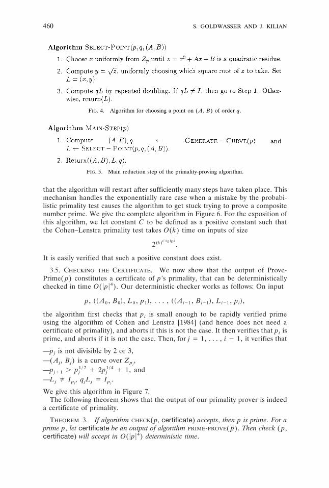
We give the curve generation algorithm in Figure 3.To choose L, we first independently and uniformly choose x [ Zp until x3 1

Ax 1 B is a quadratic residue, then compute y 5 =x3 1 Ax 1 B, using thealgorithm of Adleman et al. [1977], and uniformly choose which of the twosquare roots to take. Note that when x is chosen independently and uniformly,x3 1 Ax 1 B is a quadratic residue with some constant probability; hence only aconstant expected choices of x are needed. Once x3 1 Ax 1 B is known to be aquadratic residue, then only an expected polynomial root-extraction algorithm isneeded to ensure that L is generated in expected polynomial time.

We give the point selection algorithm in Figure 4, and the full algorithm forthe main step in Figure 5.

3.4. THE COMPLETE PRIMALITY PROVING ALGORITHM. The full algorithmessentially iterates the main reduction algorithm until the prime to be proven isso small that it may be verified prime in time polynomial in k, the number of bitsof the original prime number to be certified. We also have an abort condition, so

FIG. 3. Algorithm for generating a curve of order 2q, where q is prime.


that the algorithm will restart after sufficiently many steps have taken place. Thismechanism handles the exponentially rare case when a mistake by the probabi-listic primality test causes the algorithm to get stuck trying to prove a compositenumber prime. We give the complete algorithm in Figure 6. For the exposition ofthis algorithm, we let constant C to be defined as a positive constant such thatthe Cohen–Lenstra primality test takes O(k) time on inputs of size

2(k)C/lg lg k

.

It is easily verified that such a positive constant does exist.

3.5. CHECKING THE CERTIFICATE. We now show that the output of Prove-Prime( p) constitutes a certificate of p’s primality, that can be deterministicallychecked in time O( up u4). Our deterministic checker works as follows: On input

p, ~~ A0 , B0! , L0 , p1! , . . . , ~~ Ai21 , Bi21! , Li21 , pi! ,

the algorithm first checks that pi is small enough to be rapidly verified primeusing the algorithm of Cohen and Lenstra [1984] (and hence does not need acertificate of primality), and aborts if this is not the case. It then verifies that pi isprime, and aborts if it is not the case. Then, for j 5 1, . . . , i 2 1, it verifies that

—pj is not divisible by 2 or 3,—( Aj, Bj) is a curve over Zpj

,—pj11 . pj

1/ 2 1 2pj1/4 1 1, and

—Lj Þ Ipj, qjLj 5 Ipj

.

We give this algorithm in Figure 7.The following theorem shows that the output of our primality prover is indeed

a certificate of primality.

THEOREM 3. If algorithm CHECK( p, certificate) accepts, then p is prime. For aprime p, let certificate be an output of algorithm PRIME-PROVE( p). Then check ( p,certificate) will accept in O( up u4) deterministic time.

FIG. 4. Algorithm for choosing a point on ( A, B) of order q.

FIG. 5. Main reduction step of the primality-proving algorithm.


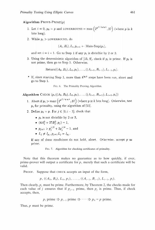
Note that this theorem makes no guarantee as to how quickly, if ever,prime-prover will output a certificate for p, merely that such a certificate will bevalid.

PROOF. Suppose that CHECK accepts an input of the form,

p, ~~ A0 , B0! , L0 , p1! , . . . , ~~ Ai21 , Bi21! , Li21 , pi! .

Then clearly, pi must be prime. Furthermore, by Theorem 2, the checks made foreach value of j ensures that if pj11 prime, then pj is prime. Thus, if checkaccepts, then,

pi prime f pi21 prime f · · · f p0 5 p prime.

Thus, p must be prime.

FIG. 6. The Primality Proving Algorithm.

FIG. 7. Algorithm for checking certificates of primality.


We now show that CHECK will always accept a certificate, of the above form,presented to it by PROVE-PRIME. We first note that by the definition of PROVE-PRIME, pi will be prime. By the definition of GENERATE-CURVE, we have (4Aj

3 127Bj

2, pj) 5 1. From the definition of GENERATE-CURVE, and the fact that#pj

( Aj, Bj) $ pj 1 1 2 2=pj, we have

pj11 $pj 1 1 2 2 Îpj

2

. pj1/ 2 1 2pj

1/4 1 1,

for pj . 37. By the definition of PROVE-PRIME, pj . 37, unless p # 37, in whichcase it is easily verified that the output of PROVE-PRIME will be accepted byCHECK. Finally, by the definition of SELECT-POINT, Lj Þ Ipj

, and pj11Lj 5 Ipj.

Therefore, check will accept.To compute how many steps are required for a k-bit prime, we first note that

pj11 5 pj/ 2 1 o( pj), and therefore i 5 O(lg p) 5 O(k). For each value of jthe checking procedure must perform a constant number of simple arithmeticoperations, a single GCD computation, and must multiply a point Lj by aninteger qj. This all can be done in O(k3), so the total running time of thechecking algorithm is O(k3) z O(k) 5 O(k4) steps.

4. Analyzing the Main Step

We now analyze the running time of MAIN-STEP in terms of the number ofprimes in an appropriate interval around p/ 2. Define S( p) by

S~ p! 5 H q:q [ F p 1 1 2 Îp

2,

p 1 1 1 Îp

2 G , q prime.J .

LEMMA 2. Let p . 5 be a k-bit prime, and suppose that uS( p)u 5 O(=p/lgc p).Then algorithm MAIN-STEP( p) will run for expected O(kc18) steps before it termi-nates.

PROOF. We bound the time required by GENERATE-CURVE; the SELECT-POINT

procedure takes comparatively little time. Our procedure for finding a curve ( A,B) of order 2q will take expected time equal to the expected time necessary togenerate and test a single curve, multiplied by the expected number of curves itmust try. The time necessary to test a curve is dominated by Schoof’s algorithmwhich takes O( up u8) steps. The expected time necessary to generate a curve,compute (4A3 1 27B2, p) and to run the probabilistic primality tests are lowerorder polynomials in up u.

We now bound the expected number of curves ( A, B) we must try. For primep, and for any value of A, there are at most two bad values of B, 6=24A3/ 27mod p. Thus, with overwhelming probability, a randomly chosen ( A, B) willconstitute an elliptic curve. To bound the number of curves we must test beforecoming up with one whose order is twice a prime, we use Lenstra’s theorem torelate this number to the size of the set S( p).


LEMMA 3. Let p . 5 be a prime, and let ( A, B) be chosen uniformly fromcurves over Zp. Let S( p) be defined as above. Then

prob~#p~ A, B! is twice a prime! .c

lg pz

uS~ p! u 2 2

2 Îp 1 1,

where c is some fixed constant.

PROOF. There is a trivial bijection between numbers in the interval

@ p 1 1 2 Îp , p 1 1 1 Îp#

which are twice a prime, and elements of S( p). Applying Lenstra’s theoremimmediately gives the desired bound. e

By taking the reciprocal of this bound on the probability, and a simplecalculation, we have that GENERATE-CURVE takes only O(kc19) expected steps.

It remains to verify that SELECT-POINT requires much less than O(kc19)expected steps. Assume that EA, B( p) is of order 2q, where q is a prime. Recallthat group EA, B( p) is isomorphic to a product of cyclic additive groups, Zm1

3Zm1

, where m1um2. Since EA, B( p) is of size 2q, we have m1m2 5 2q, and hencem1 5 1, m2 5 2q, for q . 2. Thus, EA, B( p) will in fact be isomorphic to Z2q.Since Z2q has q 2 1 points of order q, so must EA, B( p). Now, note that thesepoints are paired: since ( x, y) and ( x, 2y) are inverse, q( x, y) 5 I iff q( x,2y) 5 I. Thus, there are at least (q 2 1)/ 2 values of x such that choosing x andy 5 =x3 1 Ax 1 B will give a point on the curve of order q. Thus, the expectedrunning time of SELECT-POINT is 2p/(q 2 1) 5 O(1) times the amount of timeit takes to randomly choose x, compute y 5 =x3 1 Ax 1 B, and check that q( x,y) 5 I. Checking that z 5 x3 1 Ax 1 B is a quadratic residue, and thencomputing a square root of z using the algorithm of Adleman et al. [1977] naivelytakes O( up u4) time. Note that the algorithm of [8] requires a quadratic nonresi-due. One can simply choose an element of GF( p) at random until one finds one,with a 1/2 probability of success each time; this step is a lower order contributionto the overall running time. Similarly, it takes O(k3) steps to add two points andO(lg q) 5 O(k) steps to check that qL 5 I using repeated doubling. Thus, atmost O(k4) expected steps are naively required. These naive running times canbe improved, but suffices to show that the time required by SELECT-POINT is alow-order term. e

5. Analysis of the Primality Proving Algorithm

In the previous section, we exhibited our primality proving algorithm, anddemonstrated that it produced legitimate certificates of primality. We also gavethe running-time analysis of the main step of the algorithm, as a function of thenumber of primes in certain intervals.

In this section, we analyze how long it takes for the entire algorithm toproduce proofs of primality. We show that, modulo a conjecture on the distribu-tion of prime numbers, the algorithm will always halt in expected polynomialtime. We then extend this argument to show that the algorithm will produce


proofs of primality, in expected polynomial time, for all but a vanishing fractionof the prime numbers. This latter theorem does not depend on any conjectures.

5.1. ANALYSIS BASED ON A CONJECTURE. Using the machinery of the previoussections, it is straightforward to analyze the running time of our algorithm underan assumption about the distribution of primes. In the next section, we considera relaxed, provable version of this assumption, under which we can show that ouralgorithm runs fast on most prime inputs.

THEOREM 4. Suppose that,

~?c1 , c2 . 0!p~ x 1 Îx! 2 p~ x! $c2 Îx

logc1 x.

then algorithm PROVE-PRIME( p) will terminate in expected time O( up uc119) for psufficiently large.

PROOF. For ease of exposition, we assume that the probabilistic primalitytester used subroutine never incorrectly identifies a composite number as prime,and that the time-out feature is never invoked. We then observe that droppingthese assumptions doesn’t significantly affect the analysis.

Let us simplify the expression for S( pj). Setting x 5 ( pj 1 1 2 =pj)/ 2,and y 5 ( pj 1 1 1 =pj)/ 2, we have,

S~ pj! 5 $q [ @ x, y# , q prime% .

For pj . 37, y . x 1 =x, and thus there must be V(=x/logc1 x) primes inS( pj). Therefore, by Corollary 2, GENERATE-CURVE( pj) will take expectedO( upju

c118) # O(kc118) steps (where upju denotes the number of bits of pj).Thus, the algorithm will, in this optimistic scenario, run in expected O(kc119)time.

We now account for the possibility of a bad event: the algorithm timing-out ornot detecting a composite. In each case, we assume that the algorithm runs forthe maximum number of steps, denoted M, and then restarts. Let r denote theprobability of a bad event, and E denote the expected number of steps thealgorithm takes conditioned on no bad event occurring. Then by a straightfor-ward analysis, the total expected time of the algorithm will be bounded above by

~r 1 r2 1 · · ·! M 1 E # O~rM 1 E! ,

when r # 1/2. Now, M is bounded by k lg k by design and from the above analysis,E 5 O(kc119). It remains to bound r. The algorithm will never make more thanM calls to the primality test, and the failure rate on any individual test is at most1/LOWERBOUND, so the total probability of a primality test failing is M z 22kC/lg lg k

,which is insignificant (,, 1/M2, for large p). If the algorithm doesn’t make amistake in its primality test, then by Markoff’s inequality, the algorithm will takemore than M steps with probability at most E/M. Hence, the algorithm will runfor at most O((E/M 1 o(1/M2)) M 1 E) 5 O(E) expected steps. Indeed, thisanalysis is quite weak; the increase in the expected time from these effects ismuch smaller. Also, note that if for small p a more reasonable choice of time-out


limits and error thresholds for the ordinary probabilistic primality tests weremade, then this analysis would work for all p. e

5.2. PROVING OUR ALGORITHM FAST FOR MOST PRIMES. The scenario in theprevious section is optimistic. It assumes that whenever one is attempting toshow a number p prime, there will always be sufficiently many primes in theinterval

F p 1 1 2 Îp

2,

p 1 1 1 Îp

2 G .

That is, S( p) is assumed to be sufficiently large. This is almost certainly the casefor all primes, but it is currently beyond our ability to prove this fact. However, ithas been shown that intervals that contain a sparse number of primes are rare.We have the following result, which is implied by a technical lemma ofHeath-Brown [1978] (communicated to us by H. Maier and C. Pomerance).

THEOREM 5 [HEATH-BROWN]. Call an integer y sparse if there are less than=y/2ln y primes in the interval [ y, y 1 =y]. Then there exist a constant a suchthat for sufficiently large x,

u$ y:y [ @ x, 2x# , y is sparse% u , x5/6lnax.

We use this result to show that our algorithm is fast for most prime numbers.Let BAD(k, T) denote the set of k-bit primes p such that PROVE-PRIME fails tooutput a certificate of primality for p in expected T steps. We prove the followingtheorem:

THEOREM 6. There exist c1, c2 . 0 such that for k sufficiently large,

BAD~k, c1k11! #2k

2kc2/lg lg k

PROOF. Given a prime p, we denote by Pi( p) the set of all intermediateprimes that can be generated in step i of the algorithm. In other words, Pi( p)consists of all primes that could conceivably be equal to pi in the certificategenerated for p. Thus, for instance,

P0~ p! 5 $ p% , P1~ p! # F p 1 1 2 2 Îp

2,

p 1 1 1 2 Îp

2 G , . . .

These are the only primes that need be considered for proving p prime. If it isthe case that S( pi) is O(=pi/ln pi) for pi [ Pi( p), then by the same analysis asin the proof of Theorem 4, PROVE-PRIME( p) will terminate in expected timeO(k11). The rest of this proof consists of showing that this will be true for mostprimes.

Our proof proceeds in three stages. First, we bound the range in which Pi( p)falls, and use this bound to derive a simple criterion which implies that S( pi) islarge for pi [ Pi( p). Next, we use a result of Heath-Brown, and a simplecombinatoric argument, to show that our criterion will fail for only a relatively


small number of values of Pi( p). Finally, we use this result to bound the numberof primes for which our algorithm is slow.

5.2.1. Characterizing Pi( p). We note that for every certificate, pi11 5 pi/ 2 1o( pi). This would suggest Pi( p) should be clustered around p/ 2 i, as follows:

LEMMA 4. Let p be a prime, and let p/2i be sufficiently large. Then any elementof Pi( p) lies in the range,

S p

2 i2 7 Îp

2 i,

p

2 i1 7 Îp

2 iD .

Remark. The value of 7 that we obtain can be improved on. However, we onlyneed to establish that some constant exists.

PROOF. Our proof is by induction on i. For i 5 0, the lemma clearly holds.We can bound the largest and smallest elements of Pi( p) in terms of the largestand smallest elements of Pi21( p). Specifically, we have

max~Pi~ p!! #max~Pi21~ p!! 1 1 1 2 Îmax~Pi21~ p!!

2, and,

min~Pi~ p!! $min~Pi21~ p!! 1 1 2 2 Îmin~Pi21~ p!!

2.

By inductive hypothesis, we have,

max~Pi~ p!! #p/ 2 i21 1 7 Îp/ 2 i21 1 1 1 2 Îp/ 2 i21 1 7 Îp/ 2 i21

2.

We can simplify the above expression considerably. We note that,

x 1 7 Îx , ~1 1 o~1!! x,

for x sufficiently large,

p/ 2 i21

25

p

2 i,

and,

Î p

2 i215 Î2 z Îp

2 i.


These simplifications yield,

max~Pi~ p!! ,p

2 i1 S 7

Î21 Î2 1 o~1!D Îp

2 i1 1

,p

2 i1 7 Îp

2 i,

For p/ 2 i sufficiently large. The lower bound is similarly established. e

5.2.2. A Condition under which S( pi) Will be Large. We can use Lemma 4 togive a simple condition under which we can guarantee that S( pi) will be large forall pi [ Pi( p). To facilitate the discussion, we first define a parameterized familyof intervals, ( i( p).

Definition 3. Let ( i( p) denote the set of intervals of the form

F pi 1 1 2 Îpi

2,

pi 1 1 1 Îpi

2 G ,

where pi [ Pi( p).

That is, ( i( p) is the set of intervals which are important in our primalityproving algorithm’s search for pi11. If we can show that every interval in ( i( p)has a large number of primes, then we are guaranteed that our algorithm willalways be able to quickly generate pi11.

Note that the above definition uses a =p instead of a 2=p that one mightexpect given the Riemann hypothesis for finite fields. This is due to ourdefinition of 6( pi), and more fundamentally due to the fact that Lenstra’s resultonly holds for the smaller interval.

To bound the number of primes in each interval in ( i( p), we consider aconstant-sized set of intervals, # i( p), as follows.

Definition 4. Let # i( p) be defined as the set of intervals,

H @ xj , xj 1 Îxj#: xj 5 p

2 i111

j

3z Î p

2 i11 , j [ @222, 22#J .

(The value of 22 can probably be reduced, but we only need the fact that someconstant exists.)

LEMMA 5. Let p be a prime, and let p/2i be sufficiently large. Then every intervalin (i( p) contains an interval in #i( p).

Thus, if every interval in # i( p) has enough primes then every interval in ( i( p)has enough primes.

PROOF. Let [ x, y] [ ( i( p). We have,

y 5 x 1 ~ Î2 1 o~1!! Îx .


By the same argument as in Lemma 4, we have,

p

2 i111 7 Î p

2 i11$ x $

p

2 i112 7 Î p

2 i11.

Thus, for some j [ [221, 21], xj21 # x # xj, where xj is as in Definition 4. Weclaim that [ x, y] contains the interval [ xj, xj 1 =xj] [ # i( p); we must showthat y $ xj 1 =xj.

First, it is easily verified that x, xj 5 (1 1 o(1)) p/ 2 i11 (where the o(1) termgoes to 0 as p/2i grows sufficiently large). Next, xj 2 x # xj 2 xj21 5 =p/2i11/3 1O(1) (the O(1) compensates for the rounding. Hence, (xj 1 =xj) 2 x 5 (4/3 1o(1))=p/2i11. However, y 2 x 5 (=2 1 o(1))=p/2i11, hence y $ x for p/2i

sufficiently large. e

5.2.3. A Further Property of #i( p). Lemma 5 is crucial to our analysis. Insteadof having to show that u( i( p) u 5 O(=p/ 2 i11) intervals all have sufficientlymany primes, we need only show that,

u# i~ p! u 5 O~1! ,

intervals have sufficiently many primes (for most primes p). We first extend ournotion of sparseness to # i( p).

Definition 5. Let p be a prime. We say that # i( p) is sparse if any of theintervals in # i( p) is sparse.

Heath-Brown shows that only a vanishing fraction of the intervals of the form[ x, x 1 =x] will not have enough primes. But if these “bad” intervals appearin most sets # i( p) they could destroy a disproportionate number of primes. Thefollowing lemma bounds this effect:

LEMMA 6. Let x be sufficiently large. Then an interval of the form,

@ x, x 1 Îx# ,

can be in # i( p) for at most c z 2 i different values of p , where c is some constant.

PROOF. It suffices to show that there are, for each value of k [ [222, 22],only O(2 i) values of p which satisfy the equation fk( p) 5 x, where,

fk~ p! 5p

2 i111

k

3z Î p

2 i11.

We first eliminate the integer rounding by noting that

z 5 x f x 2 1 # z # x 1 1.

We therefore have to show that there are only O(2 i) integers p which satisfy,

x 2 1 # fk~ p! # x 1 1.

Therefore, if [ x, x 1 =x] is in # i( p) and # i( p9), then ufk( p9) 2 fk( p) u # 2.We will use this fact to show that p and p9 must be near to each other in value,


which will in turn give us the desired bound. For the rest of the proof, we assumewithout loss of generality that p # p9.

Let us consider fk in the continuous domain. For all p . 0, the derivativef9k( p) is at least 22(i11). Since fk is clearly monotone increasing, we havefk( p9) 2 fk( p) # 2. By elementary calculus, we have,

fk~ p9! 2 fk~ p! $p9 2 p

2 i11,

from which we can derive,

p9 2 p # 2 z 2 i11.

This clearly implies that only c z 2 i solutions exist, for some constant c. e

5.2.4. The Final Calculation. We now bound the number of primes for whichour algorithm will fail. First, we argue that the number of k-bit primes p suchthat # i( p) will be sparse will be small, where c is a positive constant.

LEMMA 7. Let 2k2i be sufficiently large. At most, 2k/2(1/7)(k2i) k-bit primes p aresuch that #i( p) is sparse.

Remark. Here, 1/7 may be replaced by any number less than 1/6.

PROOF. First, we note that if [ x, x 1 =x] is in # i( p) for p [ [2k21, 2k],then x [ [2k2i22, 2k2i11]. This follows from the definition of # i( p) and thebounds on p. We now use Heath-Brown’s theorem on the intervals [2k2i22,2k2i21], [2k2i21, 2k2i], and [2k2i, 2k2i11], and sum the results. This boundsthe number of sparse intervals in

ø

p[[2k21, 2k]

# i~ p! ,

to at most,

Oj50

2

2(5/6)(k2i2j) loga2k2i2j # c1 z 2(5/6)(k2i)loga2k2i,

for some constant c1. By Lemma 6, each sparse interval of this form is in # i( p)for at most c22 i different values of p, where c2 is some constant. Thus, at most

~c2 z 2 i!~c1 z 2(5/6)(k2i)loga2k2i! 5 c1c2

2kloga2k2i

2(1/6)(k2i)

#2k

2(1/7)(k2i),

for 2k2i sufficiently large. e

We now upper-bound the number of k-bit primes that PROVE-PRIME will notquickly certify as prime. In order for a prime p to not be quickly certified, as per


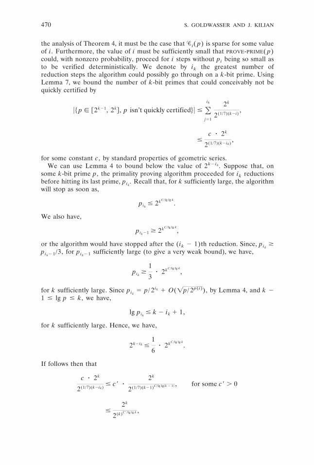
the analysis of Theorem 4, it must be the case that # i( p) is sparse for some valueof i. Furthermore, the value of i must be sufficiently small that PROVE-PRIME( p)could, with nonzero probability, proceed for i steps without pi being so small asto be verified deterministically. We denote by ik the greatest number ofreduction steps the algorithm could possibly go through on a k-bit prime. UsingLemma 7, we bound the number of k-bit primes that could conceivably not bequickly certified by

u$ p [ @2k21, 2k# , p isn’t quickly certified% u # Oj51

ik 2k

2(1/7)(k2i),

#c z 2k

2(1/7)(k2ik),

for some constant c, by standard properties of geometric series.We can use Lemma 4 to bound below the value of 2k2ik. Suppose that, on

some k-bit prime p, the primality proving algorithm proceeded for ik reductionsbefore hitting its last prime, pik

. Recall that, for k sufficiently large, the algorithmwill stop as soon as,

pik# 2kC/lg lg k

.

We also have,

pik21 $ 2kC/lg lg k

,

or the algorithm would have stopped after the (ik 2 1)th reduction. Since, pik$

pik21/3, for pik21 sufficiently large (to give a very weak bound), we have,

pik$

1

3z 2kC/lg lg k

,

for k sufficiently large. Since pik5 p/ 2 ik 1 O(=p/ 2p(i)), by Lemma 4, and k 2

1 # lg p # k, we have,

lg pik# k 2 ik 1 1,

for k sufficiently large. Hence, we have,

2k2ik #1

6z 2kC/lg lg k

.

If follows then that

c z 2k

2(1/7)(k2ik)# c9 z

2k

2(1/7)(k21)C/lg lg~k 2 1! , for some c9 . 0

#2k

2(k)C9/lg lg k ,


for some suitably chosen C9. e

REFERENCES

ADLEMAN, L. M., AND HUANG, M. 1987. Recognizing primes in polynomial time. In Proceedings ofthe 19th Annual ACM Symposium on Theory of Computing (New York, N.Y., May 25–27). ACM,New York, pp. 462– 471.

ADLEMAN, L. M., AND HUANG, M. 1992. Primality testing and Abelian varieties over finite fields.In Lecture Notes in Mathematics, vol. 1512. Springer-Verlag, New York.

ADLEMAN, L. M., MANDERS, K., AND MILLER, G. L. 1977. On taking roots in finite fields. InProceedings of the 18th Annual Symposium on Foundations of Computer Science. IEEE, New York,pp. 175–178.

ADLEMAN, L. M., POMERANCE, C., AND RUMELY, R. 1983. On distinguishing prime numbers fromcomposite numbers. Ann. Math. 117, 173–206.

ATKIN, A. O. L. 1986a. Schoof’s algorithm. Manuscript.ATKIN, A. O. L. 1986b. Manuscript.ATKIN, A. O. L. 1988. The number of points on an elliptic curve modulo a prime. Manuscript.ATKIN, A. O. L. 1992. The number of points on an elliptic curve modulo a prime (II). Manuscript.ATKIN, A. O. L., AND MORAIN, F. 1993. Elliptic curves and primality proving. Math. Comput. 61,

203 (July), 29 – 68.BOSMA, W. 1985. Primality testing using elliptic curves. Tech. Rep. 8512. Math. Instituut, Univ.

Amsterdam, Amsterdam, The Netherlands.BOSMA, W., AND VAN DER HULST, M. P. 1990. Faster primality testing. In Proceedings of EUROC-

RYPT ’89. Lecture Notes in Computer Science, vol. 434. Springer-Verlag, New York, pp. 652– 656.BRILLHART, J., LEHMER, D. H., AND SELFRIDGE, J. L. 1975. New primality criteria and factoriza-

tions of 2m 6 1. Math. Comput. 29, 130, 620 – 647.BRILLHART, J., LEHMER, D. H., SELFRIDGE, J. L., TUCKERMAN, B., AND WAGSTAFF, JR., S. S. 1988.

Factorizations of bn 1 1; b 5 2, 3, 5, 6, 7, 10, 11, 12 up to high powers. Cont. Math. 2, 22.CHUDNOVSKY, D., AND CHUDNOVSKY, G. 1986. Sequences of numbers generated by addition in

formal groups and new primality and factorization tests. Adv. App. Math. 7.COHEN, H., AND LENSTRA, JR., H. W. 1984. Primality testing and Jacobi sums. Math. Comput. 42.ELKIES, N. D. 1991. Explicit isogenies. Manuscript.ELKIES, N. D. 1998. Elliptic and modular curves over finite fields and related computational

issues. In Computational Perspectives on Number Theory: Proceedings of a Conference in Honor ofA. O. L. Atkins, D. A. Buell and J. T. Teitelbaum, eds. AMS/IP Studies in Advanced Mathematics,vol. 7. American Mathematics Society, Providence, R. I., pp. 21–76.

GOLDWASSER, S., AND KILIAN, J. 1986. Almost all primes can be quickly certified. In Proceedings ofthe 18th Annual ACM Symposium on Theory of Computing (Berkeley, Calif., May 28 –30). ACM,New York, pp. 316 –329.

HEATH-BROWN, D. R. 1978. The differences between consecutive primes. J. London Math. Soc. 2,18, 7–13.

KALTOFEN, E., VALENTE, T., AND YUI, N. 1989. An improved Las Vegas primality test. InProceedings of the ACM-SIGSAM 1989 International Symposium on Symbolic and Algebraic Compu-tation (ISSAC ’89) (Portland, Ore., July 17–19), Gilt Gonnet, ed. ACM, New York, pp. 26 –33.

KILIAN, J. 1990. Uses of Randomness in Algorithms and Protocols. MIT Press, Cambridge, Mass.KONYAGIN, S., AND POMERANCE, C. 1997. On primes recognizable in deterministic polynomial

time. In The Mathematics of Paul Erdos, R. Graham and J. Nesetril, eds. Springer-Verlag, NewYork, pp. 177–198.

LENSTRA, JR., H. W. 1987. Factoring, integers with elliptic curves. Ann. Math. 126, 649 – 673.LENSTRA, A., AND LENSTRA, JR., H. W. 1987. Algorithms in number theory. Tech. Rep. 87-008.

Univ. Chicago, Chicago, Ill.LENSTRA, JR., H. W., PILA, J., AND POMERANCE, C. 1993. A hyperelliptic smoothness test, I. Philos.

Trans. Roy Soc. London Ser. A 345, 397– 408.LENSTRA, JR., H. W., PILA, J., AND POMERANCE, C. 1999. A hyperelliptic smoothness test, II.

Manuscript.LENSTRA, JR., H. W., PILA, J., AND POMERANCE, C. 1999. A hyperelliptic smoothness test, III. To

appear.


MIHAILESCU, P. 1994. Cyclotomy primality proving—Recent developments. In Proceedings of the3rd International Algorithmic Number Theory Symposium (ANTS). Lecture Notes in ComputerScience, vol. 877. Springer-Verlag, New York, pp. 95–110.

MILLER, G. L. 1976. Riemann’s hypothesis and test for primality. J. Comput. Syst. Sci. 13, 300 –317.MORAIN, F. 1990. Courbes elliptques et tests de primalite. Ph.D. dissertation. Univ. Claude

Bernard-Lyon I.MORAIN, F. 1995. Calcul de nombre de points sur une courbe elliptique dans un corps fini:

Aspects algorithmiques. J. Theor. Nombres Bordeaux 7, 255–282.PINTZ, J., STEIGER, W., AND SZEMEREDI, E. 1989. Infinite sets of primes with fast primality tests

and quick generation of large primes. Math. Comput. 53, 187, 399 – 406.POMERANCE, C. 1987. Very short primality proofs. Math. Comput. 48, 177, 315–322.PRATT, V. R. 1975. Every prime has a succinct certificate. SIAM J. Comput. 4, 3, 214 –220.RABIN, M. 1980. Probabilistic algorithms for testing primality. J. Numb. Theory 12, 128 –138.SCHOOF, R. 1985. Elliptic curves over finite fields and the computation of square roots modulo p.

Math. Comput. 44, 483– 494.SCHOOF, R. 1995. Counting points on elliptic curves over finite fields. J. Theor. Nombres. Bordeaux

7, 219 –254.SILVERMAN, J. 1986. The arithmetic of elliptic curves. In Graduate Texts in Mathematics, vol. 106.

Springer-Verlag, New York.SOLOVAY, R., AND STRASSEN, V. 1977. A fast Monte-Carlo test for primality. SIAM J. Comput. 6, 1,

84 – 85.TATE, J. 1974. The arithmetic of elliptic curves. Invent. Math. 23, 179 –206.WILLIAMS, H. C. 1978. Primality testing on a computer. Ars. Combinat. 5, 127–185.WUNDERLICH, M. C. 1983. A performance analysis of a simple prime-testing algorithm. Math.

Comput. 40, 162, 709 –714.

RECEIVED FEBRUARY 1991; REVISED MAY 1999; ACCEPTED JUNE 1999

Journal of the ACM, Vol. 46, No. 4, July 1999.


Primality Testing Using Elliptic Curves

Documents

Transcript of Primality Testing Using Elliptic Curves