Pricing American-Style Options by Monte Carlo

Simulation: Alternatives to Ordinary Least Squares

Stathis Tompaidis

Chunyu Yang ∗

∗Tompaidis is with the McCombs School of Business, University of Texas at Austin, Information,

Risk and Operations Management and Finance departments, Austin, TX 78712, Tel. 512-4715252,

Stathis.Tompaidis@mccombs.utexas.edu. Yang is with the McCombs School of Business, University

of Texas at Austin, Information, Risk and Operations Management department, Austin, TX 78712,

Tel. 512-4711679, Chunyu.Yang@phd.mccombs.utexas.edu. The authors would like to thank seminar

participants at the University of Texas at Austin, and the Workshop on Computational Finance at the

Newton Institute in Cambridge.

Pricing American-Style Options by Monte Carlo Simulation:

Alternatives to Ordinary Least Squares

ABSTRACT

We investigate the performance of the Ordinary Least Squares (OLS) regression

method in Monte Carlo simulation algorithms for pricing American options. We

compare OLS regression against several alternatives and find that OLS regression

underperforms methods that penalize the size of coefficient estimates. The degree

of underperformance of OLS regression is greater when the number of simulation

paths is small, when the number of functions in the approximation scheme is

large, when European option prices are included in the approximation scheme,

and when the number of exercise opportunities is large. Based on our findings,

instead of using OLS regression we recommend an alternative method based on a

modification of Matching Projection Pursuit.

Introduction

Determining the price of American and Bermudan options that depend on a large number

of underlying assets is a question of both theoretical and practical interest, and has

attracted significant attention in the literature. On the theoretical side, the interest

arises because the price of an American option is given by the value function of an

optimal stopping problem. Practical interest, on the other hand, is due to the many

applications of American options. For example, an application from the area of real

options is the estimation of the option value to build a plant and the determination

of the optimal time to build. When the option value depends on several underlying

stochastic processes, many pricing methodologies become inadequate. Methods that

make use of a grid, such as finite difference or finite element methods, or the use of

multidimensional lattices, fail due to the curse of dimensionality: computational time

increases exponentially with the number of underlying stochastic factors. The only

methods whose computational burden remains manageable as the number of underlying

stochastic factors increases are based on Monte Carlo simulation.

The apparent difficulty to reconcile Monte Carlo simulation with the dynamic pro-

gramming framework used to solve optimal stopping problems has been resolved in

several ways in the literature. In this paper we concentrate on the function approxima-

tion approach introduced by Carriere (1996), where the continuation value function at

each possible exercise date is estimated by minimizing squared errors through the use

of smooth splines and local regressions. The method was further developed by Tsitsiklis

and Van Roy (1999), Tsitsiklis and Van Roy (2001), and Longstaff and Schwartz (2001),

who approximate the continuation value function by its projection on the linear span of

a set of functions, with the objective of minimizing squared errors.1

1There are slight differences between the methods: Tsitsiklis and Van Roy (2001) use all the sim-ulated paths to estimate the continuation value, while Longstaff and Schwartz (2001) only use pathsthat are in-the-money. For further discussion, extensions, as well as links with other methods, seeGlasserman (2004).

1

In this paper we follow the specification presented in Longstaff and Schwartz (2001),

and investigate the impact of choosing to minimize squared errors, to the quality of

the approximation. While the objective of minimizing squared errors has the advantage

that it can be implemented efficiently using Ordinary Least Squares (OLS) regression,

it is subject to overfitting and misspecification of the functions used as regressors.2 As

the potential for problems is greater when the number of simulation paths is small,

we compare the performance of OLS regression against several alternatives in a set of

testcases for a varying number of simulation paths. The alternatives we examine are

quantile regression; Tikhonov regularization; Matching Projection Pursuit (MPP); a

modified version of Matching Projection Pursuit (MMPP); as well as Classification and

Regression Trees (CART), a non-parametric method. All the methods are chosen for

their perceived robustness regarding small datasets: quantile regression relies on the

estimation of the median rather than the mean, and is less susceptible to a few large

fluctuations; the objective of Tikhonov regularization, MPP and MMPP is to minimize

squared errors plus a penalty for the size of the coefficients of the linear combination of

the functions used to approximate the continuation value function; CART is designed

specifically to deal with small datasets.

While OLS regression is the estimation method that produces the estimates with

the smallest variance among unbiased estimation methods, our findings demonstrate

that in the context of valuing American options, OLS regression is often a poor choice

when the number of simulated paths is small. In addition to performing worse than

other methods, notably the MMPP method, the performance of OLS regression deteri-

orates as the number of functions used to approximate the continuation value function

increases. Including functions that are likely to be similar to the continuation value

function, such as the prices of European options, deteriorates the approximation quality

of OLS regression even more. The deterioration in both cases appears to be due to a

2Overfitting is a loosely defined term. In the context of our paper, we consider overfitting to be poorout-of-sample performance compared to in-sample performance.

2

multi-collinearity problem. We find that the quality of the approximation using OLS

regression deteriorates as the number of exercise opportunities increases, indicating that

bias introduced at an early stage in the backward induction framework propagates and

results in an approximate option price far from the true value. A potential explanation to

the underperformance of OLS regression is that the estimates computed using Tikhonov

regularization, MPP and MMPP have lower variance than the OLS estimates, although

they may be biased. The larger variance of OLS regression leads to a rapid deterioration

in the OLS estimates, as the results of one estimation are used in a recursive fashion to

compute the previous — in terms of exercise dates — estimate.

The rest of this paper is organized as follows: Section I describes the general valua-

tion algorithm and alternative methods to OLS regression. Section II presents the five

testcases that we use to evaluate the performance of the different methods. Section III

discusses the experimental design of our study and the measures we use to evaluate

performance. Section IV presents our computational results. Section V concludes the

paper.

I. Valuation Algorithm

A. General Valuation Framework

Pricing American-style options through Monte Carlo simulation involves the general

framework of dynamic programming and function approximation. We describe the Least

Squares Monte Carlo (LSM) algorithm below and in Figure 1. Further details can be

found in Longstaff and Schwartz (2001).

3

The algorithm involves the generation of paths for the values of the state variables

by Monte Carlo simulation.3 We use the following notation: S(i)t is the value of the

state variables at time t along path i; h is the option payoff; V is the option value; and

{ti}Ni=0 are the possible exercise times. The algorithm approximates the continuation

value of the option at each possible exercise time by a linear combination of a set of

basis functions {φj}Nbj=1.

4

LSM Algorithm

Step 1: generate M paths for the values of the state variables at all possible exercise

times

Step 2: at the terminal time tN , set the option value V equal to the payoff

V(S

(m)tN

, tN

)= h

(S

(m)tN

, tN

),m = 1, ..., M

Step 3: for the set of paths {il}Ll=1, for which the option is in-the-money; i.e., h(Sil

tN−1, tN−1) >

0, find coefficients a∗j(tN−1) to minimize the norm

∥∥∥∥∥∥∥∥∥∥∥∥

Nb∑j=1

aj (tN−1)

φj(S(i1)tN−1

)

φj(S(i2)tN−1

)...

φj(S(iL)tN−1

)

− e−r(tN−tN−1)

V (S(i1)tN

, tN)

V (S(i2)tN

, tN)...

V (S(iL)tN

, tN)

∥∥∥∥∥∥∥∥∥∥∥∥3The state variables include the prices of the assets, but may also include the values of other stochastic

processes, such as the interest rate, the volatility and the running maximum or minimum of the priceof an asset.

4We are abusing terminology by calling the set of functions {φj}Nb

j=1 a basis. Ideally the linear span of

the functions {φj}Nb

j=1 would include the continuation value. Unfortunately this can not be guaranteedin the general case.

4

Step 4: for each path update the value function at time tN−1

V(S

(m)tN−1

, tN−1

)=

h(S

(m)tN−1

, tN−1

), if h

(S

(m)tN−1

, tN−1

)≥ ∑Nb

j=1 a∗j (tN−1) φj

(S

(m)tN−1

)

e−r(tN−tN−1)V(S

(m)tN

, tN

), otherwise

Step 5: repeat Steps 3 and 4 for possible exercise times tN−2, tN−3, ..., until time t0.

The inputs of the LSM algorithms are the number of Monte Carlo paths M , the

basis functions {φj}Nbj=1, and the vector norm ‖ · ‖. Longstaff and Schwartz (2001)

use polynomials for the basis functions and the L2 vector norm, which leads to OLS

regression.

B. Convergence

The convergence properties of the LSM algorithm have been studied by Clement, Lam-

berton, and Protter (2002). There are two types of approximations in the algorithm.

• Type I: approximate the continuation value by its projection on the linear space of a

finite set of basis functions.

• Type II: use Monte Carlo simulations and OLS regression to estimate the coefficients

of the basis functions.

Clement, Lamberton, and Protter (2002) showed that under certain regularity con-

ditions on the continuation value, Type II approximation error decreases to zero as the

number of simulation paths goes to infinity, holding the number of basis functions fixed

(fixed Type I approximation error). In addition, if the Type II approximation is exact;

i.e., the coefficients of the projection can be calculated without random errors, then the

Type I approximation error diminishes as polynomials of the state variables of increas-

ing degree are added to the basis functions. As the degree of the polynomials tends

to infinity, Type I error tends to zero; i.e., the algorithm converges to the true price

5

as the number of simulation paths and basis functions tends to infinity. If the linear

span of the basis functions does not include the continuation value function; i.e., the

Type I approximation is not exact, then there will always be an error in the overall

approximation, irrespective of the number of simulation paths.

Glasserman and Yu (2004) study the convergence rate of the algorithm when the

number of basis functions and the number of paths increase simultaneously. They

demonstrate that in certain cases, in order to guarantee convergence, the number of

paths must grow exponentially with the number of polynomial basis functions when the

underlying state variable follows Brownian motion, or faster than exponential when the

underlying state variable follows geometric Brownian motion.

C. Ordinary Least Squares and Alternatives

Among possible choices for the norm used in the minimization in Step 3 of the LSM al-

gorithm, the L2 norm has the advantage of being easy to implement, as it corresponds to

OLS regression. In this section, we discuss the benefits and drawbacks of OLS regression

and describe alternative norms and algorithms.

C.1. Ordinary Least Squares Regression

Given observations {yi}Li=1 and a set of regressors {xi}Nb

i=1, OLS regression finds the

coefficients {ai}Nb

i=1 that minimize the sum of squared errors:

mina

[L∑

i=1

(yi − yi)2

]= min

a

L∑i=1

yi −

(Nb∑j=1

ajxj

)

i

2

where ( )i corresponds to the ith component of a vector. In the context of this paper, the

observed values correspond to discounted option values from the next possible exercise

6

time; i.e., yi = e−r(tj+1−tj)V (S(i)tj+1

, tj). The regressors correspond to the basis functions

{φi}Nbi=1.

OLS regression has important optimality properties. For example, among all linear,

unbiased estimators, OLS regression is guaranteed to produce estimates of the coeffi-

cients {ai}Nb

i=1 with the smallest variance (Gauss-Markov theorem, see Greene (2000)).

For the purpose of pricing American-style options, using OLS regression can guarantee

the convergence of the computed price to the true option price as the number of simula-

tion paths and the number of basis functions go to infinity. However, it is possible that

biased estimators may produce estimates of the coefficients with smaller variance. The

problem of large variance in the estimation of the coefficients is particularly severe when

the number of regressors is large compared to the number of observations, and when

the regressors are highly correlated. Large variance in the estimates manifests itself as

poor out-of-sample performance, and is often loosely described as overfitting. In our

context, the problem is potentially more severe, since OLS estimates for one exercise

date influence the option values for prior exercise dates in a recursive fashion.

C.2. Quantile Regression – Least Absolute Error Regression

Quantile regression is a statistical method that estimates conditional quantile functions.

Just as OLS regression estimates the conditional mean, quantile regression estimates the

conditional median, as well as the full range of other conditional quantile functions. In

this paper, we use the median (50% quantile) regression to approximate the continuation

value. This is equivalent to the Least Absolute Error regression where one minimizes

the sum of absolute errors; i.e.,

mina

[L∑

i=1

|yi − yi|]

= mina

L∑i=1

∣∣∣∣∣∣yi −

(Nb∑j=1

ajxj

)

i

∣∣∣∣∣∣

7

The advantage of quantile regression is that the estimation is less likely to be influenced

by outliers, producing smaller variation in the coefficient estimates compared to OLS

regression.

Quantile regression software is available in most modern statistical software packages.

In this paper we use the “quantreg” package in R. More details about quantile regression

and the “quantreg” package can be found in Koenker and Hallock (2001).

C.3. Tikhonov Regularization

Tikhonov regularization is a regularization method developed by Phillips (1962) and

Tikhonov (1963) to treat ill-posed problems with nearly linearly dependent predictors.

The method involves a trade-off between the “size” of the regularized solution and the

“quality” of the solution in terms of fitting the given data. Tikhonov regularization can

be formulated as:

mina

L∑i=1

yi −

(Nb∑j=1

ajxj

)

i

2

+ λ2

L∑i=1

(Nb∑j=1

Lij (aj − aj)

)2

where y is the vector of observed values, x is a matrix whose columns correspond

to the predictors, a is the vector of the coefficients of the predictors, λ is a regu-

larization parameter that determines the trade-off between the size of the solution

measured by∑L

i=1

(∑Nb

j=1 Lij (aj − aj))2

, and the quality of the solution measured by

∑Li=1

(yi −

(∑Nb

j=1 ajxj

)i

)2

. The vector a is a prior estimate of a.5 L is a weight matrix.

In this paper, we set a = 0 and L = I, the identity matrix.

The choice of the regularization parameter λ is crucial and also case dependent.

To determine the “best” λ, a graphical tool called L-curve is often used to quantify the

5Smart choices of a can be helpful in improving the results, but hard to find with low computationalcost. Notice that when λ = 0, or when a is equal to the OLS regression estimate, Tikhonov regularizationis equivalent to OLS regression. We have used Matching Projection Pursuit (described in the nextsection) to generate a, but did not see any improvement in the results.

8

trade-off between size and quality. A typical L-curve is shown in Figure 2. The “optimal”

regularization parameter λ∗ corresponds to the corner point in the figure. Choosing λ >

λ∗ tends to over-control the size and leads to poor quality of data fitting. On the other

hand, choosing λ < λ∗ leads to better fitting of the data, but with rapidly increasing

solution size, which is prone to overfitting. More information about the L-curve and its

applications can be found in Hansen (2001). We use the Regularization Tools package

in Matlab, developed by Hansen (1994), to perform Tikhonov regularization.

C.4. Matching Projection Pursuit

The projection pursuit method was developed by Kruskal (1969) to interpret high-

dimensional data with well-chosen lower-dimensional projections. The idea is to re-

cursively identify optimal projection directions with respect to minimizing residuals in

a hierarchical fashion, one direction at a time. A particular version of projection pur-

suit, Matching Projection Pursuit (MPP), introduced by Mallat and Zhang (1993), only

searches within a given set of directions, called a dictionary. In our context, the dic-

tionary is the set of basis functions. MPP can be considered as a greedy algorithm

of finding the optimal projection of a vector onto the linear span of a set of, possibly,

non-orthogonal vectors. Each iteration chooses among the set of available projection

directions the direction that minimizes the L2 norm of the residual vector. The chosen

direction is the one that has the largest inner product, among all the possible directions,

with the vector being projected. Given the inner product interpretation, it is possible

to implement MPP efficiently. The process can be written as an algorithm:

MPP Algorithm

Step 1: Set up a dictionary with basis functions: {xj}Nb

j=1

Step 2: Determine the cutoff c

9

Step 3: Among the dictionary directions, find the direction γ(1) that best describes the

data y(0).

γ(1) =

{h :

∣∣⟨y(0), xh

⟩∣∣‖xh‖2

≥∣∣⟨y(0), xj

⟩∣∣‖xj‖2

, ∀j}

a1 =

⟨y(0), xγ(1)

⟩∥∥xγ(1)

∥∥2

2

where⟨y(0), xh

⟩=

∑Li=1 y

(0)i (xh)i and ‖xh‖2 =

√∑Li=1 (xh)

2i .

Step 4: Subtract all the information along the best direction from the data and compute

the residual vector y(1).

y(1) = y(0) − a1xγ(1)

Step 5: Check the percentage reduction of the norm of the residual vector. If ‖y(0)‖2−‖y(1)‖2‖y(0)‖2 <

c, stop; otherwise go to Step 3 and repeat using the residual vector y(k).

γ(k+1) ={h :

∣∣⟨y(k), xh

⟩∣∣‖xh‖2

≥∣∣⟨y(k), xj

⟩∣∣‖xj‖2

,∀j}

ak+1 =

⟨y(k), xγ(k+1)

⟩∥∥xγ(k+1)

∥∥2

2

y(k+1) =y(k) − ak+1xγ(k+1)

One of the inputs in the MPP algorithm is the choice of the cutoff in Step 2. We

choose the cutoff corresponding to the explanatory power of the dictionary with respect

to a random vector: we randomly generate 300 vectors with the same length as the

data; for each random vector we estimate the percentage reduction in size by finding

the best projection with respect to the dictionary. The cutoff value is set to the average

percentage reduction in the size of the random vector over the 300 random vectors. We

chose 300 as the sample size of the random vectors so that the determination of the

cutoff is stable.

10

C.5. Modified Matching Projection Pursuit

The Modified Matching Projection Pursuit (MMPP) method constrains the magnitude

of the projection in each iteration to a small quantity rather than the magnitude that

would minimize the L2 norm of the residual vector.

MMPP Algorithm

Step 1: Set up a dictionary with basis functions: {xj}Nb

j=1

Step 2: Determine the cutoff c.

Step 3: Determine the step size ε.

Step 4: Among the dictionary directions, find the direction γ(1) that best describes the

data y(0).

γ(1) =

{h :

∣∣⟨y(0), xh

⟩∣∣‖xh‖2

≥∣∣⟨y(0), xj

⟩∣∣‖xj‖2

, ∀j}

a1 =

⟨y(0), xγ(1)

⟩∥∥xγ(1)

∥∥2

2

where⟨y(0), xh

⟩=

∑Li=1 y

(0)i (xh)i and ‖xh‖2 =

√∑Li=1 (xh)

2i .

Step 5: Project along the best direction under the step size constraint and compute

the residual vector y(1).

a′1 =sign (a1)×min {|a1| , ε}y(1) =y(0) − a′1xγ(1)

11

Step 6: Check the percentage reduction of the norm of the residual vector. If ‖y(0)‖2−‖y(1)‖2‖y(0)‖2 <

c, stop; otherwise go to Step 3 and repeat using the residual vector y(k).

γ(k+1) ={h :

∣∣⟨y(k), xh

⟩∣∣‖xh‖2

≥∣∣⟨y(k), xj

⟩∣∣‖xj‖2

,∀j}

ak+1 =

⟨y(k), xγ(k+1)

⟩∥∥xγ(k+1)

∥∥2

2

a′k+1 =sign (ak+1)×min {|ak+1| , ε}y(k+1) =y(k) − a′k+1xγ(k+1)

The step size, ε, controls how aggressive the algorithm is. For a very large step size,

the MMPP method is equivalent to the MPP method. We set the step size to 1% of

the absolute value of the coefficient along the best direction found in the first round of

searching; i.e., ε = 1%× |a1|. The cutoff value is computed similarly to the case of the

MPP method.

The link between shrinkage estimators and the Tikhonov and MMPP meth-

ods

An alternative to OLS regression that we are not directly investigating involves the

use of shrinkage estimators. The best known ones are ridge regression and Least Absolute

Shrinkage and Selection Operator (LASSO). In both cases the objective is to minimize

the sum of squared errors subject to a constraint on the size of estimated coefficients.

In the case of ridge regression the constraint involves the sum of the squares of the

estimated coefficients, while in the case of LASSO it involves the sum of the absolute

values of the estimated coefficients. There are free parameters in each method that

correspond to the magnitude of the constrained sums. There is a direct link between

ridge regression and Tikhonov regularization, and between LASSO and MMPP. The

choice of the magnitude of the constrained sums is similar to the choice of the parameter

λ in Tikhonov regularization and to the choice of the cutoff in MMPP. Hastie, Tibshirani,

and Friedman (2001) describe the ridge regression and LASSO methods in detail, and

12

provide a numerical algorithm for estimating the regression coefficients of LASSO that

is equivalent to the MMPP method.

C.6. Classification and Regression Tree Method – CART

The Classification and Regression Tree (CART) method was developed by Breiman,

Friedman, Olshen, and Stone (1984). It is a nonparametric method that can be used

to predict values of continuous dependent variables (regression problem) or classify cat-

egorical variables (classification problem). The method makes no assumptions on the

relationships between the predictors and the dependent variables. The main idea of

CART is to partition the space spanned by the predictors into a set of rectangles, and

then fit a simple model in each rectangle. The process of partitioning is performed re-

cursively to balance between the size of the tree and the quality of data fitting. The

intuition is that a very large tree might overfit the data, while a small tree might over-

look important details in the data. Because of its nonparametric nature, CART is well

suited for problems where there is little a priori knowledge regarding the relationship

between predictors and dependent variables. This is the situation we face when pricing

American-style options by Monte Carlo Simulation. The continuation value is unknown,

problem dependent, nonparametric, and nonlinear. We implement the regression tree

method using the “rpart” package in R.6

II. Testcases

To test the different approximation methods, we have employed a set of five testcases

that were introduced by Fu, Laprise, Madan, Su, and Wu (2001) as a benchmark for

6In addition, we have examined Bayesian Additive Regression Trees (BART) on several testcases.We found no improvement in the results and the computational time is much longer than CART. Wedo not report the results based on BART in this paper.

13

evaluating the performance of Monte Carlo based numerical methods. Before describing

the testcases, we introduce some notation.

T : expiration date

ti : possible exercise time, i = 0, ...N

K : strike price

r : interest rate

σ : volatility

St : stock price at time t

Sjt : stock price at time t of stock j, j = 1, ..., n

ht : payoff if the option is exercised at time t ∈ {ti}Ni=0

Testcase 1: Call Option with Discrete Dividends

Testcase 1 is an American call option on a single stock that at times ti, i = 1, 2, ...N ,

distributes discrete dividends Di. The payoff function is given by:

ht = (St −K)+

The dividend Di can be deterministic or stochastic. The ex-dividend stock price drops

by the amount of the dividend; i.e.,

St+i= Sti −Di, i = 1, ..., N

The stock price process net of the present value of dividends, St, follows geometric

Brownian motion under the risk-neutral measure

dSt = St [rdt + σdZt]

14

The actual stock price process is given by

St = St +N∑

j=i+1

Dje−r(tj−t), t ∈ [ti, ti+1) , i = 0, 1, ...N

Under the assumption of a frictionless market the optimal exercise policy of a call

option is to always exercise right before an ex-dividend date or at the expiration date.

Thus, the potential early exercise dates are the ex-dividend dates {ti}Ni=1.

Testcase 2: Call Option with Continuous Dividends

Testcase 2 is an American call option on a single stock with continuous dividends paid

at a rate δ and discrete possible exercise times {ti}Ni=0 . In this case the dividends are

directly embedded into the stock price dynamics. We assume that the stock price St

follows geometric Brownian motion under the risk-neutral measure

dSt = St [(r − δ) dt + σdZt]

The payoff function is the same as Testcase 1.

Testcase 3: American-Asian Call Option

Testcase 3 is an American-Asian call option with payoff defined by

ht =(St −K

)+

where

St =1

nt + 1

nt∑j=0

Stj

15

and

tj = t′ + (t− t′)j

nt

St is the discrete average of the stock prices where averaging starts at a pre-specified

date t′ up to the exercise time t. Similar to Fu, Laprise, Madan, Su, and Wu (2001),

we used daily averaging starting on day t′. nt + 1 prices are averaged in calculating

St. We allow early exercise at times {ti}Ni=0 . The underlying stock price process follows

geometric Brownian motion with continuous dividends, just as Testcase 2.

Testcase 4: Put Option on a Jump-Diffusion Asset

Testcase 4 is a put option defined on a single underlying stock with discrete exercise

times. The payoff function is given by

ht = (K − St)+ , t ∈ {ti}N

i=0

The stock price process follows jump-diffusion:

St = S0 exp

(

r − σ2/2)t + σ

√tZ0 +

N(t)∑j=1

(δZj − δ2/2

)

where Zj ∼ N (0, 1) , j = 0, ..., N(t), are independent, identically distributed (i.i.d.) and

N(t) ∼ Poisson (λt). Thus, the jump sizes are i.i.d. random variables that are lognor-

mally distributed with mean µj = −δ2/2 and standard deviation σj = δ. With this

choice, the expected jump sizes are equal to one.

16

Testcase 5: Max-Call Option on Multiple Underlying Assets

Testcase 5 is a call option on the maximum of n stocks. The payoff function is given by:

ht =

[(max

j=1,...,nSj

t

)−K

]+

Early exercise is possible at discrete times {ti}Ni=0 . The underlying assets are assumed

to follow correlated geometric Brownian motions with continuous dividends

dSjt = Sj

t

[(r − δj) dt + σjdZ

jt

], j = 1, ...n

where Zjt is a standard Brownian motion and the instantaneous correlation between Zj

and Zk is ρjk. Similar to Fu, Laprise, Madan, Su, and Wu (2001), we assume ρjk = ρ

for all j, k = 1, ..., n and j 6= k.

III. Experimental Design

As we mentioned in Section I.B, Clement, Lamberton, and Protter (2002) have shown

that the LSM algorithm using OLS regression converges to the true option price as the

number of simulation paths and the number of basis functions go to infinity. In practice,

both the number of basis functions and the number of simulation paths are finite, and

potentially small. In this paper, we focus on two questions:

1) What is the behavior of the different estimation methods, for a given set of basis

functions and a small number of simulation paths?

2) Given a small number of simulation paths, how does the behavior of the different

estimation methods depend on the choice of basis functions?

17

To address these questions, we have designed a numerical experiment. We study

the quality of the price calculated using the LSM algorithm with different numbers

of simulation paths and different sets of basis functions for the testcases described in

Section II using different estimation methods. The experimental design was chosen to

address several challenges, outlined below.

• The true price is unknown: The first problem in quantifying the quality of an estima-

tion method is that the prices of the options in the testcases we study are unknown.

However, once a set of basis functions is chosen, the LSM algorithm cannot do bet-

ter than approach the option value computed in the limit of an infinite number of

simulation paths. To reflect this limitation, we compare the approximate option

prices obtained by the different estimation methods, to the option price obtained

using OLS regression with a very large number of paths. In practice, we deter-

mine the limiting price by ensuring that doubling the number of paths no longer

influences the option price.

• The computed price for each estimation method is a random variable: Since simula-

tion is the basis of the LSM algorithm, the resulting approximate option prices are

random variables. In order to compare between different estimation methods, we

use multiple runs to obtain a distribution of the estimated option price. From the

distribution of the estimated option price, we calculate the mean and the standard

error of the mean. To avoid any potential bias, we use independent sets of paths

for each estimation method.

• Choice of basis functions: An important part of the algorithm is the choice of basis

functions. So far in the literature the choice has been to use polynomials, see

for example Tsitsiklis and Van Roy (2001), and Longstaff and Schwartz (2001).

Moreno and Navas (2003) found that different types of polynomials; e.g., Cheby-

shev, Hermite, Laguerre, and Legendre, lead to very small variations in the option

value when the largest degree of the different types of polynomials is the same

18

and 100,000 paths are used. Given our focus on evaluating the performance of

different estimation methods, we investigate bases that consist of polynomials of

different degrees, as well as bases that include functions corresponding to European

option prices with different strikes and maturities. Our motivation for including

such functions is that they are likely to be more similar to the continuation value

than polynomials. While one would expect that including basis functions that are

more similar to the function being estimated would improve the approximation, it

is possible that the opposite is true, especially since European option prices with

different strikes and maturities are highly correlated.

• Computational efficiency: A concern when using alternatives to OLS regression is the

potential additional computational cost. The methods we have chosen to study,

while less familiar than OLS regression, are nonetheless similar in terms of com-

putational efficiency: quantile regression reduces to a linear optimization problem;

similarly to OLS the computational time of Tikhonov regularization increases lin-

early with the number of observations; MPP and MMPP also scale linearly with

the number of observations as they reduce to matrix-vector multiplication, where

the matrix has a number of rows equal to the number of basis functions and a num-

ber of columns equal to the number of simulation paths. In numerical experiments

we have confirmed that CART also scales linearly with the number of simulation

paths. In our computations there were very small differences in computational

time between OLS regression and the alternative estimation methods.

19

IV. Computational Results

A. Setup

Following the design outlined in Section III, we estimate the asymptotic approximation

to the option price for each of the testcases using 100,000 simulation paths and OLS

regression. To evaluate the estimation methods, we compare the values obtained for dif-

ferent sets of basis functions and different numbers of simulation paths. We use samples

of 100, 1,000, 5,000, and 10,000 simulation paths and basis functions that include polyno-

mials of different degrees, as well as a mix of polynomials and European option prices in

cases where a closed form solution for European option prices exists. Our code is imple-

mented in Matlab, including path simulation, general valuation algorithm, input-output,

and several projection methods (OLS regression, MPP, and MMPP method). The other

projection methods are implemented through existing software packages: Tikhonov reg-

ularization by the Regularization Tools package of Matlab, quantile regression by the

“quantreg” package of R, and regression tree method by the “rpart” package of R. We

use antithetic paths to reduce the variance of the estimates.

In Testcases 1, 2 and 4 the basis functions include polynomials of the underlying stock

price, while in the case of the average option (Testcase 3) they include polynomials of

the running average of the stock price. The column “Nb” in the tables corresponds to

the highest degree of polynomial used in the basis. In the case of the max-call on several

assets (Testcase 5), in addition to polynomials of the underlying stock price we also

used the largest and the second largest stock price as predictors. In this case, Nb = 0

corresponds to a basis with the constant function, the largest stock price S(n), and

the second largest stock price S(n−1); Nb = 1 adds the linear functions S1, S2, · · · , Sn;

Nb = 2 adds the diagonal quadratic terms S21 , S2

2 , · · · , S2n; Nb = 3 adds the off-diagonal

quadratic terms; Nb = 4 adds the diagonal cubic terms S31 , S3

2 , · · · , S3n; Nb = 5 adds

20

the off-diagonal cubic terms. For example, in the case of the max-call option on three

assets, the basis functions used for each value of “Nb” are listed in Table I.

When European options are included in the basis (Testcases 1, 2, 3, 4 and Testcase

5 with two assets), there are nine functions added to the set of basis functions: the

price of the European options with strikes at-the-money, 10% in-the-money, and 10%

out-of-the-money, with expiration dates of 50%, 100%, and 150% of time to expiration

of the American-style option.

B. Testcases 1, 2, 3, and 4

Panel A of Table II presents the approximation results for the different methods for

Testcase 1, as the number of simulation paths and the degree of the polynomials in the

set of basis functions changes, while Panel B augments the basis functions by including

nine additional functions, which correspond to prices of European options with different

strikes and maturities. The asymptotic value of the option is reported in the second

column of the table. It is computed using 100,000 paths and OLS regression for each

corresponding set of basis functions. The standard errors reported throughout the table

are computed by running each method 20 times using independent samples. To ease

comprehension, we indicate estimates that are at least three standard errors away from

the asymptotic value by “***”, and estimates that are between two and three standard

errors away from the asymptotic value by “**”.

From Panel A of Table II we notice that when the number of paths is very small, e.g.,

100 or 1,000, OLS regression does poorly. When the number of paths is 100, Quantile

regression, MPP, and MMPP outperform the other methods, while when the number of

paths is 1,000, Tikhonov regularization, MPP and MMPP outperform. As the number

of paths increases to 5,000 and 10,000 all methods other than Quantile regression im-

prove. Adding European options as basis functions in Table II, Panel B, improves the

21

performance of Tikhonov regularization, MPP, and MMPP methods, but deteriorates

the performance of OLS regression. Overall, we note that as the number of basis func-

tions increases, the performance of OLS regression deteriorates, while the performance

of the Tikhonov regularization, MPP, and MMPP methods is only marginally affected.

The results for the case of the call option on a stock that pays continuous dividends,

presented in Table III, are similar.

Table IV corresponds to an American-Asian call. From Panel A we notice that

OLS regression outperforms the other methods, other than quantile regression. When

European options are added to the basis, in Panel B, Tikhonov regularization and the

MMPP method improve to the level of OLS regression.

In Table V we present the results for the case of an American put on an asset that

follows jump-diffusion. With a polynomial basis, OLS regression and the MMPP method

outperform the rest. When European options are added to the basis in Panel B, the

performance of OLS regression deteriorates, while Tikhonov regularization improves to

the level of the MMPP method, which is not affected by the change in the basis functions.

C. Testcase 5

Table VI presents the results for the case of a max-call option on two assets for different

strike prices. From Panel A, we notice that no method is able to accurately approxi-

mate the asymptotic price for the in-the-money option when the basis functions include

only polynomials. Panels C and E correspond to at-the-money and out-of-the-money

options with polynomial basis functions, and we notice that OLS regression, MPP and

Tikhonov regularization are able to better approximate the option prices. Adding Euro-

pean option prices to the basis – Panels B, D, F – improves the performance of Tikhonov

regularization, the MPP, and MMPP methods and deteriorates the performance of OLS

regression. Quantile regression and CART perform poorly throughout.

22

Table VII presents the case of a max-call option on ten assets.7 Almost all methods

perform poorly. MMPP does relatively better but still does not consistently achieve

accurate estimates.8

D. Overall Evaluation of the Five Testcases

Tables VIII and IX summarize the results for all the estimation methods and all the

testcases. Each estimation method is given a grade of “+”, “–” , or “o”, depending

on whether it performed well, poorly, or average. Below each method the four columns

correspond to 100, 1,000, 5,000, and 10,000 simulation paths. Table VIII summarizes

the results for all the sets of basis functions, while Table IX focuses on the case of the

sets of basis functions with the largest number of functions.

Overall we find that for a small number of paths OLS regression performs poorly.

The MMPP method consistently outperforms OLS regression in the case of 100 and

1,000 paths. As the number of paths increases, OLS regression tends to catch up to the

other methods. This is not a surprise since the price estimated using OLS regression

converges to the asymptotic price in the limit of a large number of simulation paths.

The regression tree method performs poorly for most of the specifications. Checking

the approximate continuation value function generated by this method shows that the

size of the tree turns out to be too small to capture the structure of the continuation

value function.

For Testcases 1, 2, 4, and 5 with two assets, the quantile regression method converges

to a price significantly below the asymptotic price. This suggests a systematic bias that

may be caused by the convexity of the continuation value that leads to positive skewness

of the distribution of option prices.

7Results for the cases of three and five assets are similar and are available from the authors.8We know of no easy way to compute European option prices for this case, and for this reason we

have not included European option prices to the basis.

23

Adding European option prices as basis functions improves the performance of the

Tikhonov, MPP, and MMPP methods, but deteriorates the performance of OLS regres-

sion. This improvement indicates that methods which can incorporate better informa-

tion faster, like MPP and MMPP which use a hierarchical structure for choosing the

approximation to the continuation value, benefit more from adding the European option

prices. Adding basis functions exacerbates the overfitting problem of OLS regression for

a small number of simulation paths.

There is no method that consistently provides accurate results for all the testcases

with different numbers of basis functions and paths. However, the MMPP method

appears to be the most accurate in a consistent basis, especially when functions similar

to the option price are available.

E. Performance as the Number of Exercise Dates Increases

Our results so far indicate that OLS regression underperforms the MMPP method in

the case of polynomial bases, and the Tikhonov regularization, MPP, and MMPP meth-

ods for the case of bases that include both polynomials and European option prices.

A potential reason for underperformance is the interaction between the OLS regression

estimates of the coefficients of the basis functions and the recursive nature of the esti-

mation, due to the backward induction methodology of optimal stopping problems. We

investigate this interaction in Table X, where we compute the prices for Testcase 2, and

Testcase 5 with two assets, for varying numbers of exercise dates.

Similar to Tables VIII, and IX, each method is given a grade of “+”, “–” , or “o”,

depending on whether it performed well, poorly, or average. Below each method the

four columns correspond to 100, 1,000, 5,000, and 10,000 simulation paths. The results

are presented in summary form for a few representative cases as the number of exercise

dates changes, for the cases of polynomial bases and bases that include polynomials

24

as well as European option prices.9 From the table we notice that OLS regression

performs better when the number of exercise opportunities is smaller, and that the

performance of OLS regression deteriorates faster than the performance of alternatives

such as Tikhonov regularization, the MPP and MMPP methods as the number of exercise

dates increases. This behavior can be understood by the nature of the methods: since

Tikhonov regularization, MPP and MMPP methods penalize the size of the coefficients

of the basis functions, the estimates of the coefficients obtained from these methods are

likely to be smaller and less variable than those obtained by OLS regression. For the same

reason, their out-of-sample performance is likely to be close to in-sample performance

compared to OLS regression. Given that the estimates of the coefficients are used in

a recursive manner, we conjecture that the more variable coefficient estimates of OLS

regression result in the faster propagation of errors compared to the other methods.

V. Conclusions

We investigated the performance of OLS regression in Monte Carlo simulation methods

of pricing American options. We found that OLS regression is prone to overfitting and

producing inaccurate estimates when the number of simulation paths is small, when the

number of functions used to approximate the continuation value function is large, when

European option prices are included in the basis functions, and when the number of

exercise dates increases. In the case of polynomial bases, an alternative that performs

as well as OLS regression and often better is the MMPP method. When European

option prices are added to the polynomial bases, Tikhonov regularization, the MPP and

MMPP methods outperform OLS regression. Given the increased use of Monte Carlo

simulation methods for pricing American options, and the fact that it is often difficult to

check whether the number of paths used is sufficiently large for the option being priced,

9Additional details are available from the authors.

25

and the set of basis functions used, we recommend the use of the MMPP method as a

way to check the accuracy of the OLS regression estimates.

26

References

Breiman, L., J.H. Friedman, R.A. Olshen, and C.J. Stone, 1984, Classification and Regression Trees.

(Wadsworth Belmont, California).

Carriere, J.F., 1996, Valuation of the Early-Exercise Price for Options Using Simulations and Non-

parametric Regresion, Insurance: Mathematics and Economics 19, 19–30.

Clement, E., D. Lamberton, and P. Protter, 2002, An Analysis of a Least Squares Regression

Method for American Option Pricing, Finance and Stochastics 6, 449–471.

Fu, M.C., S.B. Laprise, D.B. Madan, Y. Su, and R. Wu, 2001, Pricing American Options: A

Comparison of Monte Carlo Simulation Approaches, Journal of Computational Finance

4, 39–88.

Glasserman, Paul, 2004, Monte Carlo Methods in Financial Engineering. (Springer New York).

Glasserman, Paul, and Bin Yu, 2004, Number of Paths Versus Number of Basis Functions in

American Option Pricing, Annals of Applied Probability 14, 2090–2119.

Greene, William H., 2000, Econometric Analysis. (Prentice Hall Upper Saddle River, NJ) 4th edn.

Hansen, P.C., 1994, Regularization Tools: A Matlab Package for Analysis and Solution of Discrete

Ill-Posed Problems, Numerical Algorithms 6, 1–203.

Hansen, P. C., 2001, The L-Curve and its Use in the Numerical Treatment of Inverse Problems, in

Computational Inverse Problems in Electrocardiology (WIT Press, Southampton ).

Hastie, T., R. Tibshirani, and J. Friedman, 2001, The Elements of Statistical Learning. (Springer-

Verlag New York).

Koenker, R., and K.F. Hallock, 2001, Quantile Regression, Journal of Economic Perspectives 15,

143–156.

Kruskal, J.B., 1969, Toward a Practical Method which Helps to Uncover the Structure of a Set of

Multivariate Observations by Finding the Linear Transformation which Optimizes a new

27

“index of condensation”, in R. C. Milton, and J. A. Nelder, eds.: Statistical Computation

(Academic, New York ).

Longstaff, Francis A., and Eduardo S. Schwartz, 2001, Valuing American Options by Simulations:

A Simple Least-Squares Approach, Review of Financial Studies 14, 113–147.

Mallat, S., and Z. Zhang, 1993, Matching Pursuit with Time-Frequency Dictionaries, IEEE Trans-

actions on Signal Processing 41, 3397–3415.

Moreno, M., and J.F. Navas, 2003, On the Robustness of Least-Squares Monte Carlo (LSM) for

Pricing American Derivatives, Review of Derivatives Research 6, 107–128.

Phillips, D. L., 1962, A Technique for the Numerical Solution of Certain Integral Equations of the

First Kind, Journal of the Asssociation for Computing Machinery 9, 84–97.

Tikhonov, A. N., 1963, Solution of Incorrectly Formulated Problems and the Regularization Method,

Soviet Mathematics Doklady 4, 1035–1038.

Tsitsiklis, J.N., and B. Van Roy, 1999, Optimal Stopping of Markov Processes: Hilbert Space,

Theory, Approximation Algorithms, and an Application to Pricing High-Dimensional Fi-

nancial Derivatives, IEEE Transactions on Automatic Control 44, 1840–1851.

Tsitsiklis, J.N., and B. Van Roy, 2001, Regression Methods for Pricing Complex American-Style

Options, IEEE Transactions on Neural Networks 12, 694–703.

28

t0 tN tN-1

S0

K

( )(2) ,Nt N

V S t

( )(1) ,Nt N

V S t

( )(3) ,Nt N

V S t

1

(1)

NtS

−

t

S

1

(2)

NtS

−

1

(3)

NtS

−

( )(4) ,Nt N

V S t

( )(5) ,Nt N

V S t

( ) ( )1 10 1 1 2 2

N N N

r t

t t te V a a S a Sφ φ

− −

− ∆ = + + +L

Figure 1. The Least Squares Monte Carlo (LSM) algorithm

29

Log (fitting error)

*λ λ=*λ λ>

*λ λ<

Figure 2. The generic form of an L-curve

30

Table IBasis Functions of Max-Call Option On Three Assets

Nb Basis Functions0 1 S(3) S(2)

1 S1 S2 S3

2 S21 S2

2 S23

3 S1S2 S1S3 S2S3

4 S31 S3

2 S33

5 S21S2 S2

1S3 S22S1

S22S3 S2

3S1 S23S2

S1S2S3

Notes: S1, S2, S3 are the prices of the three assets. S(3) is the highest price among thethree assets, and S(2) is the second highest price. For simplicity we tabulate the basisfunctions in an incremental style; i.e., if “Nb” equals 2, the basis functions will includenot only the three terms S2

1 , S22 , and S2

3 , but also the six terms with “Nb” less than 2.

Table IICall Option with Discrete Dividends

Panel A. Polynomial basisNb Asymptotic OLS Quantile Tikhonov MPP MMPP CART

Number of Paths = 1000 7.82±0.00 8.26±0.24 7.72±0.17 7.53± 0.15 7.98±0.18 8.20±0.16** 10.08±0.23***1 7.80±0.01 7.94±0.20 7.32±0.20** 7.76± 0.18 8.05±0.17 7.89±0.222 7.87±0.01 8.57±0.20*** 7.66±0.28 7.85± 0.20 7.53±0.17 8.21±0.193 7.88±0.00 8.64±0.21*** 7.62±0.18 8.54± 0.18*** 8.36±0.15*** 7.96±0.194 7.88±0.01 9.08±0.29*** 7.84±0.22 8.65± 0.25*** 8.38±0.19** 7.90±0.155 7.88±0.01 9.67±0.21*** 7.79±0.20 8.38± 0.13*** 8.15±0.23 8.43±0.18***6 7.89±0.00 9.66±0.24*** 8.38±0.27 8.47± 0.17*** 8.42±0.24** 8.46±0.22**7 7.88±0.00 9.99±0.29*** 7.97±0.18 8.50± 0.23** 8.42±0.18** 8.46±0.298 7.89±0.01 10.44±0.23*** 8.51±0.27** 8.56±0.11*** 8.39±0.20** 8.61±0.17***9 7.88±0.01 10.30±0.19*** 8.35±0.23** 8.69±0.20*** 8.35±0.26 8.53±0.24**10 7.88±0.01 10.07±0.20*** 8.32±0.19** 8.79±0.19*** 8.53±0.15*** 8.44±0.22**

Number of Paths = 10000 7.82±0.00 7.84±0.05 7.51±0.08*** 7.50± 0.06*** 7.80±0.06 7.96±0.08 8.65±0.07***1 7.80±0.01 7.83±0.05 6.67±0.07*** 7.83± 0.05 7.86±0.07 7.91±0.05**2 7.87±0.01 7.93±0.05 7.04±0.10*** 7.77± 0.06 7.88±0.06 7.89±0.063 7.88±0.00 7.90±0.06 7.07±0.08*** 7.91± 0.04 7.89±0.06 7.91±0.064 7.88±0.01 8.00±0.06 7.00±0.08*** 7.91± 0.05 7.82±0.04 7.90±0.035 7.88±0.01 8.01±0.06** 7.11±0.07*** 7.84±0.05 7.85±0.05 7.94±0.076 7.89±0.00 8.08±0.05*** 7.18±0.07*** 7.82±0.05 8.08±0.06*** 7.87±0.057 7.88±0.00 8.07±0.08** 7.08±0.07*** 7.90±0.06 7.94±0.08 7.90±0.058 7.89±0.01 8.26±0.07*** 7.27±0.08*** 7.93±0.05 7.88±0.06 7.91±0.059 7.88±0.01 8.19±0.05*** 7.19±0.07*** 7.88±0.07 7.73±0.07** 7.91±0.0510 7.88±0.01 8.14±0.06*** 7.12±0.06*** 7.96±0.06 7.91±0.06 7.95±0.05

Number of Paths = 50000 7.82±0.00 7.80±0.02 7.58±0.04*** 7.51± 0.02*** 7.77±0.02** 7.81±0.02 7.94±0.031 7.80±0.01 7.77±0.03 6.60±0.05*** 7.83± 0.02 7.82±0.02 7.79±0.032 7.87±0.01 7.87±0.02 7.03±0.04*** 7.85± 0.02 7.89±0.03 7.87±0.033 7.88±0.00 7.88±0.02 7.10±0.04*** 7.88± 0.02 7.85±0.02 7.83±0.034 7.88±0.01 7.88±0.02 7.27±0.05*** 7.88± 0.02 7.84±0.02 7.84±0.025 7.88±0.01 7.91±0.03 7.16±0.06*** 7.85± 0.02 7.89±0.02 7.86±0.036 7.89±0.00 7.91±0.03 7.26±0.07*** 7.85± 0.03 7.82±0.03** 7.87±0.027 7.88±0.00 7.95±0.03** 7.14±0.05*** 7.88±0.03 7.88±0.03 7.88±0.028 7.89±0.01 7.88±0.03 7.18±0.05*** 7.90± 0.02 7.81±0.03** 7.90±0.029 7.88±0.01 7.91±0.03 7.06±0.07*** 7.90± 0.02 7.84±0.02 7.93±0.02**10 7.88±0.01 7.94±0.03 7.24±0.05*** 7.83±0.03 7.84±0.02 7.90±0.02

Number of Paths = 100000 7.82±0.00 7.85±0.01** 7.54±0.03*** 7.49±0.02*** 7.83±0.01 7.82±0.02 7.83±0.02**1 7.80±0.01 7.82±0.02 6.52±0.03*** 7.82± 0.02 7.84±0.02 7.85±0.02**2 7.87±0.01 7.85±0.02 7.02±0.03*** 7.85± 0.01 7.86±0.02 7.84±0.023 7.88±0.00 7.88±0.02 7.14±0.02*** 7.84± 0.02 7.86±0.02 7.88±0.024 7.88±0.01 7.87±0.01 7.04±0.06*** 7.89± 0.02 7.87±0.02 7.86±0.025 7.88±0.01 7.88±0.02 6.98±0.06*** 7.87± 0.02 7.88±0.02 7.88±0.026 7.89±0.00 7.90±0.02 7.20±0.04*** 7.85± 0.02 7.87±0.02 7.87±0.027 7.88±0.00 7.89±0.01 7.23±0.03*** 7.86± 0.02 7.86±0.01 7.87±0.028 7.89±0.01 7.90±0.01 7.26±0.03*** 7.85± 0.02 7.84±0.02** 7.87±0.029 7.88±0.01 7.89±0.02 7.18±0.05*** 7.85± 0.02 7.87±0.02 7.87±0.0110 7.88±0.01 7.89±0.01 7.18±0.04*** 7.87±0.02 7.88±0.01 7.91±0.01**

Panel B. Polynomial and European price basisNb Asymptotic OLS Quantile Tikhonov MPP MMPP CART

Number of Paths = 1000 7.89±0.01 9.76±0.20*** 8.86±0.25*** 8.22±0.19 8.13±0.21 8.53±0.21*** 9.67±0.14***1 7.88±0.00 9.88±0.16*** 8.78±0.20*** 8.50±0.17*** 8.46±0.23** 8.33±0.19**2 7.88±0.01 10.69±0.21*** 9.33±0.21*** 8.56±0.19*** 8.71±0.20*** 8.90±0.25***3 7.89±0.00 10.69±0.19*** 9.49±0.30*** 8.57±0.22*** 8.52±0.15*** 8.75±0.26***4 7.88±0.00 10.54±0.16*** 9.59±0.24*** 8.78±0.22*** 8.64±0.22*** 8.18±0.175 7.88±0.01 10.87±0.24*** 9.71±0.29*** 8.48±0.16*** 8.22±0.14** 8.55±0.29**6 7.88±0.00 10.65±0.17*** 9.85±0.18*** 8.83±0.27*** 8.36±0.22** 8.31±0.18**7 7.89±0.00 10.68±0.30*** 10.14±0.22*** 8.62±0.23*** 8.72±0.21*** 8.85±0.23***8 7.88±0.01 11.01±0.23*** 9.93±0.18*** 8.90±0.23*** 8.31±0.15** 8.75±0.22***9 7.88±0.00 10.66±0.20*** 9.62±0.27*** 9.02±0.21*** 8.47±0.21** 8.25±0.15**10 7.88±0.00 10.77±0.25*** 10.07±0.16*** 8.71 ±0.18*** 8.64±0.25*** 8.42±0.18**

Number of Paths = 10000 7.89±0.01 8.35±0.07*** 7.43±0.08*** 7.88±0.06 7.82±0.05 8.01±0.06 8.65±0.07***1 7.88±0.00 8.18±0.09*** 7.49±0.10*** 7.96±0.06 7.95±0.06 7.93±0.072 7.88±0.01 8.30±0.05*** 7.43±0.08*** 7.98±0.06 7.98±0.05 7.95±0.073 7.89±0.00 8.24±0.07*** 7.39±0.05*** 7.93±0.04 7.99±0.05 7.92±0.044 7.88±0.00 8.31±0.04*** 7.44±0.09*** 7.94±0.05 7.94±0.08 7.80±0.065 7.88±0.01 8.28±0.06*** 7.35±0.09*** 7.88±0.05 7.86±0.05 8.02±0.06**6 7.88±0.00 8.33±0.06*** 7.53±0.08*** 7.95±0.06 7.99±0.05** 8.00±0.067 7.89±0.00 8.37±0.06*** 7.50±0.05*** 8.00±0.06 7.93±0.05 7.89±0.068 7.88±0.01 8.37±0.06*** 7.65±0.06*** 7.98±0.05 7.81±0.05 7.89±0.089 7.88±0.00 8.49±0.05*** 7.48±0.07*** 7.90±0.08 7.95±0.05 7.89±0.0610 7.88±0.00 8.40±0.06*** 7.73±0.09 8.01±0.03*** 7.91±0.08 8.08±0.05***

Number of Paths = 50000 7.89±0.01 7.93±0.02 7.32±0.04*** 7.88± 0.02 7.86±0.03 7.91±0.02 7.91±0.041 7.88±0.00 7.93±0.03 7.28±0.06*** 7.90± 0.01 7.87±0.02 7.93±0.032 7.88±0.01 7.96±0.02*** 7.39±0.04*** 7.86±0.03 7.84±0.02 7.92±0.023 7.89±0.00 7.86±0.02 7.32±0.05*** 7.91± 0.03 7.84±0.02** 7.87±0.034 7.88±0.00 7.94±0.03 7.33±0.07*** 7.90± 0.03 7.87±0.03 7.86±0.035 7.88±0.01 7.96±0.02*** 7.29±0.06*** 7.86±0.03 7.84±0.03 7.90±0.036 7.88±0.00 8.00±0.02*** 7.31±0.08*** 7.91±0.02 7.87±0.02 7.90±0.037 7.89±0.00 7.94±0.02** 7.43±0.05*** 7.86±0.03 7.90±0.02 7.90±0.028 7.88±0.01 7.95±0.03** 7.47±0.07*** 7.91±0.02 7.86±0.02 7.91±0.039 7.88±0.00 7.96±0.02*** 7.50±0.04*** 7.92±0.02 7.88±0.02 7.88±0.0210 7.88±0.00 7.95±0.02*** 7.55±0.07*** 7.90±0.02 7.91±0.03 7.88±0.03

Number of Paths = 100000 7.89±0.01 7.89±0.01 7.28±0.04*** 7.90± 0.02 7.90±0.02 7.88±0.02 7.81±0.02***1 7.88±0.00 7.92±0.02 7.38±0.04*** 7.89± 0.02 7.88±0.02 7.88±0.012 7.88±0.01 7.84±0.02 7.27±0.04*** 7.87± 0.02 7.88±0.02 7.89±0.013 7.89±0.00 7.91±0.02 7.40±0.06*** 7.88± 0.02 7.91±0.02 7.89±0.014 7.88±0.00 7.92±0.01*** 7.41±0.04*** 7.89±0.01 7.88±0.02 7.90±0.025 7.88±0.01 7.90±0.02 7.24±0.06*** 7.85± 0.02 7.88±0.01 7.86±0.026 7.88±0.00 7.90±0.02 7.40±0.06*** 7.87± 0.02 7.88±0.01 7.86±0.027 7.89±0.00 7.89±0.02 7.41±0.05*** 7.85± 0.02 7.88±0.02 7.91±0.028 7.88±0.01 7.89±0.02 7.47±0.04*** 7.90± 0.01 7.88±0.02 7.91±0.029 7.88±0.00 7.93±0.02** 7.45±0.06*** 7.89±0.01 7.89±0.02 7.89±0.0210 7.88±0.00 7.90±0.02 7.42±0.06*** 7.88±0.02 7.89±0.01 7.86±0.02

Notes: The parameters are: σ = 0.2, r = 0.05, T = 3, D = 5.0, S0 = 100, K = 100,and exercise points t ∈ {0, 0.5, 1, 1.5, 2, 2.5, 3}. Nb denotes the highest degree of thepolynomial basis functions. The standard errors are reported after the ± sign basedon 20 replications. The asymptotic value is computed by the OLS regression methodwith 100,000 paths. The “**” sign means two to three standard errors away from theasymptotic value. The “***” sign means more than three standard errors away.

Table IIICall Option with Continuous Dividends

Panel A. Polynomial basisNb Asymptotic OLS Quantile Tikhonov MPP MMPP CART

Number of Paths = 1000 7.77±0.01 7.75±0.22 7.45±0.23 7.42± 0.14** 7.99±0.21 7.94±0.20 9.08±0.21***1 7.81±0.01 8.46±0.22** 7.22±0.26** 7.72±0.19 8.34±0.27 7.40±0.212 7.86±0.00 8.75±0.26*** 7.51±0.22 7.89± 0.21 7.82±0.20 8.41±0.27**3 7.86±0.01 9.04±0.21*** 7.56±0.21 8.17± 0.24 8.18±0.41 8.56±0.22***4 7.88±0.01 9.23±0.20*** 7.84±0.23 8.62± 0.29** 8.23±0.19 8.55±0.28**5 7.87±0.01 9.06±0.20*** 8.18±0.31 8.36± 0.31 8.47±0.25** 8.60±0.26**6 7.86±0.01 9.68±0.19*** 7.91±0.21 8.19± 0.25 8.59±0.13*** 8.05±0.237 7.88±0.01 9.41±0.24*** 8.56±0.17*** 8.59±0.23*** 8.09±0.33 8.70±0.22***8 7.87±0.01 9.39±0.26*** 8.90±0.26*** 8.95±0.27*** 8.16±0.23 8.69±0.29**9 7.87±0.01 10.37±0.31*** 8.57±0.20*** 8.74±0.19*** 8.59±0.26** 8.27±0.2810 7.86±0.01 9.98±0.21*** 8.44±0.23** 8.62±0.24*** 7.95±0.21 8.28±0.22

Number of Paths = 10000 7.77±0.01 7.69±0.06 7.62±0.09 7.33± 0.06*** 7.82±0.08 7.86±0.07 8.59±0.07***1 7.81±0.01 7.80±0.07 7.02±0.10*** 7.74± 0.04 7.83±0.07 7.97±0.06**2 7.86±0.00 8.00±0.05** 7.03±0.10*** 7.88±0.07 7.83±0.07 7.95±0.073 7.86±0.01 7.86±0.08 7.14±0.12*** 7.87± 0.06 7.83±0.07 7.91±0.074 7.88±0.01 7.77±0.08 7.15±0.12*** 7.87± 0.08 7.99±0.06 7.85±0.065 7.87±0.01 8.00±0.06** 7.09±0.09*** 7.89±0.05 7.85±0.06 7.87±0.076 7.86±0.01 8.03±0.08** 7.22±0.10*** 7.91±0.05 7.87±0.06 7.93±0.057 7.88±0.01 8.02±0.07 7.31±0.10*** 8.02± 0.08 7.87±0.08 7.86±0.068 7.87±0.01 8.13±0.07*** 7.06±0.09*** 7.87±0.04 7.90±0.08 7.96±0.079 7.87±0.01 8.10±0.08** 7.33±0.05*** 7.90±0.07 7.80±0.06 7.78±0.0610 7.86±0.01 8.10±0.07*** 7.18±0.10*** 7.86±0.08 7.93±0.08 7.91±0.05

Number of Paths = 50000 7.77±0.01 7.77±0.03 7.66±0.03*** 7.40± 0.02*** 7.74±0.04 7.77±0.03 7.90±0.031 7.81±0.01 7.85±0.04 6.84±0.05*** 7.79± 0.03 7.73±0.02*** 7.85±0.032 7.86±0.00 7.83±0.03 7.23±0.04*** 7.78± 0.03** 7.89±0.03 7.84±0.033 7.86±0.01 7.92±0.03 7.24±0.03*** 7.92± 0.02** 7.85±0.02 7.86±0.024 7.88±0.01 7.89±0.03 7.30±0.05*** 7.84± 0.02 7.88±0.03 7.86±0.035 7.87±0.01 7.94±0.02*** 7.35±0.04*** 7.84±0.03 7.85±0.03 7.85±0.026 7.86±0.01 7.89±0.03 7.30±0.05*** 7.84± 0.03 7.84±0.03 7.86±0.037 7.88±0.01 7.88±0.03 7.35±0.06*** 7.83± 0.03 7.83±0.03 7.85±0.048 7.87±0.01 7.87±0.03 7.30±0.04*** 7.91± 0.03 7.85±0.02 7.86±0.029 7.87±0.01 7.90±0.02 7.28±0.06*** 7.85± 0.03 7.83±0.03 7.84±0.0210 7.86±0.01 7.87±0.03 7.29±0.07*** 7.90±0.02 7.83±0.03 7.85±0.03

Number of Paths = 100000 7.77±0.01 7.76±0.02 7.67±0.03*** 7.44± 0.02*** 7.78±0.02 7.76±0.02 7.79±0.02***1 7.81±0.01 7.84±0.02 6.90±0.06*** 7.79± 0.02 7.79±0.02 7.84±0.022 7.86±0.00 7.84±0.02 7.14±0.03*** 7.77± 0.02*** 7.85±0.02 7.83±0.023 7.86±0.01 7.89±0.02 7.22±0.03*** 7.84± 0.02 7.87±0.02 7.86±0.024 7.88±0.01 7.89±0.02 7.26±0.04*** 7.82± 0.02** 7.89±0.01 7.82±0.01***5 7.87±0.01 7.85±0.02 7.35±0.04*** 7.85± 0.02 7.87±0.02 7.84±0.036 7.86±0.01 7.86±0.02 7.30±0.03*** 7.85± 0.02 7.83±0.02 7.84±0.027 7.88±0.01 7.87±0.02 7.30±0.03*** 7.83± 0.02** 7.81±0.03** 7.83±0.02**8 7.87±0.01 7.89±0.02 7.37±0.04*** 7.85± 0.02 7.84±0.02 7.87±0.029 7.87±0.01 7.93±0.02** 7.38±0.03*** 7.86±0.02 7.87±0.02 7.87±0.0310 7.86±0.01 7.89±0.02 7.32±0.03*** 7.88±0.02 7.80±0.02** 7.84±0.02

Panel B. Polynomial and European price basisNb Asymptotic OLS Quantile Tikhonov MPP MMPP CART

Number of Paths = 1000 7.87±0.01 7.57±0.19 7.73±0.21 7.61± 0.22 7.79±0.19 7.84±0.23 8.77±0.20***1 7.86±0.01 7.81±0.23 7.44±0.21 7.99± 0.25 7.99±0.25 7.83±0.252 7.86±0.01 8.74±0.31** 7.19±0.23** 8.05±0.20 8.26±0.20 8.44±0.25**3 7.86±0.00 9.33±0.23*** 7.44±0.26 8.78± 0.25*** 8.24±0.22 8.49±0.24**4 7.86±0.01 9.16±0.27*** 7.86±0.19 8.66± 0.26*** 8.23±0.18** 8.15±0.255 7.87±0.01 9.75±0.25*** 8.24±0.31 8.76± 0.29*** 8.17±0.30 8.06±0.226 7.87±0.01 9.51±0.19*** 8.53±0.26** 8.64±0.31** 8.58±0.21*** 8.32±0.18**7 7.87±0.01 9.12±0.21*** 8.32±0.20** 8.63±0.24*** 8.58±0.18*** 7.99±0.248 7.87±0.01 10.05±0.32*** 8.60±0.20*** 8.90±0.25*** 8.08±0.20 8.73±0.21***9 7.86±0.01 9.87±0.20*** 8.59±0.24*** 8.56±0.31** 8.23±0.19 8.37±0.2610 7.86±0.01 9.80±0.23*** 8.90±0.27*** 8.63±0.19*** 8.11±0.20 8.25±0.29

Number of Paths = 10000 7.87±0.01 7.76±0.07 7.66±0.08** 7.45± 0.05*** 7.74±0.06** 7.91±0.07 8.63±0.05***1 7.86±0.01 7.98±0.07 6.89±0.11*** 7.85± 0.06 7.93±0.08 7.98±0.062 7.86±0.01 7.88±0.06 7.02±0.08*** 7.79± 0.08 7.86±0.07 7.97±0.083 7.86±0.00 7.93±0.06 7.14±0.11*** 7.90± 0.06 7.83±0.05 7.80±0.064 7.86±0.01 8.02±0.07** 7.25±0.11*** 7.92±0.09 7.85±0.05 7.84±0.065 7.87±0.01 8.02±0.05** 7.36±0.09*** 7.81±0.05 7.81±0.06 7.85±0.056 7.87±0.01 8.05±0.08** 7.08±0.10*** 7.84±0.07 7.93±0.06 7.92±0.067 7.87±0.01 8.01±0.08 7.17±0.09*** 7.95± 0.08 7.79±0.03** 7.93±0.078 7.87±0.01 8.09±0.07*** 7.10±0.09*** 7.88±0.08 7.88±0.05 7.94±0.079 7.86±0.01 8.04±0.06** 7.31±0.11*** 7.94±0.07 7.81±0.05 7.83±0.0810 7.86±0.01 8.16±0.06*** 7.18±0.08*** 7.82±0.05 7.87±0.05 7.86±0.06

Number of Paths = 50000 7.87±0.01 7.78±0.03** 7.73±0.05** 7.48±0.02*** 7.81±0.03 7.80±0.04 7.91±0.031 7.86±0.01 7.83±0.02 6.89±0.07*** 7.79± 0.03** 7.77±0.03** 7.80±0.032 7.86±0.01 7.88±0.03 7.22±0.04*** 7.82± 0.03 7.84±0.03 7.91±0.043 7.86±0.00 7.90±0.03 7.20±0.06*** 7.86± 0.03 7.86±0.04 7.82±0.034 7.86±0.01 7.87±0.03 7.26±0.05*** 7.86± 0.03 7.84±0.04 7.84±0.035 7.87±0.01 7.90±0.02 7.34±0.05*** 7.80± 0.03** 7.89±0.04 7.89±0.026 7.87±0.01 7.91±0.02 7.32±0.05*** 7.90± 0.03 7.82±0.02** 7.84±0.047 7.87±0.01 7.91±0.02 7.32±0.04*** 7.85± 0.03 7.81±0.03 7.90±0.038 7.87±0.01 7.90±0.02 7.40±0.06*** 7.88± 0.03 7.81±0.03 7.85±0.039 7.86±0.01 7.91±0.03 7.32±0.05*** 7.88± 0.03 7.83±0.03 7.84±0.0310 7.86±0.01 7.88±0.03 7.35±0.05*** 7.87±0.03 7.84±0.03 7.85±0.03

Number of Paths = 100000 7.87±0.01 7.79±0.02*** 7.61±0.04*** 7.43±0.02*** 7.74±0.02*** 7.74±0.02*** 7.82±0.021 7.86±0.01 7.78±0.02*** 6.90±0.05*** 7.75±0.03*** 7.85±0.02 7.82±0.022 7.86±0.01 7.88±0.01 7.18±0.03*** 7.76± 0.02*** 7.84±0.02 7.83±0.033 7.86±0.00 7.87±0.02 7.26±0.03*** 7.81± 0.02** 7.86±0.02 7.84±0.024 7.86±0.01 7.89±0.02 7.28±0.04*** 7.84± 0.02 7.84±0.02 7.86±0.025 7.87±0.01 7.87±0.02 7.27±0.03*** 7.85± 0.01 7.84±0.02 7.82±0.02**6 7.87±0.01 7.84±0.01** 7.30±0.04*** 7.85±0.02 7.84±0.02 7.86±0.027 7.87±0.01 7.85±0.01 7.29±0.05*** 7.83± 0.02 7.87±0.02 7.85±0.028 7.87±0.01 7.91±0.02 7.31±0.04*** 7.83± 0.02 7.82±0.02** 7.84±0.029 7.86±0.01 7.89±0.02 7.24±0.04*** 7.88± 0.02 7.85±0.02 7.86±0.0210 7.86±0.01 7.89±0.02 7.23±0.05*** 7.85±0.01 7.85±0.02 7.86±0.02

Notes: The parameters are: σ = 0.2, r = 0.05, T = 3, δ = 0.1, S0 = 100, K = 100,and exercise points t ∈ {0, 0.5, 1, 1.5, 2, 2.5, 3}. Nb denotes the highest degree of thepolynomial basis functions. The standard errors are reported after the ± sign basedon 20 replications. The asymptotic value is computed by the OLS regression methodwith 100,000 paths. The “**” sign means two to three standard errors away from theasymptotic value. The “***” sign means more than three standard errors away.

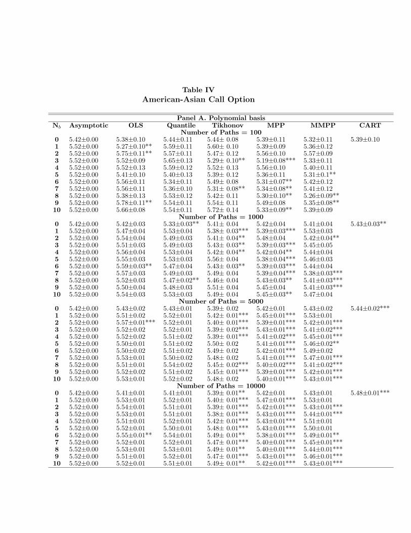
Table IVAmerican-Asian Call Option

Panel A. Polynomial basisNb Asymptotic OLS Quantile Tikhonov MPP MMPP CART

Number of Paths = 1000 5.42±0.00 5.38±0.10 5.44±0.11 5.44± 0.08 5.39±0.11 5.32±0.11 5.39±0.101 5.52±0.00 5.27±0.10** 5.59±0.11 5.60± 0.10 5.39±0.09 5.36±0.122 5.52±0.00 5.75±0.11** 5.57±0.11 5.47± 0.12 5.56±0.10 5.57±0.093 5.52±0.00 5.52±0.09 5.65±0.13 5.29± 0.10** 5.19±0.08*** 5.33±0.114 5.52±0.00 5.52±0.13 5.59±0.12 5.52± 0.13 5.56±0.10 5.40±0.115 5.52±0.00 5.41±0.10 5.40±0.13 5.39± 0.12 5.36±0.11 5.31±0.1**6 5.52±0.00 5.56±0.11 5.34±0.11 5.49± 0.08 5.31±0.07** 5.42±0.127 5.52±0.00 5.56±0.11 5.36±0.10 5.31± 0.08** 5.34±0.08** 5.41±0.128 5.52±0.00 5.38±0.13 5.53±0.12 5.42± 0.11 5.30±0.10** 5.26±0.09**9 5.52±0.00 5.78±0.11** 5.54±0.11 5.54± 0.11 5.49±0.08 5.35±0.08**10 5.52±0.00 5.66±0.08 5.54±0.11 5.72± 0.14 5.33±0.09** 5.39±0.09

Number of Paths = 10000 5.42±0.00 5.42±0.03 5.33±0.03** 5.41± 0.04 5.42±0.04 5.41±0.04 5.43±0.03**1 5.52±0.00 5.47±0.04 5.53±0.04 5.38± 0.03*** 5.39±0.03*** 5.53±0.032 5.52±0.00 5.54±0.04 5.49±0.03 5.41± 0.04** 5.48±0.04 5.42±0.04**3 5.52±0.00 5.51±0.03 5.49±0.03 5.43± 0.03** 5.39±0.03*** 5.45±0.054 5.52±0.00 5.56±0.04 5.53±0.04 5.42± 0.04** 5.42±0.04** 5.44±0.045 5.52±0.00 5.55±0.03 5.53±0.03 5.56± 0.04 5.38±0.04*** 5.46±0.036 5.52±0.00 5.59±0.03** 5.47±0.04 5.43± 0.03** 5.39±0.03*** 5.44±0.047 5.52±0.00 5.57±0.03 5.49±0.03 5.49± 0.04 5.39±0.04*** 5.38±0.03***8 5.52±0.00 5.52±0.03 5.47±0.02** 5.46± 0.04 5.43±0.03** 5.41±0.03***9 5.52±0.00 5.50±0.04 5.48±0.03 5.51± 0.04 5.45±0.04 5.41±0.03***10 5.52±0.00 5.54±0.03 5.53±0.03 5.49± 0.04 5.45±0.03** 5.47±0.04

Number of Paths = 50000 5.42±0.00 5.43±0.02 5.43±0.01 5.39± 0.02 5.42±0.01 5.43±0.02 5.44±0.02***1 5.52±0.00 5.51±0.02 5.52±0.01 5.42± 0.01*** 5.45±0.01*** 5.53±0.012 5.52±0.00 5.57±0.01*** 5.52±0.01 5.40± 0.01*** 5.39±0.01*** 5.42±0.01***3 5.52±0.00 5.52±0.02 5.52±0.01 5.39± 0.02*** 5.43±0.01*** 5.41±0.02***4 5.52±0.00 5.52±0.02 5.51±0.02 5.39± 0.01*** 5.41±0.02*** 5.45±0.01***5 5.52±0.00 5.50±0.01 5.51±0.02 5.50± 0.02 5.41±0.01*** 5.46±0.02**6 5.52±0.00 5.50±0.02 5.51±0.02 5.49± 0.02 5.42±0.01*** 5.49±0.027 5.52±0.00 5.53±0.01 5.50±0.02 5.48± 0.02 5.41±0.01*** 5.47±0.01***8 5.52±0.00 5.51±0.01 5.54±0.02 5.45± 0.02*** 5.40±0.02*** 5.41±0.02***9 5.52±0.00 5.52±0.02 5.51±0.02 5.45± 0.01*** 5.39±0.01*** 5.42±0.01***10 5.52±0.00 5.53±0.01 5.52±0.02 5.48± 0.02 5.40±0.01*** 5.43±0.01***

Number of Paths = 100000 5.42±0.00 5.41±0.01 5.41±0.01 5.39± 0.01** 5.42±0.01 5.43±0.01 5.48±0.01***1 5.52±0.00 5.53±0.01 5.52±0.01 5.40± 0.01*** 5.47±0.01*** 5.53±0.012 5.52±0.00 5.54±0.01 5.51±0.01 5.39± 0.01*** 5.42±0.01*** 5.43±0.01***3 5.52±0.00 5.53±0.01 5.51±0.01 5.38± 0.01*** 5.43±0.01*** 5.44±0.01***4 5.52±0.00 5.51±0.01 5.52±0.01 5.42± 0.01*** 5.43±0.01*** 5.51±0.015 5.52±0.00 5.52±0.01 5.50±0.01 5.48± 0.01*** 5.43±0.01*** 5.50±0.016 5.52±0.00 5.55±0.01** 5.54±0.01 5.49± 0.01** 5.38±0.01*** 5.49±0.01**7 5.52±0.00 5.52±0.01 5.52±0.01 5.47± 0.01*** 5.40±0.01*** 5.45±0.01***8 5.52±0.00 5.53±0.01 5.53±0.01 5.49± 0.01** 5.40±0.01*** 5.44±0.01***9 5.52±0.00 5.51±0.01 5.52±0.01 5.47± 0.01*** 5.43±0.01*** 5.46±0.01***10 5.52±0.00 5.52±0.01 5.51±0.01 5.49± 0.01** 5.42±0.01*** 5.43±0.01***

Panel B. Polynomial and European price basisNb Asymptotic OLS Quantile Tikhonov MPP MMPP CART

Number of Paths = 1000 5.78±0.00 5.84±0.07 5.81±0.10 5.89± 0.09 5.74±0.12 5.73±0.12 5.50±0.11**1 5.78±0.00 5.73±0.12 5.93±0.09 5.84± 0.12 5.77±0.10 5.68±0.112 5.78±0.00 5.71±0.10 5.78±0.12 5.80± 0.09 5.66±0.11 5.72±0.103 5.78±0.00 5.73±0.09 5.75±0.11 5.81± 0.08 5.58±0.10 5.96±0.104 5.78±0.00 5.88±0.14 5.68±0.14 5.79± 0.08 5.74±0.09 5.89±0.125 5.78±0.00 5.84±0.08 5.97±0.13 5.75± 0.08 5.84±0.12 5.91±0.156 5.78±0.00 5.78±0.10 5.63±0.13 5.94± 0.14 5.76±0.08 5.88±0.167 5.79±0.00 5.63±0.10 5.80±0.10 5.76± 0.11 5.72±0.10 5.56±0.09**8 5.78±0.00 5.86±0.09 5.91±0.11 5.82± 0.10 5.81±0.09 5.76±0.119 5.79±0.00 5.88±0.11 5.76±0.13 5.60± 0.10 5.70±0.12 5.76±0.1310 5.78±0.00 5.83±0.09 5.90±0.09 5.75± 0.08 5.75±0.09 5.69±0.11

Number of Paths = 10000 5.78±0.00 5.76±0.03 5.78±0.03 5.81± 0.02 5.81±0.03 5.76±0.03 5.48±0.03***1 5.78±0.00 5.82±0.04 5.77±0.03 5.74± 0.03 5.80±0.04 5.77±0.032 5.78±0.00 5.78±0.04 5.69±0.04** 5.74± 0.03 5.81±0.03 5.76±0.033 5.78±0.00 5.79±0.03 5.80±0.04 5.72± 0.03 5.75±0.03 5.78±0.024 5.78±0.00 5.82±0.03 5.73±0.03 5.80± 0.03 5.82±0.04 5.74±0.045 5.78±0.00 5.78±0.04 5.77±0.03 5.79± 0.03 5.76±0.04 5.77±0.036 5.78±0.00 5.81±0.04 5.73±0.03 5.77± 0.04 5.82±0.04 5.76±0.037 5.79±0.00 5.70±0.02*** 5.82±0.04 5.78± 0.03 5.72±0.03** 5.81±0.038 5.78±0.00 5.79±0.03 5.81±0.03 5.81± 0.04 5.79±0.03 5.77±0.039 5.79±0.00 5.80±0.03 5.83±0.03 5.77± 0.04 5.76±0.04 5.78±0.0310 5.78±0.00 5.81±0.03 5.86±0.04 5.81± 0.03 5.77±0.04 5.74±0.03

Number of Paths = 50000 5.78±0.00 5.78±0.02 5.79±0.02 5.80± 0.02 5.78±0.01 5.78±0.02 5.44±0.02***1 5.78±0.00 5.80±0.02 5.78±0.02 5.79± 0.02 5.79±0.02 5.81±0.022 5.78±0.00 5.78±0.01 5.76±0.01 5.78± 0.01 5.76±0.02 5.77±0.023 5.78±0.00 5.77±0.02 5.79±0.02 5.80± 0.02 5.77±0.01 5.78±0.014 5.78±0.00 5.78±0.02 5.76±0.01 5.77± 0.01 5.78±0.02 5.80±0.015 5.78±0.00 5.76±0.01 5.76±0.01 5.80± 0.01 5.80±0.02 5.81±0.01**6 5.78±0.00 5.77±0.01 5.75±0.01** 5.78± 0.02 5.79±0.02 5.75±0.027 5.79±0.00 5.80±0.02 5.78±0.01 5.78± 0.02 5.81±0.01 5.79±0.028 5.78±0.00 5.80±0.02 5.81±0.02 5.79± 0.02 5.77±0.02 5.77±0.029 5.79±0.00 5.77±0.01 5.77±0.01 5.76± 0.02 5.79±0.01 5.77±0.0110 5.78±0.00 5.77±0.01 5.74±0.01*** 5.77±0.02 5.78±0.01 5.77±0.02

Number of Paths = 100000 5.78±0.00 5.80±0.01 5.75±0.01** 5.81± 0.01** 5.79±0.01 5.79±0.01 5.45±0.01***1 5.78±0.00 5.78±0.01 5.78±0.01 5.79± 0.01 5.78±0.01 5.77±0.012 5.78±0.00 5.77±0.01 5.76±0.01 5.77± 0.01 5.78±0.01 5.78±0.013 5.78±0.00 5.79±0.01 5.77±0.01 5.78± 0.01 5.78±0.01 5.78±0.014 5.78±0.00 5.78±0.01 5.76±0.01 5.79± 0.01 5.78±0.01 5.80±0.015 5.78±0.00 5.76±0.01 5.78±0.01 5.78± 0.01 5.79±0.01 5.78±0.016 5.78±0.00 5.78±0.01 5.78±0.01 5.81± 0.01** 5.78±0.01 5.78±0.017 5.79±0.00 5.77±0.01 5.77±0.01 5.78± 0.01 5.77±0.01 5.81±0.018 5.78±0.00 5.79±0.01 5.77±0.01 5.79± 0.01 5.79±0.01 5.79±0.019 5.79±0.00 5.79±0.01 5.78±0.01 5.77± 0.01 5.78±0.01 5.78±0.0110 5.78±0.00 5.78±0.01 5.78±0.01 5.77± 0.01 5.79±0.01 5.77±0.01

Notes: The parameters are: σ = 0.2, r = 0.09, T = 120/365, t′ = 91/365, S0 = 100, K =100, and exercise points t ∈ {0, 105/365, 108/365, 111/365, 114/365, 117/365, 120/365}.Nb denotes the highest degree of the polynomial basis functions. The standard errors arereported after the ± sign based on 20 replications. The asymptotic value is computedby the OLS regression method with 100,000 paths. The “**” sign means two to threestandard errors away from the asymptotic value. The “***” sign means more than threestandard errors away.

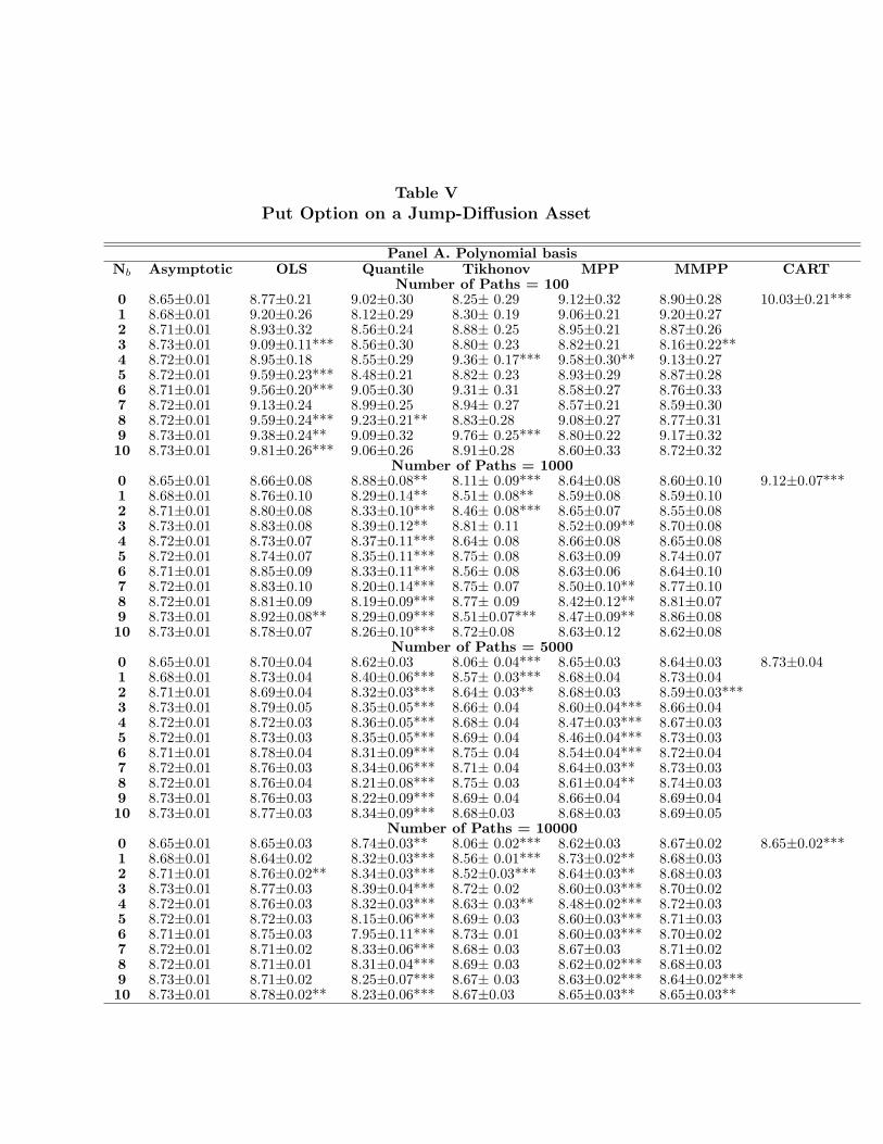
Table VPut Option on a Jump-Diffusion Asset

Panel A. Polynomial basisNb Asymptotic OLS Quantile Tikhonov MPP MMPP CART

Number of Paths = 1000 8.65±0.01 8.77±0.21 9.02±0.30 8.25± 0.29 9.12±0.32 8.90±0.28 10.03±0.21***1 8.68±0.01 9.20±0.26 8.12±0.29 8.30± 0.19 9.06±0.21 9.20±0.272 8.71±0.01 8.93±0.32 8.56±0.24 8.88± 0.25 8.95±0.21 8.87±0.263 8.73±0.01 9.09±0.11*** 8.56±0.30 8.80± 0.23 8.82±0.21 8.16±0.22**4 8.72±0.01 8.95±0.18 8.55±0.29 9.36± 0.17*** 9.58±0.30** 9.13±0.275 8.72±0.01 9.59±0.23*** 8.48±0.21 8.82± 0.23 8.93±0.29 8.87±0.286 8.71±0.01 9.56±0.20*** 9.05±0.30 9.31± 0.31 8.58±0.27 8.76±0.337 8.72±0.01 9.13±0.24 8.99±0.25 8.94± 0.27 8.57±0.21 8.59±0.308 8.72±0.01 9.59±0.24*** 9.23±0.21** 8.83±0.28 9.08±0.27 8.77±0.319 8.73±0.01 9.38±0.24** 9.09±0.32 9.76± 0.25*** 8.80±0.22 9.17±0.3210 8.73±0.01 9.81±0.26*** 9.06±0.26 8.91±0.28 8.60±0.33 8.72±0.32

Number of Paths = 10000 8.65±0.01 8.66±0.08 8.88±0.08** 8.11± 0.09*** 8.64±0.08 8.60±0.10 9.12±0.07***1 8.68±0.01 8.76±0.10 8.29±0.14** 8.51± 0.08** 8.59±0.08 8.59±0.102 8.71±0.01 8.80±0.08 8.33±0.10*** 8.46± 0.08*** 8.65±0.07 8.55±0.083 8.73±0.01 8.83±0.08 8.39±0.12** 8.81± 0.11 8.52±0.09** 8.70±0.084 8.72±0.01 8.73±0.07 8.37±0.11*** 8.64± 0.08 8.66±0.08 8.65±0.085 8.72±0.01 8.74±0.07 8.35±0.11*** 8.75± 0.08 8.63±0.09 8.74±0.076 8.71±0.01 8.85±0.09 8.33±0.11*** 8.56± 0.08 8.63±0.06 8.64±0.107 8.72±0.01 8.83±0.10 8.20±0.14*** 8.75± 0.07 8.50±0.10** 8.77±0.108 8.72±0.01 8.81±0.09 8.19±0.09*** 8.77± 0.09 8.42±0.12** 8.81±0.079 8.73±0.01 8.92±0.08** 8.29±0.09*** 8.51±0.07*** 8.47±0.09** 8.86±0.0810 8.73±0.01 8.78±0.07 8.26±0.10*** 8.72±0.08 8.63±0.12 8.62±0.08

Number of Paths = 50000 8.65±0.01 8.70±0.04 8.62±0.03 8.06± 0.04*** 8.65±0.03 8.64±0.03 8.73±0.041 8.68±0.01 8.73±0.04 8.40±0.06*** 8.57± 0.03*** 8.68±0.04 8.73±0.042 8.71±0.01 8.69±0.04 8.32±0.03*** 8.64± 0.03** 8.68±0.03 8.59±0.03***3 8.73±0.01 8.79±0.05 8.35±0.05*** 8.66± 0.04 8.60±0.04*** 8.66±0.044 8.72±0.01 8.72±0.03 8.36±0.05*** 8.68± 0.04 8.47±0.03*** 8.67±0.035 8.72±0.01 8.73±0.03 8.35±0.05*** 8.69± 0.04 8.46±0.04*** 8.73±0.036 8.71±0.01 8.78±0.04 8.31±0.09*** 8.75± 0.04 8.54±0.04*** 8.72±0.047 8.72±0.01 8.76±0.03 8.34±0.06*** 8.71± 0.04 8.64±0.03** 8.73±0.038 8.72±0.01 8.76±0.04 8.21±0.08*** 8.75± 0.03 8.61±0.04** 8.74±0.039 8.73±0.01 8.76±0.03 8.22±0.09*** 8.69± 0.04 8.66±0.04 8.69±0.0410 8.73±0.01 8.77±0.03 8.34±0.09*** 8.68±0.03 8.68±0.03 8.69±0.05

Number of Paths = 100000 8.65±0.01 8.65±0.03 8.74±0.03** 8.06± 0.02*** 8.62±0.03 8.67±0.02 8.65±0.02***1 8.68±0.01 8.64±0.02 8.32±0.03*** 8.56± 0.01*** 8.73±0.02** 8.68±0.032 8.71±0.01 8.76±0.02** 8.34±0.03*** 8.52±0.03*** 8.64±0.03** 8.68±0.033 8.73±0.01 8.77±0.03 8.39±0.04*** 8.72± 0.02 8.60±0.03*** 8.70±0.024 8.72±0.01 8.76±0.03 8.32±0.03*** 8.63± 0.03** 8.48±0.02*** 8.72±0.035 8.72±0.01 8.72±0.03 8.15±0.06*** 8.69± 0.03 8.60±0.03*** 8.71±0.036 8.71±0.01 8.75±0.03 7.95±0.11*** 8.73± 0.01 8.60±0.03*** 8.70±0.027 8.72±0.01 8.71±0.02 8.33±0.06*** 8.68± 0.03 8.67±0.03 8.71±0.028 8.72±0.01 8.71±0.01 8.31±0.04*** 8.69± 0.03 8.62±0.02*** 8.68±0.039 8.73±0.01 8.71±0.02 8.25±0.07*** 8.67± 0.03 8.63±0.02*** 8.64±0.02***10 8.73±0.01 8.78±0.02** 8.23±0.06*** 8.67±0.03 8.65±0.03** 8.65±0.03**

Panel B. Polynomial and European price basisNb Asymptotic OLS Quantile Tikhonov MPP MMPP CART

Number of Paths = 1000 8.72±0.01 9.74±0.25*** 9.60±0.29*** 9.10±0.34 9.49±0.17*** 9.10±0.27 9.55±0.24***1 8.72±0.01 9.94±0.23*** 9.62±0.27*** 8.71±0.27 8.84±0.23 9.05±0.262 8.72±0.01 10.32±0.24*** 9.41±0.30** 8.92±0.25 9.03±0.24 8.90±0.283 8.73±0.01 9.55±0.19*** 9.34±0.31 9.09± 0.23 9.07±0.28 9.15±0.314 8.72±0.01 9.29±0.23** 9.84±0.21*** 8.90±0.17 8.90±0.25 9.66±0.22***5 8.72±0.01 10.03±0.32*** 9.56±0.28** 9.61±0.30** 9.35±0.23** 9.02±0.296 8.71±0.01 9.77±0.26*** 9.80±0.31*** 9.21±0.18** 8.66±0.23 8.83±0.277 8.72±0.01 10.17±0.21*** 9.73±0.32*** 9.13±0.21 9.17±0.24 8.74±0.338 8.73±0.01 9.36±0.29** 9.65±0.24*** 8.58±0.18 9.09±0.26 9.44±0.24**9 8.72±0.01 10.14±0.24*** 9.90±0.28*** 9.28±0.20** 9.47±0.28** 8.91±0.2210 8.73±0.01 9.54±0.31** 9.49±0.29** 8.78±0.30 9.33±0.21** 8.89±0.28

Number of Paths = 10000 8.72±0.01 8.83±0.09 8.44±0.08*** 8.81± 0.07 8.72±0.08 8.73±0.07 9.12±0.10***1 8.72±0.01 8.91±0.07** 8.31±0.11*** 8.70±0.08 8.65±0.08 8.64±0.082 8.72±0.01 8.92±0.10 8.59±0.10 8.75± 0.07 8.79±0.08 8.69±0.083 8.73±0.01 8.82±0.09 8.49±0.10** 8.81± 0.08 8.61±0.08 8.78±0.084 8.72±0.01 8.94±0.07*** 8.54±0.12 8.79± 0.07 8.80±0.10 8.63±0.065 8.72±0.01 8.97±0.07*** 8.53±0.08** 8.72±0.06 8.58±0.06** 8.92±0.07**6 8.71±0.01 8.82±0.09 8.68±0.09 8.77± 0.06 8.72±0.09 8.79±0.107 8.72±0.01 9.01±0.11** 8.58±0.12 8.77± 0.08 8.63±0.07 8.60±0.108 8.73±0.01 8.94±0.08** 8.57±0.10 8.75± 0.08 8.61±0.07 8.69±0.109 8.72±0.01 8.92±0.08** 8.70±0.11 8.82± 0.07 8.60±0.08 8.78±0.0910 8.73±0.01 9.09±0.06*** 8.75±0.09 8.83±0.09 8.96±0.08** 8.64±0.07

Number of Paths = 50000 8.72±0.01 8.73±0.04 8.41±0.05*** 8.68± 0.04 8.69±0.04 8.71±0.03 8.77±0.041 8.72±0.01 8.74±0.03 8.39±0.05*** 8.72± 0.03 8.64±0.03** 8.72±0.042 8.72±0.01 8.68±0.04 8.49±0.04*** 8.71± 0.03 8.65±0.04 8.69±0.033 8.73±0.01 8.76±0.04 8.42±0.06*** 8.73± 0.04 8.62±0.03*** 8.72±0.044 8.72±0.01 8.68±0.03 8.38±0.08*** 8.71± 0.04 8.70±0.04 8.75±0.045 8.72±0.01 8.74±0.04 8.46±0.06*** 8.74± 0.03 8.68±0.03 8.66±0.02**6 8.71±0.01 8.82±0.04** 8.45±0.05*** 8.78±0.02*** 8.64±0.03** 8.64±0.057 8.72±0.01 8.74±0.04 8.51±0.05*** 8.78± 0.03 8.69±0.05 8.70±0.038 8.73±0.01 8.77±0.03 8.49±0.05*** 8.71± 0.03 8.75±0.03 8.69±0.039 8.72±0.01 8.76±0.03 8.45±0.06*** 8.74± 0.03 8.71±0.04 8.79±0.03**10 8.73±0.01 8.78±0.03 8.46±0.05*** 8.73±0.03 8.67±0.03 8.79±0.04

Number of Paths = 100000 8.72±0.01 8.74±0.03 8.33±0.04*** 8.71± 0.03 8.69±0.02 8.67±0.02** 8.66±0.02***1 8.72±0.01 8.75±0.02 8.39±0.04*** 8.75± 0.03 8.71±0.03 8.68±0.022 8.72±0.01 8.74±0.03 8.42±0.06*** 8.75± 0.02 8.71±0.03 8.74±0.023 8.73±0.01 8.78±0.02** 8.50±0.04*** 8.71±0.03 8.66±0.02*** 8.73±0.024 8.72±0.01 8.77±0.03 8.42±0.06*** 8.73± 0.03 8.67±0.02** 8.76±0.025 8.72±0.01 8.75±0.03 8.35±0.04*** 8.77± 0.03 8.74±0.03 8.71±0.026 8.71±0.01 8.74±0.02 8.43±0.04*** 8.71± 0.02 8.75±0.02 8.70±0.037 8.72±0.01 8.71±0.03 8.48±0.05*** 8.69± 0.02 8.65±0.03** 8.71±0.028 8.73±0.01 8.74±0.02 8.49±0.04*** 8.75± 0.03 8.73±0.02 8.75±0.029 8.72±0.01 8.71±0.02 8.47±0.05*** 8.71± 0.02 8.68±0.02 8.69±0.0310 8.73±0.01 8.75±0.03 8.47±0.04*** 8.75±0.02 8.71±0.02 8.73±0.03

Notes: The parameters are: σ =√

0.08, r = 0.1, T = 0.5, δ = 0.2, S0 = 100, K =100, λ = 2, and exercise points t ∈ {0, 0.125, 0.25, 0.375, 0.5}. Nb denotes the highestdegree of the polynomial basis functions. The standard errors are reported after the ±sign based on 20 replications. The asymptotic value is computed by the OLS regressionmethod with 100,000 paths. The “**” sign means two to three standard errors awayfrom the asymptotic value. The “***” sign means more than three standard errors away.

Table VIMax-Call Option on Two Assets

Panel A. K=80, polynomial basisNb Asymptotic OLS Quantile Tikhonov MPP MMPP CART

Number of Paths = 1000 24.82±0.00 25.81±0.18*** 25.16±0.15** 23.67 ±0.21*** 23.87±0.23*** 25.20±0.21 25.54±0.17***1 24.82±0.01 26.08±0.22*** 25.71±0.25*** 25.97±0.18*** 23.59±0.16*** 25.73±0.20***2 24.87±0.00 26.86±0.17*** 25.50±0.22** 26.41 ±0.12*** 24.77±0.23 25.75±0.20***3 24.98±0.01 26.49±0.15*** 25.90±0.21*** 25.99±0.19*** 24.91±0.23 26.10±0.19***4 25.00±0.01 27.35±0.19*** 26.28±0.23*** 26.51±0.20*** 25.33±0.18 25.57±0.16***5 25.00±0.00 27.88±0.21*** 25.94±0.20*** 26.78±0.18*** 25.21±0.19 25.74±0.13***

Number of Paths = 10000 24.82±0.00 24.88±0.05 24.77±0.05 23.74±0.06*** 23.78±0.06*** 24.84±0.06 23.87±0.06***1 24.82±0.01 25.04±0.04*** 24.83±0.05 24.91±0.05 23.83±0.05*** 24.96±0.06**2 24.87±0.00 25.30±0.05*** 24.95±0.06 25.12±0.05*** 24.73±0.05** 25.00±0.05**3 24.98±0.01 25.17±0.06*** 25.08±0.06 25.07±0.06 24.59±0.07*** 24.99±0.054 25.00±0.01 25.31±0.07*** 25.18±0.05*** 25.23±0.05*** 24.80±0.06*** 24.81±0.05***5 25.00±0.00 25.45±0.06*** 25.07±0.06 25.03±0.04 24.80±0.05*** 24.82±0.07**

Number of Paths = 50000 24.82±0.00 24.82±0.03 24.67±0.03*** 23.71±0.02*** 24.00±0.03*** 24.85±0.03 23.71±0.02***1 24.82±0.01 24.87±0.02** 24.73±0.02*** 24.84 ±0.02 24.03±0.03*** 24.90±0.03**2 24.87±0.00 25.01±0.03*** 24.73±0.03*** 24.96±0.03** 24.79±0.03** 24.88±0.023 24.98±0.01 25.06±0.02*** 24.90±0.02*** 24.97±0.03 24.76±0.02*** 24.92±0.034 25.00±0.01 25.05±0.02** 24.88±0.02*** 24.97 ±0.02 24.80±0.03*** 24.88±0.02***5 25.00±0.00 25.14±0.03*** 24.94±0.02** 24.98 ±0.03 24.80±0.03*** 24.91±0.03**

Number of Paths = 100000 24.82±0.00 24.84±0.02 24.65±0.02*** 23.69±0.02*** 24.27±0.02*** 24.84±0.02 23.70±0.02***1 24.82±0.01 24.85±0.02 24.67±0.02*** 24.86±0.02 24.23±0.01*** 24.82±0.022 24.87±0.00 24.93±0.02** 24.70±0.01*** 24.92 ±0.02** 24.85±0.01 24.91±0.023 24.98±0.01 25.00±0.02 24.82±0.02*** 24.94±0.02 24.81±0.02*** 24.91±0.02***4 25.00±0.01 25.04±0.01*** 24.88±0.02*** 24.95±0.02** 24.80±0.02*** 24.88±0.02***5 25.00±0.00 25.04±0.02 24.84±0.01*** 24.93±0.02*** 24.73±0.02*** 24.93±0.02***

Panel B. K=80, polynomial and European price basisNb Asymptotic OLS Quantile Tikhonov MPP MMPP CART

Number of Paths = 1000 25.03±0.00 26.88±0.15*** 26.03±0.18*** 25.26±0.18 25.69±0.16*** 26.02±0.19*** 25.62±0.21**1 25.03±0.01 27.76±0.17*** 26.94±0.27*** 25.83±0.19*** 26.04±0.23*** 25.81±0.11***2 25.04±0.01 28.08±0.19*** 26.89±0.17*** 26.19±0.18*** 25.73±0.17*** 26.06±0.16***3 25.03±0.00 27.82±0.16*** 27.13±0.16*** 26.22±0.19*** 25.69±0.23** 26.33±0.20***4 25.03±0.01 28.47±0.20*** 27.35±0.25*** 26.16±0.22*** 25.80±0.20*** 26.17±0.21***5 25.04±0.01 28.73±0.21*** 27.88±0.19*** 26.00±0.16*** 25.93±0.27*** 26.02±0.18***

Number of Paths = 10000 25.03±0.00 24.99±0.05 25.38±0.06*** 25.09±0.05 25.09±0.05 25.09±0.04 23.60±0.06***1 25.03±0.01 25.29±0.05*** 25.47±0.05*** 25.02±0.04 25.05±0.05 25.10±0.042 25.04±0.01 25.18±0.06** 25.50±0.06*** 25.19 ±0.05** 25.03±0.05 25.16±0.05**3 25.03±0.00 25.33±0.04*** 25.55±0.04*** 25.09±0.05 25.08±0.05 25.13±0.054 25.03±0.01 25.36±0.06*** 25.58±0.06*** 25.07±0.06 25.05±0.04 25.21±0.05***5 25.04±0.01 25.46±0.08*** 25.66±0.05*** 25.10±0.05 25.02±0.04 25.20±0.05***

Number of Paths = 50000 25.03±0.00 24.90±0.03*** 25.13±0.03*** 25.00±0.02 25.00±0.02 25.05±0.02 23.69±0.03***1 25.03±0.01 24.90±0.03*** 25.12±0.02*** 25.03±0.02 25.04±0.02 25.06±0.022 25.04±0.01 24.99±0.03 25.14±0.03*** 25.02±0.03 25.02±0.02 25.06±0.023 25.03±0.00 24.97±0.03 25.16±0.02*** 25.00±0.02 24.99±0.02 25.05±0.024 25.03±0.01 24.98±0.03 25.14±0.03*** 25.04±0.02 24.99±0.02 25.08±0.02**5 25.04±0.01 25.01±0.02 25.16±0.02*** 25.04±0.02 25.00±0.02 25.04±0.02

Number of Paths = 100000 25.03±0.00 24.82±0.01*** 25.08±0.02** 25.00 ±0.02 25.03±0.01 25.02±0.02 23.68±0.02***1 25.03±0.01 24.85±0.02*** 25.08±0.01*** 25.01±0.02 25.00±0.01** 25.03±0.012 25.04±0.01 24.85±0.02*** 25.10±0.02** 25.03 ±0.02 25.00±0.02 25.02±0.023 25.03±0.00 24.89±0.02*** 25.10±0.01*** 25.01±0.02 25.04±0.01 25.04±0.024 25.03±0.01 24.89±0.02*** 25.10±0.02*** 25.05±0.01 25.03±0.01 25.05±0.015 25.04±0.01 24.89±0.02*** 25.09±0.01*** 25.04±0.01 25.03±0.02 25.05±0.01

Panel C. K=100, polynomial basisNb Asymptotic OLS Quantile Tikhonov MPP MMPP CART

Number of Paths = 1000 9.43±0.01 10.01±0.22** 8.99±0.23 8.48± 0.15*** 8.97±0.16** 9.20±0.19 9.98±0.15**1 9.43±0.00 10.79±0.19*** 9.25±0.19 9.63±0.22 8.98±0.16** 9.45±0.182 9.51±0.00 11.27±0.22*** 10.23±0.17*** 10.33 ±0.18*** 9.21±0.18 9.58±0.203 9.52±0.01 11.41±0.20*** 9.98±0.29 10.76±0.11*** 9.49±0.12 9.73±0.164 9.52±0.01 11.57±0.14*** 9.79±0.24 11.24±0.19*** 9.16±0.15** 9.85±0.235 9.53±0.01 11.58±0.21*** 9.65±0.16 10.93±0.21*** 9.87±0.25 10.07±0.16***

Number of Paths = 10000 9.43±0.01 9.48±0.05 9.22±0.07** 8.75± 0.05*** 8.82±0.06*** 9.37±0.07 8.86±0.06***1 9.43±0.00 9.59±0.08 9.13±0.07*** 9.53± 0.04** 8.89±0.05*** 9.39±0.082 9.51±0.00 9.70±0.06*** 9.33±0.08** 9.67±0.08 9.12±0.06*** 9.58±0.063 9.52±0.01 9.80±0.07*** 9.37±0.08 9.72± 0.06*** 9.16±0.04*** 9.55±0.074 9.52±0.01 9.86±0.06*** 9.41±0.07 9.70± 0.06** 9.25±0.04*** 9.54±0.075 9.53±0.01 9.91±0.06*** 9.43±0.06 9.68± 0.05** 9.27±0.05*** 9.51±0.05

Number of Paths = 50000 9.43±0.01 9.44±0.03 9.20±0.02*** 8.73± 0.02*** 8.96±0.03*** 9.47±0.03 8.72±0.02***1 9.43±0.00 9.49±0.02** 9.23±0.03*** 9.40±0.04 8.99±0.03*** 9.42±0.032 9.51±0.00 9.56±0.02** 9.37±0.02*** 9.53±0.03 9.26±0.02*** 9.50±0.033 9.52±0.01 9.58±0.03 9.39±0.03*** 9.57± 0.03 9.27±0.02*** 9.51±0.034 9.52±0.01 9.58±0.02** 9.39±0.03*** 9.56±0.02 9.34±0.03*** 9.49±0.035 9.53±0.01 9.59±0.03 9.37±0.03*** 9.55± 0.02 9.31±0.01*** 9.53±0.02

Number of Paths = 100000 9.43±0.01 9.45±0.02 9.24±0.02*** 8.72± 0.01*** 9.04±0.02*** 9.43±0.02 8.78±0.02***1 9.43±0.00 9.44±0.02 9.21±0.02*** 9.43± 0.02 9.05±0.02*** 9.43±0.022 9.51±0.00 9.52±0.02 9.37±0.02*** 9.55± 0.02 9.31±0.02*** 9.53±0.023 9.52±0.01 9.54±0.02 9.33±0.02*** 9.50± 0.02 9.31±0.01*** 9.52±0.024 9.52±0.01 9.60±0.02*** 9.38±0.02*** 9.53±0.02 9.32±0.03*** 9.49±0.025 9.53±0.01 9.54±0.02 9.34±0.03*** 9.56± 0.01** 9.38±0.02*** 9.52±0.02

Panel D. K=100, polynomial and European price basisNb Asymptotic OLS Quantile Tikhonov MPP MMPP CART

Number of Paths = 1000 9.55±0.01 11.64±0.18*** 10.18±0.22** 10.10±0.23** 10.26±0.16*** 10.34±0.23*** 9.74±0.201 9.57±0.01 11.84±0.18*** 10.65±0.18*** 10.82 ±0.19*** 10.14±0.21** 10.67±0.15***2 9.56±0.01 12.21±0.19*** 11.06±0.18*** 10.52 ±0.18*** 9.97±0.16** 10.50±0.19***3 9.57±0.01 12.30±0.18*** 11.60±0.17*** 10.88 ±0.20*** 9.93±0.21 10.49±0.22***4 9.57±0.00 12.23±0.21*** 11.62±0.16*** 10.88 ±0.14*** 9.90±0.18 10.16±0.16***5 9.56±0.01 12.47±0.20*** 11.86±0.26*** 10.93 ±0.20*** 10.01±0.17** 10.81±0.24***

Number of Paths = 10000 9.55±0.01 10.00±0.07*** 9.33±0.09** 9.64±0.06 9.59±0.05 9.60±0.04 8.95±0.07***1 9.57±0.01 9.98±0.06*** 9.55±0.05 9.68± 0.07 9.68±0.06 9.61±0.072 9.56±0.01 10.13±0.05*** 9.62±0.05 9.66±0.08 9.53±0.05 9.69±0.06**3 9.57±0.01 10.12±0.06*** 9.68±0.07 9.66±0.07 9.72±0.07** 9.60±0.054 9.57±0.00 10.15±0.06*** 9.79±0.06*** 9.58±0.06 9.63±0.06 9.61±0.075 9.56±0.01 10.25±0.06*** 9.75±0.08** 9.68±0.06 9.50±0.04 9.69±0.06**

Number of Paths = 50000 9.55±0.01 9.65±0.02*** 9.33±0.04*** 9.53±0.03 9.56±0.03 9.60±0.03 8.75±0.02***1 9.57±0.01 9.67±0.02*** 9.37±0.04*** 9.62±0.02** 9.55±0.02 9.60±0.032 9.56±0.01 9.70±0.02*** 9.38±0.04*** 9.59±0.03 9.56±0.02 9.59±0.033 9.57±0.01 9.71±0.02*** 9.45±0.03*** 9.57±0.03 9.57±0.02 9.57±0.024 9.57±0.00 9.69±0.02*** 9.49±0.02*** 9.53±0.03 9.55±0.03 9.61±0.035 9.56±0.01 9.74±0.02*** 9.45±0.03*** 9.59±0.02 9.59±0.03 9.56±0.02

Number of Paths = 100000 9.55±0.01 9.63±0.01*** 9.32±0.03*** 9.51±0.02 9.52±0.01** 9.56±0.02 8.76±0.01***1 9.57±0.01 9.61±0.02 9.34±0.03*** 9.55± 0.02 9.53±0.02 9.53±0.022 9.56±0.01 9.62±0.02** 9.35±0.03*** 9.54±0.02 9.53±0.02 9.57±0.013 9.57±0.01 9.62±0.02** 9.35±0.02*** 9.53±0.01*** 9.56±0.02 9.54±0.024 9.57±0.00 9.66±0.02*** 9.43±0.03*** 9.56±0.02 9.55±0.02 9.55±0.025 9.56±0.01 9.64±0.02*** 9.34±0.03*** 9.57±0.02 9.54±0.02 9.56±0.02

Panel E. K=110, polynomial basisNb Asymptotic OLS Quantile Tikhonov MPP MMPP CART

Number of Paths = 1000 4.95±0.00 5.81±0.19*** 4.37±0.37 4.65± 0.13** 5.12±0.15 4.91±0.18 5.12±0.091 Not enough in-the-money paths beyond this point

Number of Paths = 10000 4.95±0.00 4.98±0.06 4.62±0.07*** 4.75± 0.05*** 4.73±0.05*** 4.81±0.04*** 5.05±0.041 4.95±0.01 5.12±0.04*** 4.64±0.09*** 5.06±0.04** 4.81±0.05** 4.98±0.062 4.99±0.01 5.21±0.04*** 4.90±0.07 5.18± 0.06*** 4.89±0.03*** 5.02±0.063 4.99±0.00 5.19±0.06*** 4.69±0.06*** 5.15±0.05*** 4.82±0.04*** 5.07±0.054 4.99±0.00 5.18±0.05*** 4.77±0.06*** 5.15±0.06** 4.96±0.05 5.01±0.055 5.00±0.01 5.28±0.05*** 4.85±0.07** 5.18±0.06** 4.86±0.05** 4.95±0.05

Number of Paths = 50000 4.95±0.00 4.98±0.02 4.64±0.02*** 4.74± 0.02*** 4.80±0.02*** 4.94±0.03 4.71±0.02***1 4.95±0.01 4.98±0.02 4.74±0.03*** 4.98± 0.02 4.78±0.02*** 4.93±0.022 4.99±0.01 5.00±0.02 4.84±0.02*** 5.03± 0.02 4.87±0.02*** 4.97±0.023 4.99±0.00 5.06±0.02*** 4.78±0.02*** 5.02±0.02 4.89±0.02*** 4.98±0.024 4.99±0.00 5.03±0.02 4.79±0.02*** 5.05± 0.02** 4.86±0.02*** 5.06±0.02***5 5.00±0.01 5.07±0.02*** 4.77±0.03*** 5.06±0.02** 4.86±0.02*** 5.03±0.02

Number of Paths = 100000 4.95±0.00 4.99±0.02 4.73±0.03*** 4.70± 0.02*** 4.78±0.01*** 4.93±0.02 4.74±0.01***1 4.95±0.01 4.96±0.02 4.72±0.02*** 4.95± 0.02 4.82±0.02*** 4.95±0.022 4.99±0.01 4.99±0.02 4.80±0.02*** 5.02± 0.02 4.88±0.02*** 4.97±0.013 4.99±0.00 5.01±0.02 4.79±0.03*** 5.02± 0.02 4.86±0.01*** 4.99±0.014 4.99±0.00 5.02±0.02 4.80±0.02*** 5.03± 0.01*** 4.88±0.02*** 4.98±0.025 5.00±0.01 5.04±0.01*** 4.78±0.03*** 4.98±0.02 4.89±0.02*** 5.00±0.01

Panel F. K=110, polynomial and European price basisNb Asymptotic OLS Quantile Tikhonov MPP MMPP CART

Number of Paths = 1000 Not enough in-the-money paths beyond this point

Number of Paths = 10000 5.02±0.01 5.35±0.04*** 4.84±0.06** 5.03±0.05 5.08±0.04 5.10±0.04 5.06±0.041 5.02±0.00 5.45±0.06*** 4.95±0.06 5.19± 0.05*** 4.99±0.07 5.20±0.06**2 5.01±0.00 5.52±0.05*** 5.03±0.06 5.12± 0.05** 5.05±0.05 5.20±0.04***3 5.02±0.01 5.44±0.06*** 5.00±0.05 5.29± 0.06*** 5.10±0.05 5.04±0.044 5.02±0.01 5.43±0.05*** 5.08±0.06 5.15± 0.07 5.09±0.06 5.16±0.075 5.02±0.01 5.48±0.03*** 5.22±0.06*** 5.30±0.05*** 5.14±0.04** 5.19±0.05***

Number of Paths = 50000 5.02±0.01 5.08±0.02** 4.77±0.03*** 5.02±0.02 5.02±0.02 5.08±0.02** 4.78±0.02***1 5.02±0.00 5.14±0.02*** 4.87±0.03*** 5.05±0.02 5.04±0.03 5.05±0.022 5.01±0.00 5.14±0.02*** 4.92±0.03** 5.02±0.03 4.99±0.02 5.04±0.023 5.02±0.01 5.16±0.02*** 4.87±0.04*** 5.02±0.02 5.04±0.02 5.05±0.024 5.02±0.01 5.16±0.03*** 4.92±0.03*** 5.04±0.02 4.96±0.02** 5.05±0.035 5.02±0.01 5.16±0.03*** 4.92±0.03*** 5.02±0.02 5.01±0.01 5.06±0.03

Number of Paths = 100000 5.02±0.01 5.07±0.02** 4.77±0.02*** 5.01±0.01 5.03±0.01 5.03±0.01 4.73±0.02***1 5.02±0.00 5.06±0.01*** 4.83±0.02*** 5.02±0.02 5.03±0.01 5.03±0.012 5.01±0.00 5.07±0.02** 4.85±0.02*** 5.02±0.02 5.01±0.01 5.03±0.013 5.02±0.01 5.07±0.02** 4.85±0.03*** 5.02±0.02 5.00±0.02 5.02±0.024 5.02±0.01 5.09±0.02*** 4.85±0.03*** 5.03±0.01 4.98±0.02 5.02±0.025 5.02±0.01 5.09±0.02*** 4.86±0.02*** 4.99±0.01** 4.99±0.02 5.01±0.01

Notes: The parameters are: σ = 0.2, r = 0.05, T = 1, δ = 0.1, S0 = 100, ρ = 0.3, andexercise points t ∈ {0, 1/12, 2/12, . . . , 12/12}. Nb implicitly shows the number of basisfunctions according to Table I. The standard errors are reported after the ± sign basedon 20 replications. The asymptotic value is computed by the OLS regression methodwith 100,000 paths. The “**” sign means two to three standard errors away from theasymptotic value. The “***” sign means more than three standard errors away.

Table VIIMax-Call Option on Ten Assets

Panel A. K=80, polynomial basisNb Asymptotic OLS Quantile Tikhonov MPP MMPP CART

Number of Paths = 1000 40.38±0.01 41.09±0.24** 40.67±0.25 36.66±0.65*** 37.94±0.31*** 40.80±0.29 38.00±0.21***1 40.39±0.01 42.60±0.22*** 41.58±0.27*** 38.00±0.29*** 38.24±0.30*** 42.34±0.21***2 40.40±0.01 43.17±0.25*** 41.58±0.27*** 38.79±0.26*** 39.24±0.19*** 42.28±0.24***3 40.42±0.01 45.53±0.23*** 42.46±0.20*** 39.43±0.22*** 39.78±0.25** 41.76±0.26***4 40.41±0.00 46.74±0.25*** 43.54±0.24*** 40.18±0.24 39.76±0.26** 41.92±0.17***5 Not enough in-the-money paths beyond this point

Number of Paths = 10000 40.38±0.01 40.46±0.07 40.26±0.07 37.32±0.10*** 38.54±0.09*** 40.44±0.08 37.02±0.07***1 40.39±0.01 40.69±0.09*** 40.84±0.08*** 37.77±0.10*** 38.83±0.08*** 40.60±0.05***2 40.40±0.01 40.95±0.08*** 40.78±0.09*** 38.62±0.08*** 39.72±0.09*** 40.47±0.063 40.42±0.01 41.59±0.07*** 40.87±0.06*** 38.86±0.07*** 39.35±0.09*** 40.62±0.09**4 40.41±0.00 41.62±0.06*** 40.91±0.06*** 39.32±0.08*** 39.75±0.09*** 40.56±0.085 40.54±0.01 44.46±0.08*** 43.04±0.08*** 39.54±0.08*** 39.66±0.08*** 40.49±0.08

Number of Paths = 50000 40.38±0.01 40.40±0.03 40.41±0.04 37.25±0.04*** 39.97±0.04*** 40.42±0.03 36.95±0.05***1 40.39±0.01 40.44±0.03 40.43±0.03 37.79±0.04*** 39.98±0.04*** 40.47±0.03**2 40.40±0.01 40.46±0.03 40.49±0.03** 38.51±0.04*** 40.15±0.04*** 40.36±0.033 40.42±0.01 40.71±0.03*** 40.59±0.03*** 38.89±0.03*** 40.03±0.04*** 40.40±0.044 40.41±0.00 40.71±0.03*** 40.56±0.04*** 39.25±0.03*** 40.11±0.04*** 40.42±0.035 40.54±0.01 41.72±0.03*** 41.17±0.03*** 39.42±0.03*** 40.07±0.03*** 40.36±0.03***

Number of Paths = 100000 40.38±0.01 40.40±0.03 40.41±0.02 37.28±0.03*** 40.21±0.03*** 40.38±0.02 36.91±0.03***1 40.39±0.01 40.45±0.02** 40.45±0.02** 37.77±0.03*** 40.22±0.03*** 40.43±0.022 40.40±0.01 40.45±0.03 40.49±0.03** 38.50±0.02*** 40.17±0.03*** 40.37±0.023 40.42±0.01 40.56±0.02*** 40.52±0.02*** 38.92±0.03*** 40.11±0.03*** 40.41±0.034 40.41±0.00 40.60±0.03*** 40.56±0.02*** 39.12±0.03*** 40.14±0.02*** 40.37±0.025 40.54±0.01 41.19±0.02*** 40.95±0.03*** 39.41±0.02*** 40.16±0.03*** 40.43±0.02***

Panel B. K=100, polynomial basisNb Asymptotic OLS Quantile Tikhonov MPP MMPP CART

Number of Paths = 1000 21.79±0.01 22.35±0.25** 22.39±0.22** 19.11±0.28*** 19.98±0.24*** 22.00±0.25 19.98±0.19***1 21.80±0.01 23.68±0.27*** 23.03±0.25*** 19.03±0.29*** 19.61±0.18*** 23.46±0.26***2 21.81±0.01 24.13±0.20*** 22.93±0.30*** 19.75±0.19*** 20.77±0.23*** 23.18±0.22***3 21.83±0.01 27.19±0.27*** 24.26±0.18*** 19.94±0.23*** 20.60±0.23*** 23.03±0.22***4 21.84±0.01 27.89±0.27*** 25.97±0.25*** 20.49±0.21*** 20.86±0.33** 23.62±0.27***5 Not enough in-the-money paths beyond this point

Number of Paths = 10000 21.79±0.01 21.86±0.08 22.01±0.08** 18.98±0.08*** 19.95±0.10*** 21.68±0.06 19.00±0.06***1 21.80±0.01 22.09±0.09*** 21.91±0.05** 19.23 ±0.07*** 19.80±0.06*** 22.10±0.08***2 21.81±0.01 22.27±0.07*** 22.16±0.06*** 19.61±0.10*** 20.55±0.08*** 21.94±0.06**3 21.83±0.01 22.78±0.09*** 22.34±0.09*** 20.04±0.10*** 20.57±0.08*** 21.96±0.074 21.84±0.01 22.97±0.06*** 22.27±0.07*** 20.20±0.06*** 20.78±0.09*** 21.94±0.085 21.94±0.01 25.50±0.07*** 24.14±0.07*** 20.59±0.10*** 20.75±0.08*** 21.96±0.09

Number of Paths = 50000 21.79±0.01 21.81±0.03 21.82±0.03 19.01±0.03*** 21.15±0.05*** 21.83±0.03 18.90±0.04***1 21.80±0.01 21.85±0.03 21.89±0.03** 19.23±0.03*** 21.04±0.03*** 21.85±0.032 21.81±0.01 21.94±0.03*** 21.91±0.04** 19.65 ±0.02*** 21.33±0.04*** 21.77±0.033 21.83±0.01 22.16±0.03*** 22.00±0.04*** 19.96±0.04*** 21.03±0.04*** 21.85±0.044 21.84±0.01 22.17±0.03*** 21.94±0.03*** 20.13±0.04*** 21.15±0.04*** 21.80±0.045 21.94±0.01 23.09±0.03*** 22.39±0.04*** 20.65±0.03*** 21.16±0.04*** 21.88±0.04

Number of Paths = 100000 21.79±0.01 21.81±0.02 21.82±0.02 18.95±0.02*** 21.55±0.02*** 21.78±0.02 18.98±0.02***1 21.80±0.01 21.81±0.02 21.84±0.02 19.20±0.02*** 21.48±0.02*** 21.87±0.03**2 21.81±0.01 21.88±0.02*** 21.91±0.03*** 19.63±0.02*** 21.47±0.02*** 21.78±0.033 21.83±0.01 21.95±0.02*** 21.90±0.03** 19.91 ±0.02*** 21.31±0.02*** 21.78±0.034 21.84±0.01 22.00±0.02*** 21.93±0.03** 20.15 ±0.02*** 21.26±0.02*** 21.77±0.02***5 21.94±0.01 22.54±0.02*** 22.24±0.03*** 20.62±0.02*** 21.30±0.02*** 21.82±0.02***

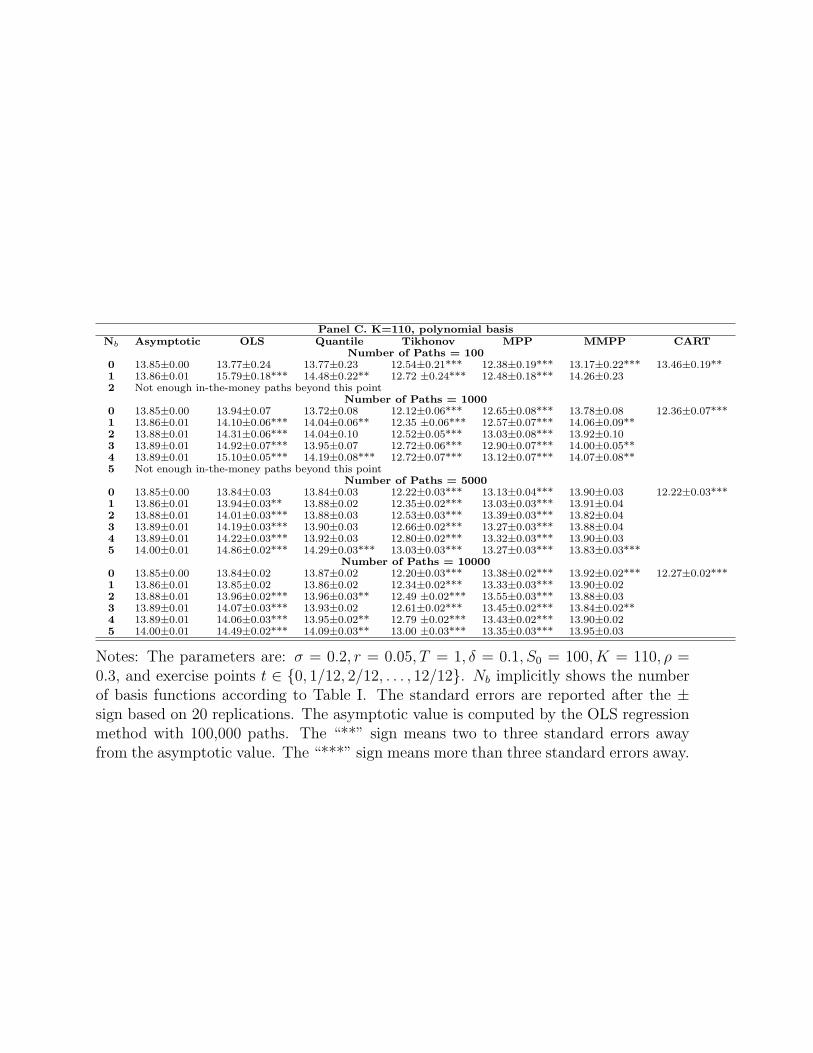
Panel C. K=110, polynomial basisNb Asymptotic OLS Quantile Tikhonov MPP MMPP CART

Number of Paths = 1000 13.85±0.00 13.77±0.24 13.77±0.23 12.54±0.21*** 12.38±0.19*** 13.17±0.22*** 13.46±0.19**1 13.86±0.01 15.79±0.18*** 14.48±0.22** 12.72 ±0.24*** 12.48±0.18*** 14.26±0.232 Not enough in-the-money paths beyond this point

Number of Paths = 10000 13.85±0.00 13.94±0.07 13.72±0.08 12.12±0.06*** 12.65±0.08*** 13.78±0.08 12.36±0.07***1 13.86±0.01 14.10±0.06*** 14.04±0.06** 12.35 ±0.06*** 12.57±0.07*** 14.06±0.09**2 13.88±0.01 14.31±0.06*** 14.04±0.10 12.52±0.05*** 13.03±0.08*** 13.92±0.103 13.89±0.01 14.92±0.07*** 13.95±0.07 12.72±0.06*** 12.90±0.07*** 14.00±0.05**4 13.89±0.01 15.10±0.05*** 14.19±0.08*** 12.72±0.07*** 13.12±0.07*** 14.07±0.08**5 Not enough in-the-money paths beyond this point

Number of Paths = 50000 13.85±0.00 13.84±0.03 13.84±0.03 12.22±0.03*** 13.13±0.04*** 13.90±0.03 12.22±0.03***1 13.86±0.01 13.94±0.03** 13.88±0.02 12.35±0.02*** 13.03±0.03*** 13.91±0.042 13.88±0.01 14.01±0.03*** 13.88±0.03 12.53±0.03*** 13.39±0.03*** 13.82±0.043 13.89±0.01 14.19±0.03*** 13.90±0.03 12.66±0.02*** 13.27±0.03*** 13.88±0.044 13.89±0.01 14.22±0.03*** 13.92±0.03 12.80±0.02*** 13.32±0.03*** 13.90±0.035 14.00±0.01 14.86±0.02*** 14.29±0.03*** 13.03±0.03*** 13.27±0.03*** 13.83±0.03***

Number of Paths = 100000 13.85±0.00 13.84±0.02 13.87±0.02 12.20±0.03*** 13.38±0.02*** 13.92±0.02*** 12.27±0.02***1 13.86±0.01 13.85±0.02 13.86±0.02 12.34±0.02*** 13.33±0.03*** 13.90±0.022 13.88±0.01 13.96±0.02*** 13.96±0.03** 12.49 ±0.02*** 13.55±0.03*** 13.88±0.033 13.89±0.01 14.07±0.03*** 13.93±0.02 12.61±0.02*** 13.45±0.02*** 13.84±0.02**4 13.89±0.01 14.06±0.03*** 13.95±0.02** 12.79 ±0.02*** 13.43±0.02*** 13.90±0.025 14.00±0.01 14.49±0.02*** 14.09±0.03** 13.00 ±0.03*** 13.35±0.03*** 13.95±0.03

Notes: The parameters are: σ = 0.2, r = 0.05, T = 1, δ = 0.1, S0 = 100, K = 110, ρ =0.3, and exercise points t ∈ {0, 1/12, 2/12, . . . , 12/12}. Nb implicitly shows the numberof basis functions according to Table I. The standard errors are reported after the ±sign based on 20 replications. The asymptotic value is computed by the OLS regressionmethod with 100,000 paths. The “**” sign means two to three standard errors awayfrom the asymptotic value. The “***” sign means more than three standard errors away.

Tab

leV

III:

Ove

rall

Per

form

ance

Com

par

ison

Cas

eO

LS

Quan

tile

Tik

hon

ovM

PP

MM

PP

CA

RT

Pan

elA

.Pol

ynom

ialbas

isC

ase

1–

o+

++

––

––

++

+o

++

+o

++

+–

–+

oC

ase

2–

o+

+o

––

–o

++

++

++

+o

++

+–

–+

–C

ase

3+

++

++

++

++

+o

–+

o–

–+

+–

o+

o–

–C

ase

4o

++

++

––

–+

++

++

+o

–+

++

+–

–+

–C

ase

5(n

=2,

K=

80)

––

o+

–+

––

–o

+o

o–

––

–o

oo

––

––

Cas

e5

(n=

2,K

=10

0)–

o+

++

o–

––

o+

++

––

–+

++

+o

––

–C

ase

5(n

=2,

K=

110)

––

o+

+–

––

o–

oo

+o

––

++

++

++

––

Cas

e5

(n=

3,K

=80

)–

–o

o–

o+

oo

––

–o

––

–o

oo

o+

––

–C

ase

5(n

=3,

K=

100)

––

oo

o+

o–

––

––

o–

––

++

o–

+–

––

Cas

e5

(n=

3,K

=11

0)–

–o

++

+–

–o

––

––

––

–+

+o

o+

––

–C

ase

5(n

=5,

K=

80)

––

–o

––

o+

o–

––

o–

––

–+

oo

––

––

Cas

e5

(n=

5,K

=10

0)–

–o

o–

o+

+–

––

–o

––

–o

++

o–

––

–C

ase

5(n

=5,

K=

110)

––

oo

++

+o

o–

––

––

––

++

+o

+–

––

Cas

e5

(n=

10,K

=80

)–

–o

oo

–o

oo

––

–o

––

–o

++

+–

––

–C

ase

5(n

=10

,K=

100)

––

oo

––

oo

––

––

––

––

o+

+o

––

––

Cas

e5

(n=

10,K

=11

0)o

o–

o+

++

+–

––

––

––

–o

++

+o

––

–Pan

elB

.Pol

ynom

ialan

dEuro

pea

npri

cebas

isC

ase

1–

–o

+–

––

––

++

+–

++

+–

++

+–

–+

–C

ase

2–

o+

+o

––

–o

++

++

++

++

++

+–

–+

+C

ase

3+

++

++

++

++

++

++

++

++

++

+o

––

–C

ase

4–

o+

+–

+–

–+

++

++

++

++

++

+–

–+

–C

ase

5(n

=2,

K=

80)

––

o–

––

––

–+

++

–+

++

–o

++

o–

––

Cas

e5

(n=

2,K

=10

0)–

––

o–

o–

––

++

+o

++

+–

++

++

––

–C

ase

5(n

=2,

K=

110)

––

–+

––

o+

++

++

o+

++

––

Not

es:

“+”

,“o

”,

and

“–”,

resp

ecti

vely

repre

sent

good,

neu

tral

,an

dpoor

per

form

ance

.T

he

four

colu

mns

for

each

met

hod

corr

espon

dto

the

resu

lts

wit

hdiff

eren

tnum

ber

sof

sim

ula

tion

pat

hs

(100

,1,

000,

5,00

0,an

d10

,000

sim

ula

tion

pat

hs

resp

ecti

vely

from

left

toth

eri

ght)

.For

case

5,n

isth

enum

ber

ofunder

lyin

gas

sets

and

Kis

the

stri

kepri

ce.

Som

ece

lls

hav

em

issi

ng

valu

esbec

ause

ofnot

enou

ghin

-the-

mon

eypat

hs

for

the

spec

ifica

tion

.

Tab

leIX

:Per

form

ance

Com

par

ison

wit

hth

eLar

gest

Num

ber

ofB

asis

Funct

ions

Cas

eO

LS

Quan

tile

Tik

hon

ovM

PP

MM

PP

CA

RT

Pan

elA

.Pol

ynom

ialbas

isC

ase

1−

−+

+o

−−

−−

++

+−

++

+o

++

o−

−+

oC

ase

2−

−+

+o

−−

−−

++

++

++

o+

++

+−

−+

−C

ase

3+

++

++

++

++

++

oo

o−

−+

+−

−+

o−

−C

ase

4−

++

o+

−−

−+

++

++

++

o+

++

o−

−+

−C

ase

5(n

=2,

K=

80)

−−

−+

−+

o−

−+

+−

+−

−−

−o

o−

−−

−−

Cas

e5

(n=

2,K

=10

0)−

−+

++

+−

−−

o+

o+

−−

−−

++

+o

−−

−C

ase

5(n

=2,

K=

110)

−−

−o

−−

oo

+o

−−

++

++

+−

−C

ase

5(n

=3,

K=

80)

−−

−−

−−

++

+−

−−

+−

−−

−o

−−

+−

−−

Cas

e5

(n=

3,K

=10

0)−

−−

−−

o+

++

−−

−+

−−

−o

oo

−+

−−

−C

ase

5(n

=3,

K=

110)

−−

−+

−−

−−

−−

−−

+o

o+

−−

−C

ase

5(n

=5,

K=

80)

−−

−−

−−

−+

+−

−−

o−

−−

−+

−−

−−

−−

Cas

e5

(n=

5,K

=10

0)−

−−

−−

−−

+−

−−

−+

−−

−−

++

+−

−−

−C

ase

5(n

=5,

K=

110)

−−

−−

++

−−

−−

−−

++

−+

−−

−C

ase

5(n

=10

,K=

80)

−−

−−

−−

−−

−−

−−

+−

−−

−−

−C

ase

5(n

=10

,K=

100)

−−

−−

−−

−−

−−

−−

++

−−

−−

−C

ase

5(n

=10

,K=

110)

−−

−o

−−

−−

−+

o−

−−

Pan

elB

.Pol

ynom

ialan

dEuro

pea

npri

cebas

isC

ase

1−

−−

+−

+−

−−

−+

+−

++

+o

−+

+−

−+

−C

ase

2−

−+

+−

−−

−−

++

++

++

++

++

+−

−+

+C

ase

3+

++

++

+−

++

++

++

++

++

++

+o

−−

−C

ase

4o

−+

+o

+−

−+

++

+o

o+

++

++

+−

−+

−C

ase

5(n

=2,

K=

80)

−−

+−

−−

−−

−+

++

−+

++

−−

++

o−

−−

Cas

e5

(n=

2,K

=10

0)−

−−

−−

o−

−−

++

+o

++

+−

o+

++

−−

−C

ase

5(n

=2,

K=

110)

−−

−−

−−

−+

oo

++

−+

++

−−

Not

es:

“+”

,“o

”,

and

“–”

,re

spec

tive

lyre

pre

sent

good

(wit

hin

two

stan

dar

der

rors

from

the

asym

pto

tic

valu

e),

neu

tral

(tw

oto

thre

est

andar

der

rors

away

from

the

asym

pto

tic

valu

e),

and

poor

(mor

eth

anth

ree

stan

dar

der

rors

away

)per

form

ance

.T

he

four

colu

mns

for

each

met

hod

corr

espon

dto

the

resu

lts

wit

hdiff

eren

tnum

ber

sof

sim

ula

tion

pat

hs

(100

,1,

000,

5,00

0,an

d10

,000

sim

ula

tion

pat

hs

resp

ecti

vely

from

left

toth

eri

ght)

.For

case

5,n

isth

enum

ber

ofunder

lyin

gas

sets

and

Kis

the

stri

kepri

ce.

Som

ece

lls

hav

em

issi

ng

valu

esbec

ause

ofnot

enou

ghin

-the-

mon

eypat

hs

for

the

spec

ifica

tion

.

Tab

leX

:Per

form

ance

Com

par

ison

ofC

ases

wit

hD

iffer

ent

Num

ber

sof

Exer

cise

Tim

esC

ase

OLS

Quan

tile

Tik

hon

ovM

PP

MM

PP

CA

RT

Pan

elA

.C

ase

23

exer

cise

tim

esP

o+

++

+–

––

++

++

++

++

++

++

––

+o

6ex

erci

seti

mes

P–

o+

+o

––

–o

++

++

++

+o

++

+–

–+

–3

exer

cise

tim

esP

and

E–

o+

+–

––

–+

++

++

++

++

++

++

–+

+6

exer

cise

tim

esP

and

E–

o+

+o

––

–o

++

++

++

++

++

+–

–+

+Pan

elB

.C

ase

5,n

=2,

K=

803

exer

cise

tim

esP

–+

++

++

+o

–+

o+

+o

oo

++

oo

––

––

6ex

erci

seti

mes

P–

o+

+o

o+

+–

o+

oo

oo

–o

+o

o+

––

–12

exer

cise

tim

esP

––

o+

–+

––

–o

+o

o–

––

–o

oo

––

––

3ex

erci

seti

mes

Pan

dE

–o

++

–+

o–

o+

++

++

++

++

++

o–

––

6ex

erci

seti

mes

Pan

dE

––

oo

–o

++

–+

++

–+

++

–+

++

––

––

12ex

erci

seti

mes

Pan

dE

––

o–

––

––

–+

++

–+

++

–o

++

o–

––

Pan

elC

.C

ase

5,n

=2,

K=

100

3ex

erci

seti

mes

Po

o+

++

––

–o

++

++

oo

o+

++

+–

o–

–6

exer

cise

tim

esP

––

++

++

––

–o

++

+o

––

++

++

––

––

12ex

erci

seti

mes

P–

o+

++

+–

––

o+

++

––

–+

++

+o

––

–3

exer

cise

tim

esP

and

E–

–o

+–

o–

–o

++

+o

++

+o

++

+o

––

–6

exer

cise

tim

esP

and

E–

–o

o–

+–

––

++

++

++

+–

++

+–

––

–12

exer

cise

tim

esP

and

E–

––

o–

o–

––

++

+o

++

+–

++

++

––

–Pan

elD

.C

ase

5,n

=2,

K=

110

3ex

erci

seti

mes

P–

++

+o

––

–o

o+

++

+o

o+

++

++

o–

–6

exer

cise

tim

esP

oo

++

+o

––

oo

++

++

––

++

++

++

––

12ex

erci

seti

mes

P–

–o

++

––

–o

–o

o+

o–

–+

++

++

+–

–3

exer

cise

tim

esP

and

E–

–+

+–

o–

–o

++

++

++

+o

++

++

+–

–6

exer

cise

tim

esP

and

E–

–+

+–

–+

++

++

++

++

––

–12

exer

cise

tim

esP

and

E–

––

+–

–o

++

++

+o

++

+–

–

Not

es:

“+”

,“o

”,an

d“–

”,re

spec

tive

lyre

pre

sent

good

(wit

hin

two

stan

dar

der

rors

from

the

asym

pto

tic

valu

e),neu

tral

(tw

oto

thre

est

andar

der

rors

away

from

the

asym

pto

tic

valu

e),

and

poor

(mor

eth

anth

ree

stan

dar

der

rors

away

)per

form

ance

.“P

”re

pre

sents

pol

ynom

ial

bas

is.

“Pan

dE

”re

pre

sents

the

bas

isw

ith

bot

hpol

ynom

ials

and

Euro

pea

nop

tion

pri

ces.

The

four

colu

mns

for

each

met

hod

corr

espon

dto

the

resu

lts

wit

hdiff

eren

tnum

ber

sof

sim

ula

tion

pat

hs

(100

,1,

000,

5,00

0,an

d10

,000

sim

ula

tion

pat

hs

resp

ecti

vely

from

left

toth

eri

ght)

.For

case

5,n

isth

enum

ber

ofunder

lyin

gas

sets

and

Kis

the

stri

kepri

ce.

Som

ece

lls

hav

em

issi

ng

valu

esbec

ause

ofnot

enou

ghin

-the-

mon

eypat

hs

for

the

spec

ifica

tion

.