Regression-Based Monte Carlo For Pricing High-Dimensional ...

Regression-Based Monte Carlo For PricingHigh-Dimensional American-Style Options

Niklas [email protected]

Umea UniversityDepartment of Physics

April 7, 2016

Master’s Thesis in Engineering Physics, 30 hp.Supervisor: Oskar Janson ([email protected])

Examiner: Markus Adahl ([email protected])

Abstract

Pricing different financial derivatives is an essential part of the financial industry. Forsome derivatives there exists a closed form solution, however the pricing of high-dimensionalAmerican-style derivatives is still today a challenging problem. This project focuses on thederivative called option and especially pricing of American-style basket options, i.e. optionswith both an early exercise feature and multiple underlying assets. In high-dimensional prob-lems, which is definitely the case for American-style options, Monte Carlo methods is advan-tageous. Therefore, in this thesis, regression-based Monte Carlo has been used to determineearly exercise strategies for the option. The well known Least Squares Monte Carlo (LSM)algorithm of Longstaff and Schwartz (2001) has been implemented and compared to RobustRegression Monte Carlo (RRM) by C.Jonen (2011). The difference between these methodsis that robust regression is used instead of least square regression to calculate continuationvalues of American style options. Since robust regression is more stable against outliers theresult using this approach is claimed by C.Jonen to give better estimations of the option price.

It was hard to compare the techniques without the duality approach of Andersen andBroadie (2004) therefore this method was added. The numerical tests then indicate that theexercise strategy determined using RRM produces a higher lower bound and a tighter upperbound compared to LSM. The difference between upper and lower bound could be up to 4times smaller using RRM.

Importance sampling and Quasi Monte Carlo have also been used to reduce the variancein the estimation of the option price and to speed up the convergence rate.

1

Sammanfattning

Prissattning av olika finansiella derivat ar en viktig del av den finansiella sektorn. For vissaderivat existerar en sluten losning, men prissattningen av derivat med hog dimensionalitet ochav amerikansk stil ar fortfarande ett utmanande problem. Detta projekt fokuserar pa derivatetsom kallas option och sarskilt prissattningen av amerikanska korg optioner, dvs optioner sombade kan avslutas i fortid och som bygger pa flera underliggande tillgangar. For problemmed hog dimensionalitet, vilket definitivt ar fallet for optioner av amerikansk stil, ar MonteCarlo metoder fordelaktiga. I detta examensarbete har darfor regressions baserad Monte Carloanvants for att bestamma avslutningsstrategier for optionen. Den valkanda minsta kvadratMonte Carlo (LSM) algoritmen av Longstaff och Schwartz (2001) har implementerats ochjamforts med Robust Regression Monte Carlo (RRM) av C.Jonen (2011). Skillnaden mellanmetoderna ar att robust regression anvands istallet for minsta kvadratmetoden for att beraknafortsattningsvarden for optioner av amerikansk stil. Eftersom robust regression ar mer stabilmot avvikande varden pastar C.Jonen att denna metod ger battre skattingar av optionspriset.

Det var svart att jamfora teknikerna utan tillvagagangssattet med dualitet av Andersenoch Broadie (2004) darfor lades denna metod till. De numeriska testerna indikerar da attavslutningsstrategin som bestamts med RRM producerar en hogre undre grans och en snavareovre grans jamfort med LSM. Skillnaden mellan ovre och undre gransen kunde vara upp till4 ganger mindre med RRM.

Importance sampling och Quasi Monte Carlo har ocksa anvants for att reducera varianseni skattningen av optionspriset och for att paskynda konvergenshastigheten.

2

Niklas Andersson April 7, 2016

Contents

1 Introduction 5

1.1 Options . . . . . . . . . . . . . . . . . . . . . . . . . . . . . . . . . . . . . . . . . . 5

1.2 Pricing Options . . . . . . . . . . . . . . . . . . . . . . . . . . . . . . . . . . . . . . 6

2 Theory 7

2.1 Monte Carlo . . . . . . . . . . . . . . . . . . . . . . . . . . . . . . . . . . . . . . . . 7

2.1.1 Kolmogorov’s strong law of large numbers . . . . . . . . . . . . . . . . . . . 7

2.1.2 Monte Carlo simulation . . . . . . . . . . . . . . . . . . . . . . . . . . . . . 7

2.1.3 Central Limit Theorem . . . . . . . . . . . . . . . . . . . . . . . . . . . . . 8

2.1.4 Error estimation . . . . . . . . . . . . . . . . . . . . . . . . . . . . . . . . . 8

2.1.5 Advantages of Monte Carlo . . . . . . . . . . . . . . . . . . . . . . . . . . . 9

2.2 Dynamics of the stock price . . . . . . . . . . . . . . . . . . . . . . . . . . . . . . . 9

2.3 Monte Carlo for pricing financial derivatives . . . . . . . . . . . . . . . . . . . . . . 10

2.4 Robust Regression . . . . . . . . . . . . . . . . . . . . . . . . . . . . . . . . . . . . 13

2.5 Duality approach . . . . . . . . . . . . . . . . . . . . . . . . . . . . . . . . . . . . . 14

2.6 Variance reduction . . . . . . . . . . . . . . . . . . . . . . . . . . . . . . . . . . . . 15

2.6.1 Importance sampling . . . . . . . . . . . . . . . . . . . . . . . . . . . . . . . 16

2.6.2 Importance sampling in finance . . . . . . . . . . . . . . . . . . . . . . . . . 16

2.7 Quasi Monte Carlo . . . . . . . . . . . . . . . . . . . . . . . . . . . . . . . . . . . . 18

2.7.1 Discrepancy and error estimation . . . . . . . . . . . . . . . . . . . . . . . . 18

2.7.2 Sobol sequence . . . . . . . . . . . . . . . . . . . . . . . . . . . . . . . . . . 19

2.7.3 Dimensionality Reduction . . . . . . . . . . . . . . . . . . . . . . . . . . . . 20

3 Method 21

3.1 Algorithms . . . . . . . . . . . . . . . . . . . . . . . . . . . . . . . . . . . . . . . . 22

3.1.1 LSM and RRM . . . . . . . . . . . . . . . . . . . . . . . . . . . . . . . . . . 22

3


3.1.2 Duality approach . . . . . . . . . . . . . . . . . . . . . . . . . . . . . . . . . 23

4 Results 24

4.1 LSM vs RRM . . . . . . . . . . . . . . . . . . . . . . . . . . . . . . . . . . . . . . . 24

4.1.1 Duality approach . . . . . . . . . . . . . . . . . . . . . . . . . . . . . . . . . 29

4.2 Quasi MC . . . . . . . . . . . . . . . . . . . . . . . . . . . . . . . . . . . . . . . . . 31

4.3 Importance Sampling . . . . . . . . . . . . . . . . . . . . . . . . . . . . . . . . . . . 34

4.4 Combinations . . . . . . . . . . . . . . . . . . . . . . . . . . . . . . . . . . . . . . . 36

5 Discussion 37

6 Appendix A1 39

6.1 Importance sampling example . . . . . . . . . . . . . . . . . . . . . . . . . . . . . . 39

6.2 Not only in-the-money paths . . . . . . . . . . . . . . . . . . . . . . . . . . . . . . 40

7 References 40

4


1 Introduction

After the financial crisis that started in 2007, the derivatives markets have been much criticized andmany governments have introduced rules requiring some over-the-counter (OTC) derivatives to becleared by clearing houses[1]. This thesis has been performed at Cinnober Financial Technology.Cinnober is an independent supplier of financial technology to marketplaces and clearinghouses.When more and more complex derivatives are brought to the market the requirements of theclearing houses to clear and evaluate them increases. Therefore, the pricing of different derivativesis an important part of the financial industry today. A financial derivative is a financial instrumentthat is built upon a more basic underlying variable like a bond, interest rate or stock. This projectfocuses on the derivative called option and specifically the pricing of American-style multi-assetoptions using regression-based Monte Carlo methods.

1.1 Options

There are two different kinds of options, call options and put options. Buying a call option meansbuying a contract that gives the right to buy the underlying asset at a specified date, expirationdate T, for a specified price, strike price K. This is also referred to as taking a long position in acall option and for this you pay a premium. If one instead takes a short position in a call optionyou have the obligation to sell the underlying asset at the expiration date T for the strike priceK and for this obligation you receive the premium. On the other hand, a long position in a putoption gives the right to sell the underlying asset whereas the short position has the obligation tobuy the underlying asset, see Table 1.

Table 1: Explanation of the states Long/Short in a Call/Put option.

CallLong: Gives the right to buy the underlying asset.

↓ premium

Short: Obligation to sell if long position choose to exercise.

PutLong: Gives the right to sell the underlying asset.

↓ premium

Short: Obligation to buy if long position choose to exercise.

The difference between an option and future/forward contracts is that the holder of a option hasthe right, but not the obligation, to do something whereas the holder of a future/forward contractis bound by the contract. Let’s take a call option to buy a stock S(t) with strike prize K andexpiration date T as an example. If the stock price S(T ) exceeds the strike price K in the futuretime T > t the holder can exercise the option with a profit of S(T )−K. If instead the stock priceS(T ) is less or equal to the strike price K the option is worthless for the holder. The payoff of acall option, C with strike price K and expiration date T , is thus,

C(S(T ),K, T ) = max0, S(T )−K. (1)

Options that only can be exercised at the expiration date T are called European options and optionsthat can be exercised at any time are called American options. There are also options whose valuedepend not only on the value of the underlying asset at expiration but on the whole path of theasset. The barrier option is an example of this kind of option. It either becomes active or stopbeing active if the underlying asset hits a pre-determined barrier during the lifetime of the option.A knock- in barrier option becomes active only if the barrier is crossed and knock-out barrier optionpays nothing if the barrier is crossed. The payoff of a down-and-in barrier call option with strike

5


price K, maturity date T and barrier H is,

C(S(T ),K,H, T ) = 1S(t)≤H ·max0, S(T )−K, (2)

where 1S(t)≤H is 1 if S(t) ≤ H at any time in the interval t=[0,T] and 0 otherwise.

There are also options on multiple underlying assets, these are called basket options. The payoffof a basket option is typically a function of either the maximum, minimum, arithmetic average orgeometric average of the assets prices, see Table 2.

Table 2: Different payoffs of multi-asset Call and Put options with strike price K and D numberof assets.

Type Call Put

Maximum: max0,max(s1, ..., sD)−K max0,K −max(s1, ..., sD)Minimum: max0,min(s1, ..., sD)−K max0,K −min(s1, ..., sD)Geometric average: max0, (

∏Di=1 si)

1/D −K max0,K − (∏Di=1 si)

1/DArithmetic average: max0, (

∑Di=1 si)/D −K max0,K − (

∑Di=1 si)/D

1.2 Pricing Options

Pricing European options is often done using the well known Black-Scholes-Merton model. Thismodel has had a big influence of the financial market since it provides a theoretic price for Europeanoptions. The importance of the model was recognized in 1997 when the inventors where awardedwith the Nobel prize in economics. Pricing American options is harder than pricing Europeanoptions, in fact the pricing and optimal exercise of options with early exercise features is one of themost challenging problems in mathematical finance[12]. Before you can value this kind of optionyou need to determine when the option will be exercised. There has been a lot of research in thisarea trying to determine the optimal stopping strategy and it is one topic that this project willfocus on. Regression-based Monte Carlo techniques for determining optimal stopping strategieshad a breakthrough with the proposal of Longstaff and Schwartz in 2001 [3]. In their method leastsquare regression is used to determine exercise dates. C. Jonen published his dissertation in 2011where he instead suggests using robust regression in the regression step. This project will focus oncomparing the least square method by Longstaff and Schwartz, and the robust regression methodby C. Jonen [4].

As mentioned there is no analytic formula for pricing an American option so one instead turnsto numerical methods, like the binomial model or the finite difference method to solve the partialstochastic differential equation describing the price process of the option. These methods workvery good for options that have only one underlying asset but if the option is a multi-asset optionwith two or more underlying assets these methods lose their strength. Another approach to priceoptions are Monte Carlo methods and this is the approach that will be used in this project. Insteadof finding a solution of the price numerically we simulate the path of the underlying assets using astochastic representation and valuate the option from this path. We repeat this procedure manytimes, calculate the average of all these simulations and use this as an estimate of the option price.

An advantage of Monte Carlo is that it is a relatively easy procedure which can be applied toprice various kinds of derivatives. The disadvantage is that it is a computational costly methodsince stochastic paths have to be calculated which implies a slow convergence rate. However theconvergence rate O( 1√

n) holds for all dimensions in contrast to numerical methods where the con-

vergence rate decreases with the number of dimensions. American-style basket options incorporate

6


two sources of high-dimensionality, the underlying stocks and time to maturity. Therefore, MonteCarlo methods are often the method of choice when pricing American-style basket options[2].

For the most part there is nothing or very little that can be done about the rather slow convergencerate of Monte Carlo, under appropriate conditions quasi Monte Carlo is an exception. We can,however, look for better sampling techniques and variance reduction methods to reduce the variancein the estimation. There are many different types of variance reduction techniques, antitheticvariates, control variates, importance sampling, stratified sampling and quasi Monte Carlo aresome well known techniques. Depending on the type of option it may vary which method is thebest. In this project the use of importance sampling will be examined, this is a more complexmethod and require some knowledge of the underlying problem but it has the capacity to produceorders of magnitude variance reduction. The effect of quasi Monte Carlo will also be studied.

2 Theory

Before I explain how to use Monte Carlo for financial applications I will start this section by givingthe basic theory for Monte Carlo methods in general, this is handled in subsection 2.1. Subsection2.2 and 2.3 will be about how to model stock prices and how to use regression-based Monte Carloto determine exercise dates for options. The basic idea of robust regression and the extension toduality methods is explained in subsection 2.4 and 2.5 and I will end this section with some theoryof importance sampling and quasi Monte Carlo.

2.1 Monte Carlo

2.1.1 Kolmogorov’s strong law of large numbers

This law is the main justification of the Monte Carlo methods and state that the average of asequence of iid, i.e. independent identically distributed, variates will converge almost surely to theexpected value. Given a sequence of iid variates ζi with expectation

E[ζi] = µ, (3)

define the average as

X =1

N

N∑i=1

ζi. (4)

Then this average will converge almost surely to µ,

Xa.s.−−→ µ, when N →∞. (5)

2.1.2 Monte Carlo simulation

Let’s consider the following integral,

θ =

∫ 1

0

f(x)dx = [F (x)]10. (6)

7


If the function f(x) is a complicated function and it is hard to find the primitive function F (x)

we can instead use Monte Carlo to approximate the integral with θN = 1N

∑Ni=1 f(Ui), where

Ui ∼ U(0, 1) are random uniform variables with density,

gU (x) =

1 0 ≤ x ≤ 10 Otherwise.

(7)

To understand that θN is a estimator of θ lets first show that the expectation of E[f(U)] =∫ 1

0f(x)dx.

E[f(U)] =

∫Rf(x)gU (x)dx =

∫ 0

−∞f(x)gU (x)dx+

∫ 1

0

f(x)gU (x)dx+

∫ ∞1

f(x)gU (x)dx =∫ 0

−∞f(x) · 0dx+

∫ 1

0

f(x) · 1dx+

∫ ∞1

f(x) · 0dx =

∫ 1

0

f(x)dx.

(8)

The next step is to use the Kolmogorov’s strong law of large numbers

θN = 1N

∑Ni=1 f(Ui)

a.s.−−→ E[f(U)] = θ as N →∞. (9)

Hence, by simulating U1, U2, ..., UN , evaluating the function at these points and averaging we getan unbiased estimator of θ.

2.1.3 Central Limit Theorem

Let ζ1, ζ2,..., ζN be iid. random variables with E[ζi] = µ and V ar[ζi] = σ2 <∞, then the composite

variable XN =1N

∑Ni=1 ζi−µσ/√N

converges in distribution to the standard normal as N increases,

XN =1N

∑Ni=1 ζi−µσ/√N

i.d.−−→ N (0, 1) as N →∞. (10)

2.1.4 Error estimation

Given the Monte Carlo estimation in (9) the central limit theorem gives

θN−θσ/√N

i.d.−−→ N (0, 1) as N →∞ (11)

where σ is the standard deviation of θN . Since σ is unknown we have to approximate it with s,

s =

√√√√ 1

N − 1

N∑i=1

(f(Ui)− θN )2. (12)

By inserting s instead of σ in (11) we see that θNi.d.−−→ N (θ, s

2

N ) this leads to the definition of the

standard error, SE which is a measure of the deviation in θN .

SE =

√V ar(θN ) =

s√N. (13)

We can now create a 100(1− α)% confidence interval for the estimator θN as[θN − z1−α/2 · SE; θN + z1−α/2 · SE

](14)

where z1−α/2 denotes the (1− α/2) quantile of the normal distribution and z1−0.05/2 ≈ 1.96 for a95% confidence interval.

8


2.1.5 Advantages of Monte Carlo

The integral in (6) can also be calculated numerically using for example the trapezoidal rule,

θt.rN =f(0) + f(1)

2N+

1

N

N−1∑i=1

f(i/N). (15)

The error from using trapezoidal rule is of order O(N−2) which is better than the Monte Carloestimate, O(N−1/2), so how come we use Monte Carlo? The strength of Monte Carlo is that itis of order O(N−1/2) regardless of the dimensionality of the problem, whereas the error for thetrapezoidal rule is of order O(N−2/d). This degradation in convergence rate as the dimension ofthe problem increase are common for all deterministic integration methods[2]. Hence, Monte Carlomethods are superior for evaluating integrals in higher dimensions.

2.2 Dynamics of the stock price

In order to use Monte Carlo methods to price options we need to generate paths of the underlyingasset, thus stocks. One common assumption in financial applications is that the evolution of thestock price can be represented by a stochastic process, and especially the geometric Brownianmotion under the risk neutral valuation,

dS(t)

S(t)= (r − δ)dt+ σdW (t) (16)

where, r is the risk-free interest rate, δ the yearly dividend yield, σ the volatility and W is aBrownian motion. A standard Brownian Motion (or a Wiener process) is defined by the followingconditions,

1. W (0) = 0.

2. The process W has independent increments, i.e. if r < s < t < u then W (u) −W (t) andW (s)−W (r) are independent stochastic variables.

3. For s < t the stochastic variable W (t)−W (s) has a Gaussian distribution N(0,√t− s) .

4. W has continuous trajectories.

The solution of (16) above is given by,

S(tl+1) = S(tl)e(r−δ− 1

2σ2)∆t+σ∆W , (17)

and due to the conditions 2 and 3 of the Brownian Motion, it possible to simulate the value of astock at discrete time steps, l = 0, ...L− 1 as

S(tl+1) = S(tl)e(r−δ− 1

2σ2)∆t+σZ(l+1), (18)

where Z(1), Z(2),... are N(0,√

∆t). For derivation of equations (16) and (17), I recommend thebook ”Arbitrage Theory in Continuous Time” by Tomas Bjork[13].

To generate paths of multiple assets the multidimensional Geometric Brownian Motion is used

dSi(t)Si(t)

= (r − δi)dt+ σidXi(t), i = 1, ..., d (19)

9


where r is the risk-free interest rate, δi and σi is the yearly dividend yield and the volatility of theith asset Si. X is the d-dimensional Brownian motion with covariance matrix Σi,j = ρi,jσiσj . Inthe multidimensional Brownian motion the increments are multivariate normally distributed withcovariance matrix Σ, X(t)−X(s) ∼ N(~0,

√t− s Σ). Hence, the following equation can be used for

generating paths of multiple assets

Si(tl+1) = Si(tl)e(r−δi− 1

2σ2i )∆t+

√∆t

∑dj=1 AijZl+1,j , i = 1, ..., d (20)

where Zl = (Zl1, ..., Zld) ∼ N(0,1d) and A is chosen to be the Cholesky factor of the covariancematrix Σ, satisfying AAT = Σ.

For more information and algorithms on how to model dependencies between variables I refer toGlasserman [2] or Jackel [5].

2.3 Monte Carlo for pricing financial derivatives

In the world of finance there is a big need of calculating expectations and determine future valuesof different derivatives. The underlying processes are often simulated using stochastic differentialsand it is common that if the expectations are written as integrals the dimensions are very large.Depending on the problem the dimensionality is often at least as large as the number of time steps.The strength of Monte Carlo is that it is a very attractive method for solving problems with highdimensionality and therefore the method is widely used in financial engineering.

To price a financial derivative by Monte Carlo one usually follows these steps,

• Simulate paths of the underlying assets.

• Evaluate the discounted payoffs from the simulated paths.

• Use the average of these discounted payoffs as an estimate of the derivative price.

However, the early exercise feature of an American-style option makes valuation harder and beforewe can price an American-style option we need a way to determine when the option will beexercised. When using Monte Carlo we simulate paths of the underlying asset as described insection 2.2 and use these to valuate the option, hence it may seem as an easy problem to determinewhen the option should be exercised. However, using knowledge of the asset paths and exercising atthe optimum is referred to as perfect forecast and tend to overestimate the option price. To betterestimate the exercise time one can use parametric approximation to determine exercise regionsbefore the simulation. But in higher dimensional problems the optimal exercise regions can behard to approximate using this technique [2, P.427].

Another approach to estimate the value of American options is by regression-based Monte Carlomethods. At each exercise time the holder of the option compares the value of exercising theoption immediately with the expected payoff of continuation. The value of exercising the optionimmediately at time t is called the intrinsic value whereas the expected payoff of holding on tothe option is called continuation value. The key insight in regression-based Monte Carlo methodsis that the continuation value can be estimated using regression. Before I go on and describe themethod, let’s begin with some assumptions[4].

• (Ω,F , P ) is a complete probability space, where the time horizon [0,T] is finite and F =Ft|0 ≤ t ≤ T is the filtration with the σ -Algebra Ft at time date t.

10


• There are no arbitrage opportunities in the market and the market is complete. This impliesexistence of a unique martingale measure P , which is equivalent to P .

• Bt denotes the value at time t of 1 money unit invested in a riskless money market accountat time date t = 0, i.e. Bt is described by

dBt = rtBtdt,B0 = 1,

where rt is the risk free interest rate at time t. Then, Ds,t denotes the discount factor givenby

Ds,t = Bs/Bt, s, t ∈ [0, T ].

In the special case of a constant risk-free rate r, we have

Bt = ert and Ds,t = e−r(t−s).

Furthermore we let the underlying asset S(t), 0 ≤ t ≤ T be a Markov processes that contains allnecessary information about the asset price and we restrict ourselves to the valuation of Bermudanoptions, i.e. options that only can be exercised at a fixed set of exercise opportunities, t1 < t2 <· · · < tL and denote Sl the state of the Markov process at time step l. In the following theconditional expectation given the Markov process up until time step l is denoted El[·] = E[·|Stl ].A fair price of an Bermudan option at time t0 is then given by the optimal stopping problem

supτ∈τ0,L

E0[D0,τZτ ], (21)

where τ0,L is the set of all stopping times with values in 0,...,L and (Zl)0≤l≤L is an adaptedpayoff process. Arbitrage reasoning justifies calling this a fair price for the option[2]. If we letVl(s) denote the value of the option at tl given Sl = s we are interested in the value V0(S0) whichmay be determined recursively as follows

VL = ZL

Vl = max(Zl, El[Dl,l+1Vl+1]), l = L− 1, ..., 0.(22)

This is the dynamic programming principle (DPP) in terms of the value process Vl which is anatural ansatz to solve the optimal stopping problem in (21). We start at the last time stepbecause we know that the value of the American option at this time step will equal the value ofthe European option which can be determined.

The dynamic programming recursions (22) focus on the option value, but sometimes it is moreconvenient to work with the optimal stopping time instead.

τ∗L = L

τ∗l =

l , Zl ≥ El[Dl,τ∗

l+1Zτ∗

l+1]

, l = L− 1, ..., 0.τ∗l+1 , otherwise

(23)

Following the DPP and using a set of N simulated paths Snln=1,...,N,l=0,...,L, the value at eachexercise date for each path can be determined by

V nL = ZnL

V nl = max(Znl , Cl(Snl)), l = L− 1, ..., 0(24)

where Cl(s) denotes the continuation value in state s and at time step l

Cl(s) = El[Dl,l+1Vl+1(Sl+1)], (25)

11


for l = 0, ..., L − 1. The idea of regression-based Monte Carlo methods is to estimate a modelfunction for the continuation value via regression. A model function for the continuation value Clat time step l is given by a linear combination of M basis functions φ(·), i.e.

Cl(s) =

M∑m=1

βmφm(s) (26)

where the coefficients βm might be determined by solving the least square problem,

minβ∈RM

||Cl − Cl||22. (27)

Numerically the problem in (27) can be solved by

minβ∈RM

1

N

N∑n=1

(Cnl − Cl(Snl))2, (28)

where N is the number of paths, and for n = 1, ..., N we have Cl(Snl) =∑Mm=1 βmφm(Snl) and Cnl

are the realizations of the continuation value of each path n,

Cnl = e−r∆tV nl+1 = e−r∆tmaxZnl+1, Cl+1(Sn,l+1), (29)

where Znl is the payoff at time step l of path n. Following this procedure gives an approximationof the option price today, i.e.

V0 = maxZ0, e−r∆t 1

N

N∑n=1

V n1 . (30)

To estimate option prices through (30) has however shown to give poor estimations and a break-through for regression-based Monte Carlo came with the least square Monte Carlo (LSM) technique,proposed by Longstaff and Schwartz in 2001, [3]. They work with the DPP in terms of the optimalstopping time as in (23), and hence try to determine the optimal stopping time for each simulatedpath by

τnL = L

τnl =

l , Zl(Snl) ≥ Cl(Snl)

, l = L− 1, ..., 1τnl+1 , otherwise

(31)

where the dependent variable Cnl , in the regression step is determined by

Cnl = e−r(τnl+1−l)∆tZτnl+1

, n = 1, ..., N, l = 1, ..., L (32)

instead as in (29). Once the optimal stopping time for each path has been determined the optionvalue can be estimated

V0 = maxZ0,1

N

N∑n=1

e−rτn1 ∆tZnτn1 . (33)

To evaluate V0 above one can either use the same set of paths that determined the stoppingstrategy or one might simulate a new set of paths and exercising according to the determinedexercise strategy. Longstaff and Schwartz recommend using only in-the-money paths in estimatingcontinuation value, i.e. only paths that can be exercised with a profit will be considered in theregression step.

12


2.4 Robust Regression

The idea of robust regression is to take outliers into account once calculating the continuationvalue in the least square Monte Carlo approach. Therefore the minimization problem in (28) isreplaced with

minβ∈RM

1

N

N∑n=1

`(Cnl − Cl(Snl)) (34)

where ` is a suitable loss function. Thus in order to implement the robust regression techniquein an already running LSM system we only replace the solver for regression. In the following theresiduals rnl will be denoted

rnl = Cnl − Cl(Snl) , l = 1, ..., L− 1, n = 1, ..., N.

The loss functions that will be used in this project are, ordinary least square OLS, Huber andJonen’s loss functions, see Table 3. To get an intuition of the properties for these loss functionsFigure 1 show their graphs.

Table 3: Different loss functions `(·) for robust regression.

`(r)

OLS r2

Huber

r2 , |r| ≤ γ1

2γ1|r| − γ21 , |r| > γ1

Jonen

r2 , |r| ≤ γ1

2γ1|r| − γ21 , γ1 < |r| < γ2

2γ1γ2 − γ21 , |r| ≥ γ2

Figure 1: Illustration of the different loss functions for robust regression, γ1 and γ2 are transitionpoints.

13


The idea of robust regression is to get a better approximation of the continuation value by givingoutliers less weight in the regression step. Outliers occur by strongly fluctuated paths and thedetermination of outliers is not trivial[4, P.21]. The transition points γ1 and γ2 determine whichpoints are considered outliers and not. The outlier detection procedure recommended by C.Jonenis the following,

rhelpn = |rn|, n = 1, ..., N, r = (r1, ..., rN )

rhelp = sort(rhelp)

γ1 = rhelpbαNc, 0 << α < 1

γ2 = rhelpbβNc, α < β < 1.

(35)

The assumption is hence that (1 − α)100 percent of the data points are outliers. The reasonthat this empirical α-quantiles procedure is suggested is because we are not familiar with anydistribution of the error[4].

2.5 Duality approach

Andersen and Broadie introduced their Primal-Dual Simulation Algorithm in 2004 [9] which todayis a valuable extension to regression based Monte Carlo methods. Their method combined with theLSM method of Longstaff and Schwartz [3] is often the method of choice and implemented in manyoption pricing systems of financial institutions today[4]. Following the strategy of Longstaff andSchwartz as in (31) usually produces a low estimator of the option price. This is due to that thevalue of the option V0 is given by the supremum in (21) which is achieved by an optimal stoppingtime τ∗ hence following the procedure in (31) produces a low estimation of the option price

L0 := E0[D0,τZτ ] ≤ V0 = supτ∈τ0,L

E0[D0,τZτ ]. (36)

The idea of Andersen and Broadie’s approach is to create a high estimation to constrict the fairoption price V0 between the low and high estimation.

A consequence of the DPP (22) is that

Vl ≥ El[Dl,l+1Vl+1(Sl+1)], (37)

for all l=0,...,L-1. This is the defining property of a supermartingale. For more theory on martin-gales I refer to [13]. Due to (37) we can derive a dual problem for pricing options with an earlyexercise feature as follows[4]

LetH1 be the space of martingales M = (Ml)0≤l≤L for which sup0≤l≤L |Ml| ∈ Lp where Lp denotesthe space of all random variables with finite p-th moment, p ≥ 1. For any martingale M ∈ H1, wehave

supτ∈τ 1,L

E0[D0,τZτ ] = supτ∈τ 1,L

E0[D0,τZτ −Mτ +Mτ ]

= supτ∈τ 1,L

E0[D0,τZτ −Mτ ] +M0

≤ E0[ maxl=1,..L

(D0,lZl −Ml)] +M0,

(38)

14


where the second equality follows from the martingale property and the optional sampling theorem.As the upper bound holds for any martingale M , the option value might be estimated by

supτ∈τ 1,L

E0[D0,τZτ ] ≤ infM∈H1

(E0[ maxl=1,..L

(D0,lZl −Ml)]+M0). (39)

The right hand side of (39) is called a dual problem for pricing options with a early exercise feature.One can show that (39) holds with equality if the optimal martingale is found, to show this onemay consider the Doob-Meyer decomposition of the supermartingale (D0,lVl)0≤l≤L see Rogers [14].Finding the optimal martingale appears to be as difficult as solving the original stopping problem,but if we can find a martingale M that is close to the optimal martingale we can use

E0[ maxl=1,..L

(D0,lZl − Ml)]+ M0 (40)

to estimate an upper bound for the option price. A suboptimal exercise policy provides a lowerbound and by extracting a martingale from this suboptimal policy the dual value complements thelower bound with an upper bound. Thus the strategy becomes [4]

1. Find a stopping policy τ with values in 1,...,L and a martingale M that are optimal in thesense that they are good approximations to the optimal stopping times τ∗1 and the optimalmartingales M∗, respectively.

2. Calculate a lower bound L0 and an upper bound U0 for the fair value of an American-styleoption by

L0 := E0[D0,τZτ ] ≤ supτ∈τ 1,L

E0[D0,τZτ ] ≤ E0[ maxl=1,...,L

(D0,lZl − Ml)]+ M0 =: U0. (41)

The algorithm for this approach and an example of how to find a martingale is described in thesection 3.1.2. When pricing high dimensional options it is often hard to calculate any benchmarksvalues, therefore the method of Andersen and Broadie is often implemented so that we are not inthe dark with our calculations. Another reason for using this method is that the difference betweenthe lower and upper bound can be seen as a measure of how good we have estimated the optimalstopping time. The less difference the better estimate of the optimal stopping time. Therefore wecan use this method to compare and evaluate the least square Monte Carlo (LSM) with the robustregression Monte Carlo (RRM).

2.6 Variance reduction

Let θ be the parameter of interest, such that θ = E(X) where we can simulate X1, X2, ...XN

and use the average of these as an estimator θN of θ. Then to make θN a good estimator we

need the standard error SE =

√var(θN )/N , to be small. This can be done by increasing the

number of samples, N , but we notice that in order to increase the precision by a factor 2 we needto increase the number of samples by a factor of 4. Another strategy is to work with differentvariance reduction techniques. We cannot decrease V ar(θN ) but we can find another variableY such that E[Y ] = E[X] but V ar[Y ] < V ar[X]. There are many different variance reductiontechniques that can be used, antithetic variables, control variates, stratified sampling to mentionsome. The method that will be examined and used in this project is importance sampling whichis a more complex method and requires some knowledge of the particular problem but it has thecapacity to reduce the variance significantly.

15


2.6.1 Importance sampling

The standard Monte Carlo approach will have problem estimating θ = Ef (h(X)) =∫h(x)f(x)dx

if it is very unlikely that h(x) is obtained under the probability function f(x), i.e. only in veryrare cases we observe h(x). If we instead can find a probability function g(x) that makes it morelikely that we obtain h(x) we can observe that,

θ = Ef (h(X)) =

∫h(x)f(x)dx =

∫h(x)f(x)

g(x)g(x)dx = Eg(

h(x)f(x)

g(x)).

Hence we can write

θ = Eg(h(x)f(x)

g(x)),

where x has the new density g instead of f . So instead of using θ = 1N

N∑i=1

h(Xi), where Xi

are sampled from density f(x) we can use θIS = 1N

N∑i=1

h(Xi)f(Xi)g(Xi)

as our estimator where Xi are

sampled under g(x). The weight f(Xi)/g(Xi) is called the likelihood ratio and we should try tofind g(x) ∝ h(x)f(x) to obtain large variance reduction using this technique.

In order to select a proper density g, the exponentially tilted distribution density is often used,

g(x) = ft(x) =etxf(x)

M(t), (42)

where −∞ < t < ∞ and M(t) is the moment generating function M(t) = E[etx]. See Appendixfor an example of how to use importance sampling.

2.6.2 Importance sampling in finance

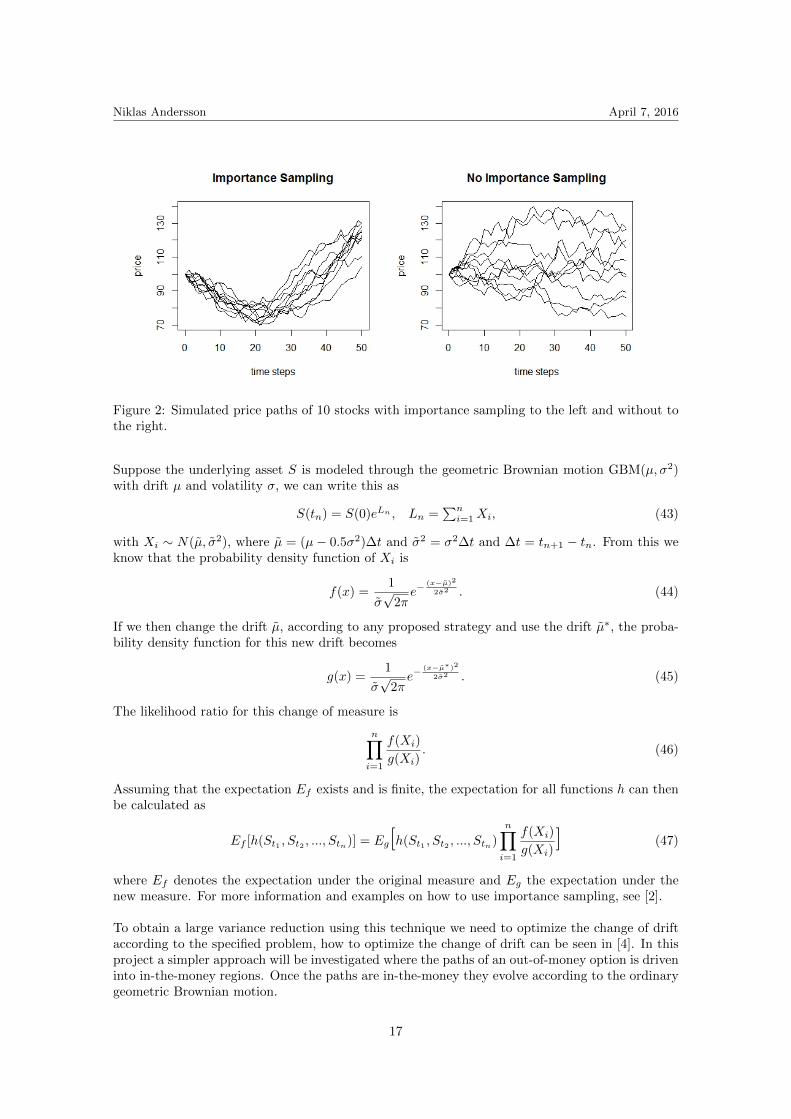
The idea of importance sampling is to change the drift of the underlying assets and drive pathsinto important regions. We would like to drive the paths in such a way that early exercise isenforced and zero-paths vanish, i.e. paths that lie out of money at maturity. To get a feeling ofhow importance sampling can be used and the advantages of the method I have created the plotsin Figure 2 where the paths in the left figure have a change of drift such that they go down to abarrier and up to strike in 50 time steps. This can be compared to the figure where no importancesampling is used. If we for example want to calculate the price of a down-and-in barrier option itwould of course be favorable to use the paths in the left figure.

16


Figure 2: Simulated price paths of 10 stocks with importance sampling to the left and without tothe right.

Suppose the underlying asset S is modeled through the geometric Brownian motion GBM(µ, σ2)with drift µ and volatility σ, we can write this as

S(tn) = S(0)eLn , Ln =∑ni=1Xi, (43)

with Xi ∼ N(µ, σ2), where µ = (µ− 0.5σ2)∆t and σ2 = σ2∆t and ∆t = tn+1 − tn. From this weknow that the probability density function of Xi is

f(x) =1

σ√

2πe−

(x−µ)2

2σ2 . (44)

If we then change the drift µ, according to any proposed strategy and use the drift µ∗, the proba-bility density function for this new drift becomes

g(x) =1

σ√

2πe−

(x−µ∗)2

2σ2 . (45)

The likelihood ratio for this change of measure is

n∏i=1

f(Xi)

g(Xi). (46)

Assuming that the expectation Ef exists and is finite, the expectation for all functions h can thenbe calculated as

Ef [h(St1 , St2 , ..., Stn)] = Eg[h(St1 , St2 , ..., Stn)

n∏i=1

f(Xi)

g(Xi)] (47)

where Ef denotes the expectation under the original measure and Eg the expectation under thenew measure. For more information and examples on how to use importance sampling, see [2].

To obtain a large variance reduction using this technique we need to optimize the change of driftaccording to the specified problem, how to optimize the change of drift can be seen in [4]. In thisproject a simpler approach will be investigated where the paths of an out-of-money option is driveninto in-the-money regions. Once the paths are in-the-money they evolve according to the ordinarygeometric Brownian motion.

17


2.7 Quasi Monte Carlo

Quasi Monte Carlo or low discrepancy methods differ from ordinary Monte Carlo in the waythat they make no attempt to mimic randomness. Let’s consider an example of calculating thediscounted payoff of an European arithmetic put option with d number of assets,

h(s1(T ), ..., sd(T )) = e−rT ·max((K − 1

d

d∑i=1

si(T )), 0). (48)

The price can then be calculated as,

E[h(s1, ..., sn)] =E[e−rT (K −max(1

d

d∑i=1

si(0) · e(r−0.5σ2i )T+σi

√TΦ−1(Ui)), 0)]

= E[f(U1, ..., Ud)] =

∫[0,1)d

f(x)dx.

(49)

Instead of generating pseudo random numbers Ui ∼ U(0, 1) and estimate the integral with 1N

∑Ni=1 f(Ui),

let’s choose X1, X2, ..., XN carefully to fill the hypercube [0, 1)d evenly and use these to estimate

the integral as 1N

∑Ni=1 f(Xi). A sequence that evenly fills the hypercube with dimensions d, [0, 1]d

is called a low discrepancy sequence.

2.7.1 Discrepancy and error estimation

Discrepancy is a measure of how uniformly a sequence is distributed in the unit hypercube. Givena collection A of subsets of [0, 1)d, the discrepancy of the point set x1, ..., xn relative to A is

D(x1, ..., xn;A) = supA∈A

∣∣∣∣#xi ∈ An− vol(A)

∣∣∣∣ , (50)

where #xi ∈ A denotes the number of xi contained in A and vol(A) denotes the volume of A.Taking A to be the collection of all rectangles in [0, 1)d of the form∏d

j=1[uj , vj), 0 ≤ uj < vj ≤ 1, (51)

yields the ordinary discrepancy D(x1, ..., xn). Restricting A to rectangles of the form

d∏j=1

[0, uj) (52)

defines the star discrepancy D∗(x1, ..., xn) [2, p.284]. Suppose that we fix an infinite sequencex1, x2, x3... where every subsequence x1, ..., xn has a low discrepancy. Such a sequence is called a low

discrepancy sequence if the star discrepancy D∗(x1, ..., xn) is of O( log(n)d

n ). The star discrepancyis a central part for error bounds of quasi Monte Carlo integration, and an upper bound for theintegration error is given by the Koksma-Hlawka inequality. The Koksma- Hlawka inequality saysthat if f has a bounded variation V (f) in the sense of Hardy and Krause on [0, 1)d, then for anysequence XN on [0, 1)d the following inequality holds,[2, p.288]∣∣∣∣∣ 1

N

N∑i=1

f(Xi)−∫

[0,1)d]

f(x)dx

∣∣∣∣∣ ≤ V (f)D∗(X1, ..., XN ). (53)

18


This inequality can be compared to the error information available in standard Monte Carlo. Fromthe central limit theorem we know that∣∣∣∣∣ 1

N

N∑i=1

f(Ui)−∫

[0,1)d]

f(u)du

∣∣∣∣∣ ≤ zδ/2 · σf√N , (54)

where Ui ∼ U(0, 1). In comparing the standard Monte Carlo error with quasi Monte Carlo it can beseen that in both cases the error bound is a product of two terms, one dependent on the integrandfunction f and the other on the properties of the sequence. Both V (f) and D∗(X1, ..., XN ) in (53)are extremely hard to compute which leads to the fact that the Koksma-Hlawka inequality haslimited practical use as a error bound. This leads to problems in comparing the quasi Monte Carloestimate with a standard Monte Carlo estimate[12, p.15-16].

2.7.2 Sobol sequence

Sobol sequences are a low discrepancy sequence, and it is probably the most used sequence forhigh dimension integration[12]. For more information of how to create a Sobol sequence and thetheory behind it I refer to P.Glasserman[2] or P.Jackel [5]. In this section I will instead show whySobol sequences are a better choice for high dimensional integration than other low discrepancytechniques. The aim of a low discrepancy sequence is to fill a given domain as evenly and ho-mogeneously as possible, however many techniques lose their capability to produce homogeneoussequences as the dimensions increase [5]. To demonstrate why Sobol’s sequence often is preferredbefore other techniques like Halton’ method I have created Figures 4 and 5 where I have plottedthe projection of the first 1000 points of the Sobol’ sequence and the Halton’ sequence onto atwo dimensional projection of adjacent dimensions. The result of using a pseudo random numbergenerator is illustrated in Figure 3 and you can see that there is no difference in low and high di-mensions. The result of using Sobol’s sequence is seen in Figure 4 and the result of using Halton’ssequence is visible in Figure 5. One can see that the Halton’ sequence does not fill the domainevenly for higher dimensions while Sobol’s sequence still does.

(a) (b) (c)

Figure 3: Pseudo Random numbers

19


(a) (b) (c)

Figure 4: Sobol’s sequence

(a) (b) (c)

Figure 5: Halton’s sequence

2.7.3 Dimensionality Reduction

As mentioned earlier the dimensionality of the problem can be very large when pricing American-style basket options. There are, however, techniques that can be used to lower the effective dimen-sion of the problem. The Principal component analysis can be used to reduce the number of statevariables whereas the Brownian bridge construction can be used to reduce the time dimensions.This is not something that this project focuses on but I will explain the Brownian bridge techniquebriefly and refer to [2] or [12] for further reading.

The Brownian motion, W , is the driving process when simulating stock paths as in (17). It caneasily be generated from left to right by the following recursion

W (ti+1) = W (ti) +√ti+1 − ti zi+1, (55)

where zi+1 is a standard normal random variable and ti+1 > ti. The Brownian bridge constructionprovides an alternative way of generating the Brownian motion where the terminal nodes W (tN )of the paths are determined first. All the intermediate nodes are then added conditional on thealready known realizations of the paths. Suppose that we know two values of the Brownian motionW (ti) and W (tj), we can then use the Brownian bridge construction to calculate an intermediatevalue W (tk) as,

W (tk) =tj − tktj − ti

W (ti) +tk − titj − ti

W (tj) +

√(tk − ti)(tj − tk)

tj − tizk (56)

where ti < tk < tj and zk is a standard normal random variable. Figure 6 illustrates the principleof the method.

20


Figure 6: Illustration of the Brownian bridge construction.

This implies that we can simulate a path of the Brownian motion in any time order. Since manyoptions are more sensitive to the terminal value of the underlying, than of intermediate states, thevariance will be concentrated into large time steps. We can then use the first dimensions of thequasi sequence to control much of the generated paths and use pseudo random numbers for theintermediate steps. Hence getting a lower effective dimensionality[12].

3 Method

This thesis has been performed at Cinnober Financial Technology where I have implementeda system for pricing American-style options on multiple underlying assets using regression basedMonte Carlo. The aim of the first part of the project was to make a comparative study between theLSM method and the RRM method. The LSM method of Longstaff and Schwarz was implementedwith the possibility to replace the solver for regression with robust regression. To compare theresults we focus our attention on the duality approach by Andersen and Broadie. The second partof the project focused on convergence rates therefore the possibility to use Quasi Monte Carlo andimportance sampling were implemented in the system as part of the investigation.

I have also built an n-dimensional extension to the lattice binomial method according to [6] whichhas been used for comparison and verification. This method works very good for the one andtwo asset case but if more assets are used the computational time explodes. For high-dimensionalvaluation problems, the binomial method is not practically useful.

In all the numerical investigations I have assumed that the underlying assets follows a multi-dimensional geometric Brownian motion as in (16). Monte Carlo algorithms are highly dependenton the quality of the random number generator and creating a pseudo-random number is still todaynot a trivial thing. I have used the Mersenne Twister, MT19937, generator to produce uniformpseudo random numbers and the transformation to normal random numbers is made through theBox-Muller method. All code has been written in Java which provides already built in methodsfor generation of both pseudo random numbers and Sobol’s low discrepancy numbers. I could alsouse built in solvers for least square problems. I did not however find any technique to perform

21


robust regression so I had to implement it by myself following the algorithm in [4].

Once working with Monte Carlo and random numbers it is favorable to set a seed in the pseudonumber generator and I have used the linear congruential method to produce a seed vector,

x0 = (as0 + b)modM, xi = (axi−1 + b)modM(57)

where i = 1, ..., 623, s0 = seed = 5, a = 214013, b = 2531011, M = 429496729.

3.1 Algorithms

3.1.1 LSM and RRM

The LSM and RRM algorithm can be summarized as follows

1. Generate N independent paths Snln=1,...,N0,l=1,...,L, according to the multivariate geomet-ric Brownian motion.

2. At the terminal nodes, loop over all paths and set CFn = ZL(SnL), and τn = L.

3. Apply backward induction for l = L− 1 to 1,

• set J = 0, and for n = 1 to N0,

– if(Snl is in-the-money) then

∗ set J = J + 1 and π(J) = n

∗ fill the regressor matrix AJm = φm(Snl), m = 1, ...,M

∗ fill the vector with regressands bJ = e−r(τn−l)∆tCFn

• perform regression to calculate the coefficients βml

• for j = 1 to J do

– C =∑Mm=1 βmlAjm

– if(Z(Sπ(j)l) ≥ C)

∗ set CFπ(j) = Zl(Sπ(j)l) and τπ(J) = l

4. Calculate C0 = 1N

∑Nn=1 e

−rτn∆tCFn

5. Calculate the value of the option by V0 = max(Z0, C0)

Note that the last step of this algorithm implies that the option can be exercised at time 0, i.e.the option can be bought and exercised at the same time step. The number of exercise dates isdetermined in advance in the case of Bermudan options and in my numerical investigations I didnot allow exercising at time 0, instead the option was evaluated as V0 = C0. As can be seen in thealgorithm above we can easily switch between robust regression and least square regression oncethe algorithm has been implemented. Just change the regression part where the coefficients βmlare calculated.

If we like to use another set of S2nln=1,...,N2,l=1,...,L to evaluate the option and hence separate the

determination of coefficient part and the evaluation part we can easily do so. Follow the steps 1-3in the algorithm above to determine the regression coefficients in each time step but replace step4 and 5 with

22


4. Generate a new set of independent paths S2nln=1,...,N1,l=1,...,L, according to the multivariate

geometric Brownian motion.

5. for n = 1 to N1 do

• set l = 1 and C =∑Mm=1 βmlφ(S2

nl)

• while (Z(S2nl) ≤ 0 or Z(S2

nl) < C and l 6= L) do

– update l=l+1 and C =∑Mm=1 βmlφ(S2

nl)

• set CF ∗n = Z(S2nl) and τ∗n = l

6. Calculate C0 = 1N

∑Nn=1 e

−rτ∗n∆tCF ∗n

7. Calculate the value of the option by V0 = max(Z0, C0)

3.1.2 Duality approach

In the following subsection I will go through the Andersen and Broadie algorithm that I use tocreate a lower and upper estimate of the option price.

1. Run the LSM / RRM method with a set of S0nln=1,...N0,l=1,...,L paths and determine the

coefficients that define the stopping criterion τ at each time step such as given by τl =infk ≥ l|Zl ≥ Cl.

2. Estimate the lower bound L0 by simulating a new set of paths S1nln=1,...,N1,l=1,...,L and

stopping according to the τ1

L0 =1

N1

N1∑n=1

e−rτn1 ∆tZnτn1 . (58)

A valid (1− α) confidence interval of L0 can be created by

L0 ± z1−α/2

√σ2L

N1(59)

with σL being the estimated standard deviation of L0 and z1−α/2 denotes the (1 − α/2)quantile of a standard normal distribution.

3. The upper bound U0 is given as,

U0 = E0[ maxl=1,...,L

(e−rl∆tZl −Ml)]+M0 =: ∆0 +M0 (60)

with M0 = E0[e−rτ1∆tZτ1 ], Ml = Ml−1 + El[e−rτl∆tZτl ] − El−1[e−rτl∆tZτl ] =: Ml−1 + δl,

l = 1, ..., L, and

El[e−rτ1∆tZτl ] =

e−rl∆tZl, if Zl ≥ ClEl[e

−rτl+1∆tZτl+1], if Zl < Cl

. (61)

To estimate the upper bound U0 we simulate another set of N2 paths S2nln=1,...,N2,l=0,...,L

to approximate ∆0 in (60) by

∆0 :=1

N2

N2∑n=1

∆n (62)

23


where∆n = max

l=1,...,L(e−rl∆tZnl −Mn

l ),Mnl = Mn

l−1 + δnl

and evaluate δnl by

δnl =

e−rl∆tZnl , if Znl ≥ Cl(S2

nl)

Cnl , if Znl < Cl(S2nl)

− Cnl−1

where Cnl are the result of running a simulation in the simulation, i.e. creating N3 new pathsS3nkn=1,...,N3,k=l,...,L stating at S2

nl and stopping according to τl+1,

Cnl =1

N3

N3∑m=1

e−rτml+1∆tZmτml+1

. (63)

4. From the results of the procedure above an upper bound U0 can be created

U0 = ∆0 + L0

and a valid 100(1− α)% confidence interval for U0 is given by

U0 ± z1−α/2

√σ2L

N1+σ2

∆

N2(64)

where σ∆ is the estimated standard deviation of ∆0.

5. A valid 100(1−α)% confidence interval for the true option value can then be determined by[L0 − z1−α/2

σL√N1

, U0 + z1−α/2

√σ2L

N1+σ2

∆

N2

]. (65)

4 Results

In this section I will present some numerical results. To start with I concentrate on investigatingdifferences between the robust regression and the least square regression techniques, this is subsec-tion 4.1. The subsections 4.2 and 4.3 are about speeding up the convergence rates via Quasi MonteCarlo and importance sampling. In subsection 4.4 I combine the methods Quasi Monte Carlo andimportance sampling with the RRM method and compare it to the LSM method.

4.1 LSM vs RRM

To investigate how the choice of basis functions influence the result I created Table 4 where theprice of a max call option on 2 assets has been calculated using both least square regression(LSR) and robust regression (RR) with different basis. The payoff of this option is Z(s1, s2) =max(0,max(s1, s2)−K) and the value of these calculations can be compared with the result fromthe binomial tree, 8.0735. From the results in Table 4 it is clear that the choice of basis affects theresults and if one compares with the value from the binomial tree it seems as if it is preferable tochoose a basis that includes the payoff, Z(s1, s2) and interaction terms s1s2.

24


Table 4: Option value of Bermudan max call option on 2 stocks for LSR, RRHuber and RRJonenmethod with different basis.

Basis LSR RRHuber RRJonen

s3i , s

2i , si, 1 8.00 7.96 7.95

s1s2, s3i , s

2i , si, 1 8.02 8.02 8.01

max(s1, s2), s1, s2, s3i , s

2i , si, 1 8.05 8.06 8.08

s1s22, s

21s2, s1s2, s

3i , s

2i , si, 1 8.04 8.02 8.02

Z(s1, s2), s1s22, s

21s2, s1s2, s

3i , s

2i , si, 1 8.03 8.05 8.05

Z(s1, s2), s1s2, s2i , si, 1 8.05 8.06 8.06

Notes. Common option parameters are T=3, exercise opportunities = 9,K=100, Si

0 = 90,i = 1, 2. r=0.05, δd = 0.1 d = 1, 2, σd = 0.2 d = 1, 2,ρ1,2 = 0. Results are created using the average of 10 runs and 100000replications in each run with α = 0.92, β = 0.993. The result from thebinomial tree is calculated with 360 time steps an is 8.0735.

The values in Table 4 have been calculated with the parameters α = 0.92 and β = 0.993 fordetermining transition points. Now, using the base Z(s1, s2), s1s2, s

2i , si, 1 from Table 4 I instead

examine the effect of different transition points on the same option. The results can be seen inFigure 7, the first three points from the left are the prices using Huber’s loss function with differentvalues of α, the following 9 points are the prices using Jonen’s loss function with different α and β.The two points to the right are the prices calculated using least square regression (LSR). The linecorresponds to the value of the binomial tree from 360 time steps. The transition points clearlyaffect the results and remembering that these estimations actually are low estimates of the optionprice it is a good sign that the values from robust regression are higher than the least squareregression values.

Figure 7: Price of max call option on 2 assets with different transition points in the robust regressionmethod. S0 = 90 for both stocks. Basis according to Entry 6 in Table 4. The results are based onthe average of 10 runs and 100000 replications per run. For other option parameters see the notesin Table 4.

If we for a moment try and forget about the Andersen and Broadie’s approach and try to investigatedifferences between the RRM and LSM methods without the duality approach we will see thatit is quite hard to find any differences. In Table 5 I have priced a max call option on 2,3 and 5

25


underlying assets using both RRM with Huber’s loss function and LSM. These values can then becompared to the value from the binomial tree (in 2 and 3 asset case). It seems that we get slightlysmaller confidence intervals and a little higher estimates using robust regression. I use differentbasis depending on the number of assets and these are according to

Z(s1, s2), s1s2, s21, s

22, s1, s2, 1, (66)

1, s1, s2, s3, s21, s

22, s

23, s

31, s

32, s1s2, s1s3, s2s3, s

21s2, s1s

22, (67)

1, s1, s2, s3, s4, s5, s21, s

22, s

23, s

24, s

25, s

31, s

32, s1s2, s1s3, s2s3, s

21s2, s1s

22, (68)

for the 2, 3 resp 5 asset case where the stock prices has been ordered such that s1 > s2 > · · · > sd.

Table 5: Calculated 95% confidence interval using LSM and RRM method for Bermudan max calloption on 2, 3 and 5 assets.

Nr of assets S0 Method 95% CI Size CI Est. Price Binomial tree

2

90LSM [7.9658, 8.1130] 0.154 8.0420

8.0735RRM [7.9828, 8.1334] 0.151 8.0581

100LSM [13.745, 13.937] 0.192 13.841

13.901RRM [13.781, 13.970] 0.189 13.875

110LSM [21.181, 21.404] 0.223 21.292

21.354RRM [21.205, 21.427] 0.222 21.316

3

90LSM [11.167, 11.341] 0.174 11.254

11.322RRM [11.177, 11.348] 0.171 11.262

100LSM [18.566, 18.782] 0.216 18.674

18.692RRM [18.575, 18.789] 0.213 18.682

110LSM [27.443, 27.691] 0.249 27.567

27.620RRM [27.426, 27.675] 0.249 27.551

5

90LSM [16.531, 16.734] 0.203 16.632

-RRM [16.522, 16.723] 0.201 16.623

100LSM [26.025, 26.267] 0.242 26.146

-RRM [26.037, 26.278] 0.241 26.158

110LSM [36.574, 36.847] 0.273 36.711

-RRM [36.617, 36.891] 0.274 36.754

Notes. Common option parameters are T=3, exercise opportunities = 9, K=100, r=0.05,δd = 0.1 d = 1, ...5, σd = 0.2 d = 1, ..., 5, ρde = 0 ∀d 6= e. For the Binomial tree 360 time stepsare used for 2 asset, and 90 time steps for 3 assets. The number of paths in MC calculationsare 100000 and repeated 10 times. Basis for 2 assets are according to (66), for 3 assets (67),and for 5 assets (68). The transition points α = 0.90 with Huber loss function.

To compare the variances between the methods I have also plotted the standard error for the 2assets case and S0 = 100 for both stocks, see Figure 8. From the results in Table 5 and Figure 8it is hard to say that one method is better than the other.

26


Figure 8: Standard error calculated with robust regression and least square regression for Bermudanmax call option on 2 stocks. S0 = 100 for all stocks, see Table 5 for other option parameters.

To try and find differences between the RRM and LSM technique before adding the technique ofAndersen and Broadie I created the histograms in Figure 9 and the density plot in Figure 10. Inthese figures I have calculated the price of a max call option on 3 and 5 assets 2500 resp 1500 timesusing 100000 paths per run. In the density plot I have also added the value calculated with thebinomial tree for the 3 asset case (18.69). From the density plot one can see that the distributionsdiffer a little bit and again we see that the values calculated with the RRM technique are higherthan the LSM. From these figures it seems as if the data are normally distributed and this cannot be rejected with statistical tests. Therefore I also do a two-sided student t-test to test if themean from the two populations are equal, and this test shows that there is a significant differencebetween the mean of the 2 distributions. However if I also do a test to check for equal variances thistest does not fail and hence strengthen the belief that the variances between the populations doesnot differ. An interesting note from the histograms is that there appears to be more ”extreme”values from the LSM method, i.e. values that lies below 18.55 in 3 asset case and below 25.95 inthe 5 asset case.

27


(a)

(b)

Figure 9: Histogram of the price of a max call option on 3 and 5 assets. See table 5 for parametersettings.

28


(a)

(b)

Figure 10: Density plot of the price of a max call option on 3 and 5 assets. See table 5 for parametersettings.

4.1.1 Duality approach

If we add the method of Andersen and Broadie and thus create both an upper and lower boundfor the option price we will see that it is easier to find differences between the RRM and LSMmethods. In Table 6 I have priced an arithmetic call option on 5 assets, the payoff for this optionis given by

Z(s1, s2, s3, s4, s5) = max(0,(s1 + s2 + s3 + s4 + s5)

5−K).

The basis that I use is according to

1, s1, s2, s3, s4, s5, s21, s

22, s

23, s

24, s

25, (69)

29


and to make a fair comparison of the methods I set a seed in the pseudo number generator accordingto (57). In the table I calculate both a lower and upper bound of the option price (standard errorin the parenthesis) and a 95% confidence interval according to (65). The ∆ ratio is simply thedifference between the high and low estimator from the LSM approach divided with the differencebetween the high and low estimator from the RRM approach. The tighter between the lower andupper bound and the higher the lower bound the more accurate is the approximated early exercisestrategy, therefore this ∆ ratio can be used to compare the methods. As can be seen in Table 6we get higher lower bounds and tighter upper bounds with the RRM method using both Huber’sloss function and Jonen’s loss function compared to the LSM method. The confidence intervalsare smaller and we can see a slight reduction in variance using robust regression. The ∆ ratios arebetween 2.5 and 4.

Table 6: Low estimator, High estimator and a calculated 95% confidence interval for a Bermudanarithmetic average call option on 5 asset, using both LSM and RRM method.

S0 Method Low High 95% CI Size CI ∆ Ratio

90LSM 1.534 (0.0048) 1.554 (0.0057) [1.525, 1.565] 0.040

RRM, Huber 1.545 (0.0046) 1.552 (0.0048) [1.536, 1.561] 0.025 3.1RRM, Jonen 1.546 (0.0045) 1.552 (0.0047) [1.537, 1.561] 0.024 3.2

100LSM 3.955 (0.0068) 3.995 (0.0077) [3.942, 4.010] 0.068


110LSM 9.313 (0.0078) 9.371 (0.0091) [9.298, 9.389] 0.091


Notes. Common option parameters are T=3, exercise opportunities = 9, K=100, r=0.05, δd = 0.1d = 1, ...5, σd = 0.08 + 0.08 · d d = 1, ..., 5, ρde = 0 ∀d 6= e. The number of paths in MC calculationsare N0 = 400000, N1 = 1000000, N2 = 1500, N3 = 8000. Basis are according to (69). The transitionpoints are α = 0.9 for Huber and α = 0.87 and β = 0.993 with Jonen’s loss function.

In Table 7 I again use the seed in (57) but change the option to a max call option on 2 assets anduse the base according to (66). I calculate low and high estimates, 95% confidence intervals and ∆ratios. For this option benchmarks values can be calculated using the binomial tree, and these are8.074, 13.90 and 21.35. It can be seen that the calculated confidence intervals cover these ”true”values and again we see that we get higher lower bounds and tighter upper bounds using the RRMmethod compared to the LSM method. The ∆ ratios are not as large as in Table 6 but they arebetween 1.4 and 2.4.

30


Table 7: Low estimator, High estimator and a calculated 95% confidence interval for a Bermudanmax call option on 2 asset, using both LSM and RRM method.


90LSM 8.044 (0.012) 8.075 (0.013) [8.020, 8.100] 0.080


100LSM 13.866 (0.0155) 13.918 (0.0163) [13.836, 13.950] 0.115

RRM, Huber 13.888 (0.0153) 13.917 (0.0157) [13.858, 13.948] 0.0903 1.7RRM, Jonen 13.895 (0.0152) 13.921 (0.0155) [13.865, 13.952] 0.0861 2

110LSM 21.289 (0.0180) 21.378 (0.0192) [21.253, 21.415] 0.162


Notes. Common option parameters are T=3, exercise opportunities = 9, K=100, r=0.05, δd = 0.1d = 1, 2, σd = 0.2 d = 1, 2, ρde = 0 ∀d 6= e. The number of paths in MC calculations are N0 = 400000,N1 = 1000000, N2 = 1500, N3 = 8000. Basis are according to (66). The transition points are α = 0.9for Huber and α = 0.87 and β = 0.993 with Jonen’s loss function.

The values in Table 8 have been created without any seed set in the pseudo number generator. Inthis table I have priced a max call option on 5 underlying assets using the base in (68). We see aslight reduction in variance and ∆ ratios between 1.2 and 1.6 in this case.

Table 8: Low estimator, High estimator and a calculated 95% confidence interval for a Bermudanmax call option on 5 asset, using both LSM and RRM method.


90LSM 27.398 (0.0329) 27.685 (0.0377) [27.334, 27.758] 0.425


100LSM 37.614 (0.0380) 38.131 (0.0479) [37.539, 38.225] 0.686


110LSM 49.116 (0.0416) 49.627 (0.0491) [49.034, 49.723] 0.689


Notes. Common option parameters are T=3, exercise opportunities = 9, K=100, r=0.05, δd = 0.1d = 1, ..., 5, σd = 0.08 + 0.08 · d d = 1, ..., 5, ρde = 0 ∀d 6= e. The number of paths in MC calculations areN0 = 400000, N1 = 1000000, N2 = 1500, N3 = 8000. Basis are according to (68). The transition pointsare α = 0.9 for Huber and α = 0.87 and β = 0.993 with Jonen’s loss function.

4.2 Quasi MC

To examine the effect of Quasi Monte Carlo I price a max call option on 2 asset with the same optionparameters as in table 5 and valuate the option with the same paths that I use to determine theexercise strategy. As can be seen in Figure 11 the values calculated with Sobol numbers convergemuch faster and stays stable compared to when pseudo random numbers are used. It looks as if

31


the values calculated using Sobol numbers are stable already after 50000 paths. The value fromthe Binomial tree has also been plotted for comparison.

Figure 11: Bermudan max call option on 2 stocks, S0 = 100 for both stocks valuated using robustregression with both pseudo random numbers and Sobol numbers. The value calculated with thebinomial tree is 13.90 for comparison. see Table 5 for other parameters.

The same striking result can be seen in Figure 12 and 13 where the lower bound for a max calloption on 2 resp 3 assets has been determined using both Sobol numbers and pseudo randomnumbers but the same exercise strategy.

32


Figure 12: Convergence of Low estimator using least square regression with pseudo random num-bers and Sobol numbers. For Bermudan max call option on 2 stocks. S0 = 90 for both stocks, seeTable 7 for other option parameters. N0 = 500000.

Figure 13: Convergence of Low estimator using least square regression with both pseudo randomnumbers and Sobol numbers. For Bermudan max call option on 3 stocks. S0 = 100 for both stocks,see Table 7 for other option parameters. N0 = 500000.

33


4.3 Importance Sampling

In Table 9 I have calculated the lower bound of an arithmetic average call option on 3 assets withexpiry date of both 1 and 3 years using both importance sampling and no importance sampling.The option is an out-of-money (OTM) option with S0 set to 90 and strike price K set to 100. In thecase of importance sampling I set the drift of the assets so that the option is in-the-money (ITM)after 4 time steps, thereafter the paths will evolve according to the ordinary geometric Brownianmotion. To calculate the results I use the base

1, s1, s2, s3, s21, s

22, s

23, (s1 + s2 + s3)/3, (70)

and use LSM method to determine the exercise strategy. The seed is set according to (57). Theresults show that we can calculate the lower bound with a much smaller standard error (SE) usingimportance sampling than when no importance sampling is used. The results also indicate thatthe importance sampling technique gives a more striking result the more unlikely the outcome is.

Table 9: Low estimator and standard error for an arithmetic average call option on 3 assets withmaturity date 1 and 3 years.

Method T=1 T=3Low estimator SE Low estimator SE

Standard MC 0.47377 0.0019 1.0964 0.0034Import. Samp 0.47302 0.00061 1.0961 0.0013Binomial tree 0.47622 1.0910

Notes. Common option parameters are, exercise opportunities = 9, K=100,S0 = 90 for all assets, r=0.05, δd = 0.1 d = 1, 2, 3, σd = 0.2 d = 1, 2, 3,ρde = 0 ∀d 6= e. For the Binomial tree 90 time steps are used. The numberof paths in MC calculations are N0 = 500000 and N1 = 1000000. Seed isset according to (57) and basis according to (70). Early exercise regions arecalculated with the LSM. The drift when using importance sampling is setso that at-the-money is reached after 4 time steps.

I also create a convergence plot of the low estimator for the same option and using the sameparameters as in the example above but without any seed set (the exercise strategy is the samein both cases). One can see that the low estimator seems to be too high compared to the truevalue created by the binomial tree. A more interesting result can be seen in Figure 15 where thestandard error has been plotted. There is clearly a big difference between the case when importancesampling is used compared to when it is not.

34


Figure 14: Convergence of Low estimator using least square regression with and without importancesampling. For Bermudan arithmetic average option on 3 stocks. S0 = 90 for both stocks and T = 3.See Table 9 for other option parameters. N0 = 500000, no seed set but uses the same coefficientsin both cases.

Figure 15: Standard error of Low estimator using least square regression with and without impor-tance sampling. For Bermudan arithmetic average option on 3 stocks. S0 = 90 for both stocksand T = 3. See Table 9 for other option parameters. N0 = 500000, no seed set but uses the samecoefficients in both cases.

35


4.4 Combinations

As a final result I create a convergence plot of both the low- and high estimation of the price ofan arithmetic average call option on 2 assets using the base

1, s1, s2, s21, s

22, s

31, s

32. (71)

I do this using both the least square technique and the robust regression technique to determinethe exercise strategy. Once the exercise strategy has been determined I calculate the lower andupper bound using the exercise strategy determined by least squares without any quasi numbersor importance sampling. I also calculate lower and upper bound using the exercise strategy fromrobust regression but then I add quasi numbers and importance sampling. Importance sampling isonly used to calculate the lower bound and the drift is set so that in-the-money regions is reachedafter 4 time steps. The results can be seen in Figure 16 and it is clear that the results using robustregression give a much smaller interval than the least square regression, this can also be seen inFigure 17 where I plot the difference between the upper and lower bound for both cases. It is alsoclear that the the values calculated using Sobol numbers and importance sampling converges muchfaster than when pseudo random numbers are used.

Figure 16: Upper and lower bounds calculated for an arithmetic average call option on 2 assetsusing both LSM with pseudo random numbers and RRM combined with Sobol numbers andimportance sampling to calculate the lower bound and Sobol numbers to calculate upper bound.The calculations with robust regression are made with Jonens loss function using α = 0.87 andβ = 0.993. S0 = 90 for both stocks and T = 3. See Table 9 for other option parameters.N0 = 300000, N1 varies between 10000 and 500000, N2 between 100 and 500, N3 between 200 and1500. Seed is set when calculating coefficients.

36


Figure 17: Difference between upper and lower bound from Figure 16.

5 Discussion

This project has considered the pricing procedure of multi-dimensional American-style options.Regression-based Monte Carlo techniques has been used to determine early exercise strategies andtwo different regression procedures to calculate continuation values has been evaluated. It appearedto be hard to find advantages or differences between the methods without the duality approach ofAndersen and Broadie therefore this method was added. Using this method it was shown that therobust regression technique provide a higher lower bound and a tighter upper bound. The resultsshow that we can get as much as 4 times smaller intervals using the robust regression technique.

A recurrent question when using regression-based Monte Carlo is how to choose the basis functions.This is a topic of its own and there are a lot of articles on this subject. However this is notsomething that this project has focused on more than to verify that the choice has a big impacton the result and therefore definitely something that should be taken into consideration in furtherwork. Another problem that appears when using robust regression is how to choose loss functionand transition points, in this project I have only considered Huber’s loss function and the lossfunction recommended by C.Jonen [4], but other loss functions should also be tested in futurework. Regarding the transition points I mainly focused on the result from Figure 7 and usedvalues of 0.87 or 0.90 for α and 0.993 for β, these values also coincide with the ones that C.Jonenuses in most of his numerical investigations.

Another factor that might impact the result from the regression step is whether or not to use ”only-in-the-money” paths once performing the regression. There are different opinions regarding thisquestion, Longstaff and Schwarts [3] and C.Jonen [4] recommend using only in-the-money pathswhile P.Glasserman [2], recommends to use all paths. This is a question that should be investigatedfurther since I found that the results might differ quite a lot depending on the choice. In Table 11in the Appendix 6.2 I have replicated Table 9 from section 4.3 but using all paths in the regression

37


step and it can be seen that the result differs a lot. It might be that OTM options that are notvery volatile are more sensitive to the choice of using only in-the-money-paths or not. The reasonof using only in-the-money-paths in the regression is that the zero values will affect the regressionso that we get inferior results, but it is also less time consuming to use only in-the-money-paths.In the case of an OTM option that is not very volatile there will be very few paths that are in themoney and hence the regression will be based on a very small set of paths, therefore the resultsof using only in the money paths will differ more than if there are a lot of paths that are in themoney. This is something that should be investigated further in order to make some conclusionsregarding when to use only in-the-money-paths and when to use all paths.

In this project we have focused on Bermudan options. i.e. options that only can be exercisedat a final set of exercise opportunities. The step to pricing American options is not very largesince we can always just increase the number of exercise opportunities. However, if the exerciseopportunities increase the number of evaluation steps also increases and for multi-dimensionaloptions the memory demand gets very large. Therefore it might be recommended to work withdimensionality reduction techniques. For many options it is enough to only create values for onetime step at a time, therefore the Brownian bridge technique should be implemented to reduce theamount of memory needed once evaluating these options.

The second part of this project focused on variance reduction and therefore the use of low dis-crepancy sequences was considered instead of pseudo random numbers. Due to the superiority inhigher dimensions Sobol’s technique was chosen and investigated. It is problematic to calculateerror estimates for Sobol’ sequences therefore it is hard to compare the method to pseudo randomnumbers but it can be seen in the convergence plots that the results using Sobol numbers convergemuch faster than when pseudo numbers are used. A drawback of low discrepancy techniques is thatthey lose their strength for higher dimensions, I have however not noticed this in my numericaltests and due to the striking improvement of convergence rate I really recommend this technique.Already implemented methods for creating Sobol numbers are usually available in most program-ming languages therefore it is also very easy to implement this technique into an already runningoption pricing system.

Importance sampling has also been considered in this project, this technique is not as easilyimplemented as Quasi Monte Carlo but requires a lot from the user. The method has the potentialto reduce the variance significantly and can be especially useful when pricing path dependentoptions, like the barrier option. I spent a lot of time trying to make the importance sampling worktogether with the regression part until I finally realized that these methods are highly incompatiblewith each other. Using importance sampling before the regression often led to American optionsbeing valuated as European options because the calculated exercise strategies never suggestedexercise in advance. Therefore, in this project, I only considered a change of drift such that thepaths of an OTM option were driven into in-the-money regions and then I let the paths evolveaccording to the ordinary geometric Brownian motion. Using this strategy, importance samplingcould be used together with the regression because the option will never be exercised until beingin-the-money. If the paths reached in-the-money regions after about half of the total number oftime steps the variance reduction was as largest. Later I realized that you can separate betweendetermining the exercise strategy and valuating the option. In this case, importance sampling canbe used in the valuation part but not for determining the exercise strategy. I did not have enoughtime to work further with the importance sampling but I think that if more efforts should be puton this subject it would be preferable to consider algorithms for solving the underlying stochasticoptimization problem like C.Jonen[4] does with a great success.

I have not made any comparison of the computational time between the methods in this project,this is because a fair comparison is hard to accomplish. When robust regression is used the residualsneed to be ordered (I have used Quicksort, O(nlogn)), so it is natural that the computational time

38


is larger with this method which I also have noticed in the numerical investigations. But sincethe results are more accurate using robust regression it is not a fair comparison. To make a faircomparison one could instead try and run the LSM with more basis functions than the RRM andcompare the time for a certain level of ∆ ratio to be reached. Like I mentioned in the methodsection I implemented the robust regression method myself while I use an already built in methodfor least square regression. Therefore if an investigation of CPU time was considered one wouldhave to use the robust regression implementation but with the loss function of ordinary least square(OLS) so that the implementation does not affect the result. To make a comparison between theCPU time of the implemented variance reduction techniques one could run the algorithms until acertain level of the standard error is reached and compare the results.

Another interesting topic for future work is the change of the underlying model. In this projectI have assumed that the assets can be modeled through the geometric Brownian motion, where Ihave assumed a constant interest rate and volatility. It would be interesting to instead investigatethe use of non constant volatility models, i.e. models where the volatility is a function of price andtime. Examples of such models are the Heston model explained in [8] and the model explained byTullie [7].

6 Appendix A1

6.1 Importance sampling example

Let’s say we want to estimate θ = P (X > 4) when X is a standard random variable X ∼N (0, 1). The naive way to estimate θ is by generating X1, X2, ... XN from N (0, 1) and using

θ = 1N

∑Ni=1 1Xi>4 as an estimate where 1Xi>4 is equal to 1 if Xi > 4 and zero otherwise. The

problem using this naive approach is that it is very unlikely to get a Xi > 4 and we will have to usea large number of random numbers to get an estimate that is not zero. If we instead use importance

sampling we change the distribution that Xi are sampled from and use θIS = 1N

N∑i=1

1Xi>4f(Xi)g(Xi)

as

our estimator where Xi are sampled under g(x). Let’s use exponential tilting to find the probabilitydensity g(x) of this new distribution,

g(x) =etxf(x)

M(t).

where M(t) is the Moment generating function,

M(t) = Ef [etx] =

∫Retxf(x)dx =

∫Retx

1√2πe−x

2/2dx =

∫R

1√2πetx−x

2/2dx =∫R

1√2πe

−(x2−2tx−t2+t2)2 dx = et

2/2

∫R

1√2πe−(x−t)2/2dx = et

2/2,

(72)

where I have used∫

R1√2πe−(x−t)2/2dx = 1. We can now construct g(x),

g(x) =etxf(x)

M(t)=etx 1√

2πe−x

2/2

et2/2=

1√2πe

−(x−t)22 . (73)

Hence we should sample X1, X2, ... XN from N (t, 1). The next step is to determine the optimal t.In the general case when we are trying to calculate P (x > a) the optimal t is such that Eg(Xi) = a,

39


where the subscript g meaning that Xi are sampled from the exponential tilted density g(x). Sincewe know that Eg[Xi] = t we can directly see that the optimal t is t = 4 for this particular problem.

We can now construct the importance sampling estimator as,

θIS =1

N

N∑i=1

1Xi>4f(Xi)

g(Xi)

where Xi are sampled from the density function g(x). In Table 10 are the results from using boththe naive approach and importance sampling approach to estimate P (Xi > 4), where Xi ∼ N (0, 1).These results can be compared to the real value of P (Xi > 4) = 3.1671 · 10−5.

Table 10: The estimated value of θ = P (Xi > 4) using both naive Monte Carlo and importancesampling for N = 1000, 10000, 100000, 1000000 simulations.

Method N=1000 N=10000 N=100000 N=1000000

Naive 0 0 1.0000 · 10−5 2.9000 · 10−5

Importance sampling 2.9738 · 10−5 3.2881 · 10−5 3.1897 · 10−5 3.1655 · 10−5

6.2 Not only in-the-money paths

Table 11: (Not only in the money path) Low estimator and standard error for an arithmetic averagecall option on 3 assets with maturity date 1 and 3 years.

Method T=1 T=3Low estimator SE Low estimator SE

Standard MC 0.44693 0.0015 1.0746 0.003Import. Samp 0.44762 0.00047 1.0719 0.0011Binomial tree 0.47622 1.0910

Notes. Common option parameters are, exercise opportunities = 9, K=100,S0 = 90 for all assets, r=0.05, δd = 0.1 d = 1, 2, 3, σd = 0.2 d = 1, 2, 3,ρde = 0 ∀d 6= e. For the Binomial tree 90 time steps are used. The numberof paths in MC calculations are N0 = 500000 and N1 = 1000000. Seed isset according to (57). Basis are according to (70). Early exercise regions arecalculated with the LSM. The drift when using importance sampling is setso that at-the-money is reached after 4 time steps.(Not only in-the-moneypaths are used in the regression step)

References

[1] John C. Hull, OPTIONS, FUTURES, AND OTHER DERIVATIVES, Pearson Education,8th edition, 2012.

[2] Paul Glasserman, Monte Carlo Methods in Financial Engineering, Springer Science, 2003.

40


[3] Francis A. Longstaff, Eduardo S. Schwartz, Valuating American Options by Simulation: ASimple Least-Squares Approach, The Review of Financial Studies, Vol 14 No.1,pp. 113-147,2001.

[4] Christian Jonen, Efficient Pricing of High-Dimensional American-Style Derivatives: A RobustRegression Monte Carlo Method, PhD dissertation University Koln, 2011.

[5] Peter Jackel, Monte Carlo Methods in Finance, John Wiley & Sons, 2002.

[6] P. Boyle, J. Evinine, S. Gibbs, Numerical Evaluation of Multivariate Contingent Claims, Thereview of Financial Studies Vol 2 number 2 pp. 241-250, 1989.

[7] Tracey Andrew Tullie, Variance Reduction for Monte Carlo Simulation of European, Americanor Barrier Options in a Stochastic Volatility Environment., North Carolina State University,2002.

[8] Steven L. Heston, A closed- Form Solution for Options with Stochastic Volatility with Ap-plications to Bond and Currency Options, The review of Financial Studies Vol. 6 No. 2 pp.327-343, 1993.

[9] Leif Andersen, Mark Broadie, Primal-Dual Simulation Algorithm for Pricing Multidimen-sional American Options, Management Science Vol. 50 No.9 pp. 1222-1234, 2004.

[10] Mark Broadie, Paul Glasserman, Pricing American-style securities using simulation, Journalof Economic Dynamics and Control vol. 21 pp. 1323-1352, 1997.

[11] Espen Gardeer Haug, The Complete Guide To Option Pricing Formulas, McGraw-Hill Pro-fessional, Second Edition, 2007.

[12] d-fine GmbH, Valuation of American Basket Options using Quasi-Monte Carlo Methods, MScin Mathematical Finance Trinity Term 2009, University of Oxford

[13] Tomas Bjork, Arbitrage Theory in Continuous Time, Oxford University Press, third edition,2009

[14] L.C.G Rogers, Monte Carlo valuation of American options, Mathematical Finance 12:271-2862002

41

Regression-Based Monte Carlo For Pricing High-Dimensional ...

Documents

Transcript of Regression-Based Monte Carlo For Pricing High-Dimensional ...