Price Comovement and Time Horizon: Fads and...
42
Price Comovement and Time Horizon: Fads and Fundamentals Working Paper Robert Turley * July 2012 * Harvard University Department of Economics and Harvard Business School. Baker Library 220D, Boston MA 02163. Email [email protected]. I am grateful for helpful comments from Robin Greenwood, John Campbell, Josh Coval, Jeremy Stein, Malcolm Baker and various seminar participants.
Transcript of Price Comovement and Time Horizon: Fads and...

Price Comovement and Time Horizon:
Fads and Fundamentals
Working Paper
Robert Turley∗
July 2012
∗Harvard University Department of Economics and Harvard Business School. Baker Library 220D, Boston MA02163. Email [email protected]. I am grateful for helpful comments from Robin Greenwood, John Campbell,Josh Coval, Jeremy Stein, Malcolm Baker and various seminar participants.

Abstract
Investors weigh the shared risk exposures of financial assets through the comovement of their prices.However, to the extent that short-run price variation is transient, the correlation of short-horizonreturns may be inconsistent with the correlation of long-horizon returns. An empirical analysisof US equity prices shows strong evidence for this sort of inconsistent price comovement. Thedifference between long-horizon and short-horizon correlations for two securities can be predictedby contrasting measures of their trading behavior with their shared fundamental exposures. Thishas implications for portfolio construction for long-term, buy-and-hold investors and for investorswho wish to tactically profit from predictability in correlations.
JEL classification: G02, G11, G14

1 Introduction
A portfolio’s investment risk is closely connected to the comovement of its components; risk
diversifies when price movements are independent but persists when changes in price are correlated.
But what if prices move together over short time intervals but seem less related over long horizons?
It would seem they share exposure to a fad that is unrelated to fundamental risk or profitability. In
other cases, closely related assets might have prices that move together over long horizons but not
over shorter intervals. This insufficient comovement masks their shared fundamental exposures.
Analyzing the returns to individual US equities, I find their correlations depend significantly on
the time horizon considered. For each pair of stocks, measures of shared trading behavior versus
measures of shared fundamentals are highly predictive of excess or insufficient comovement.
My empirical results employ a novel methodology in estimating how much of the measured
differences in short-horizon and long-horizon correlations arise from estimation noise. This drives
the statistical inference, emphasizing that these differences are too large to be circumstantial. The
weekly returns to a typical pair of US stocks have a correlation of 18%, but I find the correlation of
their 6-month returns are frequently 20% higher or lower than their weekly returns would suggest.
Long-horizon correlations predictably decrease for stocks with similar investor trading patterns
and correlations predictably increase for stocks of firms with closely related business prospects as
measured by their industry affiliation or by past accounting measures.
In contrast with previous studies studying excess comovement by looking for special cases where
nominal labels change but fundamental risks do not, I take the broad universe of US stocks and
analyze comovement through differences in short-run and long-run correlations. The methodology
could easily be employed within or across other asset classes.
Correlations are a key ingredient in asset allocation and asset pricing, and these findings have
practical implications for investors. Estimates of portfolio risk should depend on the time horizon.
Buy-and-hold investors may be misled if their diversification estimates are based on short-term
returns. Short-horizon correlations will be much more pertinent to an investor who rebalances
frequently. Such an investor might also take advantage of the associated predictability. A simple
long/short trading strategy based on a measure of fads versus fundamentals generates risk-adjusted
annual excess returns of 8.4% and a Sharpe Ratio of 1.03.
1
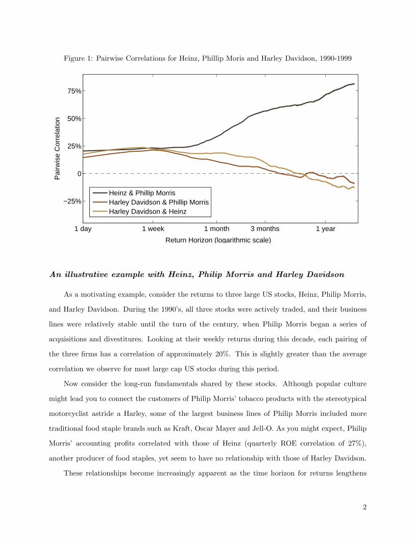
Figure 1: Pairwise Correlations for Heinz, Phillip Moris and Harley Davidson, 1990-1999
1 day 1 week 1 month 3 months 1 year
−25%
0
25%
50%
75%
Return Horizon (logarithmic scale)
Pai
rwis
e C
orre
latio
n
Heinz & Phillip MorrisHarley Davidson & Phillip MorrisHarley Davidson & Heinz
An illustrative example with Heinz, Philip Morris and Harley Davidson
As a motivating example, consider the returns to three large US stocks, Heinz, Philip Morris,
and Harley Davidson. During the 1990’s, all three stocks were actively traded, and their business
lines were relatively stable until the turn of the century, when Philip Morris began a series of
acquisitions and divestitures. Looking at their weekly returns during this decade, each pairing of
the three firms has a correlation of approximately 20%. This is slightly greater than the average
correlation we observe for most large cap US stocks during this period.
Now consider the long-run fundamentals shared by these stocks. Although popular culture
might lead you to connect the customers of Philip Morris’ tobacco products with the stereotypical
motorcyclist astride a Harley, some of the largest business lines of Philip Morris included more
traditional food staple brands such as Kraft, Oscar Mayer and Jell-O. As you might expect, Philip
Morris’ accounting profits correlated with those of Heinz (quarterly ROE correlation of 27%),
another producer of food staples, yet seem to have no relationship with those of Harley Davidson.
These relationships become increasingly apparent as the time horizon for returns lengthens
2

and the estimated correlations differ significantly from the one-week estimates. Figure 1 shows how
the correlation estimates change with the length of the return interval used within the decade. As
the horizon increases, the correlation of the returns of Philip Morris and Heinz steadily increases
to greater than 70%, while the correlations of each firm’s returns with those of Harley Davidson
decrease to approximately zero.
Admittedly, the examples of Heinz, Philip Morris and Harley Davidson are selected ex post
from an enormous number of pairwise correlations and possible sample periods. Estimates of long-
horizon correlations are noisy and the plots in Figure 1 could be coincidental. A more careful
analysis of US stock returns between 1970 and 2010 confirms patterns of this sort are pervasive.
Contributions and connections with related research
A number of researchers have highlighted characteristics that appear to drive excess comove-
ment in equity returns. Barberis, Shleifer, and Wurgler (2005) and Boyer (2011) consider equity
index inclusion and find that the addition of a stock to major market indices causes an immediate
increase in the correlation of its returns with other index constituents. Similarly, Brealey, Cooper,
and Kaplanis (2009) look at changes in exchange listing due to cross-border mergers and find a
stock’s comovement immediately increases with securities listed in its new home market. Con-
trolling even more strongly for differences in fundamental risk, Dabora and Froot (1999) look at
companies with shares that trade on multiple exchanges and find that the prices of otherwise identi-
cal claims diverge from each other and move with other stocks listed on their respective exchanges.
The empirical strategy employed in each of these papers compares comovement in a specific subset
of stocks for which circumstances suggest there are no differences in fundamental risk, at least on
average.
In contrast, my approach examines a broad universe of stock prices and seeks to measure
the aggregate extent to which fads and fundamentals drive comovement. Instead of comparing
correlations immediately before and after some event, I compare correlations made over the exact
same time period where the only difference is the return increment. In this respect, there are fewer
concerns about omitted risks associated with the treatment effect.
The study of excess comovement and fundamentals bears similarity to the work motivated
by Shiller (1981), questioning how the aggregate stock market can be so volatile compared to the
3

relatively stable pattern of dividends received by investors. This led to a large literature testing
variance ratios over various time horizons. There are two advantages to studying correlations rather
than variance ratios. First, correlations control for volatility and are less affected by time variation
in market discount rates. Second, the rich cross section of correlations allows for panel analysis,
avoiding many of the econometric shortcomings associated with analyzing long-horizon returns in
a limited time series.
One of the more striking empirical features of equity correlations is the fact that the historical
correlations between most stocks increase as their return horizon lengthens. This stylized fact has
not gone unnoticed. Campbell, Lettau, Burton, and Xu (2001) study the volatility of individual
equities and note how equity correlations generally declined during the 1980’s and 1990’s and how
correlation estimates using daily returns are, on average, lower than those using monthly returns.
Lo and MacKinlay (1990) study the profitability of contrarian strategies and attribute the success
of this strategy to positive cross-autocorrelation. Their conclusions imply that correlations increase
with time horizon. This is historically true, though I show much of this effect is due to market
microstructure and becomes less prominent as trading costs have decreased.
What sort of labels might be most salient for investors fads? Since market capitalization and
relative valuations are common groupings, we might associate fads with investment styles based on
size and value. This is a key prediction of Barberis and Shleifer (2003), who propose style driven
investing accommodates the cognitive limitations of investors. Veldkamp (2006) derives similar
predictions in a rational setting where investors generalize costly information across similar firms.
My empirical results show weak evidence that firms of a similar size exhibit excess comovement,
and my results do not show excess comovement in firms with similar book-to-market ratios.
Others have connected evidence of excess comovement with trading patterns by obtaining trade
or position data for retail investors (Kumar and Lee, 2006) and mutual fund managers (Greenwood
and Thesmar, 2011; Anton and Polk, 2010). Given the increasing importance of index benchmarks,
Greenwood (2008) looks at how index construction can lead to return patterns induced by index
based trading. In this paper, I attempt to measure shared trading behavior directly by using the
mechanical autocorrelations in returns caused by bid-ask bounce (Roll, 1984) or the temporary
market impact of trading (Campbell, Grossman, and Wang, 1993).
To measure shared fundamentals, my primary measure is the past correlation of accounting
4

returns, measured by return on equity (ROE). I also look at common industry membership as an
indicator that firms face similar demand or profitability shocks. The attempt to connect stock
comovement to fundamentals builds on the work of Pindyck and Rotemberg (1993), who find most
price comovement is unrelated to macroeconomic shocks and Cohen, Polk, and Vuolteenaho (2009),
who find the CAPM performs better when they measure betas using accounting returns rather than
traditional price return betas.
The relationship between return horizon and correlation serves as a valuable measure of excess
comovement in asset prices. It quantifies the economic significance of previous studies that identify
a individual phenomena driving excess comovement. By introducing measures of trading behavior
and fundamentals, I can further identify the fads associated with excess comovement and the
insufficient comovement associated with shared fundamentals. This is a natural framework to
think about risk and portfolio construction, which yields intution for portfolio management and
asset prices.
2 Modeling and Measuring Comovement
To better understand how correlations might change with time horizon, consider what happens
to the comovement of asset prices if investors are slow in incorporating new information about
fundamental value and if swings in the popularity of investments affect their demand. We can
contrast this with the case of no return predictability or where return predictability comes through
long-term time variation in discount rates. This simple model of fads and fundamentals also suggests
a prediction regarding which pairs of assets will show correlations increasing with time horizon and
which pairs of assets will show decreasing correlations.
The model could apply to any sort of financial asset or portfolio of assets. The effect of
time horizon on correlation is likely greatest in cases where markets are segmented or where the
fundamental value is opaque. However, the notation and presentation of the model will consider
the assets to be individual equity securities, in line with the empirical analysis to be presented.
5

Modeling fads and fundamentals
Define the fundamental value of security i at time t as P ∗i,t, entitling its owner to payout Di,t+1.
Changes in log value, ∆p∗i,t+1 = lnP ∗i,t+1+Di,t+1
P ∗i,t
will be a combination of the expected return and
the unexpected shock,
∆p∗i,t+1 = Et[∆p∗i,t+1
]+ ηi,t+1. (1)
Suppose that the market price may differ from this fundamental value for two reasons: first,
transitory fads may cause short-run price deviations across certain groups of securities, and second,
changes in fundamental value may be incorporated with a delay. This can be modeled in a simple
way by defining the log return to security i as
ri,t+1 = ∆p∗i,t+1 −∆di,t+1 + ∆fi,t+1 (2)
where the delay in incorporating fundamentals, ∆di,t+1, is governed by δd ∈ [0, 1) in
∆di,t+1 = ηi,t+1 − (1− δd)∞∑k=0
δkdηi,t−k+1, (3)
and the fad component,
∆fi,t+1 = εi,t+1 −1− δfδf
∞∑k=1
δkfεi,t−k+1, (4)
has shocks εi,t+1 that decay through δf ∈ [0, 1). I will assume that ηi,t and εi,t are independent
martingale difference sequences.
Although this implies predictability in returns, it may not be easy to recognize. These two
forces have offsetting effects on univariate tests of predictability. For example, consider an attempt
to detect forecastability using the autocovariance. For simplicity, we’ll assume for now that expected
returns change very little (i.e. Cov[Et[∆p∗t+1
],Et+τ−1
[∆p∗t+τ
]]≈ 0)2. The autocovariance of rt
2Note that short-term variation could be driven by behavioral or rational causes, but the label ”fad” will be usedto categorized price movement that is transient and over very short horizons. The empirical impact of time variationin discount rates is specifically addressed in section 6.
6
with return rt+τ realized τ > 0 periods in the future is
Cov [rt, rt+τ ] = δτd (Var [ηi,t −∆di,t])︸ ︷︷ ︸momentum in fundamentals
− δτf(δ−1f Var [∆fi,t − εi,t]
)︸ ︷︷ ︸
reversal in fads
. (5)
The delays in incorporating information contribute to momentum in returns (positive autocorre-
lation), but the transient nature of fads contribute to return reversal (negative autocorrelation).
These may offset enough that it is hard for an autocorrelation or variance ratio test to reject the
null hypothesis of no predictability.
Fortunately, we may be able to take advantage of variation in the way fads and fundamentals
affect different assets. In the context of this model, there will be an asset j for which we can measure
the effect of the fad (the correlation of εi,t with εj,t) or delayed fundamentals (the correlation of ηi,t
with ηj,t). A temporary increase in the popularity of blue chip stocks, for example, may cause the
prices of these firms to rise together even when their future earnings are unchanged and unrelated.
Measures of comovement across assets could offer better information regarding the extent to which
prices temporarily deviate from fundamentals.
Defining comovement
To be more precise in defining comovement, I will generally refer to the short-term comovement
of asset i and asset j as their contemporaneous correlation
ρij (1) =Cov [ri,t+1, rj,t+1]√
Var [ri,t+1] Var [rj,t+1]. (6)
The long-horizon return of asset i over H periods will be∑H
h=1 ri,t+h, so the long-term comovement
of asset i and asset j is then the correlation associated with their returns with horizon length H ,
ρij (H) =Cov
[∑Hh=1 ri,t+h,
∑Hh=1 rj,t+h
]√
Var[∑H
h=1 ri,t+h
]Var
[∑Hh=1 rj,t+h
] . (7)
One advantage of measuring comovement through correlations is that it controls for changes in
the variance of assets i and j in the denominator. In that sense we are focusing on their joint
7

price behavior as opposed to factors affecting their individual volatilities. A key result comes from
expanding the variance and covariance terms in the definition of long-term correlation,
Cov
[H∑h=1
ri,t+h,H∑h=1
rj,t+h
]=
H∑h=1
Cov [ri,t+h, rj,t+h] +∑k 6=h
H∑h=1
Cov [ri,t+h, rj,t+k]
Var
[H∑h=1
ri,t+h
]=
H∑h=1
Var [ri,t+h] +∑k 6=h
H∑h=1
Cov [ri,t+h, ri,t+k] . (8)
The assumption of no fads or delayed fundamentals means past returns do not forecast the
future. This implies Cov[ri,t+h, rj,t] = 0 ∀j and ∀h 6= 0, so the double summations in the equations
above must equal zero. In this case
ρij (H) = ρij (1) ∀H , (9)
and correlations should be the same regardless of return horizon. We might denote the difference
between long-run and short-run correlations as ∆ρij = ρij (H) − ρij (1). My null hypothesis is
∆ρ = 0. As an alternative, I propose Cov[ri,t+h, rj,t] 6= 0 and is instead
Cov [ri,t+h, rj,t] = ρτd (Cov [ηi,t −∆di,t,ηj,t −∆dj,t])︸ ︷︷ ︸shared fundamentals
− ρτf(ρ−1f Cov [∆fi,t − εi,t,∆fj,t − εj,t]
)︸ ︷︷ ︸
shared fads
. (10)
This will be positive when the first term is more important for a pair of firms and negative when
the second term dominates. Correlations will no longer remain consistent regardless of time hori-
zon. Instead, equation (??) shows how firms with similar fundamentals will have correlations that
increase with time horizon and firms whose prices share exposure to fads will have correlations that
decrease with time horizon.
Empirical estimation of comovement
Estimating the relationships of long-horizon returns can be problematic within a given sample.
The sample size effectively gets smaller as the return horizon increases. For example, with a return
horizon of six months, a decade of data allows for only twenty independent increments. Additionally,
the long-horizon returns within a given sample will depend on the start and end dates chosen. Six
8

month returns starting in January and June might yield different results than returns starting in
April and October. We can minimize the impact of these limitations by estimating correlations
using every possible overlapping window available.
Within a given sample, a correlation for horizon length H is estimated as
ρij (H) =
∑Hh=−H
(H−hH
)cij (h)√(∑H
h=−H(H−hH
)cii (h)
)(∑Hh=−H
(H−hH
)cjj (h)
) . (11)
The empirical cross-autocovariance cij (h) measures the relationship between ri and rj ’s realizations
of h periods in the future,
cij (h) =1
H − r∑
(ri,t − ri) (rj,t+r − ri) . (12)
Estimating long-run correlations using (11) is equivalent to averaging the correlation estimates
for returns of horizon length H using all possible windows. Suggestively, this is also identical to the
correlation resulting from Newey and West’s (1987) estimator of the long-run covariance of a time
series. The fundamental risk in a financial time series is closely related to the concept of long-run
variance, which continues to be a major topic of research in time series econometrics.
The price impact of trading behavior
To identify the sorts of firms whose prices are driven by shared trading behavior rather than
fundamentals, we could propose characteristics that might be overly salient to investors and test
to see if they predict negative values for ∆ρij . For example, if investment styles are indicative of
non-fundamental related trading they would show negative coefficients in a regression.
To capture trading behavior more directly, we can try to measure which assets tend to be
contemporaneously bought and sold. The simple model above would predict that assets with a
greater degree of shared trading behavior will exhibit more values for ∆ρij . While it might seem
difficult to observe data on who is initiating transactions, I will show how shared trading behavior
can be inferred by looking at correlations in bid-ask bounce.
Consider Roll’s (1984) model of the effective bid-ask spread. He notes that the closing price
recorded for a security can be affected by whether the last trade was driven by a purchase or a sale.
9

This price differential can be interpreted as the literal bid-ask spread paid by buyers and sellers
who initiate trades with market makers, or this could be a more modern concept of temporary price
impact as the intensity of buying or selling pressure affects liquidity provision.
Suppose that an average sized buyer must pay pi,t + bi, and sellers of an average quantity
receive pi,t − bi. Hence bi can be thought of as the temporary market impact of trading. Any
permanent impact from information in trades is captured by updates in pi,t. The observed return
is then a combination of the price change and the transitory market impact of purchases (indicated
by binary variable ηi,t = 1) or sales (when ηi,t = −1). The observed return (ri,t+1) can be expressed
as the log return (ri,t+1 = pi,t+1 − pi,t) plus the market impact
ri,t+1 = ri,t+1 + bi (ηi,t+1 − ηi,t) . (13)
Let’s assume that purchases and sales are equally likely and are independent each period and the
null hypothesis that past price changes are not predictive of the future. The effect of this trading
on the autocovariance sequence for returns will be
Cov [ri,t, ri,t] = Var [pi,t+1 − pi,t+1] + b2i
Cov [ri,t, ri,t+1] = −b2i
Cov [ri,t, ri,t+k] = 0 ∀k > 1. (14)
This is precisely what motivated Roll’s estimate of the effective bid-ask spread:
bi = −√
Cov [ri,t, ri,t+1]. (15)
And what if the buying pressure is correlated across firms? Suppose that investors tend to
buy and sell asset i and asset j at the same time, so that νij = E[ηi,t, ηj,t] 6= 0. We would observe
νij > 0 if the trading behavior is similar and νij < 0 if investors tend to buy one while selling the
other. Intuitively, we can write νij as a simple function of the probability that securities are both
10
exposed to common trading behavior,
νij = 2× (Pr [ηi,t = ηj,t]− 0.5) . (16)
This is the proposed measure of common trading behavior. Just as we can measure the
effective bid-ask from the autocovariances, we can estimate common trading behavior from the
cross-autocovariances. Under the same assumptions as above, they will be
Cov [ri,t, rj,t] = Cov [ri,t+1, rj,t+1] + 2νijbibj
Cov [ri,t, rj,t+1] = −νijbibj (17)
Cov [ri,t, rj,t+k] = 0 ∀k > 1.
From this, I empirically estimate this measure νij of how trading behavior connects two stocks
through
νij = − Cov [ri,t, rj,t+1] + Cov [ri,t+1, rj,t]
2√
Cov [ri,t, rj,t+1] Cov [ri,t, rj,t+1]. (18)
3 Short-Run and Long-Run Comovement in US Equities
Data sources and variable construction
To estimate the comovement of US equity prices, I use four decades of weekly total returns
from The Center for Research in Security Prices3 (CRSP), covering the forty years from 1970 to
2009, and each decade is considered a subsample. To ensure the analysis focuses on the most
liquid securities, I select the 2,000 largest issues by market cap as determined immediately prior to
the start of each decade. The weekly log returns are measured using Tuesday’s closing prices and
include any distributions received. For the most recent decade spanning 2000-2009, the universe
consists of the largest 2,000 firms measured by their market cap on December 31st, 1999, and the
first weekly return is measured from January 4th to January 11th, 2000. Only publicly traded
common stock of US incorporated firms are considered (CRSP share codes 10 and 11).
3Center for Research in Security Prices. c©2011 Booth School of Business, The University of Chicago. Used withpermission. All rights reserved. www.crsp.chicagobooth.edu
11

Within each decade, short-run and long-run correlations are calculated for every pair of firms,
where the short run is defined as one week and the long run is defined as half of a year. Short-run
correlations of weekly returns, ρ (1) are calculated as in (6). The long-run correlation calculation
uses the formula in (7) where H = 26 weeks, generating ρ (26). The difference between the two
yields ∆ρ.
To minimize any bias related to survivorship, long-run correlations are calculated whenever
possible, even when two firms coexist for only a small portion of the decade. The minimum possible
number of observations to calculate ρ (26) is approximately one year. The trade-off for reducing
this bias is sampling variance, as the long-run variance in those cases is exceptionally noisy. In
practice, requiring a longer minimum history decreases the sample size and affects the results very
little, so I make this criterion as permissive as possible.
We can be reasonably comfortable that the results of the empirical analysis are not driven by
the anomalous behavior of illiquid firms since the universe consists of the largest 2,000 securities by
market capitalization and the shortest time interval considered is one week. The mean difference
between short-run and long-run correlation increases when using smaller firms and shorter time
horizons, and there is also a slight increase in the predictability of this difference, but these results
are excluded as they would be open to criticism that they are affected to a larger extent by stale
prices or other liquidity related issues.
Summarizing the correlations over long and short horizons
Summary statistics for the correlation estimates are shown in Table 1. The sample size of
2,000 firms will generate slightly less than two million correlation unique correlation estimates each
decade. The first panel shows the effect of attrition on data coverage. You can see that correlations
can be calculated for more than 90% of all possible pairs of firms except in the most recent decade
where the ten-year period begins in the year 2000, at the peak of the Internet frenzy. Acquisitions
and failures cause an atypical number of firms to disappear during the first 12 months of this
subsample.
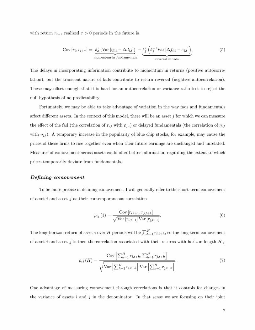
For the four decades considered, the short-run correlation, ρij (1), averages 18.4%, with a
standard deviation of 11.4%. In contrast, long-run correlations are much higher, with a full sample
average of 30.0% and standard deviation of 27.0%. The difference between the two, ρ (H)− ρij (1),
12
Table 1: Data Coverage and Summary Statistics for Correlation Estimates
This table reports the data availability and summary statistics for the estimated return correlations. The return seriesconsidered are log returns calculated from the CRSP total return data, and the minimum unit of measurement is oneweek, corresponding to returns from Tuesday to Tuesday. The short run correlation measures, ρ (1), are thereforeassociated with a one week horizon. In the data panel measuring coverage by unique correlation pairs, the uniquecorrelation estimates correspond to the upper triangle of the matrix of correlation coefficients, excluding the diagonal.
Coverage
by unique correlation pairs Decade Full Sample1970’s 1980’s 1990’s 2000’s
max possible pairs 1,999,000 1,999,000 1,999,000 1,999,000 7,996,000pairs w/ min # returns 1,872,110 1,811,088 1,828,826 1,632,793 7,144,817
Summary Statistics
short-horizon correlation Decade Full Sample1970’s 1980’s 1990’s 2000’s
mean 22.81 19.20 13.01 18.31 18.36std dev 9.12 10.55 9.31 13.90 11.36
ρij(1) 5 %ile 8.55 2.59 -0.90 -5.16 0.53median 22.57 18.96 12.43 18.53 18.1895 %ile 37.84 36.74 28.88 40.73 36.96
long-horizon correlation Decade Full Sample1970’s 1980’s 1990’s 2000’s
mean 45.12 30.03 22.77 20.72 30.00std dev 19.98 24.79 24.84 30.65 26.94
ρij(26) 5 %ile 10.52 -15.72 -18.44 -37.30 -18.62median 46.69 32.80 23.06 24.26 32.8795 %ile 74.95 65.68 63.59 64.71 68.81
correlation difference Decade Full Sample1970’s 1980’s 1990’s 2000’s
mean 22.31 10.83 9.76 2.42 11.64std dev 18.36 22.21 22.73 26.23 23.52
∆ρij 5 %ile -9.37 -28.15 -27.77 -45.68 -29.86median 23.70 12.30 10.01 4.91 13.5595 %ile 49.47 44.63 46.79 40.93 46.43
13

averages 11.6%. The difference decreases over time, with an average difference of 22.3% in the
1970’s decreasing to a difference of only 2.4% in the most recent decade.
By definition, there are upper and lower bounds on the possible observed correlations. In
practice, the estimated short-run correlations are nearly always positive, with less than 5% of the
estimated values being less than zero. However, there is much more variation in the long horizon
correlation estimates. Even though the average long-run correlation is nearly twice as large, a little
less than a third of the estimates are less than zero.
While the standard deviations and percentiles shown in Table 1 make it tempting to conclude
that there is a larger degree of cross-sectional variation in correlations measured over long horizons,
it is important to note that the short-run correlations are estimated much more precisely. Even
under the null hypothesis where the true correlation does not depend on the time horizon, the
empirical long-run correlations will show more variation due to the fact that they are estimated
using far fewer independent observations. We cannot yet draw conclusions about the distribution
of the true long-run correlations. The full sample standard deviation of 27.0% reflects both the
dispersion of correlations in the population as well as the measurement error. Section 4.2 will
present how a method for quantifying the effect of measurement error in the long run estimates.
4 A Regression Methodology for Correlations
Regressing explanatory variables on the correlation differences
To test the null hypothesis in (9) against the alternative, I propose running a regression of
the difference in long-run and short-run correlation on candidate explanatory variables for each
pair of firms. Negative values for this difference in correlations correspond to excess comovement,
indicating the pair of stocks has a higher correlation in the short run than can be justified by their
long-run returns. Positive values are indicative of insufficient comovement, as the short-run returns
do not seem to capture the comovement observed over longer horizons.
Given explanatory variables corresponding to each pair of firms (i, j) whose shared character-
istics constitute vector Zij (including a constant term), the coefficient vector β is estimated from
the linear regression
∆ρij = βZij + eij . (19)
14

Under the null hypothesis, every element of β, including the constant, is equal to zero.
Calculating the standard errors for β requires special attention, since these errors are not inde-
pendent across pairs of firms. The traditional standard errors estimated using an OLS regression to
estimate (19) will be far too small. What appears to be a large cross-sectional sample is effectively
smaller since much of the variation in stock returns is driven by common factors. Even worse, all
stocks likely have a positive loading on a single factor, the market. If none of the residuals are
independent, traditional techniques to handle correlated residuals in a cross-sectional regression,
like clustering standard errors, will offer little help.
A reshuffling technique for statistical inference
The problem would benefit from a new approach. Note that under the null hypothesis, this
error term eij is equal to the estimation error between the true long-horizon correlation and whatever
empirical estimate results from the particular sample used. We can call this estimation error
εij = ∆ρij −∆ρij (H) , (20)
and note that eij = εij , under the null hypothesis.
Fortunately we can take advantage of some properties of the null hypothesis. In particular,
the assumption of no predictability suggests that the error terms in (20) result from the purely
coincidental estimation noise of past returns appearing to predict the future.
Therefore, the historical ordering of the weekly returns makes no difference. We just need
to preserve the contemporaneous return structure. In fact, if we randomly reshuffle the historical
ordering of the weeks and recalculate the long-run correlations, we would generate an independent
draw of error terms with the same statistical properties.
This is effectively what I propose as a robust, non-parametric for calculating standard errors.
With new long-term correlation estimates from each reshuffling of the weekly returns, we find the
distribution of β under the null by repeatedly rerunning the regression in (19). Then we can
compare our β estimate to the distribution of estimates generated from the reshuffled data. We
can now test the hypothesis that β = 0 properly accounting for the strong dependence across our
observations.
15
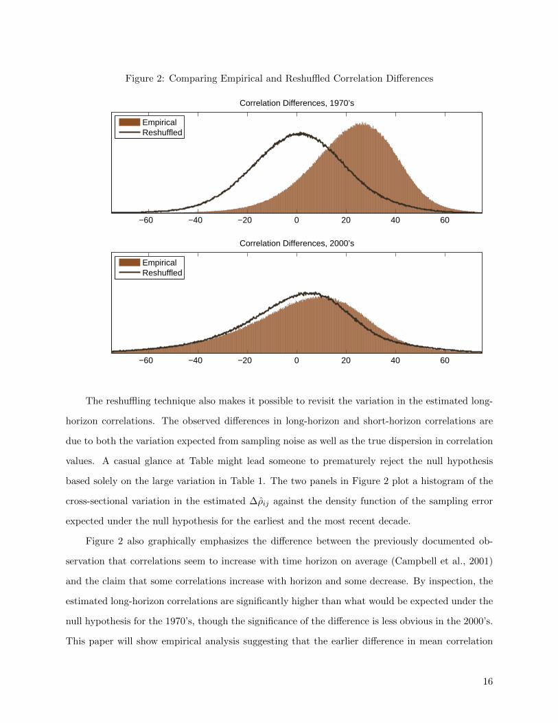
Figure 2: Comparing Empirical and Reshuffled Correlation Differences
−60 −40 −20 0 20 40 60
Correlation Differences, 1970’s
−60 −40 −20 0 20 40 60
Correlation Differences, 2000’s
EmpiricalReshuffled
EmpiricalReshuffled
The reshuffling technique also makes it possible to revisit the variation in the estimated long-
horizon correlations. The observed differences in long-horizon and short-horizon correlations are
due to both the variation expected from sampling noise as well as the true dispersion in correlation
values. A casual glance at Table might lead someone to prematurely reject the null hypothesis
based solely on the large variation in Table 1. The two panels in Figure 2 plot a histogram of the
cross-sectional variation in the estimated ∆ρij against the density function of the sampling error
expected under the null hypothesis for the earliest and the most recent decade.
Figure 2 also graphically emphasizes the difference between the previously documented ob-
servation that correlations seem to increase with time horizon on average (Campbell et al., 2001)
and the claim that some correlations increase with horizon and some decrease. By inspection, the
estimated long-horizon correlations are significantly higher than what would be expected under the
null hypothesis for the 1970’s, though the significance of the difference is less obvious in the 2000’s.
This paper will show empirical analysis suggesting that the earlier difference in mean correlation
16
differences can be largely attributed to microstructure noise from the bid-ask spread.
Setting aside differences in the mean, the dispersion in the reshuffled values is quite high,
suggesting that we cannot immediately rule out the possibility that large cross-sectional differences
in correlation estimates for different time horizons are simply sampling error. A more careful
analysis will show evidence that correlations will predictably increase or decrease as the return
horizon lengthens.
5 Explaining Empirical Correlations
Data description of explanatory variables
All of the explanatory variables that form the elements of the Zij vector of explanatory variables
in estimating (19) are calculated using data available prior to each decade. I group them by factors
ostensibly related to investment behavior and factors that are indicative of shared fundamental
risks.
I estimate shared trading behavior by calculating the correlations in bid-ask bounce, νij , as
defined in (18). Log weekly returns are used to estimate νij using a two year window prior to
the start of the decade. The effective bid/ask spread, used in the denominator of the definition of
shared trading behavior is shrunk toward the median value estimated across all securities, which
prevents a negative implied spread in most cases. To further control for large outliers that may be
driven by a very small denominator, or by estimation error in the numerator, the final values of νij
are all shrunk toward zero.
Somewhat surprisingly, Table 2 shows that, on average, firms do not tend to be bought and
sold together for the first two decades in the sample. This might be indicative that the trading
behavior tended to reflect investors shifting investments across stocks rather than a pattern of
broad net inflows or outflows in the equity market. For the more recent two decades, however, the
mean coefficient is much closer to zero and shows no particular propensity for stocks to be bought
or sold together, though this varies significantly across pairs of stocks.
My primary measure to estimate fundamental correlation is the correlation of firms’ return
on equity. ROE values are constructed from Compustat data, defined as the ratio of earnings per
17
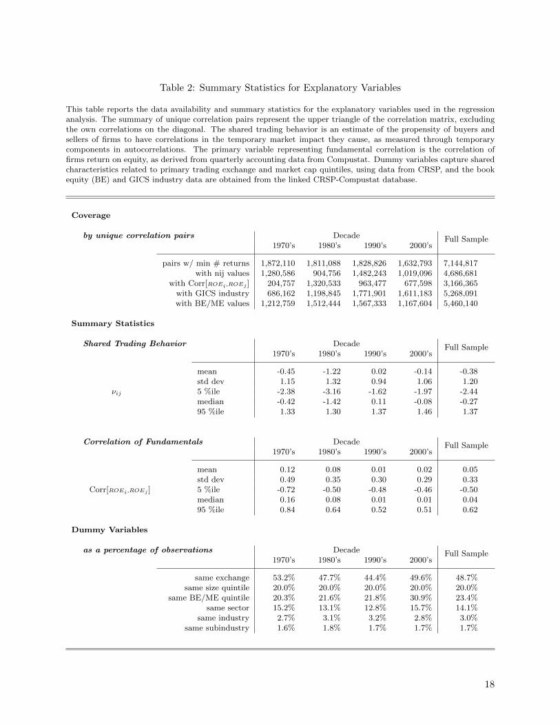
Table 2: Summary Statistics for Explanatory Variables
This table reports the data availability and summary statistics for the explanatory variables used in the regressionanalysis. The summary of unique correlation pairs represent the upper triangle of the correlation matrix, excludingthe own correlations on the diagonal. The shared trading behavior is an estimate of the propensity of buyers andsellers of firms to have correlations in the temporary market impact they cause, as measured through temporarycomponents in autocorrelations. The primary variable representing fundamental correlation is the correlation offirms return on equity, as derived from quarterly accounting data from Compustat. Dummy variables capture sharedcharacteristics related to primary trading exchange and market cap quintiles, using data from CRSP, and the bookequity (BE) and GICS industry data are obtained from the linked CRSP-Compustat database.
Coverage
by unique correlation pairs Decade Full Sample1970’s 1980’s 1990’s 2000’s
pairs w/ min # returns 1,872,110 1,811,088 1,828,826 1,632,793 7,144,817with nij values 1,280,586 904,756 1,482,243 1,019,096 4,686,681
with Corr[ROEi,ROEj ] 204,757 1,320,533 963,477 677,598 3,166,365with GICS industry 686,162 1,198,845 1,771,901 1,611,183 5,268,091with BE/ME values 1,212,759 1,512,444 1,567,333 1,167,604 5,460,140
Summary Statistics
Shared Trading Behavior Decade Full Sample1970’s 1980’s 1990’s 2000’s
mean -0.45 -1.22 0.02 -0.14 -0.38std dev 1.15 1.32 0.94 1.06 1.20
νij 5 %ile -2.38 -3.16 -1.62 -1.97 -2.44median -0.42 -1.42 0.11 -0.08 -0.2795 %ile 1.33 1.30 1.37 1.46 1.37
Correlation of Fundamentals Decade Full Sample1970’s 1980’s 1990’s 2000’s
mean 0.12 0.08 0.01 0.02 0.05std dev 0.49 0.35 0.30 0.29 0.33
Corr[ROEi,ROEj ] 5 %ile -0.72 -0.50 -0.48 -0.46 -0.50median 0.16 0.08 0.01 0.01 0.0495 %ile 0.84 0.64 0.52 0.51 0.62
Dummy Variables
as a percentage of observations Decade Full Sample1970’s 1980’s 1990’s 2000’s
same exchange 53.2% 47.7% 44.4% 49.6% 48.7%same size quintile 20.0% 20.0% 20.0% 20.0% 20.0%
same BE/ME quintile 20.3% 21.6% 21.8% 30.9% 23.4%same sector 15.2% 13.1% 12.8% 15.7% 14.1%
same industry 2.7% 3.1% 3.2% 2.8% 3.0%same subindustry 1.6% 1.8% 1.7% 1.7% 1.7%
18

share (Compustat item: epspiq) divided by common equity per share (Compustat item: ceqq). This
value is censored at -90% and +100% and then converted to a log return. Annual Compustat data
is used to supplement where quarterly data is not available. Correlations in this ROE series are
calculated for each pair of firms over the prior 10 years, excluding the quarter immediately prior
to the beginning of the decade, since this data is typically not released until January or later. I set
a minimum requirement of 4 years of accounting data to estimate a valid correlation. As can be
seen in the coverage statistics in Table 2, lack of Compustat data tends to be the most restrictive
data requirement, especially near the beginning of the sample when only a few hundred firms have
accounting data available. This does not have a substantive effect on the regression results, but I
will run a regression specification that excludes Corr[ROEi,ROEj ] to take advantage of the larger
data set.
Market cap and exchange information all come from CRSP, and the book equity and GICS
industry assignments are all taken from the CRSP-Compustat linked database. The construction
of the book equity / market equity (BE/ME) variable mirrors that described by Fama and French
(1992). Each decade, the 2000 firms in the universe are matched to their assigned to BE/ME
quintiles relative to the CRSP universe of firms. I do not use the CRSP universe for market
cap quintile assignments, since my sample of the 2,000 largest firms only represents the largest
quintiles. Instead, I create market cap quintiles specific to this sample using market cap data from
the December previous to the start of each decade.
This information allows for the construction of the dummy variables shown in Table 2. They
correspond to pairs of firms being listed on the same exchange, sharing the same size quintile,
being assigned the same GICS industry, etc. As usual, the dummy variables equal 1 for each
pairwise observation where the criteria are met. The classifications of sharing the same GICS
sector, industry or subindustry are not exclusive of each other, so a pair of firms in the same
subindustry will necessarily also be in the same industry and sector. The occurrence of firms in
the same subindustry is the rarest of the dummy variables, occurring in about 1.7% of the unique
firm pairs, but will be shown to have a strong effect even after controlling for industry and sector.
19

Regressing explanatory variables on ∆ρ
Following the methods described in section 4, I estimate regression coefficients for each decade
subsample via least squares and use the reshuffling technique to calculate standard errors. The
regression estimates for regressions of ∆ρ on various explanatory variables are combined (assuming
independent subsamples) and reported in Table 3.
The first regression specification includes no explanatory variables other than constant terms.
While these regression coefficients are going to reflect the simple means previously noted in the
summary statistics, the reshuffling methodology help us better understand the significance of these
results. We can see that even across almost 2 million observations per decade, the common factors
driving returns can generate standard errors in the average difference in long-run and short-run
correlations of about 3%. The fact that long-horizon correlations average 2.42% higher than short-
horizon correlations in the most recent decade is well within the range of differences we might
randomly observe. The differences in earlier decades, as large as 22% during the 1970’s, cannot be
explained by estimation error.
The second regression specification includes the two primary explanatory variables reflecting
shared trading behavior (νij) and shared fundamentals (Corr[ROEi, ROEj ] ). Both of these vari-
ables are highly significant in explaining the effect of return horizon on correlations. As expected,
common trading behavior is indicative of temporary price comovement, as indicated by the nega-
tive coefficient. Firms that have a higher probability of being bought or sold together have higher
short-horizon correlations but lower correlations over long horizons. The variable measuring shared
fundamentals generates a positive regression coefficient and the opposite effect of trading behav-
ior. Firms with highly similar fundamental exposures tend to have lower short-horizon correlations
relative to long horizons, suggesting insufficient comovement.
The third regression specification adds the dummy variables indicating firms are traded on the
same exchange, and in similar size or valuation categories, or belong to the same GICS industry
categories. Trading on the same exchange is indicative of excess comovement, consistent with the
international evidence that exchange listings matter. Considering the three principal exchanges on
which these stocks are listed (NYSE, AMEX, and NASDAQ), more than 1% of stock price variation
is associated with temporary comovement with other stocks on the same exchange. As is true with
20
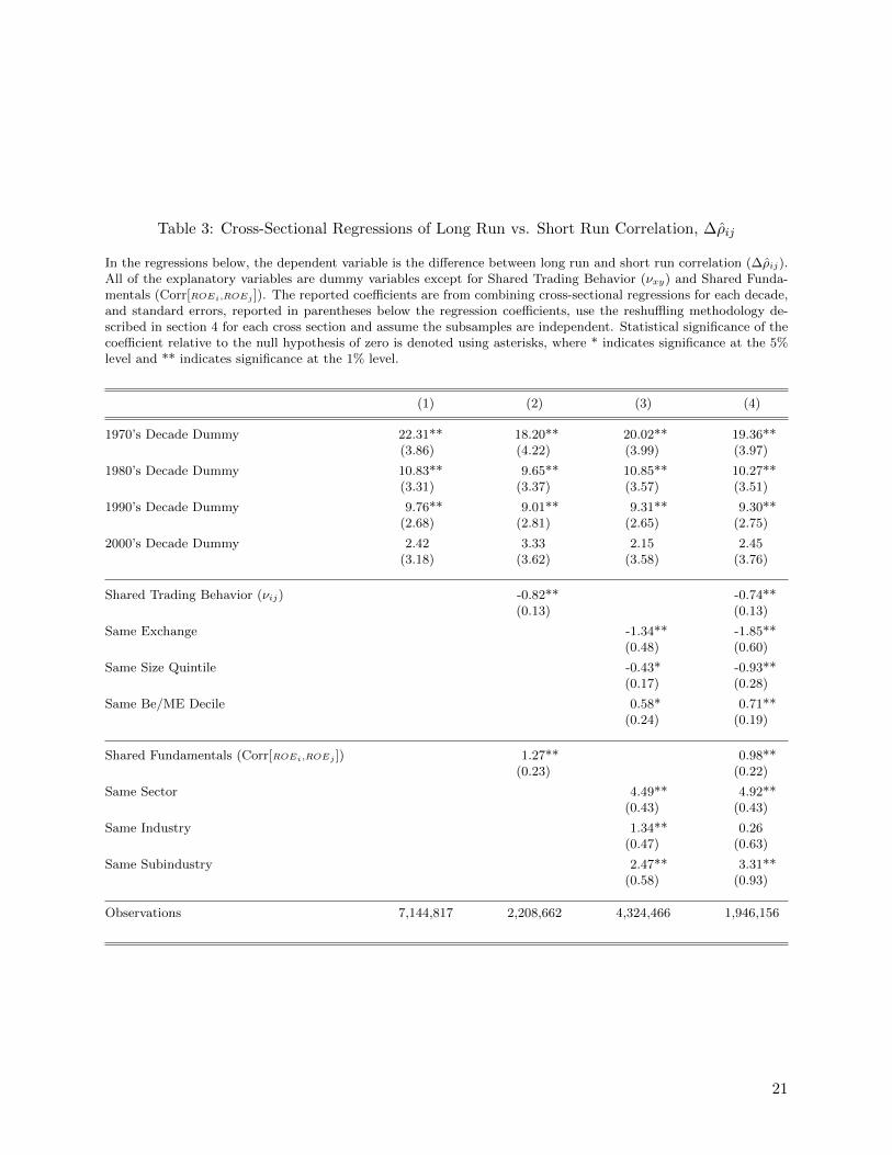
Table 3: Cross-Sectional Regressions of Long Run vs. Short Run Correlation, ∆ρij
In the regressions below, the dependent variable is the difference between long run and short run correlation (∆ρij).All of the explanatory variables are dummy variables except for Shared Trading Behavior (νxy) and Shared Funda-mentals (Corr[ROEi,ROEj ]). The reported coefficients are from combining cross-sectional regressions for each decade,and standard errors, reported in parentheses below the regression coefficients, use the reshuffling methodology de-scribed in section 4 for each cross section and assume the subsamples are independent. Statistical significance of thecoefficient relative to the null hypothesis of zero is denoted using asterisks, where * indicates significance at the 5%level and ** indicates significance at the 1% level.
(1) (2) (3) (4)
1970’s Decade Dummy 22.31** 18.20** 20.02** 19.36**(3.86) (4.22) (3.99) (3.97)
1980’s Decade Dummy 10.83** 9.65** 10.85** 10.27**(3.31) (3.37) (3.57) (3.51)
1990’s Decade Dummy 9.76** 9.01** 9.31** 9.30**(2.68) (2.81) (2.65) (2.75)
2000’s Decade Dummy 2.42 3.33 2.15 2.45(3.18) (3.62) (3.58) (3.76)
Shared Trading Behavior (νij) -0.82** -0.74**(0.13) (0.13)
Same Exchange -1.34** -1.85**(0.48) (0.60)
Same Size Quintile -0.43* -0.93**(0.17) (0.28)
Same Be/ME Decile 0.58* 0.71**(0.24) (0.19)
Shared Fundamentals (Corr[ROEi,ROEj ]) 1.27** 0.98**(0.23) (0.22)
Same Sector 4.49** 4.92**(0.43) (0.43)
Same Industry 1.34** 0.26(0.47) (0.63)
Same Subindustry 2.47** 3.31**(0.58) (0.93)
Observations 7,144,817 2,208,662 4,324,466 1,946,156
21

all the explanatory variables considered, the exchange listing may not be the causal force driving
excess comovement, but it is predictive.
The dummy variable indicating firms are in the same size quintile also has the expected sign.
Prices of firms with similar market caps seem to move together over short horizons much more than
over longer return horizons. On the other hand, the same logic would suggest a negative regression
coefficient on the dummy variable indicating firms are in the same BE/ME quintile, but this is not
the case. The coefficient on this variable is positive. A closer examination of excess comovement
across subsamples and controlling for autocorrelations from market microstructure suggests the
value results are not robust and the size effect is be driven by excess comovement in the firms at
the smaller range of this sample.
The variables indicating firms share the same sector, industry or subindustry all show large
positive coefficients. As with the measure of shared fundamentals that looks at correlations in
profitability, these variables seem to indicate firms with similar factors driving their profitability
show insufficient price comovement over short horizons. For firms in the same subindustry, the
correlation of their 6-month returns will, on average, be 8.3% higher than the correlation of their
weekly returns. This is one of the strongest statistical results, though it’s not without precedent.
Cohen and Frazzini (2008) and Moskowitz and Grinblatt (1999) show evidence of evidence of
positive momentum across connected firms, which would cause their correlations to increase with
the time horizon.
The fourth regression specification includes all explanatory variables. This serves as a check
that each makes an independent contribution. There is a slight decrease in the coefficients on
the main variables measuring shared trading behavior and shared fundamentals, but they remain
highly significant.
Interestingly, the coefficients on the other variables intended to capture labels that might be
salient to investors all increase. The coefficient on firms that share the same size quintile almost
doubles, indicating that it might be more prominent conditioned on the other explanatory variables
than it is when measured in isolation.
The variables intended to capture common exposures to fundamental risks all remain significant
predictors of insufficient short-run comovement with the exception of the dummy variable for firms
sharing the same industry. This is actually an artifact of this measure being so similar to the
22

subindustry dummy variable that the coefficient shifts from one to the other.
The general conclusions from the empirical results are broadly consistent across regression
specifications. They provide evidence in favor of the hypothesis that short-run comovement is
different than long-run comovement, and that excess and insufficient comovement can be predicted
by measures of shared trading behavior and exposures to shared fundamentals.
6 Robustness
The key results in Table 3 are robust across a variety of alternative estimation approaches.
However, there are two critiques that deserve special attention, which I’ll call the ”micro explana-
tion” and the ”macro explanation.” The micro explanation would assert that the correlation differ-
ences are the result of bid-ask spreads and similar effects in market microstructure, and the macro
explanation would assert that correlation differences are simply a manifestation of predictability in
well-known risk factors.
Micro explanation: serial correlations
Just as the bid-ask bounce can be used to estimate trade-driven price behavior, serial correla-
tion from market microstructure can also affect correlations. This is clear from the effects derived
in (14) and (17). In general, long-run correlations will appear mechanically higher than short-run
correlations simply because the temporary price impact of trading constitutes a much smaller frac-
tion of total price movement in long-horizon returns relative to short-horizon returns. Since this
effect will be larger for stocks that are less liquid, the regression analysis might mistakenly associate
measures correlated with liquidity as indicators of insufficient comovement.
To show this is not the source of the results in Table 3, I construct a measure that adjusts the
difference between long and short-horizon correlations that excludes the first order autocorrelation
and cross-autocorrelation terms that could be affected by the impact of trading on closing prices.
I label this variable ∆ρij . These excluded first order autocorrelations would also contain a large
degree of information about excess comovement, so it is important to recognize that assuming them
to be zero may be a useful robustness check, but it biases all results in favor of the null hypothesis.
23

Table 4: Summary Statistics for Microstructure Robust Correlation Differences
This table reports summary statistics for the microstructure robust correlations differences constructed by calculatingthe correlation difference ∆ρij where the autocorrelation terms in defining the long run correlation are assumed tobe zero. The calculations are otherwise identical to those described for ∆ρij .
microstructure adjusted difference Decade Full Sample1970’s 1980’s 1990’s 2000’s
mean 9.30 1.71 5.01 1.74 4.55std dev 16.13 37.68 19.14 32.59 27.83
∆ρij 5 %ile -16.74 -34.49 -25.64 -45.47 -30.07median 9.75 3.03 5.06 4.67 5.9695 %ile 33.92 35.54 35.53 38.10 35.60
Table 4 reports summary statistics for ∆ρij . Comparing these microstructure adjusted esti-
mates to the original summary statistics reported in Table 1. The most striking difference is that
the mean short-run correlation is much closer to the mean long-run correlation. This suggests that
the lower comovement in the short run is driven, in a large part, by the idiosyncratic price impact
from trading that immediately reverses in the subsequent period. This is in line with the predicted
effect of market microstructure.
Not surprisingly, the microstructure adjustments become less significant over time, which is
likely a result of increased liquidity and tighter bid-ask spreads. The dispersion of the difference
remains high on average and over time, suggesting that the return horizon may have a large effect
on individual correlations, even when the difference is only slightly positive in the cross section.
To check the robustness of the regression results directly, I run the previous regressions on ∆ρ,
the difference in long-term and short-term correlations that have been adjusted for microstructure.
These regression results are shown in Table 5.
Adjusting for microstructure effects by regressing on ∆ρ
The most noticeable differences are in the unconditional averages, as seen in the first regression
specification with no other explanatory variables. As was observed in the summary statistics, the
differences all decrease. Looking at the statistical significance only the 9.3% average difference in
the 1970’s remains statistically different from zero at the 5% confidence level. This is consistent
with the idea that a great degree of the insufficient comovement we observed was an artifact of
24

Table 5: Cross-Sectional Regressions Adjusted for Microstructure Effects, ∆ρij
In the regressions below, the dependent variable is the difference between long run and short run correlation, afteradjusting for the first order autocorrelation that is likely caused by bid-ask bounce and other microstructure effects,yielding (∆ρij). All of the explanatory variables are dummy variables except for Shared Trading Behavior (νxy) andShared Fundamentals (Corr[ROEi,ROEj ]). The reported coefficients are from combining cross-sectional regressionsfor each decade, and standard errors, reported in parentheses below the regression coefficients, use the reshufflingmethodology described in section 4 for each cross section and assume the subsamples are independent. Statisticalsignificance of the coefficient relative to the null hypothesis of zero is denoted using asterisks, where * indicatessignificance at the 5% level and ** indicates significance at the 1% level.
(1) (2) (3) (4)
1970’s Decade Dummy 9.30* 6.70 6.95 6.62(3.86) (4.22) (3.99) (3.97)
1980’s Decade Dummy 1.71 1.03 2.33 1.97(3.31) (3.37) (3.57) (3.51)
1990’s Decade Dummy 5.01 4.95 4.61 4.72(2.68) (2.81) (2.65) (2.75)
2000’s Decade Dummy 1.74 4.97 3.94 5.22(3.18) (3.62) (3.58) (3.76)
Shared Trading Behavior (νij) -0.24 -0.21(0.13) (0.13)
Same Exchange -0.70 -0.89(0.48) (0.60)
Same Size Quintile -0.07 -0.13(0.17) (0.28)
Same Be/ME Decile 0.13 0.26(0.24) (0.19)
Shared Fundamentals (Corr[ROEi,ROEj ]) 0.94** 0.56*(0.23) (0.22)
Same Sector 1.61** 1.83*(0.43) (0.43)
Same Industry 0.90 0.04(0.47) (0.63)
Same Subindustry 1.20* 1.50(0.58) (0.93)
Observations 7,144,817 2,208,662 4,324,466 1,946,156
25

temporary impact of trades on closing prices.
Although none of the explanatory variables identified as significant in the prior regression
change drastically, most of their effects are more muted. For example, in the second regression
specification the coefficient on the shared trading behavior variable previously had a coefficient of
-0.82 and a t-statistic of -6.4, but this now drops to a coefficient of -0.24 and an associated t-statistic
of -1.83. It might be that much of the temporary impact captured by this variable corrects itself
in the subsequent week, which is excluded in the calculation of ∆ρ, or it may be that the shared
trading behavior variable also proxies for liquidity.
The other main explanatory variable, measuring correlation in shared fundamentals, sees a
much more moderate decrease in magnitude after adjusting for microstructure and also remains
highly statistically significant. Its coefficient drops from 1.27 to 0.94.
In the fourth regression specification on Table 5 where all explanatory variables are included,
the coefficients are generally smaller than they were in Table 3. The only dummy variable that
could be considered statistically different from zero with greater than 95% confidence is the measure
of firms being in the same GICS sector.
Macro explanations due to discount rates
The assumption that long-horizon and short-horizon correlations should be equivalent comes
from equation (??) where past returns are assumed not to predict the future. No arbitrage as-
sumptions in asset pricing theory suggest that this should be true for conditional moments, but not
necessarily true for unconditional measures of volatility and correlation. Cochrane (1991) empha-
sizes this point, showing how unconditional return predictability does not reject rational pricing
models outright and are exactly what we could expect to see in macroeconomic models where
discount rates vary over time due to changing growth prospects or risk preferences.
The same principle holds true in our analysis. Our null hypothesis would be rejected by a broad
class of models that generate time variation in the price of equity risk. Let’s consider what we would
expect to see in a standard model of this type. In a one-factor model where the expected returns
to stocks are driven by their exposures to the aggregate stock market, time variation in expected
market returns would imply that some of the short-horizon price correlation between stocks is driven
by their common exposure to changes in aggregate return expectations. This common component
26
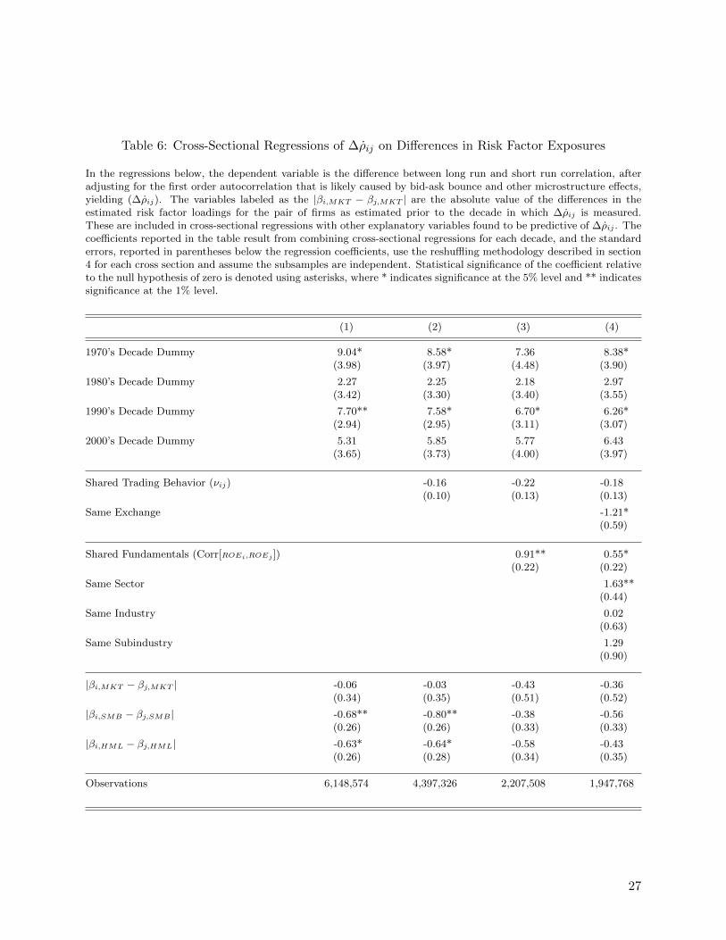
Table 6: Cross-Sectional Regressions of ∆ρij on Differences in Risk Factor Exposures
In the regressions below, the dependent variable is the difference between long run and short run correlation, afteradjusting for the first order autocorrelation that is likely caused by bid-ask bounce and other microstructure effects,yielding (∆ρij). The variables labeled as the |βi,MKT − βj,MKT | are the absolute value of the differences in theestimated risk factor loadings for the pair of firms as estimated prior to the decade in which ∆ρij is measured.These are included in cross-sectional regressions with other explanatory variables found to be predictive of ∆ρij . Thecoefficients reported in the table result from combining cross-sectional regressions for each decade, and the standarderrors, reported in parentheses below the regression coefficients, use the reshuffling methodology described in section4 for each cross section and assume the subsamples are independent. Statistical significance of the coefficient relativeto the null hypothesis of zero is denoted using asterisks, where * indicates significance at the 5% level and ** indicatessignificance at the 1% level.
(1) (2) (3) (4)
1970’s Decade Dummy 9.04* 8.58* 7.36 8.38*(3.98) (3.97) (4.48) (3.90)
1980’s Decade Dummy 2.27 2.25 2.18 2.97(3.42) (3.30) (3.40) (3.55)
1990’s Decade Dummy 7.70** 7.58* 6.70* 6.26*(2.94) (2.95) (3.11) (3.07)
2000’s Decade Dummy 5.31 5.85 5.77 6.43(3.65) (3.73) (4.00) (3.97)
Shared Trading Behavior (νij) -0.16 -0.22 -0.18(0.10) (0.13) (0.13)
Same Exchange -1.21*(0.59)
Shared Fundamentals (Corr[ROEi,ROEj ]) 0.91** 0.55*(0.22) (0.22)
Same Sector 1.63**(0.44)
Same Industry 0.02(0.63)
Same Subindustry 1.29(0.90)
|βi,MKT − βj,MKT | -0.06 -0.03 -0.43 -0.36(0.34) (0.35) (0.51) (0.52)
|βi,SMB − βj,SMB | -0.68** -0.80** -0.38 -0.56(0.26) (0.26) (0.33) (0.33)
|βi,HML − βj,HML| -0.63* -0.64* -0.58 -0.43(0.26) (0.28) (0.34) (0.35)
Observations 6,148,574 4,397,326 2,207,508 1,947,768
27

of comovement becomes less prominent as time horizons increase. We would then expect that long-
horizon correlations across all firms should, on average, be lower than short-horizon correlations.
Instead, the data shows the opposite.
Additionally, we can speculate how aggregate market predictability might explain cross-sectional
variation in ∆ρ. Pairs of firms with large differences in their betas to priced risk factors should
have lower short-run correlations relative to their long-run correlations, while firms with similar
exposures should less of a difference. If we include the absolute value of their beta differences in
our regressions, we should get a positive coefficient.
I test this hypothesis by estimating firm betas for the three factor model of Fama and French
(1992) prior to each decade. With firm-level coefficients for the market portfolio βMKT , for the size
spread portfolio, βSMB, and for the value spread portfolio, βHML. I calculate the absolute value of
the difference in their estimated betas. These are considered as an additional explanatory variable
in the cross sectional regressions of the differences in long-horizon and short-horizon correlations
adjusted for microstructure effects, ∆ρ.
The regression results are summarized in Table 6. The first specification, with the difference
in the betas on risk factors as the only explanatory variables shows the regression coefficients are
negative–the opposite of our prediction. The coefficient for the difference in βMKT is effectively
zero.
In the other three regression specifications considered, the explanatory variables previously
found to be significant are also included. The coefficients on the new variables measuring differences
in risk factor loadings remain negative on only marginally significant. It appears that time variation
in discount rates in loadings on known risk factors may explain a small portion of the differences in
long-horizon versus short-horizon correlations across this sample of US stocks, but this is not the
sort of mean-reverting behavior commonly modeled and it is primarily driven by SMB and HML,
not the aggregate equity market.
It should also be noted that the regression coefficients on the differences in risk exposures are
certainly underestimated because of estimation error. This attenuation bias similarly affects the
shared trading behavior and ROE correlation variables, which likely have even more estimation
error than the betas on the risk factors.
28

7 Implications for Asset Prices
There is nothing about the proposed framework analyzing correlation and time horizon that is
specific to the returns of individual stocks. In a traditional asset pricing context, we can consider
how the time horizon will affect betas on risk factors, and hence, asset pricing.
As a first pass, consider how the return horizon affects the volatilities and correlations of the
three factors of the Fama-French model. These are plotted in Figure 3 using the same time period
as in the other empirical analysis, 1970-2009. Since these factor returns coexist for a much longer
history than the typical equity security, we can consider long-term horizons that extend much longer
than 6 months.
Looking at the top axis, plotting the estimate of volatility as a function of time horizon, the
most striking feature is the upward sloping relationship for SMB and HML. The positive relationship
between volatility and time horizon suggest that returns to the SMB and HML portfolios exhibit
positive autocorrelation–at least at horizons in the range of 0-2 years. This is exactly the sort
of behavior that would lead to the negative regression coefficients in the regression presented in
Table 6. At the two year horizon, the HML volatility begins to decrease while the volatility of the
SMB portfolio continues to increase for return horizons as long 6 or 7 years. This is indicative of
momentum, rather than mean reversion, over these horizons.
Consistent with previous research (Fama and French, 1988), the broad market portfolio shows
relatively little predictability for horizons shorter than one year, with a relatively constant rela-
tionship between volatility and time horizon. This would explain why aggregate market exposure
explains little of the cross sectional differences in ∆ρij at the stock level. The well-documented
tendency for the aggregate stock market to exhibit mean reversion over long horizons begins to
kick in as the horizon increases beyond one year.
The pairwise correlations are plotted on the lower axis in Figure 3. The SMB and HML port-
folios have a negative relationship with the market portfolio over short and medium horizons, but
these correlations tend toward zero as the return horizon lengthens. Perhaps the most striking
relationship is the correlation between SMB and HML. While these portfolios seem to have un-
correlated returns over short horizons, the correlation coefficient increases significantly over long
horizons. Repeating the caveat that estimates of long-horizon correlations can be noisy, the initial
29
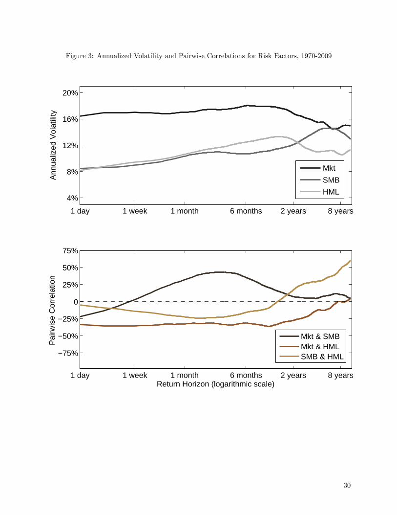
Figure 3: Annualized Volatility and Pairwise Correlations for Risk Factors, 1970-2009
1 day 1 week 1 month 6 months 2 years 8 years
−75%
−50%
−25%
0
25%
50%
75%
Return Horizon (logarithmic scale)
Pai
rwis
e C
orre
latio
n
Mkt & SMBMkt & HMLSMB & HML
1 day 1 week 1 month 6 months 2 years 8 years
4%
8%
12%
16%
20%
Ann
ualiz
ed V
olat
ility
Mkt
SMB
HML
30

evidence suggests that SMB and HML may be distinct risks over short time horizons but contain
similar fundamental risks that become evident over longer time periods.
At the same time, the SMB and HML portfolios are not nearly as attractive to a long-horizon
investor. While at a horizons of a few days these portfolios seem to have half the volatility as the
market portfolio, the volatility almost doubles when the horizon stretches to a few years. Worse
still, these portfolios that previously seemed to offer good diversification relative to the aggregate
equity market see their correlations increase significantly.
8 Implications for Short-Term Traders
While buy-and-hold investors may have poor measures of risk calculated from short-horizon
returns, active investors with a short-term focus (or even long-term investors who rebalance fre-
quently) may find short-term comovement estimates appropriately capture the portfolio risks that
matter to them. Although the underlying driver of short-horizon comovement may be fads rather
than fundamentals, it accurately reflects the one-period risks they face.
However, the relationship between correlation and time horizon reveals how one period af-
fects the next. As equation (8) emphasizes, correlation differences imply predictability. With
predictability, there is an implied trading strategy that should be attractive to tactical traders.
In this section, I will show the historical performance of a simple trading strategy based on the
comovement patterns identified. This exercise provides additional evidence that the comovement
patterns established in the empirical analysis cannot be easily explained by established risk factors.
It also frames the results in a setting familiar to other empirical studies of asset (mis)pricing where
a portfolio formation rule generates a trading strategy.
For better of for worse, this trading strategy based on comovement patterns has no anchor
suggesting the true fundamental value of any particular asset. The intuition is roughly equivalent
to that of a ”pairs trading” strategy (albeit with a much longer horizon). When the prices of two
assets with similar fundamentals diverge, the strategy puts on a long-short convergence trade. This
comes with some danger. A more savvy investor would consider the actual news and prices rather
than pursue what Stein (2009) terms an ”unanchored” trading scheme. In that sense, the trading
strategy is empirically instructive but not recommended.
31

A simple trading signal
The proposed trading signal is derived from the regression relationships for the short run return
E [rt,i|rt,j ] = E [rt,i] + ρij (1)σiσj
(rt,j − E [rt,j ]) (21)
and the long run return
E
[H−1∑τ=0
ri,t+τ |rt,j
]= E
[H−1∑τ=0
ri,t+τ
]+ ρij (H)
σiσj
(rt,j − E [rt,j ]) (22)
of rt,i conditional on rt,j . If we assume that the volatility ratio ( σiσj ) is roughly constant and the
unconditional expected return for each stock is approximately equal, then we can subtract (21)
from (23) and forecast the excess return for the future
E
[H−1∑τ=1
ri,t+τ |rt,j
]− E
[H−1∑τ=1
ri,t+τ
]= ∆ρij
σiσjrt,j . (23)
With N assets, equation (23) will yield N − 1 univariate forecasts. For simplicity, the trading
signal will weight them equally.4 The signal is then defined as
Xi,t =1
N − 1
∑j 6=i
∆ρi,jσiσjrt,j . (24)
Empirical implementation
In the empirical implementation of the trading strategy, the universe of firms will be determined
in much the same way as before, comprising the 2000 largest firms by market cap over the 40 year
sample. The set of firms will be updated annually, using data available the final business day in
December of the previous year.
To predict the future difference in long-run and short-run correlation (∆ρi,j) I use the two
main variables presented previously, where investor trading behavior is proxied by the correlation
in bid-ask bounce, νij , and fundamentals are measured as the correlation of the return on equity,
Corr[ROEi, ROEj ]. The difference between long-horizon and short-horizon correlation that de-
4An alternative would be to create the multivariate optimal forecast with GLS weights
32

termines the trading signal for forecasting in (??) can be constructed without too much fear of
overfitting from the in-sample regression results by simply taking the equal-weighted difference:
∆ρi,j ≈ Corr [ROEi, ROEj ]− νij .
These two variables are updated annually and implemented in portfolios formed each January
using information that would be available in December. The volatility ratio σiσj
is also updated
annually, and is calculated as the standard deviation of the weekly returns over the prior three
years. Shorter histories are used for any firm where three years are not available, and outliers are
winsorized at the 5th and 95th percentiles.
Signal persistence
There remains the question of how long this signal should persist. The empirical analysis
arbitrarily chose the long horizon to be H = 26 weeks but did not suggest whether the correlation
differences resolved in a matter of weeks or if the correlations continued to evolve even after the
six-month window. In the context of this trading strategy, this question is analogous to asking how
long the the signal Xt is expected to forecast excess returns.
In the framework of the simple model of fads and fundamentals presented earlier, we want to
know the decay rates δd and δf . While there is likely a high degree of variation in the characteristics
of fads and fundamentals that affect the US equity market, it is interesting to take the simplified
model and estimate the half-life of the signal.
We can do this by building a simply portfolio rule, sorting stocks into quintiles based on their
signal Xt and constructing a long-short portfolio that buys the highest quintile and sells the lowest
quintile. The event time returns to this portfolio, shown in Figure 4 will show the degree to which
the information persists.
Discuss the figure
Estimate the delta parameters
Backtest results
Given the matrix ∆β, the trading signal in (24) is obtained each week by multiplying ∆β by
the returns from the recent past. For the purposes of this backtest, I will consider the recent past to
be the returns from the past 6 weeks, omitting the most recent weeks’ returns to avoid the gaining
33
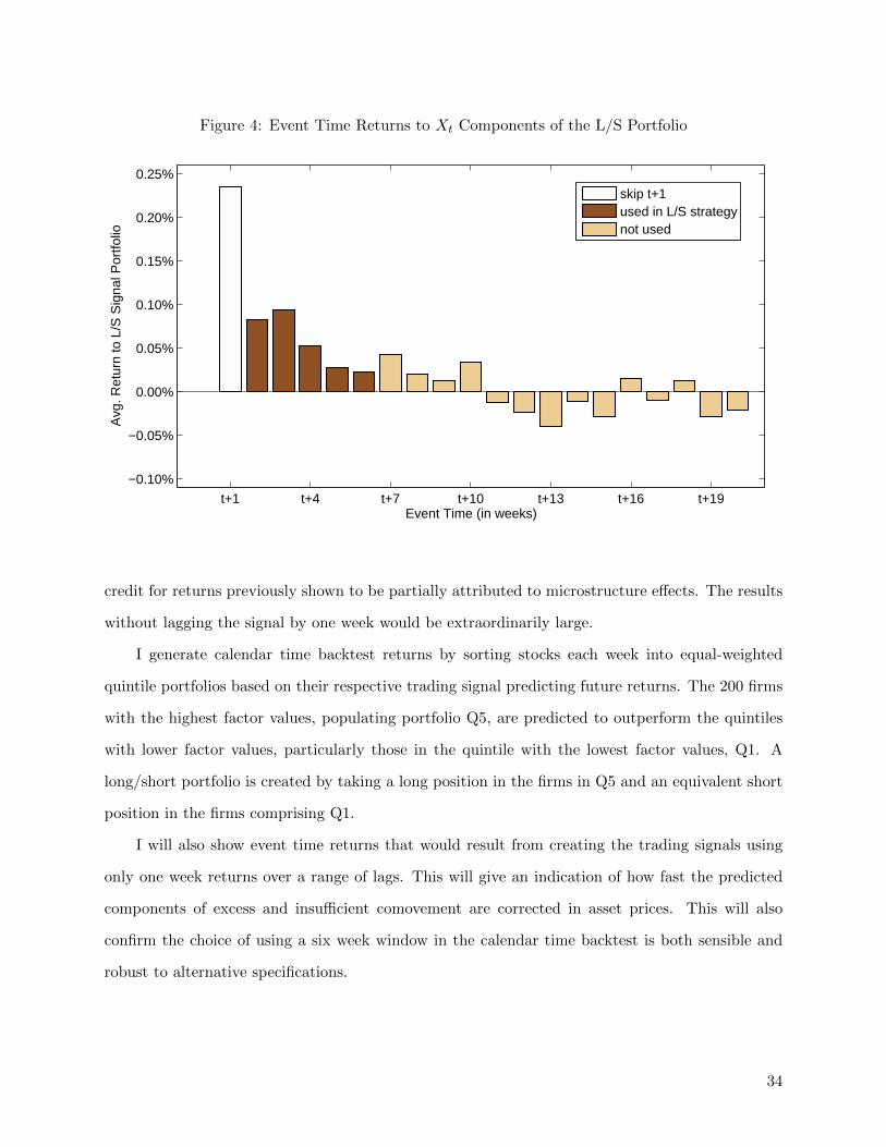
Figure 4: Event Time Returns to Xt Components of the L/S Portfolio
t+1 t+4 t+7 t+10 t+13 t+16 t+19
−0.10%
−0.05%
0.00%
0.05%
0.10%
0.15%
0.20%
0.25%
Event Time (in weeks)
Avg
. Ret
urn
to L
/S S
igna
l Por
tfolio
skip t+1used in L/S strategynot used
credit for returns previously shown to be partially attributed to microstructure effects. The results
without lagging the signal by one week would be extraordinarily large.
I generate calendar time backtest returns by sorting stocks each week into equal-weighted
quintile portfolios based on their respective trading signal predicting future returns. The 200 firms
with the highest factor values, populating portfolio Q5, are predicted to outperform the quintiles
with lower factor values, particularly those in the quintile with the lowest factor values, Q1. A
long/short portfolio is created by taking a long position in the firms in Q5 and an equivalent short
position in the firms comprising Q1.
I will also show event time returns that would result from creating the trading signals using
only one week returns over a range of lags. This will give an indication of how fast the predicted
components of excess and insufficient comovement are corrected in asset prices. This will also
confirm the choice of using a six week window in the calendar time backtest is both sensible and
robust to alternative specifications.
34

Figure 5: Annual Calendar Time Returns to L/S Portfolio
1970 1975 1980 1985 1990 1995 2000 2005 2010
−20%
−10%
0%
10%
20%
30%
40%
Ann
ual E
xces
s R
etur
n
Trading Strategy Results
The annual returns to the long/short portfolio are graphed in Figure 5. The performance of
this long/short portfolio is relatively consistent over time and does not show a tendency to decrease
over time. This is true even in the most recent decade when you might expect that trading by
hedge funds, especially so-called statistical arbitrage funds, might employ similar strategies and
erode the returns available to a comovement based strategy.
The strong recent performance is also surprising given the fact that, on average, short-horizon
and long-horizon comovement have converged. This result suggests that the dispersion of comove-
ment differences across firms remains large and predictable even while the average is near zero.
Looking again at the annual returns to the strategy, the most profitable of the 40 years considered
was 2008, with a return of 28.8%. Over the 40-year sample, the long/short portfolio generates an
average annual excess return of 5.3% with a corresponding Sharpe Ratio of 0.65.
The weekly event time returns, shown in Figure 4, provide additional insight on the nature of
the portfolio returns. These event time returns only interact one week of past returns (dated rt)
35
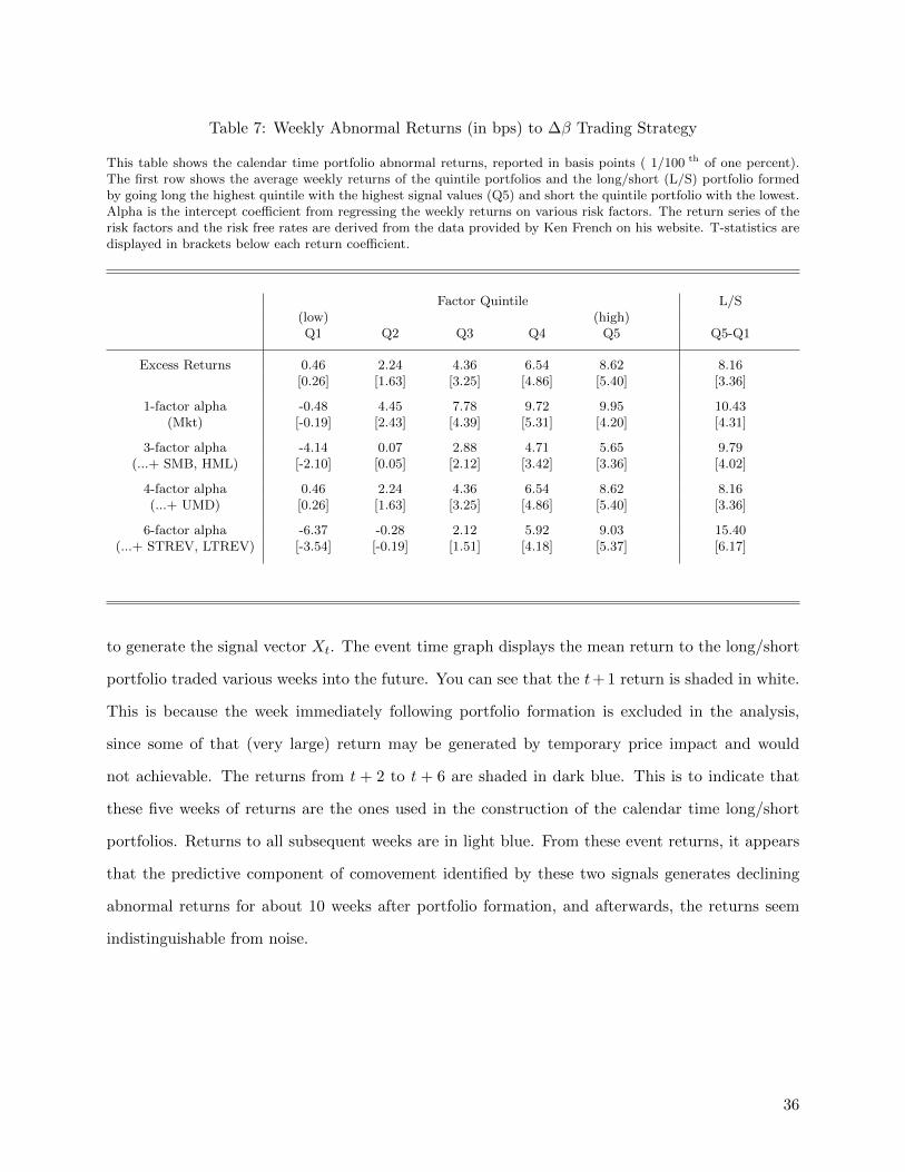
Table 7: Weekly Abnormal Returns (in bps) to ∆β Trading Strategy
This table shows the calendar time portfolio abnormal returns, reported in basis points ( 1/100 th of one percent).The first row shows the average weekly returns of the quintile portfolios and the long/short (L/S) portfolio formedby going long the highest quintile with the highest signal values (Q5) and short the quintile portfolio with the lowest.Alpha is the intercept coefficient from regressing the weekly returns on various risk factors. The return series of therisk factors and the risk free rates are derived from the data provided by Ken French on his website. T-statistics aredisplayed in brackets below each return coefficient.
Factor Quintile L/S(low) (high)Q1 Q2 Q3 Q4 Q5 Q5-Q1
Excess Returns 0.46 2.24 4.36 6.54 8.62 8.16[0.26] [1.63] [3.25] [4.86] [5.40] [3.36]
1-factor alpha -0.48 4.45 7.78 9.72 9.95 10.43(Mkt) [-0.19] [2.43] [4.39] [5.31] [4.20] [4.31]
3-factor alpha -4.14 0.07 2.88 4.71 5.65 9.79(...+ SMB, HML) [-2.10] [0.05] [2.12] [3.42] [3.36] [4.02]
4-factor alpha 0.46 2.24 4.36 6.54 8.62 8.16(...+ UMD) [0.26] [1.63] [3.25] [4.86] [5.40] [3.36]
6-factor alpha -6.37 -0.28 2.12 5.92 9.03 15.40(...+ STREV, LTREV) [-3.54] [-0.19] [1.51] [4.18] [5.37] [6.17]
to generate the signal vector Xt. The event time graph displays the mean return to the long/short
portfolio traded various weeks into the future. You can see that the t+ 1 return is shaded in white.
This is because the week immediately following portfolio formation is excluded in the analysis,
since some of that (very large) return may be generated by temporary price impact and would
not achievable. The returns from t + 2 to t + 6 are shaded in dark blue. This is to indicate that
these five weeks of returns are the ones used in the construction of the calendar time long/short
portfolios. Returns to all subsequent weeks are in light blue. From these event returns, it appears
that the predictive component of comovement identified by these two signals generates declining
abnormal returns for about 10 weeks after portfolio formation, and afterwards, the returns seem
indistinguishable from noise.
36
Adjusting the calendar time returns for risk exposures
The average weekly excess returns alphas for the calendar time analysis of the five quintile
portfolios and the long/short portfolio are presented in Table 6. As would be desired, there is a
consistent pattern of returns increasing by quintile. In the unadjusted excess returns, the lowest
quintile portfolio earns only 0.46 basis points per week versus the 8.6 basis point average return
of the highest quintile, which corresponds to an annual return of 0.24%. The 8 basis point weekly
return of the long/short portfolio has an associated t-statistic of 3.36, indicating we can confidently
reject the notion that the true excess return of the strategy is zero.
Table 6 also reports the alphas for each portfolio after controlling for risk factors known to
generate positive returns. These alphas are the intercept in the regression of the weekly returns
of risk factors on the returns to the quintile and long/short portfolios. Four factor models are
considered, and the Tuesday-to-Tuesday weekly returns for each of the component risk factors are
derived from the daily research returns available on Ken French’s website5. The first two models
include a 1-factor model that controls for exposure to the value-weighted market index, and the
3-factor alpha, that additionally includes the SMB and HML factors popularized by Fama and
French (1992).
In addition to these standard benchmarks, we might wonder if the returns to portfolios based on
comovement are related to momentum and reversal patterns found to empirically generate positive
returns in the cross-section of US equities. To answer this, we can introduce two additional models,
a 4-factor model including Carhart’s (1997) momentum factor, and finally, a 6-factor model which
additionally includes short-term and long-term reversal patterns. These reversal returns are defined
by French to be the lagged one month return and the past 5-year return excluding the most recent
year. Interestingly, this comovement trading strategy tends to trade in the opposite direction of
these reversal factors, making the alphas look even more compelling. The long/short portfolio,
which averages 8.2 basis points of excess returns weekly, reports a 6-factor alpha of 15.4 basis
points. Translated to an annual time frequency, these risk adjusted returns would yield an average
return of 8.4% and a Sharpe Ratio of 1.03.
5http://mba.tuck.dartmouth.edu/pages/faculty/ken.french/data library.html
37
9 Conclusion
Asset price comovement changes with time horizon. The evidence is consistent with a model
where fads and information delays cause prices to temporarily deviate from fundamentals. In
particular, there is compelling evidence that investor trading behavior and salient security charac-
teristics are more important factors in determining the correlation of US equity returns over short
horizons while measures of long-run fundamentals play a greater role in return correlations over
longer horizons.
I propose the difference between short-horizon and long-horizon comovement is a natural metric
for studying excess comovement. Measures of common trading behavior and shared economic
fundamentals show significant power in explaining cross-sectional differences in excess comovement
across pairs of stocks. They can also form a successful trading strategy. A portfolio based on
predictable differences in stock correlations generates consistent excess returns not explained by
risk exposures.
The main implication for investors with a buy and hold strategy is that they may be underesti-
mating (or overestimating) the risk concentration of their portfolio if they extrapolate comovement
and volatility from short-horizon returns. This also suggests a degree of caution to financial econo-
metricians who propose the use of intra-day data to estimate the covariance of security returns. It
would seem that using ever shorter return horizons to estimate second moments will likely capture a
greater degree of comovement driven by trading behavior rather than the fundamentals that matter
over longer horizons.
Although the empirical evidence presented here focuses on US equities, the principle should
apply just as much in other asset classes as well as in the broader asset allocation decision. In
fact, there is reason to believe differences in comovement may be even larger across asset classes, as
market segmentation may be more pronounced. The relationship between correlation and return
horizon may identify risks and opportunities that can arise as short-run comovement deviates from
long-run fundamentals.
38
References
Anton, M. and C. Polk (2010). Connected Stocks. Working Paper, London School of Eco-nomics (May).
Barberis, N. and A. Shleifer (2003, May). Style investing. Journal of Financial Economics 68 (2),161–199.
Barberis, N., A. Shleifer, and J. Wurgler (2005, February). Comovement. Journal of FinancialEconomics 75 (2), 283–317.
Boyer, B. H. (2011, February). Style-Related Comovement: Fundamentals or Labels? The Journalof Finance 66 (1), 307–332.
Brealey, R. A., I. A. Cooper, and E. Kaplanis (2009, December). Excess Comovement in Interna-tional Equity Markets: Evidence from Cross-border Mergers. Review of Financial Studies 23 (4),1718–1740.
Campbell, J. Y., S. Grossman, and J. Wang (1993). Trading Volume and Serial Correlation inStock Returns. Quarterly Journal of Economics 108 (4), 905–939.
Campbell, J. Y., M. Lettau, G. M. Burton, and Y. Xu (2001). Have Individual Stocks BecomeMore Volatile? An Empirical Exploration of Idiosyncratic Risk. The Journal of Finance 56 (1),1–43.
Cochrane, J. H. (1991, June). Volatility tests and efficient markets A review essay. Journal ofMonetary Economics 27 (3), 463–485.
Cohen, R. B., C. Polk, and T. Vuolteenaho (2009). The Price Is (Almost) Right. Journal ofFinance 64 (6), 2739–2782.
Dabora, E. M. and K. A. Froot (1999). How are stock prices affected by the location of trade?Journal of Financial Economics (2), 189–216.
Fama, E. F. and K. R. French (1988). Permanent and Temporary Components of Stock Prices.The Journal of Political Economy 96 (2), 246–273.
Greenwood, R. (2008, March). Excess Comovement of Stock Returns: Evidence from Cross-Sectional Variation in Nikkei 225 Weights. Review of Financial Studies 21 (3), 1153–1186.
Greenwood, R. and D. Thesmar (2011, July). Stock Price Fragility. Journal of Financial Eco-nomics 102 (3), 490–471.
Kumar, A. and C. M. Lee (2006, October). Retail Investor Sentiment and Return Comovements.The Journal of Finance 61 (5), 2451–2486.
Lo, A. W. and A. C. MacKinlay (1990, April). When are contrarian profits due to stock marketoverreaction? Review of Financial Studies 3 (2), 175–205.
Newey, W. K. and K. D. West (1987). A Simple, Positive Semi-Definite, Heteroskedasticity andAutocorrelation Consistent Covariance Matrix. Econometrica 55 (3), 703–708.
Pindyck, R. S. and J. J. Rotemberg (1993). The Comovement of Stock Prices. Quarterly Journalof Economics 108 (4), 1073–1104.
39

Roll, R. (1984). A Simple Implicit Measure of the Effective Bid-Ask Spread in an Efficient Market.Journal of Finance 39 (4), 1127–1139.
Shiller, R. J. (1981). Do Stock Prices Move Too Much to be Justified by Subsequent Changes inDividends. American Economic Review (3), 421–436.
Stein, J. C. (2009, August). Presidential Address: Sophisticated Investors and Market Efficiency.The Journal of Finance 64 (4), 1517–1548.
Veldkamp, L. L. (2006, July). Information Markets and the Comovement of Asset Prices. Reviewof Economic Studies 73 (3), 823–845.
40